Kondo Screening Cloud Scaling: Impurity Entanglement and Magnetization
Abstract
The screening of an impurity spin in the Kondo model occurs over a characteristic length scale , that defines the size of the Kondo screening cloud or “mist”. The presence of such a length scale in experimental and numerical results is rather subtle. A consistent way to show the presence of the screening cloud is to demonstrate scaling in the spatial correlations depending on , in terms of the single variable rather than depending on and separately. Here we study the paradigmatic one channel Kondo model using a spin chain representation, with an impurity spin at one end of the chain coupled with a strength . Using Fermi liquid theory combined with numerical results, we obtain new high precision estimates of the non-universal terms in the entanglement entropy which leads to a verification of the expected non-integer ground-state degeneracy, . This then allows us to study the impurity contribution to the entanglement in detail. If the impurity coupling is varied, a precise determination of can then be obtained. The length scale, , is then shown to characterize the scaling of both the uniform and alternating part of a measure of the magnetization of part of an odd length chain with.
1 Introduction
The Kondo effect [1, 2, 3] continues to yield surprising insights. In its simplest form, the Kondo effect describes the coupling of a single impurity spin to a bath of non-interacting conduction electrons. In the absence of any coupling, the electrons are undisturbed by the impurity, while at very strong coupling, a single electron is trapped by the impurity, forming a singlet at the impurity site. Intuitively, one might then expect that at intermediate coupling the low energy physics is again described by the formation of a singlet state between the conduction electrons and the impurity spin, often described as a screening cloud [4]. Only a single electron is needed to form this singlet, but in this case the screening singlet could be macroscopic in size. The natural length scale associated with this phenomenon is with the velocity of the low energy excitations and the Kondo temperature, and for , could extend into the regime for typical values of . It is important to realize that this screening cloud [4] which forms the singlet with the impurity only involves a single electron even though it is of course a many-body state, and it is perhaps better described as a “mist”. The presence of the screening cloud is therefore a particular subtle feature of the Kondo effect, since it involves spatial correlations around the impurity out to large distances involving a single electron. It is natural to ask what it actually means to have a screening cloud. The best definition is that physical quantities should obey a scaling form [5] in instead of depending on and independently, this then implies variations over at least a distance of . In fact, it is by demonstrating such scaling in experimental data that the presence of the Kondo screening cloud has recently been detected in experiments on quantum dots coupled to a quasi-one-dimensional channel [6].
A focus of particular current interest has been the entanglement between the impurity and the electrons [7]. In the strong coupling limit where a single electron is trapped at the impurity site into a singlet state, other electrons are not allowed onto the site since it would destroy the singlet, and we do not expect the impurity to significantly alter the entanglement. However, for intermediate couplings, the impurity contribution to the entanglement can be shown to again follow a scaling form [7, 8]. At finite temperatures, the negativity is a convenient measure of the impurity entanglement [9] and the thermal decay of the negativity has been shown to obey a characteristic power-law form [10, 11]. More generally, the entanglement across conformal and topological defects has been investigated [12, 13, 14] and the Kondo effect in spin liquids has been studied [15, 16, 17, 18, 19], but the corresponding entanglement has so far only received limited attention. A difficulty is here that non-universal terms appear in the entanglement entropy that are often not known with sufficient precision. Furthermore, the impurity contribution to the entanglement is defined by subtracting the bulk contribution, which is often a challenging procedure. Here we revisit the one channel Kondo model and study the impurity entanglement in detail. With open boundary conditions a contribution arising from the non-integer ground-state degeneracy, [20], can only be precisely determined if the impurity entanglement from open boundaries are taken into account. We then turn to the magnetization, demonstrating similar scaling with .
We shall here take the coupling between the impurity spin and the conduction electrons to be a delta-function. The spherical symmetry of the coupling implies that the problem can be reduced to a one-dimensional model after an expansion in harmonics since only the s-wave harmonic interacts with the impurity. If one linearizes the dispersion relation around the Fermi momentum, , one can then write a one-dimensional effective Hamiltonian in terms of left and right moving Fermi fields that are functions of and , respectively, obeying the anti-commutation relation :
| (1.1) |
Here, is the radial coordinate and the impurity is now situated at with the electrons confined to a semi-infinite line and
| (1.2) |
is the electron spin density at and the boundary condition is imposed at the origin. Here, is the coupling between the impurity spin and the electron spin density. (See, for example, [21] for more details.) Since this model explicitly refer to electronic degrees of freedom, we refer to this model as the free electron Kondo model (FEKM).
A model closely to the one-dimensional FEKM consists of an open gap-less spin- Heisenberg chain, defined on a semi-infinite line, with one coupling at the end of the chain weaker than the others, described by the following Hamiltonian.
| (1.3) |
It turns out that a low energy field theory description of this spin chain model is essentially the same as Eq. (1.1), and one may therefore think of Eq. (1.3) as a spin chain Kondo model (SCKM) [7, 8, 22] equivalent to the one-channel Kondo model. In fact, it turns out that in the limit , a very simple linear relation exists between in Eq. (1.1) and in Eq. (1.3), [22]. For =1 this model is the well-known - spin model that with =0 is simply the antiferromagnetic Heisenberg chain. However, we shall only be interested in a very specific value of , corresponding to a critical point [23]:
| (1.4) |
At this value of a bulk marginally irrelevant coupling becomes exactly zero [24], leading to the disappearances of logarithmic corrections, a significant advantage for numerical work. For the SCKM develops a gap and orders in a dimer state, and the correspondence to the FEKM no longer holds. Another advantage of the SCKM is the significant reduction in the on-site degrees of freedom, which means that higher precision results can be obtained with fewer resources.
As a measure of the entanglement, we mainly focus on the von Neumann entanglement entropy. For a subsystem of linear length the entanglement entropy is defined in terms of the corresponding reduced density matrix, ,
| (1.5) |
where is obtained from the ground-state wave-function. To study the entanglement entropy and the magnetization in the SCKM, we use density matrix renormalization group techniques [25, 26, 27, 28, 29, 30, 31] (DMRG) on finite chains of length up to , typically with .
We begin with an analysis of quantum impurity entanglement in the SCKM, building on previous studies [5, 7, 8, 22, 32]. Here we significantly extend and refine many of the results. All the results in this section are obtained using the SCKM, Eq. (1.3) at ==. As mentioned above, at this value of corrections arising from the bulk marginal operator are absent, significantly improving the precision of the results. In the subsequent sections, we then turn to a discussion of our results for the magnetization.
2 Entanglement in the Periodic Chain,
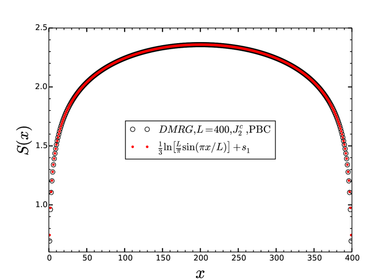
First, we focus on the purely periodic chain with since this will allow us to determine non-universal constants that are crucial for our subsequent analysis. From analytical results [33, 34] it is known that for a finite periodic system of sites, the entanglement entropy of a sub-system of size is:
| (2.1) |
where is the central charge and is a non-universal constant. For the models we consider, we have . Our DMRG results with for are shown in Fig. 1 for a periodic chain with . With periodic boundary conditions (PBC) there is no boundary and is smoothly varying as the size of the sub-system changes. The DMRG results can be fitted extremely well to the expected form, Eq. (2.1), from which we obtain at :
| (2.2) |
Note that, is non-universal and for instance depends on . Hence, at the isotropic Heisenberg point with , we find a slightly smaller value of . One may also note that the for the non-interacting chain has been determined to be [35]. The variation in between the different models is surprisingly small.
3 Fermi Liquid Theory
Consider now the uniform =1/2 SCKM chain with open boundary conditions (OBC) of interest here. The chain has length and we consider a region at one end of the open chain of length . As shown in [35], one effect of the open boundary conditions is to induce an alternating term , in the von Neumann entanglement entropy, . The latter is therefore best view as composed of a uniform and alternating term
| (3.1) |
with both and smoothly varying functions. If the bulk of the system is uniform, the alternating term decays to zero with . However, recent work has shown that if the sub-system starts at the boundary and ends at an impurity, then the alternating term does not necessarily decay to zero [36]. The bulk contribution to the uniform part of the von Neumann entanglement entropy, , is given by [33, 34, 37, 38]:
| (3.2) |
In contrast to the constant is a universal term arising from a non-integer ground-state degeneracy, [20]. However, this is not the only contribution to since the open ends of the chain gives rise to a boundary term, [7, 8], so that
| (3.3) |
It is possible to describe the leading contributions to using conformal field theory (CFT) methods based on Nozières local Fermi liquid theory (FLT) [39, 21, 40, 41]. The leading contributions, due to the two open ends, are caused by the leading irrelevant operator where is the energy density, in Abelian bosonization, and is a coupling constant of order a lattice spacing. The first order correction due to , the boundary interaction at the left end of the system, was calculated in Ref. [7]:
| (3.4) |
This result is valid in the FLT regime:
| (3.5) |
There is another correction due to , the boundary operator at the right end of the system. This can be obtained by substituting , thereby obtaining:
| (3.6) |
where we have used the standard relation . Since the analysis in Refs. [7, 8] involved a subtractive procedure, approximately eliminating , this term was not included. Following the convention adopted in [7, 22] we identify with , where can be identified with the size of the Kondo screening cloud. With this normalization, the zero-temperature impurity susceptibility is . The total correction arising from both ends of the open chain is then:
| (3.7) |
This is symmetric under and is functionally similar to up to an overall multiplicative constant and in Ref. [35] the leading correction term to Eq. (3.2) arising from the open boundary was therefore assumed to be of the form instead of the correct form, Eq. (3.7).
If we consider a slightly modified coupling, , of the spin at the left end of the chain, the boundary operator will still appear but with a different coupling constant which we can write as . If we denote the coupling on the right side as , we obtain:
| (3.8) |
with from Eq. (3.2). Note that in the limit we have [7]:
| (3.9) |
with a similar expression for . Hence, both and remain finite in the thermodynamic limit at fixed . On the other hand, they can be neglected if is kept fixed as .
4 Impurity Entanglement in the Open Chain,
We begin by considering the uniform open chain, with =1, performing DMRG calculations on a system with . We first extract the uniform part of the entanglement entropy, . This is done using a 9-point stencil as described in A. We then fit the results for directly to Eq. (3.8). With only and as the two free parameters, we obtain an excellent fit, see solid red line in Fig. (2). We explicitly determine:
| (4.1) |
With the previously determined value for we can now determine finding:
| (4.2) |
in excellent agreement with the theoretical result, [42, 38]. It is important to note that the precision of the numerical result crucially relies on the detailed understanding of the correction term Eq. (3.7). A similar analysis at a is complicated by additional corrections arising from the bulk marginal operator, rendering a high precision determination of very challenging.
In order to focus solely on the contribution arising from the two ends of the open chain we define:
| (4.3) |
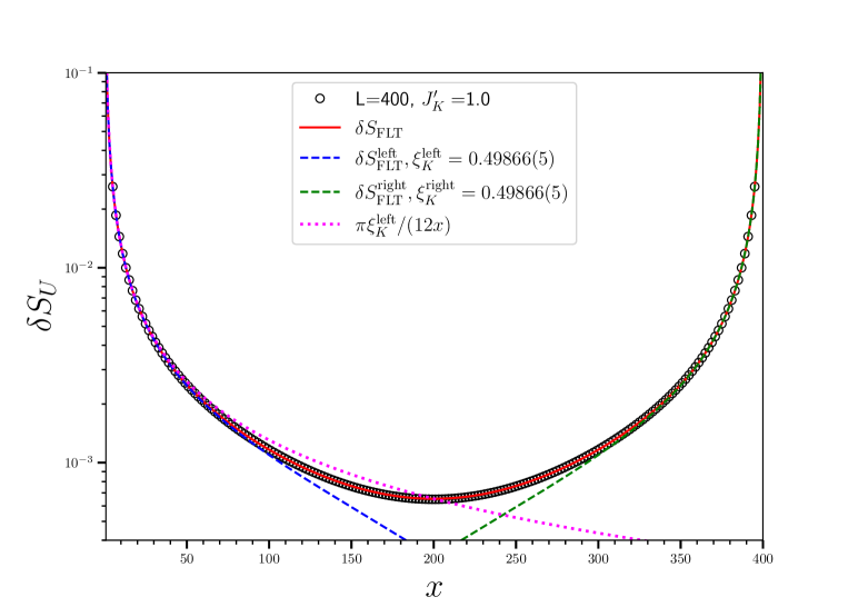
with given in Eq. (3.2). Our results for for the uniform open chain with are shown in Fig. 2. An excellent agreement between the numerical results (black circles) and the fit to Eq. (3.7) (solid red line) is evident. Since the analytical expression is not valid for we fit only data for . With the above validation of the term and the value of from the results with PBC, Eq. (2.2), we fix these parameters and perform a one parameter fit in determining:
| (4.4) |
We note, that a similar analysis at yields a significantly larger estimate of . For completeness, the separate contributions from , Eq. (3.4) and , Eq. (3.6) are shown as the dashed blue and green lines, respectively, in Fig. 2. For comparison, we also show the thermodynamic limit FLT result, Eq. (3.9) (dotted magenta line) which agrees very convincingly with the numerical results at small although the finite corrections, accounted for in Eq. (3.7), are visible for .
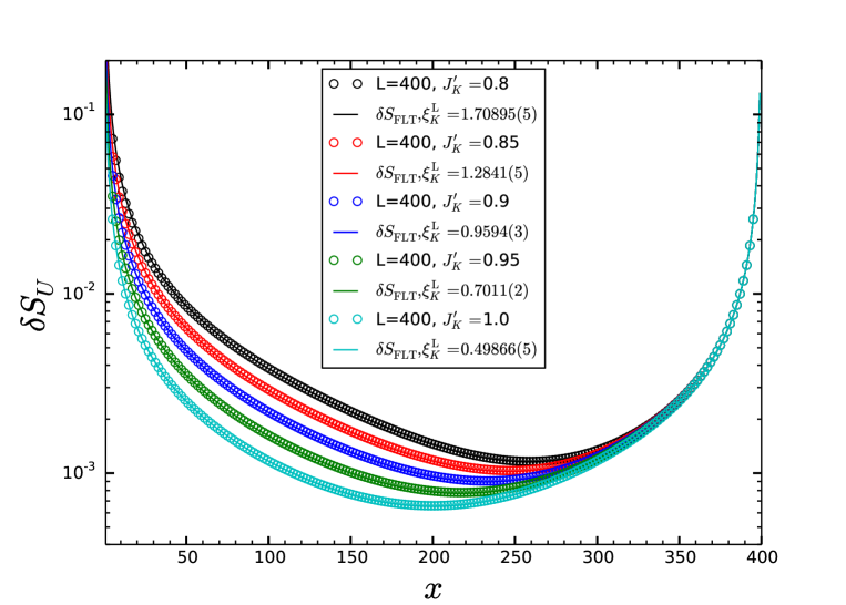
It is now possible to obtain very precise estimates for as a function of by performing numerical calculations with a range of at the left end of the chain, (see Eq. (1.3), thereby varying . With the known values of as well as , Eq. (4.1), we then perform a one parameter fit of to the analytical FLT form , Eq. (3.8). Our results are shown in Fig. 3 for with the solid lines representing the fitted form. An excellent agreement between the numerical data and analytical expression can be seen. Again, we restrict the fits to to be sure we are in the FLT regime, Eq. (3.5). We typically use and since we also must require that we stop the calculations at where reaches the value of 11.824(4). It would of course be relatively straight forward to repeat the calculations with , however, since it quickly becomes unfeasible to extract for smaller by fitting numerical results to Eq. (3.8).
| 1.00 | 0.49866(5) | 0.90 | 0.9594(3) | 0.80 | 1.7293(5) | 0.70 | 3.066(2) | 0.60 | 5.708(2) |
| 0.99 | 0.5361(1) | 0.89 | 1.0308(3) | 0.79 | 1.8296(7) | 0.69 | 3.253(2) | 0.59 | 6.112(2) |
| 0.98 | 0.5749(1) | 0.88 | 1.0936(4) | 0.78 | 1.9396(8) | 0.68 | 3.456(2) | 0.58 | 6.540(2) |
| 0.97 | 0.6152(1) | 0.87 | 1.1595(4) | 0.77 | 2.0524(8) | 0.67 | 3.676(3) | 0.57 | 7.006(2) |
| 0.96 | 0.6572(2) | 0.86 | 1.2289(5) | 0.76 | 2.1720(9) | 0.66 | 3.906(1) | 0.56 | 7.524(2) |
| 0.95 | 0.7011(2) | 0.85 | 1.3018(5) | 0.75 | 2.2989(9) | 0.65 | 4.152(2) | 0.55 | 8.082(2) |
| 0.94 | 0.7513(2) | 0.84 | 1.3785(5) | 0.74 | 2.4337(9) | 0.64 | 4.418(2) | 0.54 | 8.693(2) |
| 0.93 | 0.7999(2) | 0.83 | 1.4593(6) | 0.73 | 2.5770(9) | 0.63 | 4.704(2) | 0.53 | 9.365(3) |
| 0.92 | 0.8507(3) | 0.82 | 1.5445(6) | 0.72 | 2.730(1) | 0.62 | 5.013(2) | 0.52 | 10.104(4) |
| 0.91 | 0.9038(3) | 0.81 | 1.6344(7) | 0.71 | 2.892(1) | 0.61 | 5.346(2) | 0.51 | 10.920(5) |
It is often very useful to have high precision numerical data for available, and we have collected some of our results for in Table 1. Again, we stress that these results are obtained at and similar calculations at and in particular at yield larger values for .
5 as a function of
Through perturbative calculations as detailed in [22], can be related to the coupling in Eq. (1.1) as follows: Furthermore, through a careful determination of the spin velocity and by studying end to end correlation functions, it was shown [22] that in the limit , at , the following relation between and holds
| (5.1) |
In terms of we therefore have
| (5.2) |
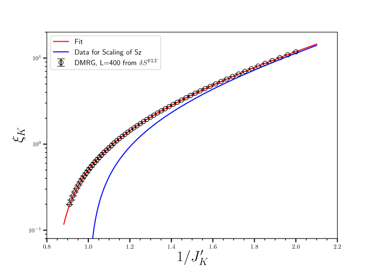
Here, the term represents a power series in . Note that, for , the behavior is slightly different and instead one has [22]. It is straightforward to verify that our results obey this relation very precisely. As shown in Fig. 4 we can fit the numerical data from Table 1 to Eq. (5.2) obtaining
| (5.3) |
In this fit the previously estimated constant is held fixed and as is clearly evident in Fig. 4 at large the exponential divergence is clearly in agreement with this independently determined constant. The addition of the correction terms allows the form Eq. (5.2) to fit the data even for relatively large even exceeding 1. This indicates that a critical value exists at which the correction vanishes. This coupling can be estimated to be:
| (5.4) |
6 Scaling of for Odd Length Chains
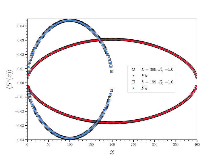
We now turn to an analysis of scaling of the magnetization occurring in odd length systems and we focus exclusively on the ground-state with =1/2. Since the system is antiferromagnetic and the length is odd, will have both a uniform and alternating part. We write:
| (6.1) |
Our goal here is to develop a scaling form for the uniform and alternating part of the magnetization as the coupling to the impurity spin, , is varied. In the case of the uniform chain with () at , it was shown [43] that for the alternating part, , of in the subspace:
| (6.2) |
At small the alternating part then increases in a characteristic manner. There is also a uniform part, , which in the middle of the chain is well approximated by the constant . We note that for the calculations we consider here in the subspace we must have . Our fits to this form are shown in Fig. 5 yielding excellent agreement with Eq. (6.2) allowing us to determine . Here, the calculations are performed at . At smaller values of corrections to the form Eq. (6.2) occur [44].
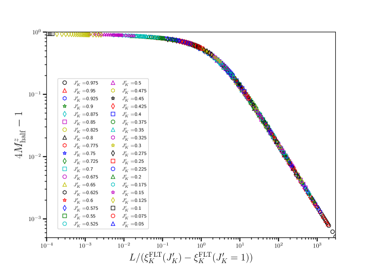
At the isotropic point, , the on-site magnetization is also symmetric around the site which means that we can define the half-magnetization:
| (6.3) |
Since and since encompasses half of this magnetization when it follows that at . Note that the impurity spin resides on site . In the other limit of we instead find since the effectively decoupled impurity spin at will carry all the magnetization so that . However, for intermediate, we expect to only depend on the single variable and follow the scaling form:
| (6.4) |
as is varied between and . We want to demonstrate this scaling using the previously determined , however, for the quantity the strong coupling fixed point where corresponds whereas for occurs for . In order to correct for this difference, we therefore need to scale the data for using instead of just . In Fig. 6 we show numerical results for displaying excellent scaling with with obtained from . (See Table 1.)
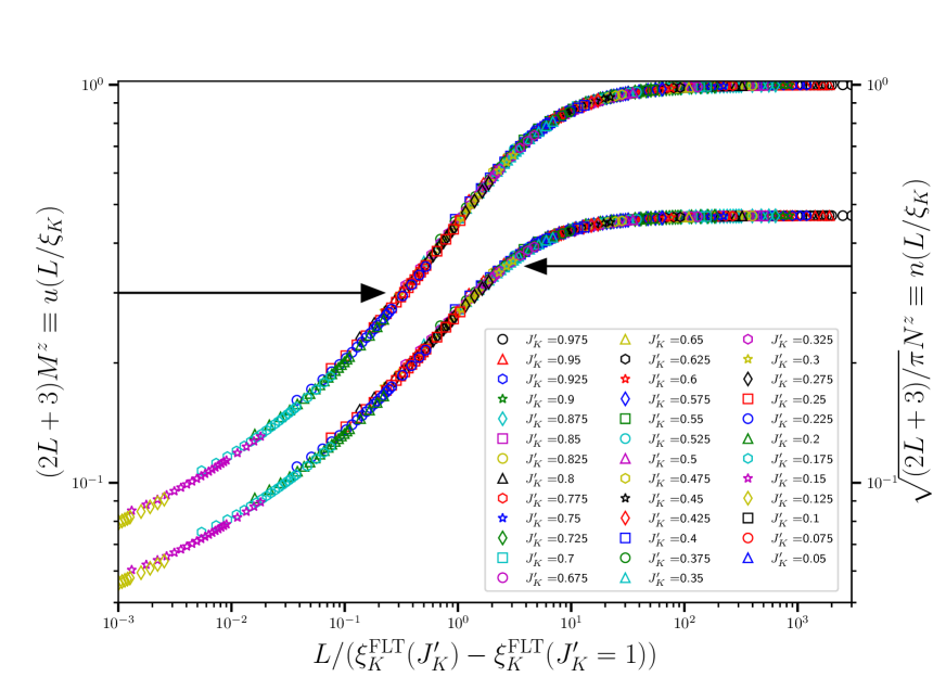
Building on the relations, Eq. (6.1) and (6.2), we can also construct scaling forms for and . Again we focus on the middle of the chain and extract the uniform and alternating part of . We then expect to find:
| (6.5) |
as well as
| (6.6) |
with and scaling functions. We note that for the impurity spin itself and for the site coupled to it, weak scaling violations should be observed [22] due to the presence of an anomalous dimension for the corresponding operator [45]. For both the prefactors of for and for , it is only the overall dependence that is known, with the precise additive constant determined numerically. As was the case for , the strong coupling fixed point where again corresponds to and we therefore again use instead of just . Our results are shown in Fig. 7 where data for both the scaled and are shown together. An excellent scaling of the data when plotted versus is evident. However, in the limit deviations are clearly visible as one would expect. Similar deviations from scaling for are visible in Fig. (6) but are obscured by the fact that approaches 1 in the limit.
7 Discussion
Using a spin chain representation of the one-channel Kondo model we have shown that scaling with the Kondo length scale is obeyed to a high degree of precision and that reliable estimates of can be obtained. For the open chain it is clear that apart from the usual term proportional to the central charge, the entanglement entropy contains two other terms, an alternating term but also an impurity term arising from the boundary. We have also demonstrated that the same length scale, , from our analysis of the entanglement entropy can be used to scale the magnetization present in a sub-system of the chain if a proper normalization is taken into account. The analysis of the magnetization is in some sense simpler since it directly yields the impurity contribution without involving a subtractive procedure.
Appendix A Extracting the Uniform and Alternating Parts
For the analysis of the data, it is necessary to extract the uniform and alternating part of a function defined on discrete points . Focusing on a point , we make the following assumption [8]:
| (1.1) |
In the vicinity of the point we can then develop a 7-point stencil by assuming that and are well approximated by slowly varying polynomials: and , for , arriving at the equations:
As can easily be verified, the solutions for are then:
| (1.3) | |||||
| (1.4) |
In Ref. [8] a slight variation on these solutions were used. The above equations have the advantage that they are explicitly invariant under , and as one would expect. Note that, as we move along the chain, the sign of will vary. An equivalent 9-point stencil can be derived, yielding:
| (1.5) | |||||
| (1.6) |
References
- [1] Jun Kondo. Resistance minimum in dilute magnetic alloys. Progress of Theoretical Physics, 32:37–49, 1964.
- [2] A. C. Hewson. The Kondo Problem to Heavy Fermions. Cambridge University Press, 2000.
- [3] N. Andrei, K. Furuya, and J. H. Lowenstein. Solution of the kondo problem. Rev. Mod. Phys., 55(2):331–402, Apr 1983.
- [4] Ian Affleck. The kondo screening cloud: what it is and how to observe it. In Amnon Aharony and Ora Entin-wohlman, editors, Perspectives Of Mesoscopic Physics: Dedicated To Yoseph Imry’s 70th Birthday, chapter 1, pages 1–45. World Scientific, 2010.
- [5] Erik S. Sørensen and Ian Affleck. Scaling theory of the kondo screening cloud. Phys. Rev. B, 53:9153–9167, Apr 1996.
- [6] Ivan V. Borzenets, Jeongmin Shim, Jason C. H. Chen, Arne Ludwig, Andreas D. Wieck, Seigo Tarucha, H.-S. Sim, and Michihisa Yamamoto. Observation of the kondo screening cloud. Nature, 579:210–213, 2020.
- [7] Erik S. Sørensen, Ming-Shyang Chang, Nicolas Laflorencie, and Ian Affleck. Impurity entanglement entropy and the kondo screening cloud. Journal of Statistical Mechanics: Theory and Experiment, 2007(01):L01001, 2007.
- [8] Erik S. Sørensen, Ming-Shyang Chang, Nicolas Laflorencie, and Ian Affleck. Quantum impurity entanglement. Journal of Statistical Mechanics: Theory and Experiment, 2007(08):P08003, 2007.
- [9] Abolfazl Bayat, Pasquale Sodano, and Sougato Bose. Negativity as the entanglement measure to probe the kondo regime in the spin-chain kondo model. Phys. Rev. B, 81:064429, Feb 2010.
- [10] S.-S. B. Lee, Jinhong Park, and H.-S. Sim. Macroscopic quantum entanglement of a kondo cloud at finite temperature. Phys. Rev. Lett., 114:057203, Feb 2015.
- [11] Donghoon Kim, Jeongmin Shim, and H.-S. Sim. Universal thermal entanglement of multichannel kondo effects. Phys. Rev. Lett., 127:226801, Nov 2021.
- [12] Ananda Roy and Hubert Saleur. Entanglement entropy in the ising model with topological defects. Phys. Rev. Lett., 128:090603, Mar 2022.
- [13] David Rogerson, Frank Pollmann, and Ananda Roy. Entanglement entropy and negativity in the ising model with defects. Journal of High Energy Physics, 2022:165, 2022.
- [14] Luca Capizzi and Viktor Eisler. Zero-mode entanglement across a conformal defect. Journal of Statistical Mechanics: Theory and Experiment, 2023(5):053109, may 2023.
- [15] Alexei Kolezhuk, Subir Sachdev, Rudro R. Biswas, and Peiqiu Chen. Theory of quantum impurities in spin liquids. Phys. Rev. B, 74:165114, Oct 2006.
- [16] Kusum Dhochak, R. Shankar, and V. Tripathi. Magnetic impurities in the honeycomb kitaev model. Phys. Rev. Lett., 105:117201, Sep 2010.
- [17] S. D. Das, K. Dhochak, and V. Tripathi. Kondo route to spin inhomogeneities in the honeycomb kitaev model. Phys. Rev. B, 94:024411, Jul 2016.
- [18] Wen-Yu He and Patrick A. Lee. Magnetic impurity as a local probe of the (1) quantum spin liquid with spinon fermi surface. Phys. Rev. B, 105:195156, May 2022.
- [19] Shuangyuan Lu and Yuan-Ming Lu. Detecting symmetry fractionalization in gapped quantum spin liquids by magnetic impurities, arXiv:2209.09853, 2022.
- [20] Ian Affleck and Andreas W. W. Ludwig. Universal noninteger “ground-state degeneracy” in critical quantum systems. Phys. Rev. Lett., 67:161–164, Jul 1991.
- [21] I. Affleck. A current algebra approach to the kondo effect. Nucl. Phys. B, 336:517, 1990.
- [22] Nicolas Laflorencie, Erik S. Sørensen, and Ian Affleck. The kondo effect in spin chains. Journal of Statistical Mechanics: Theory and Experiment, 2008(02):P02007, 2008.
- [23] Sebastian Eggert. Numerical evidence for multiplicative logarithmic corrections from marginal operators. Phys. Rev. B, 54:R9612–R9615, Oct 1996.
- [24] Sebastian Eggert and Ian Affleck. Magnetic impurities in half-integer-spin Heisenberg antiferromagnetic chains. Phys. Rev. B, 46:10866–10883, Nov 1992.
- [25] S. R. White and R. M. Noack. Real-space quantum renormalization groups. Phys. Rev. Lett., 68:3487–3490, Jun 1992.
- [26] Steven R. White. Density matrix formulation for quantum renormalization groups. Phys. Rev. Lett., 69:2863–2866, Nov 1992.
- [27] Steven R. White. Density-matrix algorithms for quantum renormalization groups. Phys. Rev. B, 48:10345–10356, Oct 1993.
- [28] U. Schollwöck. The density-matrix renormalization group. Rev. Mod. Phys., 77:259–315, Apr 2005.
- [29] Karen A. Hallberg. New trends in density matrix renormalization. Advances in Physics, 55(5-6):477–526, 2006.
- [30] Ulrich Schollwöck. The density-matrix renormalization group in the age of matrix product states. Annals of Physics, 326(1):96 – 192, 2011. January 2011 Special Issue.
- [31] Matthew Fishman, Steven R. White, and E. Miles Stoudenmire. The ITensor Software Library for Tensor Network Calculations. SciPost Phys. Codebases, page 4, 2022.
- [32] Ian Affleck, Nicolas Laflorencie, and Erik S. Sørensen. Entanglement entropy in quantum impurity systems and systems with boundaries. Journal of Physics A: Mathematical and Theoretical, 42(50):504009, 2009.
- [33] C. Holzhey, F. Larsen, and F. Wilczek. Geometric and renormalized entropy in conformal field theory. Nucl. Phys. B, 424:443, 1994.
- [34] P. Calabrese and J. Cardy. Entanglement entropy and quantum field theory. J. Stat. Mech., page P06002, 2004.
- [35] Nicolas Laflorencie, Erik S. Sørensen, Ming-Shyang Chang, and Ian Affleck. Boundary effects in the critical scaling of entanglement entropy in 1d systems. Phys. Rev. Lett., 96:100603, Mar 2006.
- [36] Henning Schlömer, Chunyu Tan, Stephan Haas, and Hubert Saleur. Parity effects and universal terms of in the entanglement near a boundary. SciPost Phys., 13:110, 2022.
- [37] Pasquale Calabrese and John Cardy. Entanglement entropy and quantum field theory: A non-technical introduction. International Journal of Quantum Information, 04(03):429–438, 2006.
- [38] Huan-Qiang Zhou, Thomas Barthel, John Ove Fjærestad, and Ulrich Schollwöck. Entanglement and boundary critical phenomena. Phys. Rev. A, 74:050305, Nov 2006.
- [39] P. Nozières. A ”fermi-liquid” description of the kondo problem at low temperatures. J. Low Temp. Phys., 17:31, 1974.
- [40] I. Affleck and A. W. W. Ludwig. The kondo effect, conformal field theory and fusion rules. Nucl. Phys. B, 352:849, 1991.
- [41] I. Affleck and A. W. W. Ludwig. Critical theory of overscreened kondo fixed points. Nucl. Phys. B, 360:641, 1991.
- [42] Ian Affleck. Edge magnetic field in the spin chain. Journal of Physics A: Mathematical and General, 31(12):2761–2766, mar 1998.
- [43] Sebastian Eggert, Ian Affleck, and Matthew D. P. Horton. Néel order in doped quasi-one-dimensional antiferromagnets. Phys. Rev. Lett., 89:047202, Jul 2002.
- [44] Sambuddha Sanyal, Argha Banerjee, and Kedar Damle. Vacancy-induced spin texture in a one-dimensional Heisenberg antiferromagnet. Phys. Rev. B, 84:235129, Dec 2011.
- [45] Victor Barzykin and Ian Affleck. Screening cloud in the -channel kondo model: Perturbative and large- results. Phys. Rev. B, 57:432–448, Jan 1998.