Constraints on a Generalization of Geometric Quantum Mechanics
from Neutrino and B0superscriptđ”0B^{0}-B0ÂŻÂŻsuperscriptđ”0\overline{B^{0}} Oscillations

Nabin Bhatta nabinb@vt.edu    Djordje Minic dminic@vt.edu    Tatsu Takeuchi takeuchi@vt.edu Center for Neutrino Physics, Department of Physics, Virginia Tech, Blacksburg VA 24061, USA
Abstract

Nambu Quantum Mechanics, proposed in Phys. Lett. B536, 305 (2002), is a deformation of canonical Quantum Mechanics in which the manifold over which the “phase” of an energy eigenstate time evolves is modified. This generalization affects oscillation and interference phenomena through the introduction of two deformation parameters that quantify the extent of deviation from canonical Quantum Mechanics. In this paper, we constrain these parameters utilizing atmospheric neutrino oscillation data, and B0superscriptđ”0B^{0}-B0ÂŻÂŻsuperscriptđ”0\overline{B^{0}} oscillation data from Belle. Surprisingly, the bound from atmospheric neutrinos is stronger than the bound from Belle. Various features of Nambu Quantum Mechanics are also discussed.

I Introduction

In a previous letter [1], we looked at Nambu Quantum Mechanics proposed in [2] by Minic and Tze, which was inspired by an idea of Nambu [3]111Other works motivated by Nambu’s paper include [4, 5, 6, 7], and argued that it could lead to observable consequences in oscillation phenomena. In this paper, we provide details of the derivation, expound on the formalism, and place further bounds on the deformation parameters introduced therein.

The objective of this work is to obtain a deeper understanding of canonical Quantum Mechanics (QM). In particular, we would like to demystify what its foundational principles are. To this end, we attempt to generalize QM, compare how the predictions of theory will change with respect to those of canonical QM as a consequence of the generalization, and confront both with experiment. This approach will allow us to probe how robust the original tenet or axiom that was relaxed to generalize QM is, and thereby identify the bedrock on which canonical QM rests.

Generalization or modification of canonical QM has been attempted in several distinct directions. One route has been the replacement of the field over which the state space is defined from complex numbers to other fields or division algebras, i.e. real numbers, quaternions, or octonions, thereby informing us how crucial the complex structure of Hilbert space is to the foundations of QM. For a formulation of QM on real vector spaces, see [8]. Quaternionic QM is an active field of research and a well-developed formalism can be found in the literature, particularly in the works of Adler [9, 10]. For a discussion of QM based on the non-associative octonionic algebra see, for instance, [11]. Formulation of QM utilizing vector spaces over finite fields is also possible: See [12, 13, 14, 15, 16] for discrete models of QM over Galois fields.

Another direction for generalizing canonical QM is relaxing the linearity of the Schrödinger equation. Suggestions for testing the linearity of canonical QM exist in the literature, see for instance [17] and [18] by Weinberg. However, this formulation allows for superluminal communication [19]. In general, the addition of any non-linear terms to the equations of canonical QM is strongly constrained by experiments. For example, logarithmic additions to the Schrödinger equation [20] are tightly constrained by neutron interferometry [21].

Yet another research program that generalizes canonical QM is the study of generalized probabilistic theories [22, 23, 24, 25, 26]. These theories contain canonical QM as a special case and share its non-classical features. In general, this research program includes the study of a broad class of probabilistic theories and the identification of their common operational features. One can then hope to single out the mathematical structure of canonical QM as a special case resulting from some physically motivated axioms, attempted, for instance, by Hardy [22]. An example of such a theory that is relevant to our work is Sorkin’s hierarchical classification of probabilistic theories according to the order of interference they exhibit [27, 28]. In this scheme, both classical probability theory and quantum theory can be seen as special cases of more general probabilistic theories exhibiting interference of orders higher than that of canonical QM. Namely, classical theory is that subset in which there is no interference and canonical QM is characterized by the absence of any interference higher than second order.

Nambu QM generalizes canonical QM via the geometric formulation of QM [29, 30, 31, 32, 33, 34]. The circular S1superscript𝑆1S^{1} “phase” space of the energy eigenstates in geometric QM is extended to spherical S2superscript𝑆2S^{2}, with the canonical S1superscript𝑆1S^{1} forming the equator of the Nambu S2superscript𝑆2S^{2}. The periodic evolution of the energy eigenstate “phase” is deformed from a simple circular motion along the equator to a more general periodic motion on S2superscript𝑆2S^{2}. This generalization of the “phase” space necessarily has consequences on the interference between energy eigenstates.

The organization of this paper is as follows: In Section II, we review the basics of the geometric formulation of canonical QM [29] and introduce concepts and notation convenient for describing the Nambu QM extension and contrasting it against canonical QM. Section III contains the presentation of Nambu QM as a generalization of geometric QM, which can be viewed as a continuous deformation of canonical QM with two deformation parameters. How this generalization impacts interference and oscillation phenomena is also discussed. Section IV compares the formalism developed to atmospheric neutrino data to place bounds on the deformation parameters, detailing how the results in [1] were obtained. In Section V, we contrast how B0superscriptđ”0B^{0}-BÂŻ0superscriptÂŻđ”0\overline{B}^{0} oscillations are treated in both canonical and Nambu QM, and use B0superscriptđ”0B^{0}-BÂŻ0superscriptÂŻđ”0\overline{B}^{0} oscillation data from Belle [35] to constrain the deformation parameters of Nambu QM. The somewhat surprising result is that the bounds on the deformation parameters from atmospheric neutrinos are stronger than those from Belle. This is due to the atmospheric neutrino data strongly preferring maximal mixing. Section VI provides a summary of the results, a discussion on the pros and cons of the Nambu approach, and lists possible future directions of research. The Appendix includes information that did not fit well into the main text: In Appendix A we review some properties of Poisson brackets and contrast them with (ternary) Nambu brackets. The properties of the asymmetric top are also discussed. Appendix B lists properties of the Jacobi elliptical functions relevant for this work.

II Canonical Quantum Mechanics

II.1 The Geometric Formulation of Canonical Quantum Mechanics

Due to the rigid and robust structure of canonical QM, any extension or deformation of its mathematical framework necessarily distorts or discards some of its cherished assumptions and/or principles. To see which of these properties are compromised or maintained in the generalization proposed in this paper, it is worthwhile to start by listing said properties in a way that would facilitate the comparison of canonical QM and the Nambu extension.


We maintain the following properties of canonical QM:

  1. 1.

    Any quantum state |ψ⟩ket𝜓\big{|}\psi\big{\rangle} of the system under consideration is described as a superposition of energy eigenstates:

    |ψ⟩=∑nψn​|n⟩.ket𝜓subscript𝑛subscript𝜓𝑛ket𝑛\big{|}\psi\big{\rangle}\;=\;\sum_{n}\psi_{n}\big{|}n\big{\rangle}\;. (1)

    Here, we assume for the sake of simplicity that the energy eigenstates are discrete and can be labelled by an integer n𝑛n. In the following, we will always work in this basis and no other. We do not consider any change of basis.

  2. 2.

    In canonical QM, each coefficient ψnsubscript𝜓𝑛\psi_{n} in the above expansion is an element of the complex number field ℂℂ\mathbb{C}, which can be written as ψn=An​ei​ξnsubscript𝜓𝑛subscript𝐮𝑛superscript𝑒𝑖subscript𝜃𝑛\psi_{n}=A_{n}e^{i\theta_{n}} where An∈ℝsubscript𝐮𝑛ℝA_{n}\in\mathbb{R} is the amplitude and Ξn∈ℝsubscript𝜃𝑛ℝ\theta_{n}\in\mathbb{R} is the phase. Since ei​ξsuperscript𝑒𝑖𝜃e^{i\theta} is periodic in ξ𝜃\theta with period 2​π2𝜋2\pi, the phase can be restricted to ξ∈ℝ/(2​π​℀)=[0,2​π)𝜃ℝ2đœ‹â„€02𝜋\theta\in\mathbb{R}/(2\pi\mathbb{Z})=[0,2\pi). We do not restrict the amplitude to non-negative reals for latter convenience.

    We will generalize this to “numbers” which will maintain the property that they can be written as

    ψn=An​x​(Ξn),subscript𝜓𝑛subscriptđŽđ‘›đ‘„subscript𝜃𝑛\psi_{n}\;=\;A_{n}\,x(\theta_{n})\;, (2)

    where the xđ‘„x-ponent x​(Ξ)đ‘„đœƒx(\theta) is a map from S1superscript𝑆1S^{1} to another manifold which is periodic in ξ𝜃\theta with period 2​π2𝜋2\pi:

    x​(Ξ+2​π)=x​(Ξ).đ‘„đœƒ2đœ‹đ‘„đœƒx(\theta+2\pi)\;=\;x(\theta)\;. (3)

    The product of two such “numbers” is defined to be:

    A​x​(α)∘B​x​(ÎČ)=(A​B)​x​(α+ÎČ),đŽđ‘„đ›Œđ”đ‘„đ›œđŽđ”đ‘„đ›Œđ›œAx(\alpha)\circ Bx(\beta)\;=\;(AB)\;x(\alpha+\beta)\;, (4)

    where A​BđŽđ”AB is just the usual product between real numbers A𝐮A and Bđ”B. It is clear that the xđ‘„x-ponent x​(Ξ)đ‘„đœƒx(\theta) is a representation of U​(1)≅S​O​(2)𝑈1𝑆𝑂2U(1)\cong SO(2). However, no sum of the “numbers” will be defined, i.e. the “numbers” will not comprise a field or division algebra. This means that our state space will not retain the full vector space structure we have in canonical QM. However, it turns out that this will not be a problem if we work solely in the fixed energy eigenstate basis.

  3. 3.

    The phase Ξnsubscript𝜃𝑛\theta_{n} in the coefficient ψnsubscript𝜓𝑛\psi_{n} of the n𝑛n-th energy eigenstate time-evolves as

    Ξn​(t)=−ωn​(t−tn),subscript𝜃𝑛𝑡subscript𝜔𝑛𝑡subscript𝑡𝑛\theta_{n}(t)\;=\;-\omega_{n}(t-t_{n})\;, (5)

    where ℏ​ωnPlanck-constant-over-2-pisubscript𝜔𝑛\hbar\omega_{n} is identified as the energy of the energy eigenstate |n⟩ket𝑛\big{|}n\big{\rangle}, and tnsubscript𝑡𝑛t_{n} is the time at which Ξn=0subscript𝜃𝑛0\theta_{n}=0. We characterize energy eigenstates in this fashion without introducing a Hamiltonian or Schrödinger equation.

    When considering unstable states, we allow the amplitude Ansubscript𝐮𝑛A_{n} to be time dependent as

    An​(t)=An​(0)​e−(Γn/2)​t.subscript𝐮𝑛𝑡subscript𝐮𝑛0superscript𝑒subscriptΓ𝑛2𝑡A_{n}(t)\;=\;A_{n}(0)\,e^{-(\Gamma_{n}/2)t}\;. (6)

    We will not add an imaginary part to the energy eigenvalue, since it will not lead to exponential decay of the coefficient in the Nambu extension.

  4. 4.

    There exists an inner product ⟚ϕ|ψ⟩inner-productitalic-Ï•đœ“\langle\phi|\psi\rangle between states |ϕ⟩ketitalic-ϕ\big{|}\phi\big{\rangle} and |ψ⟩ket𝜓\big{|}\psi\big{\rangle} such that the energy eigenstates are orthonormal, ⟹n|m⟩=ÎŽn​minner-product𝑛𝑚subscript𝛿𝑛𝑚\langle n|m\rangle=\delta_{nm}, and

    ⟚ψ|ψ⟩=∑nAn2.inner-product𝜓𝜓subscript𝑛superscriptsubscript𝐮𝑛2\langle\psi|\psi\rangle\;=\;\sum_{n}A_{n}^{2}\;. (7)

    We assume that all stable states are normalized, i.e. ⟚ψ|ψ⟩=1inner-product𝜓𝜓1\langle\psi|\psi\rangle=1 for all |ψ⟩ket𝜓\big{|}\psi\big{\rangle}. 222 Since the state space of our generalized QM lacks a full vector space structure, referring to ⟚ϕ|ψ⟩inner-productitalic-Ï•đœ“\langle\phi|\psi\rangle as an “inner product” is an abuse of terminology. However, we will continue to refer to this product as such due to the lack of a better term.

  5. 5.

    The Born rule: When the system is in state |ψ⟩ket𝜓\big{|}\psi\big{\rangle}, the probability of measuring it to be in state |ϕ⟩ketitalic-ϕ\big{|}\phi\big{\rangle} is given by

    |⟚ϕ|ψ⟩|2.superscriptinner-productitalic-Ï•đœ“2|\langle\phi|\psi\rangle|^{2}\;. (8)

We also describe the xđ‘„x-ponent and inner product of canonical QM as follows:

  1. 6.

    In canonical QM, the xđ‘„x-ponent x​(Ξ)đ‘„đœƒx(\theta) is ei​ξsuperscript𝑒𝑖𝜃e^{i\theta}. This can also be represented as a point on a unit circle, which we denote:

    x​(Ξ)→x→​(Ξ)=[cos⁥Ξsin⁥Ξ].đ‘„đœƒâ†’â†’đ‘„đœƒmatrix𝜃𝜃x(\theta)\quad\to\quad\vec{x}(\theta)=\begin{bmatrix}\cos\theta\\ \sin\theta\end{bmatrix}. (9)

    The coefficient ψnsubscript𝜓𝑛\psi_{n} is represented by a point on a circle of radius Ansubscript𝐮𝑛A_{n}:

    ψn→ψ→n=An​x→​(Ξn)=An​[cos⁥Ξnsin⁥Ξn].subscript𝜓𝑛→subscript→𝜓𝑛subscriptđŽđ‘›â†’đ‘„subscript𝜃𝑛subscript𝐮𝑛matrixsubscript𝜃𝑛subscript𝜃𝑛\psi_{n}\quad\to\quad\vec{\psi}_{n}\;=\;A_{n}\,\vec{x}(\theta_{n})\;=\;A_{n}\begin{bmatrix}\cos\theta_{n}\\ \sin\theta_{n}\end{bmatrix}. (10)

    Thus, with an abuse of notation we can write

    |ψ⟩=∑nψ→n​|n⟩.ket𝜓subscript𝑛subscript→𝜓𝑛ket𝑛\big{|}\psi\big{\rangle}\;=\;\sum_{n}\vec{\psi}_{n}\big{|}n\big{\rangle}\;. (11)

    Each ψ→nsubscript→𝜓𝑛\vec{\psi}_{n} will time-evolve clockwise on a circle of radius Ansubscript𝐮𝑛A_{n} with constant angular velocity ωnsubscript𝜔𝑛\omega_{n}.

  2. 7.

    The inner product between two states

    |ϕ⟩=∑mϕ→m​|m⟩,|ψ⟩=∑nψ→n​|n⟩,formulae-sequenceketitalic-ϕsubscript𝑚subscript→italic-Ï•đ‘šket𝑚ket𝜓subscript𝑛subscript→𝜓𝑛ket𝑛\big{|}\phi\big{\rangle}\;=\;\sum_{m}\vec{\phi}_{m}\big{|}m\big{\rangle}\;,\qquad\big{|}\psi\big{\rangle}\;=\;\sum_{n}\vec{\psi}_{n}\big{|}n\big{\rangle}\;, (12)

    is defined as

    ⟚ϕ|ψ⟩=g​(ϕ,ψ)+i​Δ​(ϕ,ψ),inner-productitalic-Ï•đœ“đ‘”italic-Ï•đœ“đ‘–đœ€italic-Ï•đœ“\langle\phi|\psi\rangle\;=\;g(\phi,\psi)+i\varepsilon(\phi,\psi)\;, (13)

    where

    g​(ϕ,ψ)𝑔italic-Ï•đœ“\displaystyle g(\phi,\psi) =\displaystyle= ∑n(ϕ→n⋅ψ→n),subscript𝑛⋅subscript→italic-Ï•đ‘›subscript→𝜓𝑛\displaystyle\sum_{n}(\vec{\phi}_{n}\cdot\vec{\psi}_{n})\;, (14)
    Δ​(ϕ,ψ)𝜀italic-Ï•đœ“\displaystyle\varepsilon(\phi,\psi) =\displaystyle= ∑n(ϕ→nĂ—Ïˆâ†’n).subscript𝑛subscript→italic-Ï•đ‘›subscript→𝜓𝑛\displaystyle\sum_{n}(\vec{\phi}_{n}\times\vec{\psi}_{n})\;. (15)

    It is straightforward to show that this definition agrees with the usual one using complex numbers. Note that

    ⟚ψ|ψ⟩=∑n(ψ→n⋅ψ→n)=∑nAn2,inner-product𝜓𝜓subscript𝑛⋅subscript→𝜓𝑛subscript→𝜓𝑛subscript𝑛superscriptsubscript𝐮𝑛2\langle\psi|\psi\rangle\;=\;\sum_{n}(\vec{\psi}_{n}\cdot\vec{\psi}_{n})\;=\;\sum_{n}A_{n}^{2}\;, (16)

    and

    |⟚ϕ|ψ⟩|2=g​(ϕ,ψ)2+Δ​(ϕ,ψ)2.superscriptinner-productitalic-Ï•đœ“2𝑔superscriptitalic-Ï•đœ“2𝜀superscriptitalic-Ï•đœ“2|\langle\phi|\psi\rangle|^{2}\;=\;g(\phi,\psi)^{2}+\varepsilon(\phi,\psi)^{2}\;. (17)

    Let us write

    (ϕ→n⋅ψ→n)=Cn​cos⁥ζn,(ϕ→nĂ—Ïˆâ†’n)=Cn​sin⁥ζn,formulae-sequence⋅subscript→italic-Ï•đ‘›subscript→𝜓𝑛subscriptđ¶đ‘›subscript𝜁𝑛subscript→italic-Ï•đ‘›subscript→𝜓𝑛subscriptđ¶đ‘›subscript𝜁𝑛(\vec{\phi}_{n}\cdot\vec{\psi}_{n})\;=\;C_{n}\cos\zeta_{n}\;,\qquad(\vec{\phi}_{n}\times\vec{\psi}_{n})\;=\;C_{n}\sin\zeta_{n}\;, (18)

    that is, Cnsubscriptđ¶đ‘›C_{n} is the product of the magnitudes of ϕ→nsubscript→italic-Ï•đ‘›\vec{\phi}_{n} and ψ→nsubscript→𝜓𝑛\vec{\psi}_{n}, and ζnsubscript𝜁𝑛\zeta_{n} is the angle between the two. Then

    |⟚ϕ|ψ⟩|2superscriptinner-productitalic-Ï•đœ“2\displaystyle|\langle\phi|\psi\rangle|^{2} =\displaystyle= ∑n∑mCn​Cm​cos⁥(ζn−ζm)=∑nCn2⏟P​(n)+∑m<n2​Cn​Cm​cos⁥(ζn−ζm)⏟I2​(n,m),subscript𝑛subscript𝑚subscriptđ¶đ‘›subscriptđ¶đ‘šsubscript𝜁𝑛subscript𝜁𝑚subscript𝑛subscript⏟superscriptsubscriptđ¶đ‘›2𝑃𝑛subscript𝑚𝑛subscript⏟2subscriptđ¶đ‘›subscriptđ¶đ‘šsubscript𝜁𝑛subscript𝜁𝑚subscriptđŒ2𝑛𝑚\displaystyle\sum_{n}\sum_{m}C_{n}C_{m}\cos(\zeta_{n}-\zeta_{m})\;=\;\sum_{n}\underbrace{C_{n}^{2}}_{\displaystyle P(n)}+\sum_{m<n}\underbrace{2C_{n}C_{m}\cos(\zeta_{n}-\zeta_{m})}_{\displaystyle I_{2}(n,m)}\;, (19)

    where P​(n)𝑃𝑛P(n) represents the probability that the n𝑛nth energy eigenstate contributes to |⟚ϕ|ψ⟩|2superscriptinner-productitalic-Ï•đœ“2|\langle\phi|\psi\rangle|^{2}, while I2​(n,m)subscriptđŒ2𝑛𝑚I_{2}(n,m) is the pairwise interference between the n𝑛nth and m𝑚mth eigenstates a la Sorkin [27]. Note that the interference I2​(n,m)subscriptđŒ2𝑛𝑚I_{2}(n,m) only depends on the difference ζn−ζmsubscript𝜁𝑛subscript𝜁𝑚\zeta_{n}-\zeta_{m}.

    A phase shift of each energy eigenstate

    |n⟩→x→​(αn)​|n⟩,ketđ‘›â†’â†’đ‘„subscriptđ›Œđ‘›ket𝑛\big{|}n\big{\rangle}\quad\to\quad\vec{x}(\alpha_{n})\big{|}n\big{\rangle}\;, (20)

    keeps the angle ζnsubscript𝜁𝑛\zeta_{n} defined in Eq. (18) invariant since it corresponds to the rotation by angle αnsubscriptđ›Œđ‘›\alpha_{n} of the n𝑛nth S1superscript𝑆1S^{1} phase manifold. Therefore, the inner product ⟚ϕ|ψ⟩inner-productitalic-Ï•đœ“\langle\phi|\psi\rangle is invariant under such phase shifts. Consequently, a global phase shift of all superpositions of the energy eigenstates by a common angle Î±đ›Œ\alpha,

    |ψ⟩→x→​(α)​|ψ⟩,ketđœ“â†’â†’đ‘„đ›Œket𝜓\big{|}\psi\big{\rangle}\quad\to\quad\vec{x}(\alpha)\big{|}\psi\big{\rangle}\;, (21)

    leaves the inner product between states invariant. This property will only be partially maintained in our extension.

    In the case of canonical QM, one can have different phase shifts on each state

    |ϕ⟩→x→​(α)​|ϕ⟩,|ψ⟩→x→​(ÎČ)​|ψ⟩,formulae-sequence→ketitalic-Ï•â†’đ‘„đ›Œketitalic-ϕ→ketđœ“â†’đ‘„đ›œket𝜓\big{|}\phi\big{\rangle}\to\vec{x}(\alpha)\big{|}\phi\big{\rangle}\;,\qquad\big{|}\psi\big{\rangle}\to\vec{x}(\beta)\big{|}\psi\big{\rangle}\;, (22)

    in which case the symmetric and antisymmetric parts of the inner product transform as

    g​(ϕ,ψ)𝑔italic-Ï•đœ“\displaystyle g(\phi,\psi) →→\displaystyle\quad\to\quad g​(ϕ,ψ)​cos⁥(α−ÎČ)−Δ​(ϕ,ψ)​sin⁥(α−ÎČ),𝑔italic-Ï•đœ“đ›Œđ›œđœ€italic-Ï•đœ“đ›Œđ›œ\displaystyle g(\phi,\psi)\,\cos(\alpha-\beta)\;-\;\varepsilon(\phi,\psi)\,\sin(\alpha-\beta)\;,\vphantom{\big{|}} (23)
    Δ​(ϕ,ψ)𝜀italic-Ï•đœ“\displaystyle\varepsilon(\phi,\psi) →→\displaystyle\quad\to\quad g​(ϕ,ψ)​sin⁥(α−ÎČ)+Δ​(ϕ,ψ)​cos⁥(α−ÎČ),𝑔italic-Ï•đœ“đ›Œđ›œđœ€italic-Ï•đœ“đ›Œđ›œ\displaystyle g(\phi,\psi)\,\sin(\alpha-\beta)\;+\;\varepsilon(\phi,\psi)\,\cos(\alpha-\beta)\;,\vphantom{\big{|}} (24)

    leading to the invariance of |⟚ψ|ϕ⟩|2superscriptinner-product𝜓italic-ϕ2|\langle\psi|\phi\rangle|^{2}. Thus, an arbitrary change of phase does not lead to any physical consequences, so states that only differ by a phase are identified as representing the same physical state. This leads to the projective vector space nature of the canonical QM state space. This property will be lost in our extension.


In the geometric formulation of canonical QM [29, 30, 31, 32, 33, 34], the time evolution of the coefficient

ψ→n​(t)=An​[qn​(t)pn​(t)]subscript→𝜓𝑛𝑡subscript𝐮𝑛matrixsubscript𝑞𝑛𝑡subscript𝑝𝑛𝑡\vec{\psi}_{n}(t)\;=\;A_{n}\begin{bmatrix}q_{n}(t)\\ p_{n}(t)\end{bmatrix} (25)

of the n𝑛nth energy eigenstate is viewed as the classical evolution of a classical harmonic oscillator along the circle qn2+pn2=An2superscriptsubscript𝑞𝑛2superscriptsubscript𝑝𝑛2superscriptsubscript𝐮𝑛2q_{n}^{2}+p_{n}^{2}=A_{n}^{2} in phase space. For a system with N𝑁N energy eigenstates, the system is described by the evolution of a point on a 2N𝑁N-dimensional KĂ€hler manifold with the symmetric and antisymmetric parts of the inner product respectively providing the bilinear and symplectic forms which are connected by

g​(ϕ,ψ)=Δ​(ϕ,J​ψ),𝑔italic-Ï•đœ“đœ€italic-Ï•đœđœ“g(\phi,\psi)\;=\;\varepsilon(\phi,J\psi)\;, (26)

where the complex structure JđœJ acts on the coefficients ψ→nsubscript→𝜓𝑛\vec{\psi}_{n} of |ψ⟩ket𝜓\big{|}\psi\big{\rangle} as

J​ψ→n=−i​σ2​ψ→n=[0−110]​ψ→n.đœsubscript→𝜓𝑛𝑖subscript𝜎2subscript→𝜓𝑛matrix0110subscript→𝜓𝑛J\vec{\psi}_{n}\;=\;-i\sigma_{2}\vec{\psi}_{n}\;=\;\begin{bmatrix}0&-1\\ 1&\phantom{-}0\end{bmatrix}\vec{\psi}_{n}\;. (27)

Note that J2=−1superscriptđœ21J^{2}=-1. Our Nambu extension can be viewed as a generalization of canonical QM via this geometric formulation.

II.2 Oscillation

Before we describe our generalized QM, let us first demonstrate that the above description of canonical QM allows us to derive the usual neutrino oscillation formulae.

Let |α⟩ketđ›Œ\big{|}\alpha\big{\rangle} and |ÎČ⟩ketđ›œ\big{|}\beta\big{\rangle} be the flavor eigenstates, which are defined as superpositions of the energy eigenstates |1⟩ket1\big{|}1\big{\rangle} and |2⟩ket2\big{|}2\big{\rangle} via

|α⟩ketđ›Œ\displaystyle\big{|}\alpha\big{\rangle} =\displaystyle= cξ​|1⟩+sξ​|2⟩,subscript𝑐𝜃ket1subscript𝑠𝜃ket2\displaystyle\phantom{+}c_{\theta}\big{|}1\big{\rangle}+s_{\theta}\big{|}2\big{\rangle}\;, (28)
|ÎČ⟩ketđ›œ\displaystyle\big{|}\beta\big{\rangle} =\displaystyle= −sξ​|1⟩+cξ​|2⟩,subscript𝑠𝜃ket1subscript𝑐𝜃ket2\displaystyle-s_{\theta}\big{|}1\big{\rangle}+c_{\theta}\big{|}2\big{\rangle}\;, (29)

where cξ=cos⁡ξsubscript𝑐𝜃𝜃c_{\theta}=\cos\theta, sξ=sin⁡ξsubscript𝑠𝜃𝜃s_{\theta}=\sin\theta. In our phase vector notation, we have

α→1=cξ​x→​(0),α→2=sξ​x→​(0),ÎČ→1=−sξ​x→​(0),ÎČ→2=cξ​x→​(0),formulae-sequencesubscriptâ†’đ›Œ1subscriptđ‘đœƒâ†’đ‘„0formulae-sequencesubscriptâ†’đ›Œ2subscriptđ‘ đœƒâ†’đ‘„0formulae-sequencesubscriptâ†’đ›œ1subscriptđ‘ đœƒâ†’đ‘„0subscriptâ†’đ›œ2subscriptđ‘đœƒâ†’đ‘„0\vec{\alpha}_{1}\;=\;c_{\theta}\,\vec{x}(0)\;,\qquad\vec{\alpha}_{2}\;=\;s_{\theta}\,\vec{x}(0)\;,\qquad\vec{\beta}_{1}\;=\;-s_{\theta}\,\vec{x}(0)\;,\qquad\vec{\beta}_{2}\;=\;c_{\theta}\,\vec{x}(0)\;, (30)

where

x→​(0)=[10]â†’đ‘„0matrix10\vec{x}(0)\;=\;\begin{bmatrix}1\\ 0\end{bmatrix} (31)

represents a phaseless state. Let the state |ψ⟩ket𝜓\big{|}\psi\big{\rangle} at time t=0𝑡0t=0 be equal to |α⟩ketđ›Œ\big{|}\alpha\big{\rangle}:

|ψ​(0)⟩=|α⟩=cξ​|1⟩+sξ​|2⟩,ket𝜓0ketđ›Œsubscript𝑐𝜃ket1subscript𝑠𝜃ket2\big{|}\psi(0)\big{\rangle}\;=\;\big{|}\alpha\big{\rangle}\;=\;c_{\theta}\big{|}1\big{\rangle}+s_{\theta}\big{|}2\big{\rangle}\;, (32)

that is

ψ→1​(0)=α→1=cξ​x→​(0),ψ→2​(0)=α→2=sξ​x→​(0).formulae-sequencesubscript→𝜓10subscriptâ†’đ›Œ1subscriptđ‘đœƒâ†’đ‘„0subscript→𝜓20subscriptâ†’đ›Œ2subscriptđ‘ đœƒâ†’đ‘„0\vec{\psi}_{1}(0)\;=\;\vec{\alpha}_{1}\;=\;c_{\theta}\,\vec{x}(0)\;,\qquad\vec{\psi}_{2}(0)\;=\;\vec{\alpha}_{2}\;=\;s_{\theta}\,\vec{x}(0)\;. (33)

At a later time, these coefficients will have evolved into

ψ→1​(t)=cξ​x→​(−ω1​t)=cξ​[cosâĄÏ‰1​t−sinâĄÏ‰1​t],ψ→2​(t)=sξ​x→​(−ω2​t)=sξ​[cosâĄÏ‰2​t−sinâĄÏ‰2​t].formulae-sequencesubscript→𝜓1𝑡subscriptđ‘đœƒâ†’đ‘„subscript𝜔1𝑡subscript𝑐𝜃matrixsubscript𝜔1𝑡subscript𝜔1𝑡subscript→𝜓2𝑡subscriptđ‘ đœƒâ†’đ‘„subscript𝜔2𝑡subscript𝑠𝜃matrixsubscript𝜔2𝑡subscript𝜔2𝑡\vec{\psi}_{1}(t)\;=\;c_{\theta}\,\vec{x}(-\omega_{1}t)\;=\;c_{\theta}\begin{bmatrix}\cos\omega_{1}t\\ -\sin\omega_{1}t\end{bmatrix}\;,\qquad\vec{\psi}_{2}(t)\;=\;s_{\theta}\,\vec{x}(-\omega_{2}t)\;=\;s_{\theta}\begin{bmatrix}\cos\omega_{2}t\\ -\sin\omega_{2}t\end{bmatrix}\;. (34)

We find

g​(α,ψ​(t))=α→1⋅ψ→1​(t)+α→2⋅ψ→2​(t)=cΞ2​cosâĄÏ‰1​t+sΞ2​cosâĄÏ‰2​t,g​(ÎČ,ψ​(t))=ÎČ→1⋅ψ→1​(t)+ÎČ→2⋅ψ→2​(t)=−sξ​cξ​cosâĄÏ‰1​t+sξ​cξ​cosâĄÏ‰2​t,Δ​(α,ψ​(t))=α→1Ă—Ïˆâ†’1​(t)+α→2Ă—Ïˆâ†’2​(t)=−cΞ2​sinâĄÏ‰1​t−sΞ2​sinâĄÏ‰2​t,Δ​(ÎČ,ψ​(t))=ÎČ→1Ă—Ïˆâ†’1​(t)+ÎČ→2Ă—Ïˆâ†’2​(t)=sξ​cξ​sinâĄÏ‰1​t−sξ​cξ​sinâĄÏ‰2​t.đ‘”đ›Œđœ“đ‘Ąabsent⋅subscriptâ†’đ›Œ1subscript→𝜓1𝑡⋅subscriptâ†’đ›Œ2subscript→𝜓2𝑡absentsuperscriptsubscript𝑐𝜃2subscript𝜔1𝑡superscriptsubscript𝑠𝜃2subscript𝜔2đ‘Ąđ‘”đ›œđœ“đ‘Ąabsent⋅subscriptâ†’đ›œ1subscript→𝜓1𝑡⋅subscriptâ†’đ›œ2subscript→𝜓2𝑡absentsubscript𝑠𝜃subscript𝑐𝜃subscript𝜔1𝑡subscript𝑠𝜃subscript𝑐𝜃subscript𝜔2đ‘Ąđœ€đ›Œđœ“đ‘Ąabsentsubscriptâ†’đ›Œ1subscript→𝜓1𝑡subscriptâ†’đ›Œ2subscript→𝜓2𝑡absentsuperscriptsubscript𝑐𝜃2subscript𝜔1𝑡superscriptsubscript𝑠𝜃2subscript𝜔2đ‘Ąđœ€đ›œđœ“đ‘Ąabsentsubscriptâ†’đ›œ1subscript→𝜓1𝑡subscriptâ†’đ›œ2subscript→𝜓2𝑡absentsubscript𝑠𝜃subscript𝑐𝜃subscript𝜔1𝑡subscript𝑠𝜃subscript𝑐𝜃subscript𝜔2𝑡\begin{array}[]{llll}g(\alpha,\psi(t))&=\;\vec{\alpha}_{1}\cdot\vec{\psi}_{1}(t)\!&+\;\vec{\alpha}_{2}\cdot\vec{\psi}_{2}(t)&=\;c_{\theta}^{2}\cos\omega_{1}t+s_{\theta}^{2}\cos\omega_{2}t\;,\vphantom{\Big{|}}\cr g(\beta,\psi(t))&=\;\vec{\beta}_{1}\cdot\vec{\psi}_{1}(t)\!&+\;\vec{\beta}_{2}\cdot\vec{\psi}_{2}(t)&=\;-s_{\theta}c_{\theta}\cos\omega_{1}t+s_{\theta}c_{\theta}\cos\omega_{2}t\;,\vphantom{\Big{|}}\cr\varepsilon(\alpha,\psi(t))&=\;\vec{\alpha}_{1}\times\vec{\psi}_{1}(t)\!&+\;\vec{\alpha}_{2}\times\vec{\psi}_{2}(t)&=\;-c_{\theta}^{2}\sin\omega_{1}t-s_{\theta}^{2}\sin\omega_{2}t\;,\vphantom{\Big{|}}\cr\varepsilon(\beta,\psi(t))&=\;\vec{\beta}_{1}\times\vec{\psi}_{1}(t)\!&+\;\vec{\beta}_{2}\times\vec{\psi}_{2}(t)&=\;s_{\theta}c_{\theta}\sin\omega_{1}t-s_{\theta}c_{\theta}\sin\omega_{2}t\;.\vphantom{\Big{|}}\cr\end{array} (35)

Therefore, the survival and transition probabilities will be

P​(α→α)đ‘ƒâ†’đ›Œđ›Œ\displaystyle P(\alpha\to\alpha) =\displaystyle= g​(α,ψ​(t))2+Δ​(α,ψ​(t))2𝑔superscriptđ›Œđœ“đ‘Ą2𝜀superscriptđ›Œđœ“đ‘Ą2\displaystyle g(\alpha,\psi(t))^{2}+\varepsilon(\alpha,\psi(t))^{2}\vphantom{\Big{|}} (36)
=\displaystyle= (cΞ2​cosâĄÏ‰1​t+sΞ2​cosâĄÏ‰2​t)2+(−cΞ2​sinâĄÏ‰1​t−sΞ2​sinâĄÏ‰2​t)2superscriptsuperscriptsubscript𝑐𝜃2subscript𝜔1𝑡superscriptsubscript𝑠𝜃2subscript𝜔2𝑡2superscriptsuperscriptsubscript𝑐𝜃2subscript𝜔1𝑡superscriptsubscript𝑠𝜃2subscript𝜔2𝑡2\displaystyle\left(c_{\theta}^{2}\cos\omega_{1}t+s_{\theta}^{2}\cos\omega_{2}t\right)^{2}+\left(-c_{\theta}^{2}\sin\omega_{1}t-s_{\theta}^{2}\sin\omega_{2}t\right)^{2}\vphantom{\Big{|}} (37)
=\displaystyle= 1−sin2⁥2​ξ​sin2⁥[(ω1−ω2)​t2],1superscript22𝜃superscript2subscript𝜔1subscript𝜔2𝑡2\displaystyle 1-\sin^{2}2\theta\,\sin^{2}\!\left[\dfrac{(\omega_{1}-\omega_{2})t}{2}\right]\;,\vphantom{\Big{|}} (38)
P​(α→ÎČ)đ‘ƒâ†’đ›Œđ›œ\displaystyle P(\alpha\to\beta) =\displaystyle= g​(ÎČ,ψ​(t))2+Δ​(ÎČ,ψ​(t))2𝑔superscriptđ›œđœ“đ‘Ą2𝜀superscriptđ›œđœ“đ‘Ą2\displaystyle g(\beta,\psi(t))^{2}+\varepsilon(\beta,\psi(t))^{2}\vphantom{\Big{|}} (39)
=\displaystyle= (−sξ​cξ​cosâĄÏ‰1​t+sξ​cξ​cosâĄÏ‰2​t)2+(sξ​cξ​sinâĄÏ‰1​t−sξ​cξ​sinâĄÏ‰2​t)2superscriptsubscript𝑠𝜃subscript𝑐𝜃subscript𝜔1𝑡subscript𝑠𝜃subscript𝑐𝜃subscript𝜔2𝑡2superscriptsubscript𝑠𝜃subscript𝑐𝜃subscript𝜔1𝑡subscript𝑠𝜃subscript𝑐𝜃subscript𝜔2𝑡2\displaystyle\left(-s_{\theta}c_{\theta}\cos\omega_{1}t+s_{\theta}c_{\theta}\cos\omega_{2}t\right)^{2}+\left(s_{\theta}c_{\theta}\sin\omega_{1}t-s_{\theta}c_{\theta}\sin\omega_{2}t\right)^{2}\vphantom{\Big{|}} (40)
=\displaystyle= sin2⁥2​ξ​sin2⁥[(ω1−ω2)​t2].superscript22𝜃superscript2subscript𝜔1subscript𝜔2𝑡2\displaystyle\sin^{2}2\theta\,\sin^{2}\!\left[\dfrac{(\omega_{1}-\omega_{2})t}{2}\right]\;.\vphantom{\Big{|}} (41)

These are the usual oscillation equations. To render the expression relativistic, we make the replacement

ωi​t→(ωi​t−ki​L)→natural​units(Ei​t−pi​L).subscript𝜔𝑖𝑡→subscript𝜔𝑖𝑡subscript𝑘𝑖𝐿naturalunits→subscript𝐾𝑖𝑡subscript𝑝𝑖𝐿\omega_{i}t\quad\to\quad(\omega_{i}t-k_{i}L)\quad\xrightarrow{\mathrm{natural\ units}}\quad(E_{i}t-p_{i}L)\;. (42)

If the energies are common, E1=E2=Esubscript𝐾1subscript𝐾2𝐾E_{1}=E_{2}=E, but m1≠m2subscript𝑚1subscript𝑚2m_{1}\neq m_{2}, then

(E​t−pi​L)𝐾𝑡subscript𝑝𝑖𝐿\displaystyle(Et-p_{i}L) =\displaystyle= E​t−E2−mi2​L𝐾𝑡superscript𝐾2superscriptsubscript𝑚𝑖2𝐿\displaystyle Et-\sqrt{E^{2}-m_{i}^{2}}\,L (43)
≈\displaystyle\approx E​t−E​(1−mi22​E2)​L=E​(t−L)+mi22​E​L.𝐾𝑡𝐾1superscriptsubscript𝑚𝑖22superscript𝐾2𝐿𝐾𝑡𝐿superscriptsubscript𝑚𝑖22𝐾𝐿\displaystyle Et-E\left(1-\dfrac{m_{i}^{2}}{2E^{2}}\right)L\;=\;E(t-L)+\dfrac{m_{i}^{2}}{2E}L\;. (44)

Therefore, the replacement is

(ω1−ω2)​t→ή​m1222​E​L≡Δ,subscript𝜔1subscript𝜔2𝑡→𝛿superscriptsubscript𝑚1222𝐾𝐿Δ(\omega_{1}-\omega_{2})t\quad\to\quad\dfrac{\delta m_{12}^{2}}{2E}\,L\;\equiv\;\Delta\;, (45)

which precisely recovers the usual neutrino oscillation relations [36].


III Nambu Quantum Mechanics
Refer to caption
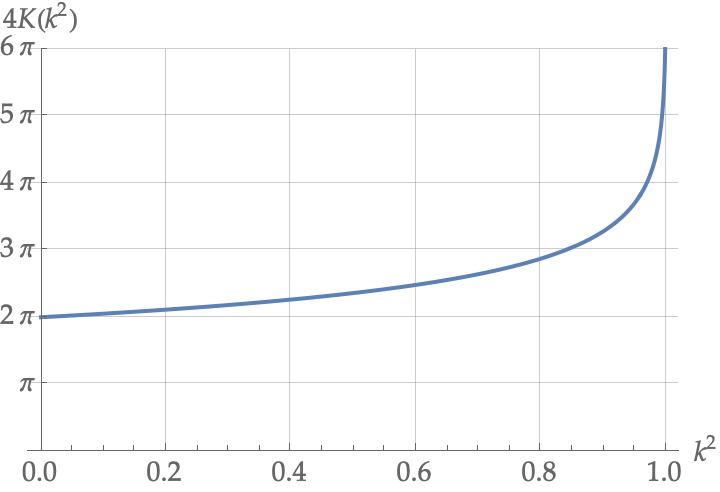
Figure 1: The k2superscript𝑘2k^{2}-dependence of K=K​(k2)đŸđŸsuperscript𝑘2K=K(k^{2}), the complete elliptical integral of the first kind. Shown is the graph for 4​K4đŸ4K, which is the period of sn​(u,k)sn𝑱𝑘\mathrm{sn}(u,k) and cn​(u,k)cn𝑱𝑘\mathrm{cn}(u,k) in u𝑱u. Note that Kâ†’âˆžâ†’đŸK\to\infty as k2→1→superscript𝑘21k^{2}\to 1.
Refer to caption
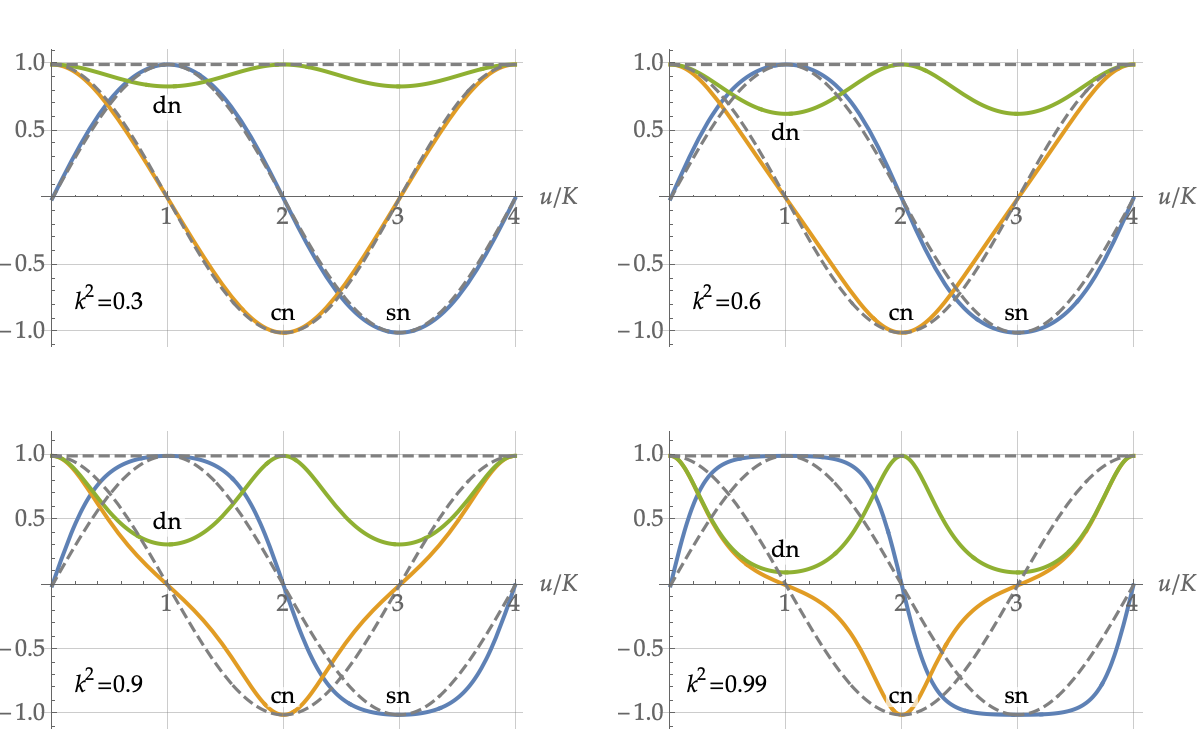
Figure 2: The u𝑱u-dependence of the Jacobi elliptical functions sn​(u,k)sn𝑱𝑘\mathrm{sn}(u,k), cn​(u,k)cn𝑱𝑘\mathrm{cn}(u,k), and dn​(u,k)dn𝑱𝑘\mathrm{dn}(u,k) for k2=0.3superscript𝑘20.3k^{2}=0.3 (upper left), k2=0.6superscript𝑘20.6k^{2}=0.6 (upper right), k2=0.9superscript𝑘20.9k^{2}=0.9 (lower left), and k2=0.99superscript𝑘20.99k^{2}=0.99 (lower right). The horizontal axis is in units of K=K​(k2)đŸđŸsuperscript𝑘2K=K(k^{2}), the complete elliptical integral of the first kind. The dashed lines are the k2=0superscript𝑘20k^{2}=0 case where sn​(u,0)=sin⁥usn𝑱0𝑱\mathrm{sn}(u,0)=\sin u, cn​(u,0)=cos⁥ucn𝑱0𝑱\mathrm{cn}(u,0)=\cos u, dn​(u,0)=1dn𝑱01\mathrm{dn}(u,0)=1.

III.1 Deformation of Quantum Mechanics into a theory of Asymmetric Tops

The deformation of canonical QM discussed in Refs. [2, 1] can be summarized as follows: The xđ‘„x-ponent, which is a map from S1superscript𝑆1S^{1} to S1superscript𝑆1S^{1} in canonical QM, is deformed to a map from S1superscript𝑆1S^{1} to S2superscript𝑆2S^{2} as:

x→​(Ξ)=[cos⁥Ξsin⁥Ξ]→X→​(Ξ|k,Ο)=[cΟ​cn​(2​K​ξ/π,k)cΟ2+sΟ2​k2​sn​(2​K​ξ/π,k)−sΟ​dn​(2​K​ξ/π,k)],formulae-sequenceâ†’đ‘„đœƒmatrix𝜃𝜃→→𝑋conditional𝜃𝑘𝜉matrixsubscript𝑐𝜉cn2đŸđœƒđœ‹đ‘˜superscriptsubscript𝑐𝜉2superscriptsubscript𝑠𝜉2superscript𝑘2sn2đŸđœƒđœ‹đ‘˜subscript𝑠𝜉dn2đŸđœƒđœ‹đ‘˜\vec{x}(\theta)=\begin{bmatrix}\cos\theta\\ \sin\theta\end{bmatrix}\qquad\to\qquad\vec{X}(\theta|k,\xi)=\begin{bmatrix}c_{\xi}\;\mathrm{cn}(2K\theta/\pi,k)\vphantom{\Big{|}}\\ \sqrt{c_{\xi}^{2}+s_{\xi}^{2}k^{2}}\;\mathrm{sn}(2K\theta/\pi,k)\\ -s_{\xi}\;\mathrm{dn}(2K\theta/\pi,k)\vphantom{\Big{|}}\end{bmatrix}\;, (46)

where cn​(u,k)cn𝑱𝑘\mathrm{cn}(u,k), sn​(u,k)sn𝑱𝑘\mathrm{sn}(u,k), dn​(u,k)dn𝑱𝑘\mathrm{dn}(u,k), with 0≀k<10𝑘10\leq k<1, are Jacobi’s elliptical functions [37]333 In the literature, Jacobi’s elliptical functions are also written as cn​(u,m)cn𝑱𝑚\mathrm{cn}(u,m), sn​(u,m)sn𝑱𝑚\mathrm{sn}(u,m), and dn​(u,m)dn𝑱𝑚\mathrm{dn}(u,m) with m=k2𝑚superscript𝑘2m=k^{2}, so care is necessary when comparing formulae. The functions JacobiCN[u,m], JacobiSN[u,m], JacobiDN[u,m] on Mathematica also adopt this definition. , and cΟ=cosâĄÎŸsubscript𝑐𝜉𝜉c_{\xi}=\cos\xi, sΟ=sinâĄÎŸsubscript𝑠𝜉𝜉s_{\xi}=\sin\xi, where 0≀Ο≀π/20𝜉𝜋20\leq\xi\leq\pi/2 is the second deformation parameter. The reason for the minus sign on the third component is explained later. Note that Jacobi’s elliptical functions satisfy the relations

cn2​(u,k)+sn2​(u,k)superscriptcn2𝑱𝑘superscriptsn2𝑱𝑘\displaystyle\mathrm{cn}^{2}(u,k)+\mathrm{sn}^{2}(u,k) =\displaystyle= 1,1\displaystyle 1\;,\vphantom{\big{|}} (47)
k2​sn2​(u,k)+dn2​(u,k)superscript𝑘2superscriptsn2𝑱𝑘superscriptdn2𝑱𝑘\displaystyle k^{2}\mathrm{sn}^{2}(u,k)+\mathrm{dn}^{2}(u,k) =\displaystyle= 1,1\displaystyle 1\;,\vphantom{\big{|}} (48)

so X→​(Ξ|k,Ο)→𝑋conditional𝜃𝑘𝜉\vec{X}(\theta|k,\xi) has unit norm.

The periods of cn​(u,k)cn𝑱𝑘\mathrm{cn}(u,k) and sn​(u,k)sn𝑱𝑘\mathrm{sn}(u,k) for real u𝑱u is 4​K4đŸ4K while that of dn​(u,k)dn𝑱𝑘\mathrm{dn}(u,k) is 2​K2đŸ2K, where K=K​(k2)đŸđŸsuperscript𝑘2K=K(k^{2}) is the complete elliptical integral of the first kind [37]. See FIGS. 1 and 2. In the above map, the arguments of the elliptical functions are rescaled so that the period in ξ𝜃\theta is 2​π2𝜋2\pi for cncn\mathrm{cn} and snsn\mathrm{sn}, and Ï€đœ‹\pi for dndn\mathrm{dn}. For latter convenience, we introduce the notation

Cn​(Ξ,k)≡cn​(2​K​ξ/π,k),Sn​(Ξ,k)≡sn​(2​K​ξ/π,k),Dn​(Ξ,k)≡dn​(2​K​ξ/π,k),formulae-sequenceCn𝜃𝑘cn2đŸđœƒđœ‹đ‘˜formulae-sequenceSn𝜃𝑘sn2đŸđœƒđœ‹đ‘˜Dn𝜃𝑘dn2đŸđœƒđœ‹đ‘˜\mathrm{Cn}(\theta,k)\,\equiv\,\mathrm{cn}(2K\theta/\pi,k)\;,\qquad\mathrm{Sn}(\theta,k)\,\equiv\,\mathrm{sn}(2K\theta/\pi,k)\;,\qquad\mathrm{Dn}(\theta,k)\,\equiv\,\mathrm{dn}(2K\theta/\pi,k)\;, (49)

to refer to these functions with their arguments rescaled. Due to the period of Dn​(Ξ)Dn𝜃\mathrm{Dn}(\theta) being Ï€đœ‹\pi instead of 2​π2𝜋2\pi, a phase shift by Ï€đœ‹\pi does not change the sign of X→​(Ξ|k,Ο)→𝑋conditional𝜃𝑘𝜉\vec{X}(\theta|k,\xi):

X→​(Ξ+π|k,Ο)≠−X→​(Ξ|k,Ο),→𝑋𝜃conditional𝜋𝑘𝜉→𝑋conditional𝜃𝑘𝜉\vec{X}(\theta+\pi|k,\xi)\;\neq\;-\vec{X}(\theta|k,\xi)\;, (50)

except when Ο=0𝜉0\xi=0 in which case the third component of X→​(Ξ|k,0)→𝑋conditional𝜃𝑘0\vec{X}(\theta|k,0) is missing. To allow for a sign flip, we let the magnitudes of the coefficients be negative as well as positive.
Refer to caption
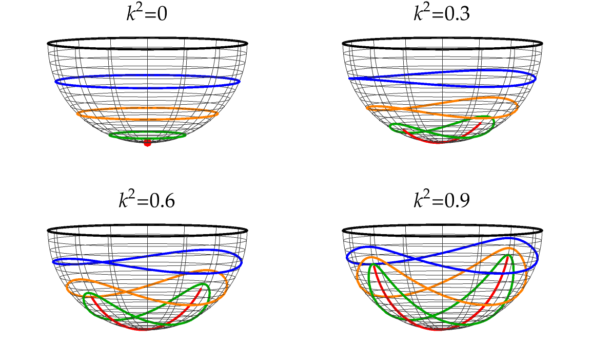
Figure 3: Phase trajectories on S2superscript𝑆2S^{2} in Nambu QM for positive amplitudes. Only the southern hemisphere is shown. Trajectories in the northern hemisphere occur when the amplitude is negative. The colored lines in each figure indicate Ο=0𝜉0\xi=0 (Black), Ο=π/8𝜉𝜋8\xi=\pi/8 (Blue), Ο=π/4𝜉𝜋4\xi=\pi/4 (Orange), Ο=3​π/8𝜉3𝜋8\xi=3\pi/8 (Green), and Ο=π/2𝜉𝜋2\xi=\pi/2 (Red). When Ο=0𝜉0\xi=0, the trajectory always follows the equator regardless of the value of k𝑘k. However, the phase time-evolves with uniform angular velocity along the equator only when k=0𝑘0k=0. When k=0𝑘0k=0 and Ο=π/2𝜉𝜋2\xi=\pi/2, the phase is stationary at the south pole.

The dependence of the trajectory of X→​(Ξ|k,Ο)→𝑋conditional𝜃𝑘𝜉\vec{X}(\theta|k,\xi) on S2superscript𝑆2S^{2} on the deformation parameters k𝑘k and ÎŸđœ‰\xi is shown FIG. 3. For instance, when k=0𝑘0k=0 the trajectory reduces to

X→​(Ξ|0,Ο)=[cΟ​x→​(Ξ)−sΟ]=[cΟ​cos⁥ΞcΟ​sin⁡ξ−sΟ],→𝑋conditional𝜃0𝜉matrixsubscriptđ‘đœ‰â†’đ‘„đœƒsubscript𝑠𝜉matrixsubscript𝑐𝜉𝜃subscript𝑐𝜉𝜃subscript𝑠𝜉\vec{X}(\theta|0,\xi)\;=\;\begin{bmatrix}c_{\xi}\vec{x}(\theta)\\ -s_{\xi}\end{bmatrix}\;=\;\begin{bmatrix}c_{\xi}\cos\theta\\ c_{\xi}\sin\theta\\ -s_{\xi}\end{bmatrix}\;, (51)

namely, the path of constant latitude âˆ’ÎŸđœ‰-\xi on S2superscript𝑆2S^{2}. When Ο=0𝜉0\xi=0 this will be the equator, whereas when Ο=π/2𝜉𝜋2\xi=\pi/2 this will be the south pole. Setting Ο=0𝜉0\xi=0 for a non-zero k𝑘k would lead to

X→​(ξ|k,0)=[Cn​(ξ,k)Sn​(ξ,k)0],→𝑋conditional𝜃𝑘0matrixCn𝜃𝑘Sn𝜃𝑘0\vec{X}(\theta|k,0)\;=\;\begin{bmatrix}\mathrm{Cn}(\theta,k)\\ \mathrm{Sn}(\theta,k)\\ 0\end{bmatrix}\;, (52)

which traces the equator of S2superscript𝑆2S^{2} but with a non-canonical dependence on ξ𝜃\theta.

The coefficients of the n𝑛nth energy eigenstate will time-evolve as

ι→n​(t)=An​X→​(−ωn​(t−tn)|kn,Οn)=An​[cΟn​Cn​(ωn​(t−tn),kn)−cΟn2+sΟn2​kn2​Sn​(ωn​(t−tn),kn)−sΟn​Dn​(ωn​(t−tn),kn)],subscript→ι𝑛𝑡subscript𝐮𝑛→𝑋conditionalsubscript𝜔𝑛𝑡subscript𝑡𝑛subscript𝑘𝑛subscript𝜉𝑛subscript𝐮𝑛matrixsubscript𝑐subscript𝜉𝑛Cnsubscript𝜔𝑛𝑡subscript𝑡𝑛subscript𝑘𝑛superscriptsubscript𝑐subscript𝜉𝑛2superscriptsubscript𝑠subscript𝜉𝑛2superscriptsubscript𝑘𝑛2Snsubscript𝜔𝑛𝑡subscript𝑡𝑛subscript𝑘𝑛subscript𝑠subscript𝜉𝑛Dnsubscript𝜔𝑛𝑡subscript𝑡𝑛subscript𝑘𝑛\vec{\Psi}_{n}(t)\;=\;A_{n}\,\vec{X}(-\omega_{n}(t-t_{n})|k_{n},\xi_{n})\;=\;A_{n}\begin{bmatrix}\phantom{-}c_{\xi_{n}}\mathrm{Cn}(\omega_{n}(t-t_{n}),k_{n})\vphantom{\Big{|}}\\ -\sqrt{c_{\xi_{n}}^{2}+s_{\xi_{n}}^{2}k_{n}^{2}}\;\mathrm{Sn}(\omega_{n}(t-t_{n}),k_{n})\\ -s_{\xi_{n}}\mathrm{Dn}(\omega_{n}(t-t_{n}),k_{n})\vphantom{\Big{|}}\end{bmatrix}, (53)

where tnsubscript𝑡𝑛t_{n} sets the initial condition for each n𝑛n. Note that when Ο=0𝜉0\xi=0 the trajectory of X→​(−ω​t|k,0)→𝑋conditional𝜔𝑡𝑘0\vec{X}(-\omega t|k,0) will be along the equator of S2superscript𝑆2S^{2}, but it will not time-evolve with constant angular velocity Ï‰đœ”\omega except for the canonical QM case k=0𝑘0k=0.

The trajectory of ι→n​(t)subscript→ι𝑛𝑡\vec{\Psi}_{n}(t) on S2superscript𝑆2S^{2} is that of the angular momentum of a free asymmetric top in the frame fixed to itself. There, the angular momentum

A2=L12+L22+L32,superscript𝐮2superscriptsubscript𝐿12superscriptsubscript𝐿22superscriptsubscript𝐿32A^{2}\;=\;L_{1}^{2}+L_{2}^{2}+L_{3}^{2}\;, (54)

and energy

E=L122​I1+L222​I2+L322​I3,𝐾superscriptsubscript𝐿122subscriptđŒ1superscriptsubscript𝐿222subscriptđŒ2superscriptsubscript𝐿322subscriptđŒ3E\;=\;\dfrac{L_{1}^{2}}{2I_{1}}+\dfrac{L_{2}^{2}}{2I_{2}}+\dfrac{L_{3}^{2}}{2I_{3}}\;, (55)

are both fixed so the angular momentum vector will evolve along the intersection of the two surfaces A2=superscript𝐮2absentA^{2}=constant and E=𝐾absentE=constant. k=0𝑘0k=0 corresponds to the symmetric top with I1=I2subscriptđŒ1subscriptđŒ2I_{1}=I_{2}. However, the dynamics we chose in Eq. (53) is not that of the asymmetric top. Indeed, when the intersection of the two surfaces is the equator, Ο=0𝜉0\xi=0, the angular momentum of the asymmetric (symmetric at the equator) top stays fixed and does not time evolve. This must be the case since the Ο=0𝜉0\xi=0 limit must correspond to the same physical configuration for the top regardless of the value of k𝑘k. See Appendix A.3 for details. Our dynamics here is chosen so that k=0𝑘0k=0 and Ο=0𝜉0\xi=0 recovers canonical QM. The only thing that is maintained is the direction of evolution along the trajectory, by the choice of the sign of the third component.

Note that this is but one way to generate a closed path on S2superscript𝑆2S^{2}. Other deformations of the xđ‘„x-ponent are possible, each leading to different generalizations of canonical QM. However, we will not dwell on this question further in this paper.

III.2 Inner Product

We extend the inner product of two states to the quaternion

⟹Ω|Κ⟩=g​(Ί,Κ)−i​Δ1​(Ί,Κ)−j​Δ2​(Ί,Κ)−k​Δ3​(Ί,Κ),inner-productΩι𝑔Ωι𝑖subscript𝜀1Ωι𝑗subscript𝜀2Ωι𝑘subscript𝜀3ΊΚ\langle\Phi|\Psi\rangle\;=\;g(\Phi,\Psi)-i\,\varepsilon_{1}(\Phi,\Psi)-j\,\varepsilon_{2}(\Phi,\Psi)-k\,\varepsilon_{3}(\Phi,\Psi)\;, (56)

where

g​(Ω,ι)𝑔Ωι\displaystyle g(\Phi,\Psi) =\displaystyle= ∑n(Ω→n⋅ι→n),subscript𝑛⋅subscript→Ω𝑛subscript→ι𝑛\displaystyle\sum_{n}(\vec{\Phi}_{n}\cdot\vec{\Psi}_{n})\;,\vphantom{\bigg{|}} (57)
Δ→​(Ί,Κ)→𝜀Ωι\displaystyle\vec{\varepsilon}\,(\Phi,\Psi) =\displaystyle= [Δ1​(Ί,Κ)Δ2​(Ί,Κ)Δ3​(Ί,Κ)]=∑n(Ω→n×ι→n).matrixsubscript𝜀1ΊΚsubscript𝜀2ΊΚsubscript𝜀3ΊΚsubscript𝑛subscript→Ω𝑛subscript→ι𝑛\displaystyle\begin{bmatrix}\varepsilon_{1}(\Phi,\Psi)\\ \varepsilon_{2}(\Phi,\Psi)\\ \varepsilon_{3}(\Phi,\Psi)\end{bmatrix}\;=\;\sum_{n}(\vec{\Phi}_{n}\times\vec{\Psi}_{n})\;.\vphantom{\bigg{|}} (58)

The dot and cross products are now defined in three dimensions. This inner product results if we map the 3D phase vector ι→→ι\vec{\Psi} to a purely imaginary quaternion

ι→=[ι1ι2ι3]→ι=i​ι1+j​ι2+k​ι3,formulae-sequence→ιmatrixsubscriptι1subscriptι2subscriptι3→ι𝑖subscriptι1𝑗subscriptι2𝑘subscriptι3\vec{\Psi}\,=\,\begin{bmatrix}\Psi_{1}\\ \Psi_{2}\\ \Psi_{3}\end{bmatrix}\qquad\to\qquad\Psi\,=\,i\Psi_{1}+j\Psi_{2}+k\Psi_{3}\;, (59)

and define the inner product to be

⟹Ω|Κ⟩inner-productΊΚ\displaystyle\langle\Phi|\Psi\rangle =\displaystyle= Ω¯​ι=−(i​Ω1+j​Ω2+k​Ω3)​(i​ι1+j​ι2+k​ι3).¯Ωι𝑖subscriptΊ1𝑗subscriptΊ2𝑘subscriptΊ3𝑖subscriptΚ1𝑗subscriptΚ2𝑘subscriptΚ3\displaystyle\overline{\Phi}\Psi\;=\;-(i\Phi_{1}+j\Phi_{2}+k\Phi_{3})(i\Psi_{1}+j\Psi_{2}+k\Psi_{3})\;. (60)

Note that

⟹ι|Κ⟩=g​(Κ,Κ)=∑nAn2,inner-productιι𝑔ιιsubscript𝑛superscriptsubscript𝐮𝑛2\langle\Psi|\Psi\rangle\;=\;g(\Psi,\Psi)\;=\;\sum_{n}A_{n}^{2}\;, (61)

and

|⟹Ω|Κ⟩|2=g​(Ί,Κ)2+Δ→​(Ί,Κ)⋅Δ→​(Ί,Κ).superscriptinner-productΊΚ2𝑔superscriptΊΚ2⋅→𝜀Ωι→𝜀Ωι|\langle\Phi|\Psi\rangle|^{2}\;=\;g(\Phi,\Psi)^{2}+\vec{\varepsilon}\,(\Phi,\Psi)\cdot\vec{\varepsilon}\,(\Phi,\Psi)\;. (62)

If we write

(Ω→n⋅ι→n)=Cn​cos⁥ζn,(Ω→n×ι→n)=C→n​sin⁥ζn,formulae-sequence⋅subscript→Ω𝑛subscript→ι𝑛subscriptđ¶đ‘›subscript𝜁𝑛subscript→Ω𝑛subscript→ι𝑛subscriptâ†’đ¶đ‘›subscript𝜁𝑛(\vec{\Phi}_{n}\cdot\vec{\Psi}_{n})\;=\;C_{n}\cos\zeta_{n}\;,\qquad(\vec{\Phi}_{n}\times\vec{\Psi}_{n})\;=\;\vec{C}_{n}\sin\zeta_{n}\;, (63)

where |C→n|=Cnsubscriptâ†’đ¶đ‘›subscriptđ¶đ‘›|\vec{C}_{n}|=C_{n}, then

|⟹Ω|Κ⟩|2superscriptinner-productΊΚ2\displaystyle|\langle\Phi|\Psi\rangle|^{2} =\displaystyle= ∑n∑m(Cn​Cm​cos⁥ζn​cos⁥ζm+C→n⋅C→m​sin⁥ζn​sin⁥ζm)subscript𝑛subscript𝑚subscriptđ¶đ‘›subscriptđ¶đ‘šsubscript𝜁𝑛subscript𝜁𝑚⋅subscriptâ†’đ¶đ‘›subscriptâ†’đ¶đ‘šsubscript𝜁𝑛subscript𝜁𝑚\displaystyle\sum_{n}\sum_{m}\Big{(}C_{n}C_{m}\cos\zeta_{n}\cos\zeta_{m}+\vec{C}_{n}\cdot\vec{C}_{m}\sin\zeta_{n}\sin\zeta_{m}\Big{)} (64)
=\displaystyle= ∑nCn2⏟P​(n)+∑n<m2​Cn​Cm​(cos⁥ζn​cos⁥ζm+cos⁥γn​m​sin⁥ζn​sin⁥ζm)⏟I2​(n,m),subscript𝑛subscript⏟superscriptsubscriptđ¶đ‘›2𝑃𝑛subscript𝑛𝑚subscript⏟2subscriptđ¶đ‘›subscriptđ¶đ‘šsubscript𝜁𝑛subscript𝜁𝑚subscriptđ›Ÿđ‘›đ‘šsubscript𝜁𝑛subscript𝜁𝑚subscriptđŒ2𝑛𝑚\displaystyle\sum_{n}\underbrace{C_{n}^{2}}_{\displaystyle P(n)}+\sum_{n<m}\underbrace{2C_{n}C_{m}\Big{(}\cos\zeta_{n}\cos\zeta_{m}+\cos\gamma_{nm}\sin\zeta_{n}\sin\zeta_{m}\Big{)}}_{\displaystyle I_{2}(n,m)}\;, (65)

where Îłn​msubscriptđ›Ÿđ‘›đ‘š\gamma_{nm} is the angle between C→nsubscriptâ†’đ¶đ‘›\vec{C}_{n} and C→msubscriptâ†’đ¶đ‘š\vec{C}_{m}. Unlike the canonical QM case, cf. Eq. (19), the interference I2​(n,m)subscriptđŒ2𝑛𝑚I_{2}(n,m) will depend on the sum ζn+ζmsubscript𝜁𝑛subscript𝜁𝑚\zeta_{n}+\zeta_{m} as well as the difference ζn−ζmsubscript𝜁𝑛subscript𝜁𝑚\zeta_{n}-\zeta_{m} unless cos⁥γn​m=1subscriptđ›Ÿđ‘›đ‘š1\cos\gamma_{nm}=1.

The angle ζnsubscript𝜁𝑛\zeta_{n} defined in Eq. (63) is invariant under 3D rotations of the n𝑛nth S2superscript𝑆2S^{2} phase manifold associated with the n𝑛nth energy eigenstate, generalizing the canonical case which was invariant under 2D rotations of the S1superscript𝑆1S^{1} phase manifold. Note, however, that in general, a phase shift of an energy eigenstate

|n⟩→X→​(αn|kn,Οn)​|n⟩ket𝑛→→𝑋conditionalsubscriptđ›Œđ‘›subscript𝑘𝑛subscript𝜉𝑛ket𝑛\big{|}n\big{\rangle}\quad\to\quad\vec{X}(\alpha_{n}|k_{n},\xi_{n})\big{|}n\big{\rangle} (66)

does not correspond to a 3D rotation of S2superscript𝑆2S^{2}, except for the symmetric top case kn=0subscript𝑘𝑛0k_{n}=0, in which case this phase shift becomes a rotation of angle Î±đ›Œ\alpha around the north-south axis of S2superscript𝑆2S^{2}. Thus, to maintain the invariance of the angles ζnsubscript𝜁𝑛\zeta_{n}, and consequently that of the inner product ⟹Ω|Κ⟩inner-productΊΚ\langle\Phi|\Psi\rangle under phase shifts of the individual energy eigenstates, we must choose kn=0subscript𝑘𝑛0k_{n}=0 for all n𝑛n. Even then, we do not have the freedom to shift the phases of different states, i.e. different linear combinations of the energy eigenstates, independently since |⟹Ω|Κ⟩|2superscriptinner-productΊΚ2|\langle\Phi|\Psi\rangle|^{2} will not remain invariant. So the projective nature of the state space is lost.

This difference between the inner products in canonical QM and Nambu QM has consequences in oscillation phenomena. We demonstrate this using the calculation of neutrino oscillation probabilities next, allowing kn≠0subscript𝑘𝑛0k_{n}\neq 0 to see their effect.

III.3 Neutrino Oscillations in Nambu QM

As an example of oscillation phenomena, we calculate the two-flavor neutrino oscillation probabilities. For simplicity, we take the deformation parameters knsubscript𝑘𝑛k_{n} and Οnsubscript𝜉𝑛\xi_{n} to be the same for all energy eigenstates.

Let the flavor eigenstates |A⟩ket𝐮\big{|}A\big{\rangle} and |B⟩ketđ”\big{|}B\big{\rangle} be given by superpositions of mass eigenstates |1⟩ket1\big{|}1\big{\rangle} and |2⟩ket2\big{|}2\big{\rangle} as

|A⟩ket𝐮\displaystyle\big{|}A\big{\rangle} =\displaystyle= cξ​|1⟩+sξ​|2⟩,subscript𝑐𝜃ket1subscript𝑠𝜃ket2\displaystyle\phantom{+}c_{\theta}\big{|}1\big{\rangle}+s_{\theta}\big{|}2\big{\rangle}\;,\vphantom{\Big{|}} (67)
|B⟩ketđ”\displaystyle\big{|}B\big{\rangle} =\displaystyle= −sξ​|1⟩+cξ​|2⟩.subscript𝑠𝜃ket1subscript𝑐𝜃ket2\displaystyle-s_{\theta}\big{|}1\big{\rangle}+c_{\theta}\big{|}2\big{\rangle}\;.\vphantom{\Big{|}} (68)

Then,

A→1=cξ​X→​(0),A→2=sξ​X→​(0),B→1=−sξ​X→​(0),B→2=cξ​X→​(0),formulae-sequencesubscript→𝐮1subscript𝑐𝜃→𝑋0formulae-sequencesubscript→𝐮2subscript𝑠𝜃→𝑋0formulae-sequencesubscriptâ†’đ”1subscript𝑠𝜃→𝑋0subscriptâ†’đ”2subscript𝑐𝜃→𝑋0\vec{A}_{1}\;=\;c_{\theta}\,\vec{X}(0)\;,\qquad\vec{A}_{2}\;=\;s_{\theta}\,\vec{X}(0)\;,\qquad\vec{B}_{1}\;=\;-s_{\theta}\,\vec{X}(0)\;,\qquad\vec{B}_{2}\;=\;c_{\theta}\,\vec{X}(0)\;, (69)

where

X→​(0)=X→​(0|k,Ο)=[cΟ0−sΟ]→𝑋0→𝑋conditional0𝑘𝜉matrixsubscript𝑐𝜉0subscript𝑠𝜉\vec{X}(0)\;=\;\vec{X}(0|k,\xi)\;=\;\begin{bmatrix}c_{\xi}\\ 0\\ -s_{\xi}\end{bmatrix} (70)

represents a “phaseless” state. Let |ι​(0)⟩=|A⟩ketΚ0ket𝐮\big{|}\Psi(0)\big{\rangle}=\big{|}A\big{\rangle}, that is:

ι→1​(0)=A→1=cξ​X→​(0),ι→2​(0)=A→2=sξ​X→​(0).formulae-sequencesubscript→ι10subscript→𝐮1subscript𝑐𝜃→𝑋0subscript→ι20subscript→𝐮2subscript𝑠𝜃→𝑋0\vec{\Psi}_{1}(0)\;=\;\vec{A}_{1}\;=\;c_{\theta}\,\,\vec{X}(0)\;,\qquad\vec{\Psi}_{2}(0)\;=\;\vec{A}_{2}\;=\;s_{\theta}\,\,\vec{X}(0)\;. (71)

At a later time t𝑡t, we have

ι→1​(t)=cξ​X→​(−ω1​t),ι→2​(t)=sξ​X→​(−ω2​t),formulae-sequencesubscript→ι1𝑡subscript𝑐𝜃→𝑋subscript𝜔1𝑡subscript→ι2𝑡subscript𝑠𝜃→𝑋subscript𝜔2𝑡\vec{\Psi}_{1}(t)\;=\;c_{\theta}\,\,\vec{X}(-\omega_{1}t)\;,\qquad\vec{\Psi}_{2}(t)\;=\;s_{\theta}\,\vec{X}(-\omega_{2}t)\;, (72)

where

X→​(−ωi​t)=X→​(−ωi​t|k,Ο)=[cΟ​Cn​(ωi​t,k)−Îș​cΟ​Sn​(ωi​t,k)−sΟ​Dn​(ωi​t,k)]=[cΟ​Cni−Îș​cΟ​Sni−sΟ​Dni].→𝑋subscript𝜔𝑖𝑡→𝑋conditionalsubscript𝜔𝑖𝑡𝑘𝜉matrixsubscript𝑐𝜉Cnsubscript𝜔𝑖𝑡𝑘𝜅subscript𝑐𝜉Snsubscript𝜔𝑖𝑡𝑘subscript𝑠𝜉Dnsubscript𝜔𝑖𝑡𝑘matrixsubscript𝑐𝜉subscriptCn𝑖𝜅subscript𝑐𝜉subscriptSn𝑖subscript𝑠𝜉subscriptDn𝑖\vec{X}(-\omega_{i}t)\;=\;\vec{X}(-\omega_{i}t|k,\xi)\;=\;\begin{bmatrix}c_{\xi}\,\mathrm{Cn}(\omega_{i}t,k)\\ -\kappa c_{\xi}\,\mathrm{Sn}(\omega_{i}t,k)\\ -s_{\xi}\,\mathrm{Dn}(\omega_{i}t,k)\end{bmatrix}\;=\;\begin{bmatrix}c_{\xi}\,\mathrm{Cn}_{i}\\ -\kappa c_{\xi}\,\mathrm{Sn}_{i}\\ -s_{\xi}\,\mathrm{Dn}_{i}\end{bmatrix}\;. (73)

Here, we use the shorthand

Îș=1+k2​tan2âĄÎŸ,Sni=Sn​(ωi​t,k),Cni=Cn​(ωi​t,k),Dni=Dn​(ωi​t,k).formulae-sequence𝜅1superscript𝑘2superscript2𝜉formulae-sequencesubscriptSn𝑖Snsubscript𝜔𝑖𝑡𝑘formulae-sequencesubscriptCn𝑖Cnsubscript𝜔𝑖𝑡𝑘subscriptDn𝑖Dnsubscript𝜔𝑖𝑡𝑘\kappa\,=\,\sqrt{1+k^{2}\tan^{2}\xi}\;,\quad\mathrm{Sn}_{i}\,=\,\mathrm{Sn}(\omega_{i}t,k)\;,\quad\mathrm{Cn}_{i}\,=\,\mathrm{Cn}(\omega_{i}t,k)\;,\quad\mathrm{Dn}_{i}\,=\,\mathrm{Dn}(\omega_{i}t,k)\;. (74)

Then, the symmetric parts of ⟹A|ι​(t)⟩inner-product𝐮ι𝑡\langle A|\Psi(t)\rangle and ⟹B|ι​(t)⟩inner-productđ”Îšđ‘Ą\langle B|\Psi(t)\rangle are

g​(A,ι​(t))𝑔𝐮ι𝑡\displaystyle g(A,\Psi(t)) =\displaystyle= A→1⋅ι→1​(t)+A→2⋅ι→2​(t)⋅subscript→𝐮1subscript→ι1𝑡⋅subscript→𝐮2subscript→ι2𝑡\displaystyle\vec{A}_{1}\cdot\vec{\Psi}_{1}(t)+\vec{A}_{2}\cdot\vec{\Psi}_{2}(t)\vphantom{\bigg{|}} (75)
=\displaystyle= cΞ2​X→​(0)⋅X→​(−ω1​t)+sΞ2​X→​(0)⋅X→​(−ω2​t)⋅superscriptsubscript𝑐𝜃2→𝑋0→𝑋subscript𝜔1𝑡⋅superscriptsubscript𝑠𝜃2→𝑋0→𝑋subscript𝜔2𝑡\displaystyle c_{\theta}^{2}\,\vec{X}(0)\cdot\vec{X}(-\omega_{1}t)+s_{\theta}^{2}\,\vec{X}(0)\cdot\vec{X}(-\omega_{2}t)\vphantom{\bigg{|}} (76)
=\displaystyle= cΞ2​(cΟ2​Cn1+sΟ2​Dn1)+sΞ2​(cΟ2​Cn2+sΟ2​Dn2),superscriptsubscript𝑐𝜃2superscriptsubscript𝑐𝜉2subscriptCn1superscriptsubscript𝑠𝜉2subscriptDn1superscriptsubscript𝑠𝜃2superscriptsubscript𝑐𝜉2subscriptCn2superscriptsubscript𝑠𝜉2subscriptDn2\displaystyle c_{\theta}^{2}\Bigl{(}\,c_{\xi}^{2}\,\mathrm{Cn}_{1}+s_{\xi}^{2}\,\mathrm{Dn}_{1}\,\Bigr{)}+s_{\theta}^{2}\Bigl{(}\,c_{\xi}^{2}\,\mathrm{Cn}_{2}+s_{\xi}^{2}\,\mathrm{Dn}_{2}\,\Bigr{)}\;,\vphantom{\bigg{|}} (77)
g​(B,ι​(t))đ‘”đ”Îšđ‘Ą\displaystyle g(B,\Psi(t)) =\displaystyle= B→1⋅ι→1​(t)+B→2⋅ι→2​(t)⋅subscriptâ†’đ”1subscript→ι1𝑡⋅subscriptâ†’đ”2subscript→ι2𝑡\displaystyle\vec{B}_{1}\cdot\vec{\Psi}_{1}(t)+\vec{B}_{2}\cdot\vec{\Psi}_{2}(t)\vphantom{\bigg{|}} (78)
=\displaystyle= −sξ​cξ​X→​(0)⋅X→​(−ω1​t)+sξ​cξ​X→​(0)⋅X→​(−ω2​t)⋅subscript𝑠𝜃subscript𝑐𝜃→𝑋0→𝑋subscript𝜔1𝑡⋅subscript𝑠𝜃subscript𝑐𝜃→𝑋0→𝑋subscript𝜔2𝑡\displaystyle-s_{\theta}c_{\theta}\,\vec{X}(0)\cdot\vec{X}(-\omega_{1}t)+s_{\theta}c_{\theta}\,\vec{X}(0)\cdot\vec{X}(-\omega_{2}t)\vphantom{\bigg{|}} (79)
=\displaystyle= −sξ​cξ​(cΟ2​Cn1+sΟ2​Dn1)+sξ​cξ​(cΟ2​Cn2+sΟ2​Dn2).subscript𝑠𝜃subscript𝑐𝜃superscriptsubscript𝑐𝜉2subscriptCn1superscriptsubscript𝑠𝜉2subscriptDn1subscript𝑠𝜃subscript𝑐𝜃superscriptsubscript𝑐𝜉2subscriptCn2superscriptsubscript𝑠𝜉2subscriptDn2\displaystyle-s_{\theta}c_{\theta}\Bigl{(}\,c_{\xi}^{2}\,\mathrm{Cn}_{1}+s_{\xi}^{2}\,\mathrm{Dn}_{1}\,\Bigr{)}+s_{\theta}c_{\theta}\Bigl{(}\,c_{\xi}^{2}\,\mathrm{Cn}_{2}+s_{\xi}^{2}\,\mathrm{Dn}_{2}\,\Bigr{)}\;.\vphantom{\bigg{|}} (80)

while the antisymmetric parts of ⟹A|ι​(t)⟩inner-product𝐮ι𝑡\langle A|\Psi(t)\rangle and ⟹B|ι​(t)⟩inner-productđ”Îšđ‘Ą\langle B|\Psi(t)\rangle are

Δ→​(A,ι​(t))→𝜀𝐮ι𝑡\displaystyle\vec{\varepsilon}\,(A,\Psi(t)) =\displaystyle= A→1×ι→1​(t)+A→2×ι→2​(t)subscript→𝐮1subscript→ι1𝑡subscript→𝐮2subscript→ι2𝑡\displaystyle\vec{A}_{1}\times\vec{\Psi}_{1}(t)+\vec{A}_{2}\times\vec{\Psi}_{2}(t) (81)
=\displaystyle= cΞ2​X→​(0)×X→​(−ω1​t)+sΞ2​X→​(0)×X→​(−ω2​t)superscriptsubscript𝑐𝜃2→𝑋0→𝑋subscript𝜔1𝑡superscriptsubscript𝑠𝜃2→𝑋0→𝑋subscript𝜔2𝑡\displaystyle c_{\theta}^{2}\,\vec{X}(0)\times\vec{X}(-\omega_{1}t)+s_{\theta}^{2}\,\vec{X}(0)\times\vec{X}(-\omega_{2}t)\vphantom{\bigg{|}} (82)
=\displaystyle= cΞ2​[−Îș​sΟ​cΟ​Sn1sΟ​cΟ​(Dn1−Cn1)−Îș​cΟ2​Sn1]+sΞ2​[−Îș​sΟ​cΟ​Sn2sΟ​cΟ​(Dn2−Cn2)−Îș​cΟ2​Sn2],superscriptsubscript𝑐𝜃2matrix𝜅subscript𝑠𝜉subscript𝑐𝜉subscriptSn1subscript𝑠𝜉subscript𝑐𝜉subscriptDn1subscriptCn1𝜅superscriptsubscript𝑐𝜉2subscriptSn1superscriptsubscript𝑠𝜃2matrix𝜅subscript𝑠𝜉subscript𝑐𝜉subscriptSn2subscript𝑠𝜉subscript𝑐𝜉subscriptDn2subscriptCn2𝜅superscriptsubscript𝑐𝜉2subscriptSn2\displaystyle c_{\theta}^{2}\begin{bmatrix}-\kappa s_{\xi}c_{\xi}\,\mathrm{Sn}_{1}\\ s_{\xi}c_{\xi}\bigl{(}\mathrm{Dn}_{1}-\mathrm{Cn}_{1}\bigr{)}\\ -\kappa c_{\xi}^{2}\,\mathrm{Sn}_{1}\end{bmatrix}+s_{\theta}^{2}\begin{bmatrix}-\kappa s_{\xi}c_{\xi}\,\mathrm{Sn}_{2}\\ s_{\xi}c_{\xi}\bigl{(}\mathrm{Dn}_{2}-\mathrm{Cn}_{2}\bigr{)}\\ -\kappa c_{\xi}^{2}\,\mathrm{Sn}_{2}\end{bmatrix}\;, (83)
Δ→​(B,ι​(t))â†’đœ€đ”Îšđ‘Ą\displaystyle\vec{\varepsilon}\,(B,\Psi(t)) =\displaystyle= B→1×ι→1​(t)+B→2×ι→2​(t)subscriptâ†’đ”1subscript→ι1𝑡subscriptâ†’đ”2subscript→ι2𝑡\displaystyle\vec{B}_{1}\times\vec{\Psi}_{1}(t)+\vec{B}_{2}\times\vec{\Psi}_{2}(t) (85)
=\displaystyle= −sξ​cξ​X→​(0)×X→​(−ω1​t)+sξ​cξ​X→​(0)×X→​(−ω2​t)subscript𝑠𝜃subscript𝑐𝜃→𝑋0→𝑋subscript𝜔1𝑡subscript𝑠𝜃subscript𝑐𝜃→𝑋0→𝑋subscript𝜔2𝑡\displaystyle-s_{\theta}c_{\theta}\;\vec{X}(0)\times\vec{X}(-\omega_{1}t)+s_{\theta}c_{\theta}\;\vec{X}(0)\times\vec{X}(-\omega_{2}t)\vphantom{\bigg{|}} (86)
=\displaystyle= −sξ​cξ​[−Îș​sΟ​cΟ​Sn1sΟ​cΟ​(Dn1−Cn1)−Îș​cΟ2​Sn1]+sξ​cξ​[−Îș​sΟ​cΟ​Sn2sΟ​cΟ​(Dn2−Cn2)−Îș​cΟ2​Sn2].subscript𝑠𝜃subscript𝑐𝜃matrix𝜅subscript𝑠𝜉subscript𝑐𝜉subscriptSn1subscript𝑠𝜉subscript𝑐𝜉subscriptDn1subscriptCn1𝜅superscriptsubscript𝑐𝜉2subscriptSn1subscript𝑠𝜃subscript𝑐𝜃matrix𝜅subscript𝑠𝜉subscript𝑐𝜉subscriptSn2subscript𝑠𝜉subscript𝑐𝜉subscriptDn2subscriptCn2𝜅superscriptsubscript𝑐𝜉2subscriptSn2\displaystyle-s_{\theta}c_{\theta}\begin{bmatrix}-\kappa s_{\xi}c_{\xi}\,\mathrm{Sn}_{1}\\ s_{\xi}c_{\xi}\bigl{(}\mathrm{Dn}_{1}-\mathrm{Cn}_{1}\bigr{)}\\ -\kappa c_{\xi}^{2}\,\mathrm{Sn}_{1}\end{bmatrix}+s_{\theta}c_{\theta}\begin{bmatrix}-\kappa s_{\xi}c_{\xi}\,\mathrm{Sn}_{2}\\ s_{\xi}c_{\xi}\bigl{(}\mathrm{Dn}_{2}-\mathrm{Cn}_{2}\bigr{)}\\ -\kappa c_{\xi}^{2}\,\mathrm{Sn}_{2}\end{bmatrix}\;. (87)

Therefore, the survival and transition probabilities are given by

P​(A→A)𝑃→𝐮𝐮\displaystyle P(A\to A) =\displaystyle= g​(A,ι​(t))2+Δ→​(A,ι​(t))⋅Δ→​(A,ι​(t))𝑔superscript𝐮ι𝑡2⋅→𝜀𝐮ι𝑡→𝜀𝐮ι𝑡\displaystyle g(A,\Psi(t))^{2}+\vec{\varepsilon}\,(A,\Psi(t))\cdot\vec{\varepsilon}\,(A,\Psi(t))\vphantom{\Big{|}} (88)
=\displaystyle= cΞ4+sΞ4+2​cΞ2​sΞ2​[cΟ2​(Sn1​Sn2+Cn1​Cn2)+sΟ2​(k2​Sn1​Sn2+Dn1​Dn2)]superscriptsubscript𝑐𝜃4superscriptsubscript𝑠𝜃42superscriptsubscript𝑐𝜃2superscriptsubscript𝑠𝜃2delimited-[]superscriptsubscript𝑐𝜉2subscriptSn1subscriptSn2subscriptCn1subscriptCn2superscriptsubscript𝑠𝜉2superscript𝑘2subscriptSn1subscriptSn2subscriptDn1subscriptDn2\displaystyle c_{\theta}^{4}+s_{\theta}^{4}+2c_{\theta}^{2}s_{\theta}^{2}\Bigl{[}c_{\xi}^{2}\big{(}\mathrm{Sn}_{1}\,\mathrm{Sn}_{2}+\mathrm{Cn}_{1}\,\mathrm{Cn}_{2}\bigr{)}+s_{\xi}^{2}\big{(}k^{2}\,\mathrm{Sn}_{1}\,\mathrm{Sn}_{2}+\mathrm{Dn}_{1}\,\mathrm{Dn}_{2}\bigr{)}\Bigr{]}\vphantom{\Big{|}} (89)
=\displaystyle= 1−sin2⁥2​ξ​[1−{cΟ2​(Sn1​Sn2+Cn1​Cn2)+sΟ2​(k2​Sn1​Sn2+Dn1​Dn2)}2],1superscript22𝜃delimited-[]1superscriptsubscript𝑐𝜉2subscriptSn1subscriptSn2subscriptCn1subscriptCn2superscriptsubscript𝑠𝜉2superscript𝑘2subscriptSn1subscriptSn2subscriptDn1subscriptDn22\displaystyle 1-\sin^{2}2\theta\left[\dfrac{1-\bigl{\{}c_{\xi}^{2}\bigl{(}\mathrm{Sn}_{1}\,\mathrm{Sn}_{2}+\mathrm{Cn}_{1}\,\mathrm{Cn}_{2}\bigr{)}+s_{\xi}^{2}\bigl{(}k^{2}\,\mathrm{Sn}_{1}\,\mathrm{Sn}_{2}+\mathrm{Dn}_{1}\,\mathrm{Dn}_{2}\bigr{)}\bigr{\}}}{2}\right]\;, (91)
P​(A→B)đ‘ƒâ†’đŽđ”\displaystyle P(A\to B) =\displaystyle= g​(B,ι​(t))2+Δ→​(B,ι​(t))⋅Δ→​(B,ι​(t))𝑔superscriptđ”Îšđ‘Ą2â‹…â†’đœ€đ”Îšđ‘Ąâ†’đœ€đ”Îšđ‘Ą\displaystyle g(B,\Psi(t))^{2}+\vec{\varepsilon}\,(B,\Psi(t))\cdot\vec{\varepsilon}\,(B,\Psi(t))\vphantom{\Big{|}} (92)
=\displaystyle= 2​cΞ2​sΞ2​[1−cΟ2​(Sn1​Sn2+Cn1​Cn2)−sΟ2​(k2​Sn1​Sn2+Dn1​Dn2)]2superscriptsubscript𝑐𝜃2superscriptsubscript𝑠𝜃2delimited-[]1superscriptsubscript𝑐𝜉2subscriptSn1subscriptSn2subscriptCn1subscriptCn2superscriptsubscript𝑠𝜉2superscript𝑘2subscriptSn1subscriptSn2subscriptDn1subscriptDn2\displaystyle 2c_{\theta}^{2}s_{\theta}^{2}\Bigl{[}1-c_{\xi}^{2}\big{(}\mathrm{Sn}_{1}\,\mathrm{Sn}_{2}+\mathrm{Cn}_{1}\,\mathrm{Cn}_{2}\bigr{)}-s_{\xi}^{2}\big{(}k^{2}\,\mathrm{Sn}_{1}\,\mathrm{Sn}_{2}+\mathrm{Dn}_{1}\,\mathrm{Dn}_{2}\bigr{)}\Bigr{]}\vphantom{\Big{|}} (93)
=\displaystyle= sin2⁥2​ξ​[1−{cΟ2​(Sn1​Sn2+Cn1​Cn2)+sΟ2​(k2​Sn1​Sn2+Dn1​Dn2)}2].superscript22𝜃delimited-[]1superscriptsubscript𝑐𝜉2subscriptSn1subscriptSn2subscriptCn1subscriptCn2superscriptsubscript𝑠𝜉2superscript𝑘2subscriptSn1subscriptSn2subscriptDn1subscriptDn22\displaystyle\sin^{2}2\theta\left[\dfrac{1-\bigl{\{}c_{\xi}^{2}\bigl{(}\mathrm{Sn}_{1}\,\mathrm{Sn}_{2}+\mathrm{Cn}_{1}\,\mathrm{Cn}_{2}\bigr{)}+s_{\xi}^{2}\bigl{(}k^{2}\,\mathrm{Sn}_{1}\,\mathrm{Sn}_{2}+\mathrm{Dn}_{1}\,\mathrm{Dn}_{2}\bigr{)}\bigr{\}}}{2}\right]\;. (94)

Note that the conservation of probability is manifest:

P​(A→A)+P​(A→B)= 1.đ‘ƒâ†’đŽđŽđ‘ƒâ†’đŽđ”1P(A\to A)\,+\,P(A\to B)\;=\;1\;. (95)

Let us define

Ï‰â‰ĄÏ‰1+ω22,ÎŽâ€‹Ï‰â‰ĄÏ‰1−ω2,formulae-sequence𝜔subscript𝜔1subscript𝜔22𝛿𝜔subscript𝜔1subscript𝜔2\omega\,\equiv\,\dfrac{\omega_{1}+\omega_{2}}{2}\;,\qquad\delta\omega\,\equiv\,\omega_{1}-\omega_{2}\;, (96)

so that we can write

ω1=ω+Ύ​ω2,ω2=ω−Ύ​ω2.formulae-sequencesubscript𝜔1𝜔𝛿𝜔2subscript𝜔2𝜔𝛿𝜔2\omega_{1}\,=\,\omega+\dfrac{\delta\omega}{2}\;,\qquad\omega_{2}\,=\,\omega-\dfrac{\delta\omega}{2}\;. (97)

Utilizing the addition and subtraction theorems given in Appendix B, Eq. (287), we can rewrite the combinations (Sn1​Sn2+Cn1​Cn2)subscriptSn1subscriptSn2subscriptCn1subscriptCn2(\mathrm{Sn}_{1}\,\mathrm{Sn}_{2}+\mathrm{Cn}_{1}\,\mathrm{Cn}_{2}) and (k2​Sn1​Sn2+Dn1​Dn2)superscript𝑘2subscriptSn1subscriptSn2subscriptDn1subscriptDn2(k^{2}\,\mathrm{Sn}_{1}\,\mathrm{Sn}_{2}+\mathrm{Dn}_{1}\,\mathrm{Dn}_{2}) as functions of ω​t𝜔𝑡\omega t and Ύ​ω​t𝛿𝜔𝑡\delta\omega\,t,

Sn1​Sn2+Cn1​Cn2subscriptSn1subscriptSn2subscriptCn1subscriptCn2\displaystyle\mathrm{Sn}_{1}\,\mathrm{Sn}_{2}+\mathrm{Cn}_{1}\,\mathrm{Cn}_{2} =\displaystyle= 1−2​Dn2​(ω​t)​Sn2​(Ύ​ω​t/2)1−k2​Sn2​(ω​t)​Sn2​(Ύ​ω​t/2),12superscriptDn2𝜔𝑡superscriptSn2𝛿𝜔𝑡21superscript𝑘2superscriptSn2𝜔𝑡superscriptSn2𝛿𝜔𝑡2\displaystyle 1-\dfrac{2\,\mathrm{Dn}^{2}(\omega t)\,\mathrm{Sn}^{2}(\delta\omega\,t/2)}{1-k^{2}\,\mathrm{Sn}^{2}(\omega t)\,\mathrm{Sn}^{2}(\delta\omega\,t/2)}\;,\vphantom{\Bigg{|}} (98)
k2​Sn1​Sn2+Dn1​Dn2superscript𝑘2subscriptSn1subscriptSn2subscriptDn1subscriptDn2\displaystyle k^{2}\,\mathrm{Sn}_{1}\,\mathrm{Sn}_{2}+\mathrm{Dn}_{1}\,\mathrm{Dn}_{2} =\displaystyle= 1−2​k2​Cn2​(ω​t)​Sn2​(Ύ​ω​t/2)1−k2​Sn2​(ω​t)​Sn2​(Ύ​ω​t/2),12superscript𝑘2superscriptCn2𝜔𝑡superscriptSn2𝛿𝜔𝑡21superscript𝑘2superscriptSn2𝜔𝑡superscriptSn2𝛿𝜔𝑡2\displaystyle 1-\dfrac{2k^{2}\mathrm{Cn}^{2}(\omega t)\,\mathrm{Sn}^{2}(\delta\omega\,t/2)}{1-k^{2}\,\mathrm{Sn}^{2}(\omega t)\,\mathrm{Sn}^{2}(\delta\omega\,t/2)}\;,\vphantom{\Bigg{|}} (99)

and we find

ℱ​(ω​t,Ύ​ω​t)â„±đœ”đ‘Ąđ›żđœ”đ‘Ą\displaystyle\mathcal{F}(\omega t,\delta\omega\,t) ≡\displaystyle\equiv 1−{cΟ2​(Sn1​Sn2+Cn1​Cn2)+sΟ2​(k2​Sn1​Sn2+Dn1​Dn2)}21superscriptsubscript𝑐𝜉2subscriptSn1subscriptSn2subscriptCn1subscriptCn2superscriptsubscript𝑠𝜉2superscript𝑘2subscriptSn1subscriptSn2subscriptDn1subscriptDn22\displaystyle\dfrac{1-\bigl{\{}c_{\xi}^{2}\bigl{(}\mathrm{Sn}_{1}\,\mathrm{Sn}_{2}+\mathrm{Cn}_{1}\,\mathrm{Cn}_{2}\bigr{)}+s_{\xi}^{2}\bigl{(}k^{2}\,\mathrm{Sn}_{1}\,\mathrm{Sn}_{2}+\mathrm{Dn}_{1}\,\mathrm{Dn}_{2}\bigr{)}\bigr{\}}}{2}\vphantom{\Bigg{|}} (100)
=\displaystyle= (cΟ2+sΟ2​k2)−k2​Sn2​(ω​t)1−k2​Sn2​(ω​t)​Sn2​(Ύ​ω​t/2)​Sn2​(Ύ​ω​t/2).superscriptsubscript𝑐𝜉2superscriptsubscript𝑠𝜉2superscript𝑘2superscript𝑘2superscriptSn2𝜔𝑡1superscript𝑘2superscriptSn2𝜔𝑡superscriptSn2𝛿𝜔𝑡2superscriptSn2𝛿𝜔𝑡2\displaystyle\dfrac{(c_{\xi}^{2}+s_{\xi}^{2}k^{2})-k^{2}\mathrm{Sn}^{2}(\omega t)}{1-k^{2}\,\mathrm{Sn}^{2}(\omega t)\,\mathrm{Sn}^{2}(\delta\omega\,t/2)}\;\mathrm{Sn}^{2}(\delta\omega\,t/2)\;.\vphantom{\Bigg{|}} (101)

To render this expression relativistic and appropriate for neutrino oscillations, we make the replacement

ωi​tsubscript𝜔𝑖𝑡\displaystyle\omega_{i}t →→\displaystyle\to E​t−E2−mi2​L𝐾𝑡superscript𝐾2superscriptsubscript𝑚𝑖2𝐿\displaystyle Et-\sqrt{E^{2}-m_{i}^{2}}\,L (102)
≈\displaystyle\approx E​(t−L)+mi22​E​L,𝐾𝑡𝐿superscriptsubscript𝑚𝑖22𝐾𝐿\displaystyle E(t-L)+\dfrac{m_{i}^{2}}{2E}L\;, (103)

where we assume E≫mimuch-greater-than𝐾subscript𝑚𝑖E\gg m_{i}. Note that

ω​t𝜔𝑡\displaystyle\omega\,t →→\displaystyle\to E​(t−L),𝐾𝑡𝐿\displaystyle E(t-L)\;, (104)
Ύ​ω​t𝛿𝜔𝑡\displaystyle\delta\omega\,t →→\displaystyle\to ή​m1222​E​L=Δ.𝛿superscriptsubscript𝑚1222𝐾𝐿Δ\displaystyle\dfrac{\delta m_{12}^{2}}{2E}L\;=\;\Delta\;. (105)

Thus, for ℱ​(ω​t,Δ)â„±đœ”đ‘ĄÎ”\mathcal{F}(\omega t,\Delta) to depend only on ΔΔ\Delta, we must set k=0𝑘0k=0, in which case we have

ℱ​(ω​t,Δ)→k→0cΟ2​sin2⁡Δ2.â„±đœ”đ‘ĄÎ”â†’đ‘˜0→superscriptsubscript𝑐𝜉2superscript2Δ2\mathcal{F}(\omega t,\Delta)\quad\xrightarrow{k\to 0}\quad c_{\xi}^{2}\sin^{2}\dfrac{\Delta}{2}\;. (106)

Other than the factor of cΟ2superscriptsubscript𝑐𝜉2c_{\xi}^{2}, this is the same as the expression for canonical QM. However, due to the cΟ2superscriptsubscript𝑐𝜉2c_{\xi}^{2} factor, oscillations vanish in the limit Ο→π2→𝜉𝜋2\xi\to\frac{\pi}{2}.

Note that when k=0𝑘0k=0, Ο=π/2𝜉𝜋2\xi=\pi/2, the phase vectors of all energy eigenstates will be pointing to the south pole of the S2superscript𝑆2S^{2} phase space, and do not evolve with time. The angles between arbitrary pairs of phase vectors will always be zero, and consequently, the asymmetric part of the inner product, Δ→​(Ί,Κ)→𝜀Ωι\vec{\varepsilon}(\Phi,\Psi), will be identically zero. It is tempting to think of this as the “classical” limit of the theory, in which all oscillation phenomena vanish. However, pairwise interferences do not vanish altogether in this limit since they continue to exist in the g​(Ί,Κ)2𝑔superscriptΊΚ2g(\Phi,\Psi)^{2} contribution to |⟹Ω|Κ⟩|2superscriptinner-productΊΚ2|\langle\Phi|\Psi\rangle|^{2}. Indeed, these interferences are necessary to maintain unitarity. Due to this, we will call the k=0𝑘0k=0, Ο=π/2𝜉𝜋2\xi=\pi/2 case “pseudo-classical.”

Refer to caption
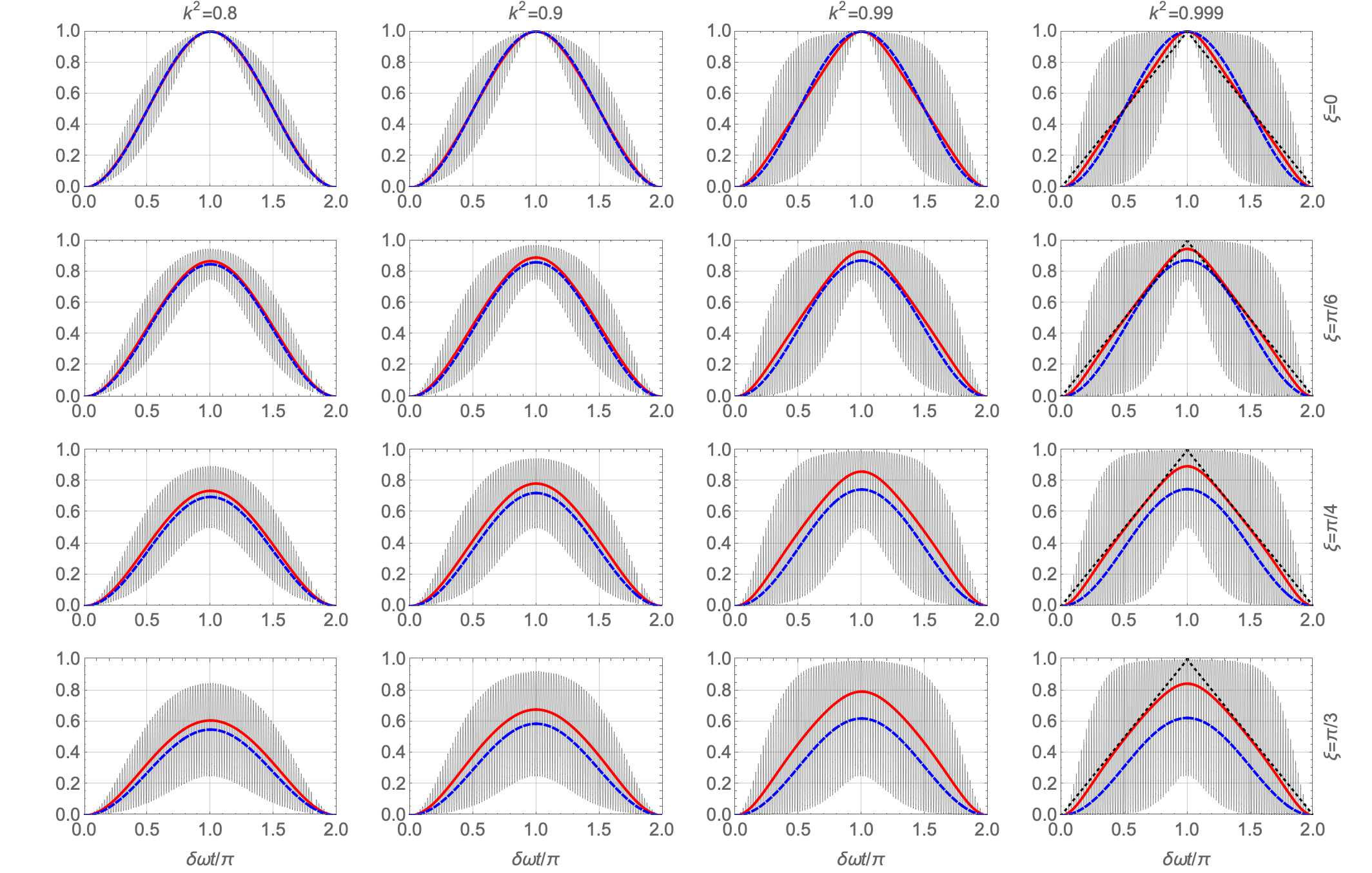
Figure 4: The graph of ℱ​(ω​t,Ύ​ω​t)â„±đœ”đ‘Ąđ›żđœ”đ‘Ą\mathcal{F}(\omega t,\delta\omega\,t) when 2​ω/Ύ​ω=(ω1+ω2)/(ω1−ω2)=1002𝜔𝛿𝜔subscript𝜔1subscript𝜔2subscript𝜔1subscript𝜔21002\omega/\delta\omega=(\omega_{1}+\omega_{2})/(\omega_{1}-\omega_{2})=100, for the cases k2=0.8superscript𝑘20.8k^{2}=0.8, 0.90.90.9, 0.990.990.99, 0.9990.9990.999 and Ο=0𝜉0\xi=0, π6𝜋6\frac{\pi}{6}, π4𝜋4\frac{\pi}{4}, π3𝜋3\frac{\pi}{3}. Graphs for the same value of k2superscript𝑘2k^{2} are arranged in columns while those for the same value of ÎŸđœ‰\xi are arranged in rows. Red: graph of ℱ¯​(Ύ​ω​t)ÂŻâ„±đ›żđœ”đ‘Ą\overline{\mathcal{F}}(\delta\omega\,t) which averages over the rapid oscillations of ℱ​(ω​t,Ύ​ω​t)â„±đœ”đ‘Ąđ›żđœ”đ‘Ą\mathcal{F}(\omega t,\delta\omega\,t). Blue dashed: graph of Eq. (109). Note that the red graph is well approximated by the blue, especially for small ÎŸđœ‰\xi, until k2superscript𝑘2k^{2} closely approaches 1. In the limit k2→1→superscript𝑘21k^{2}\to 1, the locally averaged graph (red line) converges to the saw-tooth function indicated with the black dotted line on the graphs in the rightmost column (k2=0.999superscript𝑘20.999k^{2}=0.999).

For k≠0𝑘0k\neq 0 the dependence on ω​t𝜔𝑡\omega t remains. However, when E≫mimuch-greater-than𝐾subscript𝑚𝑖E\gg m_{i} we have ω≫Ύ​ωmuch-greater-than𝜔𝛿𝜔\omega\gg\delta\omega, and in the expression for ℱ​(ω​t,Ύ​ω​t)â„±đœ”đ‘Ąđ›żđœ”đ‘Ą\mathcal{F}(\omega t,\delta\omega\,t) given in Eq. (101), Sn2​(ω​t,k)superscriptSn2𝜔𝑡𝑘\mathrm{Sn}^{2}(\omega t,k) will oscillate very rapidly compared to Sn2​(Ύ​ω​t/2,k)superscriptSn2𝛿𝜔𝑡2𝑘\mathrm{Sn}^{2}(\delta\omega\,t/2,k). We expect such rapid oscillations to be unobservable, and that ℱ​(ω​t,Δ)â„±đœ”đ‘ĄÎ”\mathcal{F}(\omega t,\Delta) can be replaced by the function ℱ¯​(Δ)¯ℱΔ\overline{\mathcal{F}}(\Delta) where

ℱ¯​(y)=12â€‹Ï€â€‹âˆ«âˆ’Ï€Ï€đ‘‘x​ℱ​(x,y).ÂŻâ„±đ‘Š12𝜋superscriptsubscript𝜋𝜋differential-dđ‘„â„±đ‘„đ‘Š\overline{\mathcal{F}}(y)\;=\;\dfrac{1}{2\pi}\int_{-\pi}^{\pi}dx\,\mathcal{F}(x,y)\;. (107)

We demonstrate this in FIG. 4 which shows graphs of ℱ​(ω​t,Ύ​ω​t)â„±đœ”đ‘Ąđ›żđœ”đ‘Ą\mathcal{F}(\omega t,\delta\omega\,t) for several choices of k2superscript𝑘2k^{2} and ÎŸđœ‰\xi for the case

2​ωΎ​ω=ω1+ω2ω1−ω2= 100.2𝜔𝛿𝜔subscript𝜔1subscript𝜔2subscript𝜔1subscript𝜔2100\dfrac{2\omega}{\delta\omega}\;=\;\dfrac{\omega_{1}+\omega_{2}}{\omega_{1}-\omega_{2}}\;=\;100\;. (108)

We can see that ℱ​(ω​t,Ύ​ω​t)â„±đœ”đ‘Ąđ›żđœ”đ‘Ą\mathcal{F}(\omega t,\delta\omega\,t) oscillates rapidly around the more slowly varying function ℱ¯​(Ύ​ω​t)ÂŻâ„±đ›żđœ”đ‘Ą\overline{\mathcal{F}}(\delta\omega\,t) shown in red. Using the expansion of the Jacobi elliptic functions in k2superscript𝑘2k^{2} given in Appendix B, we can show that ℱ¯​(Ύ​ω​t)ÂŻâ„±đ›żđœ”đ‘Ą\overline{\mathcal{F}}(\delta\omega\,t) can be approximated by

ℱ¯​(Ύ​ω​t)ÂŻâ„±đ›żđœ”đ‘Ą\displaystyle\overline{\mathcal{F}}(\delta\omega\,t) =\displaystyle= (cΟ2+sΟ2​k22)​sin2⁡Δ2+O​(k4).superscriptsubscript𝑐𝜉2superscriptsubscript𝑠𝜉2superscript𝑘22superscript2Δ2𝑂superscript𝑘4\displaystyle\bigg{(}c_{\xi}^{2}+s_{\xi}^{2}\dfrac{k^{2}}{2}\bigg{)}\sin^{2}\dfrac{\Delta}{2}+O(k^{4})\;. (109)

This graph is also shown on FIG. 4 in dashed blue, and we see that this approximation breaks down only when k2superscript𝑘2k^{2} is very close to 1.

IV Bound from Atmospheric Neutrinos
Refer to caption
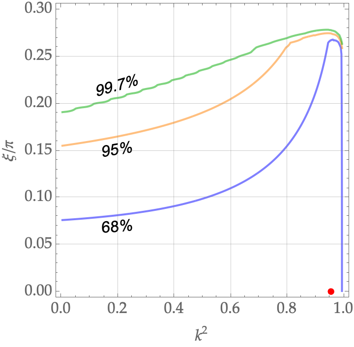
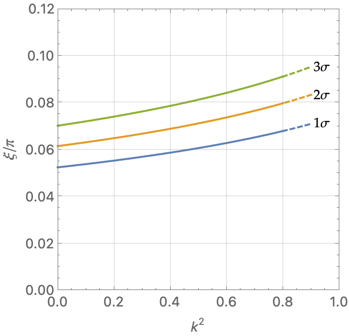
Figure 5: k2superscript𝑘2k^{2}-ÎŸđœ‰\xi contour plot showing the 1​σ1𝜎1\sigma (blue), 2​σ2𝜎2\sigma (orange), and 3​σ3𝜎3\sigma (green) bounds from atmospheric neutrino data and Eq. (109), assuming Normal Ordering. ÎŸđœ‰\xi is in units of Ï€đœ‹\pi. The contours are not continued to the right of k2=0.9superscript𝑘20.9k^{2}=0.9 where the validity of Eq. (109) becomes problematic as k2→1→superscript𝑘21k^{2}\to 1. We expect a more thorough analysis to lead to the contours dropping down to the k2superscript𝑘2k^{2} axis near k2=1superscript𝑘21k^{2}=1.

The expression we obtained in Eq. (109) is just the usual neutrino oscillation formula scaled by the constant (cΟ2+sΟ2​k22)superscriptsubscript𝑐𝜉2superscriptsubscript𝑠𝜉2superscript𝑘22\left(c_{\xi}^{2}+s_{\xi}^{2}\frac{k^{2}}{2}\right). If we consider atmospheric neutrino oscillations, this factor cannot always be absorbed into sin2⁥(2​ξ23)≀1superscript22subscript𝜃231\sin^{2}{(2\theta_{23})}\leq 1, so we can interpret the bounds on the quantity sin2⁥(2​ξ23)superscript22subscript𝜃23\sin^{2}{(2\theta_{23})} as bounds on (cΟ2+sΟ2​k22)​sin2⁥(2​ξ23)superscriptsubscript𝑐𝜉2superscriptsubscript𝑠𝜉2superscript𝑘22superscript22subscript𝜃23\left(c_{\xi}^{2}+s_{\xi}^{2}\frac{k^{2}}{2}\right)\;\sin^{2}{(2\theta_{23})}. According to TABLE III of Ref. [38], the current bounds on sin2⁥Ξ23superscript2subscript𝜃23\sin^{2}\theta_{23} are

sin2⁥Ξ23superscript2subscript𝜃23\displaystyle\sin^{2}\theta_{23} =\displaystyle= 0.566−0.022+0.016(Normal Ordering, 1​σ)\displaystyle 0.566{}^{+0.016}_{-0.022}\qquad\;\;\;\mbox{(Normal Ordering, $1\sigma$)}\vphantom{\Big{|}} (110)
=\displaystyle= 0.505−0.596(NO, 2​σ),0.5050.596(NO, 2σ)\displaystyle 0.505-0.596\qquad\mbox{(NO, $2\sigma$)}\;,\vphantom{\Big{|}} (111)
=\displaystyle= 0.441−0.609(NO, 3​σ),0.4410.609(NO, 3σ)\displaystyle 0.441-0.609\qquad\mbox{(NO, $3\sigma$)}\;,\vphantom{\Big{|}} (112)
=\displaystyle= 0.566−0.023+0.018(Inverted Ordering, 1​σ)\displaystyle 0.566{}^{+0.018}_{-0.023}\qquad\;\;\;\mbox{(Inverted Ordering, $1\sigma$)}\vphantom{\Big{|}} (113)
=\displaystyle= 0.514−0.597(IO, 2​σ),0.5140.597(IO, 2σ)\displaystyle 0.514-0.597\qquad\mbox{(IO, $2\sigma$)}\;,\vphantom{\Big{|}} (114)
=\displaystyle= 0.446−0.609(IO, 3​σ),0.4460.609(IO, 3σ)\displaystyle 0.446-0.609\qquad\mbox{(IO, $3\sigma$)}\;,\vphantom{\Big{|}} (115)

leading to the bounds on sin2⁡2​ξ23=4​sin2⁡ξ23​(1−sin2⁡ξ23)superscript22subscript𝜃234superscript2subscript𝜃231superscript2subscript𝜃23\sin^{2}2\theta_{23}=4\sin^{2}\theta_{23}(1-\sin^{2}\theta_{23}) given by

sin2⁥2​ξ23superscript22subscript𝜃23\displaystyle\sin^{2}2\theta_{23} =\displaystyle= 0.973−0.992(NO, 1​σ)0.9730.992(NO, 1σ)\displaystyle 0.973-0.992\qquad\mbox{(NO, $1\sigma$)}\vphantom{\big{|}} (116)
=\displaystyle= 0.963−1.000(NO, 2​σ)0.9631.000(NO, 2σ)\displaystyle 0.963-1.000\qquad\mbox{(NO, $2\sigma$)}\vphantom{\big{|}} (117)
=\displaystyle= 0.952−1.000(NO, 3​σ)0.9521.000(NO, 3σ)\displaystyle 0.952-1.000\qquad\mbox{(NO, $3\sigma$)}\vphantom{\big{|}} (118)
=\displaystyle= 0.972−0.993(IO, 1​σ)0.9720.993(IO, 1σ)\displaystyle 0.972-0.993\qquad\mbox{(IO, $1\sigma$)}\vphantom{\big{|}} (119)
=\displaystyle= 0.962−0.999(IO, 2​σ)0.9620.999(IO, 2σ)\displaystyle 0.962-0.999\qquad\mbox{(IO, $2\sigma$)}\vphantom{\big{|}} (120)
=\displaystyle= 0.952−1.000(IO, 3​σ)0.9521.000(IO, 3σ)\displaystyle 0.952-1.000\qquad\mbox{(IO, $3\sigma$)}\vphantom{\big{|}} (121)

So the bounds for both the NO and IO cases are more or less the same. The NO numbers translate to

sΟ2​(1−k22)superscriptsubscript𝑠𝜉21superscript𝑘22\displaystyle s_{\xi}^{2}\left(1-\dfrac{k^{2}}{2}\right) <\displaystyle< 1−0.973= 0.027(1​σ),10.9730.0271𝜎\displaystyle 1-0.973\;=\;0.027\qquad(1\sigma)\;, (122)
<\displaystyle< 1−0.963= 0.037(2​σ),10.9630.0372𝜎\displaystyle 1-0.963\;=\;0.037\qquad(2\sigma)\;, (123)
<\displaystyle< 1−0.952= 0.048(3​σ).10.9520.0483𝜎\displaystyle 1-0.952\;=\;0.048\qquad(3\sigma)\;.\vphantom{\bigg{|}} (124)

For the k=0𝑘0k=0 case, this translates to

Οπ< 0.053​(1​σ),0.062​(2​σ),0.070​(3​σ).𝜉𝜋0.0531𝜎0.0622𝜎0.0703𝜎\dfrac{\xi}{\pi}\;<\;0.053\;\;(1\sigma)\;,\quad 0.062\;\;(2\sigma)\;,\quad 0.070\;\;(3\sigma)\;. (125)

For non-zero k𝑘k, see FIG. 5 for the likelihood contours on the k2superscript𝑘2k^{2}-ÎŸđœ‰\xi plane. In FIG. 5, the contours are not extended all the way to k2=1superscript𝑘21k^{2}=1 since Eq. (109) is unreliable in that region. They can be expected to turn downward and reach the k2superscript𝑘2k^{2} axis before reaching k2=1superscript𝑘21k^{2}=1 since the oscillation function ℱ¯​(Δ)¯ℱΔ\overline{\mathcal{F}}(\Delta) will start to deviate from the sinusoidal as k2→1→superscript𝑘21k^{2}\to 1 as shown in FIG. 4. A complete oscillation analysis would be necessary to work out the bounds on ÎŸđœ‰\xi and k2superscript𝑘2k^{2} in this region. We do not perform this analysis in this paper due to reasons that are given in the discussion session. Instead, we look at B0superscriptđ”0B^{0}-B0ÂŻÂŻsuperscriptđ”0\overline{B^{0}} oscillation next.

V B0superscriptđ”0B^{0}-B0ÂŻÂŻsuperscriptđ”0\overline{B^{0}} Oscillation

Another oscillation phenomenon that has been extensively studied in experiments is that of time-dependent CP asymmetry in meson-antimeson oscillations [39, 40] for which a wealth of data exist from Belle and BABAR. In the following, we place bounds on k𝑘k and ÎŸđœ‰\xi utilizing the B0superscriptđ”0B^{0}-B0ÂŻÂŻsuperscriptđ”0\overline{B^{0}} oscillation data from Belle.

V.1 Canonical QM Case

Consider the oscillation of B0superscriptđ”0B^{0} into B0ÂŻÂŻsuperscriptđ”0\overline{B^{0}} and vice versa before they decay into a common physical state f𝑓f. Recall that in the usual canonical QM formulation, the CP eigenstates are (|B0⟩±|B0ÂŻâŸ©)/2plus-or-minusketsuperscriptđ”0ketÂŻsuperscriptđ”02(\big{|}B^{0}\big{\rangle}\pm\big{|}\overline{B^{0}}\big{\rangle})/\sqrt{2}, whereas the mass eigenstates are [41]

|BL0⟩ketsuperscriptsubscriptđ”đż0\displaystyle\big{|}B_{L}^{0}\big{\rangle} =\displaystyle= p​|B0⟩+q​|B0ÂŻâŸ©,𝑝ketsuperscriptđ”0𝑞ketÂŻsuperscriptđ”0\displaystyle p\big{|}B^{0}\big{\rangle}+q\big{|}\overline{B^{0}}\big{\rangle}\;,\vphantom{\Big{|}} (126)
|BH0⟩ketsuperscriptsubscriptđ”đ»0\displaystyle\big{|}B_{H}^{0}\big{\rangle} =\displaystyle= p​|B0⟩−q​|B0ÂŻâŸ©,𝑝ketsuperscriptđ”0𝑞ketÂŻsuperscriptđ”0\displaystyle p\big{|}B^{0}\big{\rangle}-q\big{|}\overline{B^{0}}\big{\rangle}\;,\vphantom{\Big{|}} (127)

where |p|=|q|=1/2𝑝𝑞12|p|=|q|=1/\sqrt{2}, and p𝑝p and q𝑞q have opposite phase:

p=12​x→​(ϕ),q=12​x→​(−ϕ).formulae-sequence𝑝12â†’đ‘„italic-Ï•đ‘ž12â†’đ‘„italic-ϕp\;=\;\dfrac{1}{\sqrt{2}}\,\vec{x}(\phi)\;,\qquad q\;=\;\dfrac{1}{\sqrt{2}}\,\vec{x}(-\phi)\;. (128)

To leading order in the Standard Model, the CP violating phase ϕitalic-ϕ\phi is given by [41]

x→​(2​ϕ)=pq=Vt​b​Vt​d∗Vt​b∗​Vt​d.â†’đ‘„2italic-Ï•đ‘đ‘žsuperscriptsubscript𝑉𝑡𝑏absentsubscriptsuperscript𝑉𝑡𝑑subscriptsuperscript𝑉𝑡𝑏superscriptsubscript𝑉𝑡𝑑absent\vec{x}(2\phi)\;=\;\dfrac{p}{q}\;=\;\frac{V_{tb}^{\vphantom{*}}V^{*}_{td}}{V^{*}_{tb}V_{td}^{\vphantom{*}}}\;. (129)

To facilitate the application of our Nambu extension later, we work in the mass eigenstate basis, in which the B0superscriptđ”0B^{0} and B0ÂŻÂŻsuperscriptđ”0\overline{B^{0}} states are expressed as superpositions of the mass eigenstates BL0superscriptsubscriptđ”đż0B_{L}^{0} and BH0superscriptsubscriptđ”đ»0B_{H}^{0} :

|B0⟩ketsuperscriptđ”0\displaystyle\big{|}B^{0}\big{\rangle} =\displaystyle= q​|BL0⟩+q​|BH0⟩,𝑞ketsubscriptsuperscriptđ”0𝐿𝑞ketsubscriptsuperscriptđ”0đ»\displaystyle q\big{|}B^{0}_{L}\big{\rangle}+q\big{|}B^{0}_{H}\big{\rangle}\;,\vphantom{\Big{|}} (130)
|B0ÂŻâŸ©ketÂŻsuperscriptđ”0\displaystyle\big{|}\overline{B^{0}}\big{\rangle} =\displaystyle= p​|BL0⟩−p​|BH0⟩.𝑝ketsubscriptsuperscriptđ”0𝐿𝑝ketsubscriptsuperscriptđ”0đ»\displaystyle p\big{|}B^{0}_{L}\big{\rangle}-p\big{|}B^{0}_{H}\big{\rangle}\;.\vphantom{\Big{|}} (131)

In the rest frame of the particle, the mass eigenstates |BL0⟩ketsubscriptsuperscriptđ”0𝐿\big{|}B^{0}_{L}\big{\rangle} and |BH0⟩ketsubscriptsuperscriptđ”0đ»\big{|}B^{0}_{H}\big{\rangle} evolve as

|BL0​(t)⟩=e−(ΓL/2)​t​x→​(−mL​t)​|BL0​(0)⟩,|BH0​(t)⟩=e−(ΓH/2)​t​x→​(−mH​t)​|BH0​(0)⟩,formulae-sequenceketsuperscriptsubscriptđ”đż0𝑡superscript𝑒subscriptΓ𝐿2đ‘Ąâ†’đ‘„subscript𝑚𝐿𝑡ketsuperscriptsubscriptđ”đż00ketsuperscriptsubscriptđ”đ»0𝑡superscript𝑒subscriptÎ“đ»2đ‘Ąâ†’đ‘„subscriptđ‘šđ»đ‘Ąketsuperscriptsubscriptđ”đ»00\big{|}B_{L}^{0}(t)\big{\rangle}\,=\,e^{-(\Gamma_{L}/2)t}\,\vec{x}(-m_{L}t)\big{|}B_{L}^{0}(0)\big{\rangle}\;,\qquad\big{|}B_{H}^{0}(t)\big{\rangle}\,=\,e^{-(\Gamma_{H}/2)t}\,\vec{x}(-m_{H}t)\big{|}B_{H}^{0}(0)\big{\rangle}\;, (132)

so the B0superscriptđ”0B^{0} superposition evolves as

|B0​(0)⟩ketsuperscriptđ”00\displaystyle\big{|}B^{0}(0)\big{\rangle} =\displaystyle= 12​x→​(−ϕ)​|BL0​(0)⟩+12​x→​(−ϕ)​|BH0​(0)⟩12â†’đ‘„italic-ϕketsubscriptsuperscriptđ”0𝐿012â†’đ‘„italic-ϕketsubscriptsuperscriptđ”0đ»0\displaystyle\dfrac{1}{\sqrt{2}}\vec{x}(-\phi)\big{|}B^{0}_{L}(0)\big{\rangle}+\dfrac{1}{\sqrt{2}}\vec{x}(-\phi)\big{|}B^{0}_{H}(0)\big{\rangle} (133)
↓↓\displaystyle\downarrow (134)
|B0​(t)⟩ketsuperscriptđ”0𝑡\displaystyle\big{|}B^{0}(t)\big{\rangle} =\displaystyle= 12​e−(ΓL/2)​t​x→​(−ϕ)​|BL0​(t)⟩+12​e−(ΓH/2)​t​x→​(−ϕ)​|BH0​(t)⟩12superscript𝑒subscriptΓ𝐿2đ‘Ąâ†’đ‘„italic-ϕketsubscriptsuperscriptđ”0𝐿𝑡12superscript𝑒subscriptÎ“đ»2đ‘Ąâ†’đ‘„italic-ϕketsubscriptsuperscriptđ”0đ»đ‘Ą\displaystyle\dfrac{1}{\sqrt{2}}\,e^{-(\Gamma_{L}/2)t}\,\vec{x}(-\phi)\big{|}B^{0}_{L}(t)\big{\rangle}+\dfrac{1}{\sqrt{2}}\,e^{-(\Gamma_{H}/2)t}\,\vec{x}(-\phi)\big{|}B^{0}_{H}(t)\big{\rangle}\vphantom{\Bigg{|}} (135)
=\displaystyle= 12​e−(ΓL/2)​t​x→​(−ϕ−mL​t)​|BL0​(0)⟩+12​e−(ΓH/2)​t​x→​(−ϕ−mH​t)​|BH0​(0)⟩.12superscript𝑒subscriptΓ𝐿2đ‘Ąâ†’đ‘„italic-ϕsubscript𝑚𝐿𝑡ketsubscriptsuperscriptđ”0𝐿012superscript𝑒subscriptÎ“đ»2đ‘Ąâ†’đ‘„italic-ϕsubscriptđ‘šđ»đ‘Ąketsubscriptsuperscriptđ”0đ»0\displaystyle\dfrac{1}{\sqrt{2}}\,e^{-(\Gamma_{L}/2)t}\,\vec{x}(-\phi-m_{L}t)\big{|}B^{0}_{L}(0)\big{\rangle}+\dfrac{1}{\sqrt{2}}\,e^{-(\Gamma_{H}/2)t}\,\vec{x}(-\phi-m_{H}t)\big{|}B^{0}_{H}(0)\big{\rangle}\;. (136)

We assume that ΓL=ΓHsubscriptΓ𝐿subscriptÎ“đ»\Gamma_{L}=\Gamma_{H}, and drop the common decay factor from this point on. Then, we find

g​(B0​(0),B0​(t))𝑔superscriptđ”00superscriptđ”0𝑡\displaystyle g(B^{0}(0),B^{0}(t)) =\displaystyle= 12​x→​(−ϕ)⋅x→​(−ϕ−mL​t)+12​x→​(−ϕ)⋅x→​(−ϕ−mH​t)⋅12â†’đ‘„italic-Ï•â†’đ‘„italic-ϕsubscript𝑚𝐿𝑡⋅12â†’đ‘„italic-Ï•â†’đ‘„italic-ϕsubscriptđ‘šđ»đ‘Ą\displaystyle\dfrac{1}{2}\vec{x}(-\phi)\cdot\vec{x}(-\phi-m_{L}t)+\dfrac{1}{2}\vec{x}(-\phi)\cdot\vec{x}(-\phi-m_{H}t)\vphantom{\Bigg{|}} (137)
=\displaystyle= 12​[cos⁥(mL​t)+cos⁥(mH​t)]12delimited-[]subscript𝑚𝐿𝑡subscriptđ‘šđ»đ‘Ą\displaystyle\dfrac{1}{2}\Big{[}\cos(m_{L}t)+\cos(m_{H}t)\Big{]}\vphantom{\Bigg{|}} (138)
=\displaystyle= cos⁡(m​t)​cos⁡(Δ​m​t2),𝑚𝑡Δ𝑚𝑡2\displaystyle\cos(mt)\cos\bigg{(}\dfrac{\Delta m\,t}{2}\bigg{)}\;,\vphantom{\bigg{|}} (139)
Δ​(B0​(0),B0​(t))𝜀superscriptđ”00superscriptđ”0𝑡\displaystyle\varepsilon(B^{0}(0),B^{0}(t)) =\displaystyle= 12​x→​(−ϕ)×x→​(−ϕ−mL​t)+12​x→​(−ϕ)×x→​(−ϕ−mH​t)12â†’đ‘„italic-Ï•â†’đ‘„italic-ϕsubscript𝑚𝐿𝑡12â†’đ‘„italic-Ï•â†’đ‘„italic-ϕsubscriptđ‘šđ»đ‘Ą\displaystyle\dfrac{1}{2}\vec{x}(-\phi)\times\vec{x}(-\phi-m_{L}t)+\dfrac{1}{2}\vec{x}(-\phi)\times\vec{x}(-\phi-m_{H}t)\vphantom{\Bigg{|}} (140)
=\displaystyle= −12​[sin⁥(mL​t)+sin⁥(mH​t)]12delimited-[]subscript𝑚𝐿𝑡subscriptđ‘šđ»đ‘Ą\displaystyle-\dfrac{1}{2}\Big{[}\sin(m_{L}t)+\sin(m_{H}t)\Big{]}\vphantom{\Bigg{|}} (141)
=\displaystyle= −sin⁡(m​t)​cos⁡(Δ​m​t2),𝑚𝑡Δ𝑚𝑡2\displaystyle-\sin(mt)\cos\bigg{(}\dfrac{\Delta m\,t}{2}\bigg{)}\;,\vphantom{\bigg{|}} (142)
g​(B0¯​(0),B0​(t))𝑔¯superscriptđ”00superscriptđ”0𝑡\displaystyle g(\overline{B^{0}}(0),B^{0}(t)) =\displaystyle= 12​x→​(ϕ)⋅x→​(−ϕ−mL​t)−12​x→​(ϕ)⋅x→​(−ϕ−mH​t)⋅12â†’đ‘„italic-Ï•â†’đ‘„italic-ϕsubscript𝑚𝐿𝑡⋅12â†’đ‘„italic-Ï•â†’đ‘„italic-ϕsubscriptđ‘šđ»đ‘Ą\displaystyle\dfrac{1}{2}\vec{x}(\phi)\cdot\vec{x}(-\phi-m_{L}t)-\dfrac{1}{2}\vec{x}(\phi)\cdot\vec{x}(-\phi-m_{H}t)\vphantom{\Bigg{|}} (143)
=\displaystyle= 12​[cos⁥(2​ϕ+mL​t)−cos⁥(2​ϕ+mH​t)]12delimited-[]2italic-ϕsubscript𝑚𝐿𝑡2italic-ϕsubscriptđ‘šđ»đ‘Ą\displaystyle\dfrac{1}{2}\Big{[}\cos(2\phi+m_{L}t)-\cos(2\phi+m_{H}t)\Big{]}\vphantom{\Bigg{|}} (144)
=\displaystyle= sin⁥(2​ϕ+m​t)​sin⁥(Δ​m​t2),2italic-Ï•đ‘šđ‘ĄÎ”đ‘šđ‘Ą2\displaystyle\sin(2\phi+mt)\sin\bigg{(}\dfrac{\Delta m\,t}{2}\bigg{)}\;,\vphantom{\bigg{|}} (145)
Δ​(B0¯​(0),B0​(t))𝜀¯superscriptđ”00superscriptđ”0𝑡\displaystyle\varepsilon(\overline{B^{0}}(0),B^{0}(t)) =\displaystyle= 12​x→​(ϕ)×x→​(−ϕ−mL​t)−12​x→​(ϕ)×x→​(−ϕ−mH​t)12â†’đ‘„italic-Ï•â†’đ‘„italic-ϕsubscript𝑚𝐿𝑡12â†’đ‘„italic-Ï•â†’đ‘„italic-ϕsubscriptđ‘šđ»đ‘Ą\displaystyle\dfrac{1}{2}\vec{x}(\phi)\times\vec{x}(-\phi-m_{L}t)-\dfrac{1}{2}\vec{x}(\phi)\times\vec{x}(-\phi-m_{H}t)\vphantom{\Bigg{|}} (146)
=\displaystyle= −12​[sin⁥(2​ϕ+mL​t)−sin⁥(2​ϕ+mH​t)]12delimited-[]2italic-ϕsubscript𝑚𝐿𝑡2italic-ϕsubscriptđ‘šđ»đ‘Ą\displaystyle-\dfrac{1}{2}\Big{[}\sin(2\phi+m_{L}t)-\sin(2\phi+m_{H}t)\Big{]}\vphantom{\Bigg{|}} (147)
=\displaystyle= cos⁥(2​ϕ+m​t)​sin⁥(Δ​m​t2),2italic-Ï•đ‘šđ‘ĄÎ”đ‘šđ‘Ą2\displaystyle\cos(2\phi+mt)\sin\bigg{(}\dfrac{\Delta m\,t}{2}\bigg{)}\;,\vphantom{\bigg{|}} (148)

where

m=mL+mH2,Δ​m=mH−mL.formulae-sequence𝑚subscript𝑚𝐿subscriptđ‘šđ»2Δ𝑚subscriptđ‘šđ»subscript𝑚𝐿m\,=\,\dfrac{m_{L}+m_{H}}{2}\;,\qquad\Delta m\,=\,m_{H}-m_{L}\;. (149)

The survival and transition probabilities evolve with time as

P​(B0→B0)𝑃→superscriptđ”0superscriptđ”0\displaystyle P(B^{0}\to B^{0}) =\displaystyle= g​(B0​(0),B0​(t))2+Δ​(B0​(0),B0​(t))2=cos2⁥(Δ​m​t2),𝑔superscriptsuperscriptđ”00superscriptđ”0𝑡2𝜀superscriptsuperscriptđ”00superscriptđ”0𝑡2superscript2Δ𝑚𝑡2\displaystyle g(B^{0}(0),B^{0}(t))^{2}+\varepsilon(B^{0}(0),B^{0}(t))^{2}\,=\,\cos^{2}\left(\dfrac{\Delta m\,t}{2}\right)\;,\vphantom{\Bigg{|}} (150)
P​(B0→B0ÂŻ)𝑃→superscriptđ”0ÂŻsuperscriptđ”0\displaystyle P(B^{0}\to\overline{B^{0}}) =\displaystyle= g​(B0¯​(0),B0​(t))2+Δ​(B0¯​(0),B0​(t))2=sin2⁥(Δ​m​t2),𝑔superscriptÂŻsuperscriptđ”00superscriptđ”0𝑡2𝜀superscriptÂŻsuperscriptđ”00superscriptđ”0𝑡2superscript2Δ𝑚𝑡2\displaystyle g(\overline{B^{0}}(0),B^{0}(t))^{2}+\varepsilon(\overline{B^{0}}(0),B^{0}(t))^{2}\,=\,\sin^{2}\left(\dfrac{\Delta m\,t}{2}\right)\;,\vphantom{\Bigg{|}} (151)

with similar relations for P​(B0¯→B0)𝑃→¯superscriptđ”0superscriptđ”0P(\overline{B^{0}}\to B^{0}) and P​(B0¯→B0ÂŻ)𝑃→¯superscriptđ”0ÂŻsuperscriptđ”0P(\overline{B^{0}}\to\overline{B^{0}}).

Consider the asymmetry

A​(t)=|⟹f|B0¯​(t)⟩|2−|⟹f|B0​(t)⟩|2|⟹f|B0¯​(t)⟩|2+|⟹f|B0​(t)⟩|2,𝐮𝑡superscriptinner-product𝑓¯superscriptđ”0𝑡2superscriptinner-product𝑓superscriptđ”0𝑡2superscriptinner-product𝑓¯superscriptđ”0𝑡2superscriptinner-product𝑓superscriptđ”0𝑡2A(t)\;=\;\dfrac{|\langle f|\overline{B^{0}}(t)\rangle|^{2}-|\langle f|B^{0}(t)\rangle|^{2}}{|\langle f|\overline{B^{0}}(t)\rangle|^{2}+|\langle f|B^{0}(t)\rangle|^{2}}\;, (152)

where ⟹f|B0​(t)⟩inner-product𝑓superscriptđ”0𝑡\langle f|B^{0}(t)\rangle and ⟹f|BÂŻ0​(t)⟩inner-product𝑓superscriptÂŻđ”0𝑡\langle f|\overline{B}^{0}(t)\rangle are the amplitudes of the states |B0​(t)⟩ketsuperscriptđ”0𝑡\big{|}B^{0}(t)\big{\rangle} and |BÂŻ0​(t)⟩ketsuperscriptÂŻđ”0𝑡\big{|}\overline{B}^{0}(t)\big{\rangle} decaying into f𝑓f respectively. Let

⟹f|BL0​(0)⟩=AL​x→​(−λ),⟹f|BH0​(0)⟩=AH​x→​(−η),formulae-sequenceinner-product𝑓subscriptsuperscriptđ”0𝐿0subscriptđŽđżâ†’đ‘„đœ†inner-product𝑓subscriptsuperscriptđ”0đ»0subscriptđŽđ»â†’đ‘„đœ‚\langle f|B^{0}_{L}(0)\rangle\,=\,A_{L}\,\vec{x}(-\lambda)\;,\qquad\langle f|B^{0}_{H}(0)\rangle\,=\,A_{H}\,\vec{x}(-\eta)\;, (153)

that is

|f⟩=|BL0​(0)⟩​⟚BL0​(0)|f⟩⏟AL​x→​(λ)+|BH0​(0)⟩​⟚BH0​(0)|f⟩⏟AH​x→​(η)+⋯.ket𝑓ketsubscriptsuperscriptđ”0𝐿0subscript⏟inner-productsubscriptsuperscriptđ”0𝐿0𝑓subscriptđŽđżâ†’đ‘„đœ†ketsubscriptsuperscriptđ”0đ»0subscript⏟inner-productsubscriptsuperscriptđ”0đ»0𝑓subscriptđŽđ»â†’đ‘„đœ‚â‹Ż\big{|}f\big{\rangle}\;=\;\big{|}B^{0}_{L}(0)\big{\rangle}\underbrace{\langle B^{0}_{L}(0)|f\rangle}_{\displaystyle A_{L}\vec{x}(\lambda)}+\big{|}B^{0}_{H}(0)\big{\rangle}\underbrace{\langle B^{0}_{H}(0)|f\rangle}_{\displaystyle A_{H}\vec{x}(\eta)}+\cdots\;. (154)

Then,

g​(f,B0​(t))𝑔𝑓superscriptđ”0𝑡\displaystyle g(f,B^{0}(t)) =\displaystyle= AL2​x→​(λ)⋅x→​(−ϕ−mL​t)+AH2​x→​(η)⋅x→​(−ϕ−mH​t)⋅subscript𝐮𝐿2â†’đ‘„đœ†â†’đ‘„italic-ϕsubscript𝑚𝐿𝑡⋅subscriptđŽđ»2â†’đ‘„đœ‚â†’đ‘„italic-ϕsubscriptđ‘šđ»đ‘Ą\displaystyle\dfrac{A_{L}}{\sqrt{2}}\,\vec{x}(\lambda)\cdot\vec{x}(-\phi-m_{L}t)+\dfrac{A_{H}}{\sqrt{2}}\,\vec{x}(\eta)\cdot\vec{x}(-\phi-m_{H}t)\vphantom{\Bigg{|}} (155)
=\displaystyle= AL2​cos⁥(λ+ϕ+mL​t)+AH2​cos⁥(η+ϕ+mH​t),subscript𝐮𝐿2𝜆italic-ϕsubscript𝑚𝐿𝑡subscriptđŽđ»2𝜂italic-ϕsubscriptđ‘šđ»đ‘Ą\displaystyle\dfrac{A_{L}}{\sqrt{2}}\cos(\lambda+\phi+m_{L}t)+\dfrac{A_{H}}{\sqrt{2}}\cos(\eta+\phi+m_{H}t)\;,\vphantom{\Bigg{|}} (156)
Δ​(f,B0​(t))𝜀𝑓superscriptđ”0𝑡\displaystyle\varepsilon(f,B^{0}(t)) =\displaystyle= AL2​x→​(λ)×x→​(−ϕ−mL​t)+AH2​x→​(η)×x→​(−ϕ−mH​t)subscript𝐮𝐿2â†’đ‘„đœ†â†’đ‘„italic-ϕsubscript𝑚𝐿𝑡subscriptđŽđ»2â†’đ‘„đœ‚â†’đ‘„italic-ϕsubscriptđ‘šđ»đ‘Ą\displaystyle\dfrac{A_{L}}{\sqrt{2}}\,\vec{x}(\lambda)\times\vec{x}(-\phi-m_{L}t)+\dfrac{A_{H}}{\sqrt{2}}\,\vec{x}(\eta)\times\vec{x}(-\phi-m_{H}t)\vphantom{\Bigg{|}} (157)
=\displaystyle= −AL2​sin⁥(λ+ϕ+mL​t)−AH2​sin⁥(η+ϕ+mH​t),subscript𝐮𝐿2𝜆italic-ϕsubscript𝑚𝐿𝑡subscriptđŽđ»2𝜂italic-ϕsubscriptđ‘šđ»đ‘Ą\displaystyle-\dfrac{A_{L}}{\sqrt{2}}\sin(\lambda+\phi+m_{L}t)-\dfrac{A_{H}}{\sqrt{2}}\sin(\eta+\phi+m_{H}t)\;,\vphantom{\Bigg{|}}\vphantom{\Bigg{|}} (158)

and

|⟹f|B0​(t)⟩|2superscriptinner-product𝑓superscriptđ”0𝑡2\displaystyle|\langle f|B^{0}(t)\rangle|^{2} =\displaystyle= g​(f,B0​(t))2+Δ​(f,B0​(t))2𝑔superscript𝑓superscriptđ”0𝑡2𝜀superscript𝑓superscriptđ”0𝑡2\displaystyle g(f,B^{0}(t))^{2}+\varepsilon(f,B^{0}(t))^{2}\vphantom{\bigg{|}} (159)
=\displaystyle= AL22+AH22+AL​AH​{cos⁥(η−λ)​cos⁥(Δ​m​t)−sin⁥(η−λ)​sin⁥(Δ​m​t)}.superscriptsubscript𝐮𝐿22superscriptsubscriptđŽđ»22subscript𝐮𝐿subscriptđŽđ»đœ‚đœ†Î”đ‘šđ‘Ąđœ‚đœ†Î”đ‘šđ‘Ą\displaystyle\dfrac{A_{L}^{2}}{2}+\dfrac{A_{H}^{2}}{2}+A_{L}A_{H}\Big{\{}\cos(\eta-\lambda)\cos(\Delta m\,t)-\sin(\eta-\lambda)\sin(\Delta m\,t)\Big{\}}\;. (160)

Similarly,

|⟹f|B0¯​(t)⟩|2=AL22+AH22−AL​AH​{cos⁥(η−λ)​cos⁥(Δ​m​t)−sin⁥(η−λ)​sin⁥(Δ​m​t)},superscriptinner-product𝑓¯superscriptđ”0𝑡2superscriptsubscript𝐮𝐿22superscriptsubscriptđŽđ»22subscript𝐮𝐿subscriptđŽđ»đœ‚đœ†Î”đ‘šđ‘Ąđœ‚đœ†Î”đ‘šđ‘Ą|\langle f|\overline{B^{0}}(t)\rangle|^{2}\;=\;\dfrac{A_{L}^{2}}{2}+\dfrac{A_{H}^{2}}{2}-A_{L}A_{H}\Big{\{}\cos(\eta-\lambda)\cos(\Delta m\,t)-\sin(\eta-\lambda)\sin(\Delta m\,t)\Big{\}}\;, (161)

and we find

A​(t)𝐮𝑡\displaystyle A(t) =\displaystyle= 2​AL​AHAL2+AH2​sin⁥(η−λ)⏟S​sin⁥(Δ​m​t)−2​AL​AHAL2+AH2​cos⁥(η−λ)⏟C​cos⁥(Δ​m​t)subscript⏟2subscript𝐮𝐿subscriptđŽđ»superscriptsubscript𝐮𝐿2superscriptsubscriptđŽđ»2𝜂𝜆𝑆Δ𝑚𝑡subscript⏟2subscript𝐮𝐿subscriptđŽđ»superscriptsubscript𝐮𝐿2superscriptsubscriptđŽđ»2đœ‚đœ†đ¶Î”đ‘šđ‘Ą\displaystyle\underbrace{\dfrac{2A_{L}A_{H}}{A_{L}^{2}+A_{H}^{2}}\sin(\eta-\lambda)}_{\displaystyle S}\sin(\Delta m\,t)-\underbrace{\dfrac{2A_{L}A_{H}}{A_{L}^{2}+A_{H}^{2}}\cos(\eta-\lambda)}_{\displaystyle C}\cos(\Delta m\,t) (162)
=\displaystyle= S​sin⁥(Δ​m​t)−C​cos⁥(Δ​m​t).đ‘†Î”đ‘šđ‘Ąđ¶Î”đ‘šđ‘Ą\displaystyle S\sin(\Delta m\,t)-C\cos(\Delta m\,t)\vphantom{\bigg{|}}\;. (163)

Note that

S2+C2=(2​AL​AHAL2+AH2)2≀ 1.superscript𝑆2superscriptđ¶2superscript2subscript𝐮𝐿subscriptđŽđ»superscriptsubscript𝐮𝐿2superscriptsubscriptđŽđ»221S^{2}+C^{2}\;=\;\bigg{(}\dfrac{2A_{L}A_{H}}{A_{L}^{2}+A_{H}^{2}}\bigg{)}^{2}\;\leq\;1\;. (164)

It is straightforward to show that the above definitions of S𝑆S and Cđ¶C agree with the usual expressions [41] involving

Afsubscript𝐮𝑓\displaystyle A_{f} =\displaystyle= q​(⟹f|BL⟩+⟹f|BH⟩)=⟹f|B0⟩,and𝑞inner-product𝑓subscriptđ”đżinner-product𝑓subscriptđ”đ»inner-product𝑓superscriptđ”0and\displaystyle q\Big{(}\langle f|B_{L}\rangle+\langle f|B_{H}\rangle\Big{)}\;=\;\langle f|B^{0}\rangle\;,\quad\text{and}\vphantom{\bigg{|}} (165)
AÂŻfsubscript¯𝐮𝑓\displaystyle\bar{A}_{f} =\displaystyle= p​(⟹f|BL⟩−⟚f|BH⟩)=⟹f|BÂŻ0⟩.𝑝inner-product𝑓subscriptđ”đżinner-product𝑓subscriptđ”đ»inner-product𝑓superscriptÂŻđ”0\displaystyle p\Big{(}\langle f|B_{L}\rangle-\langle f|B_{H}\rangle\Big{)}\;=\;\langle f|\overline{B}^{0}\rangle\;.\vphantom{\bigg{|}} (166)

We refrain from this rewriting, however, since the analogs of Afsubscript𝐮𝑓A_{f} and A¯fsubscript¯𝐮𝑓\bar{A}_{f} are ill defined in Nambu QM.

V.2 Nambu QM Extension

Let us now apply the Nambu extension to the above formalism. We assume that the B0superscriptđ”0B^{0} and B0ÂŻÂŻsuperscriptđ”0\overline{B^{0}} states are given by the superpositions

|B0⟩ketsuperscriptđ”0\displaystyle\big{|}B^{0}\big{\rangle} =\displaystyle= Q​|BL0⟩+Q​|BH0⟩,𝑄ketsubscriptsuperscriptđ”0𝐿𝑄ketsubscriptsuperscriptđ”0đ»\displaystyle Q\big{|}B^{0}_{L}\big{\rangle}+Q\big{|}B^{0}_{H}\big{\rangle}\;,\vphantom{\Big{|}} (167)
|B0ÂŻâŸ©ketÂŻsuperscriptđ”0\displaystyle\big{|}\overline{B^{0}}\big{\rangle} =\displaystyle= P​|BL0⟩−P​|BH0⟩,𝑃ketsubscriptsuperscriptđ”0𝐿𝑃ketsubscriptsuperscriptđ”0đ»\displaystyle P\big{|}B^{0}_{L}\big{\rangle}-P\big{|}B^{0}_{H}\big{\rangle}\;,\vphantom{\Big{|}} (168)

where

P=12​Q=12​X→​(ϕ),Q=12​P=12​X→​(−ϕ).formulae-sequence𝑃12𝑄12→𝑋italic-Ï•đ‘„12𝑃12→𝑋italic-ϕP\,=\,\dfrac{1}{2Q}\,=\,\dfrac{1}{\sqrt{2}}\,\vec{X}(\phi)\;,\qquad Q\,=\,\dfrac{1}{2P}\,=\,\dfrac{1}{\sqrt{2}}\,\vec{X}(-\phi)\;. (169)

Here, we suppress the dependence of X→→𝑋\vec{X} on the deformation parameters k𝑘k and ÎŸđœ‰\xi to simplify our notation.

In the rest frame of the particle, the mass eigenstates |BL0⟩ketsubscriptsuperscriptđ”0𝐿\big{|}B^{0}_{L}\big{\rangle} and |BH0⟩ketsubscriptsuperscriptđ”0đ»\big{|}B^{0}_{H}\big{\rangle} evolve as

|BL0​(t)⟩=e−(ΓL/2)​t​X→​(−mL​t)​|BL0​(0)⟩,|BH0​(t)⟩=e−(ΓH/2)​t​X→​(−mH​t)​|BH0​(0)⟩.formulae-sequenceketsuperscriptsubscriptđ”đż0𝑡superscript𝑒subscriptΓ𝐿2𝑡→𝑋subscript𝑚𝐿𝑡ketsuperscriptsubscriptđ”đż00ketsuperscriptsubscriptđ”đ»0𝑡superscript𝑒subscriptÎ“đ»2𝑡→𝑋subscriptđ‘šđ»đ‘Ąketsuperscriptsubscriptđ”đ»00\big{|}B_{L}^{0}(t)\big{\rangle}\,=\,e^{-(\Gamma_{L}/2)t}\,\vec{X}(-m_{L}t)\big{|}B_{L}^{0}(0)\big{\rangle}\;,\qquad\big{|}B_{H}^{0}(t)\big{\rangle}\,=\,e^{-(\Gamma_{H}/2)t}\,\vec{X}(-m_{H}t)\big{|}B_{H}^{0}(0)\big{\rangle}\;. (170)

We assume ΓL=ΓHsubscriptΓ𝐿subscriptÎ“đ»\Gamma_{L}=\Gamma_{H} as in the canonical case and suppress this common decay factor from this point on. The state |B0​(0)⟩=|B0⟩ketsuperscriptđ”00ketsuperscriptđ”0\big{|}B^{0}(0)\big{\rangle}=\big{|}B^{0}\big{\rangle} evolves to

|B0​(t)⟩ketsuperscriptđ”0𝑡\displaystyle\big{|}B^{0}(t)\big{\rangle} =\displaystyle= 12​X→​(−ϕ−mL​t)​|BL0​(0)⟩+12​X→​(−ϕ−mH​t)​|BH0​(0)⟩.12→𝑋italic-ϕsubscript𝑚𝐿𝑡ketsubscriptsuperscriptđ”0𝐿012→𝑋italic-ϕsubscriptđ‘šđ»đ‘Ąketsubscriptsuperscriptđ”0đ»0\displaystyle\dfrac{1}{\sqrt{2}}\,\vec{X}(-\phi-m_{L}t)\big{|}B^{0}_{L}(0)\big{\rangle}+\dfrac{1}{\sqrt{2}}\,\vec{X}(-\phi-m_{H}t)\big{|}B^{0}_{H}(0)\big{\rangle}\;. (171)

Therefore,

g​(B0​(0),B0​(t))𝑔superscriptđ”00superscriptđ”0𝑡\displaystyle g(B^{0}(0),B^{0}(t)) =\displaystyle= 12​X→​(−ϕ)⋅X→​(−ϕ−mL​t)+12​X→​(−ϕ)⋅X→​(−ϕ−mH​t)⋅12→𝑋italic-Ï•â†’đ‘‹italic-ϕsubscript𝑚𝐿𝑡⋅12→𝑋italic-Ï•â†’đ‘‹italic-ϕsubscriptđ‘šđ»đ‘Ą\displaystyle\dfrac{1}{2}\,\vec{X}(-\phi)\cdot\vec{X}(-\phi-m_{L}t)+\dfrac{1}{2}\,\vec{X}(-\phi)\cdot\vec{X}(-\phi-m_{H}t)\vphantom{\Bigg{|}} (172)
=\displaystyle= 12​[cΟ2​Cnϕ​(CnL+CnH)+(cΟ2+sΟ2​k2)​Snϕ​(SnL+SnH)+sΟ2​Dnϕ​(DnL+DnH)],12delimited-[]superscriptsubscript𝑐𝜉2subscriptCnitalic-ϕsubscriptCn𝐿subscriptCnđ»superscriptsubscript𝑐𝜉2superscriptsubscript𝑠𝜉2superscript𝑘2subscriptSnitalic-ϕsubscriptSn𝐿subscriptSnđ»superscriptsubscript𝑠𝜉2subscriptDnitalic-ϕsubscriptDn𝐿subscriptDnđ»\displaystyle\dfrac{1}{2}\bigg{[}c_{\xi}^{2}\,\mathrm{Cn}_{\phi}\,\Big{(}\mathrm{Cn}_{L}+\mathrm{Cn}_{H}\Big{)}+(c_{\xi}^{2}+s_{\xi}^{2}k^{2})\,\mathrm{Sn}_{\phi}\,\Big{(}\mathrm{Sn}_{L}+\mathrm{Sn}_{H}\Big{)}+s_{\xi}^{2}\,\mathrm{Dn}_{\phi}\,\Big{(}\mathrm{Dn}_{L}+\mathrm{Dn}_{H}\Big{)}\bigg{]}\;,\vphantom{\bigg{|}} (173)
Δ→​(B0​(0),B0​(t))→𝜀superscriptđ”00superscriptđ”0𝑡\displaystyle\vec{\varepsilon}\,(B^{0}(0),B^{0}(t)) =\displaystyle= 12​X→​(−ϕ)×X→​(−ϕ−mL​t)+12​X→​(−ϕ)×X→​(−ϕ−mH​t)12→𝑋italic-Ï•â†’đ‘‹italic-ϕsubscript𝑚𝐿𝑡12→𝑋italic-Ï•â†’đ‘‹italic-ϕsubscriptđ‘šđ»đ‘Ą\displaystyle\dfrac{1}{2}\,\vec{X}(-\phi)\times\vec{X}(-\phi-m_{L}t)+\dfrac{1}{2}\,\vec{X}(-\phi)\times\vec{X}(-\phi-m_{H}t)\vphantom{\Bigg{|}} (174)
=\displaystyle= 12​[sΟ​cΟ2+sΟ2​k2​{Snϕ​(DnL+DnH)−Dnϕ​(SnL+SnH)}−sΟ​cΟ​{Dnϕ​(CnL+CnH)−Cnϕ​(DnL+DnH)}−cΟ​cΟ2+sΟ2​k2​{Cnϕ​(SnL+SnH)−Sϕ​(CnL+CnH)}],12matrixsubscript𝑠𝜉superscriptsubscript𝑐𝜉2superscriptsubscript𝑠𝜉2superscript𝑘2subscriptSnitalic-ϕsubscriptDn𝐿subscriptDnđ»subscriptDnitalic-ϕsubscriptSn𝐿subscriptSnđ»subscript𝑠𝜉subscript𝑐𝜉subscriptDnitalic-ϕsubscriptCn𝐿subscriptCnđ»subscriptCnitalic-ϕsubscriptDn𝐿subscriptDnđ»subscript𝑐𝜉superscriptsubscript𝑐𝜉2superscriptsubscript𝑠𝜉2superscript𝑘2subscriptCnitalic-ϕsubscriptSn𝐿subscriptSnđ»subscript𝑆italic-ϕsubscriptCn𝐿subscriptCnđ»\displaystyle\dfrac{1}{2}\begin{bmatrix}s_{\xi}\sqrt{c_{\xi}^{2}+s_{\xi}^{2}k^{2}}\Big{\{}\mathrm{Sn}_{\phi}\Big{(}\mathrm{Dn}_{L}+\mathrm{Dn}_{H}\Big{)}-\mathrm{Dn}_{\phi}\Big{(}\mathrm{Sn}_{L}+\mathrm{Sn}_{H}\Big{)}\Big{\}}\vphantom{\bigg{|}}\\ -s_{\xi}c_{\xi}\Big{\{}\mathrm{Dn}_{\phi}\Big{(}\mathrm{Cn}_{L}+\mathrm{Cn}_{H}\Big{)}-\mathrm{Cn}_{\phi}\Big{(}\mathrm{Dn}_{L}+\mathrm{Dn}_{H}\Big{)}\Big{\}}\vphantom{\bigg{|}}\\ -c_{\xi}\sqrt{c_{\xi}^{2}+s_{\xi}^{2}k^{2}}\Big{\{}\mathrm{Cn}_{\phi}\Big{(}\mathrm{Sn}_{L}+\mathrm{Sn}_{H}\Big{)}-S_{\phi}\Big{(}\mathrm{Cn}_{L}+\mathrm{Cn}_{H}\Big{)}\Big{\}}\vphantom{\bigg{|}}\end{bmatrix}, (175)
g​(B0¯​(0),B0​(t))𝑔¯superscriptđ”00superscriptđ”0𝑡\displaystyle g(\overline{B^{0}}(0),B^{0}(t)) =\displaystyle= 12​X→​(ϕ)⋅X→​(−ϕ−mL​t)−12​X→​(ϕ)⋅X→​(−ϕ−mH​t)⋅12→𝑋italic-Ï•â†’đ‘‹italic-ϕsubscript𝑚𝐿𝑡⋅12→𝑋italic-Ï•â†’đ‘‹italic-ϕsubscriptđ‘šđ»đ‘Ą\displaystyle\dfrac{1}{2}\,\vec{X}(\phi)\cdot\vec{X}(-\phi-m_{L}t)-\dfrac{1}{2}\,\vec{X}(\phi)\cdot\vec{X}(-\phi-m_{H}t)\vphantom{\Bigg{|}} (177)
=\displaystyle= 12​[cΟ2​Cnϕ​(CnL−CnH)−(cΟ2+sΟ2​k2)​Snϕ​(SnL−SnH)+sΟ2​Dnϕ​(DnL−DnH)],12delimited-[]superscriptsubscript𝑐𝜉2subscriptCnitalic-ϕsubscriptCn𝐿subscriptCnđ»superscriptsubscript𝑐𝜉2superscriptsubscript𝑠𝜉2superscript𝑘2subscriptSnitalic-ϕsubscriptSn𝐿subscriptSnđ»superscriptsubscript𝑠𝜉2subscriptDnitalic-ϕsubscriptDn𝐿subscriptDnđ»\displaystyle\dfrac{1}{2}\bigg{[}c_{\xi}^{2}\,\mathrm{Cn}_{\phi}\,\Big{(}\mathrm{Cn}_{L}-\mathrm{Cn}_{H}\Big{)}-(c_{\xi}^{2}+s_{\xi}^{2}k^{2})\,\mathrm{Sn}_{\phi}\,\Big{(}\mathrm{Sn}_{L}-\mathrm{Sn}_{H}\Big{)}+s_{\xi}^{2}\,\mathrm{Dn}_{\phi}\,\Big{(}\mathrm{Dn}_{L}-\mathrm{Dn}_{H}\Big{)}\bigg{]}\;,\vphantom{\bigg{|}} (178)
Δ→​(B0¯​(0),B0​(t))→𝜀¯superscriptđ”00superscriptđ”0𝑡\displaystyle\vec{\varepsilon}\,(\overline{B^{0}}(0),B^{0}(t)) =\displaystyle= 12​X→​(ϕ)×X→​(−ϕ−mL​t)−12​X→​(ϕ)×X→​(−ϕ−mH​t)12→𝑋italic-Ï•â†’đ‘‹italic-ϕsubscript𝑚𝐿𝑡12→𝑋italic-Ï•â†’đ‘‹italic-ϕsubscriptđ‘šđ»đ‘Ą\displaystyle\dfrac{1}{2}\,\vec{X}(\phi)\times\vec{X}(-\phi-m_{L}t)-\dfrac{1}{2}\,\vec{X}(\phi)\times\vec{X}(-\phi-m_{H}t)\vphantom{\Bigg{|}} (179)
=\displaystyle= 12​[−sΟ​cΟ2+sΟ2​k2​{Snϕ​(DnL−DnH)−Dnϕ​(SnL−SnH)}−sΟ​cΟ​{Dnϕ​(CnL−CnH)−Cnϕ​(DnL−DnH)}−cΟ​cΟ2+sΟ2​k2​{Cnϕ​(SnL−SnH)−Sϕ​(CnL−CnH)}],12matrixsubscript𝑠𝜉superscriptsubscript𝑐𝜉2superscriptsubscript𝑠𝜉2superscript𝑘2subscriptSnitalic-ϕsubscriptDn𝐿subscriptDnđ»subscriptDnitalic-ϕsubscriptSn𝐿subscriptSnđ»subscript𝑠𝜉subscript𝑐𝜉subscriptDnitalic-ϕsubscriptCn𝐿subscriptCnđ»subscriptCnitalic-ϕsubscriptDn𝐿subscriptDnđ»subscript𝑐𝜉superscriptsubscript𝑐𝜉2superscriptsubscript𝑠𝜉2superscript𝑘2subscriptCnitalic-ϕsubscriptSn𝐿subscriptSnđ»subscript𝑆italic-ϕsubscriptCn𝐿subscriptCnđ»\displaystyle\dfrac{1}{2}\begin{bmatrix}-s_{\xi}\sqrt{c_{\xi}^{2}+s_{\xi}^{2}k^{2}}\Big{\{}\mathrm{Sn}_{\phi}\Big{(}\mathrm{Dn}_{L}-\mathrm{Dn}_{H}\Big{)}-\mathrm{Dn}_{\phi}\Big{(}\mathrm{Sn}_{L}-\mathrm{Sn}_{H}\Big{)}\Big{\}}\vphantom{\bigg{|}}\\ -s_{\xi}c_{\xi}\Big{\{}\mathrm{Dn}_{\phi}\Big{(}\mathrm{Cn}_{L}-\mathrm{Cn}_{H}\Big{)}-\mathrm{Cn}_{\phi}\Big{(}\mathrm{Dn}_{L}-\mathrm{Dn}_{H}\Big{)}\Big{\}}\vphantom{\bigg{|}}\\ -c_{\xi}\sqrt{c_{\xi}^{2}+s_{\xi}^{2}k^{2}}\Big{\{}\mathrm{Cn}_{\phi}\Big{(}\mathrm{Sn}_{L}-\mathrm{Sn}_{H}\Big{)}-S_{\phi}\Big{(}\mathrm{Cn}_{L}-\mathrm{Cn}_{H}\Big{)}\Big{\}}\vphantom{\bigg{|}}\end{bmatrix}\;, (180)

where we have used the shorthand

CnÏ•â‰ĄCn​(ϕ),CnL≡Cn​(ϕ+mL​t),CnH≡Cn​(ϕ+mH​t),SnÏ•â‰ĄSn​(ϕ),SnL≡Sn​(ϕ+mL​t),SnH≡Sn​(ϕ+mH​t),DnÏ•â‰ĄDn​(ϕ),DnL≡Dn​(ϕ+mL​t),DnH≡Dn​(ϕ+mH​t).subscriptCnitalic-ϕabsentCnitalic-ϕsubscriptCn𝐿absentCnitalic-ϕsubscript𝑚𝐿𝑡subscriptCnđ»absentCnitalic-ϕsubscriptđ‘šđ»đ‘ĄsubscriptSnitalic-ϕabsentSnitalic-ϕsubscriptSn𝐿absentSnitalic-ϕsubscript𝑚𝐿𝑡subscriptSnđ»absentSnitalic-ϕsubscriptđ‘šđ»đ‘ĄsubscriptDnitalic-ϕabsentDnitalic-ϕsubscriptDn𝐿absentDnitalic-ϕsubscript𝑚𝐿𝑡subscriptDnđ»absentDnitalic-ϕsubscriptđ‘šđ»đ‘Ą\begin{array}[]{rlrlrl}\mathrm{Cn}_{\phi}&\equiv\,\mathrm{Cn}(\phi)\;,&\qquad\mathrm{Cn}_{L}&\equiv\,\mathrm{Cn}(\phi+m_{L}t)\;,&\qquad\mathrm{Cn}_{H}&\equiv\,\mathrm{Cn}(\phi+m_{H}t)\;,\\ \mathrm{Sn}_{\phi}&\equiv\,\mathrm{Sn}(\phi)\;,&\qquad\mathrm{Sn}_{L}&\equiv\,\mathrm{Sn}(\phi+m_{L}t)\;,&\qquad\mathrm{Sn}_{H}&\equiv\,\mathrm{Sn}(\phi+m_{H}t)\;,\\ \mathrm{Dn}_{\phi}&\equiv\,\mathrm{Dn}(\phi)\;,&\qquad\mathrm{Dn}_{L}&\equiv\,\mathrm{Dn}(\phi+m_{L}t)\;,&\qquad\mathrm{Dn}_{H}&\equiv\,\mathrm{Dn}(\phi+m_{H}t)\;.\end{array} (181)

The transition probability is given by

P​(B0→B0ÂŻ)𝑃→superscriptđ”0ÂŻsuperscriptđ”0\displaystyle P(B^{0}\to\overline{B^{0}}) =\displaystyle= g​(B0¯​(0),B0​(t))2+Δ→​(B0¯​(0),B0​(t))⋅Δ→​(B0¯​(0),B0​(t))𝑔superscriptÂŻsuperscriptđ”00superscriptđ”0𝑡2⋅→𝜀¯superscriptđ”00superscriptđ”0𝑡→𝜀¯superscriptđ”00superscriptđ”0𝑡\displaystyle g(\overline{B^{0}}(0),B^{0}(t))^{2}+\vec{\varepsilon}\,(\overline{B^{0}}(0),B^{0}(t))\cdot\vec{\varepsilon}\,(\overline{B^{0}}(0),B^{0}(t))\vphantom{\bigg{|}} (182)
=\displaystyle= 1−{cΟ2​(CnL​CnH+SnL​SnH)+sΟ2​(k2​SnL​SnH+DnL​DnH)}21superscriptsubscript𝑐𝜉2subscriptCn𝐿subscriptCnđ»subscriptSn𝐿subscriptSnđ»superscriptsubscript𝑠𝜉2superscript𝑘2subscriptSn𝐿subscriptSnđ»subscriptDn𝐿subscriptDnđ»2\displaystyle\dfrac{1-\big{\{}c_{\xi}^{2}(\mathrm{Cn}_{L}\mathrm{Cn}_{H}+\mathrm{Sn}_{L}\mathrm{Sn}_{H})+s_{\xi}^{2}(k^{2}\mathrm{Sn}_{L}\mathrm{Sn}_{H}+\mathrm{Dn}_{L}\mathrm{Dn}_{H})\big{\}}}{2}\vphantom{\Bigg{|}} (183)
=\displaystyle= (cΟ2+sΟ2​k2)−k2​Sn2​(ϕ+m​t)1−k2​Sn2​(ϕ+m​t)​Sn2​(Δ​m​t/2)​Sn2​(Δ​m​t/2)superscriptsubscript𝑐𝜉2superscriptsubscript𝑠𝜉2superscript𝑘2superscript𝑘2superscriptSn2italic-Ï•đ‘šđ‘Ą1superscript𝑘2superscriptSn2italic-Ï•đ‘šđ‘ĄsuperscriptSn2Δ𝑚𝑡2superscriptSn2Δ𝑚𝑡2\displaystyle\dfrac{(c_{\xi}^{2}+s_{\xi}^{2}k^{2})-k^{2}\mathrm{Sn}^{2}(\phi+mt)}{1-k^{2}\,\mathrm{Sn}^{2}(\phi+mt)\,\mathrm{Sn}^{2}(\Delta m\,t/2)}\;\mathrm{Sn}^{2}(\Delta m\,t/2)\vphantom{\Bigg{|}} (184)
=\displaystyle= ℱ​(ϕ+m​t,Δ​m​t),ℱitalic-Ï•đ‘šđ‘ĄÎ”đ‘šđ‘Ą\displaystyle\mathcal{F}(\phi+mt,\Delta mt)\;,\vphantom{\Bigg{|}} (185)

where the function ℱℱ\mathcal{F} was defined in Eq. (101), and m=(mL+mH)/2𝑚subscript𝑚𝐿subscriptđ‘šđ»2m=(m_{L}+m_{H})/2 and Δ​m=mH−mLΔ𝑚subscriptđ‘šđ»subscript𝑚𝐿\Delta m=m_{H}-m_{L}. The survival probably is also found to be

P​(B0→B0)𝑃→superscriptđ”0superscriptđ”0\displaystyle P(B^{0}\to B^{0}) =\displaystyle= g​(B0​(0),B0​(t))2+Δ→​(B0​(0),B0​(t))⋅Δ→​(B0​(0),B0​(t))𝑔superscriptsuperscriptđ”00superscriptđ”0𝑡2⋅→𝜀superscriptđ”00superscriptđ”0𝑡→𝜀superscriptđ”00superscriptđ”0𝑡\displaystyle g(B^{0}(0),B^{0}(t))^{2}+\vec{\varepsilon}\,(B^{0}(0),B^{0}(t))\cdot\vec{\varepsilon}\,(B^{0}(0),B^{0}(t))\vphantom{\bigg{|}} (186)
=\displaystyle= 1−ℱ​(ϕ+m​t,Δ​m​t).1ℱitalic-Ï•đ‘šđ‘ĄÎ”đ‘šđ‘Ą\displaystyle 1-\mathcal{F}(\phi+mt,\Delta mt)\;.\vphantom{\Bigg{|}} (187)

Note these expressions are the same as the neutrino oscillation case we considered earlier, Eq. (94), with mixing angle set to π/4𝜋4\pi/4. The CP violating phase ϕitalic-ϕ\phi only appears as a shift of the first argument of ℱℱ\mathcal{F}.

The mass difference between BL0subscriptsuperscriptđ”0𝐿B^{0}_{L} and BH0subscriptsuperscriptđ”0đ»B^{0}_{H} is [42, 43]

Δ​m=mH−mLΔ𝑚subscriptđ‘šđ»subscript𝑚𝐿\displaystyle\Delta m\;=\;m_{H}-m_{L} =\displaystyle= 0.5065±0.0019​ℏ⋅ps−1plus-or-minus0.5065⋅0.0019Planck-constant-over-2-pisuperscriptps1\displaystyle 0.5065\pm 0.0019\;\hbar\cdot\mathrm{ps}^{-1}\vphantom{\Big{|}} (188)
=\displaystyle= (3.334±0.013)×10−4​eV,plus-or-minus3.3340.013superscript104eV\displaystyle(3.334\pm 0.013)\times 10^{-4}\,\mathrm{eV}\;,\vphantom{\Big{|}} (189)

whereas the average mass is [42, 43]

m= 5279±0.12​MeV.𝑚plus-or-minus52790.12MeVm\;=\;5279\pm 0.12\;\mathrm{MeV}\;. (190)

Therefore,

2​mΔ​m=mH+mLmH−mL≈ 3×1013,2𝑚Δ𝑚subscriptđ‘šđ»subscript𝑚𝐿subscriptđ‘šđ»subscript𝑚𝐿3superscript1013\dfrac{2m}{\Delta m}\;=\;\dfrac{m_{H}+m_{L}}{m_{H}-m_{L}}\;\approx\;3\times 10^{13}\;, (191)

and we conclude that Sn2​(ϕ+m​t)superscriptSn2italic-Ï•đ‘šđ‘Ą\mathrm{Sn}^{2}(\phi+mt) oscillates very rapidly compared to Sn2​(Δ​m​t)superscriptSn2Δ𝑚𝑡\mathrm{Sn}^{2}(\Delta m\,t) and will average out in ℱ​(ϕ+m​t,Δ​m​t)ℱitalic-Ï•đ‘šđ‘ĄÎ”đ‘šđ‘Ą\mathcal{F}(\phi+mt,\Delta m\,t), just as in the neutrino oscillation case. So the transition probability is well approximated by

P​(B0→B0ÂŻ)â‰ˆâ„±ÂŻâ€‹(Δ​m​t)≈(cΟ2+sΟ2​k22)​sin2⁥(Δ​m​t2),𝑃→superscriptđ”0ÂŻsuperscriptđ”0ÂŻâ„±Î”đ‘šđ‘Ąsuperscriptsubscript𝑐𝜉2superscriptsubscript𝑠𝜉2superscript𝑘22superscript2Δ𝑚𝑡2P(B^{0}\to\overline{B^{0}})\;\approx\;\overline{\mathcal{F}}(\Delta m\,t)\;\approx\;\bigg{(}c_{\xi}^{2}+s_{\xi}^{2}\dfrac{k^{2}}{2}\bigg{)}\sin^{2}\left(\dfrac{\Delta m\,t}{2}\right)\;, (192)

where the rightmost expression is valid when k2superscript𝑘2k^{2} is not too close to one.

Let us now consider the asymmetry A​(t)𝐮𝑡A(t) defined in Eq. (152). We assume

⟹f|BL0​(0)⟩=AL​X→​(−λ),⟹f|BH0​(0)⟩=AH​X→​(−η).formulae-sequenceinner-product𝑓subscriptsuperscriptđ”0𝐿0subscript𝐮𝐿→𝑋𝜆inner-product𝑓subscriptsuperscriptđ”0đ»0subscriptđŽđ»â†’đ‘‹đœ‚\langle f|B^{0}_{L}(0)\rangle\,=\,A_{L}\vec{X}(-\lambda)\;,\qquad\langle f|B^{0}_{H}(0)\rangle\,=\,A_{H}\vec{X}(-\eta)\;. (193)

Then

g​(f,B0​(t))𝑔𝑓superscriptđ”0𝑡\displaystyle g(f,B^{0}(t)) =\displaystyle= AL2​X→​(λ)⋅X→​(−ϕ−mL​t)+AH2​X→​(η)⋅X→​(−ϕ−mH​t)⋅subscript𝐮𝐿2→𝑋𝜆→𝑋italic-ϕsubscript𝑚𝐿𝑡⋅subscriptđŽđ»2→𝑋𝜂→𝑋italic-ϕsubscriptđ‘šđ»đ‘Ą\displaystyle\dfrac{A_{L}}{\sqrt{2}}\,\vec{X}(\lambda)\cdot\vec{X}(-\phi-m_{L}t)+\dfrac{A_{H}}{\sqrt{2}}\,\vec{X}(\eta)\cdot\vec{X}(-\phi-m_{H}t)\vphantom{\Bigg{|}} (194)
=\displaystyle= AL2​[cΟ2​Cnλ​CnL−(cΟ2+sΟ2​k2)​Snλ​SnL+sΟ2​Dnλ​DnL]subscript𝐮𝐿2delimited-[]superscriptsubscript𝑐𝜉2subscriptCn𝜆subscriptCn𝐿superscriptsubscript𝑐𝜉2superscriptsubscript𝑠𝜉2superscript𝑘2subscriptSn𝜆subscriptSn𝐿superscriptsubscript𝑠𝜉2subscriptDn𝜆subscriptDn𝐿\displaystyle\dfrac{A_{L}}{\sqrt{2}}\Big{[}c_{\xi}^{2}\mathrm{Cn}_{\lambda}\mathrm{Cn}_{L}-(c_{\xi}^{2}+s_{\xi}^{2}k^{2})\mathrm{Sn}_{\lambda}\mathrm{Sn}_{L}+s_{\xi}^{2}\mathrm{Dn}_{\lambda}\mathrm{Dn}_{L}\Big{]} (196)
+AH2​[cΟ2​Cnη​CnH−(cΟ2+sΟ2​k2)​Snη​SnH+sΟ2​Dnη​DnH],subscriptđŽđ»2delimited-[]superscriptsubscript𝑐𝜉2subscriptCn𝜂subscriptCnđ»superscriptsubscript𝑐𝜉2superscriptsubscript𝑠𝜉2superscript𝑘2subscriptSn𝜂subscriptSnđ»superscriptsubscript𝑠𝜉2subscriptDn𝜂subscriptDnđ»\displaystyle+\dfrac{A_{H}}{\sqrt{2}}\Big{[}c_{\xi}^{2}\mathrm{Cn}_{\eta}\mathrm{Cn}_{H}-(c_{\xi}^{2}+s_{\xi}^{2}k^{2})\mathrm{Sn}_{\eta}\mathrm{Sn}_{H}+s_{\xi}^{2}\mathrm{Dn}_{\eta}\mathrm{Dn}_{H}\Big{]}\;,\vphantom{\Bigg{|}}
Δ→​(f,B0​(t))→𝜀𝑓superscriptđ”0𝑡\displaystyle\vec{\varepsilon}\,(f,B^{0}(t)) =\displaystyle= AL2​X→​(λ)×X→​(−ϕ−mL​t)+AH2​X→​(η)×X→​(−ϕ−mH​t)subscript𝐮𝐿2→𝑋𝜆→𝑋italic-ϕsubscript𝑚𝐿𝑡subscriptđŽđ»2→𝑋𝜂→𝑋italic-ϕsubscriptđ‘šđ»đ‘Ą\displaystyle\dfrac{A_{L}}{\sqrt{2}}\,\vec{X}(\lambda)\times\vec{X}(-\phi-m_{L}t)+\dfrac{A_{H}}{\sqrt{2}}\,\vec{X}(\eta)\times\vec{X}(-\phi-m_{H}t)\vphantom{\Bigg{|}} (197)
=\displaystyle= −AL2​[sΟ​cΟ2+sΟ2​k2​(Snλ​DnL+Dnλ​SnL)sΟ​cΟ​(Dnλ​CnL−Cnλ​DnL)cΟ​cΟ2+sΟ2​k2​(Cnλ​SnL+Snλ​CnL)]−AH2​[sΟ​cΟ2+sΟ2​k2​(Snη​DnH+Dnη​SnH)sΟ​cΟ​(Dnη​CnH−Cnη​DnH)cΟ​cΟ2+sΟ2​k2​(Cnη​SnH+Snη​CnH)],subscript𝐮𝐿2matrixsubscript𝑠𝜉superscriptsubscript𝑐𝜉2superscriptsubscript𝑠𝜉2superscript𝑘2subscriptSn𝜆subscriptDn𝐿subscriptDn𝜆subscriptSn𝐿subscript𝑠𝜉subscript𝑐𝜉subscriptDn𝜆subscriptCn𝐿subscriptCn𝜆subscriptDn𝐿subscript𝑐𝜉superscriptsubscript𝑐𝜉2superscriptsubscript𝑠𝜉2superscript𝑘2subscriptCn𝜆subscriptSn𝐿subscriptSn𝜆subscriptCn𝐿subscriptđŽđ»2matrixsubscript𝑠𝜉superscriptsubscript𝑐𝜉2superscriptsubscript𝑠𝜉2superscript𝑘2subscriptSn𝜂subscriptDnđ»subscriptDn𝜂subscriptSnđ»subscript𝑠𝜉subscript𝑐𝜉subscriptDn𝜂subscriptCnđ»subscriptCn𝜂subscriptDnđ»subscript𝑐𝜉superscriptsubscript𝑐𝜉2superscriptsubscript𝑠𝜉2superscript𝑘2subscriptCn𝜂subscriptSnđ»subscriptSn𝜂subscriptCnđ»\displaystyle-\dfrac{A_{L}}{\sqrt{2}}\begin{bmatrix}s_{\xi}\sqrt{c_{\xi}^{2}+s_{\xi}^{2}k^{2}}\Big{(}\mathrm{Sn}_{\lambda}\mathrm{Dn}_{L}+\mathrm{Dn}_{\lambda}\mathrm{Sn}_{L}\Big{)}\vphantom{\bigg{|}}\\ s_{\xi}c_{\xi}\Big{(}\mathrm{Dn}_{\lambda}\mathrm{Cn}_{L}-\mathrm{Cn}_{\lambda}\mathrm{Dn}_{L}\Big{)}\vphantom{\bigg{|}}\\ c_{\xi}\sqrt{c_{\xi}^{2}+s_{\xi}^{2}k^{2}}\Big{(}\mathrm{Cn}_{\lambda}\mathrm{Sn}_{L}+\mathrm{Sn}_{\lambda}\mathrm{Cn}_{L}\Big{)}\vphantom{\bigg{|}}\end{bmatrix}-\dfrac{A_{H}}{\sqrt{2}}\begin{bmatrix}s_{\xi}\sqrt{c_{\xi}^{2}+s_{\xi}^{2}k^{2}}\Big{(}\mathrm{Sn}_{\eta}\mathrm{Dn}_{H}+\mathrm{Dn}_{\eta}\mathrm{Sn}_{H}\Big{)}\vphantom{\bigg{|}}\\ s_{\xi}c_{\xi}\Big{(}\mathrm{Dn}_{\eta}\mathrm{Cn}_{H}-\mathrm{Cn}_{\eta}\mathrm{Dn}_{H}\Big{)}\vphantom{\bigg{|}}\\ c_{\xi}\sqrt{c_{\xi}^{2}+s_{\xi}^{2}k^{2}}\Big{(}\mathrm{Cn}_{\eta}\mathrm{Sn}_{H}+\mathrm{Sn}_{\eta}\mathrm{Cn}_{H}\Big{)}\vphantom{\bigg{|}}\end{bmatrix}, (198)

and we find

|⟹f|B0​(t)⟩|2superscriptinner-product𝑓superscriptđ”0𝑡2\displaystyle|\langle f|B^{0}(t)\rangle|^{2} (200)
=\displaystyle= g​(f,B0​(t))2+Δ→​(f,B0​(t))⋅Δ→​(f,B0​(t))𝑔superscript𝑓superscriptđ”0𝑡2⋅→𝜀𝑓superscriptđ”0𝑡→𝜀𝑓superscriptđ”0𝑡\displaystyle g(f,B^{0}(t))^{2}+\vec{\varepsilon}\,(f,B^{0}(t))\cdot\vec{\varepsilon}\,(f,B^{0}(t))\vphantom{\bigg{|}} (201)
=\displaystyle= AL22+AH22superscriptsubscript𝐮𝐿22superscriptsubscriptđŽđ»22\displaystyle\dfrac{A_{L}^{2}}{2}+\dfrac{A_{H}^{2}}{2} (207)
+ALAH[{cΟ2(Cnλ​Cnη+Snλ​Snη)⏟cos⁥Θ1+sΟ2(k2​Snλ​Snη+Dnλ​Dnη)⏟cos⁥Θ2}\displaystyle+A_{L}A_{H}\bigg{[}\Big{\{}c_{\xi}^{2}\underbrace{(\mathrm{Cn}_{\lambda}\mathrm{Cn}_{\eta}+\mathrm{Sn}_{\lambda}\mathrm{Sn}_{\eta})}_{\displaystyle\cos\Theta_{1}}+s_{\xi}^{2}\underbrace{(k^{2}\mathrm{Sn}_{\lambda}\mathrm{Sn}_{\eta}+\mathrm{Dn}_{\lambda}\mathrm{Dn}_{\eta})}_{\displaystyle\cos\Theta_{2}}\Big{\}}
×{cΟ2​(CnL​CnH+SnL​SnH)+sΟ2​(k2​SnL​SnH+DnL​DnH)}absentsuperscriptsubscript𝑐𝜉2subscriptCn𝐿subscriptCnđ»subscriptSn𝐿subscriptSnđ»superscriptsubscript𝑠𝜉2superscript𝑘2subscriptSn𝐿subscriptSnđ»subscriptDn𝐿subscriptDnđ»\displaystyle\qquad\qquad\times\Big{\{}c_{\xi}^{2}(\mathrm{Cn}_{L}\mathrm{Cn}_{H}+\mathrm{Sn}_{L}\mathrm{Sn}_{H})+s_{\xi}^{2}(k^{2}\mathrm{Sn}_{L}\mathrm{Sn}_{H}+\mathrm{Dn}_{L}\mathrm{Dn}_{H})\Big{\}}\vphantom{\Bigg{|}}
+cΟ2​(cΟ2+sΟ2​k2)​(Snλ​Cnη−Cnλ​Snη)⏟−sin⁥Θ1​(SnH​CnL−CnH​SnL)superscriptsubscript𝑐𝜉2superscriptsubscript𝑐𝜉2superscriptsubscript𝑠𝜉2superscript𝑘2subscript⏟subscriptSn𝜆subscriptCn𝜂subscriptCn𝜆subscriptSn𝜂subscriptΘ1subscriptSnđ»subscriptCn𝐿subscriptCnđ»subscriptSn𝐿\displaystyle\qquad\qquad+c_{\xi}^{2}(c_{\xi}^{2}+s_{\xi}^{2}k^{2})\underbrace{\Big{(}\mathrm{Sn}_{\lambda}\mathrm{Cn}_{\eta}-\mathrm{Cn}_{\lambda}\mathrm{Sn}_{\eta}\Big{)}}_{\displaystyle-\sin\Theta_{1}}\Big{(}\mathrm{Sn}_{H}\mathrm{Cn}_{L}-\mathrm{Cn}_{H}\mathrm{Sn}_{L}\Big{)}\vphantom{\bigg{|}}
+sΟ2​(cΟ2+sΟ2​k2)​(Snλ​Dnη−Dnλ​Snη)⏟[Sn,Dn]λ,η​(SnH​DnL−DnH​SnL)superscriptsubscript𝑠𝜉2superscriptsubscript𝑐𝜉2superscriptsubscript𝑠𝜉2superscript𝑘2subscript⏟subscriptSn𝜆subscriptDn𝜂subscriptDn𝜆subscriptSn𝜂subscriptSnDn𝜆𝜂subscriptSnđ»subscriptDn𝐿subscriptDnđ»subscriptSn𝐿\displaystyle\qquad\qquad+s_{\xi}^{2}(c_{\xi}^{2}+s_{\xi}^{2}k^{2})\underbrace{\Big{(}\mathrm{Sn}_{\lambda}\mathrm{Dn}_{\eta}-\mathrm{Dn}_{\lambda}\mathrm{Sn}_{\eta}\Big{)}}_{\displaystyle\big{[}\mathrm{Sn},\mathrm{Dn}\big{]}_{\lambda,\eta}}\Big{(}\mathrm{Sn}_{H}\mathrm{Dn}_{L}-\mathrm{Dn}_{H}\mathrm{Sn}_{L}\Big{)}\vphantom{\bigg{|}}
−sΟ2cΟ2(Cnλ​Dnη−Dnλ​Cnη)⏟[Cn,Dn]λ,η(CnHDnL−DnHCnL)]\displaystyle\qquad\qquad-s_{\xi}^{2}c_{\xi}^{2}\underbrace{\Big{(}\mathrm{Cn}_{\lambda}\mathrm{Dn}_{\eta}-\mathrm{Dn}_{\lambda}\mathrm{Cn}_{\eta}\Big{)}}_{\displaystyle\big{[}\mathrm{Cn},\mathrm{Dn}\big{]}_{\lambda,\eta}}\Big{(}\mathrm{Cn}_{H}\mathrm{Dn}_{L}-\mathrm{Dn}_{H}\mathrm{Cn}_{L}\Big{)}\bigg{]}\vphantom{\Bigg{|}}
=\displaystyle= AL22+AH22superscriptsubscript𝐮𝐿22superscriptsubscriptđŽđ»22\displaystyle\dfrac{A_{L}^{2}}{2}+\dfrac{A_{H}^{2}}{2} (213)
+ALAH[{cΟ2cosΘ1+sΟ2cosΘ2}\displaystyle+A_{L}A_{H}\Bigg{[}\Big{\{}c_{\xi}^{2}\cos\Theta_{1}+s_{\xi}^{2}\cos\Theta_{2}\Big{\}}\vphantom{\dfrac{\Big{|}}{\Big{|}}}
×{cΟ2​(1−2​Dn2​(ϕ+m​t)​Sn2​(Δ​m​t2)1−k2​Sn2​(ϕ+m​t)​Sn2​(Δ​m​t2))+sΟ2​(1−2​k2​Cn2​(ϕ+m​t)​Sn2​(Δ​m​t2)1−k2​Sn2​(ϕ+m​t)​Sn2​(Δ​m​t2))}⏟1−2​ℱ​(ϕ+m​t,Δ​m​t)absentsubscript⏟superscriptsubscript𝑐𝜉212superscriptDn2italic-Ï•đ‘šđ‘ĄsuperscriptSn2Δ𝑚𝑡21superscript𝑘2superscriptSn2italic-Ï•đ‘šđ‘ĄsuperscriptSn2Δ𝑚𝑡2superscriptsubscript𝑠𝜉212superscript𝑘2superscriptCn2italic-Ï•đ‘šđ‘ĄsuperscriptSn2Δ𝑚𝑡21superscript𝑘2superscriptSn2italic-Ï•đ‘šđ‘ĄsuperscriptSn2Δ𝑚𝑡212ℱitalic-Ï•đ‘šđ‘ĄÎ”đ‘šđ‘Ą\displaystyle\qquad\qquad\quad\times\underbrace{\left\{c_{\xi}^{2}\left(1-\dfrac{2\;\mathrm{Dn}^{2}\left(\phi+mt\right)\mathrm{Sn}^{2}\left(\frac{\Delta m\,t}{2}\right)}{1-k^{2}\,\mathrm{Sn}^{2}\left(\phi+mt\right)\mathrm{Sn}^{2}\left(\frac{\Delta m\,t}{2}\right)}\right)+s_{\xi}^{2}\left(1-\frac{2k^{2}\;\mathrm{Cn}^{2}\left(\phi+mt\right)\mathrm{Sn}^{2}\left(\frac{\Delta m\,t}{2}\right)}{1-k^{2}\,\mathrm{Sn}^{2}\left(\phi+mt\right)\mathrm{Sn}^{2}\left(\frac{\Delta m\,t}{2}\right)}\right)\right\}}_{\displaystyle 1-2\mathcal{F}(\phi+mt,\Delta m\,t)}\vphantom{\dfrac{\Big{|}}{\Big{|}}}
−cΟ2​(cΟ2+k2​sΟ2)​sin⁥Θ1​(2​Dn​(ϕ+m​t)​Cn​(Δ​m​t2)​Sn​(Δ​m​t2)1−k2​Sn2​(ϕ+m​t)​Sn2​(Δ​m​t2))⏟≡𝒱​(ϕ+m​t,Δ​m​t)superscriptsubscript𝑐𝜉2superscriptsubscript𝑐𝜉2superscript𝑘2superscriptsubscript𝑠𝜉2subscriptΘ1subscript⏟2Dnitalic-Ï•đ‘šđ‘ĄCnΔ𝑚𝑡2SnΔ𝑚𝑡21superscript𝑘2superscriptSn2italic-Ï•đ‘šđ‘ĄsuperscriptSn2Δ𝑚𝑡2absent𝒱italic-Ï•đ‘šđ‘ĄÎ”đ‘šđ‘Ą\displaystyle\qquad\qquad\quad-\;c_{\xi}^{2}\left(c_{\xi}^{2}+k^{2}\,s_{\xi}^{2}\right)\sin\Theta_{1}\underbrace{\left(\dfrac{2\,\mathrm{Dn}(\phi+mt)\,\mathrm{Cn}\left(\tfrac{\Delta m\,t}{2}\right)\mathrm{Sn}\left(\tfrac{\Delta m\,t}{2}\right)}{1-k^{2}\,\mathrm{Sn}^{2}\left(\phi+mt\right)\mathrm{Sn}^{2}\left(\frac{\Delta m\,t}{2}\right)}\right)}_{\displaystyle\equiv\mathcal{G}(\phi+mt,\Delta m\,t)}\vphantom{\dfrac{\Big{|}}{\Big{|}}}
+sΟ2​(cΟ2+k2​sΟ2)​[Sn,Dn]λ,η​(2​Cn​(ϕ+m​t)​Dn​(Δ​m​t2)​Sn​(Δ​m​t2)1−k2​Sn2​(ϕ+m​t)​Sn2​(Δ​m​t2))⏟≡ℋ​(ϕ+m​t,Δ​m​t)superscriptsubscript𝑠𝜉2superscriptsubscript𝑐𝜉2superscript𝑘2superscriptsubscript𝑠𝜉2subscriptSnDn𝜆𝜂subscript⏟2Cnitalic-Ï•đ‘šđ‘ĄDnΔ𝑚𝑡2SnΔ𝑚𝑡21superscript𝑘2superscriptSn2italic-Ï•đ‘šđ‘ĄsuperscriptSn2Δ𝑚𝑡2absentℋitalic-Ï•đ‘šđ‘ĄÎ”đ‘šđ‘Ą\displaystyle\qquad\qquad\quad+\;s_{\xi}^{2}\left(c_{\xi}^{2}+k^{2}\,s_{\xi}^{2}\right)\big{[}\mathrm{Sn},\mathrm{Dn}\big{]}_{\lambda,\eta}\underbrace{\left(\dfrac{2\,\mathrm{Cn}(\phi+mt)\,\mathrm{Dn}\left(\tfrac{\Delta m\,t}{2}\right)\mathrm{Sn}\left(\tfrac{\Delta m\,t}{2}\right)}{1-k^{2}\,\mathrm{Sn}^{2}\left(\phi+mt\right)\mathrm{Sn}^{2}\left(\frac{\Delta m\,t}{2}\right)}\right)}_{\displaystyle\equiv\mathcal{H}(\phi+mt,\Delta m\,t)}\vphantom{\dfrac{\Big{|}}{\Big{|}}}
−sΟ2cΟ2[Cn,Dn]λ,η(−2​(1−k2)​Sn​(ϕ+m​t)​Sn​(Δ​m​t2)1−k2​Sn2​(ϕ+m​t)​Sn2​(Δ​m​t2))⏟≡ℐ​(ϕ+m​t,Δ​m​t)],\displaystyle\qquad\qquad\quad-\;s_{\xi}^{2}c_{\xi}^{2}\big{[}\mathrm{Cn},\mathrm{Dn}\big{]}_{\lambda,\eta}\underbrace{\left(\dfrac{-2(1-k^{2})\,\mathrm{Sn}(\phi+mt)\,\mathrm{Sn}\left(\tfrac{\Delta m\,t}{2}\right)}{1-k^{2}\,\mathrm{Sn}^{2}\left(\phi+mt\right)\mathrm{Sn}^{2}\left(\frac{\Delta m\,t}{2}\right)}\right)}_{\displaystyle\equiv\mathcal{I}(\phi+mt,\Delta m\,t)}\vphantom{\dfrac{\frac{X}{X}}{\frac{X}{X}}}\Bigg{]},\vphantom{\dfrac{\Big{|}}{\Big{|}}}

where Θ1subscriptΘ1\Theta_{1} and Θ2subscriptΘ2\Theta_{2} are, respectively, the angles between the pairs of unit vectors

{[CnλSnλ],[CnηSnη]},and{[k​SnλDnλ],[k​SnηDnη]}.matrixsubscriptCn𝜆subscriptSn𝜆matrixsubscriptCn𝜂subscriptSn𝜂andmatrix𝑘subscriptSn𝜆subscriptDn𝜆matrix𝑘subscriptSn𝜂subscriptDn𝜂\left\{\begin{bmatrix}\mathrm{Cn}_{\lambda}\\ \mathrm{Sn}_{\lambda}\end{bmatrix},\begin{bmatrix}\mathrm{Cn}_{\eta}\\ \mathrm{Sn}_{\eta}\end{bmatrix}\right\},\qquad\mbox{and}\qquad\left\{\begin{bmatrix}k\mathrm{Sn}_{\lambda}\\ \mathrm{Dn}_{\lambda}\end{bmatrix},\begin{bmatrix}k\mathrm{Sn}_{\eta}\\ \mathrm{Dn}_{\eta}\end{bmatrix}\right\}. (214)

The sign of sin⁥Θ1subscriptΘ1\sin\Theta_{1} has been chosen so that

sin⁥Θ1→k→0sin⁥(η−λ).→𝑘0→subscriptΘ1𝜂𝜆\sin\Theta_{1}\;\xrightarrow{k\to 0}\;\sin(\eta-\lambda)\;. (215)

We note that cos⁡Θ1subscriptΘ1\cos\Theta_{1} and sin⁡Θ1subscriptΘ1\sin\Theta_{1} can take on any value in the range [−1,1]11[-1,1], whereas the range of cos⁡Θ2subscriptΘ2\cos\Theta_{2} is limited to

1−2​k2≀12superscript𝑘2absent\displaystyle 1-2k^{2}\;\leq cos⁥Θ2subscriptΘ2\displaystyle\cos\Theta_{2} ≀ 1.absent1\displaystyle\leq\;1\;.\vphantom{\Big{|}} (216)

Since Θ1subscriptΘ1\Theta_{1} and Θ2subscriptΘ2\Theta_{2} are both functions of Î»đœ†\lambda and Î·đœ‚\eta, their values are correlated and not all possible values of Θ1subscriptΘ1\Theta_{1} and Θ2subscriptΘ2\Theta_{2} in their respective ranges can be simultaneously realized. To see this, we show in FIG. 6 the contour plots of cos⁥Θ1subscriptΘ1\cos\Theta_{1}, sin⁥Θ1subscriptΘ1\sin\Theta_{1}, and cos⁥Θ2subscriptΘ2\cos\Theta_{2} on the (λ,η)𝜆𝜂(\lambda,\eta) plane for a single period in each direction. k2superscript𝑘2k^{2} is taken to be 0.50.50.5 in these plots, but the basic features will remain the same for any value of k2∈(0,1)superscript𝑘201k^{2}\in(0,1). For instance, the maxima of cos⁥Θ1subscriptΘ1\cos\Theta_{1}, sin⁥Θ1subscriptΘ1\sin\Theta_{1}, and cos⁥Θ2subscriptΘ2\cos\Theta_{2} will be along the red lines, and their minima will be along/at the white lines/dots for any value of k2superscript𝑘2k^{2}.

Refer to caption
(a) cos⁥Θ1subscriptΘ1\cos\Theta_{1}
Refer to caption
(b) sin⁥Θ1subscriptΘ1\sin\Theta_{1}
Refer to caption
(c) cos⁥Θ2subscriptΘ2\cos\Theta_{2}
Figure 6: Contour plots of (a) cos⁥Θ1subscriptΘ1\cos\Theta_{1}, (b) sin⁥Θ1subscriptΘ1\sin\Theta_{1}, and (c) cos⁥Θ2subscriptΘ2\cos\Theta_{2} for the case k2=0.5superscript𝑘20.5k^{2}=0.5 on the (λ,η)𝜆𝜂(\lambda,\eta) plane for a single period in each direction. The thick red lines on the graphs indicate the points at which each function is at their maxima, while the white lines on the cos⁥Θ1subscriptΘ1\cos\Theta_{1} graph and the while dots on the cos⁥Θ2subscriptΘ2\cos\Theta_{2} graph indicate points at which they are at their respective minima.

Note that cos⁥Θ1=1subscriptΘ11\cos\Theta_{1}=1 necessarily implies cos⁥Θ2=1subscriptΘ21\cos\Theta_{2}=1, since both functions are at their maxima of 1 along the η=Î»đœ‚đœ†\eta=\lambda line. However, we have cos⁥Θ2=1subscriptΘ21\cos\Theta_{2}=1 along the η=âˆ’Î»Â±Ï€đœ‚plus-or-minus𝜆𝜋\eta=-\lambda\pm\pi lines as well, which intersect the contours for all possible values of cos⁥Θ1subscriptΘ1\cos\Theta_{1} and sin⁥Θ1subscriptΘ1\sin\Theta_{1}. Also, we have cos⁥Θ1=−1subscriptΘ11\cos\Theta_{1}=-1, sin⁥Θ1=0subscriptΘ10\sin\Theta_{1}=0 along the lines η=Î»Â±Ï€đœ‚plus-or-minus𝜆𝜋\eta=\lambda\pm\pi, which intersect the contours for all possible value of cos⁥Θ2subscriptΘ2\cos\Theta_{2}. Therefore, any value of cos⁥Θ1subscriptΘ1\cos\Theta_{1} and sin⁥Θ1subscriptΘ1\sin\Theta_{1} can be realized when cos⁥Θ2=1subscriptΘ21\cos\Theta_{2}=1, and any value of cos⁥Θ2subscriptΘ2\cos\Theta_{2} can be realized when cos⁥Θ1=−1subscriptΘ11\cos\Theta_{1}=-1, sin⁥Θ1=0subscriptΘ10\sin\Theta_{1}=0. However, an arbitrary contour for cos⁥Θ1subscriptΘ1\cos\Theta_{1} does not necessarily cross all the contours for cos⁥Θ2subscriptΘ2\cos\Theta_{2}, and vice versa, e.g. the cos⁥Θ1=1subscriptΘ11\cos\Theta_{1}=1 contour, so not all value pairs can be realized.

|⟹f|B0¯​(t)⟩|2superscriptinner-product𝑓¯superscriptđ”0𝑡2|\langle f|\overline{B^{0}}(t)\rangle|^{2} is the same as |⟹f|B0​(t)⟩|2superscriptinner-product𝑓superscriptđ”0𝑡2|\langle f|B^{0}(t)\rangle|^{2} except the sign of the AL​AHsubscript𝐮𝐿subscriptđŽđ»A_{L}A_{H} term is reversed. Therefore,

A​(t)𝐮𝑡\displaystyle A(t) =\displaystyle= 2​AL​AHAL2+AH2[−{cΟ2cosΘ1+sΟ2cosΘ2}{1−2ℱ(ϕ+mt,Δmt)}\displaystyle\dfrac{2A_{L}A_{H}}{A_{L}^{2}+A_{H}^{2}}\bigg{[}-\Big{\{}c_{\xi}^{2}\cos\Theta_{1}+s_{\xi}^{2}\cos\Theta_{2}\Big{\}}\Big{\{}1-2\mathcal{F}(\phi+mt,\Delta m\,t)\Big{\}}\vphantom{\Bigg{|}} (220)
+cΟ2​(cΟ2+sΟ2​k2)​sin⁥Θ1​𝒱​(ϕ+m​t,Δ​m​t)superscriptsubscript𝑐𝜉2superscriptsubscript𝑐𝜉2superscriptsubscript𝑠𝜉2superscript𝑘2subscriptΘ1𝒱italic-Ï•đ‘šđ‘ĄÎ”đ‘šđ‘Ą\displaystyle\qquad\qquad\quad+\;c_{\xi}^{2}\left(c_{\xi}^{2}+s_{\xi}^{2}k^{2}\right)\sin\Theta_{1}\;\mathcal{G}(\phi+mt,\Delta m\,t)\vphantom{\Bigg{|}}
−sΟ2​(cΟ2+sΟ2​k2)​[Sn,Dn]λ,η​ℋ​(ϕ+m​t,Δ​m​t)superscriptsubscript𝑠𝜉2superscriptsubscript𝑐𝜉2superscriptsubscript𝑠𝜉2superscript𝑘2subscriptSnDn𝜆𝜂ℋitalic-Ï•đ‘šđ‘ĄÎ”đ‘šđ‘Ą\displaystyle\qquad\qquad\quad-\;s_{\xi}^{2}\left(c_{\xi}^{2}+s_{\xi}^{2}k^{2}\right)\big{[}\mathrm{Sn},\mathrm{Dn}\big{]}_{\lambda,\eta}\;\mathcal{H}(\phi+mt,\Delta m\,t)\vphantom{\Bigg{|}}
+sΟ2cΟ2[Cn,Dn]λ,ηℐ(ϕ+mt,Δmt)].\displaystyle\qquad\qquad\quad+\;s_{\xi}^{2}c_{\xi}^{2}\big{[}\mathrm{Cn},\mathrm{Dn}\big{]}_{\lambda,\eta}\;\mathcal{I}(\phi+mt,\Delta m\,t)\bigg{]}\;.\vphantom{\Bigg{|}}

Here we use the fact that m≫Δ​mmuch-greater-than𝑚Δ𝑚m\gg\Delta m to replace the ℱ​(ϕ+m​t,Δ​m​t)ℱitalic-Ï•đ‘šđ‘ĄÎ”đ‘šđ‘Ą\mathcal{F}(\phi+mt,\Delta m\,t), 𝒱​(ϕ+m​t,Δ​m​t)𝒱italic-Ï•đ‘šđ‘ĄÎ”đ‘šđ‘Ą\mathcal{G}(\phi+mt,\Delta m\,t), ℋ​(ϕ+m​t,Δ​m​t)ℋitalic-Ï•đ‘šđ‘ĄÎ”đ‘šđ‘Ą\mathcal{H}(\phi+mt,\Delta m\,t), and ℐ​(ϕ+m​t,Δ​m​t)ℐitalic-Ï•đ‘šđ‘ĄÎ”đ‘šđ‘Ą\mathcal{I}(\phi+mt,\Delta m\,t) functions with those that are averaged over a period of the first argument. It is straightforward to see that

ℋ¯​(y)¯ℋ𝑩\displaystyle\overline{\mathcal{H}}(y) =\displaystyle= 12â€‹Ï€â€‹âˆ«âˆ’Ï€Ï€đ‘‘x​ℋ​(x,y)= 0,12𝜋superscriptsubscript𝜋𝜋differential-dđ‘„â„‹đ‘„đ‘Šâ€„0\displaystyle\dfrac{1}{2\pi}\int_{-\pi}^{\pi}dx\,\mathcal{H}(x,y)\;=\;0\;, (221)
ℐ¯​(y)¯ℐ𝑩\displaystyle\overline{\mathcal{I}}(y) =\displaystyle= 12â€‹Ï€â€‹âˆ«âˆ’Ï€Ï€đ‘‘x​ℐ​(x,y)= 0.12𝜋superscriptsubscript𝜋𝜋differential-dđ‘„â„đ‘„đ‘Šâ€„0\displaystyle\dfrac{1}{2\pi}\int_{-\pi}^{\pi}dx\,\mathcal{I}(x,y)\;\;=\;0\;. (222)

Graphs of the function 𝒱¯​(Δ​m​t)¯𝒱Δ𝑚𝑡\overline{\mathcal{G}}(\Delta m\,t), where

𝒱¯​(y)=12â€‹Ï€â€‹âˆ«âˆ’Ï€Ï€đ‘‘x​𝒱​(x,y),¯𝒱𝑩12𝜋superscriptsubscript𝜋𝜋differential-dđ‘„đ’ąđ‘„đ‘Š\overline{\mathcal{G}}(y)\;=\;\dfrac{1}{2\pi}\int_{-\pi}^{\pi}dx\,\mathcal{G}(x,y)\;, (223)

is compared to that of 𝒱​(m​t,Δ​m​t)𝒱𝑚𝑡Δ𝑚𝑡\mathcal{G}(mt,\Delta m\,t) in FIG. 7 for several values of k2superscript𝑘2k^{2}, where the mass ratio was taken to be 2​m/Δ​m=1002𝑚Δ𝑚1002m/\Delta m=100. Using the k2superscript𝑘2k^{2}-expansions of the Jacobi elliptic functions given in Appendix B, we can demonstrate that

𝒱¯​(Δ​m​t)=sin⁡(Δ​m​t)+O​(k4).¯𝒱Δ𝑚𝑡Δ𝑚𝑡𝑂superscript𝑘4\overline{\mathcal{G}}(\Delta m\,t)\;=\;\sin(\Delta m\,t)+O(k^{4})\;. (224)

The graph of sin⁡(Δ​m​t)Δ𝑚𝑡\sin(\Delta m\,t) is also shown in FIG. 7 and we can see that the approximation is very good until k2superscript𝑘2k^{2} exceeds 0.90.90.9 or so.

Refer to caption
Figure 7: Comparison of 𝒱​(m​t,Δ​m​t)𝒱𝑚𝑡Δ𝑚𝑡\mathcal{G}(mt,\Delta m\,t) (gray), 𝒱¯​(Δ​m​t)¯𝒱Δ𝑚𝑡\overline{\mathcal{G}}(\Delta m\,t) (red), and sin⁡(Δ​m​t)Δ𝑚𝑡\sin(\Delta m\,t) (blue dashed) for k2=0.8,0.9,0.99,0.999superscript𝑘20.80.90.990.999k^{2}=0.8,0.9,0.99,0.999, for the case 2​m/Δ​m=1002𝑚Δ𝑚1002m/\Delta m=100.

Thus, we arrive at the expression for A​(t)𝐮𝑡A(t) in Nambu QM:

A​(t)𝐮𝑡\displaystyle A(t) =\displaystyle= 2​AL​AHAL2+AH2[cΟ2(cΟ2+sΟ2k2)sinΘ1𝒱¯(Δmt)\displaystyle\dfrac{2A_{L}A_{H}}{A_{L}^{2}+A_{H}^{2}}\bigg{[}c_{\xi}^{2}\left(c_{\xi}^{2}+s_{\xi}^{2}k^{2}\right)\sin\Theta_{1}\;\overline{\mathcal{G}}(\Delta m\,t) (226)
−{cΟ2cosΘ1+sΟ2cosΘ2}{1−2ℱ¯(Δmt)}].\displaystyle\qquad\qquad\quad-\Big{\{}c_{\xi}^{2}\cos\Theta_{1}+s_{\xi}^{2}\cos\Theta_{2}\Big{\}}\Big{\{}1-2\overline{\mathcal{F}}(\Delta m\,t)\Big{\}}\bigg{]}\;.\vphantom{\Bigg{|}}

For k=0𝑘0k=0, this simplifies to

A​(t;k=0)=2​AL​AHAL2+AH2​[cΟ4​sin⁥(η−λ)​sin⁥(Δ​m​t)−{cΟ2​cos⁥(η−λ)+sΟ2}​{cΟ2​cos⁥(Δ​m​t)+sΟ2}].𝐮𝑡𝑘02subscript𝐮𝐿subscriptđŽđ»superscriptsubscript𝐮𝐿2superscriptsubscriptđŽđ»2delimited-[]superscriptsubscript𝑐𝜉4𝜂𝜆Δ𝑚𝑡superscriptsubscript𝑐𝜉2𝜂𝜆superscriptsubscript𝑠𝜉2superscriptsubscript𝑐𝜉2Δ𝑚𝑡superscriptsubscript𝑠𝜉2A(t;k=0)\;=\;\dfrac{2A_{L}A_{H}}{A_{L}^{2}+A_{H}^{2}}\bigg{[}c_{\xi}^{4}\sin(\eta-\lambda)\sin(\Delta m\,t)-\Big{\{}c_{\xi}^{2}\cos(\eta-\lambda)+s_{\xi}^{2}\Big{\}}\Big{\{}c_{\xi}^{2}\cos(\Delta m\,t)+s_{\xi}^{2}\Big{\}}\bigg{]}\;. (227)

If we further set Ο=0𝜉0\xi=0, we recover the canonical QM expression Eq. (163). On the other hand, if we set k=0𝑘0k=0, Ο=π/2𝜉𝜋2\xi=\pi/2, the limit in which oscillations vanish, the expression becomes

A(t;k=0,Ο=π2)=−2​AL​AHAL2+AH2,A\big{(}t;k=0,\xi=\tfrac{\pi}{2}\big{)}\;=\;-\dfrac{2A_{L}A_{H}}{A_{L}^{2}+A_{H}^{2}}\;, (228)

that is, A​(t)𝐮𝑡A(t) will be constant as expected. Note that since ALsubscript𝐮𝐿A_{L} and AHsubscriptđŽđ»A_{H} can be either positive or negative in Nambu QM, this constant can be any number in the range

−1≀−2​AL​AHAL2+AH2≀ 1.12subscript𝐮𝐿subscriptđŽđ»superscriptsubscript𝐮𝐿2superscriptsubscriptđŽđ»21-1\;\leq\;-\dfrac{2A_{L}A_{H}}{A_{L}^{2}+A_{H}^{2}}\;\leq\;1\;. (229)

In this pseudo-classical limit, the B0superscriptđ”0B^{0} state stays a B0superscriptđ”0B^{0} state, and the B0ÂŻÂŻsuperscriptđ”0\overline{B^{0}} state stays a B0ÂŻÂŻsuperscriptđ”0\overline{B^{0}} state. The ratio of their decay rates to |f⟩ket𝑓\big{|}f\big{\rangle} is

|⟹f|B0ÂŻâŸ©|2|⟹f|B0⟩|2=(AL−AHAL+AH)2,superscriptinner-product𝑓¯superscriptđ”02superscriptinner-product𝑓superscriptđ”02superscriptsubscript𝐮𝐿subscriptđŽđ»subscript𝐮𝐿subscriptđŽđ»2\dfrac{|\langle f|\overline{B^{0}}\rangle|^{2}}{|\langle f|B^{0}\rangle|^{2}}\;=\;\bigg{(}\dfrac{A_{L}-A_{H}}{A_{L}+A_{H}}\bigg{)}^{2}\;, (230)

which can be any non-negative number.

In FIG. 8, we illustrate the dependence of A​(t)𝐮𝑡A(t) on ÎŸđœ‰\xi and k𝑘k. There, the other parameters are fixed to

2​AL​AHAL2+AH2= 1,λ= 0,η=π2,formulae-sequence2subscript𝐮𝐿subscriptđŽđ»superscriptsubscript𝐮𝐿2superscriptsubscriptđŽđ»21formulae-sequence𝜆 0𝜂𝜋2\dfrac{2A_{L}A_{H}}{A_{L}^{2}+A_{H}^{2}}\;=\;1\;,\qquad\lambda\;=\;0\;,\qquad\eta\;=\;\dfrac{\pi}{2}\;, (231)

for which the k=Ο=0𝑘𝜉0k=\xi=0 case is A​(t)=sin⁥(Δ​m​t)𝐮𝑡Δ𝑚𝑡A(t)=\sin(\Delta m\,t), whereas the k=0𝑘0k=0, Ο=π/2𝜉𝜋2\xi=\pi/2 case is A​(t)=−1𝐮𝑡1A(t)=-1. The deviation of the curve from sinusoidal is small until k2superscript𝑘2k^{2} exceeds 0.90.90.9 or so. Increasing ÎŸđœ‰\xi toward π/2𝜋2\pi/2 when k=0𝑘0k=0 suppresses the oscillation amplitude and shifts the graph toward the flat no-oscillation limit.
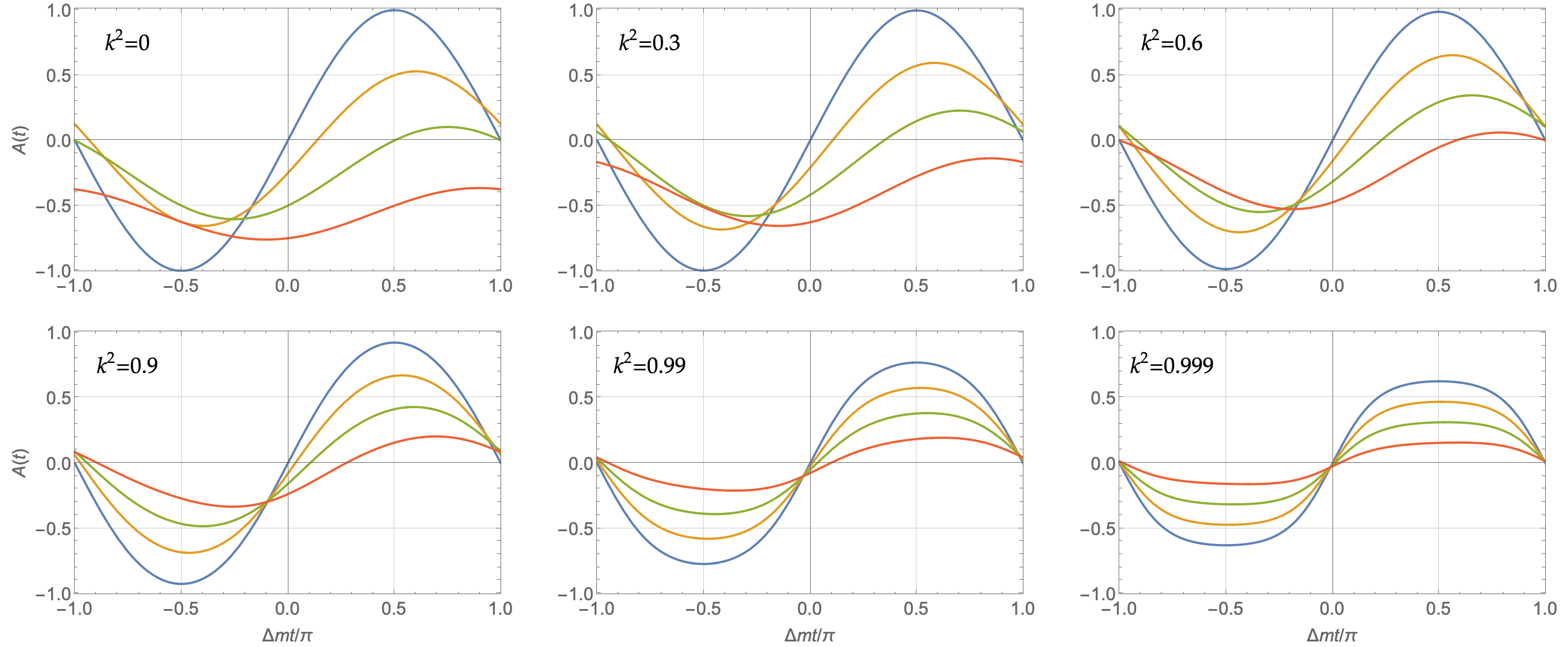
Refer to caption
Figure 8: Graphs of A​(Δ​m​t)𝐮Δ𝑚𝑡A(\Delta m\,t) for 2​AL​AH/(AL2+AH2)=12subscript𝐮𝐿subscriptđŽđ»superscriptsubscript𝐮𝐿2superscriptsubscriptđŽđ»212A_{L}A_{H}/(A_{L}^{2}+A_{H}^{2})=1, λ=0𝜆0\lambda=0, η=π/2𝜂𝜋2\eta=\pi/2. The four curves in each graph are for Ο=0𝜉0\xi=0 (blue), Ο=π/6𝜉𝜋6\xi=\pi/6 (yellow), Ο=π/4𝜉𝜋4\xi=\pi/4 (green), and Ο=π/3𝜉𝜋3\xi=\pi/3 (red). The canonical QM case is k2=0superscript𝑘20k^{2}=0 and Ο=0𝜉0\xi=0, which is the blue curve in the leftmost graph in the upper row. When k2=0superscript𝑘20k^{2}=0, the graph becomes flat at A​(t)=−1𝐮𝑡1A(t)=-1 in the limit Ο=π/2𝜉𝜋2\xi=\pi/2.

Fit to Belle Data

Let us now use actual Belle data to constrain the deformation parameters k𝑘k and ÎŸđœ‰\xi. We use the data from [35]. We first consider the k=0𝑘0k=0 case and look at how the fit of Eq. (227) to the Belle data constrains the parameter ÎŸđœ‰\xi.

In interpreting the experimental data, one should take into account the miss-tag factors wB0subscriptđ‘€superscriptđ”0w_{B^{0}} and wBÂŻ0subscriptđ‘€superscriptÂŻđ”0w_{\overline{B}^{0}} that respectively characterizes the probability of incorrectly tagging the B0superscriptđ”0B^{0} as B0ÂŻÂŻsuperscriptđ”0\overline{B^{0}}, and vice versa. The probability amplitudes are modified to

|⟹f|B0​(t)⟩|2superscriptinner-product𝑓superscriptđ”0𝑡2\displaystyle\big{|}\langle f|B^{0}(t)\rangle\big{|}^{2} →→\displaystyle\rightarrow (1−wB0)​|⟹f|B0​(t)⟩|2+wBÂŻ0​|⟹f|BÂŻ0​(t)⟩|2,1subscriptđ‘€superscriptđ”0superscriptinner-product𝑓superscriptđ”0𝑡2subscriptđ‘€superscriptÂŻđ”0superscriptinner-product𝑓superscriptÂŻđ”0𝑡2\displaystyle(1-w_{B^{0}})\big{|}\langle f|B^{0}(t)\rangle\big{|}^{2}+w_{\overline{B}^{0}}\big{|}\langle f|\overline{B}^{0}(t)\rangle\big{|}^{2}\;, (232)
|⟹f|B0¯​(t)⟩|2superscriptinner-product𝑓¯superscriptđ”0𝑡2\displaystyle\big{|}\langle f|\overline{B^{0}}(t)\rangle\big{|}^{2} →→\displaystyle\rightarrow (1−wBÂŻ0)​|⟹f|B0¯​(t)⟩|2+wB0​|⟹f|B0​(t)⟩|2,1subscriptđ‘€superscriptÂŻđ”0superscriptinner-product𝑓¯superscriptđ”0𝑡2subscriptđ‘€superscriptđ”0superscriptinner-product𝑓superscriptđ”0𝑡2\displaystyle(1-w_{\overline{B}^{0}})\big{|}\langle f|\overline{B^{0}}(t)\rangle|^{2}+w_{B^{0}}|\langle f|B^{0}(t)\rangle\big{|}^{2}\;, (233)

and A​(t)𝐮𝑡A(t) to

A​(t)𝐮𝑡\displaystyle A(t) →→\displaystyle\to [(1−wBÂŻ0)​|⟹f|B0¯​(t)⟩|2+wB0​|⟹f|B0​(t)⟩|2]−[(1−wB0)​|⟹f|B0​(t)⟩|2+wBÂŻ0​|⟹f|BÂŻ0​(t)⟩|2][(1−wBÂŻ0)​|⟹f|B0¯​(t)⟩|2+wB0​|⟹f|B0​(t)⟩|2]+[(1−wB0)​|⟹f|B0​(t)⟩|2+wBÂŻ0​|⟹f|BÂŻ0​(t)⟩|2]delimited-[]1subscriptđ‘€superscriptÂŻđ”0superscriptinner-product𝑓¯superscriptđ”0𝑡2subscriptđ‘€superscriptđ”0superscriptinner-product𝑓superscriptđ”0𝑡2delimited-[]1subscriptđ‘€superscriptđ”0superscriptinner-product𝑓superscriptđ”0𝑡2subscriptđ‘€superscriptÂŻđ”0superscriptinner-product𝑓superscriptÂŻđ”0𝑡2delimited-[]1subscriptđ‘€superscriptÂŻđ”0superscriptinner-product𝑓¯superscriptđ”0𝑡2subscriptđ‘€superscriptđ”0superscriptinner-product𝑓superscriptđ”0𝑡2delimited-[]1subscriptđ‘€superscriptđ”0superscriptinner-product𝑓superscriptđ”0𝑡2subscriptđ‘€superscriptÂŻđ”0superscriptinner-product𝑓superscriptÂŻđ”0𝑡2\displaystyle\dfrac{\Big{[}(1-w_{\overline{B}^{0}})\big{|}\langle f|\overline{B^{0}}(t)\rangle|^{2}+w_{B^{0}}|\langle f|B^{0}(t)\rangle\big{|}^{2}\Big{]}-\Big{[}(1-w_{B^{0}})\big{|}\langle f|B^{0}(t)\rangle\big{|}^{2}+w_{\overline{B}^{0}}\big{|}\langle f|\overline{B}^{0}(t)\rangle\big{|}^{2}\Big{]}}{\Big{[}(1-w_{\overline{B}^{0}})\big{|}\langle f|\overline{B^{0}}(t)\rangle|^{2}+w_{B^{0}}|\langle f|B^{0}(t)\rangle\big{|}^{2}\Big{]}+\Big{[}(1-w_{B^{0}})\big{|}\langle f|B^{0}(t)\rangle\big{|}^{2}+w_{\overline{B}^{0}}\big{|}\langle f|\overline{B}^{0}(t)\rangle\big{|}^{2}\Big{]}} (235)
=Δ​w+D​A​(t),absentÎ”đ‘€đ·đŽđ‘Ą\displaystyle=\;\Delta w+DA(t)\;,\vphantom{\bigg{|}}

where D=1−2​⟹wâŸ©đ·12delimited-âŸšâŸ©đ‘€D=1-2\langle w\rangle is the dilution factor, ⟹w⟩=(wB0+wB0ÂŻ)/2delimited-âŸšâŸ©đ‘€subscriptđ‘€superscriptđ”0subscriptđ‘€ÂŻsuperscriptđ”02\langle w\rangle=(w_{B^{0}}+w_{\overline{B^{0}}})/2 the average miss-tag probability, and Δ​w=wB0−wBÂŻ0Î”đ‘€subscriptđ‘€superscriptđ”0subscriptđ‘€superscriptÂŻđ”0\Delta w=w_{B^{0}}-w_{\overline{B}^{0}}.

The dilution factor Dđ·D simply suppresses the overall amplitude 2​AL​AH/(AL2+AH2)2subscript𝐮𝐿subscriptđŽđ»superscriptsubscript𝐮𝐿2superscriptsubscriptđŽđ»22A_{L}A_{H}/(A_{L}^{2}+A_{H}^{2}) of A​(t)𝐮𝑡A(t). Since 2​AL​AH/(AL2+AH2)2subscript𝐮𝐿subscriptđŽđ»superscriptsubscript𝐮𝐿2superscriptsubscriptđŽđ»22A_{L}A_{H}/(A_{L}^{2}+A_{H}^{2}) is already restricted to have magnitude smaller than one, the presence of Dđ·D does not add any new constraints. The difference in miss-tag probabilities, Δ​wÎ”đ‘€\Delta w, leads to an offset of A​(t)𝐮𝑡A(t) in the vertical direction. This is known to be negligibly small for analyses involving a low number of events, and indeed we find that its preferred value when included in our fits is approximately zero. Therefore, we set Δ​w=0Î”đ‘€0\Delta w=0 in the following.

Firstly, we fit Eq. (227) to the Belle data allowing 2​AL​AH/(AL2+AH2)2subscript𝐮𝐿subscriptđŽđ»superscriptsubscript𝐮𝐿2superscriptsubscriptđŽđ»22A_{L}A_{H}/(A_{L}^{2}+A_{H}^{2}), (η−λ)𝜂𝜆(\eta-\lambda), and ÎŸđœ‰\xi to float. The mass difference Δ​mΔ𝑚\Delta m is set to the current world average, Eq. (189), from the Review of Particle Properties [42]. The minimum of the χ2superscript𝜒2\chi^{2} is found to be 15.0615.0615.06 for 24−324324-3 degrees of freedom at

2​AL​AHAL2+AH2=±0.4006,η−λπ={+0.5496−0.4504,Ο= 0,formulae-sequence2subscript𝐮𝐿subscriptđŽđ»superscriptsubscript𝐮𝐿2superscriptsubscriptđŽđ»2plus-or-minus0.4006formulae-sequence𝜂𝜆𝜋cases0.5496otherwise0.4504otherwise𝜉 0\dfrac{2A_{L}A_{H}}{A_{L}^{2}+A_{H}^{2}}\;=\;\pm 0.4006\;,\qquad\dfrac{\eta-\lambda}{\pi}\;=\;\begin{cases}+0.5496\\ -0.4504\end{cases},\qquad\xi\;=\;0\;, (236)

that is, canonical QM is preferred over a non-zero ÎŸđœ‰\xi. The best-fit curve is shown against the data of [35] in FIG. 10 as the canonical QM fit. The likelihood function for ÎŸđœ‰\xi is shown in FIG. 9. It has the characteristic feature that it suddenly drops to zero around Ο/π∌0.2similar-to𝜉𝜋0.2\xi/\pi\sim 0.2. This drop is caused by the amplitude |2​AL​AH/(AL2+AH2)|≀12subscript𝐮𝐿subscriptđŽđ»superscriptsubscript𝐮𝐿2superscriptsubscriptđŽđ»21|2A_{L}A_{H}/(A_{L}^{2}+A_{H}^{2})|\leq 1 being unable to compensate for the flattening of the oscillation curve as ÎŸđœ‰\xi is increased beyond this point. This is similar to the atmospheric neutrino analysis in which sin2⁥2​Ξ≀1superscript22𝜃1\sin^{2}2\theta\leq 1 was unable to compensate for an increase in ÎŸđœ‰\xi, and the resulting suppression of cΟ2superscriptsubscript𝑐𝜉2c_{\xi}^{2}. From this likelihood curve, we find the upper bounds on ÎŸđœ‰\xi to be

Οπ< 0.098​(1​σ, 68%),0.168​(2​σ, 95%),0.192​(3​σ, 99.7%).𝜉𝜋0.0981𝜎percent680.1682𝜎percent950.1923𝜎percent99.7\dfrac{\xi}{\pi}\;<\;0.098\;\;(1\sigma,\;68\%),\qquad 0.168\;\;(2\sigma,\;95\%),\qquad 0.192\;\;(3\sigma,\;99.7\%)\;. (237)

Note that these are weaker than the atmospheric neutrino bounds given in Eq. (125).
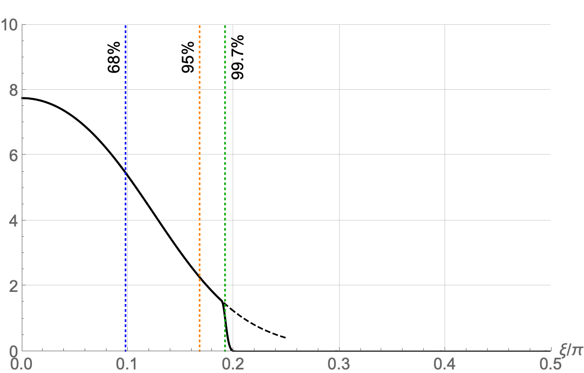
Refer to caption
Figure 9: The likelihood function for ÎŸđœ‰\xi for the k=0𝑘0k=0 case. The vertical axis is in units so that the area underneath the curve is one. The sudden drop at Ο/π∌0.2similar-to𝜉𝜋0.2\xi/\pi\sim 0.2 is due to the amplitude |2​AL​AH/(AL2+AH2)|≀12subscript𝐮𝐿subscriptđŽđ»superscriptsubscript𝐮𝐿2superscriptsubscriptđŽđ»21|2A_{L}A_{H}/(A_{L}^{2}+A_{H}^{2})|\leq 1 being unable to compensate for the flattening of the oscillation curve as ÎŸđœ‰\xi is increased, cf. FIG. 8. The dashed line indicates how the likelihood function would have looked without the amplitude constraint. The vertical dotted lines indicate the locations of the 1​σ1𝜎1\sigma (68%), 2​σ2𝜎2\sigma (95%), and 3​σ3𝜎3\sigma (99.7%) bounds.
Refer to caption
Figure 10: Time-dependent CP asymmetry data from Belle [35] fitted with Nambu QM (black solid) and canonical QM (red dashed). For the Nambu QM curve, k2=0.957superscript𝑘20.957k^{2}=0.957 and Ο=0𝜉0\xi=0. The value of the χ2superscript𝜒2\chi^{2} per degree of freedom at the best fit point is 14.32/(24−5)=0.7514.322450.7514.32/(24-5)=0.75 for Nambu QM, and 15.06/(24−2)=0.6815.062420.6815.06/(24-2)=0.68 for canonical QM.
Refer to caption
Refer to caption
Figure 11: k2superscript𝑘2k^{2}-ÎŸđœ‰\xi contour plot showing the 1​σ1𝜎1\sigma(68%), 2​σ2𝜎2\sigma(95%) and 3​σ3𝜎3\sigma(99.7%) likelihood contours for the Belle fit. The red dot denotes the point which minimizes the χ2superscript𝜒2\chi^{2}. The right figure is a blowup of the region 0.99<k2<10.99superscript𝑘210.99<k^{2}<1.

Next, we fit Eq. (226) to the Belle data to constrain both ÎŸđœ‰\xi and k𝑘k. The fit parameters are 2​AL​AH/(AL2+AH2)2subscript𝐮𝐿subscriptđŽđ»superscriptsubscript𝐮𝐿2superscriptsubscriptđŽđ»22A_{L}A_{H}/(A_{L}^{2}+A_{H}^{2}), Î»đœ†\lambda, Î·đœ‚\eta, k2superscript𝑘2k^{2}, and ÎŸđœ‰\xi. The mass difference Δ​mΔ𝑚\Delta m is set to Eq. (189). The minimum of the χ2superscript𝜒2\chi^{2} is found to be 14.3214.3214.32 for 24−5=192451924-5=19 degrees of freedom when

2​AL​AHAL2+AH2=±0.4403,Θ1​(λ,η)π={+0.5469−0.4531,k2= 0.957,Ο= 0.formulae-sequence2subscript𝐮𝐿subscriptđŽđ»superscriptsubscript𝐮𝐿2superscriptsubscriptđŽđ»2plus-or-minus0.4403formulae-sequencesubscriptΘ1𝜆𝜂𝜋cases0.5469otherwise0.4531otherwiseformulae-sequencesuperscript𝑘20.957𝜉 0\dfrac{2A_{L}A_{H}}{A_{L}^{2}+A_{H}^{2}}\;=\;\pm 0.4403\;,\qquad\dfrac{\Theta_{1}(\lambda,\eta)}{\pi}\;=\;\begin{cases}+0.5469\\ -0.4531\end{cases},\qquad k^{2}\;=\;0.957\;,\qquad\xi\;=\;0\;. (238)

Θ2​(λ,η)subscriptΘ2𝜆𝜂\Theta_{2}(\lambda,\eta) is unconstrained due to the best fit value of ÎŸđœ‰\xi being zero, leading to degeneracies on the (λ,η)𝜆𝜂(\lambda,\eta) plane. The best fit curve is shown in FIG. 10 against the data and the canonical QM best fit. The likelihood contours on the k2superscript𝑘2k^{2}-ÎŸđœ‰\xi plane are shown in FIG. 11. Note that the best fit point is at Ο=0𝜉0\xi=0 and k2=0.957superscript𝑘20.957k^{2}=0.957, exceptionally close to the maximum allowed value of k2superscript𝑘2k^{2}. This is due to the fact that the data prefers an oscillation which slightly deviates from the sinusoidal, as can be seen in FIG. 10, while Jacobi’s elliptical functions show such deviations in a noticeable way only as k2superscript𝑘2k^{2} approaches 1. This leads to k2superscript𝑘2k^{2} being only very weakly constrained. The 3​σ3𝜎3\sigma contour on FIG. 11 traces a precipice in the likelihood function along which it plummets to zero, just as in the k=0𝑘0k=0 case, cf. FIG. 9. This is again due to the constraint |2​AL​AH/(AL2+AH2)|≀12subscript𝐮𝐿subscriptđŽđ»superscriptsubscript𝐮𝐿2superscriptsubscriptđŽđ»21|2A_{L}A_{H}/(A_{L}^{2}+A_{H}^{2})|\leq 1.

VI Summary and Discussion

In this paper, we have reviewed how Nambu QM [2] extends canonical QM via its geometrical formulation [29, 30, 32, 31, 33, 34]. All states are expressed as superpositions of energy eigenstates with coefficients that have magnitudes and “phases.” The extension involves generalizing the concept of the “phase” to a map from S1superscript𝑆1S^{1} (a circle) to S2superscript𝑆2S^{2} (a sphere). The 2​N2𝑁2N dimensional KĂ€hler manifold of geometric QM for N𝑁N energy eigenstates is generalized to a 3​N3𝑁3N dimensional manifold. Canonical QM corresponds to the “phase” being a map from S1superscript𝑆1S^{1} to the equator of S2superscript𝑆2S^{2}.

Deviations of the map from the equator is described by two deformation parameters ÎŸđœ‰\xi and k𝑘k. The trajectory of the map is assumed to follow the path of the angular momentum of an asymmetric top, the motion of which can be described by the triple Nambu bracket [3] with two conserved quantities, one of which maintains the “phase” vector on the surface of S2superscript𝑆2S^{2}. The dependence of the 3D “phase” vector on the phase parameter is described by Jacobi’s elliptical functions cn​(u,k)cn𝑱𝑘\mathrm{cn}(u,k), sn​(u,k)sn𝑱𝑘\mathrm{sn}(u,k), and dn​(u,k)dn𝑱𝑘\mathrm{dn}(u,k), where k𝑘k is the eccentricity of the ellipse from which these function are defined.

Under this deformation, the coefficients of the energy eigenstates are no longer elements of a field or division algebra since the addition of coefficients is ill defined. The inner product defined for the extension is also not invariant under generic phase shifts of the coefficients. Therefore, the projective vector space structure of the state space of canonical QM is lost. Since the coefficients do not add, there is no path-integral formulation of the Nambu extension in which such a coefficient is associated with each path, and the paths interfere with each other via superposition. Nevertheless, the energy eigenstates with those coefficients do interfere allowing for oscillation phenomena, which deform those of canonical QM.

We have used atmospheric neutrino [38] and Belle [35] data to constrain the deformation parameters ÎŸđœ‰\xi and k𝑘k, as shown in FIGS. 5 and 11. Of the two deformation parameters ÎŸđœ‰\xi is the better constrained, the 3​σ3𝜎3\sigma upper bounds for the k=0𝑘0k=0 case being ∌0.07​πsimilar-toabsent0.07𝜋\sim 0.07\pi and ∌0.2​πsimilar-toabsent0.2𝜋\sim 0.2\pi for atmospheric neutrinos and Belle, respectively, cf. Eq. (125) and (237). This is due to the parameter ÎŸđœ‰\xi suppressing oscillations as it is increased from 0 to π/2𝜋2\pi/2, while the overall amplitude (sin2⁥2​ξsuperscript22𝜃\sin^{2}2\theta in the case of atmospheric neutrinos and 2​AL​AH/(AL2+AH2)2subscript𝐮𝐿subscriptđŽđ»superscriptsubscript𝐮𝐿2superscriptsubscriptđŽđ»22A_{L}A_{H}/(A_{L}^{2}+A_{H}^{2}) in the case of B0superscriptđ”0B^{0}-B0ÂŻÂŻsuperscriptđ”0\overline{B^{0}} oscillations, which are both bounded by 1) is unable to compensate for it. The somewhat surprising result is that the bound from atmospheric neutrinos is stronger than the Belle bound.

The bound on k2superscript𝑘2k^{2} in contrast is very weak. This is due to k2superscript𝑘2k^{2} causing significant deviations of the oscillation functions from the sinusoidal only when k2superscript𝑘2k^{2} is very close to one. Indeed, the best fit value to the Belle data was k2=0.957superscript𝑘20.957k^{2}=0.957, Eq. (238), due to the data preferring a slight deviation of the oscillation curve from the sinusoidal. See FIG. 10. However, this was based on a simplified oscillation formula which resulted due to the sum of the eigenfrequencies of the interfering energy eigenstates being much larger that the difference, allowing us to average out the fast oscillations. For situations in which the sum and difference of the frequencies are much closer to each other, there will be significant deviations from sinusoidal oscillations at the frequency difference, and we expect the bound on k2superscript𝑘2k^{2} to be much stronger. Furthermore, the k=0𝑘0k=0 case is preferred theoretically, since it will allow for phase changes of the energy eigenstates without affecting physical probabilities, justifying the somewhat arbitrary phase choices in Eqs. (68) and (168).

In addition to the loss of the projective vector space structure of the state space, Nambu QM has other shortcomings as well. First, unstable states cannot be made to decay by giving them complex energy eigenvalues. This is due to the doubly periodic nature of the Jacobi elliptic functions which are periodic in the imaginary direction as well as the real. Thus, we must let the amplitudes of the coefficients decay exponentially by hand. Second, since the Nambu extension relies on a fixed energy-eigenstate basis, it is not clear how it should be applied to situations in which the energy eigenstates and their respective eigenvalues are themselves time-dependent. For instance, when considering matter effects on neutrino oscillations, the eigenstates of the neutrino Hamiltonian change depending on the background electron density. This is the reason why we did not analyze neutrino oscillations directly in this paper.

Despite these drawbacks, Nambu QM has many interesting features beyond the deformation of oscillations that can be constrained by experiment. First, when k=0𝑘0k=0 but Ο≠0𝜉0\xi\neq 0, the inner product becomes invariant under a global phase shift of all states by a common phase. Thus, if we gauge the theory it will become a U​(1)𝑈1U(1) gauge theory in which all states carry a common U​(1)𝑈1U(1) charge. This may provide a new way to quantize U​(1)𝑈1U(1) charges without the need to embed the theory into a non-Abelian gauge theory.

Second, the parameter choice Ο=π/2𝜉𝜋2\xi=\pi/2, k=0𝑘0k=0 leads to a model which is pseudo-classical, i.e. all oscillations vanish in this limit (though interferences do not). Thus Nambu QM provides a framework in which one can interpolate between quantum and classical-like behavior continuously by tuning the deformation parameter ÎŸđœ‰\xi. This property may allow us to study how the Leggett-Garg inequalities [44, 45, 46, 47, 48] set in as pseudo-classicality is approached.

We note that the loss of addition of the “numbers” that constitute the state coefficients may be what is necessary to render a quantum-like theory classical (or pseudo-classical). Indeed, in [15] it has been shown that in the q→1→𝑞1q\to 1 limit of đ”œqsubscriptđ”œđ‘ž\mathbb{F}_{q}QM [12, 13, 14, 16], which is a quantum mechanical model constructed over the finite Galois field đ”œqsubscriptđ”œđ‘ž\mathbb{F}_{q}, the theory behaves “classically,” while đ”œqsubscriptđ”œđ‘ž\mathbb{F}_{q} becomes the so-called “field with one element” đ”œ1subscriptđ”œ1\mathbb{F}_{1}, or đ”œunsubscriptđ”œun\mathbb{F}_{\text{un}} [49], for which the elements multiply but do not add.

Third, it may be possible to construct a model with Sorkin’s triple-path interference [27, 50, 51] using the Nambu approach. In both canonical and Nambu QM, interference between different energy eigenstates is pairwise due to the Born Rule. They result from the cross terms that appear in the squares of the symmetric and anti-symmetric parts of the inner product, namely:

(Ω→n⋅ι→n)​(Ω→m⋅ι→m),and(Ω→n×ι→n)⋅(Ω→m×ι→m),n≠m.⋅subscript→Ω𝑛subscript→ι𝑛⋅subscript→Ω𝑚subscript→ι𝑚and⋅subscript→Ω𝑛subscript→ι𝑛subscript→Ω𝑚subscript→ι𝑚𝑛𝑚(\vec{\Phi}_{n}\cdot\vec{\Psi}_{n})(\vec{\Phi}_{m}\cdot\vec{\Psi}_{m})\;,\quad\mbox{and}\quad(\vec{\Phi}_{n}\times\vec{\Psi}_{n})\cdot(\vec{\Phi}_{m}\times\vec{\Psi}_{m})\;,\qquad n\neq m\;. (239)

However, in the Nambu extension (Ω→n×ι→n)subscript→Ω𝑛subscript→ι𝑛(\vec{\Phi}_{n}\times\vec{\Psi}_{n}) is a 3D vector, allowing us to construct the 3D volume

(Ω→n×ι→n)⋅[(Ω→m×ι→m)×(Ω→k×ι→k)],n≠m≠k≠n,⋅subscript→Ω𝑛subscript→ι𝑛delimited-[]subscript→Ω𝑚subscript→ι𝑚subscript→Ω𝑘subscript→ι𝑘𝑛𝑚𝑘𝑛\big{(}\vec{\Phi}_{n}\times\vec{\Psi}_{n}\big{)}\cdot\Big{[}\big{(}\vec{\Phi}_{m}\times\vec{\Psi}_{m}\big{)}\times\big{(}\vec{\Phi}_{k}\times\vec{\Psi}_{k}\big{)}\Big{]}\;,\qquad n\neq m\neq k\neq n\;, (240)

which could be interpreted as the interference of the n𝑛nth, m𝑚mth, and k𝑘kth energy eigenstates. If such a term can be incorporated into a unitary model, we would have an extension of canonical QM with triple-path interference. Note that the existence of such a model is crucial in experimentally probing the validity of the Born rule [52, 50] as an alternative theory against which to compare canonical QM.

Furthermore, though we only consider an extension of the “phase” to a map from S1superscript𝑆1S^{1} to S2superscript𝑆2S^{2}, the Nambu bracket [3] exists for any number of dimensions and it can be used to extend the “phase” to a map from S1superscript𝑆1S^{1} to Sn−1superscript𝑆𝑛1S^{n-1}, n=4,5,⋯𝑛45⋯n=4,5,\cdots. In those higher dimensional extensions, the phase vector will be n𝑛n-dimensional, and n𝑛n-dimensional hypervolumes can be constructed, which could correspond to n𝑛n-path interferences. Therefore, the possibility exists for a ladder of models, the n𝑛n-dimensional case possessing Sorkin’s multi-path interference up to the n𝑛nth order. However, if one insists on the top-like behavior of the phase vector, then one may need to jump to 7D [53, 54, 55, 56] in which the model will have connections to octonions [57].

If we do not restrict our attention to models in which the phase vector is top-like, then even in the 3D case we can use “phase” maps from S1superscript𝑆1S^{1} to S2superscript𝑆2S^{2} that are different from what was used in this paper. For instance, we could let the phase vector of each energy eigenstate follow different great circles on S2superscript𝑆2S^{2}. Each choice of “phase” map will lead to a different phenomenology from what was discussed.

The possibility of multi-path interferences also suggests the relevance of Nambu QM to the quantization of gravity. Indeed, in the new approach to quantum gravity dubbed “gravitization of quantum theory” [58, 59], the phenomena of triple and higher order interference are naturally expected to occur [51]. The reason for this stems from the fact that “gravitization of quantum theory” by definition implies a dynamical geometry of quantum theory, and thus the generalization of the Born rule, which is tied to the canonical geometry of complex projective spaces. This canonical geometry is maximally symmetric and via the Born rule it precludes any intrinsic triple and higher order interference. However, given the non-linear and non-polynomial nature of gravitational interaction, it is expected that “gravitization of quantum theory” will lead to triple and higher interference of arbitrary order.

Other avenues worth exploring include the quantum brachistochrone problem, which is usually stated as follows: Find the Hamiltonian that takes one from a given initial state to a given final state in the least amount of time, under the constraint that the difference between the largest and the smallest eigenvalues of the Hamiltonian is fixed [60, 61, 62, 63]. Since we have not introduced a Hamiltonian operator in Nambu QM, and also since we can expect transition speeds to depend on the sums of energy eigenvalues as well as the differences when k≠0𝑘0k\neq 0, the problem must be restated somewhat to: Find the energy spectrum that takes one from a given initial state to a given final state in the least amount of time, under the constraint that the largest and the smallest energy eigenvalues are fixed. In particular, how does the answer depend on k𝑘k and ÎŸđœ‰\xi and what happens in the pseudo-classical limit k=0𝑘0k=0, Ο→π/2→𝜉𝜋2\xi\to\pi/2? Answering this will provide us with a deeper understanding of the dynamics of Nambu QM, and perhaps illuminate what happens in the classical limit of a quantum theory.

Classical Nambu theory fits into the general Hamiltonian framework of the principle of least action ή​S=0𝛿𝑆0\delta S=0, where the action of classical Nambu dynamics is the integral of a 2-form involving 2 Hamiltonians [4] (as opposed to the integral of a 1-form involving one Hamiltonian, valid in canonical classical theory). In general, one has integrals over n𝑛n-forms, with n𝑛n-Hamiltonians. The corresponding quantum theory can be formulated as an ℏPlanck-constant-over-2-pi\hbar deformation of the classical action principle, by invoking the Schwinger variational principle ÎŽS⋅=iℏή⋅\delta S\cdot=i\hbar\delta\cdot, where in the usual case one acts (ή𝛿\delta) on a complex wavefunction, or alternatively the real and imaginary parts of the wave function, respectively. The real and imaginary parts of the wavefunctions are dual to each other in this formulation that gives the canonical Schrödinger evolution. In quantum Nambu theory, the action ή𝛿\delta is on one of the components of a three-component (vector-like) wavefunction, where the dual to each component is given by the cyclic product of the other two components. Obviously this can be generalized to n𝑛n-components. In this case the variation of the action ή​S𝛿𝑆\delta S, in general, involves n𝑛n Hamiltonians of the Nambu dynamics. This general formulation leads in principle to a new view of how probabilities are calculated in Nambu quantum theory. From this point of view, Nambu quantum theory fits into a more general understanding of quantum mechanics as quantum measure theory [27], with general probabilities related to triple [50] and higher order interference phenomena [51].

In this context another curious question is what happens when we discretize the “phase” space variables of Nambu QM. This question is worth exploring especially in connection to Spekkens’ toy model [64] and its generalization, dubbed Quasi-quantization [65], in which one considers classical physical systems and imposes a limitation on the amount of knowledge that can be possessed by an observer about those systems. The theory derived from those assumptions is able to qualitatively reproduce various phenomena that are ordinarily considered characteristic of quantum theory. For instance, the version of such theory in which the phase space variables p𝑝p and q𝑞q are restricted to take on values in đ”œ2subscriptđ”œ2\mathbb{F}_{2} can reproduce a large subset of phenomena associated with quantum spins. Among the phenomena reproduced therein, the ones that are of most interest to us are coherent superposition and interference, owing to our goal of modeling triple-path interference. As such, our future work will explore Quasi-quantization of theories with three “phase” space variables in general and their discrete version in particular. However, we need to have a better understanding of the third “phase” space variable before attempting this study. This is because the analog of epistemic restriction in quantum theory is Heisenberg’s uncertainty principle and trying to define its three-variable version deserves careful consideration.

There remain numerous avenues to be pursued in further development and understanding of Nambu QM. We intend to address these possibilities in our forthcoming publications.

VII Acknowledgements

The authors would like to thank L. Piilonen for helpful communications pertaining to the B0superscriptđ”0B^{0}-B0ÂŻÂŻsuperscriptđ”0\overline{B^{0}} oscillation measurements at Belle. Discussions with C. H. Tze are also gratefully acknowledged. D. Minic and T. Takeuchi thank the Julian Schwinger Foundation and the U.S. Department of Energy (DE-SC0020262) for support.

Appendix A Classical Nambu Dynamics

Here we review some properties of the Poisson and Nambu brackets.

A.1 Poisson Bracket

If we denote

q1=q,q2=p,formulae-sequencesubscript𝑞1𝑞subscript𝑞2𝑝q_{1}\;=\;q\;,\qquad q_{2}\;=\;p\;, (241)

then the Poisson bracket can be written as

{A,B}=∂A∂q​∂B∂p−∂A∂p​∂B∂q=Δi​j​∂A∂qi​∂B∂qj,đŽđ”đŽđ‘žđ”đ‘đŽđ‘đ”đ‘žsubscript𝜀𝑖𝑗𝐮subscriptđ‘žđ‘–đ”subscript𝑞𝑗\{A,B\}\;=\;\dfrac{\partial A}{\partial q}\,\dfrac{\partial B}{\partial p}-\dfrac{\partial A}{\partial p}\,\dfrac{\partial B}{\partial q}\;=\;\varepsilon_{ij}\,\dfrac{\partial A}{\partial q_{i}}\,\dfrac{\partial B}{\partial q_{j}}\;, (242)

where Δi​jsubscript𝜀𝑖𝑗\varepsilon_{ij} is the totally antisymmetric tensor with Δ12=1subscript𝜀121\varepsilon_{12}=1 . The Poisson bracket has the following properties:

  1. 1.

    Anti-symmetry:

    {A1,A2}=−{A2,A1}.subscript𝐮1subscript𝐮2subscript𝐮2subscript𝐮1\{A_{1},A_{2}\}\;=\;-\{A_{2},A_{1}\}\;. (243)
  2. 2.

    Leibniz Rule (the operator {A1,∗}subscript𝐮1\{A_{1},*\} is a derivative acting on ∗*) :

    {A1,A2​A3}={A1,A2}​A3+A2​{A1,A3}.subscript𝐮1subscript𝐮2subscript𝐮3subscript𝐮1subscript𝐮2subscript𝐮3subscript𝐮2subscript𝐮1subscript𝐮3\{A_{1},A_{2}A_{3}\}\;=\;\{A_{1},A_{2}\}A_{3}+A_{2}\{A_{1},A_{3}\}\;. (244)
  3. 3.

    Fundamental Identity:

    {A1,{A2,A3}}+{A2,{A3,A1}}+{A3,{A1,A2}}= 0,subscript𝐮1subscript𝐮2subscript𝐮3subscript𝐮2subscript𝐮3subscript𝐮1subscript𝐮3subscript𝐮1subscript𝐮2 0\{A_{1},\{A_{2},A_{3}\}\}+\{A_{2},\{A_{3},A_{1}\}\}+\{A_{3},\{A_{1},A_{2}\}\}\;=\;0\;, (245)

    which can also be written as

    {A1,{A2,A3}}={{A1,A2},A3}+{A2,{A1,A3}},subscript𝐮1subscript𝐮2subscript𝐮3subscript𝐮1subscript𝐮2subscript𝐮3subscript𝐮2subscript𝐮1subscript𝐮3\{A_{1},\{A_{2},A_{3}\}\}\;=\;\{\{A_{1},A_{2}\},A_{3}\}+\{A_{2},\{A_{1},A_{3}\}\}\;, (246)

    which is the Leibniz rule of the derivative {A1,∗}subscript𝐮1\{A_{1},*\} acting on {A2,A3}subscript𝐮2subscript𝐮3\{A_{2},A_{3}\}.

The equation of motion of observable FđčF is

d​Fd​t=−{H,F}={F,H},𝑑đčđ‘‘đ‘Ąđ»đčđčđ»\dfrac{dF}{dt}\;=\;-\{H,F\}\;=\;\{F,H\}\;, (247)

where Hđ»H is the Hamiltonian. The operator −{H,∗}={∗,H}đ»đ»-\{H,*\}=\{*,H\} is a derivative operator acting on ∗*. For example, if

H=ω2​(q12+q22),đ»đœ”2superscriptsubscript𝑞12superscriptsubscript𝑞22H\;=\;\dfrac{\omega}{2}\left(q_{1}^{2}+q_{2}^{2}\right)\;, (248)

then

q˙1subscript˙𝑞1\displaystyle\dot{q}_{1} =\displaystyle= {q1,H}=ω​q2,subscript𝑞1đ»đœ”subscript𝑞2\displaystyle\{q_{1},H\}\;=\;\omega q_{2}\;, (249)
q˙2subscript˙𝑞2\displaystyle\dot{q}_{2} =\displaystyle= {q2,H}=−ω​q1,subscript𝑞2đ»đœ”subscript𝑞1\displaystyle\{q_{2},H\}\;=\;-\omega q_{1}\;, (250)

which are the usual equations of motion of the harmonic oscillator.

A.2 Nambu Bracket

Consider three classical variables which we write q1subscript𝑞1q_{1}, q2subscript𝑞2q_{2}, and q3subscript𝑞3q_{3}. Define the order 3 Nambu bracket as

{A,B,C}=Δi​j​k​∂A∂qi​∂B∂qj​∂C∂qk,đŽđ”đ¶subscript𝜀𝑖𝑗𝑘𝐮subscriptđ‘žđ‘–đ”subscriptđ‘žđ‘—đ¶subscript𝑞𝑘\{A,B,C\}\;=\;\varepsilon_{ijk}\,\dfrac{\partial A}{\partial q_{i}}\,\dfrac{\partial B}{\partial q_{j}}\,\dfrac{\partial C}{\partial q_{k}}\;, (251)

where Δi​j​ksubscript𝜀𝑖𝑗𝑘\varepsilon_{ijk} is the totally antisymmetric tensor with Δ123=1subscript𝜀1231\varepsilon_{123}=1. This object has the following properties:

  1. 1.

    Skew-symmetry:

    {A1,A2,A3}=(−1)ϔ​(p)​{Ap​(1),Ap​(2),Ap​(3)},subscript𝐮1subscript𝐮2subscript𝐮3superscript1italic-Ï”đ‘subscript𝐮𝑝1subscript𝐮𝑝2subscript𝐮𝑝3\{A_{1},A_{2},A_{3}\}\;=\;(-1)^{\epsilon(p)}\{A_{p(1)},A_{p(2)},A_{p(3)}\}\;, (252)

    where ϔ​(p)italic-Ï”đ‘\epsilon(p) is the signature of the permutation p𝑝p.

  2. 2.

    Leibniz Rule (the operator {A1,A2,∗}subscript𝐮1subscript𝐮2\{A_{1},A_{2},*\} is a derivative acting on ∗*) :

    {A1,A2,A3​A4}={A1,A2,A3}​A4+A3​{A1,A2,A4}.subscript𝐮1subscript𝐮2subscript𝐮3subscript𝐮4subscript𝐮1subscript𝐮2subscript𝐮3subscript𝐮4subscript𝐮3subscript𝐮1subscript𝐮2subscript𝐮4\{A_{1},A_{2},A_{3}A_{4}\}\;=\;\{A_{1},A_{2},A_{3}\}A_{4}+A_{3}\{A_{1},A_{2},A_{4}\}\;. (253)
  3. 3.

    Fundamental Identity:

    {A1,A2,{A3,A4,A5}}subscript𝐮1subscript𝐮2subscript𝐮3subscript𝐮4subscript𝐮5\displaystyle\{A_{1},A_{2},\{A_{3},A_{4},A_{5}\}\} (254)
    =\displaystyle= {{A1,A2,A3},A4,A5}+{A3,{A1,A2,A4},A5}+{A3,A4,{A1,A2,A5}}.subscript𝐮1subscript𝐮2subscript𝐮3subscript𝐮4subscript𝐮5subscript𝐮3subscript𝐮1subscript𝐮2subscript𝐮4subscript𝐮5subscript𝐮3subscript𝐮4subscript𝐮1subscript𝐮2subscript𝐮5\displaystyle\{\{A_{1},A_{2},A_{3}\},A_{4},A_{5}\}+\{A_{3},\{A_{1},A_{2},A_{4}\},A_{5}\}+\{A_{3},A_{4},\{A_{1},A_{2},A_{5}\}\}\;.\qquad\qquad (255)

    This is the Leibniz rule for the operator {A1,A2,∗}subscript𝐮1subscript𝐮2\{A_{1},A_{2},*\} acting on {A3,A4,A5}subscript𝐮3subscript𝐮4subscript𝐮5\{A_{3},A_{4},A_{5}\}.

These are analogues of the properties of the Poisson bracket listed above.

The equation of motion for Nambu dynamics is

d​Fd​t=−{H1,H2,F}.𝑑đč𝑑𝑡subscriptđ»1subscriptđ»2đč\dfrac{dF}{dt}\;=\;-\{H_{1},H_{2},F\}\;. (256)

with two Hamiltonians H1subscriptđ»1H_{1} and H2subscriptđ»2H_{2}. The operator {H1,H2,∗}subscriptđ»1subscriptđ»2\{H_{1},H_{2},*\} is a derivative operator acting on ∗*. Due to the skew-symmetry of the Nambu bracket, it is clear that

H˙1subscriptË™đ»1\displaystyle\dot{H}_{1} =\displaystyle= −{H1,H1,H2}= 0,subscriptđ»1subscriptđ»1subscriptđ»2 0\displaystyle-\{H_{1},H_{1},H_{2}\}\;=\;0\;, (257)
H˙2subscriptË™đ»2\displaystyle\dot{H}_{2} =\displaystyle= −{H1,H2,H2}= 0,subscriptđ»1subscriptđ»2subscriptđ»2 0\displaystyle-\{H_{1},H_{2},H_{2}\}\;=\;0\;, (258)

that is, both H1subscriptđ»1H_{1} and H2subscriptđ»2H_{2} are conserved. The flow generated by ternary Nambu brackets is volume-preserving, generalizing the area-preserving flow of Poisson brackets.

A.3 Asymmetric Top

As an example, let

H1subscriptđ»1\displaystyle H_{1} =\displaystyle= 12​[1I1​(q1)2+1I2​(q2)2+1I3​(q3)2],12delimited-[]1subscriptđŒ1superscriptsubscript𝑞121subscriptđŒ2superscriptsubscript𝑞221subscriptđŒ3superscriptsubscript𝑞32\displaystyle\dfrac{1}{2}\biggl{[}\dfrac{1}{I_{1}}(q_{1})^{2}+\dfrac{1}{I_{2}}(q_{2})^{2}+\dfrac{1}{I_{3}}(q_{3})^{2}\biggr{]}\;,\vphantom{\Bigg{|}} (259)
H2subscriptđ»2\displaystyle H_{2} =\displaystyle= 12​[(q1)2+(q2)2+(q3)2],12delimited-[]superscriptsubscript𝑞12superscriptsubscript𝑞22superscriptsubscript𝑞32\displaystyle\dfrac{1}{2}\Bigl{[}(q_{1})^{2}+(q_{2})^{2}+(q_{3})^{2}\Bigr{]}\;,\vphantom{\Bigg{|}} (260)

where qisubscript𝑞𝑖q_{i} (i=1,2,3)𝑖123(i=1,2,3) are the dynamical variables and IisubscriptđŒđ‘–I_{i} (i=1,2,3)𝑖123(i=1,2,3) are constants. Without loss of generality we can assume I1≀I2<I3subscriptđŒ1subscriptđŒ2subscriptđŒ3I_{1}\leq I_{2}<I_{3}. Then, the equations of motion are

q˙1subscript˙𝑞1\displaystyle\dot{q}_{1} =\displaystyle= −{q1,H1,H2}=(1I3−1I2)​q2​q3,subscript𝑞1subscriptđ»1subscriptđ»21subscriptđŒ31subscriptđŒ2subscript𝑞2subscript𝑞3\displaystyle-\left\{q_{1},H_{1},H_{2}\right\}\;=\;\left(\dfrac{1}{I_{3}}-\dfrac{1}{I_{2}}\right)q_{2}\,q_{3}\;,\vphantom{\Bigg{|}} (261)

and cyclic permutations. These can be identified with the equations of motion of the angular momentum L→=(q1,q2,q3)→𝐿subscript𝑞1subscript𝑞2subscript𝑞3\vec{L}=(q_{1},q_{2},q_{3}) of an asymmetric top with moments of inertia I1≀I2<I3subscriptđŒ1subscriptđŒ2subscriptđŒ3I_{1}\leq I_{2}<I_{3}, energy H1subscriptđ»1H_{1}, and total angular momentum squared 2​H22subscriptđ»22H_{2}, in the frame fixed to the top. The I1=I2subscriptđŒ1subscriptđŒ2I_{1}=I_{2} case is the symmetric top limit.

Since both H1subscriptđ»1H_{1} and H2subscriptđ»2H_{2} are conserved, the ellipsoid H1=constantsubscriptđ»1constantH_{1}=\text{constant} and the sphere H2=constantsubscriptđ»2constantH_{2}=\text{constant} must have an intersection in the 3D (q1,q2,q3)subscript𝑞1subscript𝑞2subscript𝑞3(q_{1},q_{2},q_{3}) space for a solution to exist. This requires the shortest axis of the ellipsoid to be shorter than the radius of the sphere while the longest axis of the ellipsoid is longer than the radius of the sphere. We assume

I1≀I2<H2H1<I3subscriptđŒ1subscriptđŒ2subscriptđ»2subscriptđ»1subscriptđŒ3I_{1}\leq I_{2}<\dfrac{H_{2}}{H_{1}}<I_{3} (262)

in which case the two intersections are respectively in the northern and southern hemispheres, and in the limit I1=I2→H2/H1subscriptđŒ1subscriptđŒ2→subscriptđ»2subscriptđ»1I_{1}=I_{2}\to H_{2}/H_{1} the intersections come together at the equator. When this condition is satisfied, the solution to the equation of motion is given by the Jacobi elliptic functions, namely:

q1​(t)subscript𝑞1𝑡\displaystyle q_{1}(t) =\displaystyle= N1​cn​(Ω​t,k),subscript𝑁1cnÎ©đ‘Ąđ‘˜\displaystyle\phantom{-}N_{1}\;\mathrm{cn}(\Omega t,k)\;,\vphantom{\big{|}} (263)
q2​(t)subscript𝑞2𝑡\displaystyle q_{2}(t) =\displaystyle= −N2​sn​(Ω​t,k),subscript𝑁2snÎ©đ‘Ąđ‘˜\displaystyle-N_{2}\;\mathrm{sn}(\Omega t,k)\;,\vphantom{\big{|}} (264)
q3​(t)subscript𝑞3𝑡\displaystyle q_{3}(t) =\displaystyle= −N3​dn​(Ω​t,k),subscript𝑁3dnÎ©đ‘Ąđ‘˜\displaystyle-N_{3}\;\mathrm{dn}(\Omega t,k)\;,\vphantom{\big{|}} (265)

where N1subscript𝑁1N_{1}, N2subscript𝑁2N_{2}, and N3subscript𝑁3N_{3} are all positive, and

Ω2superscriptΩ2\displaystyle\Omega^{2} =\displaystyle= 2​(I3−I2)​(H2−I1​H1)I1​I2​I32subscriptđŒ3subscriptđŒ2subscriptđ»2subscriptđŒ1subscriptđ»1subscriptđŒ1subscriptđŒ2subscriptđŒ3\displaystyle\dfrac{2(I_{3}-I_{2})(H_{2}-I_{1}H_{1})}{I_{1}I_{2}I_{3}}\vphantom{\Bigg{|}} (266)
=\displaystyle= 2​H1​(I3−I2)​[(H2/H1−I2)+(I2−I1)I1​I2​I3],2subscriptđ»1subscriptđŒ3subscriptđŒ2delimited-[]subscriptđ»2subscriptđ»1subscriptđŒ2subscriptđŒ2subscriptđŒ1subscriptđŒ1subscriptđŒ2subscriptđŒ3\displaystyle 2H_{1}(I_{3}-I_{2})\bigg{[}\dfrac{(H_{2}/H_{1}-I_{2})+(I_{2}-I_{1})}{I_{1}I_{2}I_{3}}\bigg{]}\;,\vphantom{\Bigg{|}} (267)
k2superscript𝑘2\displaystyle k^{2} =\displaystyle= (I2−I1)​(I3​H1−H2)(H2−I1​H1)​(I3−I2)subscriptđŒ2subscriptđŒ1subscriptđŒ3subscriptđ»1subscriptđ»2subscriptđ»2subscriptđŒ1subscriptđ»1subscriptđŒ3subscriptđŒ2\displaystyle\dfrac{(I_{2}-I_{1})(I_{3}H_{1}-H_{2})}{(H_{2}-I_{1}H_{1})(I_{3}-I_{2})}\vphantom{\Bigg{|}} (268)
=\displaystyle= [(I2−I1)(I2−I1)+(H2/H1−I2)]​[(I3−H2/H1)(I3−H2/H1)+(H2/H1−I2)].delimited-[]subscriptđŒ2subscriptđŒ1subscriptđŒ2subscriptđŒ1subscriptđ»2subscriptđ»1subscriptđŒ2delimited-[]subscriptđŒ3subscriptđ»2subscriptđ»1subscriptđŒ3subscriptđ»2subscriptđ»1subscriptđ»2subscriptđ»1subscriptđŒ2\displaystyle\bigg{[}\dfrac{(I_{2}-I_{1})}{(I_{2}-I_{1})+(H_{2}/H_{1}-I_{2})}\bigg{]}\bigg{[}\dfrac{(I_{3}-H_{2}/H_{1})}{(I_{3}-H_{2}/H_{1})+(H_{2}/H_{1}-I_{2})}\bigg{]}\;.\vphantom{\Bigg{|}} (269)

This solution traces the intersection of the sphere and ellipsoid in the southern hemisphere. Given Eq. (262), we note that 0≀k2<10superscript𝑘210\leq k^{2}<1 where k2=0superscript𝑘20k^{2}=0 if and only if I1=I2subscriptđŒ1subscriptđŒ2I_{1}=I_{2}, while k2→1→superscript𝑘21k^{2}\to 1 as I2→H2/H1→subscriptđŒ2subscriptđ»2subscriptđ»1I_{2}\to H_{2}/H_{1}, provided I1≠I2subscriptđŒ1subscriptđŒ2I_{1}\neq I_{2}.

Due to the non-linearity of Eq. (261), the normalization constants N1,N2,subscript𝑁1subscript𝑁2N_{1},N_{2}, and N3subscript𝑁3N_{3} are also fixed:

N1=2​I1​(I3​H1−H2)(I3−I1),N2=2​I2​(I3​H1−H2)(I3−I2),N3=2​I3​(H2−I1​H1)(I3−I1).formulae-sequencesubscript𝑁12subscriptđŒ1subscriptđŒ3subscriptđ»1subscriptđ»2subscriptđŒ3subscriptđŒ1formulae-sequencesubscript𝑁22subscriptđŒ2subscriptđŒ3subscriptđ»1subscriptđ»2subscriptđŒ3subscriptđŒ2subscript𝑁32subscriptđŒ3subscriptđ»2subscriptđŒ1subscriptđ»1subscriptđŒ3subscriptđŒ1N_{1}\,=\,\sqrt{\dfrac{2I_{1}(I_{3}H_{1}-H_{2})}{(I_{3}-I_{1})}}\;,\qquad N_{2}\,=\,\sqrt{\dfrac{2I_{2}(I_{3}H_{1}-H_{2})}{(I_{3}-I_{2})}}\;,\qquad N_{3}\,=\,\sqrt{\dfrac{2I_{3}(H_{2}-I_{1}H_{1})}{(I_{3}-I_{1})}}\;. (270)

The deformation parameter ÎŸđœ‰\xi introduced in Eq. (46) is given by

tan2âĄÎŸ=(N3N1)2superscript2𝜉superscriptsubscript𝑁3subscript𝑁12\displaystyle\tan^{2}\xi\,=\,\left(\frac{N_{3}}{N_{1}}\right)^{2} =\displaystyle= I3​(H2/H1−I1)I1​(I3−H2/H1)subscriptđŒ3subscriptđ»2subscriptđ»1subscriptđŒ1subscriptđŒ1subscriptđŒ3subscriptđ»2subscriptđ»1\displaystyle\frac{I_{3}(H_{2}/H_{1}-I_{1})}{I_{1}(I_{3}-H_{2}/H_{1})}\vphantom{\Bigg{|}} (271)
=\displaystyle= [I3I3−H2/H1]​[(H2/H1−I2)−(I2−I1)I1].delimited-[]subscriptđŒ3subscriptđŒ3subscriptđ»2subscriptđ»1delimited-[]subscriptđ»2subscriptđ»1subscriptđŒ2subscriptđŒ2subscriptđŒ1subscriptđŒ1\displaystyle\bigg{[}\dfrac{I_{3}}{I_{3}-H_{2}/H_{1}}\bigg{]}\bigg{[}\dfrac{(H_{2}/H_{1}-I_{2})-(I_{2}-I_{1})}{I_{1}}\bigg{]}\;.\vphantom{\Bigg{|}} (272)

We note that tanâĄÎŸâ†’0→𝜉0\tan\xi\to 0, i.e. the trajectory collapses to the equator when I1=I2=H2/H1subscriptđŒ1subscriptđŒ2subscriptđ»2subscriptđ»1I_{1}=I_{2}=H_{2}/H_{1}. In the same limit, we have Ω2=0superscriptΩ20\Omega^{2}=0. This is because q3=0subscript𝑞30q_{3}=0 on the equator, and the equations of motion reduce to q˙1=q˙2=0subscript˙𝑞1subscript˙𝑞20\dot{q}_{1}=\dot{q}_{2}=0. The value of k2superscript𝑘2k^{2} in this limit depends on how the limit is taken. However, since Ω=0Ω0\Omega=0 and L→→𝐿\vec{L} is fixed, the limit value of k2superscript𝑘2k^{2} is irrelevant for the top. In the other extreme, tanâĄÎŸâ†’âˆžâ†’đœ‰\tan\xi\to\infty as I1→0→subscriptđŒ10I_{1}\to 0 (the ellipsoid is flattened into the q2subscript𝑞2q_{2}-q3subscript𝑞3q_{3} plane) or I3→H2/H1→subscriptđŒ3subscriptđ»2subscriptđ»1I_{3}\to H_{2}/H_{1} (the ellipsoid touches the sphere at the poles).

Appendix B Properties of the Jacobi Elliptical Functions

Here we will list some properties of the elliptical functions relevant to this work. The second argument k𝑘k of the elliptical functions will be suppressed in the following to simplify the expressions, e.g. sn​(u,k)→sn​u→sn𝑱𝑘sn𝑱\mathrm{sn}(u,k)\to\mathrm{sn}\,u.

  • ‱

    Analogs of the Pythagorean Theorem:

    sn2​u+cn2​u= 1,k2​sn2​u+dn2​u= 1.formulae-sequencesuperscriptsn2𝑱superscriptcn2𝑱1superscript𝑘2superscriptsn2𝑱superscriptdn2𝑱1\mathrm{sn}^{2}u+\mathrm{cn}^{2}u\;=\;1\;,\qquad k^{2}\mathrm{sn}^{2}u+\mathrm{dn}^{2}u\;=\;1\;. (273)
  • ‱

    Derivatives:

    (sn​u)â€Čsuperscriptsn𝑱â€Č\displaystyle(\mathrm{sn}\,u)^{\prime} =\displaystyle= cn​u​dn​u,cn𝑱dn𝑱\displaystyle\phantom{-}\mathrm{cn}\,u\;\mathrm{dn}\,u\;, (274)
    (cn​u)â€Čsuperscriptcn𝑱â€Č\displaystyle(\mathrm{cn}\,u)^{\prime} =\displaystyle= −sn​u​dn​u,sn𝑱dn𝑱\displaystyle-\mathrm{sn}\,u\;\mathrm{dn}\,u\;, (275)
    (dn​u)â€Čsuperscriptdn𝑱â€Č\displaystyle(\mathrm{dn}\,u)^{\prime} =\displaystyle= −k2​sn​u​cn​u.superscript𝑘2sn𝑱cn𝑱\displaystyle-k^{2}\,\mathrm{sn}\,u\;\mathrm{cn}\,u\;. (276)
  • ‱

    Power series expansion in u𝑱u:

    sn​usn𝑱\displaystyle\mathrm{sn}\,u =\displaystyle= u−(1+k2)​u33!+(1+14​k2+k4)​u55!+⋯𝑱1superscript𝑘2superscript𝑱33114superscript𝑘2superscript𝑘4superscript𝑱55⋯\displaystyle u-(1+k^{2})\dfrac{u^{3}}{3!}+(1+14k^{2}+k^{4})\dfrac{u^{5}}{5!}+\cdots (277)
    cn​ucn𝑱\displaystyle\mathrm{cn}\,u =\displaystyle= 1−u22!+(1+4​k2)​u44!−⋯1superscript𝑱2214superscript𝑘2superscript𝑱44⋯\displaystyle 1-\dfrac{u^{2}}{2!}+(1+4k^{2})\dfrac{u^{4}}{4!}-\cdots (278)
    dn​udn𝑱\displaystyle\mathrm{dn}\,u =\displaystyle= 1−k2​u22!+(4​k2+k4)​u44!−⋯1superscript𝑘2superscript𝑱224superscript𝑘2superscript𝑘4superscript𝑱44⋯\displaystyle 1-k^{2}\dfrac{u^{2}}{2!}+(4k^{2}+k^{4})\dfrac{u^{4}}{4!}-\cdots (279)
  • ‱

    Addition and subtraction theorems:

    sn​(u+v)sn𝑱𝑣\displaystyle\mathrm{sn}(u+v) =\displaystyle= sn​u​cn​v​dn​v+sn​v​cn​u​dn​u1−k2​sn2​u​sn2​v,sn𝑱cn𝑣dn𝑣sn𝑣cn𝑱dn𝑱1superscript𝑘2superscriptsn2𝑱superscriptsn2𝑣\displaystyle\dfrac{\mathrm{sn}\,u\,\mathrm{cn}\,v\,\mathrm{dn}\,v+\mathrm{sn}\,v\,\mathrm{cn}\,u\,\mathrm{dn}\,u}{1-k^{2}\,\mathrm{sn}^{2}u\,\mathrm{sn}^{2}v}\;,\vphantom{\Bigg{|}} (280)
    cn​(u+v)cn𝑱𝑣\displaystyle\mathrm{cn}(u+v) =\displaystyle= cn​u​cn​v−sn​u​sn​v​dn​u​dn​v1−k2​sn2​u​sn2​v,cn𝑱cn𝑣sn𝑱sn𝑣dn𝑱dn𝑣1superscript𝑘2superscriptsn2𝑱superscriptsn2𝑣\displaystyle\dfrac{\mathrm{cn}\,u\,\mathrm{cn}\,v-\mathrm{sn}\,u\,\mathrm{sn}\,v\,\mathrm{dn}\,u\,\mathrm{dn}\,v}{1-k^{2}\,\mathrm{sn}^{2}u\,\mathrm{sn}^{2}v}\;,\vphantom{\Bigg{|}} (281)
    dn​(u+v)dn𝑱𝑣\displaystyle\mathrm{dn}(u+v) =\displaystyle= dn​u​dn​v−k2​sn​u​sn​v​cn​u​cn​v1−k2​sn2​u​sn2​v.dn𝑱dn𝑣superscript𝑘2sn𝑱sn𝑣cn𝑱cn𝑣1superscript𝑘2superscriptsn2𝑱superscriptsn2𝑣\displaystyle\dfrac{\mathrm{dn}\,u\,\mathrm{dn}\,v-k^{2}\,\mathrm{sn}\,u\,\mathrm{sn}\,v\,\mathrm{cn}\,u\,\mathrm{cn}\,v}{1-k^{2}\,\mathrm{sn}^{2}u\,\mathrm{sn}^{2}v}\;.\vphantom{\Bigg{|}} (282)

    Subtraction theorems can be derived by using sn​(−u)=−sn​(u)sn𝑱sn𝑱\mathrm{sn}(-u)=-\mathrm{sn}(u), cn​(−u)=cn​(u)cn𝑱cn𝑱\mathrm{cn}(-u)=\mathrm{cn}(u), and dn​(−u)=dn​(u)dn𝑱dn𝑱\mathrm{dn}(-u)=\mathrm{dn}(u). In particular, note that

    sn​(u+v)​sn​(u−v)sn𝑱𝑣sn𝑱𝑣\displaystyle\mathrm{sn}(u+v)\,\mathrm{sn}(u-v) =\displaystyle= sn2​u−sn2​v1−k2​sn2​u​sn2​v,superscriptsn2𝑱superscriptsn2𝑣1superscript𝑘2superscriptsn2𝑱superscriptsn2𝑣\displaystyle\dfrac{\mathrm{sn}^{2}u-\mathrm{sn}^{2}v}{1-k^{2}\,\mathrm{sn}^{2}u\,\mathrm{sn}^{2}v}\;,\vphantom{\Bigg{|}} (283)
    cn​(u+v)​cn​(u−v)cn𝑱𝑣cn𝑱𝑣\displaystyle\mathrm{cn}(u+v)\,\mathrm{cn}(u-v) =\displaystyle= cn2​u−dn2​u​sn2​v1−k2​sn2​u​sn2​v,superscriptcn2𝑱superscriptdn2𝑱superscriptsn2𝑣1superscript𝑘2superscriptsn2𝑱superscriptsn2𝑣\displaystyle\dfrac{\mathrm{cn}^{2}u-\mathrm{dn}^{2}u\,\mathrm{sn}^{2}v}{1-k^{2}\,\mathrm{sn}^{2}u\,\mathrm{sn}^{2}v}\;,\vphantom{\Bigg{|}} (284)
    dn​(u+v)​dn​(u−v)dn𝑱𝑣dn𝑱𝑣\displaystyle\mathrm{dn}(u+v)\,\mathrm{dn}(u-v) =\displaystyle= dn2​u−k2​cn2​u​sn2​v1−k2​sn2​u​sn2​v.superscriptdn2𝑱superscript𝑘2superscriptcn2𝑱superscriptsn2𝑣1superscript𝑘2superscriptsn2𝑱superscriptsn2𝑣\displaystyle\dfrac{\mathrm{dn}^{2}u-k^{2}\,\mathrm{cn}^{2}u\,\mathrm{sn}^{2}v}{1-k^{2}\,\mathrm{sn}^{2}u\,\mathrm{sn}^{2}v}\;.\vphantom{\Bigg{|}} (285)

    Therefore,

    sn​(u+v)​sn​(u−v)+cn​(u+v)​cn​(u−v)sn𝑱𝑣sn𝑱𝑣cn𝑱𝑣cn𝑱𝑣\displaystyle\mathrm{sn}(u+v)\,\mathrm{sn}(u-v)+\mathrm{cn}(u+v)\,\mathrm{cn}(u-v) =\displaystyle= 1−2​d​n2​u​sn2​v1−k2​sn2​u​sn2​v,12dsuperscriptn2𝑱superscriptsn2𝑣1superscript𝑘2superscriptsn2𝑱superscriptsn2𝑣\displaystyle 1-\dfrac{2\mathrm{dn}^{2}u\,\mathrm{sn}^{2}v}{1-k^{2}\,\mathrm{sn}^{2}u\,\mathrm{sn}^{2}v}\;,\vphantom{\Bigg{|}} (286)
    k2​sn​(u+v)​sn​(u−v)+dn​(u+v)​dn​(u−v)superscript𝑘2sn𝑱𝑣sn𝑱𝑣dn𝑱𝑣dn𝑱𝑣\displaystyle k^{2}\mathrm{sn}(u+v)\,\mathrm{sn}(u-v)+\mathrm{dn}(u+v)\,\mathrm{dn}(u-v) =\displaystyle= 1−2​k2​cn2​u​sn2​v1−k2​sn2​u​sn2​v.12superscript𝑘2superscriptcn2𝑱superscriptsn2𝑣1superscript𝑘2superscriptsn2𝑱superscriptsn2𝑣\displaystyle 1-\dfrac{2k^{2}\mathrm{cn}^{2}u\,\mathrm{sn}^{2}v}{1-k^{2}\,\mathrm{sn}^{2}u\,\mathrm{sn}^{2}v}\;.\vphantom{\Bigg{|}} (287)

    When v=0𝑣0v=0, these reduce to Eq. (273). Similarly, we find

    sn​(u+v)​cn​(u−v)−cn​(u+v)​sn​(u−v)sn𝑱𝑣cn𝑱𝑣cn𝑱𝑣sn𝑱𝑣\displaystyle\mathrm{sn}(u+v)\mathrm{cn}(u-v)-\mathrm{cn}(u+v)\mathrm{sn}(u-v) =\displaystyle= 2​d​n​u​cn​v​sn​v1−k2​sn2​u​sn2​v,2dn𝑱cn𝑣sn𝑣1superscript𝑘2superscriptsn2𝑱superscriptsn2𝑣\displaystyle\dfrac{2\mathrm{dn}u\,\mathrm{cn}v\,\mathrm{sn}v}{1-k^{2}\,\mathrm{sn}^{2}u\,\mathrm{sn}^{2}v}\;,\vphantom{\Bigg{|}} (288)
    sn​(u+v)​dn​(u−v)−dn​(u+v)​sn​(u−v)sn𝑱𝑣dn𝑱𝑣dn𝑱𝑣sn𝑱𝑣\displaystyle\mathrm{sn}(u+v)\mathrm{dn}(u-v)-\mathrm{dn}(u+v)\mathrm{sn}(u-v) =\displaystyle= 2​c​n​u​dn​v​sn​v1−k2​sn2​u​sn2​v,2cn𝑱dn𝑣sn𝑣1superscript𝑘2superscriptsn2𝑱superscriptsn2𝑣\displaystyle\dfrac{2\mathrm{cn}u\,\mathrm{dn}v\,\mathrm{sn}v}{1-k^{2}\,\mathrm{sn}^{2}u\,\mathrm{sn}^{2}v}\;,\vphantom{\Bigg{|}} (289)
    cn​(u+v)​dn​(u−v)−dn​(u+v)​cn​(u−v)cn𝑱𝑣dn𝑱𝑣dn𝑱𝑣cn𝑱𝑣\displaystyle\mathrm{cn}(u+v)\mathrm{dn}(u-v)-\mathrm{dn}(u+v)\mathrm{cn}(u-v) =\displaystyle= −2​(1−k2)​sn​u​sn​v1−k2​sn2​u​sn2​v,21superscript𝑘2sn𝑱sn𝑣1superscript𝑘2superscriptsn2𝑱superscriptsn2𝑣\displaystyle-\dfrac{2(1-k^{2})\mathrm{sn}u\,\mathrm{sn}v}{1-k^{2}\,\mathrm{sn}^{2}u\,\mathrm{sn}^{2}v}\;,\vphantom{\Bigg{|}} (290)
  • ‱

    Lambert series expansion: Let

    q=exp⁥[−π​Kâ€Č/K],𝑞𝜋superscriptđŸâ€ČđŸq\;=\;\exp[-\pi K^{\prime}/K]\;, (291)

    where

    K=K​(k2)đŸđŸsuperscript𝑘2\displaystyle K\;=\;K(k^{2}) =\displaystyle= ∫01d​x(1−x2)​(1−k2​x2),superscriptsubscript01đ‘‘đ‘„1superscriptđ‘„21superscript𝑘2superscriptđ‘„2\displaystyle\int_{0}^{1}\dfrac{dx}{\sqrt{(1-x^{2})(1-k^{2}x^{2})}}\;, (292)
    Kâ€Č=Kâ€Č​(k2)=K​(kâ€Č⁣2)superscriptđŸâ€ČsuperscriptđŸâ€Čsuperscript𝑘2đŸsuperscript𝑘â€Č2\displaystyle K^{\prime}\;=\;K^{\prime}(k^{2})\;=\;K(k^{\prime 2}) =\displaystyle= ∫01d​x(1−x2)​(1−kâ€Č⁣2​x2),superscriptsubscript01đ‘‘đ‘„1superscriptđ‘„21superscript𝑘â€Č2superscriptđ‘„2\displaystyle\int_{0}^{1}\dfrac{dx}{\sqrt{(1-x^{2})(1-k^{\prime 2}x^{2})}}\;, (293)

    and kâ€Č=1−k2superscript𝑘â€Č1superscript𝑘2k^{\prime}=\sqrt{1-k^{2}}. We have

    sn​(u,k)sn𝑱𝑘\displaystyle\mathrm{sn}(u,k) =\displaystyle= 2​πK​1k​∑n=0∞qn+1/21−q2​n+1​sin⁥((2​n+1)​v),2đœ‹đŸ1𝑘superscriptsubscript𝑛0superscript𝑞𝑛121superscript𝑞2𝑛12𝑛1𝑣\displaystyle\dfrac{2\pi}{K}\dfrac{1}{k}\sum_{n=0}^{\infty}\dfrac{q^{n+1/2}}{1-q^{2n+1}}\;\sin((2n+1)v)\;, (294)
    cn​(u,k)cn𝑱𝑘\displaystyle\mathrm{cn}(u,k) =\displaystyle= 2​πK​1k​∑n=0∞qn+1/21+q2​n+1​cos⁥((2​n+1)​v),2đœ‹đŸ1𝑘superscriptsubscript𝑛0superscript𝑞𝑛121superscript𝑞2𝑛12𝑛1𝑣\displaystyle\dfrac{2\pi}{K}\dfrac{1}{k}\sum_{n=0}^{\infty}\dfrac{q^{n+1/2}}{1+q^{2n+1}}\;\cos((2n+1)v)\;, (295)
    dn​(u,k)dn𝑱𝑘\displaystyle\mathrm{dn}(u,k) =\displaystyle= 2​πK​[14+∑n=0∞qn1+q2​n​cos⁥(2​n​v)],2đœ‹đŸdelimited-[]14superscriptsubscript𝑛0superscript𝑞𝑛1superscript𝑞2𝑛2𝑛𝑣\displaystyle\dfrac{2\pi}{K}\left[\dfrac{1}{4}+\sum_{n=0}^{\infty}\dfrac{q^{n}}{1+q^{2n}}\;\cos(2nv)\right]\;, (296)

    where

    v=π2​K​u.𝑣𝜋2đŸđ‘ąv\;=\;\dfrac{\pi}{2K}\,u\;. (297)

    2​π/K2đœ‹đŸ2\pi/K and q𝑞q can also be expanded as

    2​πK2đœ‹đŸ\displaystyle\dfrac{2\pi}{K} =\displaystyle= 4−k2−5​k416−11​k664+⋯,4superscript𝑘25superscript𝑘41611superscript𝑘664⋯\displaystyle 4-k^{2}-\dfrac{5k^{4}}{16}-\dfrac{11k^{6}}{64}+\cdots\;,\vphantom{\Bigg{|}} (298)
    q𝑞\displaystyle q =\displaystyle= k216+k432+21​k61024+31​k82048+⋯superscript𝑘216superscript𝑘43221superscript𝑘6102431superscript𝑘82048⋯\displaystyle\dfrac{k^{2}}{16}+\dfrac{k^{4}}{32}+\dfrac{21k^{6}}{1024}+\dfrac{31k^{8}}{2048}+\cdots\vphantom{\Bigg{|}} (299)

    which leads to

    sn​(u,k)sn𝑱𝑘\displaystyle\mathrm{sn}(u,k) =\displaystyle= (1+k216+7​k4256+⋯)​sin⁡v+(k216+k432+⋯)​sin⁡(3​v)+(k4256+⋯)​sin⁡(5​v)+⋯1superscript𝑘2167superscript𝑘4256⋯𝑣superscript𝑘216superscript𝑘432⋯3𝑣superscript𝑘4256⋯5𝑣⋯\displaystyle\bigg{(}1+\dfrac{k^{2}}{16}+\dfrac{7k^{4}}{256}+\cdots\bigg{)}\sin v+\bigg{(}\dfrac{k^{2}}{16}+\dfrac{k^{4}}{32}+\cdots\bigg{)}\sin(3v)+\bigg{(}\dfrac{k^{4}}{256}+\cdots\bigg{)}\sin(5v)+\cdots\vphantom{\Bigg{|}} (300)
    cn​(u,k)cn𝑱𝑘\displaystyle\mathrm{cn}(u,k) =\displaystyle= (1−k216−9​k4256−⋯)​cos⁡v+(k216+k432+⋯)​cos⁡(3​v)+(k4256+⋯)​cos⁡(5​v)+⋯1superscript𝑘2169superscript𝑘4256⋯𝑣superscript𝑘216superscript𝑘432⋯3𝑣superscript𝑘4256⋯5𝑣⋯\displaystyle\bigg{(}1-\dfrac{k^{2}}{16}-\dfrac{9k^{4}}{256}-\cdots\bigg{)}\cos v+\bigg{(}\dfrac{k^{2}}{16}+\dfrac{k^{4}}{32}+\cdots\bigg{)}\cos(3v)+\bigg{(}\dfrac{k^{4}}{256}+\cdots\bigg{)}\cos(5v)+\cdots\vphantom{\Bigg{|}} (301)
    dn​(u,k)dn𝑱𝑘\displaystyle\mathrm{dn}(u,k) =\displaystyle= (1−k24−5​k464−⋯)+(k24+k416+⋯)​cos⁡(2​v)+(k464+⋯)​cos⁡(4​v)+⋯1superscript𝑘245superscript𝑘464⋯superscript𝑘24superscript𝑘416⋯2𝑣superscript𝑘464⋯4𝑣⋯\displaystyle\bigg{(}1-\dfrac{k^{2}}{4}-\dfrac{5k^{4}}{64}-\cdots\bigg{)}+\bigg{(}\dfrac{k^{2}}{4}+\dfrac{k^{4}}{16}+\cdots\bigg{)}\cos(2v)+\bigg{(}\dfrac{k^{4}}{64}+\cdots\bigg{)}\cos(4v)+\cdots\vphantom{\Bigg{|}} (302)

References