Hypergraph Analysis Based on a Compatible Tensor Product Structure

Jiaqi Gu 111E-mail: 20110180020@fudan.edu.cn. School of Mathematical Sciences, Fudan University, Shanghai, 200433, P. R. of China. This author is supported by the National Natural Science Foundation of China under grant 12271108 and Innovation Program of Shanghai Municipal Education Commission.  Shenghao Feng 222E-mail: 21110180034@fudan.edu.cn. School of Mathematical Sciences, Fudan University, Shanghai, 200433, P. R. of China. This author is supported by the National Natural Science Foundation of China under grant 12271108 and Shanghai Municipal Science and Technology Commission under grant 23WZ2501400.  Yimin Wei 333Corresponding author (Y. Wei). E-mail: ymwei@fudan.edu.cn and yimin.wei@gmail.com. School of Mathematical Sciences and Shanghai Key Laboratory of Contemporary Applied Mathematics, Fudan University, Shanghai, 200433, P. R. China. This author is supported by the National Natural Science Foundation of China under grant 12271108 and Innovation Program of Shanghai Municipal Education Commission.
Abstract

We propose a tensor product structure that is compatible with the hypergraph structure. We define the algebraic connectivity of the (m+1)𝑚1(m+1)-uniform hypergraph in this product, and prove the relationship with the vertex connectivity. We introduce some connectivity optimization problem into the hypergraph, and solve them with the algebraic connectivity. We introduce the Laplacian eigenmap algorithm to the hypergraph under our tensor product.


Keywords: Uniform Hypergraph, tensor product, algebraic connectivity, connectivity optimization, Laplacian eigenmap

AMS subject classification:   15A18, 65F15, 65F10

1 Introduction

Hypergraph is a generalization of the graph. Many complex systems can be modeled by the hypergraph, and the hypergraph is widely used in many areas. Compared with graphs, the hypergraph generalizes the concept of the edge, enabling a hyperedge to contain more than two vertices. Therefore hypergraph models have much more flexibility than graph models. Some relationships that involves more than 2 people, such as the co-author relationship and the contacts among students [9], cannot be directly described by a graph, but can be naturally modeled by a hypergraph. Such flexibility increases the difficulty when analyzing the properties of the hypergraph. For the recent years, scientists from computer science [5, 20], complex networks [44, 3] and mathematics [18, 24, 37, 40] have been focusing on the hypergraph. The intention and tools may differ as the background of the study differs, leading to diverse structures and analysis.

The connectivity is a major concern in the theoretical analysis of both the graph and the hypergraph. In graph theory, the connectivity of a connected graph can be further measured by the edge connectivity and the vertex connectivity [6]. The connectivity problems have many variations, like minimum cut or splitting, maximum flow and so on. In complex network, connectivity means the robustness. The robustness describes the ability to resist attacks that can be modeled by removing a vertex or an edge. Therefore the robustness can be described by the edge connectivity and the vertex connectivity. However, computing the edge connectivity or the vertex connectivity is quite difficult. Also, the edge connectivity and the vertex connectivity are discrete, therefore are too rough when analyzing some small perturbations of the graph. Fiedler propose the algebraic connectivity of a graph and proved the relationship among the algebraic connectivity, the vertex connectivity and the edge connectivity [19] and fix the two shortcomings. In complex network, there are many studies using the algebraic connectivity as a measure of the robustness of networks [21, 23, 27, 41, 47, 16, 32, 48]. Some results about the convergence in the consensus problems also involves the algebraic connectivity [38, 25, 26]. There are also some other applications of the algebraic connectivity in the complex system. According to [34], there are different applications of the algebraic connectivity in vehicle localization, unmanned aerial vehicles rigid formations and UAVs network synthesis with data congestion. Maximizing the algebraic connectivity under some constraints is a common problem in network science. There are also theoretical studies on maximizing the algebraic connectivity over some certain families of graphs [35, 28].

In the hypergraph analysis, there are different approaches. There are some matrix-based approaches [3, 20], which generalize the adjacency matrix to the hypergraph using the incident matrix. Graph reduction techniques [42, 29, 1] split a hyperedge into several edges, reducing a hypergraph into a graph with multiple edges. Another method is the tensor analysis. The same as the adjacency matrix, an m𝑚m-uniform hypergraph with n𝑛n vertices is naturally corresponding to an m𝑚mth order n𝑛n-dimensional tensor. Hu and Qi [24] represented a 2m2𝑚2m-uniform hypergraph as a tensor and utilized the H-eigenvalues and the Z-eigenvalues [36, 45, 52] to define the algebraic connectivity. There are also some studies based on the Einstein product of tensors [14, 15]. In this paper we propose a new product between tensors to fit the structure of the hypergraph. This leads to the following contributions.

  1. 1.

    We propose a new product between tensors. This product is compatible with the structure of the hypergraph. Furthermore, this product also works between a vector and a tensor. We propose the quadratic form, the eigenvalue and eigenvector under this product.

  2. 2.

    We define the algebraic connectivity of the hypergraph under this product and prove the relationship between the algebraic connectivity and the vertex connectivity. We analyze the influence on the algebraic connectivity when adding a hyperedge based on the Fielder vector. We generalize two classic problems in complex network to the hypergraph.

  3. 3.

    We make some numerical examples for the algebraic connectivity to illustrate our results. We make some numerical examples for the two hypergraph problems.

  4. 4.

    We propose the hypergraph Laplacian eigenmap algorithm under out tensor product structure, and make some numerical examples showing its advantages.

In some cases, our analysis seems to be equivalent to the clique reduction technique [42, 29]. However, an original hypergraph and its tensor description keeps much more information than the reduced graph and its adjacency matrix.

2 Preliminaries

In this section, we provide basic notations throughout this paper.

2.1 Hypergraph

The same as graphs, a hypergraph 𝒢=(V,)𝒢𝑉\mathcal{G}=(V,\mathcal{E}) consists of two parts: the set of vertices V𝑉V and the set of hyperedges \mathcal{E}. A hyperedge EiVsubscript𝐸𝑖𝑉E_{i}\subseteq V consists of several vertices. A hypergraph is m𝑚m-uniform if all its hyperedges contain the same number of vertices, i.e., |Ei|=msubscript𝐸𝑖𝑚|E_{i}|=m for all Eisubscript𝐸𝑖E_{i}\in\mathcal{E}. Specially, a graph can be regarded as a 222-uniform hypergraph. For an undirected hypergraph, each hyperedge is an unordered set. For a directed hypergraph, its hyperedge Ei=(Ti,Hi)subscript𝐸𝑖subscript𝑇𝑖subscript𝐻𝑖E_{i}=(T_{i},H_{i}) is further divided into two parts: the head Hisubscript𝐻𝑖H_{i} and the tail Tisubscript𝑇𝑖T_{i} [5, 20, 44]. We follow the definition in [4, 52] that assumes |H|=1𝐻1|H|=1, or the definition of the forward arc in [5, 20, 11]. A directed hyperedge is an ordered pair E=(T,h)𝐸𝑇E=(T,h), where the unordered set TV𝑇𝑉T\subset V is the tail and hV\T\𝑉𝑇h\in V\backslash T is the head. In the following part, we will use the hypergraph to refer to an undirected hypergraph, and will use the directed hypergraph to clarify the directed property.

A path in graph theory can be generalized to the hypergraph as a hyperpath [30]. We use [n]delimited-[]𝑛[n] as an abbreviation for the set {1,2,,n}12𝑛\{1,2,\dots,n\}. For the undirected hypergraph, a hyperpath of length l𝑙l is a sequence of hyperedges and vertices <E1,v1,E2,v2,,vl1,El><E_{1},v_{1},E_{2},v_{2},\dots,v_{l-1},E_{l}> such that

viEiEi+1,i[l1],formulae-sequencesubscript𝑣𝑖subscript𝐸𝑖subscript𝐸𝑖1for-all𝑖delimited-[]𝑙1v_{i}\in E_{i}\cap E_{i+1},\ \forall i\in[l-1],

and vivi+1subscript𝑣𝑖subscript𝑣𝑖1v_{i}\neq v_{i+1} for all i[l2]𝑖delimited-[]𝑙2i\in[l-2]. For the directed hypergraph, a hyperpath <E1,v1,E2,,vl1,El><E_{1},v_{1},E_{2},\dots,v_{l-1},E_{l}> of length l𝑙l satisfies

vi=hiandviTi+1,i[l1].formulae-sequencesubscript𝑣𝑖subscript𝑖andsubscript𝑣𝑖subscript𝑇𝑖1for-all𝑖delimited-[]𝑙1v_{i}=h_{i}{\ \rm and\ }v_{i}\in T_{i+1},\ \forall i\in[l-1].

As hyperedges forbid duplicate vertices, the property vivi+1subscript𝑣𝑖subscript𝑣𝑖1v_{i}\neq v_{i+1} still holds for the directed hypergraph as vi=hiTi+1subscript𝑣𝑖subscript𝑖subscript𝑇𝑖1v_{i}=h_{i}\in T_{i+1} and vi+1=hi+1Ti+1subscript𝑣𝑖1subscript𝑖1subscript𝑇𝑖1v_{i+1}=h_{i+1}\notin T_{i+1}.

Based on this we can define the product of two (m+1)𝑚1(m+1)-uniform hypergraphs. In graph theory, the matrix product of two graphs is defined based on their adjacency matrices [39, Definition 17.3]. Suppose G1=(V,E1)subscript𝐺1𝑉subscript𝐸1G_{1}=(V,E_{1}) and G2=(V,E2)subscript𝐺2𝑉subscript𝐸2G_{2}=(V,E_{2}) are defined on the same vertex set V𝑉V and have their adjacency matrices A1subscript𝐴1A_{1} and A2subscript𝐴2A_{2}. Then the product matrix A3=A1A2subscript𝐴3subscript𝐴1subscript𝐴2A_{3}=A_{1}A_{2} also corresponds to a graph G3=(V,E3)subscript𝐺3𝑉subscript𝐸3G_{3}=(V,E_{3}) that allows multiple edges and self-loops. G3subscript𝐺3G_{3} is exactly the matrix product of G1subscript𝐺1G_{1} and G2subscript𝐺2G_{2}, and every edge e=(vi,vj)𝑒subscript𝑣𝑖subscript𝑣𝑗e=(v_{i},v_{j}) in E3subscript𝐸3E_{3} corresponds to a path [(vi,vk),(vk,vj)]subscript𝑣𝑖subscript𝑣𝑘subscript𝑣𝑘subscript𝑣𝑗[(v_{i},v_{k}),(v_{k},v_{j})] of length 222. In the path, the first edge (vi,vk)subscript𝑣𝑖subscript𝑣𝑘(v_{i},v_{k}) comes from G1subscript𝐺1G_{1} and the second (vk,vj)subscript𝑣𝑘subscript𝑣𝑗(v_{k},v_{j}) comes from G2subscript𝐺2G_{2}. Or saying, (vi,vk)E1subscript𝑣𝑖subscript𝑣𝑘subscript𝐸1(v_{i},v_{k})\in E_{1} and (vk,vj)E2subscript𝑣𝑘subscript𝑣𝑗subscript𝐸2(v_{k},v_{j})\in E_{2}. Specially, if G1=G2subscript𝐺1subscript𝐺2G_{1}=G_{2}, then we have a conclusion [22, Lemma 8.1.2].

Theorem 2.1.

Suppose G𝐺G is a directed graph and A𝐴A is its adjacency matrix. Then the number of walks from visubscript𝑣𝑖v_{i} to vjsubscript𝑣𝑗v_{j} with length r𝑟r is (Ar)ijsubscriptsuperscript𝐴𝑟𝑖𝑗(A^{r})_{ij}.

The product of two (m+1)𝑚1(m+1)-uniform hypergraphs is similar. The product of 𝒢1=(V1,1)subscript𝒢1subscript𝑉1subscript1\mathcal{G}_{1}=(V_{1},\mathcal{E}_{1}) and 𝒢2=(V2,2)subscript𝒢2subscript𝑉2subscript2\mathcal{G}_{2}=(V_{2},\mathcal{E}_{2}) is an (m+1)𝑚1(m+1)-uniform hypergraph 𝒢=(V,)𝒢𝑉\mathcal{G}=(V,\mathcal{E}). For a directed hypergraph, E=(T,h)𝐸𝑇E=(T,h)\in\mathcal{E} if and only if there exists a hyperpath of length two <E1=(T,h1),h1,E2=(T2,h)>formulae-sequenceabsentsubscript𝐸1𝑇subscript1subscript1subscript𝐸2subscript𝑇2absent<E_{1}=(T,h_{1}),h_{1},E_{2}=(T_{2},h)> such that Eiisubscript𝐸𝑖subscript𝑖E_{i}\in\mathcal{E}_{i} for i=1,2𝑖12i=1,2. For an undirected hypergraph, we only need to split every hyperedge E={vi1,,vim+1}𝐸subscript𝑣subscript𝑖1subscript𝑣subscript𝑖𝑚1E=\{v_{i_{1}},\dots,v_{i_{m+1}}\} into (m+1)𝑚1(m+1) directed hyperedges {(E\{vij},vij)}j=1m+1superscriptsubscript\𝐸subscript𝑣subscript𝑖𝑗subscript𝑣subscript𝑖𝑗𝑗1𝑚1\{(E\backslash\{v_{i_{j}}\},v_{i_{j}})\}_{j=1}^{m+1}, and the other part is the same.

The connectivity of the hypergraph can be defined via the hyperpath. For the undirected graph, two vertices v0,vlsubscript𝑣0subscript𝑣𝑙v_{0},v_{l} is connected if there exists a hyperpath <E1,v1,,vl1,El>,<E_{1},v_{1},\dots,v_{l-1},E_{l}>, such that v0E1subscript𝑣0subscript𝐸1v_{0}\in E_{1} and vlElsubscript𝑣𝑙subscript𝐸𝑙v_{l}\in E_{l}. Whether v0=v1subscript𝑣0subscript𝑣1v_{0}=v_{1} is not essential. If v0=v1subscript𝑣0subscript𝑣1v_{0}=v_{1}, we can remove E1subscript𝐸1E_{1} and v1subscript𝑣1v_{1} from the hyperpath. This also works on vl1=vlsubscript𝑣𝑙1subscript𝑣𝑙v_{l-1}=v_{l}. Therefore without loss of generality we may assume v0v1subscript𝑣0subscript𝑣1v_{0}\neq v_{1} and vl1vlsubscript𝑣𝑙1subscript𝑣𝑙v_{l-1}\neq v_{l} to be compatible with the definition of the hyperpath. Further we say an undirected hypergraph to be connected if every two vertices are connected. For the directed hypergraph, a vertex v0subscript𝑣0v_{0} has access to a vertex vlsubscript𝑣𝑙v_{l} if there exists a hyperpath <E1,v1,,vl1,El>,<E_{1},v_{1},\dots,v_{l-1},E_{l}>, such that v0T1subscript𝑣0subscript𝑇1v_{0}\in T_{1} and vl=hlsubscript𝑣𝑙subscript𝑙v_{l}=h_{l}. We use vivjsubscript𝑣𝑖subscript𝑣𝑗v_{i}\to v_{j} to represent this. The connectivity can be further distinguished. A directed hypergraph is said to be

  • strongly connected, if every vertex visubscript𝑣𝑖v_{i} has access to every vertex vjsubscript𝑣𝑗v_{j};

  • one-way connected, if for every two vertices visubscript𝑣𝑖v_{i} and vjsubscript𝑣𝑗v_{j}, vivjsubscript𝑣𝑖subscript𝑣𝑗v_{i}\to v_{j} or vjvisubscript𝑣𝑗subscript𝑣𝑖v_{j}\to v_{i};

  • weak connected, if the base hypergraph (switching every directed hyperedge E=(T,h)𝐸𝑇E=(T,h) into an undirected hyperedge T{h}𝑇T\cup\{h\}) is connected.

For a connected hypergraph, the connectivity can be further measured by the vertex connectivity and the edge connectivity. A cutset V^V^𝑉𝑉\widehat{V}\subseteq V of an undirected hypergraph 𝒢𝒢\mathcal{G} is a subset of V𝑉V such that if we remove the vertices in V^^𝑉\widehat{V} and all their incident hyperedges from 𝒢𝒢\mathcal{G}, it will not be connected. The vertex connectivity v(𝒢)𝑣𝒢v(\mathcal{G}) is the minimum size of the cutset. Let 𝒢(V\V^)𝒢\𝑉^𝑉\mathcal{G}(V\backslash\widehat{V}) be the hypergraph induced by V\V^\𝑉^𝑉V\backslash\widehat{V}, or saying, removing the vertices in V^^𝑉\widehat{V} and all their incident hyperedges from 𝒢𝒢\mathcal{G}. Then the vertex connectivity can be represent as

v(𝒢)=minV^V{|V^|:𝒢(V\V^)isnotconnected}.𝑣𝒢subscript^𝑉𝑉:^𝑉𝒢\𝑉^𝑉isnotconnectedv(\mathcal{G})=\min_{\widehat{V}\subset V}\{|\widehat{V}|:\ \mathcal{G}(V\backslash\widehat{V}){\rm\ is\ not\ connected}\}.

For the directed hypergraph, removing a cutset will break the weak connectivity.

The hyperedge connectivity e(𝒢)𝑒𝒢e(\mathcal{G}) is similar. e(𝒢)𝑒𝒢e(\mathcal{G}) is the minimum number of hyperedges we need to remove to break the (weak) connectivity of a (directed) hypergraph.

e(𝒢)=min^{|^|:𝒢^=(V,\^)isnotconnected}.𝑒𝒢subscript^:^^𝒢𝑉\^isnotconnectede(\mathcal{G})=\min_{\widehat{\mathcal{E}}\subset\mathcal{E}}\{|\widehat{\mathcal{E}}|:\ \widehat{\mathcal{G}}=(V,\mathcal{E}\backslash\widehat{\mathcal{E}}){\rm\ is\ not\ connected}\}.

The vertex connectivity and the edge connectivity have some variations. The min-cut problem asks to split a graph (hypergraph) into two parts while minimizing the cost of edges (hyperedges) between these two parts, which is a variation of the edge connectivity. In the robust analysis of a complex network, the attacks on a vertex (hyperedge) will disable it, therefore leads to the vertex (hyperedge) connectivity.

2.2 Tensor and Existing Tensor Products

Tensor is a high order generalization of the matrix, and a matrix is called a second order tensor. A tensor [12, 36, 49] is a multidimensional array. The order is the number of its indices. A tensor is denoted by calligraphic letters 𝒜,𝒜\mathcal{A},\mathcal{B} and so on. The set of all the m𝑚mth order n𝑛n-dimensional real tensors is denoted as Tm,nsubscript𝑇𝑚𝑛T_{m,n}.

There are different structures for tensor analysis. Based on the high order homogeneous polynomial, a tensor-vector product between 𝒜Tm+1,n𝒜subscript𝑇𝑚1𝑛\mathcal{A}\in T_{m+1,n} and xn𝑥superscript𝑛x\in\mathbb{R}^{n} can be defined [36] as

𝒜xm=(i1,,im=1nai1,,im,jxi1xim)j=1mn.𝒜superscript𝑥𝑚superscriptsubscriptsuperscriptsubscriptsubscript𝑖1subscript𝑖𝑚1𝑛subscript𝑎subscript𝑖1subscript𝑖𝑚𝑗subscript𝑥subscript𝑖1subscript𝑥subscript𝑖𝑚𝑗1𝑚superscript𝑛\mathcal{A}x^{m}=(\sum_{i_{1},\dots,i_{m}=1}^{n}a_{i_{1},\dots,i_{m},j}x_{i_{1}}\cdots x_{i_{m}})_{j=1}^{m}\in\mathbb{R}^{n}.

Based on this the Z-eigenvalue and the Z-eigenvector (λ,x)𝜆𝑥(\lambda,x) is defined [36] as

𝒜xm=λx,x2=1.formulae-sequence𝒜superscript𝑥𝑚𝜆𝑥subscriptnorm𝑥21\mathcal{A}x^{m}=\lambda x,\ \|x\|_{\rm 2}=1.

The H-eigenvalue and the H-eigenvector (λ,x)𝜆𝑥(\lambda,x) is introduced [36] as

𝒜xm=λxm=λ(x1m,,xnm).𝒜superscript𝑥𝑚𝜆superscript𝑥𝑚𝜆superscriptsuperscriptsubscript𝑥1𝑚superscriptsubscript𝑥𝑛𝑚top\mathcal{A}x^{m}=\lambda x^{m}=\lambda(x_{1}^{m},\dots,x_{n}^{m})^{\top}.

The same as the quadratic form of matrices, a homogeneous polynomial is defined as

𝒜xm+1=x(𝒜xm)=i1,,im+1=1nai1,,im,im+1xi1xim+1.𝒜superscript𝑥𝑚1superscript𝑥top𝒜superscript𝑥𝑚superscriptsubscriptsubscript𝑖1subscript𝑖𝑚11𝑛subscript𝑎subscript𝑖1subscript𝑖𝑚subscript𝑖𝑚1subscript𝑥subscript𝑖1subscript𝑥subscript𝑖𝑚1\mathcal{A}x^{m+1}=x^{\top}(\mathcal{A}x^{m})=\sum_{i_{1},\dots,i_{m+1}=1}^{n}a_{i_{1},\dots,i_{m},i_{m+1}}x_{i_{1}}\cdots x_{i_{m+1}}.

Only when (m+1)𝑚1(m+1) is even, it can be positive or negative definite, as a polynomial of odd degree can never be positive or negative definite.

For the 2m2𝑚2mth order n𝑛n-dimensional tensors, there is another structure, called the Einstein product. It is first proposed by Nobel laureate Einstein in [2] and there are some studies based on this structure [10, 33]. The Einstein product of tensors 𝒜n1××nk×p1××pm𝒜superscriptsubscript𝑛1subscript𝑛𝑘subscript𝑝1subscript𝑝𝑚\mathcal{A}\in\mathbb{R}^{n_{1}\times\cdots\times n_{k}\times p_{1}\times\cdots\times p_{m}} and p1××pm×q1××qlsuperscriptsubscript𝑝1subscript𝑝𝑚subscript𝑞1subscript𝑞𝑙\mathcal{B}\in\mathbb{R}^{p_{1}\times\cdots\times p_{m}\times q_{1}\times\cdots\times q_{l}} is a tensor in n1××nk×q1××qlsuperscriptsubscript𝑛1subscript𝑛𝑘subscript𝑞1subscript𝑞𝑙\mathbb{R}^{n_{1}\times\cdots\times n_{k}\times q_{1}\times\cdots\times q_{l}} such that

(𝒜m)i1,,ik,j1,,jl=t1,t2,,tmai1,,ik,t1,,tmbt1,,tm,j1,,jl.subscriptsubscript𝑚𝒜subscript𝑖1subscript𝑖𝑘subscript𝑗1subscript𝑗𝑙subscriptsubscript𝑡1subscript𝑡2subscript𝑡𝑚subscript𝑎subscript𝑖1subscript𝑖𝑘subscript𝑡1subscript𝑡𝑚subscript𝑏subscript𝑡1subscript𝑡𝑚subscript𝑗1subscript𝑗𝑙(\mathcal{A}*_{m}\mathcal{B})_{i_{1},\dots,i_{k},j_{1},\dots,j_{l}}=\sum_{t_{1},t_{2},\dots,t_{m}}a_{i_{1},\dots,i_{k},t_{1},\dots,t_{m}}b_{t_{1},\dots,t_{m},j_{1},\dots,j_{l}}.

The ring (T2m,n,+,m)subscript𝑇2𝑚𝑛subscript𝑚(T_{2m,n},+,*_{m}) is isomorphism to the matrix ring (nm×nm,+,)superscriptsuperscript𝑛𝑚superscript𝑛𝑚(\mathbb{R}^{n^{m}\times n^{m}},+,\cdot) [10]. The identity tensor \mathcal{I} satisfies i1,,im,i1,,im=1subscriptsubscript𝑖1subscript𝑖𝑚subscript𝑖1subscript𝑖𝑚1\mathcal{I}_{i_{1},\dots,i_{m},i_{1},\dots,i_{m}}=1 for 1i1,,imnformulae-sequence1subscript𝑖1subscript𝑖𝑚𝑛1\leq i_{1},\dots,i_{m}\leq n and all the other elements are 00. The generalized eigenvalue and the eigentensor [46] (λ,𝒳)𝜆𝒳(\lambda,\mathcal{X}) is defined as

𝒜m𝒳=λm𝒳,subscript𝑚𝒜𝒳subscript𝑚𝜆𝒳\mathcal{A}*_{m}\mathcal{X}=\lambda\mathcal{B}*_{m}\mathcal{X},

where 𝒳Tm,n𝒳subscript𝑇𝑚𝑛\mathcal{X}\in T_{m,n}. When =\mathcal{B}=\mathcal{I}, the generalized eigenvalue problem is just the classic eigenvalue problem.

2.3 Laplacian Matrix of Graph, Algebraic Connectivity and Laplacian Eigenmap

In graph theory, for a graph G=(V,E)𝐺𝑉𝐸G=(V,E) with n𝑛n vertices, its adjacency matrix is An×n𝐴superscript𝑛𝑛A\in\mathbb{R}^{n\times n}, such that aij=1subscript𝑎𝑖𝑗1a_{ij}=1 if (i,j)E𝑖𝑗𝐸(i,j)\in E and aij=0subscript𝑎𝑖𝑗0a_{ij}=0 otherwise. If we allow multiple edges, then aijsubscript𝑎𝑖𝑗a_{ij} is the number of edges (i,j)𝑖𝑗(i,j) in E𝐸E. Its degree diagonal matrix is D=diag({di}i=1n)𝐷diagsuperscriptsubscriptsubscript𝑑𝑖𝑖1𝑛D={\rm diag}(\{d_{i}\}_{i=1}^{n}). disubscript𝑑𝑖d_{i} is the degree of the vertex visubscript𝑣𝑖v_{i}, satisfying (d1,,dn)=A𝟏superscriptsubscript𝑑1subscript𝑑𝑛top𝐴1(d_{1},\dots,d_{n})^{\top}=A{\bf 1}, where 𝟏1\bf 1 is the all-one column vector. For a directed graph, disubscript𝑑𝑖d_{i} is the outdegree. The Laplacian matrix is defined as L=DA𝐿𝐷𝐴L=D-A for both the directed and undirected graph.

The Laplacian matrix processes many interesting properties. The Laplacian matrix is diagonally dominant and all its diagonal elements are non-negative. For an undirected graph G𝐺G, its Laplacian matrix is symmetric, therefore positive semi-definite. By its definition we have L𝟏=0𝐿10L{\bf 1}=0, therefore 𝟏1\bf 1 is an eigenvector corresponding to the smallest eigenvalue 00. The second smallest eigenvalue a(G)𝑎𝐺a(G) of L𝐿L is the algebraic connectivity of G𝐺G, which is proposed by Fiedler in [19]. It can also be expressed by the Courant–Fischer theorem [6, 19]. Let 𝐄=span{𝟏}𝐄span1{\bf E}={\rm span}\{\bf 1\}. We have [20, 50]

a(G)=minx2=1,x𝐄xLx.a(G)=\min_{\|x\|_{2}=1,\atop x\in{\bf E}^{\perp}}x^{\top}Lx. (1)

For a directed graph, its algebraic connectivity is defined as (1) in [50]. However, as L𝐿L is not symmetric, a(G)𝑎𝐺a(G) may be negative, as illustrated by the disconnected graph in [50]. For a real symmetric matrix A𝐴A of order n𝑛n, let the eigenvalues of A𝐴A be arranged as: λ1(A)λ2(A)λn(A)subscript𝜆1𝐴subscript𝜆2𝐴subscript𝜆𝑛𝐴\lambda_{1}(A)\leq\lambda_{2}(A)\leq\cdots\leq\lambda_{n}(A). It is well known that [50, Lemma 3]

λ1(12(L+L))a(G)λ2(12(L+L)).subscript𝜆112𝐿superscript𝐿top𝑎𝐺subscript𝜆212𝐿superscript𝐿top\lambda_{1}\left(\frac{1}{2}\left(L+L^{\top}\right)\right)\leq a(G)\leq\lambda_{2}\left(\frac{1}{2}\left(L+L^{\top}\right)\right).

The algebraic connectivity is widely used as a measure of the robustness of complex networks [21, 23, 27, 41, 47, 16, 32]. When adding an edge, the algebraic connectivity helps to measure the increment of the robustness of the network. In the consensus problem of the graph, the convergence speed of a linear system

x˙(t)=Lx(t)˙𝑥𝑡𝐿𝑥𝑡\dot{x}(t)=-Lx(t) (2)

can be measured by the algebraic connectivity, the second smallest eigenvalue of L𝐿L [38].

The same as the graph, a tensor can be derived from a (directed) uniform hypergraph, called the adjacency tensor. For an undirected (m+1)𝑚1(m+1)-uniform hypergraph 𝒢=(V,)𝒢𝑉\mathcal{G}=(V,\mathcal{E}) with |V|=n𝑉𝑛|V|=n, its adjacency tensor [17] is an (m+1)𝑚1(m+1)th order n𝑛n-dimensional tensor 𝒜=(ai1,,im,im+1)𝒜subscript𝑎subscript𝑖1subscript𝑖𝑚subscript𝑖𝑚1\mathcal{A}=\left(a_{i_{1},\dots,i_{m},i_{m+1}}\right), satisfying.

ai1,,im,im+1={1m!If{i1,,im+1}0otherwise.subscript𝑎subscript𝑖1subscript𝑖𝑚subscript𝑖𝑚1cases1𝑚Ifsubscript𝑖1subscript𝑖𝑚10otherwisea_{i_{1},\dots,i_{m},i_{m+1}}=\left\{\begin{array}[]{cc}\frac{1}{m!}&{\rm If\ }\{i_{1},\dots,i_{m+1}\}\in\mathcal{E}\\ 0&{\rm otherwise.}\end{array}\right. (3)

The Laplacian tensor can be defined as =𝒟𝒜𝒟𝒜\mathcal{L}=\mathcal{D}-\mathcal{A}, where 𝒟𝒟\mathcal{D} is an (m+1)𝑚1(m+1)th order n𝑛n-dimensional diagonal tensor of which diagonal elements are the degrees of vertices. In different structures, the coefficients 1m!1𝑚\frac{1}{m!} in (3) may differ. The definition of the degree may also differ. Hu and Qi defined the algebraic connectivity for the hypergraph using the H𝐻H-eigenvalue and Z𝑍Z-eigenvalue [24] of its Laplacian tensor. There are also studies about spectrum [37, 52] under the same structure.

The Laplacian eigenmap [8, 7] is widely used in dimensionality reduction in data science. Given a dataset (x1,,xn)p×nsubscript𝑥1subscript𝑥𝑛superscript𝑝𝑛(x_{1},\dots,x_{n})\in\mathbb{R}^{p\times n}, a dimensionality reduction algorithm aims to project the dataset onto a space with lower dimension q<p𝑞𝑝q<p, while keeping the distance between data to some extent. For each xisubscript𝑥𝑖x_{i}, the Laplacian eigenmap algorithm connects a vertex visubscript𝑣𝑖v_{i} with its neighbors, for example, k𝑘k nearest neighbors or neighbors of which distance is less than a given threshold ϵitalic-ϵ\epsilon. Then a weighed graph is generated. The Laplacian eigenmap projects the dataset onto the subspace spanned by the eigenvectors corresponding to the q𝑞q smallest non-zero eigenvalues of the normalized Laplacian matrix. There are also some matrix-based hypergraph Laplacian eigenmap surveys.

2.4 Graph Reduction Techniques for Hypergraph

Graph reduction techniques [42, 29, 1] reduce a hypergraph into a related graph, and therefore classic graph methods that allow multiple edges can be applied. Clique reduction [42, 29] splits a hyperedge E={vi1,,vim+1}𝐸subscript𝑣subscript𝑖1subscript𝑣subscript𝑖𝑚1E=\{v_{i_{1}},\dots,v_{i_{m+1}}\} into a clique r(E)={{vij,vik}: 1j<km+1}𝑟𝐸conditional-setsubscript𝑣subscript𝑖𝑗subscript𝑣subscript𝑖𝑘1𝑗𝑘𝑚1r(E)=\{\{v_{i_{j}},v_{i_{k}}\}:\ 1\leq j<k\leq m+1\}. For a directed hypergraph, the reduction of (T={vi1,,vim},vim+1)𝑇subscript𝑣subscript𝑖1subscript𝑣subscript𝑖𝑚subscript𝑣subscript𝑖𝑚1(T=\{v_{i_{1}},\dots,v_{i_{m}}\},v_{i_{m+1}}) is r(E)={(vij,vim+1):j[m]}𝑟𝐸conditional-setsubscript𝑣subscript𝑖𝑗subscript𝑣subscript𝑖𝑚1𝑗delimited-[]𝑚r(E)=\{(v_{i_{j}},v_{i_{m+1}}):\ j\in[m]\}. For a hypergraph 𝒢=(V,)𝒢𝑉\mathcal{G}=(V,\mathcal{E}), its reduced graph r(𝒢)=(V,r())𝑟𝒢𝑉𝑟r(\mathcal{G})=(V,r(\mathcal{E})) satisfies

r()=Er(E),𝑟subscriptsquare-union𝐸𝑟𝐸r(\mathcal{E})=\bigsqcup_{E\in\mathcal{E}}r(E),

where square-union\bigsqcup is the disjoint union as we allows multiple edges in r(𝒢)𝑟𝒢r(\mathcal{G}).

Graph reduction can help solving many problems. For example, a hypergraph cut V=SSc𝑉𝑆superscript𝑆cV=S\cup S^{\rm c} with penalty function

f(S)=E|ES||ESc|g(S,Sc)𝑓𝑆subscript𝐸𝐸𝑆𝐸superscript𝑆c𝑔𝑆superscript𝑆cf(S)=\sum_{E\in\mathcal{E}}|E\cap S||E\cap S^{\rm c}|g(S,S^{\rm c}) (4)

can be naturally transformed into the graph cut problem of r(𝒢)𝑟𝒢r(\mathcal{G}) by the clique reduction. g(S,Sc)𝑔𝑆superscript𝑆cg(S,S^{\rm c}) is a normalized function, such as 1|S|+1|Sc|1𝑆1superscript𝑆c\frac{1}{|S|}+\frac{1}{|S^{\rm c}|} and 1vol(S)+1vol(Sc)1vol𝑆1volsuperscript𝑆c\frac{1}{{\rm vol}(S)}+\frac{1}{{\rm vol}(S^{\rm c})} where vol(S)=vSdvvol𝑆subscript𝑣𝑆subscript𝑑𝑣{\rm vol}(S)=\sum_{v\in S}d_{v}. We can also consider the isoperimetric number of a hypergraph 𝒢𝒢\mathcal{G} [31]

i(𝒢)=minSV{|{E:ES,ESc}|min{|S|,|Sc|}},𝑖𝒢subscript𝑆𝑉conditional-set𝐸formulae-sequence𝐸𝑆𝐸superscript𝑆c𝑆superscript𝑆ci(\mathcal{G})=\min_{S\subset V}\left\{\frac{|\{E\in\mathcal{E}:E\cap S\neq\emptyset,\ E\cap S^{\rm c}\neq\emptyset\}|}{\min\{|S|,|S^{\rm c}|\}}\right\},

which corresponds to the all-or-nothing cut function in [43]. It can be modeled by the circle reduction, which reduce a hyperedge {vi1,,vim+1}subscript𝑣subscript𝑖1subscript𝑣subscript𝑖𝑚1\{v_{i_{1}},\dots,v_{i_{m+1}}\} into

{{vij,vij+1}:j=1,,m+1},conditional-setsubscript𝑣subscript𝑖𝑗subscript𝑣subscript𝑖𝑗1𝑗1𝑚1\{\{v_{i_{j}},\ v_{i_{j+1}}\}:\ j=1,\dots,m+1\},

where vim+2=vi1subscript𝑣subscript𝑖𝑚2subscript𝑣subscript𝑖1v_{i_{m+2}}=v_{i_{1}}. After the reduction, we have

i(r(𝒢))=2i(𝒢).𝑖𝑟𝒢2𝑖𝒢i(r(\mathcal{G}))=2i(\mathcal{G}).

3 A Compatible Tensor Product Structure

In this section, we propose a tensor product structure that is compatible with the hypergraph structure.

3.1 A New Tensor Product in Tm+1,nsubscript𝑇𝑚1𝑛T_{m+1,n}

To fit the structure of the hypergraph better, we propose a new product between two tensors 𝒜Tm+1,n𝒜subscript𝑇𝑚1𝑛\mathcal{A}\in T_{m+1,n} and Tk+1,nsubscript𝑇𝑘1𝑛\mathcal{B}\in T_{k+1,n}.

Definition 3.1.

The product between two tensors 𝒜Tm+1,n𝒜subscript𝑇𝑚1𝑛\mathcal{A}\in T_{m+1,n} and Tk+1,nsubscript𝑇𝑘1𝑛\mathcal{B}\in T_{k+1,n} is a new tensor 𝒞Tm+1,n𝒞subscript𝑇𝑚1𝑛\mathcal{C}\in T_{m+1,n}, satisfying

ci1,,im,im+1=j1,j2,,jk,t=1nai1,,im,tbj1,,jk,im+1δ(t{j1,,jk}),subscript𝑐subscript𝑖1subscript𝑖𝑚subscript𝑖𝑚1superscriptsubscriptsubscript𝑗1subscript𝑗2subscript𝑗𝑘𝑡1𝑛subscript𝑎subscript𝑖1subscript𝑖𝑚𝑡subscript𝑏subscript𝑗1subscript𝑗𝑘subscript𝑖𝑚1𝛿𝑡subscript𝑗1subscript𝑗𝑘c_{i_{1},\dots,i_{m},i_{m+1}}=\sum_{j_{1},j_{2},\dots,j_{k},t=1}^{n}a_{i_{1},\dots,i_{m},t}b_{j_{1},\dots,j_{k},i_{m+1}}\delta(t\in\{j_{1},\dots,j_{k}\}),

in which δ(p)𝛿𝑝\delta(p) is like the Kronecker function. If the statement p𝑝p is true, then δ(p)=1𝛿𝑝1\delta(p)=1. Otherwise δ(p)=0𝛿𝑝0\delta(p)=0.

This product shows great compatibility with the matrix product. When m=k=1𝑚𝑘1m=k=1, the product is just the same as the standard matrix product. When m=0𝑚0m=0, it leads to a vector-tensor product xsuperscript𝑥topx^{\top}\mathcal{B} and if k=1𝑘1k=1 this time, it is the same as the standard vector-matrix product.

The associative law holds for this product. For 𝒜,𝒜\mathcal{A},\mathcal{B} and 𝒞𝒞\mathcal{C} we can assert (𝒜)𝒞=𝒜(𝒞)𝒜𝒞𝒜𝒞(\mathcal{A}*\mathcal{B})*\mathcal{C}=\mathcal{A}*(\mathcal{B}*\mathcal{C}). This product is not communicative.

We then focus the product between tensors in Tm+1,nsubscript𝑇𝑚1𝑛T_{m+1,n}, i.e., k=m𝑘𝑚k=m. We define the diagonal tensor 𝒟=diag((ai)i=1n)𝒟diagsuperscriptsubscriptsubscript𝑎𝑖𝑖1𝑛\mathcal{D}={\rm diag}\left((a_{i})_{i=1}^{n}\right) as di,,i=aisubscript𝑑𝑖𝑖subscript𝑎𝑖d_{i,\dots,i}=a_{i} for i[n]𝑖delimited-[]𝑛i\in[n] and di1,,im+1=0subscript𝑑subscript𝑖1subscript𝑖𝑚10d_{i_{1},\dots,i_{m+1}}=0 otherwise. The right identity Tm+1,nsubscript𝑇𝑚1𝑛\mathcal{I}\in T_{m+1,n} is =diag((1)i=1n)diagsuperscriptsubscript1𝑖1𝑛\mathcal{I}={\rm diag}\left((1)_{i=1}^{n}\right), satisfying

𝒜=𝒜,𝒜Tm+1,n.formulae-sequence𝒜𝒜for-all𝒜subscript𝑇𝑚1𝑛\mathcal{A}*\mathcal{I}=\mathcal{A},\ \forall\mathcal{A}\in T_{m+1,n}.

We move on to the vector-tensor product, denoting it as x𝒜superscript𝑥top𝒜x^{\top}\mathcal{A} for xn𝑥superscript𝑛x\in\mathbb{R}^{n} and 𝒜Tm+1,n𝒜subscript𝑇𝑚1𝑛\mathcal{A}\in T_{m+1,n}. By the Definition 3.1 x𝒜1×nsuperscript𝑥top𝒜superscript1𝑛x^{\top}\mathcal{A}\in\mathbb{R}^{1\times n} and

(x𝒜)j=i1,,im,ixiai1,,im,jδ(i{i1,,im})=i1,,imai1,,im,j(xi1++xim).subscriptsuperscript𝑥top𝒜𝑗subscriptsubscript𝑖1subscript𝑖𝑚𝑖subscript𝑥𝑖subscript𝑎subscript𝑖1subscript𝑖𝑚𝑗𝛿𝑖subscript𝑖1subscript𝑖𝑚subscriptsubscript𝑖1subscript𝑖𝑚subscript𝑎subscript𝑖1subscript𝑖𝑚𝑗subscript𝑥subscript𝑖1subscript𝑥subscript𝑖𝑚(x^{\top}\mathcal{A})_{j}=\sum_{i_{1},\dots,i_{m},i}x_{i}a_{i_{1},\dots,i_{m},j}\delta(i\in\{i_{1},\dots,i_{m}\})=\sum_{i_{1},\dots,i_{m}}a_{i_{1},\dots,i_{m},j}(x_{i_{1}}+\cdots+x_{i_{m}}).

Based on this we can define the eigenvalue and eigenvector under this product. The eigenvalue and eigenvector (λ,x)𝜆𝑥(\lambda,x) satisfies

x𝒜=λx,superscript𝑥top𝒜𝜆superscript𝑥topx^{\top}\mathcal{A}=\lambda x^{\top},

and can be solved by a linear equation

x(𝒜λ)=𝟎.superscript𝑥top𝒜𝜆0x^{\top}(\mathcal{A}-\lambda\mathcal{I})={\bf 0}.

The quadratic form (x𝒜)xsuperscript𝑥top𝒜𝑥(x^{\top}\mathcal{A})x\in\mathbb{R} is

(x𝒜)xsuperscript𝑥top𝒜𝑥\displaystyle(x^{\top}\mathcal{A})x =i1,,im,im+1,txtai1,,im,im+1δ(t{i1,,im})xim+1absentsubscriptsubscript𝑖1subscript𝑖𝑚subscript𝑖𝑚1𝑡subscript𝑥𝑡subscript𝑎subscript𝑖1subscript𝑖𝑚subscript𝑖𝑚1𝛿𝑡subscript𝑖1subscript𝑖𝑚subscript𝑥subscript𝑖𝑚1\displaystyle=\sum_{i_{1},\dots,i_{m},i_{m+1},t}x_{t}a_{i_{1},\dots,i_{m},i_{m+1}}\delta(t\in\{i_{1},\dots,i_{m}\})x_{i_{m+1}}
=i1,,im,im+1ai1,,im,im+1xim+1(xi1++xim).absentsubscriptsubscript𝑖1subscript𝑖𝑚subscript𝑖𝑚1subscript𝑎subscript𝑖1subscript𝑖𝑚subscript𝑖𝑚1subscript𝑥subscript𝑖𝑚1subscript𝑥subscript𝑖1subscript𝑥subscript𝑖𝑚\displaystyle=\sum_{i_{1},\dots,i_{m},i_{m+1}}a_{i_{1},\dots,i_{m},i_{m+1}}x_{i_{m+1}}(x_{i_{1}}+\cdots+x_{i_{m}}).

For x1×nsuperscript𝑥topsuperscript1𝑛x^{\top}\in\mathbb{R}^{1\times n}, x𝒜superscript𝑥top𝒜x^{\top}\mathcal{A} is a linear transform on the row vector space 1×nsuperscript1𝑛\mathbb{R}^{1\times n}. Therefore it can be represented by a matrix An×n𝐴superscript𝑛𝑛A\in\mathbb{R}^{n\times n}, denoting as A=ϕ(𝒜)𝐴italic-ϕ𝒜A=\phi(\mathcal{A}). A𝐴A can be identified by directly computing ek𝒜superscriptsubscript𝑒𝑘top𝒜e_{k}^{\top}\mathcal{A}, which leads to the k𝑘k-th column of A𝐴A.

(ek𝒜)isubscriptsuperscriptsubscript𝑒𝑘top𝒜𝑖\displaystyle(e_{k}^{\top}\mathcal{A})_{i} =(0,,0,1,0,,0)𝒜=j1,,jm,tektaj1,,jm,iδ(t{j1,,jm})absent00100𝒜subscriptsubscript𝑗1subscript𝑗𝑚𝑡subscript𝑒𝑘𝑡subscript𝑎subscript𝑗1subscript𝑗𝑚𝑖𝛿𝑡subscript𝑗1subscript𝑗𝑚\displaystyle=(0,\dots,0,1,0,\dots,0)\mathcal{A}=\sum_{j_{1},\dots,j_{m},t}e_{kt}a_{j_{1},\dots,j_{m},i}\delta(t\in\{j_{1},\dots,j_{m}\}) (5)
=j1,,jmaj1,,jm,iδ(k{j1,,jm}).absentsubscriptsubscript𝑗1subscript𝑗𝑚subscript𝑎subscript𝑗1subscript𝑗𝑚𝑖𝛿𝑘subscript𝑗1subscript𝑗𝑚\displaystyle=\sum_{j_{1},\dots,j_{m}}a_{j_{1},\dots,j_{m},i}\delta(k\in\{j_{1},\dots,j_{m}\}).

As a result, the eigenvalue problem and the extremum of the quadratic form can be solved.

Subtensor under this product is not a cube as usual. Consider a linear equation x𝒜=bsuperscript𝑥top𝒜𝑏x^{\top}\mathcal{A}=b. If we focus on the reaction of {xi}iIsubscriptsubscript𝑥𝑖𝑖𝐼\{x_{i}\}_{i\in I} and {bj}jJsubscriptsubscript𝑏𝑗𝑗𝐽\{b_{j}\}_{j\in J} where I𝐼I and J𝐽J are index sets, this will lead to an irregular subset of 𝒜𝒜\mathcal{A}

𝒜[I,J]={li1,,im,j}|{i1,,im}I,jJ}.\mathcal{A}[I,J]=\{l_{i_{1},\dots,i_{m},j}\}|\{i_{1},\dots,i_{m}\}\cap I\neq\emptyset,j\in J\}.

The influence of J𝐽J is the same as the common case of submatrix. However, the shape influenced by I𝐼I is irregular. When 𝒜𝒜\mathcal{A} is 333rd-order, the location of elements in the slice is like a union of several crosses. We will still use the expression xIL[I,J]superscriptsubscript𝑥𝐼top𝐿𝐼𝐽x_{I}^{\top}L[I,J].

3.2 Adjacency Tensor, Laplacian Tensor and its Properties

We retain the definition of the adjacency tensor in (3). For the directed hypergraph, the condition {i1,,im+1}subscript𝑖1subscript𝑖𝑚1\{i_{1},\dots,i_{m+1}\}\in\mathcal{E} will be ({i1,,im},im+1)subscript𝑖1subscript𝑖𝑚subscript𝑖𝑚1(\{i_{1},\dots,i_{m}\},i_{m+1})\in\mathcal{E}. We can easily identify that the adjacency tensor is permutation invariant. For an undirected hypergraph and a permutation

σ:[m+1][m+1],:𝜎delimited-[]𝑚1delimited-[]𝑚1\sigma:[m+1]\to[m+1],

we have aiσ(1),,iσ(m+1)=ai1,,im+1subscript𝑎subscript𝑖𝜎1subscript𝑖𝜎𝑚1subscript𝑎subscript𝑖1subscript𝑖𝑚1a_{i_{\sigma(1)},\dots,i_{\sigma(m+1)}}=a_{i_{1},\dots,i_{m+1}} because they correspond to the same hyperedge. For a directed hypergraph and a permutation σ:[m][m]:𝜎delimited-[]𝑚delimited-[]𝑚\sigma:\ [m]\to[m], we have aiσ(1),,iσ(m),im+1=ai1,,im+1subscript𝑎subscript𝑖𝜎1subscript𝑖𝜎𝑚subscript𝑖𝑚1subscript𝑎subscript𝑖1subscript𝑖𝑚1a_{i_{\sigma(1)},\dots,i_{\sigma(m)},i_{m+1}}=a_{i_{1},\dots,i_{m+1}}.

Our product is compatible with the structure of the hypergraph. Suppose 𝒜isubscript𝒜𝑖\mathcal{A}_{i} is the adjacency tensor of 𝒢isubscript𝒢𝑖\mathcal{G}_{i} for i=1,2𝑖12i=1,2. Then 𝒜=𝒜1𝒜2𝒜subscript𝒜1subscript𝒜2\mathcal{A}=\mathcal{A}_{1}*\mathcal{A}_{2} also corresponds to a hypergraph. Its hyperedge corresponds to a hyperpath of length 222, the first hyperedge comes from 𝒢1subscript𝒢1\mathcal{G}_{1} and the second comes from 𝒢2subscript𝒢2\mathcal{G}_{2}. Moreover, if i1im+1subscript𝑖1subscript𝑖𝑚1i_{1}\neq i_{m+1} holds for all ai1,,im+10subscript𝑎subscript𝑖1subscript𝑖𝑚10a_{i_{1},\dots,i_{m+1}}\neq 0, then 𝒜𝒜\mathcal{A} is exactly an adjacency tensor and ai1,,im+1=km!subscript𝑎subscript𝑖1subscript𝑖𝑚1𝑘𝑚a_{i_{1},\dots,i_{m+1}}=\frac{k}{m!} means there are exactly k𝑘k such hyperpaths. i1=im+1subscript𝑖1subscript𝑖𝑚1i_{1}=i_{m+1} corresponds to the self-loop situation in graph theory.

The degree of vertices (di)i=1nsuperscriptsubscriptsubscript𝑑𝑖𝑖1𝑛(d_{i})_{i=1}^{n} can be defined as

(di)i=1n=𝟏𝒜=(mi1,,imnai1,,im,i)i=1n.superscriptsubscriptsubscript𝑑𝑖𝑖1𝑛superscript1top𝒜superscriptsubscript𝑚superscriptsubscriptsubscript𝑖1subscript𝑖𝑚𝑛subscript𝑎subscript𝑖1subscript𝑖𝑚𝑖𝑖1𝑛(d_{i})_{i=1}^{n}={\bf 1}^{\top}\mathcal{A}=\left(m\sum_{i_{1},\dots,i_{m}}^{n}a_{i_{1},\dots,i_{m},i}\right)_{i=1}^{n}. (6)

As the definition of the Laplacian tensor is =diag({di}i=1n)𝒜diagsuperscriptsubscriptsubscript𝑑𝑖𝑖1𝑛𝒜\mathcal{L}={\rm diag}(\{d_{i}\}_{i=1}^{n})-\mathcal{A}, we have 𝟏=𝟎superscript1top0{\bf 1}^{\top}\mathcal{L}={\bf 0}. For a directed hypergraph, (di)i=1nsuperscriptsubscriptsubscript𝑑𝑖𝑖1𝑛(d_{i})_{i=1}^{n} is the indegree of vertices.

Although in the undirected hypergraph the definition of the degree of a vertex (6) leads to

deg(vi)=m|{E:viE}|,degsubscript𝑣𝑖𝑚conditional-set𝐸subscript𝑣𝑖𝐸{\rm deg}(v_{i})=m|\{E\in\mathcal{E}:v_{i}\in E\}|,

we retain the coefficient m𝑚m so that in a directed hypergraph the total outdegree can match the total indegree. In a directed hypergraph, the definition (6) leads to the indegree of a vertex:

degin(vi)=m|{E=(T,h):vi=h}|.subscriptdeginsubscript𝑣𝑖𝑚conditional-set𝐸𝑇subscript𝑣𝑖{\rm deg}_{\rm in}(v_{i})=m|\{E=(T,h)\in\mathcal{E}:v_{i}=h\}|.

As the tail of a hyperedge contains m𝑚m vertices and the head contains only one, we have

idegin(vi)subscript𝑖subscriptdeginsubscript𝑣𝑖\displaystyle\sum_{i}{\rm deg}_{\rm in}(v_{i}) =im|{E=(T,h):vi=h}|absentsubscript𝑖𝑚conditional-set𝐸𝑇subscript𝑣𝑖\displaystyle=\sum_{i}m|\{E=(T,h)\in\mathcal{E}:v_{i}=h\}|
=i|{E=(T,h):viT}|=idegout(vi),absentsubscript𝑖conditional-set𝐸𝑇subscript𝑣𝑖𝑇subscript𝑖subscriptdegoutsubscript𝑣𝑖\displaystyle=\sum_{i}|\{E=(T,h)\in\mathcal{E}:v_{i}\in T\}|=\sum_{i}{\rm deg}_{\rm out}(v_{i}),

where the outdegree of vertex vjsubscript𝑣𝑗v_{j} can be counted by

degout(vi)=|{E=(T,h):viT}|=i1,,im,im+1ai1,,im,im+1δ(i{i1,,im}).subscriptdegoutsubscript𝑣𝑖conditional-set𝐸𝑇subscript𝑣𝑖𝑇subscriptsubscript𝑖1subscript𝑖𝑚subscript𝑖𝑚1subscript𝑎subscript𝑖1subscript𝑖𝑚subscript𝑖𝑚1𝛿𝑖subscript𝑖1subscript𝑖𝑚{\rm deg}_{\rm out}(v_{i})=|\{E=(T,h)\in\mathcal{E}:v_{i}\in T\}|=\sum_{i_{1},\dots,i_{m},i_{m+1}}a_{i_{1},\dots,i_{m},i_{m+1}}\delta(i\in\{i_{1},\dots,i_{m}\}).

For the undirected graph, its adjacency matrix and Laplacian matrix is symmetric. There is also a similar result for the undirected hypergraph.

Lemma 3.1.

The linear representation ϕ(𝒜)italic-ϕ𝒜\phi(\mathcal{A}) of the adjacency tensor 𝒜𝒜\mathcal{A} is symmetric if the hypergraph 𝒢𝒢\mathcal{G} is undirected. This also holds for the Laplacian tensor.

Proof.

For an (m+1)𝑚1(m+1)-uniform undirected hypergraph, a hyperedge E={vi1,,vim+1}𝐸subscript𝑣subscript𝑖1subscript𝑣subscript𝑖𝑚1E=\{v_{i_{1}},\dots,v_{i_{m+1}}\} will lead to (m+1)!𝑚1(m+1)! non-zero elements in 𝒜𝒜\mathcal{A}: aσ(i1),,σ(im+1)=1m!subscript𝑎𝜎subscript𝑖1𝜎subscript𝑖𝑚11𝑚a_{\sigma({i_{1}}),\dots,\sigma({i_{m+1}})}=\frac{1}{m!} where σ𝜎\sigma is an arbitrary permutation over {1,,m+1}1𝑚1\{1,\dots,m+1\}. Then by (5) we have

ϕ(𝒜)kiitalic-ϕsubscript𝒜𝑘𝑖\displaystyle\phi(\mathcal{A})_{ki} =j1,,jmaj1,,jm,iδ(k{j1,,jm})absentsubscriptsubscript𝑗1subscript𝑗𝑚subscript𝑎subscript𝑗1subscript𝑗𝑚𝑖𝛿𝑘subscript𝑗1subscript𝑗𝑚\displaystyle=\sum_{j_{1},\dots,j_{m}}a_{j_{1},\dots,j_{m},i}\delta(k\in\{j_{1},\dots,j_{m}\})
=mj2,,jmak,j2,,jm,i.Usethepermutation.\displaystyle=m\sum_{j_{2},\dots,j_{m}}a_{k,j_{2},\dots,j_{m},i}.\ \ \ {\rm Use\ the\ permutation.}

Then use the permutation invariant property over all the hyperedges that contains vertices vksubscript𝑣𝑘v_{k} and visubscript𝑣𝑖v_{i}, we have

ϕ(𝒜)ki=mj2,,jmak,j2,,jm,i=mj2,,jmai,j2,,jm,k=ϕ(𝒜)ik.italic-ϕsubscript𝒜𝑘𝑖𝑚subscriptsubscript𝑗2subscript𝑗𝑚subscript𝑎𝑘subscript𝑗2subscript𝑗𝑚𝑖𝑚subscriptsubscript𝑗2subscript𝑗𝑚subscript𝑎𝑖subscript𝑗2subscript𝑗𝑚𝑘italic-ϕsubscript𝒜𝑖𝑘\phi(\mathcal{A})_{ki}=m\sum_{j_{2},\dots,j_{m}}a_{k,j_{2},\dots,j_{m},i}=m\sum_{j_{2},\dots,j_{m}}a_{i,j_{2},\dots,j_{m},k}=\phi(\mathcal{A})_{ik}.

In the following parts, we will use i^^𝑖\widehat{i} as an abbreviation for the ordered indices (i1,,im+1)subscript𝑖1subscript𝑖𝑚1(i_{1},\dots,i_{m+1}) or (i1,,im)subscript𝑖1subscript𝑖𝑚(i_{1},\dots,i_{m}) if the dimension of i^^𝑖\widehat{i} is not confusing.

3.3 Comparison between Different Structure

There are different methods to analyze the properties of the hypergraph. The tensor analysis based on the Einstein product is not compatible with the hypergraph structure. When taking the Einstein product, we need the hypergraph to be even order uniform. Suppose we consider a 2m2𝑚2m-uniform hypergraph with n𝑛n vertices in the view of Einstein product. Two adjacent hyperedge in a hyperpath need to have exactly m𝑚m same vertices. If we consider the consensus problem (2), then 𝒳(t)Tm,n𝒳𝑡subscript𝑇𝑚𝑛\mathcal{X}(t)\in T_{m,n} and 𝒳i^(t)subscript𝒳^𝑖𝑡\mathcal{X}_{\widehat{i}}(t) does not correspond to a vertex visubscript𝑣𝑖v_{i}, but to an ordered set of m𝑚m vertices (vi)ii^subscriptsubscript𝑣𝑖𝑖^𝑖(v_{i})_{i\in\widehat{i}}. Meanwhile, the degree is defined for the m𝑚m-vertices set rather than the vertex itself. This is not common in graph theory and complex network. Moreover, if we consider the splitting or clustering tasks, splitting the m𝑚m-vertices set is meaningless and we only concern the clustering of these vertices themselves. The H-eigenvalue and the Z-eigenvalue structure partially resolve these problems. For (2) we have x(t)n𝑥𝑡superscript𝑛x(t)\in\mathbb{R}^{n} and each xi(t)subscript𝑥𝑖𝑡x_{i}(t) corresponds to a vertex visubscript𝑣𝑖v_{i}. However, there are still some problems. The positive semi-definite property still asks the order to be even. Also, both the H-eigenvalue and the Z-eigenvalue are high order polynomials. Computing them is much more difficult. Our tensor product structure fixes these problems. We can summarize its advantages as below. Compared with the Einstein product, our product has the following advantages.

  1. 1.

    The Einstein product is only for the even order uniform hypergraph. Our product has no such limit.

  2. 2.

    In a hyperpath, two adjacent hyperedges only need to have at least one common vertex under our product structure, rather than exactly m𝑚m common vertices for an 2m2𝑚2m-uniform hyperedge under the Einstein product.

  3. 3.

    In the models like (2), each vertex is equipped with a state, rather than each m𝑚m-vertices set. This is more natural and explicable in network theory. The clustering and partition can be done on the vertices, rather than on the m𝑚m-vertices set.

  4. 4.

    Much less computational cost.

Compared with other tensor products, our product has the following advantages.

  1. 1.

    The positive semi-definite property of the Laplacian tensor needs the hypergraph to be even order uniform. Our product does not have such limit.

  2. 2.

    Much less computational cost.

In some cases, our structure is consistent with the clique reduction. For 𝒢𝒢\mathcal{G} and its adjacency tensor 𝒜𝒜\mathcal{A}, the adjacency matrix of its reduced graph r(𝒢)𝑟𝒢r(\mathcal{G}) in the clique reduction is exactly ϕ(𝒜)italic-ϕ𝒜\phi(\mathcal{A}), the matrix representation of the linear mapping of 𝒜𝒜\mathcal{A}. This also happens on the Laplacian tensor and will be shown in the following section. This consistency makes our structure the same as a matrix-based analysis of the reduced graph in some cases. For example, consider the min-cut problem [42] with penalty function (4). As

f(S)=𝟏S𝟏S=𝟏SLr(𝒢)𝟏S𝑓𝑆subscriptsuperscript1top𝑆subscript1𝑆subscriptsuperscript1top𝑆subscript𝐿𝑟𝒢subscript1𝑆f(S)={\bf 1}^{\top}_{S}\mathcal{L}{\bf 1}_{S}={\bf 1}^{\top}_{S}L_{r(\mathcal{G})}{\bf 1}_{S}

holds for the indicator vector 𝟏Ssubscript1𝑆{\bf 1}_{S}, a tensor-based analysis in our structure is the same as the matrix-based analysis for the reduced graph r(𝒢)𝑟𝒢r(\mathcal{G}) if the matrix analysis method allows multiple edges. For example, the consensus problem of the hypergraph under this product has form

x˙(t)=x(t),˙𝑥𝑡𝑥superscript𝑡top\dot{x}(t)=-x(t)^{\top}\mathcal{L},

which also corresponds to the continuous-time homogeneous polynomial dynamical system [13, Eq. (6)]. It is the same as a graph consensus problem (2) after the clique reduction. Some results related to the adjacency matrix also have this consistency, such as the Hoffman theorem [6, Thm 3.23].

However, our tensor product structure and the tensor-based analysis still have some unique advantages. Some graph methods that do not support multiple edges can not be applied to the reduced graph. For example, if we allow multiple edges, the relationship between the algebraic connectivity and the vertex connectivity in [20, 50] no longer holds, and the new relationship will be established in the following section using our tensor-based analysis. The hypergraph and the adjacency tensor also carry more information than the reduced graph and its adjacency matrix. Moreover, the hypergraph is a unique structure. Suppose a hyperedge {v1,,vm+1}subscript𝑣1subscript𝑣𝑚1\{v_{1},\dots,v_{m+1}\} is split into a clique {{vi,vj}:1i<jm+1}conditional-setsubscript𝑣𝑖subscript𝑣𝑗1𝑖𝑗𝑚1\{\{v_{i},v_{j}\}:1\leq i<j\leq m+1\} and now we remove the vertex v1subscript𝑣1v_{1}. In the original hypergraph, the whole hyperedge is removed. In its adjacency tensor, we remove the elements of which indices contain 111, leading to an (m+1)𝑚1(m+1)th order (n1)𝑛1(n-1)-dimensional tensor. In the reduced graph, only {{v1,vi}:1<im+1}conditional-setsubscript𝑣1subscript𝑣𝑖1𝑖𝑚1\{\{v_{1},v_{i}\}:1<i\leq m+1\} is removed and {{vi,vj}:2i<jm+1}conditional-setsubscript𝑣𝑖subscript𝑣𝑗2𝑖𝑗𝑚1\{\{v_{i},v_{j}\}:2\leq i<j\leq m+1\} are retained. In the adjacency matrix, it is an (n1)×(n1)𝑛1𝑛1(n-1)\times(n-1) matrix containing {{vi,vj}:2i<jm+1}conditional-setsubscript𝑣𝑖subscript𝑣𝑗2𝑖𝑗𝑚1\{\{v_{i},v_{j}\}:2\leq i<j\leq m+1\}. According to this analysis, we have such conclusion.

Proposition 3.1.

For a hypergraph 𝒢𝒢\mathcal{G} and its reduced graph r(𝒢)𝑟𝒢r(\mathcal{G}), their vertex connectivity satisfies

v(𝒢)v(r(𝒢)).𝑣𝒢𝑣𝑟𝒢v(\mathcal{G})\leq v(r(\mathcal{G})).

4 Algebraic Connectivity of Hypergraph

In this section, we define the algebraic connectivity of the hypergraph via our tensor product structure and prove some properties, making it possible to serve as a measure of robustness. We also generalize two classic problem in complex network to the hypergraph.

4.1 Algebraic Connectivity for the Undirected Hypergraph

In this and the next subsection we focus on the undirected hypergraph. Based on Lemma 3.1 we can defined the algebraic connectivity of the hypergraph by the quadratic form.

Definition 4.1.

Let 𝟏1{\bf 1} be the all ones vector. The algebraic connectivity of an (m+1)𝑚1(m+1)-uniform hypergraph 𝒢𝒢\mathcal{G} is defined by quadratic form

a(𝒢)=minx𝟏,x2=1xx.𝑎𝒢subscriptformulae-sequenceperpendicular-to𝑥1subscriptnorm𝑥21superscript𝑥top𝑥a(\mathcal{G})=\min_{x\perp{\bf 1},\|x\|_{2}=1}x^{\top}\mathcal{L}x.

We have a direct conclusion.

Theorem 4.1.

Algebraic connectivity a(𝒢)0𝑎𝒢0a(\mathcal{G})\geq 0. a(𝒢)=0𝑎𝒢0a(\mathcal{G})=0 if and only if the hypergraph is not connected.

Proof.

This can be proved by analyzing the influence of a certain hyperedge. Suppose {𝒢E}Esubscriptsubscript𝒢𝐸𝐸\{\mathcal{G}_{E}\}_{E\in\mathcal{E}} is the set of the sub-hypergraph satisfying 𝒢E=(V,{E})subscript𝒢𝐸𝑉𝐸\mathcal{G}_{E}=(V,\{E\}). Let {E}Esubscriptsubscript𝐸𝐸\{\mathcal{L}_{E}\}_{E\in\mathcal{E}} be the corresponding Laplacian tensors, then =EEsubscript𝐸subscript𝐸\mathcal{L}=\sum_{E\in\mathcal{E}}\mathcal{L}_{E} and thus xx=ExExsuperscript𝑥top𝑥subscript𝐸superscript𝑥topsubscript𝐸𝑥x^{\top}\mathcal{L}x=\sum_{E\in\mathcal{E}}x^{\top}\mathcal{L}_{E}x. Based on this we can analyzing the influence of a certain hyperedge xExsuperscript𝑥topsubscript𝐸𝑥x^{\top}\mathcal{L}_{E}x. Without loss of generality we may assume E={v1,,vm+1}𝐸subscript𝑣1subscript𝑣𝑚1E=\{v_{1},\dots,v_{m+1}\}. Then

xExsuperscript𝑥topsubscript𝐸𝑥\displaystyle x^{\top}\mathcal{L}_{E}x =x𝒟Exx𝒜Ex=j=1n(𝟏𝒜E)jxj2j=1n(x𝒜E)jxjabsentsuperscript𝑥topsubscript𝒟𝐸𝑥superscript𝑥topsubscript𝒜𝐸𝑥superscriptsubscript𝑗1𝑛subscriptsuperscript1topsubscript𝒜𝐸𝑗superscriptsubscript𝑥𝑗2superscriptsubscript𝑗1𝑛subscriptsuperscript𝑥topsubscript𝒜𝐸𝑗subscript𝑥𝑗\displaystyle=x^{\top}\mathcal{D}_{E}x-x^{\top}\mathcal{A}_{E}x=\sum_{j=1}^{n}({\bf 1}^{\top}\mathcal{A}_{E})_{j}x_{j}^{2}-\sum_{j=1}^{n}(x^{\top}\mathcal{A}_{E})_{j}x_{j}
=j=1n(xj2i,i1,,imai1,,im,jδ(i{i1,,im}))j=1n(xixji,i1,,imai1,,im,jδ(i{i1,,im}))absentsuperscriptsubscript𝑗1𝑛superscriptsubscript𝑥𝑗2subscript𝑖subscript𝑖1subscript𝑖𝑚subscript𝑎subscript𝑖1subscript𝑖𝑚𝑗𝛿𝑖subscript𝑖1subscript𝑖𝑚superscriptsubscript𝑗1𝑛subscript𝑥𝑖subscript𝑥𝑗subscript𝑖subscript𝑖1subscript𝑖𝑚subscript𝑎subscript𝑖1subscript𝑖𝑚𝑗𝛿𝑖subscript𝑖1subscript𝑖𝑚\displaystyle=\sum_{j=1}^{n}(x_{j}^{2}\sum_{i,i_{1},\dots,i_{m}}a_{i_{1},\dots,i_{m},j}\delta(i\in\{i_{1},\dots,i_{m}\}))-\sum_{j=1}^{n}(x_{i}x_{j}\sum_{i,i_{1},\dots,i_{m}}a_{i_{1},\dots,i_{m},j}\delta(i\in\{i_{1},\dots,i_{m}\}))
=mj=1m+1xj2i,j=1,ijm+1xixj=1i<jm+1(xixj)2.absent𝑚superscriptsubscript𝑗1𝑚1superscriptsubscript𝑥𝑗2superscriptsubscriptformulae-sequence𝑖𝑗1𝑖𝑗𝑚1subscript𝑥𝑖subscript𝑥𝑗subscript1𝑖𝑗𝑚1superscriptsubscript𝑥𝑖subscript𝑥𝑗2\displaystyle=m\sum_{j=1}^{m+1}x_{j}^{2}-\sum_{i,j=1,i\neq j}^{m+1}x_{i}x_{j}=\sum_{1\leq i<j\leq m+1}(x_{i}-x_{j})^{2}.

It is positive semi-definite. In fact, it is the same as a quadratic form of the Laplacian matrix of a complete graph Km+1subscript𝐾𝑚1K_{m+1}. Therefore xEx0superscript𝑥topsubscript𝐸𝑥0x^{\top}\mathcal{L}_{E}x\geq 0. Then

xx=Ei,jE,i<j(xixj)20.superscript𝑥top𝑥subscript𝐸subscriptformulae-sequence𝑖𝑗𝐸𝑖𝑗superscriptsubscript𝑥𝑖subscript𝑥𝑗20x^{\top}\mathcal{L}x=\sum_{E\in\mathcal{E}}\sum_{i,j\in E,i<j}(x_{i}-x_{j})^{2}\geq 0.

Suppose {v1,,vk}subscript𝑣1subscript𝑣𝑘\{v_{1},\dots,v_{k}\} is a connected component of 𝒢𝒢\mathcal{G}. If xx=0superscript𝑥top𝑥0x^{\top}\mathcal{L}x=0 and x1=csubscript𝑥1𝑐x_{1}=c, then xj=csubscript𝑥𝑗𝑐x_{j}=c for all j[k]𝑗delimited-[]𝑘j\in[k]. As a result, all the vertices in a connected component share a same value. If 𝒢𝒢\mathcal{G} is connected, then xx=0superscript𝑥top𝑥0x^{\top}\mathcal{L}x=0 implies x=c𝟏𝑥𝑐1x=c{\bf 1}. Therefore a(𝒢)>0𝑎𝒢0a(\mathcal{G})>0 holds for the connected hypergraph.

We actually prove \mathcal{L} is positive semi-definite and the algebraic multiplicity of eigenvalue 00 equals to the number of its connected components. In this proof, a hypergraph is equivalent to a graph generated by the clique reduction. However, the advantages of the hypergraph over the graph reduction will be seen in Lemma 4.2.

As the Laplacian tensor of an undirected hypergraph is positive semi-definite and 𝟏=0superscript1top0{\bf 1}^{\top}\mathcal{L}=0, there is another representation of the algebraic connectivity of the undirected hypergraph.

Proposition 4.1.

The algebraic connectivity a(𝒢)𝑎𝒢a(\mathcal{G}) is the second smallest eigenvalue of its Laplacian tensor.

The eigenvector corresponding to the algebraic connectivity is called the Fiedler vector.

We further move onto the relationship between the algebraic connectivity and the vertex connectivity.

Lemma 4.1.

If 𝒢i=(V,i)subscript𝒢𝑖𝑉subscript𝑖\mathcal{G}_{i}=(V,\mathcal{E}_{i}) for i=1,2𝑖12i=1,2 and 12=subscript1subscript2\mathcal{E}_{1}\cap\mathcal{E}_{2}=\emptyset, then a(𝒢1)+a(𝒢2)a(𝒢1𝒢2)𝑎subscript𝒢1𝑎subscript𝒢2𝑎subscript𝒢1subscript𝒢2a(\mathcal{G}_{1})+a(\mathcal{G}_{2})\leq a(\mathcal{G}_{1}\cup\mathcal{G}_{2})

Proof.
a(𝒢1𝒢2)=minx𝟏,x2=1x(1+2)xminx𝟏,x2=1x1x+minx𝟏,x2=1x2x=a(𝒢1)+a(𝒢2).𝑎subscript𝒢1subscript𝒢2subscriptformulae-sequenceperpendicular-to𝑥1subscriptnorm𝑥21superscript𝑥topsubscript1subscript2𝑥subscriptformulae-sequenceperpendicular-to𝑥1subscriptnorm𝑥21superscript𝑥topsubscript1𝑥subscriptformulae-sequenceperpendicular-to𝑥1subscriptnorm𝑥21superscript𝑥topsubscript2𝑥𝑎subscript𝒢1𝑎subscript𝒢2a(\mathcal{G}_{1}\cup\mathcal{G}_{2})=\min_{x\perp{\bf 1},\|x\|_{2}=1}x^{\top}(\mathcal{L}_{1}+\mathcal{L}_{2})x\geq\min_{x\perp{\bf 1},\|x\|_{2}=1}x^{\top}\mathcal{L}_{1}x+\min_{x\perp{\bf 1},\|x\|_{2}=1}x^{\top}\mathcal{L}_{2}x=a(\mathcal{G}_{1})+a(\mathcal{G}_{2}).

As the algebraic connectivity of an unconnected hypergraph is 00, we have

Corollary 4.1.

If 𝒢1𝒢2subscript𝒢1subscript𝒢2\mathcal{G}_{1}\subseteq\mathcal{G}_{2}, then a(𝒢1)a(𝒢2)𝑎subscript𝒢1𝑎subscript𝒢2a(\mathcal{G}_{1})\leq a(\mathcal{G}_{2}).

Sparsity is an important hypothesis for the hypergraph. There are much more possible hyperedges in a hypergraph. A simple graph with n𝑛n vertices can only have 12n(n1)12𝑛𝑛1\frac{1}{2}n(n-1) edges at most. However, an (m+1)𝑚1(m+1)-uniform hypergraph can contain at most (nm+1)binomial𝑛𝑚1\binom{n}{m+1} hyperedges. When mnmuch-less-than𝑚𝑛m\ll n, this is almost an exponential rate of m𝑚m. Specially, in a graph, a vertex can be incident to at most (n1)𝑛1(n-1) edges; In an (m+1)𝑚1(m+1)-uniform hypergraph, a vertex can be incident to (n1m)binomial𝑛1𝑚\binom{n-1}{m} hyperedges. This will boost up the eigenvalues of 𝒜𝒜\mathcal{A} and \mathcal{L}. For example, in a complete 555-uniform hypergraph with 101010 vertices, each vertex is incident to 126126126 hyperedges and the smallest non-zero eigenvalue of the Laplacian tensor is 560560560. Therefore a sparsity hypothesis is needed. The sparsity s𝑠s of a hypergraph is defined as

s=maxvi,vj|{E:vi,vjE}|.𝑠subscriptsubscript𝑣𝑖subscript𝑣𝑗conditional-set𝐸subscript𝑣𝑖subscript𝑣𝑗𝐸s=\max_{v_{i},v_{j}}|\{E\in\mathcal{E}:\ v_{i},\ v_{j}\in E\}|.

We further prove that when removing a vertex and all its incident hyperedges, the upper bound for the loss of the algebraic connectivity is related to s𝑠s.

Lemma 4.2.

Let 𝒢𝒢\mathcal{G} be a hypergraph with sparsity s𝑠s, and 𝒢1subscript𝒢1\mathcal{G}_{1} is derived by removing an arbitrary vertex and all its incident hyperedges, then

a(𝒢1)a(𝒢)(2m1)s.𝑎subscript𝒢1𝑎𝒢2𝑚1𝑠a(\mathcal{G}_{1})\geq a(\mathcal{G})-(2m-1)s.
Proof.

Suppose we remove the last vertex vnsubscript𝑣𝑛v_{n}. Let 1subscript1\mathcal{L}_{1} be the Laplacian of 𝒢1subscript𝒢1\mathcal{G}_{1} and y𝑦y be the Fiedler vector.

The Laplacian tensor \mathcal{L} of 𝒢𝒢\mathcal{G} can be divided into four parts: [Vn1,Vn1]subscript𝑉𝑛1subscript𝑉𝑛1\mathcal{L}[V_{n-1},V_{n-1}], [Vn1,vn]subscript𝑉𝑛1subscript𝑣𝑛\mathcal{L}[V_{n-1},v_{n}], [vn,Vn1]subscript𝑣𝑛subscript𝑉𝑛1\mathcal{L}[v_{n},V_{n-1}] and [vn,vn]=ln,,n=deg(vn)subscript𝑣𝑛subscript𝑣𝑛subscript𝑙𝑛𝑛degsubscript𝑣𝑛\mathcal{L}[v_{n},v_{n}]=l_{n,\dots,n}={\rm deg}(v_{n}). In the first part [Vn1,Vn1]subscript𝑉𝑛1subscript𝑉𝑛1\mathcal{L}[V_{n-1},V_{n-1}], the diagonal elements vary due to the loss of degrees, denoting as 𝒟1subscript𝒟1\mathcal{D}_{1}. The elements corresponding to the hyperedges that contain vnsubscript𝑣𝑛v_{n} also vary. The other elements are the same as \mathcal{L}. Thus we have

(y 0)(y 0)superscript𝑦top 0superscriptsuperscript𝑦top 0top\displaystyle(y^{\top}\ 0)\mathcal{L}(y^{\top}\ 0)^{\top}
=\displaystyle= y(1+𝒟1)y+i,j=1n1i1,,im=1nyiyjli1,,im,jδ(i{i1,,im})δ(n{i1,,im,j})superscript𝑦topsubscript1subscript𝒟1𝑦superscriptsubscript𝑖𝑗1𝑛1superscriptsubscriptsubscript𝑖1subscript𝑖𝑚1𝑛subscript𝑦𝑖subscript𝑦𝑗subscript𝑙subscript𝑖1subscript𝑖𝑚𝑗𝛿𝑖subscript𝑖1subscript𝑖𝑚𝛿𝑛subscript𝑖1subscript𝑖𝑚𝑗\displaystyle y^{\top}(\mathcal{L}_{1}+\mathcal{D}_{1})y+\sum_{i,j=1}^{n-1}\sum_{i_{1},\dots,i_{m}=1}^{n}y_{i}y_{j}l_{i_{1},\dots,i_{m},j}\delta(i\in\{i_{1},\dots,i_{m}\})\delta(n\in\{i_{1},\dots,i_{m},j\})
=\displaystyle= a(𝒢1)+y𝒟1y+i,j=1n1i1,,im=1nyiyjli1,,im,jδ(i{i1,,im})δ(n{i1,,im}).𝑎subscript𝒢1superscript𝑦topsubscript𝒟1𝑦superscriptsubscript𝑖𝑗1𝑛1superscriptsubscriptsubscript𝑖1subscript𝑖𝑚1𝑛subscript𝑦𝑖subscript𝑦𝑗subscript𝑙subscript𝑖1subscript𝑖𝑚𝑗𝛿𝑖subscript𝑖1subscript𝑖𝑚𝛿𝑛subscript𝑖1subscript𝑖𝑚\displaystyle a(\mathcal{G}_{1})+y^{\top}\mathcal{D}_{1}y+\sum_{i,j=1}^{n-1}\sum_{i_{1},\dots,i_{m}=1}^{n}y_{i}y_{j}l_{i_{1},\dots,i_{m},j}\delta(i\in\{i_{1},\dots,i_{m}\})\delta(n\in\{i_{1},\dots,i_{m}\}).

For y𝒟1ysuperscript𝑦topsubscript𝒟1𝑦y^{\top}\mathcal{D}_{1}y we have

y𝒟1ysuperscript𝑦topsubscript𝒟1𝑦\displaystyle y^{\top}\mathcal{D}_{1}y =j=1n1yj2i1,,im=1nmai1,,im,jδ(n{i1,,im})=j=1n1yj2i2,,im=1nm2an,i2,,im,jabsentsuperscriptsubscript𝑗1𝑛1superscriptsubscript𝑦𝑗2superscriptsubscriptsubscript𝑖1subscript𝑖𝑚1𝑛𝑚subscript𝑎subscript𝑖1subscript𝑖𝑚𝑗𝛿𝑛subscript𝑖1subscript𝑖𝑚superscriptsubscript𝑗1𝑛1superscriptsubscript𝑦𝑗2superscriptsubscriptsubscript𝑖2subscript𝑖𝑚1𝑛superscript𝑚2subscript𝑎𝑛subscript𝑖2subscript𝑖𝑚𝑗\displaystyle=\sum_{j=1}^{n-1}y_{j}^{2}\sum_{i_{1},\dots,i_{m}=1}^{n}ma_{i_{1},\dots,i_{m},j}\delta(n\in\{i_{1},\dots,i_{m}\})=\sum_{j=1}^{n-1}y_{j}^{2}\sum_{i_{2},\dots,i_{m}=1}^{n}m^{2}a_{n,i_{2},\dots,i_{m},j}
=j=1n1yj2i2,,im=1nm2aj,i2,,im,n=j=1n1yj2i1,,im=1nmaj,i2,,im,nδ(j{i1,,im})absentsuperscriptsubscript𝑗1𝑛1superscriptsubscript𝑦𝑗2superscriptsubscriptsubscript𝑖2subscript𝑖𝑚1𝑛superscript𝑚2subscript𝑎𝑗subscript𝑖2subscript𝑖𝑚𝑛superscriptsubscript𝑗1𝑛1superscriptsubscript𝑦𝑗2superscriptsubscriptsubscript𝑖1subscript𝑖𝑚1𝑛𝑚subscript𝑎𝑗subscript𝑖2subscript𝑖𝑚𝑛𝛿𝑗subscript𝑖1subscript𝑖𝑚\displaystyle=\sum_{j=1}^{n-1}y_{j}^{2}\sum_{i_{2},\dots,i_{m}=1}^{n}m^{2}a_{j,i_{2},\dots,i_{m},n}=\sum_{j=1}^{n-1}y_{j}^{2}\sum_{i_{1},\dots,i_{m}=1}^{n}ma_{j,i_{2},\dots,i_{m},n}\delta(j\in\{i_{1},\dots,i_{m}\})
=i1,,im=1nai1,,im,nj=1mmyij2.absentsuperscriptsubscriptsubscript𝑖1subscript𝑖𝑚1𝑛subscript𝑎subscript𝑖1subscript𝑖𝑚𝑛superscriptsubscript𝑗1𝑚𝑚superscriptsubscript𝑦subscript𝑖𝑗2\displaystyle=\sum_{i_{1},\dots,i_{m}=1}^{n}a_{i_{1},\dots,i_{m},n}\sum_{j=1}^{m}my_{i_{j}}^{2}.

For the last summation term we have

i,j=1n1i1,,im=1nyiyjli1,,im,jδ(i{i1,,im})δ(n{i1,,im})superscriptsubscript𝑖𝑗1𝑛1superscriptsubscriptsubscript𝑖1subscript𝑖𝑚1𝑛subscript𝑦𝑖subscript𝑦𝑗subscript𝑙subscript𝑖1subscript𝑖𝑚𝑗𝛿𝑖subscript𝑖1subscript𝑖𝑚𝛿𝑛subscript𝑖1subscript𝑖𝑚\displaystyle\sum_{i,j=1}^{n-1}\sum_{i_{1},\dots,i_{m}=1}^{n}y_{i}y_{j}l_{i_{1},\dots,i_{m},j}\delta(i\in\{i_{1},\dots,i_{m}\})\delta(n\in\{i_{1},\dots,i_{m}\})
=\displaystyle= i,j=1n1i3,,im=1nm(m1)yiyjln,i,i3,,im,j=i,j=1n1m(m1)(i3,,im=1nli,j,i3,,im,n)yiyjsuperscriptsubscript𝑖𝑗1𝑛1superscriptsubscriptsubscript𝑖3subscript𝑖𝑚1𝑛𝑚𝑚1subscript𝑦𝑖subscript𝑦𝑗subscript𝑙𝑛𝑖subscript𝑖3subscript𝑖𝑚𝑗superscriptsubscript𝑖𝑗1𝑛1𝑚𝑚1superscriptsubscriptsubscript𝑖3subscript𝑖𝑚1𝑛subscript𝑙𝑖𝑗subscript𝑖3subscript𝑖𝑚𝑛subscript𝑦𝑖subscript𝑦𝑗\displaystyle\sum_{i,j=1}^{n-1}\sum_{i_{3},\dots,i_{m}=1}^{n}m(m-1)y_{i}y_{j}l_{n,i,i_{3},\dots,i_{m},j}=\sum_{i,j=1}^{n-1}m(m-1)\left(\sum_{i_{3},\dots,i_{m}=1}^{n}l_{i,j,i_{3},\dots,i_{m},n}\right)y_{i}y_{j}
=\displaystyle= i,j=1ijn1(i1,,im=1nli1,i2,,im,n)δ(i,j{i1,,im})yiyj=i1,,im=1nli1,i2,,im,ni,j{i1,,im}ijyiyj.superscriptsubscriptFRACOP𝑖𝑗1𝑖𝑗𝑛1superscriptsubscriptsubscript𝑖1subscript𝑖𝑚1𝑛subscript𝑙subscript𝑖1subscript𝑖2subscript𝑖𝑚𝑛𝛿𝑖𝑗subscript𝑖1subscript𝑖𝑚subscript𝑦𝑖subscript𝑦𝑗superscriptsubscriptsubscript𝑖1subscript𝑖𝑚1𝑛subscript𝑙subscript𝑖1subscript𝑖2subscript𝑖𝑚𝑛subscriptFRACOP𝑖𝑗subscript𝑖1subscript𝑖𝑚𝑖𝑗subscript𝑦𝑖subscript𝑦𝑗\displaystyle\sum_{i,j=1\atop i\neq j}^{n-1}\left(\sum_{i_{1},\dots,i_{m}=1}^{n}l_{i_{1},i_{2},\dots,i_{m},n}\right)\delta(i,j\in\{i_{1},\dots,i_{m}\})y_{i}y_{j}=\sum_{i_{1},\dots,i_{m}=1}^{n}l_{i_{1},i_{2},\dots,i_{m},n}\sum_{i,j\in\{i_{1},\dots,i_{m}\}\atop i\neq j}y_{i}y_{j}.

Therefore

y𝒟1y+i,j=1n1i1,,im=1nyiyjli1,,im,jδ(i{i1,,im})δ(n{i1,,im})superscript𝑦topsubscript𝒟1𝑦superscriptsubscript𝑖𝑗1𝑛1superscriptsubscriptsubscript𝑖1subscript𝑖𝑚1𝑛subscript𝑦𝑖subscript𝑦𝑗subscript𝑙subscript𝑖1subscript𝑖𝑚𝑗𝛿𝑖subscript𝑖1subscript𝑖𝑚𝛿𝑛subscript𝑖1subscript𝑖𝑚\displaystyle y^{\top}\mathcal{D}_{1}y+\sum_{i,j=1}^{n-1}\sum_{i_{1},\dots,i_{m}=1}^{n}y_{i}y_{j}l_{i_{1},\dots,i_{m},j}\delta(i\in\{i_{1},\dots,i_{m}\})\delta(n\in\{i_{1},\dots,i_{m}\}) (7)
=\displaystyle= i1,,imnai1,,im,n(j=1mmyij2i,j{i1,,im}ijyiyj)=EvnE1i<j<nvi,vjE(yiyj)2+EvnEviEi<nyi2.superscriptsubscriptsubscript𝑖1subscript𝑖𝑚𝑛subscript𝑎subscript𝑖1subscript𝑖𝑚𝑛superscriptsubscript𝑗1𝑚𝑚superscriptsubscript𝑦subscript𝑖𝑗2subscriptFRACOP𝑖𝑗subscript𝑖1subscript𝑖𝑚𝑖𝑗subscript𝑦𝑖subscript𝑦𝑗subscriptFRACOP𝐸subscript𝑣𝑛𝐸subscriptFRACOP1𝑖𝑗𝑛subscript𝑣𝑖subscript𝑣𝑗𝐸superscriptsubscript𝑦𝑖subscript𝑦𝑗2subscriptFRACOP𝐸subscript𝑣𝑛𝐸subscriptFRACOPsubscript𝑣𝑖𝐸𝑖𝑛superscriptsubscript𝑦𝑖2\displaystyle\sum_{i_{1},\dots,i_{m}}^{n}a_{i_{1},\dots,i_{m},n}\left(\sum_{j=1}^{m}my_{i_{j}}^{2}-\sum_{i,j\in\{i_{1},\dots,i_{m}\}\atop i\neq j}y_{i}y_{j}\right)=\sum_{E\in\mathcal{E}\atop v_{n}\in E}\sum_{1\leq i<j<n\atop v_{i},v_{j}\in E}(y_{i}-y_{j})^{2}+\sum_{E\in\mathcal{E}\atop v_{n}\in E}\sum_{v_{i}\in E\atop i<n}y_{i}^{2}.

The first term in (7) is a quadratic form. As the sparsity is s𝑠s, for all 1i<n1𝑖𝑛1\leq i<n we have

|{E:vi,vnE}|s.conditional-set𝐸subscript𝑣𝑖subscript𝑣𝑛𝐸𝑠|\{E\in\mathcal{E}:v_{i},v_{n}\in E\}|\leq s.

Therefore

|{(vj,E):vi,vn,vjE,E}|(m1)s.conditional-setsubscript𝑣𝑗𝐸formulae-sequencesubscript𝑣𝑖subscript𝑣𝑛subscript𝑣𝑗𝐸𝐸𝑚1𝑠\left|\{(v_{j},\ E):\ v_{i},v_{n},v_{j}\in E,\ E\in\mathcal{E}\}\right|\leq(m-1)s.

Then

EvnE1i<j<nvi,vjE(yiyj)2subscriptFRACOP𝐸subscript𝑣𝑛𝐸subscriptFRACOP1𝑖𝑗𝑛subscript𝑣𝑖subscript𝑣𝑗𝐸superscriptsubscript𝑦𝑖subscript𝑦𝑗2\displaystyle\sum_{E\in\mathcal{E}\atop v_{n}\in E}\sum_{1\leq i<j<n\atop v_{i},v_{j}\in E}(y_{i}-y_{j})^{2} EvnE1i<j<nvi,vjE2(yi2+yj2)absentsubscriptFRACOP𝐸subscript𝑣𝑛𝐸subscriptFRACOP1𝑖𝑗𝑛subscript𝑣𝑖subscript𝑣𝑗𝐸2superscriptsubscript𝑦𝑖2superscriptsubscript𝑦𝑗2\displaystyle\leq\sum_{E\in\mathcal{E}\atop v_{n}\in E}\sum_{1\leq i<j<n\atop v_{i},v_{j}\in E}2(y_{i}^{2}+y_{j}^{2})
2i=1n1yi2|{(vj,E):vi,vn,vjE,E}|2(m1)s.absent2superscriptsubscript𝑖1𝑛1superscriptsubscript𝑦𝑖2conditional-setsubscript𝑣𝑗𝐸formulae-sequencesubscript𝑣𝑖subscript𝑣𝑛subscript𝑣𝑗𝐸𝐸2𝑚1𝑠\displaystyle\leq 2\sum_{i=1}^{n-1}y_{i}^{2}\left|\{(v_{j},\ E):\ v_{i},v_{n},v_{j}\in E,\ E\in\mathcal{E}\}\right|\leq 2(m-1)s.

For the second term, we have

EvnEviEi<nyi2=i=1n1|{E:vi,vnE}|yi2i=1n1syi2s.subscriptFRACOP𝐸subscript𝑣𝑛𝐸subscriptFRACOPsubscript𝑣𝑖𝐸𝑖𝑛superscriptsubscript𝑦𝑖2superscriptsubscript𝑖1𝑛1conditional-set𝐸subscript𝑣𝑖subscript𝑣𝑛𝐸superscriptsubscript𝑦𝑖2superscriptsubscript𝑖1𝑛1𝑠superscriptsubscript𝑦𝑖2𝑠\sum_{E\in\mathcal{E}\atop v_{n}\in E}\sum_{v_{i}\in E\atop i<n}y_{i}^{2}=\sum_{i=1}^{n-1}|\{E\in\mathcal{E}:v_{i},v_{n}\in E\}|y_{i}^{2}\leq\sum_{i=1}^{n-1}sy_{i}^{2}\leq s.

Therefore we can assert

y𝒟1y+i,j=1n1i1,,im=1nyiyjli1,,im,jδ(i{i1,,im})δ(n{i1,,im})(2m1)s.superscript𝑦topsubscript𝒟1𝑦superscriptsubscript𝑖𝑗1𝑛1superscriptsubscriptsubscript𝑖1subscript𝑖𝑚1𝑛subscript𝑦𝑖subscript𝑦𝑗subscript𝑙subscript𝑖1subscript𝑖𝑚𝑗𝛿𝑖subscript𝑖1subscript𝑖𝑚𝛿𝑛subscript𝑖1subscript𝑖𝑚2𝑚1𝑠y^{\top}\mathcal{D}_{1}y+\sum_{i,j=1}^{n-1}\sum_{i_{1},\dots,i_{m}=1}^{n}y_{i}y_{j}l_{i_{1},\dots,i_{m},j}\delta(i\in\{i_{1},\dots,i_{m}\})\delta(n\in\{i_{1},\dots,i_{m}\})\leq(2m-1)s.

In conclusion, we have

a(𝒢)(y 0)(y 0)a(𝒢1)+(2m1)s,𝑎𝒢superscript𝑦top 0superscriptsuperscript𝑦top 0top𝑎subscript𝒢12𝑚1𝑠a(\mathcal{G})\leq(y^{\top}\ 0)\mathcal{L}(y^{\top}\ 0)^{\top}\leq a(\mathcal{G}_{1})+(2m-1)s,

When m=1𝑚1m=1, we have (2m1)=12𝑚11(2m-1)=1 and s=1𝑠1s=1. The result is consistent with the result in graph theory [19].

By induction we have a direct corollary.

Corollary 4.2.

Let 𝒢𝒢\mathcal{G} be a hypergraph with sparsity s𝑠s. Let \mathcal{H} be the hypergraph that removes k𝑘k vertices and their incident hyperedges from 𝒢𝒢\mathcal{G}, then

a()a(𝒢)(2m1)sk.𝑎𝑎𝒢2𝑚1𝑠𝑘a(\mathcal{H})\geq a(\mathcal{G})-(2m-1)sk.

Lemma 4.3 is a symmetric situation of Corollary 4.2.

Lemma 4.3.

Let 𝒢i=(Vi,i),i=1,2formulae-sequencesubscript𝒢𝑖subscript𝑉𝑖subscript𝑖𝑖12\mathcal{G}_{i}=(V_{i},\mathcal{E}_{i}),\ i=1,2 be a partition of the hypergraph 𝒢𝒢\mathcal{G}, then

a(𝒢)a(𝒢1)+(2m1)s|V2|,a(𝒢2)+(2m1)s|V1|).a(\mathcal{G})\leq a(\mathcal{G}_{1})+(2m-1)s|V_{2}|,a(\mathcal{G}_{2})+(2m-1)s|V_{1}|).

From Lemma 4.3 and 4.1 we can construct the relationship between the algebraic connectivity and the vertex connectivity.

Theorem 4.2.

Suppose a hypergraph 𝒢𝒢\mathcal{G} has sparsity s𝑠s. Then

a(𝒢)(2m1)sv(𝒢).𝑎𝒢2𝑚1𝑠𝑣𝒢a(\mathcal{G})\leq(2m-1)sv(\mathcal{G}).

4.2 Algebraic Connectivity Maximization

Algebraic connectivity maximization is a common problem in network science. There are studies in different scenarios, leading to different constraints. In this section we generalize two classic scenarios to the hypergraph. The first one is about the hyperedge rewiring or adding problem. The graph situation is studied in [27, 21, 23, 41]. In both rewiring and adding, we focus on the influence of a certain hyperedge. In another aspect, when we want to increase the robustness of a hypergraph complex network, we always consider the algebraic connectivity maximization via the hyperedge adding or rewiring method. Therefore we consider adding a hyperedge E0subscript𝐸0E_{0}\notin\mathcal{E} to 𝒢𝒢\mathcal{G}, denoting as 𝒢=𝒢+E0=(V,{E0})superscript𝒢𝒢subscript𝐸0𝑉subscript𝐸0\mathcal{G}^{\prime}=\mathcal{G}+E_{0}=(V,\mathcal{E}\cup\{E_{0}\}). Let q2subscript𝑞2q_{2} be the Fiedler vector of 𝒢𝒢\mathcal{G}. By considering q2𝒢q2superscriptsubscript𝑞2topsubscriptsuperscript𝒢subscript𝑞2q_{2}^{\top}\mathcal{L}_{\mathcal{G}^{\prime}}q_{2} we have an upper bound for a(𝒢)𝑎superscript𝒢a(\mathcal{G}^{\prime}).

Proposition 4.2.
a(𝒢)a(𝒢)+q2E0q2.𝑎superscript𝒢𝑎𝒢superscriptsubscript𝑞2topsubscriptsubscript𝐸0subscript𝑞2a(\mathcal{G}^{\prime})\leq a(\mathcal{G})+q_{2}^{\top}\mathcal{L}_{E_{0}}q_{2}.

Then we move onto the lower bound. A analysis for the 333-uniform hypergraph is established. Suppose λ1λnsubscript𝜆1subscript𝜆𝑛\lambda_{1}\leq\cdots\leq\lambda_{n} is the eigenvalue of \mathcal{L}. By the interlacing theorem we can assert λ2a(𝒢+E0)λ4subscript𝜆2𝑎𝒢subscript𝐸0subscript𝜆4\lambda_{2}\leq a(\mathcal{G}+E_{0})\leq\lambda_{4}. However, we cannot assert a(𝒢+E0)λ3𝑎𝒢subscript𝐸0subscript𝜆3a(\mathcal{G}+E_{0})\leq\lambda_{3} like the result in graph theory, because there is a simple counter-example by considering λ2=λ3subscript𝜆2subscript𝜆3\lambda_{2}=\lambda_{3}. If a(𝒢+E0)λ3𝑎𝒢subscript𝐸0subscript𝜆3a(\mathcal{G}+E_{0})\leq\lambda_{3}, we have such result.

Theorem 4.3.

Let 𝒢𝒢\mathcal{G} be a 333-uniform hypergraph and 𝒢+E0𝒢subscript𝐸0\mathcal{G}+E_{0} be the hypergraph by adding a hyperedge E0subscript𝐸0E_{0}. λ1λnsubscript𝜆1subscript𝜆𝑛\lambda_{1}\leq\cdots\leq\lambda_{n} be the eigenvalue of 𝒢subscript𝒢\mathcal{L}_{\mathcal{G}} and q2subscript𝑞2q_{2} be the Fiedler vector. If a(𝒢+E0)λ3𝑎𝒢subscript𝐸0subscript𝜆3a(\mathcal{G}+E_{0})\leq\lambda_{3}, then there exists a lower bound for a(𝒢+E0)𝑎𝒢subscript𝐸0a(\mathcal{G}+E_{0}) in the interval (λ2,λ3)subscript𝜆2subscript𝜆3(\lambda_{2},\lambda_{3}) that monotonically increases with q2E0q2superscriptsubscript𝑞2topsubscriptsubscript𝐸0subscript𝑞2q_{2}^{\top}\mathcal{L}_{E_{0}}q_{2}.

Proof.

In this proof we always consider the quadratic form of \mathcal{L}, therefore we can consider the matrix representation ϕ()italic-ϕ\phi(\mathcal{L}). Let ϕ()=QΛQitalic-ϕ𝑄Λsuperscript𝑄top\phi(\mathcal{L})=Q\Lambda Q^{\top} be the eigenvalue decomposition of ϕ()italic-ϕ\phi(\mathcal{L}) and Q=[q1||qn]𝑄delimited-[]subscript𝑞1subscript𝑞𝑛Q=[q_{1}|\dots|q_{n}] be the normalized eigenvectors. q1=1n𝟏subscript𝑞11𝑛1q_{1}=\frac{1}{\sqrt{n}}{\bf 1} and q2subscript𝑞2q_{2} is the Fiedler vector. Let ϕ(E0)italic-ϕsubscriptsubscript𝐸0\phi(\mathcal{L}_{E_{0}}) be the matrix representation of the Laplacian tensor of E0subscript𝐸0E_{0} and has eigenvalue decomposition ϕ(E0)=3(u1u1+u2u2)italic-ϕsubscriptsubscript𝐸03subscript𝑢1superscriptsubscript𝑢1topsubscript𝑢2superscriptsubscript𝑢2top\phi(\mathcal{L}_{E_{0}})=3(u_{1}u_{1}^{\top}+u_{2}u_{2}^{\top}). We have (Qui)j=qjuisubscriptsuperscript𝑄topsubscript𝑢𝑖𝑗superscriptsubscript𝑞𝑗topsubscript𝑢𝑖(Q^{\top}u_{i})_{j}=q_{j}^{\top}u_{i} for j[n]𝑗delimited-[]𝑛j\in[n]. Further, we have

det(ϕ()+ϕ(E0)λI)=italic-ϕitalic-ϕsubscriptsubscript𝐸0𝜆𝐼absent\displaystyle\det(\phi(\mathcal{L})+\phi(\mathcal{L}_{E_{0}})-\lambda I)= det(Λ+3i=1,2(Qui)(Qui)λI)Λ3subscript𝑖12superscript𝑄topsubscript𝑢𝑖superscriptsuperscript𝑄topsubscript𝑢𝑖top𝜆𝐼\displaystyle\det(\Lambda+3\sum_{i=1,2}(Q^{\top}u_{i})(Q^{\top}u_{i})^{\top}-\lambda I) (8)
=\displaystyle= det(ΛλI)det(I+3(ΛλI)1i=1,2(Qui)(Qui)).Λ𝜆𝐼𝐼3superscriptΛ𝜆𝐼1subscript𝑖12superscript𝑄topsubscript𝑢𝑖superscriptsuperscript𝑄topsubscript𝑢𝑖top\displaystyle\det(\Lambda-\lambda I)\det(I+3(\Lambda-\lambda I)^{-1}\sum_{i=1,2}(Q^{\top}u_{i})(Q^{\top}u_{i})^{\top}).

For the last term in (8), according to [51, Thm 2.3] we have

f(λ):=assign𝑓𝜆absent\displaystyle f(\lambda):= det(I+3(ΛλI)1i=12(Qui)(Qui))𝐼3superscriptΛ𝜆𝐼1superscriptsubscript𝑖12superscript𝑄topsubscript𝑢𝑖superscriptsuperscript𝑄topsubscript𝑢𝑖top\displaystyle\det(I+3(\Lambda-\lambda I)^{-1}\sum_{i=1}^{2}(Q^{\top}u_{i})(Q^{\top}u_{i})^{\top}) (9)
=\displaystyle= 1+3i=1nj=1,2(qiuj)2λiλ+9((i=1n(qiu1)2λiλ)(i=1n(qiu2)2λiλ)(i=1n(qiu1)(qiu2)λiλ)2).13superscriptsubscript𝑖1𝑛subscript𝑗12superscriptsuperscriptsubscript𝑞𝑖topsubscript𝑢𝑗2subscript𝜆𝑖𝜆9superscriptsubscript𝑖1𝑛superscriptsuperscriptsubscript𝑞𝑖topsubscript𝑢12subscript𝜆𝑖𝜆superscriptsubscript𝑖1𝑛superscriptsuperscriptsubscript𝑞𝑖topsubscript𝑢22subscript𝜆𝑖𝜆superscriptsuperscriptsubscript𝑖1𝑛superscriptsubscript𝑞𝑖topsubscript𝑢1superscriptsubscript𝑞𝑖topsubscript𝑢2subscript𝜆𝑖𝜆2\displaystyle 1+3\sum_{i=1}^{n}\frac{\sum_{j=1,2}(q_{i}^{\top}u_{j})^{2}}{\lambda_{i}-\lambda}+9\left(\left(\sum_{i=1}^{n}\frac{(q_{i}^{\top}u_{1})^{2}}{\lambda_{i}-\lambda}\right)\left(\sum_{i=1}^{n}\frac{(q_{i}^{\top}u_{2})^{2}}{\lambda_{i}-\lambda}\right)-\left(\sum_{i=1}^{n}\frac{(q_{i}^{\top}u_{1})(q_{i}^{\top}u_{2})}{\lambda_{i}-\lambda}\right)^{2}\right).

As qi=1n𝟏subscript𝑞𝑖1𝑛1q_{i}=\frac{1}{\sqrt{n}}{\bf 1} and ui𝟏perpendicular-tosubscript𝑢𝑖1u_{i}\perp{\bf 1}, all the summation in (9) actually starts from i=2𝑖2i=2.

As λ2<λ<λ3subscript𝜆2𝜆subscript𝜆3\lambda_{2}<\lambda<\lambda_{3}, then f(λ)<0𝑓𝜆0f(\lambda)<0 leads to λa(𝒢)𝜆𝑎superscript𝒢\lambda\leq a(\mathcal{G}^{\prime}) and therefore can serve as a lower bound. Therefore we need to maximize λ𝜆\lambda while keeping f(λ)0𝑓𝜆0f(\lambda)\leq 0. As λ2λ<0subscript𝜆2𝜆0\lambda_{2}-\lambda<0 and λiλ>0subscript𝜆𝑖𝜆0\lambda_{i}-\lambda>0 for i=3,,n𝑖3𝑛i=3,\dots,n, from a direct computation we have

(i=2n(qiu1)2λiλ)(i=2n(qiu2)2λiλ)=superscriptsubscript𝑖2𝑛superscriptsuperscriptsubscript𝑞𝑖topsubscript𝑢12subscript𝜆𝑖𝜆superscriptsubscript𝑖2𝑛superscriptsuperscriptsubscript𝑞𝑖topsubscript𝑢22subscript𝜆𝑖𝜆absent\displaystyle\left(\sum_{i=2}^{n}\frac{(q_{i}^{\top}u_{1})^{2}}{\lambda_{i}-\lambda}\right)\left(\sum_{i=2}^{n}\frac{(q_{i}^{\top}u_{2})^{2}}{\lambda_{i}-\lambda}\right)= (i=3n(qiu1)2λiλ)(i=3n(qiu2)λiλ)+(q2u1)2(q2u2)2(λ2λi)2superscriptsubscript𝑖3𝑛superscriptsuperscriptsubscript𝑞𝑖topsubscript𝑢12subscript𝜆𝑖𝜆superscriptsubscript𝑖3𝑛superscriptsubscript𝑞𝑖topsubscript𝑢2subscript𝜆𝑖𝜆superscriptsuperscriptsubscript𝑞2topsubscript𝑢12superscriptsuperscriptsubscript𝑞2topsubscript𝑢22superscriptsubscript𝜆2subscript𝜆𝑖2\displaystyle\left(\sum_{i=3}^{n}\frac{(q_{i}^{\top}u_{1})^{2}}{\lambda_{i}-\lambda}\right)\left(\sum_{i=3}^{n}\frac{(q_{i}^{\top}u_{2})}{\lambda_{i}-\lambda}\right)+\frac{(q_{2}^{\top}u_{1})^{2}(q_{2}^{\top}u_{2})^{2}}{(\lambda_{2}-\lambda_{i})^{2}}
+((q2u1)2λ2λ)(i=3n(qiu2)2λiλ)+((q2u2)2λ2λ)(i=3n(qiu1)2λiλ),superscriptsuperscriptsubscript𝑞2topsubscript𝑢12subscript𝜆2𝜆superscriptsubscript𝑖3𝑛superscriptsuperscriptsubscript𝑞𝑖topsubscript𝑢22subscript𝜆𝑖𝜆superscriptsuperscriptsubscript𝑞2topsubscript𝑢22subscript𝜆2𝜆superscriptsubscript𝑖3𝑛superscriptsuperscriptsubscript𝑞𝑖topsubscript𝑢12subscript𝜆𝑖𝜆\displaystyle+\left(\frac{(q_{2}^{\top}u_{1})^{2}}{\lambda_{2}-\lambda}\right)\left(\sum_{i=3}^{n}\frac{(q_{i}^{\top}u_{2})^{2}}{\lambda_{i}-\lambda}\right)+\left(\frac{(q_{2}^{\top}u_{2})^{2}}{\lambda_{2}-\lambda}\right)\left(\sum_{i=3}^{n}\frac{(q_{i}^{\top}u_{1})^{2}}{\lambda_{i}-\lambda}\right),

and

(i=2n(qiu1)(qiu2)λiλ)2superscriptsuperscriptsubscript𝑖2𝑛superscriptsubscript𝑞𝑖topsubscript𝑢1superscriptsubscript𝑞𝑖topsubscript𝑢2subscript𝜆𝑖𝜆2\displaystyle\left(\sum_{i=2}^{n}\frac{(q_{i}^{\top}u_{1})(q_{i}^{\top}u_{2})}{\lambda_{i}-\lambda}\right)^{2} =(q2u1)2(q2u2)2(λ2λi)2+(i=3n(qiu1)(qiu2)λiλ)2absentsuperscriptsuperscriptsubscript𝑞2topsubscript𝑢12superscriptsuperscriptsubscript𝑞2topsubscript𝑢22superscriptsubscript𝜆2subscript𝜆𝑖2superscriptsuperscriptsubscript𝑖3𝑛superscriptsubscript𝑞𝑖topsubscript𝑢1superscriptsubscript𝑞𝑖topsubscript𝑢2subscript𝜆𝑖𝜆2\displaystyle=\frac{(q_{2}^{\top}u_{1})^{2}(q_{2}^{\top}u_{2})^{2}}{(\lambda_{2}-\lambda_{i})^{2}}+\left(\sum_{i=3}^{n}\frac{(q_{i}^{\top}u_{1})(q_{i}^{\top}u_{2})}{\lambda_{i}-\lambda}\right)^{2}
+2((q2u1)(q2u2)λ2λ)(i=3n(qiu1)(qiu2)λiλ).2superscriptsubscript𝑞2topsubscript𝑢1superscriptsubscript𝑞2topsubscript𝑢2subscript𝜆2𝜆superscriptsubscript𝑖3𝑛superscriptsubscript𝑞𝑖topsubscript𝑢1superscriptsubscript𝑞𝑖topsubscript𝑢2subscript𝜆𝑖𝜆\displaystyle+2\left(\frac{(q_{2}^{\top}u_{1})(q_{2}^{\top}u_{2})}{\lambda_{2}-\lambda}\right)\left(\sum_{i=3}^{n}\frac{(q_{i}^{\top}u_{1})(q_{i}^{\top}u_{2})}{\lambda_{i}-\lambda}\right).

Therefore the last term in (9) can be computed as

(i=2n(qiu1)2λiλ)(i=2n(qiu2)2λiλ)(i=2n(qiu1)(qiu2)λiλ)2superscriptsubscript𝑖2𝑛superscriptsuperscriptsubscript𝑞𝑖topsubscript𝑢12subscript𝜆𝑖𝜆superscriptsubscript𝑖2𝑛superscriptsuperscriptsubscript𝑞𝑖topsubscript𝑢22subscript𝜆𝑖𝜆superscriptsuperscriptsubscript𝑖2𝑛superscriptsubscript𝑞𝑖topsubscript𝑢1superscriptsubscript𝑞𝑖topsubscript𝑢2subscript𝜆𝑖𝜆2\displaystyle\left(\sum_{i=2}^{n}\frac{(q_{i}^{\top}u_{1})^{2}}{\lambda_{i}-\lambda}\right)\left(\sum_{i=2}^{n}\frac{(q_{i}^{\top}u_{2})^{2}}{\lambda_{i}-\lambda}\right)-\left(\sum_{i=2}^{n}\frac{(q_{i}^{\top}u_{1})(q_{i}^{\top}u_{2})}{\lambda_{i}-\lambda}\right)^{2} (10)
=\displaystyle= (i=3n(qiu1)2λiλ)(i=3n(qiu2)2λiλ)(i=3n(qiu1)(qiu2)λiλ)2((q2u1)2λλ2)(i=3n(qiu2)2λiλ)superscriptsubscript𝑖3𝑛superscriptsuperscriptsubscript𝑞𝑖topsubscript𝑢12subscript𝜆𝑖𝜆superscriptsubscript𝑖3𝑛superscriptsuperscriptsubscript𝑞𝑖topsubscript𝑢22subscript𝜆𝑖𝜆superscriptsuperscriptsubscript𝑖3𝑛superscriptsubscript𝑞𝑖topsubscript𝑢1superscriptsubscript𝑞𝑖topsubscript𝑢2subscript𝜆𝑖𝜆2superscriptsuperscriptsubscript𝑞2topsubscript𝑢12𝜆subscript𝜆2superscriptsubscript𝑖3𝑛superscriptsuperscriptsubscript𝑞𝑖topsubscript𝑢22subscript𝜆𝑖𝜆\displaystyle\left(\sum_{i=3}^{n}\frac{(q_{i}^{\top}u_{1})^{2}}{\lambda_{i}-\lambda}\right)\left(\sum_{i=3}^{n}\frac{(q_{i}^{\top}u_{2})^{2}}{\lambda_{i}-\lambda}\right)-\left(\sum_{i=3}^{n}\frac{(q_{i}^{\top}u_{1})(q_{i}^{\top}u_{2})}{\lambda_{i}-\lambda}\right)^{2}-\left(\frac{(q_{2}^{\top}u_{1})^{2}}{\lambda-\lambda_{2}}\right)\left(\sum_{i=3}^{n}\frac{(q_{i}^{\top}u_{2})^{2}}{\lambda_{i}-\lambda}\right)
((q2u2)2λλ2)(i=3n(qiu1)2λiλ)+2((q2u1)(q2u2)λλ2)(i=3n(qiu1)(qiu2)λiλ).superscriptsuperscriptsubscript𝑞2topsubscript𝑢22𝜆subscript𝜆2superscriptsubscript𝑖3𝑛superscriptsuperscriptsubscript𝑞𝑖topsubscript𝑢12subscript𝜆𝑖𝜆2superscriptsubscript𝑞2topsubscript𝑢1superscriptsubscript𝑞2topsubscript𝑢2𝜆subscript𝜆2superscriptsubscript𝑖3𝑛superscriptsubscript𝑞𝑖topsubscript𝑢1superscriptsubscript𝑞𝑖topsubscript𝑢2subscript𝜆𝑖𝜆\displaystyle-\left(\frac{(q_{2}^{\top}u_{2})^{2}}{\lambda-\lambda_{2}}\right)\left(\sum_{i=3}^{n}\frac{(q_{i}^{\top}u_{1})^{2}}{\lambda_{i}-\lambda}\right)+2\left(\frac{(q_{2}^{\top}u_{1})(q_{2}^{\top}u_{2})}{\lambda-\lambda_{2}}\right)\left(\sum_{i=3}^{n}\frac{(q_{i}^{\top}u_{1})(q_{i}^{\top}u_{2})}{\lambda_{i}-\lambda}\right).

According to the mean value inequality, the sum of the last three terms in (10) is negative. As Q𝑄Q is normalized orthogonal, ut=i=1n(qiut)qisubscript𝑢𝑡superscriptsubscript𝑖1𝑛superscriptsubscript𝑞𝑖topsubscript𝑢𝑡subscript𝑞𝑖u_{t}=\sum_{i=1}^{n}(q_{i}^{\top}u_{t})q_{i} and therefore i=1n(qiut)2=u2=1superscriptsubscript𝑖1𝑛superscriptsuperscriptsubscript𝑞𝑖topsubscript𝑢𝑡2superscriptnorm𝑢21\sum_{i=1}^{n}(q_{i}^{\top}u_{t})^{2}=\|u\|^{2}=1 for t=1,2𝑡12t=1,2. For 3((q2u1)2+(q2u2)2)3superscriptsuperscriptsubscript𝑞2topsubscript𝑢12superscriptsuperscriptsubscript𝑞2topsubscript𝑢223((q_{2}^{\top}u_{1})^{2}+(q_{2}^{\top}u_{2})^{2}) we have

3i=1,2(q2ui)2=3i=1,2(q2ui)(uiq2)=3t=1,2q2(uiui)q2=q2(3t=1,2uiui)q2=q2LE0q2.3subscript𝑖12superscriptsuperscriptsubscript𝑞2topsubscript𝑢𝑖23subscript𝑖12superscriptsubscript𝑞2topsubscript𝑢𝑖superscriptsubscript𝑢𝑖topsubscript𝑞23subscript𝑡12superscriptsubscript𝑞2topsubscript𝑢𝑖superscriptsubscript𝑢𝑖topsubscript𝑞2superscriptsubscript𝑞2top3subscript𝑡12subscript𝑢𝑖superscriptsubscript𝑢𝑖topsubscript𝑞2superscriptsubscript𝑞2topsubscript𝐿subscript𝐸0subscript𝑞23\sum_{i=1,2}(q_{2}^{\top}u_{i})^{2}=3\sum_{i=1,2}(q_{2}^{\top}u_{i})(u_{i}^{\top}q_{2})=3\sum_{t=1,2}q_{2}^{\top}(u_{i}u_{i}^{\top})q_{2}=q_{2}^{\top}\left(3\sum_{t=1,2}u_{i}u_{i}^{\top}\right)q_{2}=q_{2}^{\top}L_{E_{0}}q_{2}.

Therefore f(λ)𝑓𝜆f(\lambda) have a upper bound

f(λ)𝑓𝜆\displaystyle f(\lambda) 1+3i=2nt=1,2(qiut)2λiλ+9((i=3n(qiu1)2λiλ)(i=3n(qiu2)2λiλ)(i=3n(qiu1)(qiu2)λiλ)2)absent13superscriptsubscript𝑖2𝑛subscript𝑡12superscriptsuperscriptsubscript𝑞𝑖topsubscript𝑢𝑡2subscript𝜆𝑖𝜆9superscriptsubscript𝑖3𝑛superscriptsuperscriptsubscript𝑞𝑖topsubscript𝑢12subscript𝜆𝑖𝜆superscriptsubscript𝑖3𝑛superscriptsuperscriptsubscript𝑞𝑖topsubscript𝑢22subscript𝜆𝑖𝜆superscriptsuperscriptsubscript𝑖3𝑛superscriptsubscript𝑞𝑖topsubscript𝑢1superscriptsubscript𝑞𝑖topsubscript𝑢2subscript𝜆𝑖𝜆2\displaystyle\leq 1+3\sum_{i=2}^{n}\frac{\sum_{t=1,2}(q_{i}^{\top}u_{t})^{2}}{\lambda_{i}-\lambda}+9\left(\left(\sum_{i=3}^{n}\frac{(q_{i}^{\top}u_{1})^{2}}{\lambda_{i}-\lambda}\right)\left(\sum_{i=3}^{n}\frac{(q_{i}^{\top}u_{2})^{2}}{\lambda_{i}-\lambda}\right)-\left(\sum_{i=3}^{n}\frac{(q_{i}^{\top}u_{1})(q_{i}^{\top}u_{2})}{\lambda_{i}-\lambda}\right)^{2}\right) (11)
1+q2LE0q2λ2λ+3i=3n(qiu1)2+i=3n(qiu2)2λ3λ+9(i=3n(qiu1)2λiλ)(i=3n(qiu2)2λiλ)absent1superscriptsubscript𝑞2topsubscript𝐿subscript𝐸0subscript𝑞2subscript𝜆2𝜆3superscriptsubscript𝑖3𝑛superscriptsuperscriptsubscript𝑞𝑖topsubscript𝑢12superscriptsubscript𝑖3𝑛superscriptsuperscriptsubscript𝑞𝑖topsubscript𝑢22subscript𝜆3𝜆9superscriptsubscript𝑖3𝑛superscriptsuperscriptsubscript𝑞𝑖topsubscript𝑢12subscript𝜆𝑖𝜆superscriptsubscript𝑖3𝑛superscriptsuperscriptsubscript𝑞𝑖topsubscript𝑢22subscript𝜆𝑖𝜆\displaystyle\leq 1+\frac{q_{2}^{\top}L_{E_{0}}q_{2}}{\lambda_{2}-\lambda}+3\frac{\sum_{i=3}^{n}(q_{i}^{\top}u_{1})^{2}+\sum_{i=3}^{n}(q_{i}^{\top}u_{2})^{2}}{\lambda_{3}-\lambda}+9\left(\sum_{i=3}^{n}\frac{(q_{i}^{\top}u_{1})^{2}}{\lambda_{i}-\lambda}\right)\left(\sum_{i=3}^{n}\frac{(q_{i}^{\top}u_{2})^{2}}{\lambda_{i}-\lambda}\right)
1+q2LE0q2λ2λ+6λ3λ+9(λ3λ)2.absent1superscriptsubscript𝑞2topsubscript𝐿subscript𝐸0subscript𝑞2subscript𝜆2𝜆6subscript𝜆3𝜆9superscriptsubscript𝜆3𝜆2\displaystyle\leq 1+\frac{q_{2}^{\top}L_{E_{0}}q_{2}}{\lambda_{2}-\lambda}+\frac{6}{\lambda_{3}-\lambda}+\frac{9}{(\lambda_{3}-\lambda)^{2}}.

Use g(λ)𝑔𝜆g(\lambda) to represent the last line in equation (11). g(λ)𝑔𝜆g(\lambda) monotonically increases with λ𝜆\lambda in the open interval (λ2,λ3)subscript𝜆2subscript𝜆3(\lambda_{2},\lambda_{3}). The only real root in this interval is an lower bound for a(𝒢+E0)𝑎𝒢subscript𝐸0a(\mathcal{G}+E_{0}). As q2LE0q2λ2λ<0superscriptsubscript𝑞2topsubscript𝐿subscript𝐸0subscript𝑞2subscript𝜆2𝜆0\frac{q_{2}^{\top}L_{E_{0}}q_{2}}{\lambda_{2}-\lambda}<0 and the other parts in g(λ)𝑔𝜆g(\lambda) is positive, by considering the monotonicity of 1λ2λ1subscript𝜆2𝜆\frac{1}{\lambda_{2}-\lambda} and 1λ3λ1subscript𝜆3𝜆\frac{1}{\lambda_{3}-\lambda} we can assert that this root monotonically increases with q2LE0q2superscriptsubscript𝑞2topsubscript𝐿subscript𝐸0subscript𝑞2q_{2}^{\top}L_{E_{0}}q_{2}.

The condition λ2λ(𝒢+E0)λ3subscript𝜆2𝜆𝒢subscript𝐸0subscript𝜆3\lambda_{2}\leq\lambda(\mathcal{G}+E_{0})\leq\lambda_{3} can be determined by several ways. A simple way is using the Proposition 4.2. If λ3λ2q2q2subscript𝜆3subscript𝜆2superscriptsubscript𝑞2topsubscript𝑞2\lambda_{3}-\lambda_{2}\geq q_{2}^{\top}\mathcal{L}q_{2}, then we have a(𝒢+E0)λ3𝑎𝒢subscript𝐸0subscript𝜆3a(\mathcal{G}+E_{0})\leq\lambda_{3}. A more concise estimation can be done base on (9). When λλ2+𝜆superscriptsubscript𝜆2\lambda\to\lambda_{2}^{+}, f(λ)𝑓𝜆f(\lambda)\to-\infty. Therefore a(𝒢+E0)λ3𝑎𝒢subscript𝐸0subscript𝜆3a(\mathcal{G}+E_{0})\leq\lambda_{3} if and only if limλλ3f(λ)=+subscript𝜆superscriptsubscript𝜆3𝑓𝜆\lim_{\lambda\to\lambda_{3}^{-}}f(\lambda)=+\infty. When λλ3𝜆superscriptsubscript𝜆3\lambda\to\lambda_{3}^{-}, we have

f(λ)=𝑓𝜆absent\displaystyle f(\lambda)= O(1)+q3E0q3λ3λ9(q2u1)2(q3u2)2+(q2u2)2(q3u1)22(q2u1)(q2u2)(q3u1)(q3u2)(λλ2)(λ3λ)𝑂1superscriptsubscript𝑞3topsubscriptsubscript𝐸0subscript𝑞3subscript𝜆3𝜆9superscriptsuperscriptsubscript𝑞2topsubscript𝑢12superscriptsuperscriptsubscript𝑞3topsubscript𝑢22superscriptsuperscriptsubscript𝑞2topsubscript𝑢22superscriptsuperscriptsubscript𝑞3topsubscript𝑢122superscriptsubscript𝑞2topsubscript𝑢1superscriptsubscript𝑞2topsubscript𝑢2superscriptsubscript𝑞3topsubscript𝑢1superscriptsubscript𝑞3topsubscript𝑢2𝜆subscript𝜆2subscript𝜆3𝜆\displaystyle O(1)+\frac{q_{3}^{\top}\mathcal{L}_{E_{0}}q_{3}}{\lambda_{3}-\lambda}-9\frac{(q_{2}^{\top}u_{1})^{2}(q_{3}^{\top}u_{2})^{2}+(q_{2}^{\top}u_{2})^{2}(q_{3}^{\top}u_{1})^{2}-2(q_{2}^{\top}u_{1})(q_{2}^{\top}u_{2})(q_{3}^{\top}u_{1})(q_{3}^{\top}u_{2})}{(\lambda-\lambda_{2})(\lambda_{3}-\lambda)}
+9((q3u1)2λ3λ)(i=4n(qiu2)2λiλ)+9((q3u2)2λ3λ)(i=4n(qiu1)2λiλ)9superscriptsuperscriptsubscript𝑞3topsubscript𝑢12subscript𝜆3𝜆superscriptsubscript𝑖4𝑛superscriptsuperscriptsubscript𝑞𝑖topsubscript𝑢22subscript𝜆𝑖𝜆9superscriptsuperscriptsubscript𝑞3topsubscript𝑢22subscript𝜆3𝜆superscriptsubscript𝑖4𝑛superscriptsuperscriptsubscript𝑞𝑖topsubscript𝑢12subscript𝜆𝑖𝜆\displaystyle+9\left(\frac{(q_{3}^{\top}u_{1})^{2}}{\lambda_{3}-\lambda}\right)\left(\sum_{i=4}^{n}\frac{(q_{i}^{\top}u_{2})^{2}}{\lambda_{i}-\lambda}\right)+9\left(\frac{(q_{3}^{\top}u_{2})^{2}}{\lambda_{3}-\lambda}\right)\left(\sum_{i=4}^{n}\frac{(q_{i}^{\top}u_{1})^{2}}{\lambda_{i}-\lambda}\right)
18((q3u1)(q3u2)λ3λ)(i=4n(qiu1)(qiu2)λiλ)18superscriptsubscript𝑞3topsubscript𝑢1superscriptsubscript𝑞3topsubscript𝑢2subscript𝜆3𝜆superscriptsubscript𝑖4𝑛superscriptsubscript𝑞𝑖topsubscript𝑢1superscriptsubscript𝑞𝑖topsubscript𝑢2subscript𝜆𝑖𝜆\displaystyle-18\left(\frac{(q_{3}^{\top}u_{1})(q_{3}^{\top}u_{2})}{\lambda_{3}-\lambda}\right)\left(\sum_{i=4}^{n}\frac{(q_{i}^{\top}u_{1})(q_{i}^{\top}u_{2})}{\lambda_{i}-\lambda}\right)
\displaystyle\geq O(1)+q3E0q3λ3λ9((q2u1)(q3u2)(q2u2)(q3u1))2(λλ2)(λ3λ).𝑂1superscriptsubscript𝑞3topsubscriptsubscript𝐸0subscript𝑞3subscript𝜆3𝜆9superscriptsuperscriptsubscript𝑞2topsubscript𝑢1superscriptsubscript𝑞3topsubscript𝑢2superscriptsubscript𝑞2topsubscript𝑢2superscriptsubscript𝑞3topsubscript𝑢12𝜆subscript𝜆2subscript𝜆3𝜆\displaystyle O(1)+\frac{q_{3}^{\top}\mathcal{L}_{E_{0}}q_{3}}{\lambda_{3}-\lambda}-9\frac{\left((q_{2}^{\top}u_{1})(q_{3}^{\top}u_{2})-(q_{2}^{\top}u_{2})(q_{3}^{\top}u_{1})\right)^{2}}{(\lambda-\lambda_{2})(\lambda_{3}-\lambda)}.

u1subscript𝑢1u_{1} and u2subscript𝑢2u_{2} are the eigenvector of E0subscriptsubscript𝐸0\mathcal{L}_{E_{0}}. Without loss of generality we may assume E0={1,2,3}subscript𝐸0123E_{0}=\{1,2,3\} and let u1=12(1,1,0,𝟎)subscript𝑢112superscript1100topu_{1}=\frac{1}{\sqrt{2}}(1,-1,0,{\bf 0})^{\top}, u2=16(1,1,2,𝟎)subscript𝑢216superscript1120topu_{2}=\frac{1}{\sqrt{6}}(1,1,-2,{\bf 0})^{\top}. Then we have

9((q2u1)(q3u2)(q2u2)(q3u1))2(λλ2)=9(q2(u1u2u2u1)q3)2(λλ2)=33(q2L^q3)2λλ2,9superscriptsuperscriptsubscript𝑞2topsubscript𝑢1superscriptsubscript𝑞3topsubscript𝑢2superscriptsubscript𝑞2topsubscript𝑢2superscriptsubscript𝑞3topsubscript𝑢12𝜆subscript𝜆29superscriptsuperscriptsubscript𝑞2topsubscript𝑢1superscriptsubscript𝑢2topsubscript𝑢2superscriptsubscript𝑢1topsubscript𝑞32𝜆subscript𝜆233superscriptsuperscriptsubscript𝑞2top^𝐿subscript𝑞32𝜆subscript𝜆29\frac{\left((q_{2}^{\top}u_{1})(q_{3}^{\top}u_{2})-(q_{2}^{\top}u_{2})(q_{3}^{\top}u_{1})\right)^{2}}{(\lambda-\lambda_{2})}=9\frac{\left(q_{2}^{\top}(u_{1}u_{2}^{\top}-u_{2}u_{1}^{\top})q_{3}\right)^{2}}{(\lambda-\lambda_{2})}=3\sqrt{3}\frac{(q_{2}^{\top}\widehat{L}q_{3})^{2}}{\lambda-\lambda_{2}},

where

L^=(011101110𝐎𝐎𝐎).^𝐿matrix011101110𝐎𝐎𝐎\widehat{L}=\begin{pmatrix}\begin{array}[]{ccc}0&1&-1\\ -1&0&1\\ 1&-1&0\\ \end{array}&{\bf O}\\ {\bf O}&{\bf O}\\ \end{pmatrix}.

If q3E0q3>33(q2L^q3)2λ3λ2superscriptsubscript𝑞3topsubscriptsubscript𝐸0subscript𝑞333superscriptsuperscriptsubscript𝑞2top^𝐿subscript𝑞32subscript𝜆3subscript𝜆2q_{3}^{\top}\mathcal{L}_{E_{0}}q_{3}>3\sqrt{3}\frac{(q_{2}^{\top}\widehat{L}q_{3})^{2}}{\lambda_{3}-\lambda_{2}}, we have f(λ)+𝑓𝜆f(\lambda)\to+\infty as λλ3𝜆superscriptsubscript𝜆3\lambda\to\lambda_{3}^{-}, therefore a(𝒢+E0)λ3𝑎𝒢subscript𝐸0subscript𝜆3a(\mathcal{G}+E_{0})\leq\lambda_{3}.

Based on Prop 4.2 and Thm 4.3, a(𝒢+E0)𝑎𝒢subscript𝐸0a(\mathcal{G}+E_{0}) can be both lower and upper bounded by terms that are positive related with q2E0q2superscriptsubscript𝑞2topsubscriptsubscript𝐸0subscript𝑞2q_{2}^{\top}\mathcal{L}_{E_{0}}q_{2}. Therefore we purpose a hyperedge adding or rewiring algorithm using q2E0q2superscriptsubscript𝑞2topsubscriptsubscript𝐸0subscript𝑞2q_{2}^{\top}\mathcal{L}_{E_{0}}q_{2} as a metric.

Algorithm 1 Hyperedge Rewiring or Adding

Input: A hypergraph 𝒢=(V,)𝒢𝑉\mathcal{G}=(V,\mathcal{E}) and its Laplacian tensor \mathcal{L}, number of hyperedge to rewiring or adding N𝑁N.
Output: The hyperedge set \mathcal{E} after rewiring.

1:i=0𝑖0i=0.
2:while i<N𝑖𝑁i<N do
3:     Compute the algebraic connectivity and the Fiedler vector x𝑥x of 𝒢𝒢\mathcal{G}.
4:     Find E0subscript𝐸0E_{0}\in\mathcal{E} such that xE0xsuperscript𝑥topsubscriptsubscript𝐸0𝑥x^{\top}\mathcal{L}_{E_{0}}x is minimized. If not rewiring, omit this step.
5:     Find E1subscript𝐸1E_{1}\notin\mathcal{E} such that xE1xsuperscript𝑥topsubscriptsubscript𝐸1𝑥x^{\top}\mathcal{L}_{E_{1}}x is maximized.
6:     Add E1subscript𝐸1E_{1} into \mathcal{E}. Remove E0subscript𝐸0E_{0} from \mathcal{E} if rewiring.
7:     i=i+1𝑖𝑖1i=i+1.
8:return \mathcal{E}.

We make some numerical examples, which are shown in Section 5.2.

The second case is a generalization of the alternate randomized consensus under communication cost constraints (ARCCC) problem in [26]. The original randomized consensus under communication cost constraints (RCCC) problem aims to maximize a nonconvex convergence measure, and the ARCCC problem uses the algebraic connectivity as a substitute, leading to a convex problem. The ARCCC problem can be generalized to the hypergraph ARCCC problem. Let wi^subscript𝑤^𝑖w_{\widehat{i}} be the weight of a hyperedge {vi1,,vim+1}subscript𝑣subscript𝑖1subscript𝑣subscript𝑖𝑚1\{v_{i_{1}},\dots,v_{i_{m+1}}\} and ci^subscript𝑐^𝑖c_{\widehat{i}} be its cost. Then the adjacency tensor for the weighed hypergraph satisfies ai^=wi^m!subscript𝑎^𝑖subscript𝑤^𝑖𝑚a_{\widehat{i}}=\frac{w_{\widehat{i}}}{m!}. The upper bound for the total cost is U𝑈U. Then the hypergraph ARCCC problem can be described as

maxλ2(),subjectto{1i^0fori^(i1,,i1),ispermutationinvariant,i^=0ifi1=i2andi^(i1,,i1),𝟏=𝟎,i^i^ci^U.subscriptsubscript𝜆2subjecttocases1subscript^𝑖0for^𝑖subscript𝑖1subscript𝑖1otherwiseispermutationinvariantotherwisesubscript^𝑖0ifsubscript𝑖1subscript𝑖2and^𝑖subscript𝑖1subscript𝑖1otherwisesuperscript1top0otherwisesubscript^𝑖subscript^𝑖subscript𝑐^𝑖𝑈otherwise\max_{\mathcal{L}}\lambda_{2}(\mathcal{L}),\begin{aligned} {\rm subject\ to\ }\begin{cases}-1\leq\mathcal{L}_{\widehat{i}}\leq 0{\rm\ for\ }\widehat{i}\neq(i_{1},\dots,i_{1}),\\ \mathcal{L}{\rm\ is\ permutation\ invariant,}\\ \mathcal{L}_{\widehat{i}}=0{\rm\ if\ }i_{1}=i_{2}{\rm\ and\ }\widehat{i}\neq(i_{1},\dots,i_{1}),\\ {\bf 1}^{\top}\mathcal{L}={\bf 0},\\ \sum_{\widehat{i}}\mathcal{L}_{\widehat{i}}c_{\widehat{i}}\leq U.\end{cases}\end{aligned}

In this problem, \mathcal{L} can not be directly transformed to L=ϕ()𝐿italic-ϕL=\phi(\mathcal{L}) via the graph reduction, because there may not exist a hypergraph of which the reduced graph corresponds to L𝐿L. However, it can be transformed to a semi-definite programming problem with inequality constraints by considering the graph reduction of each candidate hyperedge. The hypergraph ARCCC problem can be transformed as

maxwi^,ss,subjectto{0wi^1fori1<<im+1,i1<<im+1wi^Li^s(I1n𝟏𝟏)0,i1<<im+1wi^ci^U,subscriptsubscript𝑤^𝑖𝑠𝑠subjecttocases0subscript𝑤^𝑖1forsubscript𝑖1subscript𝑖𝑚1otherwisesucceeds-or-equalssubscriptsubscript𝑖1subscript𝑖𝑚1subscript𝑤^𝑖subscript𝐿^𝑖𝑠𝐼1𝑛superscript11top0otherwisesubscriptsubscript𝑖1subscript𝑖𝑚1subscript𝑤^𝑖subscript𝑐^𝑖𝑈otherwise\max_{w_{\widehat{i}},s}s,\begin{aligned} {\rm subject\ to\ }\begin{cases}0\leq w_{\widehat{i}}\leq 1{\rm\ for\ }i_{1}<\cdots<i_{m+1},\\ \sum_{i_{1}<\cdots<i_{m+1}}w_{\widehat{i}}L_{\widehat{i}}-s(I-\frac{1}{n}{\bf 1}{\bf 1}^{\top})\succeq 0,\\ \sum_{i_{1}<\cdots<i_{m+1}}w_{\widehat{i}}c_{\widehat{i}}\leq U,\end{cases}\end{aligned}

where Li^=ϕ(Ei^)subscript𝐿^𝑖italic-ϕsubscriptsubscript𝐸^𝑖L_{\widehat{i}}=\phi(\mathcal{L}_{E_{\widehat{i}}}). It is a convex problem and can be solved via the barrier function method.

4.3 Directed Hypergraph

Similarly, we define the algebraic connectivity of the directed hypergraph.

Definition 4.2.

Let 𝟏1{\bf 1} be the all ones vector. The algebraic connectivity of an (m+1)𝑚1(m+1)-uniform directed hypergraph 𝒢𝒢\mathcal{G} is defined by quadratic form

a(𝒢)=minx𝟏,x2=1xx.𝑎𝒢subscriptformulae-sequenceperpendicular-to𝑥1subscriptnorm𝑥21superscript𝑥top𝑥a(\mathcal{G})=\min_{x\perp{\bf 1},\|x\|_{2}=1}x^{\top}\mathcal{L}x.

The properties of the directed hypergraph are not so good as the undirected situation. The algebraic connectivity can be 00 or negative for the strongly connected hypergraph. We focus on the relationship between the algebraic connectivity and the vertex connectivity. The same as the undirected situation, we have 1𝒞1𝒞=0superscriptsubscript1𝒞topsuperscriptsubscript1𝒞top01_{\mathcal{C}}^{\top}\mathcal{L}1_{\mathcal{C}}^{\top}=0 for a connected component 𝒞𝒞\mathcal{C} of the undirected base hypergraph of 𝒢𝒢\mathcal{G}. Then we have such lemma.

Lemma 4.4.

If a hypergraph 𝒢𝒢\mathcal{G} is not weak connected, we have

a(𝒢)0.𝑎𝒢0a(\mathcal{G})\leq 0.

The order-preserving property still holds.

Lemma 4.5.

If 𝒢i=(V,i)subscript𝒢𝑖𝑉subscript𝑖\mathcal{G}_{i}=(V,\mathcal{E}_{i}) for i=1,2𝑖12i=1,2 and 12=subscript1subscript2\mathcal{E}_{1}\cap\mathcal{E}_{2}=\emptyset, then a(𝒢1)+a(𝒢2)a(𝒢1𝒢2)𝑎subscript𝒢1𝑎subscript𝒢2𝑎subscript𝒢1subscript𝒢2a(\mathcal{G}_{1})+a(\mathcal{G}_{2})\leq a(\mathcal{G}_{1}\cup\mathcal{G}_{2})

The proof is the same. The sparsity hypothesis is also necessary. s𝑠s is defined as

s=maxvi,vj|{E:E=(T,vj),viT}|.𝑠subscriptsubscript𝑣𝑖subscript𝑣𝑗conditional-set𝐸formulae-sequence𝐸𝑇subscript𝑣𝑗subscript𝑣𝑖𝑇s=\max_{v_{i},v_{j}}|\{E\in\mathcal{E}:E=(T,v_{j}),v_{i}\in T\}|.
Lemma 4.6.

Let 𝒢𝒢\mathcal{G} be a hypergraph and 𝒢1subscript𝒢1\mathcal{G}_{1} is derived by removing an arbitrary vertex and all its s𝑠s out hyperedges and all the in hyperedges, then

a(𝒢1)a(𝒢)32ms.𝑎subscript𝒢1𝑎𝒢32𝑚𝑠a(\mathcal{G}_{1})\geq a(\mathcal{G})-\frac{3}{2}ms.
Proof.

The main idea is the same like the proof of Lemma 4.2. Let 1subscript1\mathcal{L}_{1} be the Laplacian tensor of 𝒢1subscript𝒢1\mathcal{G}_{1} and

y=argminx𝟏,x2=1xx.𝑦subscriptformulae-sequenceperpendicular-to𝑥1subscriptnorm𝑥21superscript𝑥top𝑥y=\arg\min_{x\perp{\bf 1},\|x\|_{2}=1}x^{\top}\mathcal{L}x.

The same as the proof of Lemma 4.2, we have

(y 0)(y 0)=a(𝒢1)+E=(T,vn)(y 0)E(y 0)+E=(T,vi)vnT(y 0)E(y 0).superscript𝑦top 0superscriptsuperscript𝑦top 0top𝑎subscript𝒢1subscript𝐸𝑇subscript𝑣𝑛superscript𝑦top 0subscript𝐸superscriptsuperscript𝑦top 0topsubscriptFRACOP𝐸𝑇subscript𝑣𝑖subscript𝑣𝑛𝑇superscript𝑦top 0subscript𝐸superscriptsuperscript𝑦top 0top(y^{\top}\ 0)\mathcal{L}(y^{\top}\ 0)^{\top}=a(\mathcal{G}_{1})+\sum_{E=(T,v_{n})\in\mathcal{E}}(y^{\top}\ 0)\mathcal{L}_{E}(y^{\top}\ 0)^{\top}+\sum_{E=(T,v_{i})\in\mathcal{E}\atop v_{n}\in T}(y^{\top}\ 0)\mathcal{L}_{E}(y^{\top}\ 0)^{\top}. (12)

For a directed hyperedge E=({vi1,,vim},vim+1)𝐸subscript𝑣subscript𝑖1subscript𝑣subscript𝑖𝑚subscript𝑣subscript𝑖𝑚1E=(\{v_{i_{1}},\dots,v_{i_{m}}\},v_{i_{m+1}}), the quadratic form is

xEx=j=1mxim+12xim+1xij.superscript𝑥topsubscript𝐸𝑥superscriptsubscript𝑗1𝑚superscriptsubscript𝑥subscript𝑖𝑚12subscript𝑥subscript𝑖𝑚1subscript𝑥subscript𝑖𝑗x^{\top}\mathcal{L}_{E}x=\sum_{j=1}^{m}x_{i_{m+1}}^{2}-x_{i_{m+1}}x_{i_{j}}.

Therefore the first summation term in (12) is 00. For the second summation term, we have

E=(T,vi)vnT(y 0)E(y 0).=E=(T,vi)vnTvjTyi2yiyjE=(T,vi)vnT(yi2+vjTjnyi2+12(yi2yj2))\displaystyle\sum_{E=(T,v_{i})\in\mathcal{E}\atop v_{n}\in T}(y^{\top}\ 0)\mathcal{L}_{E}(y^{\top}\ 0)^{\top}.=\sum_{E=(T,v_{i})\in\mathcal{E}\atop v_{n}\in T}\sum_{v_{j}\in T}y_{i}^{2}-y_{i}y_{j}\leq\sum_{E=(T,v_{i})\in\mathcal{E}\atop v_{n}\in T}\left(y_{i}^{2}+\sum_{v_{j}\in T\atop j\neq n}y_{i}^{2}+\frac{1}{2}(y_{i}^{2}y_{j}^{2})\right)
=\displaystyle= i=1n1yi2(3m12|{E:E=(T,vi)}|+12|{E=(T,v):viT}|)superscriptsubscript𝑖1𝑛1superscriptsubscript𝑦𝑖23𝑚12conditional-set𝐸𝐸𝑇subscript𝑣𝑖12conditional-set𝐸𝑇𝑣subscript𝑣𝑖𝑇\displaystyle\sum_{i=1}^{n-1}y_{i}^{2}\left(\frac{3m-1}{2}|\{E\in\mathcal{E}:E=(T,v_{i})\}|+\frac{1}{2}|\{E=(T,v)\in\mathcal{E}:v_{i}\in T\}|\right)
\displaystyle\leq i=1n13ms2yi2=32mssuperscriptsubscript𝑖1𝑛13𝑚𝑠2superscriptsubscript𝑦𝑖232𝑚𝑠\displaystyle\sum_{i=1}^{n-1}\frac{3ms}{2}y_{i}^{2}=\frac{3}{2}ms

In total, we prove

a(𝒢)(y 0)(y 0)a(𝒢1)+32ms.𝑎𝒢superscript𝑦top 0superscriptsuperscript𝑦top 0top𝑎subscript𝒢132𝑚𝑠a(\mathcal{G})\leq(y^{\top}\ 0)\mathcal{L}(y^{\top}\ 0)^{\top}\leq a(\mathcal{G}_{1})+\frac{3}{2}ms.

By induction we have a direct corollary.

Corollary 4.3.

Let 𝒢𝒢\mathcal{G} be a directed hypergraph with sparsity s𝑠s. Let \mathcal{H} be the hypergraph that removes k𝑘k vertices and all their incident hyperedges from 𝒢𝒢\mathcal{G}, then

a()a(𝒢)32msk.𝑎𝑎𝒢32𝑚𝑠𝑘a(\mathcal{H})\geq a(\mathcal{G})-\frac{3}{2}msk.

This can derive a lemma in symmetric form.

Lemma 4.7.

Let 𝒢i=(Vi,i),i=1,2formulae-sequencesubscript𝒢𝑖subscript𝑉𝑖subscript𝑖𝑖12\mathcal{G}_{i}=(V_{i},\mathcal{E}_{i}),\ i=1,2 be a partition of the hypergraph 𝒢𝒢\mathcal{G}, then

a(𝒢)a(𝒢1)+32ms|V2|,a(𝒢2)+32ms|V1|).a(\mathcal{G})\leq a(\mathcal{G}_{1})+\frac{3}{2}ms|V_{2}|,a(\mathcal{G}_{2})+\frac{3}{2}ms|V_{1}|).

From Lemma 4.7 and 4.4 we can construct the relationship between the algebraic connectivity and the vertex connectivity.

Theorem 4.4.

Suppose a hypergraph 𝒢𝒢\mathcal{G} has sparsity s𝑠s. Then

a(𝒢)32msv(𝒢).𝑎𝒢32𝑚𝑠𝑣𝒢a(\mathcal{G})\leq\frac{3}{2}msv(\mathcal{G}).

5 Numeric Examples

In this section, we test some examples to verify our theory.

5.1 Structured hypergraph

We apply our structure firstly on the structured hypergraph. We compute the algebraic connectivity of the hyperring, the complete hypergraph, the star hypergraph and a multi-star hypergraph with some additional structures.

A 333-uniform hyperring 𝒢=(V,)𝒢𝑉\mathcal{G}=(V,\mathcal{E}) has vertex set {vi:i[n]}conditional-setsubscript𝑣𝑖𝑖delimited-[]𝑛\{v_{i}:i\in[n]\} and hyperedge set

={{vi,v(i+1)//n,v(i+2)//n}:i[n]},conditional-setsubscript𝑣𝑖subscript𝑣𝑖1absent𝑛subscript𝑣𝑖2absent𝑛𝑖delimited-[]𝑛\mathcal{E}=\{\{v_{i},v_{(i+1)//n},v_{(i+2)//n}\}:i\in[n]\},

where c=a//bc=a//b indicates 0c<b0𝑐𝑏0\leq c<b and ac(modb)𝑎𝑐mod𝑏a\equiv c({\rm mod}\ b) for a,b,c𝑎𝑏𝑐a,b,c\in\mathbb{Z}. The algebraic connectivity a(𝒢)𝑎𝒢a(\mathcal{G}) of a hyperring is shown in Table 1.

n𝑛n 6 7 8 9 10 11 12 a(𝒢)𝑎𝒢a(\mathcal{G}) 5.0 3.952 3.172 2.589 2.146 1.804 1.536

Table 1: The algebraic connectivity of the 333-uniform n𝑛n-dimensional hyperring.

The sparsity of a 333-uniform hyperring is always 222. The same as the algebraic connectivity of a ring graph, the algebraic connectivity goes down when n𝑛n becomes larger.

The result for the complete 3limit-from33-uniform hypergraph with n𝑛n vertices is shown in Table 2.

n𝑛n 6 7 8 9 10 11 12 a(𝒢)𝑎𝒢a(\mathcal{G}) 24 35 48 63 80 99 120

Table 2: The algebraic connectivity of the 333-uniform n𝑛n-dimensional complete hypergraph.

The vertex connectivity for a complete 333-uniform hypergraph with n𝑛n vertices is (n2)𝑛2(n-2) and the sparsity is (n2)𝑛2(n-2). We then move onto the star hypergraph. The hyperedge set of a complete 333-uniform star hypergraph with (n+1)𝑛1(n+1) vertices is defined as

={{vi,vj,vn+1}:1i<jn}.conditional-setsubscript𝑣𝑖subscript𝑣𝑗subscript𝑣𝑛11𝑖𝑗𝑛\mathcal{E}=\{\{v_{i},v_{j},v_{n+1}\}:1\leq i<j\leq n\}.

Its algebraic connectivity a(𝒢)𝑎𝒢a(\mathcal{G}) is shown in Table 3.

n𝑛n 6 7 8 9 10 11 12 a(𝒢)𝑎𝒢a(\mathcal{G}) 11.0 13.0 15.0 17.0 19.0 21.0 23.0

Table 3: The algebraic connectivity of the complete 333-uniform star hypergraph.

The sparsity is (n1)𝑛1(n-1). The complete star hypergraphs shows great linear increase of the algebraic connectivity. As the vertex connectivity is 111, it is actually the linear relationship between the algebraic connectivity and the sparsity. However, the bound is still not close. We further apply it to a multi-star hypergraph with some additional structures. Let a 333-uniform hypergraph 𝒢=(V,)𝒢𝑉\mathcal{G}=(V,\mathcal{E}) with V={vi:i[2n+1]}𝑉conditional-setsubscript𝑣𝑖𝑖delimited-[]2𝑛1V=\{v_{i}:i\in[2n+1]\}. The star part of the hyperedge set is

1={{vi,vj,v2n+1}:1in,n+1j2n}.subscript1conditional-setsubscript𝑣𝑖subscript𝑣𝑗subscript𝑣2𝑛1formulae-sequence1𝑖𝑛𝑛1𝑗2𝑛\mathcal{E}_{1}=\{\{v_{i},v_{j},v_{2n+1}\}:1\leq i\leq n,n+1\leq j\leq 2n\}.

The additional structures are

21={{vi,v(i+1)//n,v(i+2//n)}:1in}{{vn+i,vn+(i+1)//n,vn+(i+2)//n}:1in},\displaystyle\mathcal{E}_{21}=\{\{v_{i},v_{(i+1)//n},v_{(i+2//n)}\}:1\leq i\leq n\}\cup\{\{v_{n+i},v_{n+(i+1)//n},v_{n+(i+2)//n}\}:1\leq i\leq n\}, (13)
22={{vi,v(i+2)//n,v(i+4//n)}:1in}{{vn+i,vn+(i+2)//n,vn+(i+4)//n}:1in},\displaystyle\mathcal{E}_{22}=\{\{v_{i},v_{(i+2)//n},v_{(i+4//n)}\}:1\leq i\leq n\}\cup\{\{v_{n+i},v_{n+(i+2)//n},v_{n+(i+4)//n}\}:1\leq i\leq n\},

and \mathcal{E} satisfies =12122subscript1subscript21subscript22\mathcal{E}=\mathcal{E}_{1}\cup\mathcal{E}_{21}\cup\mathcal{E}_{22}. The algebraic connectivity a(𝒢)𝑎𝒢a(\mathcal{G}) is shown in Table 4.

n𝑛n 7 8 9 10 11 12 13 a(𝒢)𝑎𝒢a(\mathcal{G}) 21.0 21.515 27.0 24.608 29.452 27.917 31.759 (2m1)sv(𝒢)2𝑚1𝑠𝑣𝒢(2m-1)sv(\mathcal{G}) 21 24 27.0 30 33 36 39

Table 4: The algebraic connectivity of the 333-uniform star hypergraph with an additional structure.

The vertex connectivity v(𝒢)=1𝑣𝒢1v(\mathcal{G})=1, because v2n+1subscript𝑣2𝑛1v_{2n+1} is the only vertex that connects the two parts. The sparsity is n𝑛n, generated by visubscript𝑣𝑖v_{i} and v2n+1subscript𝑣2𝑛1v_{2n+1} for arbitrary i[2n]𝑖delimited-[]2𝑛i\in[2n]. It is a very close bound. For n=7,9𝑛79n=7,9, this bound is tight. We then copy the structure related to v2n+1subscript𝑣2𝑛1v_{2n+1}, letting V={vi:i[2n+2]}𝑉conditional-setsubscript𝑣𝑖𝑖delimited-[]2𝑛2V=\{v_{i}:i\in[2n+2]\} and for j=1,2𝑗12j=1,2

1j={{vi,vj,v2n+j}:1in,n+1j2n},subscript1𝑗conditional-setsubscript𝑣𝑖subscript𝑣𝑗subscript𝑣2𝑛𝑗formulae-sequence1𝑖𝑛𝑛1𝑗2𝑛\mathcal{E}_{1j}=\{\{v_{i},v_{j},v_{2n+j}\}:1\leq i\leq n,n+1\leq j\leq 2n\},

and 1=j=1k1jsubscript1superscriptsubscript𝑗1𝑘subscript1𝑗\mathcal{E}_{1}=\cup_{j=1}^{k}\mathcal{E}_{1j}. The additional structure (13) are retained. Then the vertex connectivity is 222. The algebraic connectivity is shown in Table 5.

n𝑛n 7 8 9 10 11 12 13 a(𝒢)𝑎𝒢a(\mathcal{G}) 40.308 37.515 45.773 44.608 51.452 51.917 57.759 (2m1)sv(𝒢)2𝑚1𝑠𝑣𝒢(2m-1)sv(\mathcal{G}) 42 48 54 60 66 72 84

Table 5: The algebraic connectivity of the 333-uniform multi-star hypergraph with an additional structure.

It shows that the increase of the vertex connectivity will leads to almost linear increase of the algebraic connectivity.

5.2 Hyperedge Rewiring and the hypergraph ARCCC Problem

We perform our algorithm on the Contact-Primary-School dataset and the Email-Enron dataset, which belong to the ScHoLP datasets [9]. These datasets contain hyperedges of different sizes, and we only use the hyperedges that contain 333 vertices to construct a 333-uniform hypergraph. Then we perform a hyperedge rewiring method.
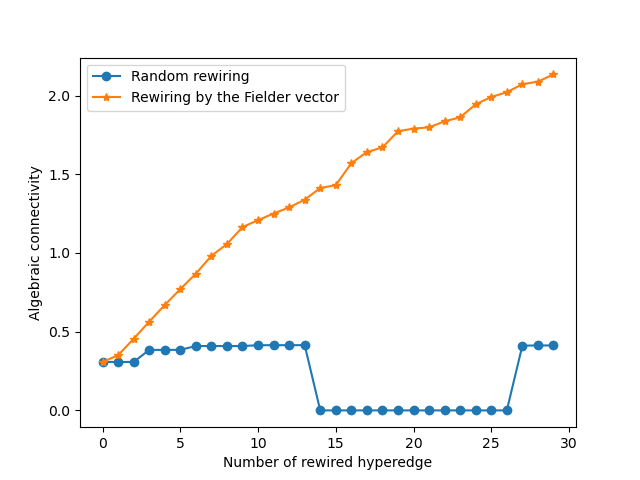
Refer to caption
Refer to caption
Figure 1: Results on the hyperedge rewiring problem.

The left-hand side is the result of the Contact-Primary-School dataset and the right side is on the Email-Enron dataset. The random rewiring may decrease the algebraic connectivity, as shown in the first case. If the only hyperedge between two parts is removed, the algebraic connectivity will decrease to 00 until a new hyperedge connecting these two parts is established. In comparison, our algorithm improve the algebraic connectivity efficiently.

For the hypergraph ARCCC problem, we firstly generate the weights in interval [0,1]01[0,1] and the cost for each hyperedge for the Email-Enron dataset. In the dataset, each hyperedge repeat several times, leading to a primal weight w¯i^subscript¯𝑤^𝑖\bar{w}_{\widehat{i}}\in\mathbb{N}. The adjusted weight wi^subscript𝑤^𝑖w_{\widehat{i}} and cost ci^subscript𝑐^𝑖c_{\widehat{i}} are based on this. The more a hyperedge is repeated, the higher it weighs and the less it costs. To be specific, we normalized it weight by

wi^=w¯i^maxi^{w¯i^}3.subscript𝑤^𝑖3subscript¯𝑤^𝑖subscript^𝑖subscript¯𝑤^𝑖w_{\widehat{i}}=\sqrt[3]{\frac{\bar{w}_{\widehat{i}}}{\max_{\widehat{i}}\{\bar{w}_{\widehat{i}}\}}}.

Its cost is computed as

ci^=maxi^{w¯i^}w¯i^.subscript𝑐^𝑖subscript^𝑖subscript¯𝑤^𝑖subscript¯𝑤^𝑖c_{\widehat{i}}=\sqrt{\frac{\max_{\widehat{i}}\{\bar{w}_{\widehat{i}}\}}{\bar{w}_{\widehat{i}}}}.

We use the square root and the cubic root to avoid a constant wi^ci^subscript𝑤^𝑖subscript𝑐^𝑖w_{\widehat{i}}c_{\widehat{i}}. If both are square root, we have wi^ci^=1subscript𝑤^𝑖subscript𝑐^𝑖1w_{\widehat{i}}c_{\widehat{i}}=1 for all i^^𝑖\widehat{i}. We use the cubic root on the weight so that wi^ci^>1subscript𝑤^𝑖subscript𝑐^𝑖1w_{\widehat{i}}c_{\widehat{i}}>1. For Ei^subscript𝐸^𝑖E_{\widehat{i}}\notin\mathcal{E}, we set ci^=2maxi^{wi^}subscript𝑐^𝑖2subscript^𝑖subscript𝑤^𝑖c_{\widehat{i}}=2\max_{\widehat{i}}\{w_{\widehat{i}}\}. The result is shown in Figure 2.

Refer to caption
Refer to caption
Figure 2: Results of the hypergraph ARCCC Problem on the Email-Enron dataset.

For the left-hand side, the cycle is the wi^subscript𝑤^𝑖w_{\widehat{i}}, where Ei^subscript𝐸^𝑖E_{\widehat{i}}\notin\mathcal{E} is omitted. The star is the solution of the hypergraph ARCCC problem after the following modification process. We omit the value that is less than 104superscript10410^{-4}, and the remains are greater than 102superscript10210^{-2}. There is no value located in this interval, which yields a sharp gap naturally. We normalized the weight by a linear map so that the maximum is 111. It is shown that the set of the remaining hyperedges is just \mathcal{E}, and the weights is quite near with the real weights. The right side is the relative error. We also make an example on the Contact-Primary-School dataset.
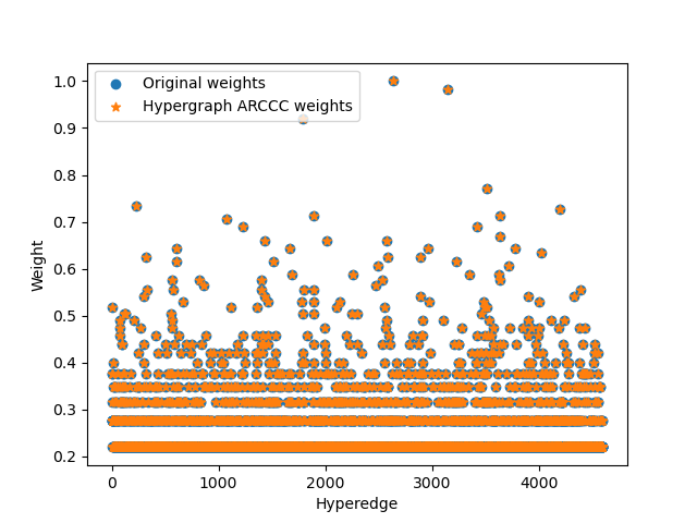
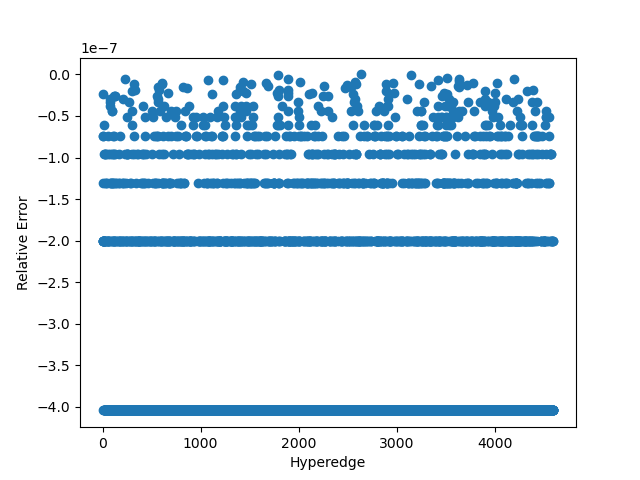
Refer to caption
Refer to caption
Figure 3: Results of the hypergraph ARCCC Problem on the Contact-Primary-School dataset.

The process of the following modification on the solution of the hypergraph ARCCC problem is the almost the same. The only different thing is that the gap is from 103superscript10310^{-3} to 101superscript10110^{-1}. It can be shown that the hypergraph ARCCC problem can capture the importance of each hyperedge efficiently.

6 Application in Dimensionality Reduction: Hypergraph Laplacian Eigenmap

The Laplacian eigenmap algorithm [7, 8] can be generalized to the hypergraph Laplacian eigenmap algorithm in our tensor product structure. The eigenmap step can also serve as a data preprocess step if the following clustering or classification algorithms use the linear distance rather than a kernel distance.

Algorithm 2 Hypergraph Laplacian Eigenmap

Input: Dataset {x1,,xn}n×psubscript𝑥1subscript𝑥𝑛superscript𝑛𝑝\{x_{1},\dots,x_{n}\}\in\mathbb{R}^{n\times p}.
Output: the dimension reduced dataset: {y1,,yn}n×qsubscript𝑦1subscript𝑦𝑛superscript𝑛𝑞\{y_{1},\dots,y_{n}\}\in\mathbb{R}^{n\times q}, qpmuch-less-than𝑞𝑝q\ll p.

1:Compute xixjnormsubscript𝑥𝑖subscript𝑥𝑗\|x_{i}-x_{j}\| for all ij𝑖𝑗i\neq j.
2:Find the m𝑚m nearest neighbors ni1,,nimsubscript𝑛𝑖1subscript𝑛𝑖𝑚n_{i1},\dots,n_{im} of xisubscript𝑥𝑖x_{i} for i=1,,n𝑖1𝑛i=1,\dots,n.
3:Construct an (m+1)𝑚1(m+1)-uniform hypergraph with ={Ei={ni1,,nim,xi}|i[n]}conditional-setsubscript𝐸𝑖subscript𝑛𝑖1subscript𝑛𝑖𝑚subscript𝑥𝑖𝑖delimited-[]𝑛\mathcal{E}=\left\{E_{i}=\{n_{i1},\dots,n_{im},x_{i}\}|i\in[n]\right\}.
4:Construct the Laplacian tensor and compute its eigenvalue and eigenvector.
5:Let {vi}i=1qsuperscriptsubscriptsubscript𝑣𝑖𝑖1𝑞\{v_{i}\}_{i=1}^{q} be the eigenvectors corresponding to the q𝑞q smallest non-zero eigenvalues, then {y1,,yn}={v1,,yq}subscript𝑦1subscript𝑦𝑛superscriptsubscript𝑣1subscript𝑦𝑞top\{y_{1},\dots,y_{n}\}=\{v_{1},\dots,y_{q}\}^{\top}.
6:return {y1,,yn}subscript𝑦1subscript𝑦𝑛\{y_{1},\dots,y_{n}\}.

We simply use the Laplacian tensor to compute the eigenvector rather than the normalized Laplacian matrix in the classic graph Laplacian eigenmap algorithm in [7, 8]. We applied the original Laplacian eigenmap algorithm and our hypergraph Laplacian eigenmap algorithm and then perform a standard K𝐾K-means clustering algorithm after the dimensionality reduction. The performance is further measured by the normalized mutual information and the adjusted Rand score. Both the K𝐾K-means algorithm and the two measures are from the package Scikit-learn in python. Before dimensionality reduction, a normalization step for each attribute of the dataset is performed. All the datasets are from KEEL dataset repository. The result is shown below. The Breast Cancer Wisconsin (Diagnostic) dataset has 33 attributes, we choose m=7𝑚7m=7 nearest neighbors of each vertex, leading to an 888-uniform hypergraph. In the graph Laplacian eigenmap, this means each vertex is connected to 777 nearest vertices. We use the 01010-1 weight rather than the heat kernel weight to avoid the choice of the heat hyperparameter t𝑡t in [7, 8].

We use HLE as the abbreviation for the hypergraph Laplacian eigenmap, and GLE for the graph Laplacian eigenmap. The horizontal coordinate is the reduced dimension.
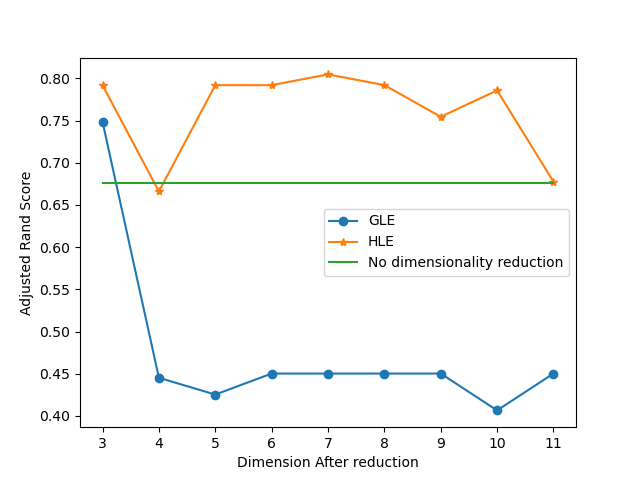
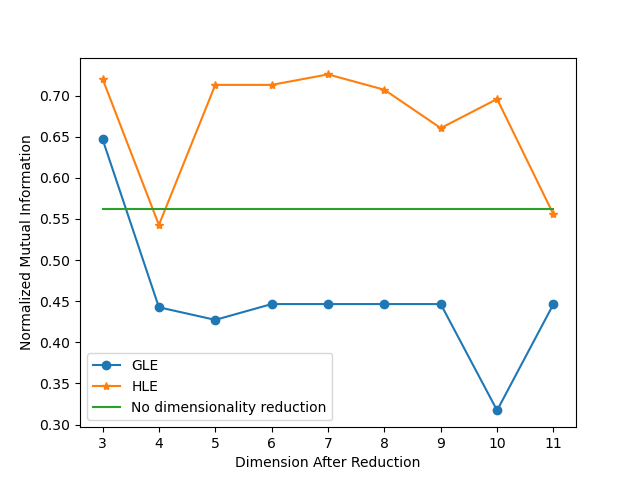
Refer to caption
Refer to caption
Figure 4: Results on the Breast Cancer Wisconsin (Diagnostic) dataset.

The green horizontal line in the figures is the result with no dimensionality reduction. We simply perform the K𝐾K-means algorithm on the normalized datasets and use this result as a baseline. Our hypergraph Laplacian eigenmap algorithm has better performance and better stability than the classic Laplacian eigenmap algorithm. The same result happens on the Dermatology dataset and the Movement of Libras dataset, which are shown in Figure 5 and 6.
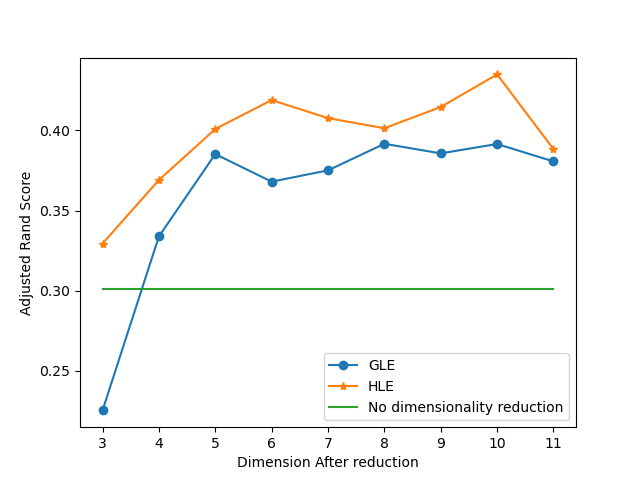
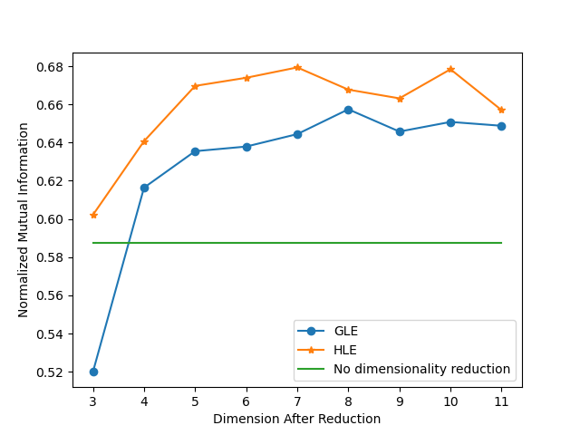
Refer to caption
Refer to caption
Figure 5: Results on the Movement of Libras dataset.
Refer to caption
Refer to caption
Figure 6: Results on the Dermatology dataset.

In the third section, we mentioned that our structure is the same as the clique reduction technique in some cases. This means each hyperedge contains more edges. A hyperedge containing (m+1)𝑚1(m+1) vertices actually contains 12m(m+1)12𝑚𝑚1\frac{1}{2}m(m+1) edges in the view of the clique reduction. On the other hand, in our algorithm we remove the normalized item xDx=Isuperscript𝑥top𝐷𝑥𝐼x^{\top}Dx=I. To show that the improvement is neither due to the removal of the normalized term, nor due to the increase of edges, there is a detailed comparison.

To figure out the influence of increasing edges, we firstly increase the number of nearest neighbors in the graph Laplacian eigenmap algorithm to 12m(m+1)=2812𝑚𝑚128\frac{1}{2}m(m+1)=28.

Refer to caption
Refer to caption
Figure 7: Influence of more edges on the Breast Cancer Wisconsin (Diagnostic) dataset.

It can be seen that increasing the number of edges does not always improve the performance. This can also be seen in the results on the other two datasets, especially on the Movement of Libras dataset.

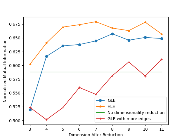
Refer to caption
Refer to caption
Figure 8: Influence of more edges on Movement of Libras dataset.
Refer to caption
Refer to caption
Figure 9: Influence of more edges on the Dermatology dataset.

We also need to clarify the influence of the normalization item. In the following experiments we remove the normalization item. We also make an example of these two factors to figure out whether the improvement is due to a combined action.
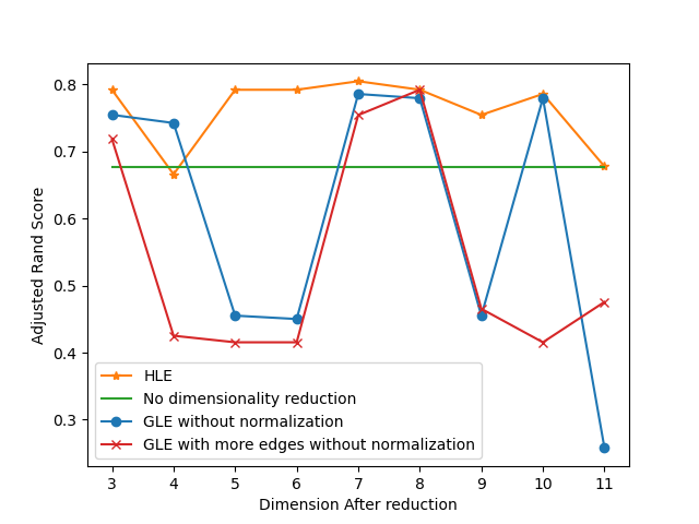
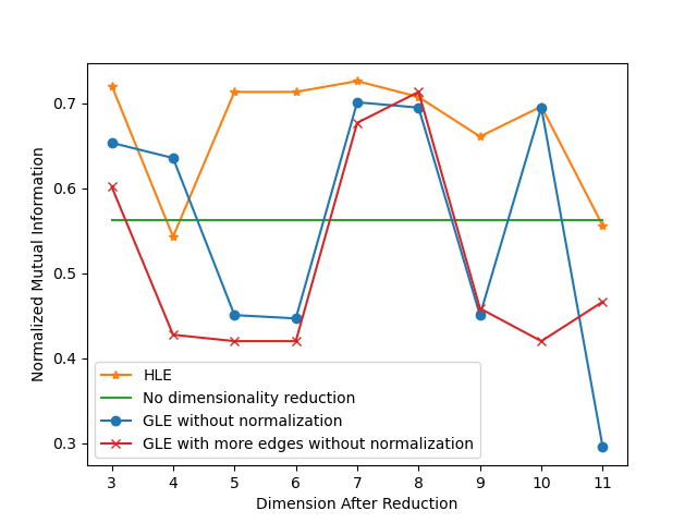
Refer to caption
Refer to caption
Figure 10: Influence of the normalization term on the Breast Cancer Wisconsin (Diagnostic) dataset.
Refer to caption
Refer to caption
Figure 11: Influence of the normalization term on the Movement of Libras dataset.
Refer to caption
Refer to caption
Figure 12: Influence of the normalization term on the Dermatology dataset.

It can be seen that removing the normalization item is not so good as the hypergraph Laplacian eigenmap algorithm. Moreover, if we increase the number of edges in the graph Laplacian eigenmap algorithms without the normalization term, the result is still not so good as our hypergraph Laplacian eigenmap algorithm. This shows the improvement is not due to either one of these two factors, or a combined action. In conclusion, our structure provides a hypergraph Laplacian eigenmap algorithm, and have better performance than the classic graph Laplacian eigenmap algorithm.

Acknowledgements

The authors would like to thank the handling editor and the referee for their detailed comments.

References

  • [1] S. Agarwal, K. Branson, and S. Belongie, Higher order learning with graphs, in Proceedings of the 23rd international conference on Machine learning, 2006, pp. 17–24.
  • [2] E. Albert, Die grundlage der allgemeinen relativitätstheorie, Annalen der Physik., 49 (1916), pp. 769–822.
  • [3] M. M. Asadi, M. Khosravi, A. G. Aghdam, and S. Blouin, Generalized algebraic connectivity for asymmetric networks, in 2016 American Control Conference (ACC), 2016, pp. 5531–5536.
  • [4] G. Ausiello, P. G. Franciosa, and D. Frigioni, Directed hypergraphs: Problems, algorithmic results, and a novel decremental approach, in Italian conference on theoretical computer science, Springer, 2001, pp. 312–328.
  • [5] G. Ausiello and L. Laura, Directed hypergraphs: Introduction and fundamental algorithms—a survey, Theoretical Computer Science, 658 (2016), pp. 293–306.
  • [6] R. B. Bapat, Graphs and Matrices, London: Springer; New Delhi: Hindustan Book Agency, 2nd ed. ed., 2014.
  • [7] M. Belkin and P. Niyogi, Laplacian eigenmaps and spectral techniques for embedding and clustering, Advances in Neural Information Processing Systems, 14 (2001), pp. 585–591.
  • [8] M. Belkin and P. Niyogi, Laplacian eigenmaps for dimensionality reduction and data representation, Neural computation, 15 (2003), pp. 1373–1396.
  • [9] A. R. Benson, R. Abebe, M. T. Schaub, A. Jadbabaie, and J. Kleinberg, Simplicial closure and higher-order link prediction, Proceedings of the National Academy of Sciences, 115 (2018), pp. E11221–E11230.
  • [10] M. Brazell, N. Li, C. Navasca, and C. Tamon, Solving multilinear systems via tensor inversion, SIAM Journal on Matrix Analysis and Applications, 34 (2013), pp. 542–570.
  • [11] R. Cambini, G. Gallo, and M. G. Scutellá, Flows on hypergraphs, Mathematical Programming, 78 (1997), pp. 195–217.
  • [12] M. Che and Y. Wei, Theory and Computation of Complex Tensors and its Applications, Singapore: Springer, 2020.
  • [13] C. Chen, Explicit solutions and stability properties of homogeneous polynomial dynamical systems, IEEE Transactions on Automatic Control, 68 (2023), pp. 4962–4969.
  • [14] C. Chen, A. Surana, A. Bloch, and I. Rajapakse, Multilinear time invariant system theory, in 2019 Proceedings of the Conference on Control and its Applications, SIAM, 2019, pp. 118–125.
  • [15] C. Chen, A. Surana, A. M. Bloch, and I. Rajapakse, Multilinear control systems theory, SIAM Journal on Control and Optimization, 59 (2021), pp. 749–776.
  • [16] K.-F. Cheung and M. G. Bell, Improving connectivity of compromised digital networks via algebraic connectivity maximisation, European Journal of Operational Research, 294 (2021), pp. 353–364.
  • [17] J. Cooper and A. Dutle, Spectra of uniform hypergraphs, Linear Algebra and its Applications, 436 (2012), pp. 3268–3292.
  • [18] K. Feng and W.-C. W. Li, Spectra of hypergraphs and applications, Journal of Number Theory, 60 (1996), pp. 1–22.
  • [19] M. Fiedler, Algebraic connectivity of graphs, Czechoslovak Mathematical Journal, 23 (1973), pp. 298–305.
  • [20] G. Gallo, G. Longo, S. Pallottino, and N. Sang, Directed hypergraphs and applications, Discrete Applied Mathematics, 42 (1993), pp. 177–201.
  • [21] A. Ghosh and S. Boyd, Growing well-connected graphs, in Proceedings of the 45th IEEE Conference on Decision and Control, IEEE, 2006, pp. 6605–6611.
  • [22] C. Godsil and G. Royle, Algebraic graph theory, vol. 207 of Graduate Texts in Mathematics, Springer-Verlag, New York, 2001.
  • [23] A. Hagberg and D. A. Schult, Rewiring networks for synchronization, Chaos: An Interdisciplinary Journal of Nonlinear Science, 18 (2008), p. 037105.
  • [24] S. Hu and L. Qi, Algebraic connectivity of an even uniform hypergraph, Journal of Combinatorial Optimization, 24 (2012), pp. 564–579.
  • [25] S. Kar and J. M. Moura, Consensus based detection in sensor networks: Topology optimization under practical constraints, Proc. 1st Intl. Wrkshp. Inform. Theory Sensor Networks, 13 (2007), p. 31.
  • [26]  , Sensor networks with random links: Topology design for distributed consensus, IEEE Transactions on Signal Processing, 56 (2008), pp. 3315–3326.
  • [27] Y. Kim, Bisection algorithm of increasing algebraic connectivity by adding an edge, IEEE Transactions on Automatic Control, 55 (2010), pp. 170–174.
  • [28] T. Kolokolnikov, Maximizing algebraic connectivity for certain families of graphs, Linear Algebra and its Applications, 471 (2015), pp. 122–140.
  • [29] E. L. Lawler, Cutsets and partitions of hypergraphs, Networks, 3 (1973), pp. 275–285.
  • [30] H. Li, J.-Y. Shao, and L. Qi, The extremal spectral radii of k𝑘k-uniform supertrees, Journal of Combinatorial Optimization, 32 (2016), pp. 741–764.
  • [31] W. Li, J. Cooper, and A. Chang, Analytic connectivity of k-uniform hypergraphs, Linear and Multilinear Algebra, 65 (2017), pp. 1247–1259.
  • [32] S. Mackay, C. Ponce, S. Osborn, and M. McGarry, Finding diverse ways to improve algebraic connectivity through multi-start optimization, Journal of Complex Networks, 9 (2021), p. cnab005.
  • [33] Y. Miao, Y. Wei, and Z. Chen, Fourth-order tensor Riccati equations with the Einstein product, Linear and Multilinear Algebra, 70 (2022), pp. 1831–1853.
  • [34] H. Nagarajan, S. Rathinam, and S. Darbha, On maximizing algebraic connectivity of networks for various engineering applications, in 2015 European Control Conference (ECC), IEEE, 2015, pp. 1626–1632.
  • [35] K. Ogiwara, T. Fukami, and N. Takahashi, Maximizing algebraic connectivity in the space of graphs with a fixed number of vertices and edges, IEEE Transactions on Control of Network Systems, 4 (2017), pp. 359–368.
  • [36] L. Qi and Z. Luo, Tensor Analysis. Spectral Theory and Special Tensors, Philadelphia, PA: Society for Industrial and Applied Mathematics, 2017.
  • [37] L. Qi, J. Y. Shao, and Q. Wang, Regular uniform hypergraphs, s𝑠s-cycles, s𝑠s-paths and their largest laplacian h-eigenvalues, Linear Algebra and its Applications, 443 (2014), pp. 215–227.
  • [38] Y. Qi, Z. Zhang, Y. Yi, and H. Li, Consensus in self-similar hierarchical graphs and sierpiński graphs: Convergence speed, delay robustness, and coherence, IEEE transactions on cybernetics, 49 (2018), pp. 592–603.
  • [39] G. Sudhakara, V. Madhusudanan, and K. Arathi Bhat, On Products of Graph Matrices, Springer Nature Singapore, Singapore, 2023, pp. 337–377.
  • [40] L. Sun, B. Zheng, C. Bu, and Y. Wei, Moore-Penrose inverse of tensors via Einstein product, Linear and Multilinear Algebra, 64 (2016), pp. 686–698.
  • [41] A. Sydney, C. Scoglio, and D. Gruenbacher, Optimizing algebraic connectivity by edge rewiring, Applied Mathematics and computation, 219 (2013), pp. 5465–5479.
  • [42] N. Veldt, A. R. Benson, and J. Kleinberg, Hypergraph cuts with general splitting functions, SIAM Review, 64 (2022), pp. 650–685.
  • [43] N. Veldt, A. R. Benson, and J. Kleinberg, Hypergraph cuts with general splitting functions, SIAM Review, 64 (2022), pp. 650–685.
  • [44] A. P. Volpentesta, Hypernetworks in a directed hypergraph, European Journal of Operational Research, 188 (2008), pp. 390–405.
  • [45] J.-C. Wan, Y. Wang, and F.-T. Hu, Spectra of weighted uniform hypertrees, The Electronic Journal of Combinatorics, (2022), pp. P2–40.
  • [46] Y. Wang and Y. Wei, Generalized eigenvalue for even order tensors via einstein product and its applications in multilinear control systems, Computational and Applied Mathematics, 41 (2022). article 419.
  • [47] P. Wei, L. Chen, and D. Sun, Algebraic connectivity maximization of an air transportation network: The flight routes’ addition/deletion problem, Transportation Research Part E: Logistics and Transportation Review, 61 (2014), pp. 13–27.
  • [48] P. Wei, G. Spiers, and D. Sun, Algebraic connectivity maximization for air transportation networks, IEEE Transactions on Intelligent Transportation Systems, 15 (2013), pp. 685–698.
  • [49] Y. Wei and W. Ding, Theory and Computation of Tensors. Multi-dimensional Arrays, Amsterdam: Elsevier/Academic Press, 2016.
  • [50] C. W. Wu, Algebraic connectivity of directed graphs, Linear and Multilinear Algebra, 53 (2005), pp. 203–223.
  • [51] G. Wu and Y. Wei, Relationship between the characteristic polynomial and the spectrum of a diagonalizable matrix and those of its low-rank update, Linear and Multilinear Algebra, 60 (2012), pp. 967–978.
  • [52] J. Xie and L. Qi, Spectral directed hypergraph theory via tensors, Linear and Multilinear Algebra, 64 (2016), pp. 780–794.