Estimating the Uncertainty of Cosmological First Order Phase Transitions with Numerical Simulations

Abstract

In order to study the validity of analytical formulas used in the calculation of characteristic physical quantities related to vacuum bubbles, we conduct several numerical simulations of bubble kinematics in the context of cosmological first-order phase transitions to determine potentially existing systematic uncertainties. By comparing with the analytical results, we obtain the following observations: (1) For the total number of bubbles, there is a $10\%$ discrepancy between the values from simulations and from analytical prediction; (2) For the false vacuum fraction, the difference between the results from simulations and from analytical prediction is small, which, however, plays a crucial role in explaining the discrepancy observed in the total number of bubbles; (3) The bubble lifetime distribution obtained from the simulations deviates from the exponential distribution and is not obviously influenced by different nucleation rates; (4) These differences propagate into the final gravitational waves spectra, which we calculate with the sound shell model for the usually dominant contribution from sound waves, and find that the bubble number deviation enhances the peak value in the gravitational wave spectra, while the deviation in the lifetime distribution suppresses the peak value.

I Introduction

With the first direct detection of gravitational waves induced by the merger of binary black holes Abbott et al. (2016), the era of gravitational wave observations has arrived. One of the next important goals is to search for stochastic gravitational waves from the cosmic first-order phase transition and probe the possible new physics beyond the standard model Weir (2018); Mazumdar and White (2018); Bertone et al. (2020). To the end, LIGO and Virgo have already taken the first step Abbott et al. (2017); Scientific et al. (2019) and many space-based detectors have been proposed, such as the Laser Interferometer Space Antenna (LISA) Amaro-Seoane et al. (2017), Taiji Gong et al. (2015) and Tianqin Luo et al. (2016). These detectors are expected to be completed in a decade or so and start to search for low-frequency gravitational waves induced at the electroweak scale Athron et al. (2023a); Han et al. (2021); Guo et al. (2021); Yang et al. (2023); Xiao et al. (2023); Balázs et al. (2023); Vaskonen (2017); Beniwal et al. (2019); Kang et al. (2018); Chala et al. (2018); Alves et al. (2020, 2019); Chao et al. (2017).

In terms of phenomenological analysis, it is well known that the source of phase transition gravitational wave comes from three parts: bubble collision, sound wave, and turbulence. The contribution of bubble collision to observable gravitational waves can be well described by the envelope approximation Kosowsky et al. (1992); Kosowsky and Turner (1993) and the corresponding analytical formula has already been derived Jinno and Takimoto (2017). Furthermore, lattice simulation results can provide more information than the envelope approximation and have yielded the standard spectral formulas that are widely used Hindmarsh et al. (2015, 2017). The lattice results show that the contribution of sound waves is much larger than the collisions Hindmarsh et al. (2014, 2015, 2017). To describe it, many simplified models have been developed, such as the sound shell model Hindmarsh (2018); Hindmarsh and Hijazi (2019) and the bulk flow model Jinno and Takimoto (2019); Konstandin (2018) as well as their extensions Cai et al. (2023a), in which the power laws can be accurately reproduced. In contrast to the first two parts, the early understanding of turbulence was almost entirely derived from theoretical calculations Kosowsky et al. (2002); Dolgov et al. (2002); Caprini et al. (2009), whereas recently numerical simulations have started to be performed Yang and Bian (2022); Di et al. (2021).

To keep up with advances in experiments, there is increasing attention being paid to the study of uncertainties in the calculations mentioned above, such as the uncertainties in the effective potential Croon et al. (2021); Athron et al. (2023b) and in the calculation of bounce actions Andreassen et al. (2017); Dunne and Min (2005) and nucleation rate Ekstedt (2022). In this work, we will address the uncertainties involved in estimating the pre-factor in the nucleation rate and calculating the false vacuum fraction.

The uncertainty of the pre-factor arises from the determinant related to the potential, which is model-dependent and difficult to obtain with high precision. It is typically approximately estimated using one of three approaches: (1) taking the fourth power of the critical temperature Hindmarsh and Hijazi (2019); Guth and Weinberg (1981), (2) taking the fourth power of temperature Enqvist et al. (1992); Guo et al. (2021); Han et al. (2021); Alves et al. (2019); Chao et al. (2017), and (3) taking the fourth power of temperature while incorporating the bounce action Athron et al. (2023c); Cai et al. (2017). The use of different pre-factors can lead to different rates of nucleation, resulting in different kinematic processes in both analytical calculations and numerical simulations. Another widely used approximation is the simplified formula that describes the fraction of false vacuum in the early universe. It was originally derived by Guth et al Guth and Weinberg (1981), where the overlapped regions of bubbles and phantom bubbles are double counted. As a result, the false vacuum fraction may be underestimated.

Both the nucleation rate and the false vacuum fraction are essential factors in describing bubble kinematics. In the sound shell model, many statistical measures related to gravitational waves are dependent on these factors, such as the bubble mean separation and the bubble lifetime distribution. Therefore, any variation in these factors may potentially affect the predicted gravitational wave spectra. It is interesting to adopt the semi-analytical and semi-simulated approach to find out how much difference on the gravitational wave spectra can arise from choosing different pre-factor modes and the theoretical framework for the false vacuum fraction.

The aim of this work is to conduct a bubble simulation based on three different nucleation rates and compare the simulated values with the analytical results for the false vacuum fraction, the total bubble number, and the bubble lifetime distribution to obtain insights into the uncertainties. The paper is structured as follows: in section II, we present the theoretical framework for the relevant quantities; section III describes the simulation details; in section IV, we compare the simulation results with the theoretical predictions; and finally, we conclude in section V.

II Physical quantities in bubble kinematics

During the early universe, bubbles of true vacuum formed within the false vacuum environment. The nucleation rate, i.e., the number of bubbles nucleated per unit time per unit volume, can be roughly estimated as Linde (1983)

$$\Gamma\sim Ae^{-S_{3}/T},$$ (1)

where $A$ is a pre-factor and $S_{3}$ is the three-dimensional Euclidean action given by

$$S_{3}=4\pi\int^{+\infty}_{0}r^{2}{\rm d}r~{}\left[\frac{1}{2}\left(\frac{\partial\phi}{\partial r}\right)^{2}+V(\phi,T)\right].$$ (2)

The bubble configuration $\phi(r)$ in the integral is fixed from the corresponding Euclidean equation of motion

$$\frac{{\rm d}^{2}\phi}{{\rm d}r^{2}}+\frac{2}{r}\frac{{\rm d}\phi}{{\rm d}r}=\frac{\partial V(\phi,T)}{\partial\phi},$$ (3)

subjected to the boundary conditions (see Refs. Rubakov (2009); Linde (1983) for details)

$$\lim\limits_{r\to\infty}\phi(r)=0,~{}~{}{\rm d}\phi/{\rm d}r|_{r=0}=0.$$ (4)

The pre-factor is proportional to the fourth power of temperature on dimensional grounds, and more precisely its specific value is given by Linde (1983)

$$A=T\left(\frac{S_{3}}{2\pi T}\right)^{\frac{3}{2}}\frac{{\rm det}^{\prime}\left[-\Delta+V^{\prime\prime}(\phi,T)\right]}{{\rm det}\left[-\Delta+V^{\prime\prime}(0,T)\right]},$$ (5)

where $\rm{det}^{\prime}$ implies that three zero eigenvalues of the operator $-\Delta+V^{\prime\prime}(\phi,T)$ are to be omitted when computing the determinant. Its precise determination requires integrating out fluctuations around the bounce solution, as demonstrated in Refs.Andreassen et al. (2017); Dunne and Min (2005). For simplification, three approximate estimations have been proposed and are commonly used:

1. $A=T_{\rm c}^{4}$, where $T_{\rm c}$ is the critical temperature,

2. $A=T^{4}$ ,

3. $A=T^{4}(\frac{S_{3}}{2\pi T})^{\frac{3}{2}}$.

In the following, we refer them as pre-factor1, pre-factor2 and pre-factor3, respectively. These modes will yield different nucleation rates and, consequently, affect the bubble kinematics later on.

After nucleation, the bubbles may expand and merge until the entire universe is filled with true vacuum. The percolation temperature, denoted as $T_{\rm p}$, is defined as the temperature at which the false vacuum occupies 70% of the volume of the universe. To account for the remained fraction of space in the false vacuum, we follow Guth and Weinberg’s procedure Guth and Weinberg (1981) and consider a space containing randomly placed spheres (including overlapped and nested spheres). We then calculate the probability that a given point is not contained within any existing sphere.

Denoting $\rho(V)dV$ as the density of spheres with volume between $V$ and $V+dV$, $V_{\rm s}$ as the volume of the entire space, and $g(V_{1},V_{2})$ as the probability that a given point is not contained in any existing sphere with volume between $V_{1}$ and $V_{2}$, we can derive the following equation,

$$g(V_{1},V_{2}+dV_{2})= g(V_{1},V_{2})g(V_{2},V_{2}+dV_{2})$$ (6)

$$= g(V_{1},V_{2})\frac{V_{\rm s}-V_{\rm s}\rho(V_{2})dV_{2}V_{2}}{V_{\rm s}}$$

$$= g(V_{1},V_{2})(1-\rho(V_{2})dV_{2}V_{2}),$$

which then leads to a differential equation for $g$:

$$\frac{dg(V_{1},V_{2})}{dV_{2}}=-\rho(V_{2})g(V_{1},V_{2})V_{2}.$$ (7)

The solution of this equation is

$$g(V_{1},V_{2})={\rm{exp}}\left[-\int_{V_{1}}^{V_{2}}dV\rho(V)V\right].$$ (8)

In particular, the probability that the given point is not contained within any existing sphere is

$$g(0,\infty)={\rm{exp}}\left[-\int_{0}^{\infty}dV\rho(V)V\right].$$ (9)

Returning to the picture of the first-order transition and taking into account the fact that the bubbles forming at the same time have the same volume, we can substitute $\rho(V)dV$ with $\Gamma(t)dt$. Therefore, in a flat spacetime, the fraction of false vacuum can be approximated as

$$h(t)\equiv g(t_{\rm c},t)={\rm{exp}}\left[-\int^{t}_{t_{\rm c}}\Gamma(t^{\prime})V(t^{\prime},t)dt^{\prime}\right],$$ (10)

where $V(t^{\prime},t)=\frac{4\pi}{3}[\int^{t}_{t^{\prime}}v_{\rm w}(\tau)d\tau]^{3}$ and $v_{\rm w}$ is the bubble wall velocity. It is clear from the above discussion that the overlapped regions and nested spheres are double-counted in this procedure. Furthermore, Eq.(6) potentially implies that the total volume of space $V_{\rm s}$ is infinite, so that the total volume of the overlapped spheres will not exceed it. However, in reality, the volume of the universe is finite, and some finite-volume effects may arise when calculating $h(t)$ within a finite region.

Thus, Eq.(10) does not precisely characterize the phase transition picture, and as a result, the estimated start and end time of the transition may be inaccurate, which could impact the predicted gravitational spectra. Obtaining a closed-form solution for the false vacuum fraction is difficult, and therefore, Monte Carlo simulations are needed. An alternative approach that is more accurate and efficient but complex is to use Voronoi diagrams in Laguerre geometry Imai et al. (1985).

Eq. (10) can be simplified even further by expanding the action in the vicinity of the time $t_{f}$, at which $h(t_{f})=1/e$  Enqvist et al. (1992):

$$h(t)={\rm{exp}}\left[-e^{\beta(t-t_{f})}\right],$$ (11)

where $\beta=-d{\rm{ln}}\Gamma/dt$. We now have two key ingredients, i.e., the false vaccum fraction and the nucleation rate. It is worth noting that bubbles can only be generated in the false vacuum region. As a result, the total number of nucleated bubbles before time $t$ within the volume $V_{\rm s}$ can be expressed as Enqvist et al. (1992)

$$N_{\text{tot}}(t)=\int_{t_{\rm c}}^{t}V_{\rm s}\Gamma(t^{\prime})h(t^{\prime})dt^{\prime},$$ (12)

where $t_{\rm c}$ is the evolution time corresponding to the critical temperature $T_{\rm c}$. The mean separation between bubbles can be defined as

$$R^{*}=\left(\frac{V_{\rm s}}{N_{\rm tot}}\right)^{\frac{1}{3}}.$$ (13)

Figure 1: The schematic diagram for calculating the bubble lifetime distribution. At time $t_{1}$, three bubbles are generated randomly. The two blue bubbles merge at $t_{2}$, and contact the red bubble at $t_{3}$. If the distance between the red bubble and the blue phase boundary is $L$, then at time $t_{2}+\bar{t}=t_{2}+L/v_{\rm w}$, the red bubble nucleation site will be occupied. At this time, the radius of the red bubble is $L$ and the lifetime is $\bar{t}=L/v_{\rm w}$.

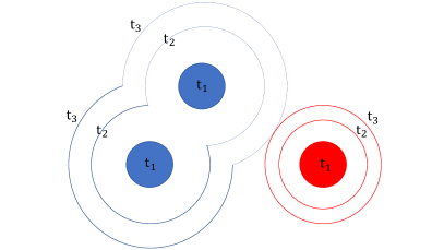
Another useful statistical measure is the bubble lifetime distribution, which characterizes the lifetimes for all the bubbles that were formed and subsequently destroyed during the phase transition process Hindmarsh and Hijazi (2019); Hijazi (2022). A bubble is considered as being destroyed when the nucleation site is first occupied by the true vacuum space, as illustrated in Fig. 1. To analyze the bubble lifetime distribution, we first define the unbroken bubble wall area per unit volume $S$ as Hindmarsh and Hijazi (2019); Guo et al. (2021)

$$\frac{dV_{\rm false}}{V_{\rm s}}=-SdR=-Sv_{\rm w}dt.$$ (14)

The number of bubbles with a radius of $R$ at the time of their destruction, which occurs after a time $\bar{t}=R/v_{\rm w}$, is given by the following expression (see Fig.1 for more details):

$$d^{2}n=S(t^{\prime}+R/v_{\rm w})\Gamma(t^{\prime})dRdt^{\prime}.$$ (15)

By integrating this expression, we can obtain the bubble size distribution,

$$\frac{dn}{dR}=\int_{t_{\rm c}}^{\infty}S(t^{\prime}+R/v_{\rm w})\Gamma(t^{\prime})dt^{\prime}.$$ (16)

The fraction of bubbles with lifetime in the range $\left[\bar{t},\bar{t}+d\bar{t}\right]$ is

$$f=\frac{dn}{dR}\frac{dR}{d\bar{t}}=v_{\rm w}\frac{dn}{dR}.$$ (17)

Adopting Eq.(11), we can express the normalized bubble lifetime distribution $\nu$ simply as  Hindmarsh and Hijazi (2019)

$$\nu(\beta\bar{t})=e^{-\beta\bar{t}}.$$ (18)

Assuming that the bubble will attain a steady velocity as a result of friction, the velocity profile $v_{\rm plasma}$ and enthalpy profile $w_{\rm plasma}$ of the plasma surrounding a single bubble can be calculated by using the hydrodynamics within a simplified bag model Espinosa et al. (2010). Those self-similar profiles become the initial condition for freely propagating, after some forced propagating period Cai et al. (2023b). In the sound shell model, the total velocity profile is assumed to be a superposition of these velocity perturbations Hindmarsh (2018); Hindmarsh and Hijazi (2019)

$$v_{\rm plasma}^{\rm tot}=\sum_{i=1}^{\rm{N_{tot}}}v_{\rm plasma}^{i}.$$ (19)

Then the velocity power spectrum can be derived

$$\mathcal{P}_{v}(q)=\frac{2}{2\pi^{2}(\beta R^{*})^{3}}(\frac{q}{\beta})^{3}\int\nu(\tilde{T})\tilde{T}^{6}\left|A(\tilde{T}q/\beta)\right|^{2}d\tilde{T},$$ (20)

where

$$A(z) =0.5(f^{\prime}(z)+ic_{s}l(z)),$$ (21)

$$f(z) =\frac{4\pi}{z}\int v_{\rm plasma}(\xi)\sin(z\xi)d\xi,$$

$$l(z) =\frac{4\pi}{z}\int\frac{e_{\rm plasma}(\xi)-\bar{e}}{\bar{w}}\xi\sin(z\xi)d\xi,$$

and $\bar{e},\bar{w}$ are the mean energy and enthalpy densities, respectively. The gravitational wave power spectrum before redshift $\mathcal{P}_{\text{GW}}$ is defined as the contribution to the density fraction in gravitational waves per logarithmic wave number interval. With the help of $\mathcal{P}_{v}$, the gravitational wave power spectrum generated by the stationary velocity power spectrum with a lifetime $\tau_{v}$ can be expressed as

$$\mathcal{P}_{\text{GW}}=3(\Gamma_{w}\bar{U}_{f}^{2})^{2}(H\tau_{v})(HL_{f})\frac{(qL_{f})^{3}}{2\pi^{2}}\tilde{P}(qR^{*}),$$ (22)

where $\Gamma_{w}$ is the ratio of enthalpy to energy, $\bar{U}_{f}$ is the RMS fluid velocity, $L_{f}$ is the length scale in the velocity field and

$$\tilde{P}(y)=\frac{1}{4\pi yc_{\rm s}}\left(\frac{1-c_{s}^{2}}{c_{s}^{2}}\right)^{2}$$

$$\times\int^{z_{+}}_{z{-}}\frac{dz}{z}\frac{(z-z_{+})^{2}(z-z_{-})^{2}}{z_{+}+z_{-}-z}\bar{P}_{v}(z)\bar{P}_{v}(z_{+}+z_{-}-z),$$

with $\bar{P}_{v}=\frac{\pi^{2}\mathcal{P}_{v}}{q^{3}{R^{*}}^{3}\bar{U}_{f}^{2}}$ and $z_{\pm}=y(1\pm c_{\rm s})/2c_{\rm s}$. After redshifting, the power spectrum today at frequency $f$ is Gowling and Hindmarsh (2021)

$$\Omega_{\text{GW}}h^{2}=3.57\times 10^{-5}\left(\frac{100}{g_{*}}\right)^{\frac{1}{3}}\Sigma(v_{\rm w},\alpha)\mathcal{P}_{\text{GW}}(qR^{*}(f)),$$ (24)

where $g_{*}$ is the number of relativistic degrees of freedom, $\Sigma(v_{\rm w},\alpha)$ is a suppression factor found from recent numerical simulations for strong phase transitions Cutting et al. (2020) and

$$f=2.6\times 10^{-6}\frac{qR^{*}}{HR^{*}}\left(\frac{T}{100\,\text{GeV}}\right)\left(\frac{g_{*}}{100}\right)^{\frac{1}{6}}\mathrm{Hz}.$$ (25)

In this paper, we set $\Sigma$ as one because it is a constant and does not affect the uncertainty.

III Simulation framework and toy quartic model

To simulate the random generation of bubbles according to Eq.(1), we follow the method proposed by J. Ignatius et al. Enqvist et al. (1992)

• The phase transition begins when the temperature falls below the critical temperature, so the starting time is set to $t_{1}=t_{\rm c}$, at the critical temperature $T=T_{\rm c}$. The probability that no bubbles are nucleated in the volume $V_{\rm s}$ during the time interval $t_{1}\leq t\leq t_{2}$ can be expressed as

  $$p(t_{2},t_{1})={\rm{exp}}\left(-\int_{t_{1}}^{t_{2}}V_{\rm s}\Gamma dt\right).$$ (26)

• The start time of next bubble nucleated is $t_{2}$, which is obtained by solving

  $$p(t_{2},t_{1})=r,$$ (27)

  where $r$ is a uniformly distributed random number between 0 and 1.

• Choose a random location for the bubble within $V_{\rm s}$. If the location falls within a previously generated bubble at $t_{2}$, reject the bubble and return to step (1).

• Increase the radius of all the bubbles individually by

  $$R(t)=\int_{t_{birth}}^{t}v_{\rm w}(\tau)d\tau.$$ (28)

• Replace $t_{1}$ with $t_{2}$ and return to step (1) until the bubbles fill the entire space.

As is typical in simulations, we adopt the following effective potential

$$V(\phi,T)= \frac{1}{2}M^{2}(T)\phi^{2}-\frac{1}{3}\delta(T)\phi^{3}+\frac{1}{4}\lambda\phi^{4}$$ (29)

$$= \frac{1}{2}\gamma(T^{2}-T_{0}^{2})\phi^{2}-\frac{1}{3}\alpha T\phi^{3}+\frac{1}{4}\lambda\phi^{4},$$

where $T_{0}$, $\gamma$, $\alpha$, $\lambda$ are adjustable parameters, and here are set to be 75 GeV, 0.2, 0.3, 0.2, respectively. This expression can be deduced from the high temperature expansion for standard model extensions if no extra scalar field is added.

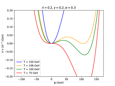
In the early universe, when the temperature is higher than a threshold $T_{0}$, i.e. $T\geq T_{0}$, the potential has a minimum at $\phi=0$ and $V(\phi=0,T)=0$, indicating that the symmetry is restored. The minimum corresponding to symmetry-broken vacuum appears at low temperature, with an expectation value of

$$v(T)=\frac{\alpha T}{2\lambda}\left(1+\sqrt{1-\frac{4\lambda M(T)^{2}}{\delta^{2}}}\right).$$ (30)

The critical temperature, at which the two minimums have the same free energy, can be determined as

$$T_{\rm c}=\sqrt{\frac{T_{0}^{2}}{1-\frac{2\alpha^{2}}{9\lambda\gamma}}}.$$ (31)

When the temperature decreases below $T_{0}$, the origin becomes a maximum instead of a minimum, and there is no phase transition but rather spinodal decomposition. An example of the variation of the effective potential with temperature is displayed in Fig. 2.

Figure 2: The scaled effective potential for the effective model in Eq.(29) varied with temperature when $\lambda$ = 0.2, $\gamma$ = 0.2, $\alpha$ = 0.3. ${T_{\rm c}}\approx 106$ GeV is the critical temperature at which the two minimums have the same potential. ${T_{0}}\approx 75$ GeV is the temperature at which the origin point starts turning from a minimum to a maximum.

Rather than performing a numerical calculation of the Euclidean action, we utilize the fitted formula proposed by Fred Adams (1993) (similar fitted formula can be found in Ref. Dine et al. (1992)),

$$S_{\rm E}=\frac{\pi\delta 8\sqrt{2}}{(\lambda/4)^{3/2}243}(2-e)^{-2}\sqrt{e/2}(\beta_{1}e+\beta_{2}e^{2}+\beta_{3}e^{3}),$$ (32)

where $\beta_{1}=8.2938$, $\beta_{2}=-5.5330$, $\beta_{3}=0.8180$ and $e=9\lambda M(T)^{2}/\delta^{2}$. This formula is applicable to a single scalar field $\phi$ within an arbitrary quartic potential and is derived by comparing the real numerical solution and the thin-wall solution. It agrees well with the theoretical asymptotic formulas. It should be noted that the value of $e$ varies between 0 and 2 as the temperature decreases from $T_{\rm c}$ to $T_{0}$. If the temperature falls below $T_{0}$, the potential barrier no longer exists and the fitted formula for the Euclidean action will yield incorrect results.

To simulate the bubble expansion, simple spheres are assumed, starting from zero radius, and their internal field configurations are ignored. For simplicity, the bubbles expand at a constant velocity of 0.3 in this paper. A more accurate velocity calculation would require solving the fluid-scalar equation and the details could be seen in Refs. Lewicki et al. (2022); Konstandin et al. (2014); Wang et al. (2020); Mégevand and Sánchez (2010). It is important to note that during a real bubble collision, the true vacuum in the collision region can oscillate and temporarily become a false vacuum Jinno et al. (2019); Gould et al. (2021). This “trapping” phenomenon has not been taken into account in Eq.(10) and may delay the completion time of the phase transition. Accounting for this effect requires a real lattice simulation, which is time-consuming and beyond the scope of this paper.

Following previous lattice simulations, we use $T_{\rm c}$ as the characteristic physical quantity and select the simulation volume $V_{\rm s}$ as $(0.5\%/H(T_{\rm c}))^{3}$, where $1/H(T_{\rm c})$ represents the Hubble size at $T_{\rm c}$. With this volume, approximately 5000$\sim$7000 bubbles can be generated using the aforementioned method. In practice, the phase transition occurs over a very short time period of roughly $10^{-11}$s, which means that the interval between bubble generation is extremely short. To avoid potential numerical errors, we substitute time with temperature by

$$\frac{dT}{dt}=-H(T)T,$$ (33)

where $H$ is the Hubble constant. We assume the phase transition occurs during the radiation dominant period, so that

$$H(T)=\sqrt{\frac{8\pi G\rho_{r}(T)}{3}}=\sqrt{\frac{8\pi^{3}GgT^{4}}{90}},$$ (34)

where $g=106.75$ is the number of relativistic degrees of freedom and $G=6.7088\times 10^{-39}\,\text{GeV}^{-2}$ is the Newton’s gravitational constant.

We utilize the Monte Carlo method to accurately determine the fraction of false vacuum. More precisely, we divide the temperature into 3000 intervals and, in each interval, we randomly distribute 15,000 points throughout the volume. We then count the number of points that lie outside the bubbles, which allows us to precisely track the variation of the false vacuum fraction with time.

IV Results and Discussions

IV.1 Nucleation Rate

We firstly verify the validity of the simulation procedure outlined above by checking that the nucleation rate agrees with Eq.(1). By dividing the temperature range for bubble generation into several intervals, the nucleation rate per unit time per unit volume in the simulation can be determined by

$$\Gamma_{\rm simulation}=\frac{\Delta N}{V_{\rm false}\Delta t}=\frac{\Delta N}{V_{\rm false}\Delta T}\frac{\Delta T}{\Delta t}\approx\frac{\Delta N}{V_{\rm false}\Delta T}\frac{dT}{dt},$$ (35)

where $\Delta T$ denotes the length of each interval and $\Delta N$ is the corresponding number of bubbles generated in that interval. Then, it can be compared to the analytical formula Eq.(1).

Figure 3: Comparison between $\Gamma$ calculated with Eq.(1) and $\Gamma_{\rm simulation}$ measured from simulation. The blue points are the simulation data and the red line is the analytical formula Eq.(1) for pre-factor1. For each blue point, the corresponding $T$ value is the center value of the interval.

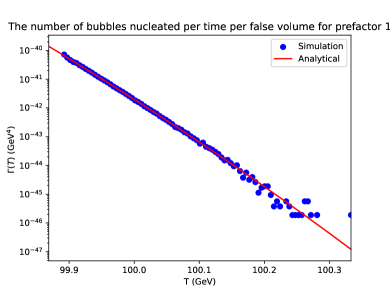
In Fig. 3, we present the average value of $\Gamma_{\rm simulation}$ from 50 repeated simulations and compare it to the value obtained from Eq.(1), using the pre-factor1. Results for the other two pre-factor modes are presented in the Appendix. The comparisons show that Eq.(35) and Eq.(1) generally agree well in most temperature intervals, though deviations are observed at both high and low temperatures. During the early stage of the phase transition, only a few bubbles are randomly generated, which leads to strong statistical fluctuations and in turn results in the deviations at high temperatures. When $T\lesssim 99.88~{}\,\text{GeV}$, the corresponding value of $\Gamma_{\rm simulation}$ diverges and cannot be displayed in the figure. This is because, in the final stage of the phase transition, almost all the region is filled with bubbles. As a result, the theoretical false vacuum fraction approaches zero, but the Monte Carlo simulations give an exact zero, leading to a divergence in Eq.(35). Stacking more simulations can alleviate these statistical effects. However, due to the consumption of computing resources and the fact that $\Gamma_{\rm simulation}$ is in agreement with $\Gamma$ most of the time, it is safe to use above Monte Carlo method to study the statistical measures that characterize bubble kinematics. Thus, except for such special regions, the nucleation rate measured from simulations indeed agree with Eq.(1).

Table 1: Results of the total bubble number from simulation and analytical formula

Total bubble number	Pre-factor 1	Pre-factor 2	Pre-factor 3
Max $N_{\rm tot}^{\rm simulation}$	6373	6091	6972
Min $N_{\rm tot}^{\rm simulation}$	5222	4955	5691
Avg $N_{\rm tot}^{\rm simulation}$	5709	5612	6375
$N_{\rm tot}^{\rm analytic}$	5059	4995	5751
$N_{\rm tot}^{\rm hybrid}$	5722	5624	6388

IV.2 Total Bubble Number

The first statistical measure we study is the total number of bubbles that are generated during the phase transition. Table 1 lists the total number of bubbles for three pre-factor modes obtained from simulation and from the analytical formula. The first three rows show the maximum, minimum, and average numbers of bubbles generated from 50 $\sim$ 60 simulations, respectively. The fourth row shows the results obtained from Eq.(12). The bottom row shows the same results as the fourth row, except that the false vacuum fraction $h$ in Eq.(12) is replaced by $h_{\rm simulation}$ obtained from the simulation (thus denoted as $N_{\rm tot}^{\rm hybrid}$).

It can be seen that the numbers of bubbles generated in pre-factor1 and pre-factor2 are comparable, whereas the number in pre-factor3 is significantly higher than the other two modes, for both the averaged simulation results and theoretical predictions. What is more interesting, however, is the comparison between the simulation result and the theoretical prediction for a fixed pre-factor choice and it is apparent that they do not agree well. The difference is approximately 11.4%, 11.0% and 9.8% for pre-factor1, 2 and 3, respectively.

Figure 4: Comparison between $h$ and $h_{\text{simulation}}$. The red curve, buried under the blue one, is from the analytical formula Eq.(10). The blue curve is obtained by interpolating the stacked simulation data. The intersection point of black dotted line and the red (blue) curve corresponds to the percolation temperature in theory (in simulation). The pink subplot is the zoomed difference between simulation and Eq.(10).

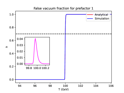
The averaged simulation results $N_{\rm tot}^{\rm simulation}$ are in good agreement with $N_{\rm tot}^{\rm hybrid}$, but differ significantly from $N_{\rm tot}^{\rm analytic}$. The only difference between $N_{\rm tot}^{\rm analytic}$ and $N_{\rm tot}^{\rm hybrid}$ is the false vacuum fraction. Therefore, we present the false vacuum fraction used in analytic and simulation results for pre-factor1 in Fig. 4, denoted by the red and blue curves, respectively.

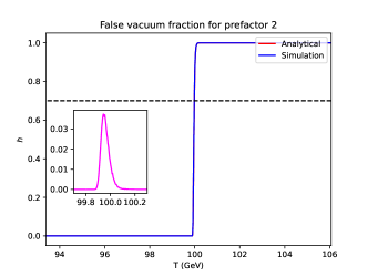
As the false vacuum fraction varies drastically with temperature, it is challenging to clearly distinguish between the red and blue curves in Fig. 4. Thus, we zoom in and show the difference $h_{\rm simulation}-h$. The difference rises to a peak of approximately 0.04 and then decreases to zero. This behavior is crucial for understanding why $N_{\rm tot}^{\rm analytic}$ and $N_{\rm tot}^{\rm hybrid}$ can differ. This confirms that utilizing Eq.(10) will account for the double-counted bubbles and underestimate the false vacuum fraction. For different pre-factor modes, as shown in the Appendix, the results are similar, but the maximum values of $h_{\rm simulation}-h$ are smaller than in pre-factor1.

The black dotted line in Fig. 4 corresponds to a false vacuum fraction of $h=0.7$. The point where this line intersects with the curve corresponds to the percolation temperature, which is typically the temperature at which the phase transition takes place. Due to the sharp decrease in the curves, the simulation-derived percolation temperature (99.986  GeV) is very close to the analytic value (99.989  GeV). This similarity holds true for the other two pre-factor modes (shown in the Appendix), so the difference is not as significant as the difference for the bubble number. The simulation-derived percolation temperatures for pre-factor2 and 3 are respectively 99.980  GeV and 100.105  GeV, and the analytic percolation temperatures are respectively 99.983  GeV and 100.107  GeV.

Figure 5: The distribution of bubble numbers generated in each interval $\left[T_{i},T_{i+1}\right]$ ($T_{i+1}\geq T_{i}$) . The red histogram is from simulations, the blue curve corresponds to the analytical formula $N_{\rm tot}^{\rm analytic}(T_{i})-N_{\rm tot}^{\rm analytic}(T_{i+1})$ and the green one is obtained similarly as the blue one but with the false vacuum fraction replaced by the measured value from simulations $h_{\text{simulation}}$.

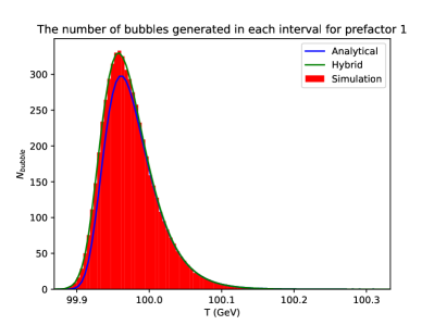
To gain a deeper understanding of the underlying reasons for the variation in the total number of bubbles, we in Fig. 5 illustrate the distribution of the number of bubbles generated within each temperature interval. The red histogram indicates the expected number $N_{\rm tot}^{\rm simulation}(T_{i})-N_{\rm tot}^{\rm simulation}(T_{i+1})$ from simulation, while the blue and green curves are calculated using Eq.(12) in analytical and hybrid approaches, respectively. We can see that the green curve aligns more closely with the simulation results than with the results obtained from the analytical formula. At temperatures above 100 GeV, the simulation results and theoretical predictions exhibit good agreement. However, as the temperature decreases, deviations begin to emerge, reaching a peak at approximately 99.96 GeV. This deviation persists until no bubbles are produced at all.

Hence, the disparity in the total number of bubbles is attributed to the slight variations in $h$ and $\Gamma$, which are magnified by $dt/dT$. As shown in Fig. 4, the discrepancy between $h$ and $h_{\rm simulation}$ becomes apparent as the temperature decreases to 100.2 GeV. However, this deviation is heavily suppressed because of large action, resulting in no disparity in the number of bubbles generated during the initial stage. As the temperature continues to decrease slightly, the action undergoes rapid changes (refer to Fig. 2), so the difference between $h_{\rm simulation}$ and $h$ increases, as well as the number of bubbles generated. The difference between $h$ and $h_{\rm simulation}$ reaches its peak at about 99.96 GeV, resulting in a significant disparity in the number of bubbles. Accordingly, we can also infer that the difference in the total number of bubbles may increase if the phase transition occurs in a temperature region where the action is relatively small and changes gradually.

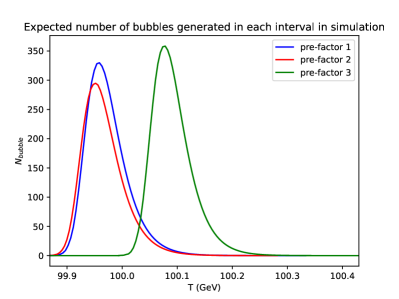
As the green curve agrees with the red histogram very well, we consider the green curve as the simulation results and extract it to assess the impact of different pre-factors in Fig. 6. The blue, red and green curves represent the expected numbers of bubbles generated in each interval for pre-factor1, 2, and 3, respectively. Compared to the pre-factor1 and 2, the phase transition occurred approximately 0.12 GeV earlier for pre-factor3. The maximum value of bubble number for pre-factor3 is approximately 60 larger than pre-factor2, and about 20 larger than pre-factor1.

Figure 6: Comparison between the expected numbers of bubbles generated in each interval in simulation for three pre-factors. The blue, red and green curves are for pre-factor1, 2 and 3, respectively.

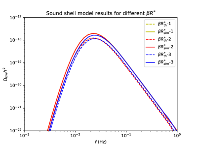
As the small difference of false vacuum fraction will result in a non-negligible difference in the total number of bubbles and consequently affect the bubble mean separation $R^{*}$, we expect it could accordingly change the gravitational wave spectra. The calculations of the gravitational wave spectra are done in the sound shell model, and the results are presented in Fig. 7. There the dashed curves denote the spectra obtained with $\beta R^{*}=(8\pi)^{1/3}v_{\rm w}$ while the solid curves with $\beta R^{*}_{\text{simulation}}$. It is observed that there is an enhancement in gravitational wave spectra. Compared to the usually adopted value, the peak value of gravitational wave spectra for three pre-factors have an increase by a factor of 1.60, 1.58, and 1.41, respectively. This primarily arises from the term in Eq.(20), from the combined effect of the denominator and the integrand.

Figure 7: Gravitational wave spectra for different $\beta R^{*}$. The dashed curves are the results of the original sound shell model and the solid curves are the results with improved $\beta R^{*}$. The results for pre-factor1 are covered by those for pre-factor2.

IV.3 Bubble Lifetime Distribution

The gravitational wave spectra can also be modified by the change in the bubble lifetime distribution, which can be measured directly from simulations and compared with the corresponding analytical formula. To measure it from simulations, we compute the destruction temperature $T_{\rm death}$ for each bubble, and define the lifetime for a bubble as

$$\bar{t}=\hat{t}(T_{\rm death})-\hat{t}(T_{\rm birth}),$$ (36)

where $\hat{t}$ represents the solution of the differential equation described in Eq.(33). By dividing the interval $\left[\min(\beta\bar{t}),\max(\beta\bar{t})\right]$ into many small intervals $\left[\beta\bar{t}_{i},\beta\bar{t}_{i}+\beta\Delta\bar{t}\right]$, where

$$\beta=\left.-\frac{d}{dt}\ln\Gamma\right|_{t=\hat{t}(T_{f})},$$ (37)

we can count the number of bubbles $N_{i}$ in each interval. Thus the probability density for a bubble having the lifetime $\bar{t}_{i}$ is

$$\nu_{i}=N_{i}/(N_{\rm tot}\beta\Delta\bar{t}).$$ (38)

Figure 8: The distribution of bubble lifetime. The red line is the analytical formula Eq.(18) and the blue histogram is the simulation result. The $\beta\bar{t}$ for each rectangle is the center value of the interval.

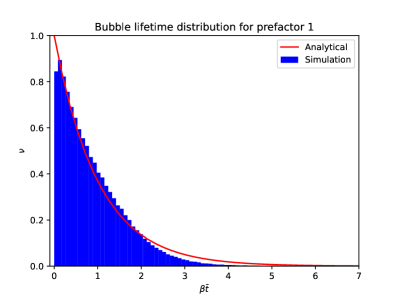
Fig. 8 shows the bubble lifetime distribution for pre-factor1 and the results for other two modes are presented in the Appendix. The red curve represents Eq.(18), while the blue histogram represents the simulation result. We see that that the two results do not exhibit good agreement. Eq.(18) tends to underestimate the distribution of bubble lifetimes when $0.14\leq\beta\bar{t}\leq 2$, while overestimating the distribution in other regions. This suggests that the bubble lifetime distribution is not an ideal exponential distribution as described by Eq.(18). This deviation could be explained by noting that, in the derivation of $\nu_{\rm th}$, a constant distance $L$ is utilized. However, it is actually possible for a bubble to spontaneously appear between the phase boundary and the bubble we are studying, leading to a sudden decrease in $L$ and resulting in a shorter lifetime. As a result, the number of long-lived bubbles is suppressed, and their corresponding count is transferred to the range of shorter-lived bubbles ($0.14\leq\beta\bar{t}\leq 2$). Furthermore, due to the normalization of $\nu$, the area below $\nu$ equals to 1. Thus, this transferred counting will result in a decrease in the areas of the near zero interval. Similar findings are also reported in Ref.Hijazi (2022), where the definition of bubble lifetime slightly differs. To make sure this is not due to a numerical artifact, we examined the bubble birth time within near zero interval and observed that it is not concentrated within a particular range.

Given the distinctive behavior of the bubble lifetime distribution, we anticipate that it will result in a modification of gravitational wave spectra. By inserting our simulation results $R^{*}_{\rm simulatiom}$ and $\nu_{\rm simulation}$, we get the final gravitational wave spectra and compare it with the original spectra in Fig. 9. The dashed curves in this figure are obtained with the original set of analytical inputs while the solid curves are obtained with inputs from numerical simulations where the bubble lifetime distribution is replaced by $\nu_{\rm simulation}$.

Figure 9: The gravitational wave spectra calculated by combining our simulation results and sound shell model. The dashed curves are the results of the original spectra and the solid curves are obtained with simulation results. The results for pre-factor1 are covered by those for pre-factor2. Here we set the alpha factor in front of the bubble wall $\alpha_{+}$ as 0.0046 Hindmarsh and Hijazi (2019).

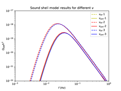
From Fig. 9 we find that: (1) the gravitational wave spectra are almost the same for three different pre-factors; (2) the peak of the spectra shifts to a higher frequency compared with the original spectra and the original one overestimates the gravitational wave in the whole range of $f$. This suppression effect could be explained by noting that $\nu$ and $|A|^{2}$ are all rapidly decreasing to a small number when the independent variable deviated from the origin Guo et al. (2021) and so the main contribution to $\mathcal{P}_{v}$ comes from a small $f$ (which is equivalent to the $qR^{*}$) and small $\beta\bar{t}$, which exactly corresponds to one of the suppression interval in Fig. 8.

Table 2: Deviation of characteristic physical quantities

Uncertainty	pre-factor1	pre-factor2	pre-factor3
$T_{\rm p}$	0.003%	0.003%	0.002%
$\beta R^{*}$	8.1%	7.9%	5.9%
$N_{\rm tot}$	11.4%	11.0%	9.8%
$f^{\rm peak}_{\beta R^{*}}$	11.8%	12.0%	14.1%
$\Omega_{\rm GW}h^{2}_{\beta R^{*}}$	37.6%	36.5%	28.9%
$f^{\rm peak}_{\rm sim}$	36.4%	36.4%	35.1%
$\Omega_{\rm GW}h^{2}_{\rm sim}$	334.0%	330.8%	336.7%

Finally, we list all the deviations of characteristic physical quantities $|(C_{\rm th}-C_{\rm sim})|/C_{\rm sim}$ in Table II, where the row $f^{\rm peak}_{\beta R^{*}}$ shows the uncertainty of the peak frequency of the sound shell model results with different $\beta R^{*}$ and $\Omega_{\rm GW}h^{2}_{\beta R^{*}}$ shows the corresponding uncertainty of the gravitational wave spectra peak values. The rows $f^{\rm peak}_{\rm sim}$ and $\Omega_{\rm GW}h^{2}_{\rm sim}$ are similar with the above two.

V Conclusion

In this work we conducted simulations of bubble nucleation and compare the results with the usually adopted analytical formula. Our major findings are the following:

1. The false vacuum fraction has a tiny difference between the simulation results and analytical formula.

2. The analytical formula can not describe the total number of bubbles well, causing an error of about 10%. This deviation will lead to an enhancement of the gravitational wave spectra.

3. The difference for the total number of bubbles is the combined effect of the Euclidean action and the false vacuum fraction and is magnified by $dt/dT$, which implies the importance of the description of the false vacuum fraction.

4. Three different pre-factors do not lead to significantly different bubble lifetime distributions and the real bubble lifetime distribution is not an exponential distribution, which will cause a suppression effect for the gravitational wave spectra in the whole range in the sound shell model.

So our current theoretical framework falls short in fully describing bubble kinematics, as evidenced by our results. This leads to a theoretical uncertainty in the prediction of gravitational waves. To address this, in our future work we will improve the existing theoretical model, especially the part related to the lifetime distribution. It is crucial to dedicate more attention to refining the existing theoretical framework, in order to calculate gravitational waves with high precision.

Appendix

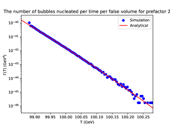
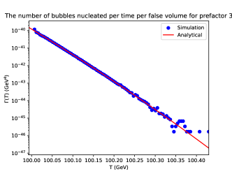
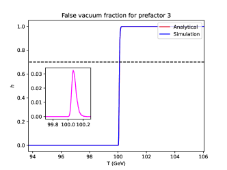
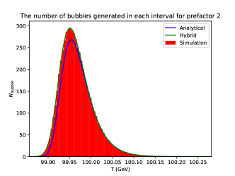
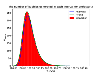
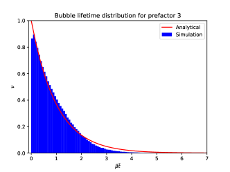
In Figs. 10-13 we compare the simulated results with the theoretical values on the bubble nucleation rate, the false vacuum fraction, the bubble number generated in small intervals and the bubble lifetime distribution for pre-factor 2 and 3.

Figure 10: Same as Fig. 3, but for pre-factor2 and pre-factor3.

Figure 11: Same as Fig. 4, but for pre-factor2 and pre-factor3.

Figure 12: Same as Fig. 5, but for pre-factor2 and pre-factor3.

Figure 13: Same as Fig. 8, but for pre-factor2 and pre-factor3.

References

- Abbott et al. (2016) B. P. Abbott, R. Abbott, T. Abbott, M. Abernathy, F. Acernese, K. Ackley, C. Adams, T. Adams, P. Addesso, R. Adhikari, et al., Physical review letters 116, 061102 (2016).
- Weir (2018) D. J. Weir, Philosophical Transactions of the Royal Society A: Mathematical, Physical and Engineering Sciences 376, 20170126 (2018).
- Mazumdar and White (2018) A. Mazumdar and G. White, arXiv preprint arXiv:1811.01948 (2018).
- Bertone et al. (2020) G. Bertone, D. Croon, M. Amin, K. K. Boddy, B. Kavanagh, K. J. Mack, P. Natarajan, T. Opferkuch, K. Schutz, V. Takhistov, et al., SciPost Physics Core 3, 007 (2020).
- Abbott et al. (2017) B. P. Abbott, R. Abbott, T. D. Abbott, M. Abernathy, F. Acernese, K. Ackley, C. Adams, T. Adams, P. Addesso, R. Adhikari, et al., Physical review letters 118, 121101 (2017).
- Scientific et al. (2019) L. Scientific, B. Abbott, R. Abbott, T. Abbott, S. Abraham, F. Acernese, K. Ackley, C. Adams, V. Adya, C. Affeldt, et al., Physical Review D 100, 061101 (2019).
- Amaro-Seoane et al. (2017) P. Amaro-Seoane, H. Audley, S. Babak, J. Baker, E. Barausse, P. Bender, E. Berti, P. Binetruy, M. Born, D. Bortoluzzi, et al., arXiv preprint arXiv:1702.00786 (2017).
- Gong et al. (2015) X. Gong, Y.-K. Lau, S. Xu, P. Amaro-Seoane, S. Bai, X. Bian, Z. Cao, G. Chen, X. Chen, Y. Ding, et al., in Journal of Physics: Conference Series (IOP Publishing, 2015), vol. 610, p. 012011.
- Luo et al. (2016) J. Luo, L.-S. Chen, H.-Z. Duan, Y.-G. Gong, S. Hu, J. Ji, Q. Liu, J. Mei, V. Milyukov, M. Sazhin, et al., Classical and Quantum Gravity 33, 035010 (2016).
- Athron et al. (2023a) P. Athron, C. Balázs, A. Fowlie, L. Morris, and L. Wu (2023a), eprint 2305.02357.
- Han et al. (2021) X.-F. Han, L. Wang, and Y. Zhang, Physical Review D 103, 035012 (2021).
- Guo et al. (2021) H.-K. Guo, K. Sinha, D. Vagie, and G. White, Journal of Cosmology and Astroparticle Physics 2021, 001 (2021).
- Yang et al. (2023) J. Yang, R. Zhou, and L. Bian, Physics Letters B 839, 137822 (2023).
- Xiao et al. (2023) Y. Xiao, J. M. Yang, and Y. Zhang (2023), eprint 2307.01072.
- Balázs et al. (2023) C. Balázs, Y. Xiao, J. M. Yang, and Y. Zhang (2023), eprint 2301.09283.
- Vaskonen (2017) V. Vaskonen, Physical Review D 95, 123515 (2017).
- Beniwal et al. (2019) A. Beniwal, M. Lewicki, M. White, and A. G. Williams, Journal of High Energy Physics 2019, 1 (2019).
- Kang et al. (2018) Z. Kang, P. Ko, and T. Matsui, Journal of High Energy Physics 2018, 1 (2018).
- Chala et al. (2018) M. Chala, C. Krause, and G. Nardini, Journal of High Energy Physics 2018, 1 (2018).
- Alves et al. (2020) A. Alves, D. Gonçalves, T. Ghosh, H.-K. Guo, and K. Sinha, Journal of High Energy Physics 2020, 1 (2020).
- Alves et al. (2019) A. Alves, T. Ghosh, H.-K. Guo, K. Sinha, and D. Vagie, Journal of High Energy Physics 2019, 1 (2019).
- Chao et al. (2017) W. Chao, H.-K. Guo, and J. Shu, Journal of Cosmology and Astroparticle Physics 2017, 009 (2017).
- Kosowsky et al. (1992) A. Kosowsky, M. S. Turner, and R. Watkins, Physical Review D 45, 4514 (1992).
- Kosowsky and Turner (1993) A. Kosowsky and M. S. Turner, Physical Review D 47, 4372 (1993).
- Jinno and Takimoto (2017) R. Jinno and M. Takimoto, Physical Review D 95, 024009 (2017).
- Hindmarsh et al. (2015) M. Hindmarsh, S. J. Huber, K. Rummukainen, and D. J. Weir, Physical Review D 92, 123009 (2015).
- Hindmarsh et al. (2017) M. Hindmarsh, S. J. Huber, K. Rummukainen, and D. J. Weir, Physical Review D 96, 103520 (2017).
- Hindmarsh et al. (2014) M. Hindmarsh, S. J. Huber, K. Rummukainen, and D. J. Weir, Physical Review Letters 112, 041301 (2014).
- Hindmarsh (2018) M. Hindmarsh, Physical Review Letters 120, 071301 (2018).
- Hindmarsh and Hijazi (2019) M. Hindmarsh and M. Hijazi, Journal of Cosmology and Astroparticle Physics 2019, 062 (2019).
- Jinno and Takimoto (2019) R. Jinno and M. Takimoto, Journal of Cosmology and Astroparticle Physics 2019, 060 (2019).
- Konstandin (2018) T. Konstandin, Journal of Cosmology and Astroparticle Physics 2018, 047 (2018).
- Cai et al. (2023a) R.-G. Cai, S.-J. Wang, and Z.-Y. Yuwen, arXiv preprint arXiv:2305.00074 (2023a).
- Kosowsky et al. (2002) A. Kosowsky, A. Mack, and T. Kahniashvili, Physical Review D 66, 024030 (2002).
- Dolgov et al. (2002) A. D. Dolgov, D. Grasso, and A. Nicolis, Physical Review D 66, 103505 (2002).
- Caprini et al. (2009) C. Caprini, R. Durrer, and G. Servant, Journal of Cosmology and Astroparticle Physics 2009, 024 (2009).
- Yang and Bian (2022) J. Yang and L. Bian, Phys. Rev. D 106, 023510 (2022), eprint 2102.01398.
- Di et al. (2021) Y. Di, J. Wang, R. Zhou, L. Bian, R.-G. Cai, and J. Liu, Phys. Rev. Lett. 126, 251102 (2021), eprint 2012.15625.
- Croon et al. (2021) D. Croon, O. Gould, P. Schicho, T. V. Tenkanen, and G. White, Journal of High Energy Physics 2021, 1 (2021).
- Athron et al. (2023b) P. Athron, C. Balazs, A. Fowlie, L. Morris, G. White, and Y. Zhang, JHEP 01, 050 (2023b), eprint 2208.01319.
- Andreassen et al. (2017) A. Andreassen, D. Farhi, W. Frost, and M. D. Schwartz, Physical Review D 95, 085011 (2017).
- Dunne and Min (2005) G. V. Dunne and H. Min, Physical Review D 72, 125004 (2005).
- Ekstedt (2022) A. Ekstedt, The European Physical Journal C 82, 173 (2022).
- Guth and Weinberg (1981) A. H. Guth and E. J. Weinberg, Physical Review D 23, 876 (1981).
- Enqvist et al. (1992) K. Enqvist, J. Ignatius, K. Kajantie, and K. Rummukainen, Physical Review D 45, 3415 (1992).
- Athron et al. (2023c) P. Athron, C. Balázs, and L. Morris, Journal of Cosmology and Astroparticle Physics 2023, 006 (2023c).
- Cai et al. (2017) R.-G. Cai, M. Sasaki, and S.-J. Wang, Journal of Cosmology and Astroparticle Physics 2017, 004 (2017).
- Linde (1983) A. D. Linde, Nuclear Physics B 216, 421 (1983).
- Rubakov (2009) V. Rubakov, in Classical Theory of Gauge Fields (Princeton University Press, 2009).
- Imai et al. (1985) H. Imai, M. Iri, and K. Murota, SIAM Journal on Computing 14, 93 (1985).
- Hijazi (2022) M. Hijazi, arXiv preprint arXiv:2208.10636 (2022).
- Espinosa et al. (2010) J. R. Espinosa, T. Konstandin, J. M. No, and G. Servant, Journal of Cosmology and Astroparticle Physics 2010, 028 (2010).
- Cai et al. (2023b) R.-G. Cai, S.-J. Wang, and Z.-Y. Yuwen, Phys. Rev. D 108, L021502 (2023b), eprint 2305.00074.
- Gowling and Hindmarsh (2021) C. Gowling and M. Hindmarsh, Journal of Cosmology and Astroparticle Physics 2021, 039 (2021).
- Cutting et al. (2020) D. Cutting, M. Hindmarsh, and D. J. Weir, Phys. Rev. Lett. 125, 021302 (2020), eprint 1906.00480.
- Adams (1993) F. C. Adams, Physical Review D 48, 2800 (1993).
- Dine et al. (1992) M. Dine, R. G. Leigh, P. Y. Huet, A. D. Linde, and D. A. Linde, Phys. Rev. D 46, 550 (1992), eprint hep-ph/9203203.
- Lewicki et al. (2022) M. Lewicki, M. Merchand, and M. Zych, Journal of High Energy Physics 2022, 1 (2022).
- Konstandin et al. (2014) T. Konstandin, G. Nardini, and I. Rues, Journal of Cosmology and Astroparticle Physics 2014, 028 (2014).
- Wang et al. (2020) X. Wang, F. P. Huang, and X. Zhang, arXiv preprint arXiv:2011.12903 (2020).
- Mégevand and Sánchez (2010) A. Mégevand and A. D. Sánchez, Nuclear physics B 825, 151 (2010).
- Jinno et al. (2019) R. Jinno, T. Konstandin, and M. Takimoto, Journal of Cosmology and Astroparticle Physics 2019, 035 (2019).
- Gould et al. (2021) O. Gould, S. Sukuvaara, and D. Weir, Physical Review D 104, 075039 (2021).