Stability Analysis of Non-Linear Classifiers using Gene Regulatory Neural Network for Biological AI

Abstract

The Gene Regulatory Network (GRN) of biological cells governs a number of key functionalities that enables them to adapt and survive through different environmental conditions. Close observation of the GRN shows that the structure and operational principles resembles an Artificial Neural Network (ANN), which can pave the way for the development of Biological Artificial Intelligence. In particular, a gene’s transcription and translation process resembles a sigmoidal-like property based on transcription factor inputs. In this paper, we develop a mathematical model of gene-perceptron using a dual-layered transcription-translation chemical reaction model, enabling us to transform a GRN into a Gene Regulatory Neural Network (GRNN). We perform stability analysis for each gene-perceptron within the fully-connected GRNN sub-network to determine temporal as well as stable concentration outputs that will result in reliable computing performance. We focus on a non-linear classifier application for the GRNN, where we analyzed generic multi-layer GRNNs as well as E.Coli GRNN that is derived from trans-omic experimental data. Our analysis found that varying the parameters of the chemical reactions can allow us shift the boundaries of the classification region, laying the platform for programmable GRNNs that suit diverse application requirements.

[*]aratwatte2@huskers.unl.edu Article

In recent years the significance of artificial intelligence has been steadily rising, driven by the development of numerous algorithms that are applicable across various domains. As we envision a future of "AI everywhere", we are faced with the prospects of applying AI into media that is beyond silicon technology, such as wet biological environments. In this study our objective is to propose a paradigm of Biological AI that is built from the gene regulatory process. Realizing a vision of Biological machine AI, can result in novel theranostic applications for disease detection and treatment as well as new bio-hybrid computing systems that integrates biological cells with silicon technology.

Introduction

In recent years, the field of Artificial intelligence (AI) has developed rapidly resulting in sophisticated learning algorithms that have benefited a plethora of applications (e.g., manufacturing, economics, computer vision, robotics, etc.) (chowdhury2012advantages). Inspired by the functions of neurons, the ultimate vision of AI is to create human-like intelligence that one day will have a working capacity close to the brain. Based on the system applications, AI can be categorized into software or hardware-based. Software-based AI includes various forms of algorithms that depends on their structure as well as training process (e.g., convolutional neural networks (li2021survey), recurrent neural networks (medsker2001recurrent), where a novel applications is large language models such as Generative Pre-trained Transformer (GPT) (kasneci2023chatgpt).

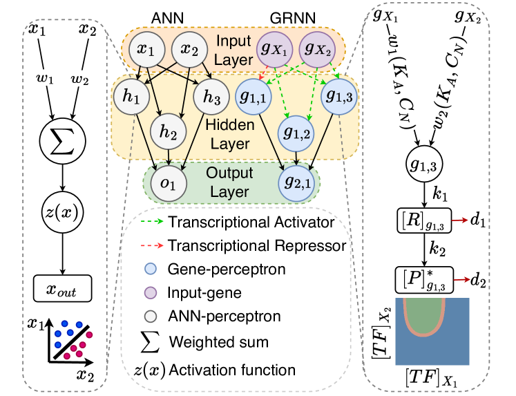
Figure 1: Illustration of mapping between components of ANN to GRNN. In this depiction, $w_{i}$ and $w_{i}(K_{A},C_{N})$ represent the weights of a perceptron in ANN and GRNN, respectively, while activation function $z(x)$ is equivalent to a combination of the transcription process of RNA concentration $[R]_{i}$ as well as translation of maximum-stable protein concentration $[P]_{i}^{*}$. The chemical reactions are governed by the transcriptions rate $k_{1}$, translation rate $k_{2}$, degradation rate of RNA $d_{1}$ and degradation rate of protein $d_{2}$.

Neuromorphic processors is a hardware-based AI platform that architecturally consists of neurons and synapses constructed from memristor devices that communicate based on encoded neural spikes. (schuman2022opportunities). Presently, the vast majority of AI machines are constructed using instruction-encoded circuits and silicon-based semiconductors and nanotechnology (nesbeth2016synthetic), (akan2016fundamentals), (akan2023internet). While this enables more efficient computer systems that have capabilities of learning and computing, it also results in significant challenges such as deployments in wet non-silicon mediums (e.g., biological mediums), as well as utilizing large amounts of energy. (schwenk2005training).

Current research has aimed to address these challenges and one direction taken is through Biological AI, where computing are performed through living biological cells (balasubramaniam2023realizing), (bi2021survey). A recent examples is the DishBrain, where the system is composed of living neurons that can be trained to play the game of "Pong" on a computer (kagan2022vitro). In other works, ANNs have been programmed into bacterial cells (becerra2022computing), (li2021synthetic). Similarly, molecular circuits programmed to behave like ANN have also been proposed, and one example is the Bio-molecular Neural Network (BNN) (samaniego2021signaling). The underlying basis for all these approaches, is the communication of molecules (soldner2020survey) that operates as part of the chemical reactions to enable computing operations.

From the perspective of Gene Regulatory Networks (GRN), there has been a connection between its structure and the operation of a ANN. In our recent work (somathilaka2023revealing), we developed a model that transforms the gene-gene interaction within the GRN using weights, forming a GRNN while also exploring the impact of structural changes on the computing capacity. In this study, we investigate the behaviour of a fully-connected GRNN derived from a GRN, focusing on the stability analysis of the gene translation and transcription process during its computing operation. The stability analysis focuses on each perceptron of the GRNN, which we term as gene-perceptron. Figure 1 illustrates the mapping from ANN to GRNN. In a conventional ANN, a perceptron takes multiple inputs ($x_{1}$ and $x_{2}$) and computes their weighted summation ($\sum$) that goes through an activation function ($z(x)$). In the context of the GRNN, the weights are represented as Transcription Factors (TF) concentration corresponding to half-maximal RNA concentration ($K_{A}$) and gene-product copy number ($C_{N}$), which individually impact RNA and protein concentrations. Input-genes ($g_{X_{1}}$ and $g_{X_{2}}$) have TFs that binds to the promoter region of the gene-perceptron $g_{1,i}$, which transcribes to RNA ($R_{i}$) and then translate to protein ($P_{i}$). This can be considered as a weighted summation, which results in regulatory effects on gene expression within the gene-perceptron. Based on the stability of each gene-perceptron at the steady state, the maximum-stable protein concentration ($[P]^{*}$), represents the output.

We mathematically model chemical reactions of the transcription and translation process of a gene-perceptron, which we term as the dual-layered transcription-translation reaction model (from here on we simply term this as dual-layered chemical reaction model). The dual-layered chemical reaction model can be integrated with trans-omic data model (transcriptome and proteome) and the cellular GRN in order for us to identify active genes for the specific environments, which will be the basis for us to create the GRNN.

Based on this platform, we will perform stability analysis at the steady-state of molecular production (RNA and protein) for the gene-perceptron. Once we prove the stability of the gene-perceptron, as an application we focus on a non-linear classifier relying on the maximum-stable protein concentration for different concentrations of TFs that acts as inputs. To evaluate the model’s performance, we analyze two generic multi-layer GRNN networks and an E.Coli GRNN. We also show that we can manipulate and shift the classification areas based on different parameter configurations.

The contributions of this study can be outlined as follows:

• Developing GRNN inspired from ANN structures using dual-layer chemical reaction models: Using the dual-layered chemical reaction model, we show that gene transcription and RNA translation process exhibit a sigmoidal-like molecular concentration dynamics at their stable points. This behavior is governed by the weights, which is a function of gene product copy number and transcription factors TFs concentration corresponding to the half-maximal RNA concentration.

• Stability analysis of GRNN: We developed full mathematical models derived from the chemical reactions and apply Lyapunov’s stability analysis for the gene-perceptron to determine stable protein concentration as well as temporal production that will facilitate reliable GRNN computing.

• GRNN application for non-linear classifiers: Using the stability analysis, we are able to determine the decision boundaries of the derived GRNNs to classify data within regions of protein concentration output. By varying parameters of the chemical reactions, we demonstrate how the classification area can be shifted, which can serve as a tool for engineering the GRN for several non-linear classifiers based on the application’s requirements.

System Modeling

Figure 2: Illustration of dual-layered transcription-translation chemical reaction model of the gene-perceptron. Each components corresponds to the synthesis and degradation of RNA and protein for the $j^{\text{th}}$ gene-perceptron in the $i^{\text{th}}$ layer ($g_{i,j}$) of the GRNN. Here, RnpB, SsrA and SsrS are examples for non-coding RNA (ncRNA). Examples of energy-dependent proteases include Lon, HflB, ClpXP and HslUV. Active TF, RNAP, PNPase, RNase E and tRNA corresponds to active TFs, RNA polymerase, Polyribonucleotide phosphorylase, Ribonuclease E and transfer RNA, respectively.

This section describes the mathematical models for the gene transcription and translation within gene-perceptrons, employing a dual-layered chemical reaction model (Figure 2) that breaks down the steps of the translation and transcription process. The production of RNAs depends on RNA polymerase, TFs and $\sigma$ factors that binds to the promoter ($Prom$) (wang2021direct), as well as the dissociation constant ($k_{d}$). Once the TF binds to the promoters $Prom$, the transcription begins at the rate of $k_{1}$. This is followed by the RNA degradation at the rate of $d_{1}$ based on their half-life value (bernstein2002global), RNA binding proteins (holmqvist2018rna) as well as the degradosome components that includes RNase E, RNA helicase, as well as PNPase (tejada2020bacterial). Following the transcription of the RNAs is the translation into protein, which occurs at the rate of $k_{2}$ facilitated by Ribosome and Transfer RNA (tRNA). Once the RNA is translated, the protein molecules start to degrade gradually at the rate of $d_{2}$. Significant factors that affect the degradation of protein are non-coding RNA, as well as energy-dependent and energy-independent Proteases. Overall, to maintain the concentration stability in the cell, RNAs and protein production are balanced by the degradation process.

By taking the dual-layered chemical reactions model into account, we model the concentration changes at the transcriptome and proteome using mathematical models. These models, enable us to assess the stability of the gene-perceptron expression through the eigenvalue method and determine the stabilization time using the Lyapunov stability theorem. After determining if a particular gene-percepton expression is stable, we determine the stability of the entire GRNN. Then, based on the application study, the classification ranges for each gene-perceptron in a network is determined at the equilibrium maximum-stable protein concentration state. Based on the sigmoidal input-output behavior and adjustable threshold, we deduce that gene-perceptrons in the GRNN consist of conventional NN properties. For the overview of the algorithm mentioned above, please refer to Figure 3.

Figure 3: Flow chart for the calculation of classification areas as well as stability based on the dual-layred transcription-translation chemical reaction model of each gene-perceptron.

Modelling Transcription of a Gene

In this section, we discuss transcription and the corresponding RNA concentration model. During the transcription process, the RNA polymerase and TFs bind to the promoter region and then the $\sigma$ factor attaches to the promoter region and unwinds the DNA (cao2020stochastic). This is followed by the $\sigma$ factor release from the polymerase, allowing for the elongation of the RNA chain. Based on (santillan2008use), the concentration change over time $t$ of RNA for a particular gene-perceptron $i$ can be expressed as follows (chemical species are represented using uppercase letters (e.g., $X$), and their corresponding concentration is enclosed within brackets (e.g., $[X]$))

$$\dfrac{d[R]_{i}}{dt}=k_{1_{i}}C_{N_{i}}\dfrac{[TF]^{n}}{K_{A_{i}}^{n}+[TF]^{n}}-d_{1_{i}}[R]_{i}.$$ (1)

The gene-perceptron is activated by the TF, where $[R]_{i},$ $k_{1_{i}}$, $[TF]$, $d_{1_{i}}$, $n$, $C_{N_{i}}$ and $K_{A_{i}}$ are the RNA concentration, transcription rate, concentration of TFs, degradation rate of RNA, Hill coefficient, gene product copy number and TF concentration when the production of RNA is at the half maximal point for gene-perceptron $i$, respectively.

Given the initial RNA concentration transcribed by a gene-perceptron is $[R]_{i}(0)$ (i.e., $[R]_{i}(t=0)=[R]_{i}(0)$), the solution of Eq. 1 is derived as follows

$$[R]_{i}=\dfrac{k_{1_{i}}C_{N_{i}}}{d_{1_{i}}}\left(\dfrac{[TF]^{n}}{[TF]^{n}+K_{A_{i}}^{n}}\right)(1-e^{d_{1_{i}}t})+[R]_{i}(0)e^{d_{1_{i}}t}.$$ (2)

In contrast, in the event that the gene-perceptron is repressed by the TF, the RNA concentration changes over time $t$ is represented as follows,

$$\dfrac{d[R]_{i}}{dt}=k_{1_{i}}C_{N_{i}}\dfrac{K_{A_{i}}^{n}}{K_{A_{i}}^{n}+[TF]^{n}}-d_{1_{i}}[R]_{i}.$$ (3)

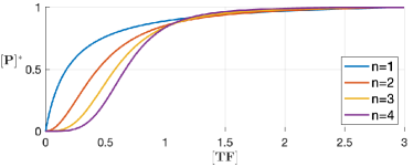
Eq. 1 and 3 is expressed as a mass balance differential equation with the difference between the RNA synthesis, which is modelled using the Hill function integrated with the degradation process of the RNA (yugi2019rate), (alon2019introduction), (thompson2020multiple). The Hill coefficient $n$ represents the number of TF molecules that bind simultaneously to the promoter $Prom$ with $K_{d}$ reaction dissociation constant when the gene-perceptron is transcribing RNA (santillan2008use) and is represented as $Prom+n\,\,TF\stackrel{{\scriptstyle K_{d}}}{{\rightleftharpoons}}Prom_{n.TF}$. The Hill coefficient is critical for the sigmoidal input-output characteristics of the gene-perceptron, as depicted in Figure 4. According to the plot, we can see that when we increase the hill coefficient, the sigmoidicity increase for the maximum-stable protein concentration ($[P]^{*}$) over the input-gene concentration ($[TF]$). Thus, when a gene-perceptron possesses a higher hill coefficient, it exhibits more sigmoidal-like behavior. (for our analytical model we consider $n=1$).

Figure 4: Sigmoidicity fluctuations for different Hill coefficients.

Modelling Translation of a RNA

In this section, we describe RNA-to-protein translation and associated models. Initially, the ribosome and tRNAs form a complex that draws the amino acids in the polypeptide chain to attach to the first codon position of the RNA (saito2020translational). This is followed by the tRNAs adding amino acids one by one to form a polypeptide chain while moving along the RNA (xu2022functions). Once the stop codon is detected, the polypeptide chain is released, dissociating the ribosome complex from the RNA and forming the protein (marintchev2012fidelity). This process can be summarized through the protein concentration change over time, and is modelled as follows for a particular gene-perceptron $i$:

$$\dfrac{d[P]_{i}}{dt}=k_{2_{i}}[R]_{i}-d_{2_{i}}[P]_{i},$$ (4)

where $[P]_{i},k_{2_{i}}$ and $d_{2_{i}}$ are the protein concentration, translation rate and degradation rate of protein for gene-perceptron $i$. Moreover, $[R]_{i}$ is the concentration of RNA from Eq. 1, and the TF activates the gene-perceptron $i$ based on Eq. 3 if the TF represses the gene-perceptron. Similar to Eq. 1 and 3, Eq. 4 is modelled based on mass-balance differential equation taking the difference between the RNA produced at the transcriptome level which is translated into protein at the rate of $k_{2_{i}}$ and the amount of protein that is degraded at the rate of $d_{2_{i}}$ due to the factors presented in Figure 2. Provided that the initial protein concentration translated by a RNA for gene-perceptron $i$ is $[P]_{i}(0)$ (i.e., $[P]_{i}(t=0)=[P]_{i}(0)$), the solution of Eq. 4 is given by

$$[P]_{i}=\dfrac{k_{1_{i}}k_{2_{i}}C_{N_{i}}}{d_{1_{i}}}\left(\dfrac{[TF]^{n}}{[TF]^{n}+K_{A_{i}}^{n}}\right)\left(\dfrac{1}{d_{2_{i}}}-\dfrac{e^{d_{1_{i}}t}}{d_{1_{i}}+d_{2_{i}}}\right)\\ +[R]_{i}(0)k_{2_{i}}\left(\dfrac{e^{d_{1_{i}}t}}{d_{1_{i}}+d_{2_{i}}}\right)+e^{-d_{2_{i}}t}[P]_{i}(0)-e^{-d_{2_{i}}t}\\ \times[R]_{i}(0)k_{2_{i}}\dfrac{1}{(d_{1_{i}}+d_{2_{i}})}-e^{-d_{2_{i}}t}\dfrac{k_{1_{i}}k_{2_{i}}C_{N_{i}}}{d_{1_{i}}}\\ \left(\dfrac{[TF]^{n}}{[TF]^{n}+K_{A_{i}}^{n}}\right)\times\left(\dfrac{1}{d_{2_{i}}}-\dfrac{1}{(d_{1_{i}}+d_{2_{i}})}\right).$$ (5)

Methods

This section introduces the mathematical models for the stability analysis and RNA/Protein concentration changes over time, and subsequently demonstrates how to apply these mathematical models in the GRNNs.

Gene Expression Stability Analysis

In this section, we discuss the approach towards analyzing the stability of the gene-perceptron expression. Our view of the stability of the gene-perceptron is when the RNA transcription as well as the protein translation concentrations reach maximum over time and remain stable at that level exhibiting a sigmoidal behavior. To confirm the existence of transcription and translation upper bounds, we use eigenvalue-based stability analysis. This, in turn, ensures a stable classification region of the GRNN due to a protein concentration with minimum fluctuations that can result in minimized computing errors. Moreover, another crucial property that should be considered in GRNN computing is the time it takes the GRNN to reach stability, which is investigated using the Lyapunov function in the following sections.

Stability of Gene-Perceptron based on Eigenvalues

The stability of the gene-perceptron is governed by the concentration changes of the gene expression as well as protein translation using the Jacobian matrix of Eq. 1 and 4, which enables us to define the equilibrium point based on the eigenvalues. While we have only considered the case of gene transcription in Eq. 1, our approach is also applicable for repression process defined in Eq. 3. Since we are analysing the stability of the gene-perceptron at the equilibrium point, we can represent the maximum-stable RNA $[R]_{i}^{*}$ and protein $[P]_{i}^{*}$ concentration as follows:

$$[R]_{i}^{*} =\dfrac{k_{1_{i}}C_{N_{i}}}{d_{1_{i}}}\left(\dfrac{[TF]^{n}}{[TF]^{n}+K_{A_{i}}^{n}}\right),$$ (6)

$$[P]_{i}^{*} =\dfrac{k_{1_{i}}k_{2_{i}}C_{N_{i}}}{d_{1_{i}}d_{2_{i}}}\left(\dfrac{[TF]^{n}}{[TF]^{n}+K_{A_{i}}^{n}}\right).$$ (7)

The maximum-stable RNA and protein concentrations are determined for different TF concentrations. Additionally, we can vary gene-specific parameters such as $C_{N_{i}}$ to achieve different non-linear classification ranges (kim2011measuring), implying that by engineering the cell, we can change its decision-making process.

To determine the eigenvalues of Eq. 1 and 4 at the equilibrium points of Eq. 6 and 7, we use the Jacobian matrix given in Eq. 24 (please see Appendix). Hence, the eigenvalues are $\lambda_{1}=-d_{1_{i}}$ and $\lambda_{2}=-d_{2_{i}}$. Since all the eigenvalues ($\lambda_{1}$ and $\lambda_{2}$) are negative, we can conclude that the gene-perceptron reaches maximum-stable concentration level.

Stability of a Gene-Perceptron using Lyapunov function

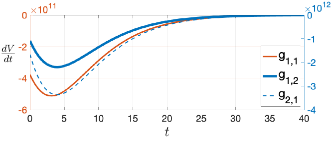
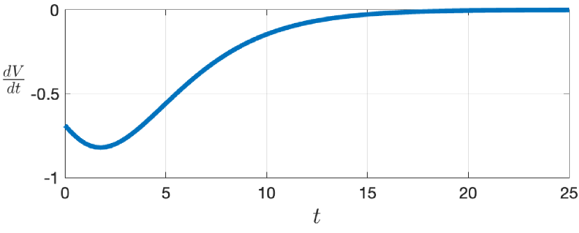
To determine the temporal stability, we employ Lyapunov stability theorem that is based on the function ($V([R]_{i},[P]_{i})$) (from the Appendix Eq. 25) which satisfies the necessary conditions: $V\left([R]_{i},[P]_{i}\right)=0$ when $[R]_{i}=[R]_{i}^{*}$ and $[P]_{i}=[P]_{i}^{*}$; where $[R]_{i}^{*}$ and $[P]_{i}^{*}$ are RNA and protein concentration at the equilibrium. Additionally, $V\left([R]_{i},[P]_{i}\right)>0$ due to the quadratic nature of all terms. Finally, we consider the first derivative of Eq. 25 as given by Eq. 27, as the last condition to be satisfied for the stability of the gene-perceptron. Then, according to the Lyapunov’s theorem, if Eq. 27 is negative, the gene-perceptron is asymptotically stable and if Eq. 27 is less than or equal to zero, the gene-perceptron is Lyapunov stable (See Eq. 25 - 27 in the Appendix for the complete derivation). Since it is difficult to directly determine the sign of the derivative of the Lyapunov function in Eq. 27 (please see the Appendix), we illustrate the temporal fluctuation of Eq. 27 in Figure 5. This provides us the insights into the dynamic stability behavior of the gene-perceptron.

Figure 5: Temporal stability of a Gene-perceptron based on the derivative of the Lyapunov function with respect to time. This shows that the gene-perceptron reaching stability over time.

Gene Regulatory Neural Network Analysis

While the previous section present the stability analysis of each individual gene-perceptron, they need to be integrated into a GRNN in order to perform the classification operation. We focus on two types of generic multi-layer GRNNs. In the first network, we consider direct gene relationships within the GRN from the input to the outputs that mimics a multi-layer ANN. In the second case, we consider a Random structured multi-layer GRNN with intermediate gene-perceptrons.

Multi-layer GRNN

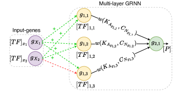
This GRNN network, which is illustrated in Figure 6, consists of three hidden layer gene-perceptrons ($g_{1,1},g_{1,2},g_{1,3}$) and one output layer gene-perceptron ($g_{2,1}$) ($g_{i,j}$ represents the $j^{\text{th}}$ gene-perceptron in $i^{\text{th}}$ layer in the sub-network). The concentrations that is output from layer 1 to layer 2 are $[TF]_{1,1},[TF]_{1,2},[TF]_{1,3}$ and $[P]$ is the output from gene-perceptron $g_{2,1}$. The two input-genes ($g_{X_{1}}$and $g_{X_{2}}$) are TFs with corresponding concentrations ($[TF]_{x_{1}}$ and $[TF]_{x_{2}}$), respectively. The RNA concentration change over time $t$, for the hidden layer gene-perceptrons, based on Eq. 1, can be expressed as,

$$\dfrac{d[R]_{i}}{dt}=k_{1_{i}}C_{N_{i}}\left(\dfrac{[TF]_{x_{1}}^{n}}{K_{A_{i}}^{n}+[TF]_{x_{1}}^{n}}\right)\cdot\left(\dfrac{[TF]_{x_{2}}^{n}}{K_{A_{i}}^{n}+[TF]_{x_{2}}^{n}}\right)-d_{1_{i}}[R]_{i},$$ (8)

for the activators, $i=g_{1,1},g_{1,2}$. Since the gene-perceptron $g_{1,3}$ has a repression from gene-perceptron $g_{x_{2}}$, the changes in the RNA production based on Eq. 3, is given by

$$\dfrac{d[R]_{g_{1,3}}}{dt}=k_{1_{g_{1,3}}}C_{N_{g_{1,3}}}\left(\dfrac{[TF]_{x_{1}}^{n}}{K_{A_{g_{1,3}}}^{n}+[TF]_{x_{1}}^{n}}\cdot\dfrac{K_{A_{g_{1,3}}}}{K_{A_{g_{1,3}}}+[TF]_{x_{2}}^{n}}\right)\\ -d_{1_{g_{1,3}}}[R]_{g_{1,3}}.$$ (9)

The RNA concentration changes of the output gene-perceptron $g_{2,1}$ that consists of TFs from the gene-perceptrons $g_{1,1},g_{1,2}$ and $g_{1,3}$ with the output protein concentration that contribute as TF concentration ($[TF]_{1,1}=[P]_{g_{1,1}},[TF]_{1,2}=[P]_{g_{1,2}}$ and $[TF]_{1,3}=[P]_{g_{1,3}}$) to accumulate in order to invoke the expression is given by,

$$\dfrac{d[R]_{g_{2,1}}}{dt}=k_{1_{g_{2,1}}}C_{N_{g_{2,1}}}\left(\dfrac{[TF]_{1,1}^{n}}{K_{A_{g_{2,1}}}^{n}+[TF]_{1,1}^{n}}\right)\\ \cdot\left(\dfrac{[TF]_{1,2}^{n}}{K_{A_{g_{2,1}}}^{n}+[TF]_{1,2}^{n}}\right)\cdot\left(\dfrac{[TF]_{1,3}^{n}}{K_{A_{g_{2,1}}}^{n}+[TF]_{1,3}^{n}}\right)-d_{1_{g_{2,1}}}[R]_{g_{2,1}}.$$ (10)

Figure 6: Multi-layer GRNN with two-input layer nodes, three hidden-layer gene-perceptrons ($g_{1,1},g_{1,2},g_{1,3}$) and one output layer gene-perceptron ($g_{2,1}$) and their corresponding output concentrations are transcription factors $[TF]_{1,1},[TF]_{1,2},[TF]_{1,3}$ and protein concentration $[P]$ respectively. There are two input-genes ($g_{x_{1}}$, $g_{x_{2}}$) considered as two TFs with concentration of $[TF]_{x_{1}}$ and $[TF]_{x_{2}}$, respectively. In this context, $g_{i,j}$ represents the $j^{\text{th}}$ gene-perceptron in $i^{\text{th}}$ layer in the GRNN. Input-gene activators and input-gene repressors are denoted by $(+)$ and $(-)$ edges, respectively. The weights ($w$) of this GRNN is a function of the TF concentration corresponding to the half-maximal RNA concentration ($K_{A_{i}}$) and gene-product copy number ($C_{N_{i}}$) for the gene-perceptron $i$ represented as $w(K_{A_{i}},C_{N_{i}})$.

Each of the gene-perceptron also undergoes a translation process. Therefore, the protein concentration change for each gene-perceptron can be modelled using Eq. 4 for $i=g_{1,1},g_{1,2},g_{1,3}$ and $g_{2,1}$. The maximum-stable protein concentration can be derived by setting Eq. 8 -10 to zero to find $[R]_{i}^{*}$, which is then plugged into Eq. 4 and set to zero for $i=g_{1,1},g_{1,2},g_{1,3}$ and $g_{2,1}$, respectively.

$$i=g_{1,1},g_{1,2}\Longrightarrow[P]_{i}^{*}=\dfrac{k_{1_{i}}k_{2_{i}}C_{N_{i}}}{d_{1_{i}}d_{2_{i}}}\left(\dfrac{[TF]_{x_{1}}^{n}}{K_{A_{i}}^{n}+[TF]_{x_{1}}^{n}}\right)$$

$$\times\left(\dfrac{[TF]_{x_{2}}^{n}}{K_{A_{i}}^{n}+[TF]_{x_{2}}^{n}}\right),$$ (11)

$$[P]_{g_{1,3}}^{*}=\dfrac{k_{1_{g_{1,3}}}k_{2_{g_{1,3}}}C_{N_{g_{1,3}}}}{d_{1_{g_{1,3}}}d_{2_{g_{1,3}}}}\left(\dfrac{[TF]_{x_{1}}^{n}}{K_{A_{g_{1,3}}}^{n}+[TF]_{x_{1}}^{n}}\right)$$

$$\times\left(\dfrac{K_{A_{g_{1,3}}}}{K_{A_{g_{1,3}}}+[TF]_{x_{2}}^{n}}\right),$$ (12)

$$[P]_{g_{2,1}}^{*}=\dfrac{k_{1_{g_{2,1}}}k_{2_{g_{2,1}}}C_{N_{g_{2,1}}}}{d_{1_{g_{2,1}}}d_{2_{g_{2,1}}}}\left(\dfrac{[TF]_{1,1}^{n}}{K_{A_{g_{2,1}}}^{n}+[TF]_{1,1}^{n}}\right)$$

$$\times\left(\dfrac{[TF]_{1,2}^{n}}{K_{A_{g_{2,1}}}^{n}+[TF]_{1,2}^{n}}\right)\left(\dfrac{[TF]_{1,3}^{n}}{K_{A_{g_{2,1}}}^{n}+[TF]_{1,3}^{n}}\right).$$ (13)

Eq. 11 - 13, which are the stable concentration quantity of proteins produced, is used to compute the classification areas for each gene-perceptron based on the value of concentration, which is further elaborated in the Results section as we present a case study. Subsequently, we apply the approach from the Methods Section to show the stability of the gene-perceptron in this GRNN. The overall stability of the GRNN based on the derived Lyapunov function of Eq. 27 (please see Appendix), which can be further expressed for $l$ number of TFs connected to a gene-perceptron ($i$), is represented as follows

$$\frac{dV}{dt}=-\prod_{j=1}^{l}\frac{C_{N_{i}}^{2}\cdot[TF]_{j}^{2n}\cdot k_{1_{i}}^{2}\cdot e^{(-2t(d_{1_{i}}+d_{2_{i}}))}}{d_{1_{i}}d_{2_{i}}([TF]_{j}^{n}+K_{A_{j}}^{n})^{2}(d_{1_{i}}-d_{2_{i}})^{2}}\\ \times(d_{2_{i}}^{3}\cdot e^{(2d_{2_{i}}t)}-2d_{1_{i}}d_{2_{i}}^{2}\cdot e^{(2d_{2_{i}}t)}+d_{1_{i}}^{2}d_{2_{i}}\cdot e^{(2d_{2_{i}}t)})\\ +(d_{1_{i}}k_{2_{i}}^{2}\cdot e^{(2d_{1_{i}}t)}+d_{2_{i}}k_{2_{i}}^{2}\cdot e^{(2d_{2_{i}}t)})-\\ -(d_{1_{i}}k_{2_{i}}^{2}\cdot e^{(t(d_{1_{i}}+d_{2_{i}}))}+d_{2_{i}}k_{2_{i}}^{2}\cdot e^{(t(d_{1_{i}}+d_{2_{i}}))}),$$ (14)

where $[TF]_{j}$ and $K_{A_{j}}$ are concentration of $j^{\text{th}}$ TF and corresponding half maximal RNA concentration for gene-perceptron $i$, respectively.

Table 1: Parameter Configuration for the generic multi-layer GRNN in Fig. 6

Parameter	$C_{N_{g_{1,1}}}$	$C_{N_{g_{1,2}}}$	$C_{N_{g_{1,3}}}$	$C_{N_{g_{2,1}}}$	$k_{1_{g_{1,1}}}$	$k_{1_{g_{1,2}}}$	$k_{1_{g_{1,3}}}$	$k_{1_{g_{2,1}}}$	$k_{2_{g_{1,1}}}$	$k_{2_{g_{1,2}}}$	$k_{2_{g_{1,3}}}$	$k_{2_{g_{2,1}}}$
	$d_{1_{g_{1,1}}}$	$d_{1_{g_{1,2}}}$	$d_{1_{g_{1,3}}}$	$d_{1_{g_{2,1}}}$	$d_{2_{g_{1,1}}}$	$d_{2_{g_{1,2}}}$	$d_{2_{g_{1,3}}}$	$d_{2_{g_{2,1}}}$	$K_{A_{g_{1,1}}}(\times 10^{-7})$	$K_{A_{g_{1,2}}}(\times 10^{-7})$	$K_{A_{g_{1,3}}}(\times 10^{-7})$	$K_{A_{g_{2,1}}}(\times 10^{-7})$
Parameter set 1	100	250	500	400	0.1	0.2	0.4	0.5	0.1	0.2	0.4	0.5
	0.3	0.2	0.5	0.6	0.3	0.2	0.5	0.6	500	100	1000	50
Parameter set 2	1	2	5	6	0.1	0.2	0.4	0.5	0.1	0.2	0.4	0.5
	0.3	0.2	0.5	0.6	0.3	0.2	0.5	0.6	$100^{*}$	$20^{*}$	$10^{*}$	$50^{*}$

Table 2: Parameter configuration for the Random Structured GRNN in Figure 7.

Parameter	$k_{1_{g_{1,1}}}$	$k_{1_{g_{1,2}}}$	$k_{1_{g_{1,3}}}$	$k_{1_{g_{2,1}}}$	$k_{1_{g_{3,1}}}$	$k_{2_{g_{1,1}}}$	$k_{2_{g_{1,2}}}$	$k_{2_{g_{1,3}}}$	$k_{2_{g_{2,1}}}$	$k_{2_{g_{3,1}}}$
	$d_{1_{g_{1,1}}}$	$d_{1_{g_{1,2}}}$	$d_{1_{g_{1,3}}}$	$d_{1_{g_{2,1}}}$	$d_{1_{g_{3,1}}}$	$d_{2_{g_{1,1}}}$	$d_{2_{g_{1,2}}}$	$d_{2_{g_{1,3}}}$	$d_{2_{g_{2,1}}}$	$d_{2_{g_{3,1}}}$
	$C_{N_{g_{1,1}}}$	$C_{N_{g_{1,2}}}$	$C_{N_{g_{1,3}}}$	$C_{N_{g_{2,1}}}$	$C_{N_{g_{3,1}}}$	$K_{A_{g_{1,1}}}(\times 10^{-7})$	$K_{A_{g_{1,2}}}(\times 10^{-7})$	$K_{A_{g_{1,3}}}(\times 10^{-7})$	$K_{A_{g_{2,1}}}(\times 10^{-7})$	$K_{A_{g_{3,1}}}(\times 10^{-7})$
Parameter set 1	0.1	0.2	0.4	0.8	0.5	0.1	0.2	0.4	0.7	0.5
	0.3	0.2	0.5	0.7	0.6	0.3	0.2	0.5	0.9	0.6
	1	2	5	10	6	500	100	1000	50	50
Parameter set 2	0.1	0.2	0.4	0.8	0.5	0.1	0.2	0.4	0.7	0.5
	0.3	0.2	0.5	0.7	0.6	0.3	0.2	0.5	0.9	0.6
	1	2	5	10	6	$50^{*}$	$100^{*}$	$1000^{*}$	$10^{*}$	$50^{*}$

Note: The values marked with an asterisk (*) are the parameters that are modified. Units of $C_{N_{i}},k_{1_{i}},k_{2_{i}},d_{1_{i}},d_{2_{i}}$ and $K_{A_{i}}$ are $molecules,\;sec^{-1},sec^{-1},min^{-1},hour^{-1}$ and $molecules$ respectively for both tables (Table 1 and 2).

Random Structured GRNN

As described earlier, relationship of gene-perceptrons within a GRN that have common TFs may have intermediate gene-perceptrons within the path of connections. We analyze how this impacts on the overall stability of the GRNN, where the network for this case is presented in Figure 7. In this form of networks, it is necessary to consider the RNA concentration change from the intermediate gene-perceptron ($g_{2,1}$) and its impact on the output layer gene-perceptron ($g_{3,1}$). The expressions for each gene-perceptrons, and their relative TFs from their immediate predecessor, is represented as follows:

$$\dfrac{d[R]_{g_{2,1}}}{dt}=k_{1_{g_{2,1}}}C_{N_{g_{2,1}}}\left(\dfrac{[TF]_{1,1}^{n}}{K_{A_{g_{2,1}}}^{n}+[TF]_{1,1}^{n}}\right)-d_{1_{g_{2,1}}}[R]_{g_{2,1}},$$ (15)

$$\dfrac{d[R]_{g_{3,1}}}{dt}=k_{1_{g_{3,1}}}C_{N_{g_{3,1}}}\left(\dfrac{[TF]_{2,1}^{n}}{K_{A_{g_{3,1}}}^{n}+[TF]_{2,1}^{n}}\right)\cdot\left(\dfrac{[TF]_{1,2}^{n}}{K_{A_{g_{3,1}}}^{n}+[TF]_{1,2}^{n}}\right)$$

$$\times\left(\dfrac{[TF]_{1,3}^{n}}{K_{A_{g_{3,1}}}^{n}+[TF]_{1,3}^{n}}\right)-d_{1_{g_{3,1}}}[R]_{g_{3,1}}.$$ (16)

Figure 7: Random structured GRNN with 3 input-layer gene-perceptrons ($g_{1,1},g_{1,2},g_{1,3}$), one intermediate gene-perceptron ($g_{2,1}$) and one output layer gene-perceptron ($g_{3,1}$). This structure is an extension from the GRNN in Figure 6.

Here, the protein concentration from Eq. 5 can be derived from Eq. 15 (i.e., $[TF]_{1,1}=[P]_{1,1}$), since the gene-perceptron $g_{2,1}$ is activated by gene-perceptron $g_{1,1}$. The RNA concentration models behaves similarly to the case without the intermediate gene-perceptron for the gene-perceptrons $g_{1,1},g_{1,2}$ $g_{1,3}$ and can be derived directly from Eq. 8 and 9. Using Eq. 4 we can determine the protein concentration change for each gene-perceptron Figure 7.

Using the maximum-stable protein concentration derived from Eq. 15 and 16, we can determine $[R]_{i}^{*}$, which is then applied to Eq. 4 and used to determine the maximum-stable value for $i=g_{2,1}$ and $g_{3,1}$. This will result in the following maximum-stable protein production that is represented as follows

$$[P]^{*}_{g_{2,1}}=\dfrac{k_{1_{g_{2,1}}}k_{2_{g_{2,1}}}C_{N_{g_{2,1}}}}{d_{1_{g_{2,1}}}d_{2_{g_{2,1}}}}\left(\dfrac{[TF]_{1,1}^{n}}{K_{A_{g_{2,1}}}^{n}+[TF]_{1,1}^{n}}\right),$$ (17)

$$[P]^{*}_{g_{3,1}}=\dfrac{k_{1_{g_{3,1}}}k_{2_{g_{3,1}}}C_{N_{g_{3,1}}}}{d_{1_{g_{3,1}}}d_{2_{g_{3,1}}}}\left(\dfrac{[TF]_{2,1}^{n}}{K_{A_{g_{3,1}}}^{n}+[TF]_{2,1}^{n}}\right)$$

$$\cdot\left(\dfrac{[TF]_{1,2}^{n}}{K_{A_{g_{3,1}}}^{n}+[TF]_{1,2}^{n}}\right)\left(\dfrac{[TF]_{1,3}^{n}}{K_{A_{g_{3,1}}}^{n}+[TF]_{1,3}^{n}}\right).$$ (18)

We use Eq. 11 to determine $[P]^{*}_{i}$ for $i=g_{1,1}$ and $g_{1,2}$, while for $i=g_{1,3}$ we use Eq. 12. For the stability analysis, Eq. 14 is used with $l=2$ for $g_{1,1},g_{1,2}$ and $g_{1,3}$, $l=1$ for $g_{2,1}$ and $l=3$ for $g_{3,1}$ corresponding to the number of TFs for each gene-perceptron.

Results

In this section, we perform the temporal stability analysis and obtain the classification areas for the two multi-layer GRNN network topologies (Figures 6, 7) as well as the GRNN derived from E.Coli GRN.

Multi-layer GRNN

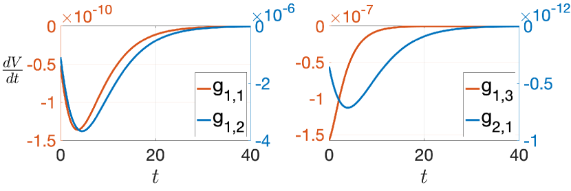
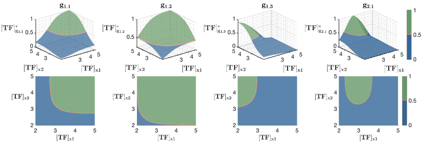
The temporal stability for each gene-perceptron within the generic multi-layer GRNN is illustrated in Figure 8. This simulation employed the model from Eq. 14 with the parameter set 1 (Table 1). Gene-perceptrons $g_{1,1}$ and $g_{1,2}$ initially move away from Lyapunov stability within 5 seconds, indicating a negative trend $\left(\frac{dV}{dt}<0\right)$ in the derivative of the Lyapunov function. However, after that it gradually achieved Lyapunov stability maintaining a positive trend and keeping the derivative of the Lyapunov function near zero $\left(\frac{dV}{dt}\approx 0\right)$. In contrast, the gene-perceptron $g_{1,3}$ exhibited positive trend from the beginning reaching Lyapunov stability within 15 seconds due to its distinct repression from the input-gene $g_{X_{1}}$. The output-layer gene-perceptron ($g_{2,1}$) followed a similar trend as gene-perceptrons $g_{1,1}$ and $g_{1,2}$ attaining Lyapunov stability within the initial 30 seconds because its immediate predecessors are all activators.

Figure 8: Temporal stability of the gene-perceptrons in the Multi-layer GRNN.

(a)

(b)

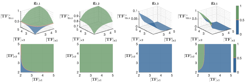
Figure 9: Parameter configurations for the Multi-layer GRNN depicted in Figure 6. Each graph depicts the classification area of each gene-perceptron and for (a) Parameter set 1, as well as (b) Parameter set 2 ($g_{2,1}$ is the output gene-perceptron that combines all classification areas of gene-perceptrons from the previous layer).

Given the gene-perceptron’s stability at the equilibrium (Figure 8), we can use Eq. 11 - 13 to calculate output protein $[P]_{i}^{*}$ for different input concetrations ($[TF]_{x_{1}}$ and $[TF]_{x_{2}}$). The calculated output protein $[P]_{i}^{*}$ is illustrated over varying input concentrations, highlighting the values above and below the threshold ($[P]^{*}=0.5$). Decision boundaries reflect how the classification areas change based on the edge (activation or repression) connected to the target gene-perceptron and corresponding parameters in Eq. 11 - 13. The inputs ($[TF]_{x_{1}}$ and $[TF]_{x_{2}}$) vary, while parameters like gene product copy number ($C_{N_{i}}$), transcription rate ($k_{1_{i}}$), translation rate ($k_{2_{i}}$), RNA degradation rate ($d_{1_{i}}$), protein degradation rate ($d_{2_{i}}$) and TF concentration corresponding to the half maximal RNA concentration ($K_{A_{i}}$) are kept constant. We consider two parameters sets to determine the different classification regions, which are presented in Table 1.

For the parameters set 1, we obtain the classification areas shown in Figure 9(a). The decision boundary and their top-view for each gene-perceptron are shown in the first and second row, respectively. The gene-perceptron $g_{1,2}$ has the largest classification area above the threshold due its lower TF concentration corresponding to half maximal RNA concentration $K_{A_{i}}$, compared to gene-perceptrons $g_{1,1}$ and $g_{1,3}$. Moreover, the decision boundaries for gene-perceptrons $g_{1,1}$ and $g_{1,2}$ exhibits a similar shape classifying majority of the values above the threshold. In contrast, the gene-perceptron $g_{1,3}$ covers larger area for the values below the threshold since it is repressed by the input-gene $g_{x_{2}}$. The intersection of classification areas corresponding to hidden layer gene-perceptrons is represented by the output layer gene-perceptron $g_{2,1}$, where the classification area above the threshold is approximately bounded by input concentrations, $2.5\leq[TF]_{x_{1}}\leq 3.5$ and $3.4\leq[TF]_{x_{2}}$. Due to the significant contribution from gene-perceptrons $g_{1,1}$ and $g_{1,2}$ beyond the threshold, the output layer gene-perceptron $g_{2,1}$ exhibits a rightward shift.

For the parameter set 2 (Table 1), the lower $K_{A_{i}}$ values have shifted the classification area above the threshold compared to parameter set 1. This shift is evident in Figure 9(b), particularly for the gene-perceptron $g_{1,2}$, which results in classifying majority of the values above the threshold. Conversely, for the gene-perceptron $g_{1,3}$, the classification area shifts below the threshold due to the repression from the input when reducing the half maximal RNA concentration $K_{A_{i}}$. The classification range for the gene-perceptron $g_{1,1}$ expands compared to parameter set 1, approximately bounded by $2.3\leq[TF]_{x,1}$ and $2.1\leq[TF]_{x,2}$. Considering all gene-perceptrons, the output layer gene-perceptron $g_{2,1}$ shows a leftward shift in the decision boundary, becoming slightly more linear. Overall, modifying the half maximal RNA concentration $K_{A_{i}}$ can significantly expand the classification area.

Random Structured GRNN

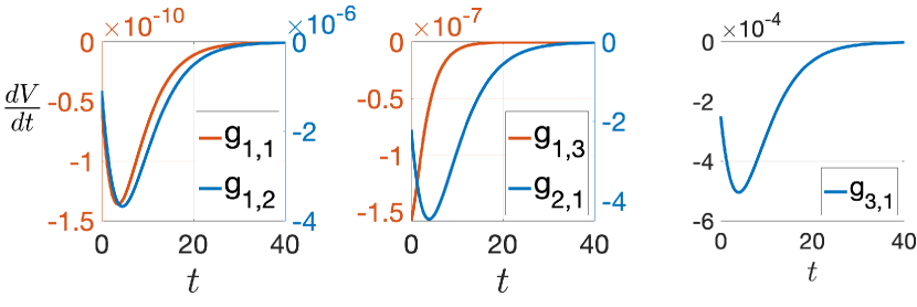
Figure 10: Temporal stability of the gene-perceptrons for the Random Structured GRNN.

Figure 11: Temporal stability for each gene-perceptrons in the E. coli GRNN.

This GRNN consists of three hidden layer gene-perceptrons, one intermediate gene-perceptron and one output layer gene-perceptron as illustrated in Figure 7. The temporal stability analysis for this GRNN is presented in Figure 10 and utilizes Eq. 14 and the parameter set 1 from Table 2. Similar to the Figure 8, gene-perceptrons $g_{1,1},g_{1,2},g_{3,1}$ and the intermediate gene-perceptron $g_{2,1}$ exhibit consistent stability fluctuations due to their immediate predecessor being activators. Additionally, gene-perceptron $g_{1,3}$ shows similar stability fluctuation patterns as the gene-perceptron $g_{1,3}$ in the network without the intermediate gene-perceptron and this is because both are being influenced by their repressive predecessors.

(a)

(b)

Figure 12: Parameter configurations for the Random Structured GRNN in Figure 6. Each graph depicts the classification area of each gene-perceptron and for (a) Parameter set 1; (b) Parameter set 2 ($g_{3,1}$ is the output gene-perceptron that combines all classification areas of gene-perceptrons from the previous layer).

Following the temporal stability analysis, we apply Eq. 11 and 12 to determine the maximum-stable protein concentration ($[P]^{*}_{i}$) for the gene-perceptrons $g_{1,1},g_{1,2}$ and $g_{1,3}$. However, unlike the GRNN in Figure 6, Eq. 13 is not used to determine the classification area for the output layer gene-perceptron. Instead, for the computation of $[P]^{*}_{i}$ for the gene-perceptrons $g_{2,1}$ and $g_{3,1}$, both Eq. 17 and 18 is employed due to the addition of the intermediate gene-perceptron compared to the multi-layer GRNN in Figure 6. The calculated protein concentration output $[P]^{*}_{i}$ values for different input concentrations used to determine the classification area for each gene-perceptron is presented in Figure 12. We also used two different sets of parameters from Table 2 to analyze different classification areas.

The parameter set 1 results in the classification areas shown in Figure 12(a). As the gene-perceptron $g_{2,1}$ serves as the intermediate gene-perceptron of $g_{1,1}$, we observe similar classification areas and decision boundaries. Additionally, repression from the input-gene $g_{x_{1}}$ to the gene-perceptron $g_{1,3}$ results in a distinctive decision boundary, approximately within the range of $3\leq[TF]_{x_{2}}$ and $3\geq[TF]_{x_{1}}$. Overall, the gene-perceptron $g_{3,1}$ represents the intersection of the hidden layer gene-perceptrons, with the classification area beyond the threshold bounded by $2.5\leq[TF]_{x_{2}}\leq 3.5$ and $3\geq[TF]_{x_{1}}$.

In contrast, reducing the TF concentration at the half maximal RNA concentration ($K_{A_{i}}$) for a gene-perceptron as shown in parameter set 2, alters the classification areas for both gene-perceptron $g_{1,1}$ and its immediate intermediate gene-perceptron $g_{2,1}$, as illustrated in Figure 12(b). The classification area significantly expands above the threshold, while dropping below it when lowering the TF concentration corresponding to the half-maximal RNA concentration $K_{A_{i}}$, as it is inversely proportional to the maximum protein concentration $[P]^{*}_{i}$ based on Eqs. 8 and 17. Alterations made to gene-perceptron $g_{1,1}$ notably impacts $g_{2,1}$, the predecessor gene-perceptron in the GRNN. Other hidden layer gene-perceptrons $g_{1,2}$ and $g_{1,3}$ remain unaffected between parameter sets 1 and 2. Parameter set 2 results in a leftward shift in the classification area of the output layer gene-perceptron $g_{3,1}$ compared to set 1. In summary, parameter adjustments leads to shifts in the decision boundary of the output layer gene-perceptrons; with decreased $K_{A_{i}}$ causing a leftward shift in the the classification area.

E.Coli GRNN Classification Analysis

(a)

(b)

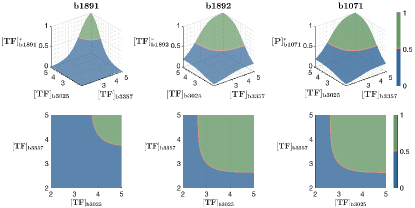
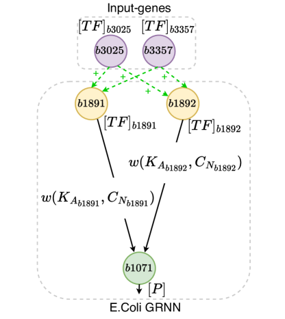
Figure 13: E. coli GRNN classification analysis. (a) Fully-connected GRNN derived from the E.coli GRN. This network consists of two input-genes ($b3025,b3357$), two hidden layer gene-perceptrons ($b1891$ and $b1892$), and one output layer gene-perceptron ($b1071$). (b) Classification regions of each gene perceptron within the E. coli GRNN, with gene-perceptron $b1071$ as the output.

This section demonstrates the classification areas for the E.coli GRNN illustrated in Figure 13(a), which is extracted from the trans-omic data of E.coli GRN (tierrafria2022regulondb). The network consists of two input-genes ($b3025,b3357$), two hidden layer gene-perceptrons ($b1891$ and $b1892$) and one output layer gene-perceptron ($b1071$) with their corresponding TF concentrations $[TF]_{i}$ for $i=b3025,b3357,b1891$ and $b1892$, and protein concentration $[P]_{b1071}$. In this specific GRNN, all TFs are considered activators. For the output layer gene-perceptron ($i=b1071$), we employ Eqs. 8, 4 and 11 with TFs $x_{1}=b1891$ and $x_{2}=b1892$ to calculate RNA, protein concentration change and maximum protein concentration ($[P]^{*}_{i}$), respectively using the parameter values in Table 3.

Similar to the previous GRNNs, we based the stability analysis for this GRNN on Eq. 14. For the 2 input layer gene-perceptrons ($i=b1891$ and $b1892$), we consider TFs $j=b3025,b3357$, while for the output layer gene-perceptron $i=b1071$, we evaluate stability with the TFs $j=b1891,b1891$ . In the previous GRNNs, we found that in Figures 8, 10 that the gene-perceptrons with an immediate activator, exhibits a consistent stability fluctuations before reaching Lyapunov stability $\left(\frac{dV}{dt}\approx 0\right)$. This is also a similar behaviour with the E.Coli GRNN, which is shown in Figure 11, which shows the temporal stability for the gene-perceptrons ($g_{1,1},g_{1,2}$ and $g_{2,1}$) that is influenced by the immediate activator predecessors displaying uniform stability. Overall, the analysis indicates that all the gene-perceptrons in the GRNN eventually attained the Lyapunov stability, ensuring network-wide stability, but with different timing periods.

Table 3: Parameter values used for the E.coli GRNN.

Parameter	Value			Ref.
	b1891	b1892	b1071
$k_{1_{i}}(sec^{-1})$	$0.05$	$0.05$	$0.05$	(milo2010bionumbers)
$k_{2_{i}}(sec^{-1})$	0.05	0.05	0.05	(gong2008comparative), (zhu2019maintenance)
$C_{N_{i}}(molecules)$	72	122	151	(keseler2017ecocyc)
$d_{1_{i}}(min^{-1})$	0.2	0.2	0.2	(milo2010bionumbers)
$d_{2_{i}}(hour^{-1})$	$3.5\%$	$3.5\%$	$3.5\%$	(milo2010bionumbers)
$K_{A_{i}}\left(\times 10^{-7}\right)$	75.30 (b3025)	71.10 (b3025)	306 (b1891)	GSE65244
	4261.64 (b3357)	2061.56 (b3357)	377 (b1892)

Note: $K_{A_{i}}$ of the corresponding TF is given in the table.

Once proving the stability of the GRNN, we ascertain the maximum-stable protein concentration to obtain the classification ranges. In order to compute maximum-stable protein concentration ($[P]^{*}_{i}$) for gene-perceptrons $i=b1891$ and $1892$, we use Eq. 11 with the replacement of $x_{1}$ and $x_{2}$ by $b3025$ and $b3357$ as input genes. Furthermore, for the computation of output concentrations $[P]^{*}_{i}$, concerning gene-perceptron $i=b1071$, Eq. 11 is used with TFs as $x_{1}=b1891$ and $x_{2}=b1892$ with the assumption that the Hill coefficient $n$ is equal to 1 in all simulations. Since $K_{A_{i}}$ is the TF concentration corresponding to the half maximal RNA concentration, there are two $K_{A_{i}}$ values for each gene-perceptron because each has two TFs, as shown in Figure 13(a). The time-series data of gene expression levels for E.coli was used by first identifying the gene’s half maximal expression level $K_{A_{i}}$ and then finding the expression level of its TF at that corresponding time point. For the remaining parameters that was obtained from literature as shown in Table 3, the average value was used.

The classification area from our analysis is shown in Figure 13(b). The classification area of gene-perceptron $b1892$ has expanded towards the left when compared to $b1891$, and this is because the expression level of the half-maximal RNA concentration $K_{A_{i}}$ of both TFs ($b3025$ and $b3357$) corresponding to $b1891$ exceed the value of $K_{A_{i}}$ for $b1892$. The classification area above the threshold of $b1892$ is defined within the limits of $[TF]_{b3025}\geq 2.7$ and $[TF]_{b3357}\geq 2.7$, in contrast to $b1891$ which is approximately bounded by $[TF]_{b3025}\geq 3.5$ and $[TF]_{b3357}\geq 3.8$. Consistent with the decision boundary simulations performed on the two generic multi-layer GRNNs (Figure 9 and 12), the output-layer gene-perceptron ($b1071$) of this GRNN also exhibited a intersection of classification areas driven by the input-layer gene-perceptrons. In line with this, as gene-perceptron $b1891$ had the majority of its classification area below the threshold and gene-perceptron $b1892$ had the majority above the threshold, the decision boundary of gene-perceptron $b1071$ is approximately bounded by $[TF]_{b3025}\geq 2.9$ and $[TF]_{b3357}\geq 2.9$. Overall, gene-perceptrons within the GRNN derived from E.coli GRN exhibit tunable decision boundaries by selecting sub-netowrks from the GRN at steady-state and collectively they function as multi-layer GRNN showcasing aspects of biological AI.

Conclusion

In this study, we introduced a GRNN that can be derived from a cell’s GRN and mathematical modelling this for the transcription and translation process, transforming a gene into a gene-perceptron. We also performed stability analysis for the GRNN as it functions as a non-linear classifier. This is based on the eigenvalue method and the Lyapunov’s stability theorem, with the latter approach capable of determining the time at which the stability is achieved. The classification application was applied to two multi-layer GRNNs as well as a sub-network extracted from the E.coli GRN using trans-omic data. From the simulation for different parameter settings for the two multi-layer GRNN revealed that the TF concentration at the half maximal gene expression level $K_{A_{i}}$, has a significant impact on the shifting of the classification boundary. Based on the outcomes of the stability analysis and simulations, we can conclude that the GRN exhibits NN properties as the gene-perceptron demonstrated sigmoidal-like behavior for multiple inputs and tunable decision boundary. Further, by engineering living cells it is possible to obtain desired non-linear classifiers based on our application. Our model has potential to transform GRNs into GRNN when the suitable parameters are established for the dual-layered chemical reaction model.

Author contributions

A.R., S.S. and S.B. designed the theoretical framework of the study. The implementation of the analysis was done by A.R. while A.G. provided the knowledge for the biological aspect of this study. All the authors wrote and reviewed the final manuscript.

Declaration of interests

The authors declare no competing interests.

Appendix

RNA and Protein Concentration Model

To model the RNA and protein concentration change, mass-balance differential equations were used based on Hill function. Transcription of a gene-perceptron begins with TF and RNA polymerase binding to the promoter, which is modelled by,

$$[Prom.TF]=C_{N_{i}}\dfrac{[TF]^{n}}{[TF]^{n}+K_{A_{i}}^{n}},$$ (19)

where $[TF],n,K_{A_{i}},[Prom.TF]$ and $C_{N_{i}}$ are concentration of TFs, Hill coefficient, TF concentration corresponding to half maximal RNA concentration, complex produced after TFs bind to promoter and gene product copy number, respectively. The complex, $Prom.TF$ transcribes into RNA at the rate of $k_{1_{i}}$ and subsequently RNA degrades at the rate of $d_{1_{i}}$ which can be modelled as

$$\dfrac{d[R]_{i}}{dt}=k_{1_{i}}[Prom.TF]-d_{1_{i}}[R]_{i}.$$ (20)

By plugging Eq. 19 in Eq. 20 we can obtain Eq. 1. In contrast, if a gene-perceptron is repressed by a TF, Eq. 19 can be expressed as

$$[Prom.TF]=C_{N_{i}}\dfrac{K_{A_{i}}^{n}}{K_{A_{i}}^{n}+[TF]^{n}}.$$ (21)

Since the initial RNA concentration transcribed by a gene-perceptron is $[R]_{i}(0)$ (i.e., $[R]_{i}(t=0)=[R]_{i}(0)$), the solution of Eq. 1 as given by Eq. 2 can be derived using the integrating factor, $IF=e^{\int d_{1_{i}}\,dt}=e^{d_{1_{i}}t}$ , where $t$ and $d_{1_{i}}$ are time and RNA degradation rate, respectively. Transcribed RNA is then translated into protein at the proteome level. To solve the differential equation of protein concentration change for Eq. 4 we can follow 2 steps. Step 1: Replacing RNA concentration ($[R]_{i}$) in Eq. 4 with the solution obtained for the differential equation of RNA concentration change from Eq. 2. Step 2: Using the integrating factor ($IF=e^{\int d_{2_{i}}dt}=e^{d_{2_{i}}t}$) and initial RNA concentration ($[R]_{i}(0)$), as well as initial protein concentration $[P]_{i}(0)$ (i.e., $[P]_{i}(t=0)=[P]_{i}(0)$) we can obtain the equation for the protein concentration in Eq. 5. By setting $\dfrac{d\,[R]_{i}}{dt}=0$, we can obtain maximum-stable RNA concentration at the steady-state ($[R]_{i}^{*}$) expressed by Eq. 6. In addition, protein concentration at the steady-state ($[P]_{i}^{*}$) can be represented by Eq. 7 which is derived by plugging $\dfrac{d\,[P]_{i}}{dt}=0$ in Eq. 4.

Determining Gene-perceptron Stability

In this section, we derive the stability of a gene-perceptron using eigenvalues of differential equations for RNA and protein concentration change (Eq. 1 and 4) and using Lypunov’s stability theorem. Based on (samaniego2021signaling), we applied eigenvalue method to determine the stability in the gene-perceptrons. Suppose $f$ and $g$ are functions of $[R]_{i}$ and $[P]_{i}$. Such that,

$$\text{Eq.}\ref{eq:rna_activate}\Longrightarrow\dfrac{d\,[R]_{i}}{dt} =f\left([R]_{i},[P]_{i}\right),$$ (22)

$$\text{Eq.}\ref{eq: prot_change}\Longrightarrow\dfrac{d\,[P]_{i}}{dt} =g([R]_{i},[P]_{i}).$$ (23)

Then, the Jacobian matrix for Eqs. 1 and 4 at the equilibrium point is represented as,

$$J_{i}=\begin{bmatrix}\frac{\partial f}{\partial[R]_{i}}&\frac{\partial f}{\partial[P]_{i}}\\ \frac{\partial g}{\partial[R]_{i}}&\frac{\partial g}{\partial[P]_{i}}\end{bmatrix}=\begin{bmatrix}-d_{1_{i}}&0\\ k_{2_{i}}&-d_{2_{i}}\end{bmatrix},$$ (24)

for gene-perceptron $i$. Using the characteristic equation $|J_{i}-\lambda I|=0$ we can determine the eigenvalues for the above Jacobian matrix (Eq. 24) as $\lambda_{1}=-d_{1_{i}},\lambda_{2}=-d_{2_{i}}$. Hence, all the eigenvalues are negative, indicating that the gene-perceptron is stable, where $\lambda$ is scalar, $I$ is a $2\times 2$ identity matrix, $d_{2_{i}}$ is the protein degradation rate, $d_{1_{i}}$ is the RNA degradation rate and $k_{2_{i}}$ is the translation rate. We use the Lyapunov function ($V$) to perform the temporal stability analysis defined for the Eqs. 1 and 4 as follows,

$$V\left([R]_{i},[P]_{i}\right) =\left([R]_{i}-[R]_{i}^{*}\right)^{2}+\left([P]_{i}-[P]_{i}^{*}\right)^{2}.$$ (25)

According to the Lyapunov’s stability theorem, $V\left([R]_{i},[P]_{i}\right)=0$ when $[R]_{i}=[R]_{i}^{*}$ and $[P]_{i}=[P]_{i}^{*}$, where $[R]_{i}^{*}$ and $[P]_{i}^{*}$ are RNA and protein concentration at the equilibrium. It is clear that $V\left([R]_{i},[P]_{i}\right)>0$, since all terms are quadratic. Finally, we consider the first derivative of Eq. 25 as the last condition for the stability, which is represented as

$$\dot{V}([R]_{i},[P]_{i})=\dfrac{dV}{dt}=\frac{\partial V}{\partial[R]_{i}}.\dfrac{d[R]_{i}}{dt}+\frac{\partial V}{\partial[P]_{i}}.\dfrac{d[P]_{i}}{dt}.$$ (26)

By plugging $\frac{d[R]_{i}}{dt}$ and $\frac{d[P]_{i}}{dt}$ from Eq. 1 and 4, differentiating Eq. 25 with respect to $[R]_{i}$ and $[P]_{i}$ to obtain $\frac{\partial V}{\partial[R]_{i}}$ and $\frac{\partial V}{\partial[P]_{i}}$ and finally replacing $[R]_{i}^{*},[P]_{i}^{*},[R]_{i}$ and $[P]_{i},$ with Eq. 6, 7, 2 and 5 we get Eq. 26, which is represented as follows

$$\text{Eq.}\ref{eq: derivative_lyapunov}\Longrightarrow\frac{dV}{dt}=-\frac{C_{N_{i}}^{2}\cdot[TF]^{2n}\cdot k_{1_{i}}^{2}\cdot e^{(-2t(d_{1_{i}}+d_{2_{i}}))}}{d_{1_{i}}d_{2_{i}}([TF]^{n}+K_{A_{i}}^{n})^{2}(d_{1_{i}}-d_{2_{i}})^{2}}$$

$$\cdot(d_{2_{i}}^{3}\cdot e^{(2d_{2_{i}}t)}-2d_{1_{i}}d_{2_{i}}^{2}\cdot e^{(2d_{2_{i}}t)}+d_{1_{i}}^{2}d_{2_{i}}\cdot e^{(2d_{2_{i}}t)})$$

$$+(d_{1_{i}}k_{2_{i}}^{2}\cdot e^{(2d_{1_{i}}t)}+d_{2_{i}}k_{2_{i}}^{2}\cdot e^{(2d_{2_{i}}t)})$$

$$-(d_{1_{i}}k_{2_{i}}^{2}\cdot e^{(t(d_{1_{i}}+d_{2_{i}}))}+d_{2_{i}}k_{2_{i}}^{2}\cdot e^{(t(d_{1_{i}}+d_{2_{i}}))}),$$ (27)

where we assume initial RNA concentration of zero ($[R]_{i}(0)=0$) and initial protein concentration of zero ($[P]_{i}(0)=0$). The above equation is used to determine the stability of the gene-perceptron for different parameter configurations.