Investigating the Drivers of Electron Temperature Variations in HII Regions with Keck-KCWI and VLT-MUSE
Abstract
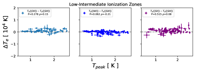
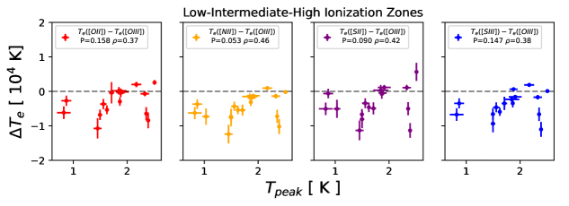
H ii region electron temperatures are a critical ingredient in metallicity determinations and recent observations reveal systematic variations in the temperatures measured using different ions. We present electron temperatures () measured using the optical auroral lines ([N II], [O II], [S II], [O III], and [S III]) for a sample of H ii regions in seven nearby galaxies. We use observations from the Physics at High Angular resolution in Nearby Galaxies survey (PHANGS) obtained with integral field spectrographs on Keck (Keck Cosmic Web Imager; KCWI) and the Very Large Telescope (Multi-Unit Spectroscopic Explorer; MUSE). We compare the different measurements with H ii region and interstellar medium environmental properties such as electron density, ionization parameter, molecular gas velocity dispersion, and stellar association/cluster mass and age obtained from PHANGS. We find that the temperatures from [O II] and [S II] are likely over-estimated due to the presence of electron density inhomogeneities in H ii regions. We observe that differences between [N II] and [S III] temperatures are weakly correlated with stellar association mass and molecular gas velocity dispersion. We measure high [O III] temperatures in a subset of regions with high molecular gas velocity dispersion and low ionization parameter, which may be explained by the presence of low-velocity shocks. Of all the temperatures considered, the – between [N II] and [S III] temperatures have the lowest observed scatter and generally follow predictions from photoionization modeling, which suggests that these tracers reflect H ii region temperatures across the various ionization zones better than [O II], [S II], and [O III].
1 Introduction
The characterization of abundance variations within galaxies provides insight into the physical processes that drive galaxy and chemical evolution. A galaxy’s gas-phase metal abundance (i.e., metallicity) reflects the history of chemical enrichment from stars and the net balance of gas flows (mixing, outflows, inflows of pristine material, etc.). In addition, the metallicity of ISM gas directly controls its cooling and other important ISM physics (Draine, 2011; Peimbert et al., 2017).
The distribution of gas-phase metals in a galaxy is commonly traced by the abundance of oxygen, nitrogen, sulfur, and other metals using the emission from ionized gas located inside H ii regions (e.g. Kennicutt & Garnett, 1996; Bresolin et al., 2012; Hernandez et al., 2013; Ho et al., 2017; Kreckel et al., 2019, 2020; van Loon et al., 2021; Grasha et al., 2022). There are several indirect methods calibrated using strong optical emission lines to derive an estimate of the H ii region metallicity (e.g. Kewley & Ellison, 2008; Blanc et al., 2015). A “direct” measure of an H ii region metallicity requires knowledge of the electron temperature () of the gas. Due to their exponential dependence on , one of the ways to infer electron temperature is through the auroral-to-nebular line ratios of collisionally excited lines (CEL; Peimbert, 1967; Osterbrock & Ferland, 2006; Peimbert et al., 2017). Nebular and auroral lines originate from different excited states of ions. Auroral lines are from higher energy levels, but are still accessible for collisional excitation in a K gas. If the density of the gas is below the auroral and nebular line critical densities (i.e. when collisional de-excitation is negligible), then the auroral-to-nebular line ratio is sensitive to the electron temperature (e.g., Osterbrock & Ferland, 2006). Given that the excitations to the auroral level are only accessible to electrons of higher energy, auroral line emission can be times weaker than nebular lines (Kennicutt et al., 2003; Esteban et al., 2004; Berg et al., 2020). One alternative way to to measure include the ratio between recombination line (RL) emission from H and other species, and which exhibit linear sensitivity to (Peimbert, 1967; Osterbrock & Ferland, 2006; Peimbert et al., 2017). However, optical RLs useful for use as temperature diagnostics are typically reserved for deep, high S/N spectra, as RL emission is typically much fainter than the emission from auroral lines.
For ions with optical auroral lines studied in this work, we can measure the temperatures for each ion using the following line ratios:
[O III]/,
[O II]/111[O II] is an unresolved quadruplet with transitions at , , and Å.,
[S III]/,
[S II]/,
[N II]/.
The O+, N+, S+ ions require energies of eV, eV, and eV to be produced while S++ and O++ require energies 23 eV and 35 eV, respectively.
Several effects play competing roles in determining the ionization and temperature structure of H ii regions. These include a radially decreasing intensity and hardening of the radiation field (photons closest to 13.6 eV are absorbed first) as well as a change in the ions which dominate gas cooling, and therefore the cooling efficiency (Stasińska, 1980; Garnett, 1992). Because of the varying degree of ionization within an H ii region, a model of three ionization zones—low-, intermediate- and high—is often used to describe them. Because each ionization zone could theoretically have different temperatures, this further stresses the importance of observing multiple auroral lines and developing temperature priorities for use in accurately determining abundances (e.g. Berg et al., 2015, 2020).
Observing the full set of optical auroral lines in an H ii region can be challenging. In addition to the large wavelength range needed, 3700–10000 Å, some auroral lines are weaker than others depending on the metallicity and temperature of the gas. Because of these challenges, it is very important to establish temperature relationships that allow us to infer the conditions of a certain ionization zone from the others. Photoionization modeling (e.g. Garnett, 1992; Vale Asari et al., 2016) has been used to derive temperature relationships, but standard models consider only simple geometries and homogeneous physical and ionization conditions, that might not be suitable for more complex regions potentially affected by shocks, stellar feedback or other mechanism that produce density or temperature inhomogeneities (Peimbert, 1967; Peimbert et al., 1991; Binette et al., 2012; Berg et al., 2015, 2020; Arellano-Córdova & Rodríguez, 2020; Nicholls et al., 2020; Méndez-Delgado et al., 2023b, a).
In the presence of temperature fluctuations, the exponential dependence of CEL strengths on temperature will bias auroral-to-nebular temperatures towards higher values than the true average (Peimbert, 1967; Peimbert & Costero, 1969). Such inhomogeneities may be related to the presence of turbulence, density structure, and shocks associated with either stellar winds or radiation–pressure driven expansion. If the sources of temperature inhomogeneities are confined to the central part of the nebula, the effects that these phenomena have on temperature may primarily affect only the high ionization zone. This has been suggested by Méndez-Delgado et al. (2023a) who presented evidence for temperature inhomogeneities affecting only the highly ionized gas traced by [O III]. In a sample of Galactic and extra-galactic H ii regions, they observed that differences between [O III] and [N II] temperatures correlated with the degree of deviation from the average temperature measured using faint O II recombination line emission. Furthermore, a strong correlation between the O II recombination and [N II] temperatures observed by Méndez-Delgado et al. (2023a) implies that temperatures inferred from the [N II] auroral line accurately measures the average of the low-ionization zone (Méndez-Delgado et al., 2023a, b).
Due to the importance of obtaining accurate temperatures for precise abundances, significant effort has been devoted to advancing our understanding of the temperatures of different H ii region ionization zones. For example, previous works have found that the scatter between temperatures of different ionization zones may be correlated with other properties of the gas such as the ionization parameter and metallicity (Berg et al., 2015; Arellano-Córdova & Rodríguez, 2020; Berg et al., 2020; Yates et al., 2020).
A number of important questions about electron temperatures in H ii regions remain. Past studies (e.g. Kennicutt et al., 2003; Rosolowsky & Simon, 2008; Berg et al., 2015, 2020; Wei et al., 2020) have typically targeted the brightest H ii regions in order to maximize the probability of detection of auroral lines. This procedure, however, may have introduced selection biases towards the brightest regions or those with particular physical conditions. In addition, due to observational challenges (e.g., wide wavelength range needed to cover the [S III] lines) it remains uncertain how temperature inhomogeneities may impact the intermediate ionization zone temperatures traced by [S III] (Méndez-Delgado et al., 2023b).
To explore these questions, we use deep 3600–9500 Å IFU mapping to measure the set of optical auroral lines and nebular lines for a sample of H ii regions. We use observations obtained from the Keck Cosmic Web Imager (KCWI, Morrissey et al., 2018) and Multi-Unit Spectroscopic Explorer (MUSE, Bacon et al., 2010) to measure the electron temperature from all 3 ionization zones in H ii regions in nearby galaxies. In Section 2 we present our sample galaxies as well as primary and supplemental observations. In Section 3 we discuss the reduction of the KCWI data. We assess the quality of the KCWI mosaics in Section 1. We construct our H ii region sample in Section 4. We present the auroral line measurements in Section 5. We derive H ii region properties from nebular diagnostics and from ALMA and HST data in Section 6. The results and discussion are presented in Section 7 and 8.
2 Observations
The analysis presented here makes joint use of multi-wavelength observations of seven galaxies obtained with Keck-KCWI, VLT-MUSE, Atacama Large Millimeter/submillimeter Array (ALMA), and the Hubble Space Telescope (HST).
2.1 Sample Selection
The seven galaxies in this analysis are drawn from the PHANGS-MUSE sample (Emsellem et al., 2022). To date, 90 galaxies make up the full PHANGS sample222http://phangs.org/ (Leroy et al., 2021a), and 19 have been observed by MUSE. In order to be observed with KCWI in the northern hemisphere, we selected the seven target galaxies from a subset of PHANGS-MUSE galaxies with declination, . Table 1 presents general properties of these galaxies, including distances, masses, sizes, and the angular resolution of the MUSE data.
2.2 Keck Cosmic Web Imager
We observed each galaxy using KCWI on the Keck II telescope with multiple pointings taken over several nights between the years 2017 and 2021. Clear conditions were present for the majority of observations, except for the nights of October 16 and 17, 2018, which suffered from variable cloud coverage. These poor conditions primarily affect the observations of NGC 628. The instrument was configured with the “Large” slicer and BL grating centered at 4600 Å. The usable spectral range afforded by this configuration is 3650–5550 Å with a spectral resolution , corresponding to a full width at half maximum (FWHM) Å (or 300 km s-1) at the central wavelength. The Large slicer has an angular slice width of 1.35″. The field of view (FoV) using the Large slicer and BL grating is 33″ perpendicular and 20.4″ parallel to the slicer.
Because the FoV is small compared with the large angular size of each galaxy, we observed each galaxy over multiple fields. Most fields were observed two times using 1200 s (i.e., 20 min) integration times. The only exceptions were: all fields in NGC 3627, which were observed five times each with 120 s (2 min) integration times; field 17 in NGC 628 which was observed 3 times using 1200 s; and field 2 in NGC 5068 and field 5 in NGC 1385, both having only a single observation of 1200 s. A half slice width, or 0.675″, dither was applied between each exposure. Immediately following the second exposure, we observed an off-galaxy region, selected to be free of extended emission and/or bright sources, in order to measure a sky spectrum close in time to the observations. These sky frames were used for sky subtraction during data reduction. We summarize the number of fields, exposure times, and dates in Table 7 of Appendix A. The full data reduction is outlined in Section 3.
2.3 Multi-Unit Spectroscopic Explorer
MUSE observations of these galaxies come from the PHANGS-MUSE survey (Emsellem et al., 2022). MUSE covers wavelengths between 4800–9500 Å. Taken in combination KCWI and MUSE span the full optical spectrum. The full details of the MUSE data reduction and data products are presented in Emsellem et al. (2022), and we provide a brief overview here. The PHANGS-MUSE program observed 19 galaxies using 168 individual 1 pointings. The median spatial resolution across all pointings is pc (or 0.80″) with a typical spectral FWHM of Å (but varying with wavelength). The data were reduced using the pymusepipe333https://pypi.org/project/pymusepipe/ and spectral fitting and analysis was performed using the Data Analysis Pipeline 444https://gitlab.com/francbelf/ifu-pipeline packages described in Emsellem et al. (2022). The individual MUSE pointings were homogenized to a uniform Gaussian point-spread-function (PSF) with FWHM set to the largest FWHM measured for each target, resulting in “convolved and optimized” (COPT) mosaics. The PSFs of the COPT mosaics are listed in Table 1. We use the COPT mosaics in the following work.
2.4 ALMA
Our analysis makes use of Atacama Large Millimeter/submillimeter Array (ALMA) data obtained as part of PHANGS–ALMA (Leroy et al., 2021a). PHANGS-ALMA observed the rotational transition of 12CO, hereafter CO, for galaxies. The details of the data reduction are described in Leroy et al. (2021b). We make use of the ALMA datacubes with combined CO measurements from the 12m and 7m arrays plus Total Power (12m+7m+TP). The nominal angular resolution of 12m+7m+TP observations is , similar to the resolution of both KCWI and MUSE. The velocity resolution is km s-1.
2.5 HST
The PHANGS-HST survey (Lee et al., 2022) observed555Lee et al. (2022) use of previous NGC 628 HST imaging obtained as part of the Legacy ExtraGalactic Ultraviolet Survey (Legus; Calzetti et al., 2015). our target galaxies using 5 HST filters: F275W (NUV), F336W (U), F438W (B), F555W (V), F814W (I). Of the high-level data products produced from this dataset, we make use of compact star cluster catalogs (Thilker et al., 2022) and multi-scale stellar association catalogs (Larson et al., 2023). The association catalog identifies sources using both the V and NUV filters and has been convolved to several physical resolutions (8, 16, 32 and 64 pc, respectively). Following Scheuermann et al. (2023) we used the NUV selected, 32 pc catalogs.
| Name | DistanceaaFrom the compilation of Anand et al. (2021) | log bbDerived by Leroy et al. (2021a), using GALEX UV and WISE IR photometry. | ccFrom LEDA Makarov et al. (2014). | PSFMUSEddThe FWHM of the Gaussian PSF for the homogenized COPT mosaic from PHANGS-MUSE (Emsellem et al., 2022). | PSFKCWIeeThe average FWHM of the KCWI PSF for the set of a galaxy’s observed pointings. | ||
|---|---|---|---|---|---|---|---|
| [Mpc] | [] | [Arcmin] | [Arcsec] | [Arcsec] | |||
| NGC 628 | 9\@alignment@align.80 | 10.340.1 | 4\@alignment@align.9 | 0.92 | 2\@alignment@align.0 0 | ||
| NGC 1087 | 15\@alignment@align.92 | 9.930.1 | 1\@alignment@align.5 | 0.92 | 1\@alignment@align.2 0 | ||
| NGC 1300 | 19\@alignment@align.02 | 10.620.1 | 3\@alignment@align.0 | 0.89* | 1\@alignment@align.3 0 | ||
| NGC 1385 | 17\@alignment@align.22 | 9.980.1 | 1\@alignment@align.7 | 0.77* | 1\@alignment@align.3 0 | ||
| NGC 2835 | 12\@alignment@align.20 | 10.000.1 | 3\@alignment@align.2 | 1.15 | 1\@alignment@align.4 0 | ||
| NGC 3627 | 11\@alignment@align.30 | 10.830.1 | 5\@alignment@align.1 | 1.05 | 1\@alignment@align.1 0 | ||
| NGC 5068 | 5\@alignment@align.20 | 9.400.1 | 3\@alignment@align.7 | 1.04 | 1\@alignment@align.5 0 | ||
3 KCWI Data Reduction
The KCWI observations were reduced using the Version 1.0.1 Python implementation of the KCWI Data Extraction and Reduction Pipeline (KDRP)666KCWI DRP-Python. It was built using the Keck Data Reduction Pipeline Framework package777KeckDRPFramework and is a port of the initial IDL reduction pipeline888KCWI DRP-IDL (Morrissey et al., 2018). The pipeline performs basic CCD reduction including bias and over-scan subtraction, gain correction, cosmic ray removal, dark and scattered light subtraction as well as a flat field correction.
Following these basic reductions, the KDRP used the continuum bar and Thorium/Argon arc lamp images to generate geometric and wavelength solutions to convert each 2D science image into a spectral datacube. The accuracy of the wavelength solutions were similar across all the observation nights. The average RMS for the derived wavelength solutions was 0.1 Å.
We derived an inverse sensitivity curve to flux calibrate each datacube from standard star observations. The measured standard deviation between all of the derived inverse sensitivity curves was at Å. The maximum standard deviation within the wavelength range containing the lines used in this analysis is . Details of each standard star observation can be found in Table 8 of Appendix A. After flux calibration, each datacube was corrected for differential atmospheric refraction.
Because the instrument FoV is much smaller than each galaxy, our images contained no sky pixels. To perform sky subtraction, we observed dedicated sky positions interspersed between science observations. We assigned the sky frame closest in time to each science observation to be used for sky subtraction according to the instructions in the KDRP documentation999https://kcwi-drp.readthedocs.io/en/latest/sky_subtraction.html. The KDRP then performed sky subtraction using our preferred frames. The sky in all pixels was averaged together and scaled by the ratio of science-to-sky exposure time to estimate the sky observed in the “on” position. The final data products output by the pipeline include flux calibrated science and uncertainty cubes, as well as a bad-pixel mask cube.
3.1 Image Re-Projection
Next we constructed mosaics from the individual KCWI pointing datacubes. The steps involved included image registration, matching the flux calibration to MUSE, and image co-addition. We also compared the absolute flux calibration of the final KCWI mosaics to MUSE and SDSS
The datacubes output by the KDRP have rectangular pixels with pixel-scale 1.35″ 0.29″. We reprojected the cubes onto a square pixel grid using the astronomical mosaic software Montage101010See http://montage.ipac.caltech.edu/. Prior to running Montage, we converted the KCWI data to surface brightness units (erg s-1 cm-2 Å-1 sr-1) by dividing the flux per pixel by the pixel solid angle in steradians. The reprojected images have a final square pixel grid with a uniform pixel-scale of 0.29″ 0.29″. We validated the flux-conservation in our data before and after reprojection.
3.2 Image Registration
To co-add each galaxy’s set of cubes into a spectral mosaic, we placed each cube onto a common world coordinate system (WCS). It is typical to perform image registration by matching the location of foreground stars or background galaxies to known positions found in catalogs. However, in our case most individual fields did not contain a sufficient number of bright point sources. Instead, we performed image registration by maximizing the cross-correlation between individual KCWI fields and overlapping MUSE data in order to match the KCWI pointing astrometry to MUSE. The astrometry of the MUSE galaxy mosaics were validated against wide-field broadband imaging and stellar positions from the Gaia DR1 as described in Emsellem et al. (2022). The MUSE astrometry, when compared to broadband imaging, exhibited better than 100 milli-arcseconds RMS. in both R.A. and Dec.
To cross-correlate KCWI and MUSE, we created synthetic photometry () images from spectral regions where the wavelength coverage of KCWI and MUSE overlap. Because there is some saturation in H and [O III] at the brightest locations in the KCWI data, we masked out those lines in both cubes to avoid any issues with the comparison between the two data cubes.
In order to determine the optimal astrometric shifts to apply to each KCWI science frame, we utilized a two-step grid search operation, first shifting in 1 pixel (or 0.29″) steps 17 pixels (or ) from the center of the KCWI pointing in order to find the optimal R.A. and Dec. offsets which maximize the correlation of the KCWI and corresponding MUSE images. After locating 1st-pass shifts, we performed a secondary grid search using finer 1/2 pixel increments over a smaller range ( from the image center). The 0.5 pixel sampling corresponds to 0.145″ which is less than the MUSE pixel scale of 0.20″ but also corresponds to 1/10 the typical KCWI FWHM which is equal to 1.2″. Across the galaxy sample, the final offsets correspond to correlation coefficients 0.9 between KCWI and MUSE.
3.3 Matching the MUSE Flux Calibration
In order to correct for any additive and/or multiplicative offsets between the MUSE and KCWI flux calibrations, we compared the surface brightness (SB) calculated in apertures in overlapping position and wavelength. To do this we made use of the images, described in Section 3.2, and measured the surface brightness inside a number of 3″ radius apertures located at randomly drawn positions inside the combined KCWI and MUSE coverage. The aperture size was chosen to be large enough to minimize effects arising from the different PSFs of KCWI and MUSE. We determined the best fit line to the measured vs. relationship, where the slope, , and -intercept, , reflect the multiplicative and additive offset between the KCWI and MUSE flux calibration. We applied the correction by multiplying the KCWI datacubes by and adding to the full spectrum in each pixel. The average multiplicative and additive offsets were and . This deviation from a 1–1 slope and low level of additive offset show that the calibrations were already in good agreement.
3.4 PSF of Individual KCWI Fields
Because the MUSE mosaics have been homogenized to a uniform Gaussian PSF, we have an image with a known (parameterized) PSF. This is advantageous, as we can directly measure the KCWI PSF per pointing using cross-convolution, following the steps outlined in Emsellem et al. (2022). We briefly summarize the procedure here. 1) We produced images of both the MUSE mosaic and the individual KCWI pointings. 2) We re-projected the MUSE cutout onto the KCWI 0.29″ 0.29″ pixel grid. 3) We convolved the KCWI pointing with a 2D Gaussian Kernel with PSF equal to the reference MUSE PSF. 4) In an iterative manner, the reference MUSE image is then convolved with a 2D Gaussian Kernel, PSFk, where the PSFk represents the KCWI pointing PSF which is a free-parameter. We then varied the FWHM of this kernel until we maximized the correlation between the KCWI pointing and the reference MUSE image. For the set of images observed for each galaxy, we present the average and standard deviation of the measured PSFs in Table 1. The average PSF across the galaxy sample is which is consistent with the PSFs measured using the Standard Star observations presented in Appendix A. We chose not to homogenize the PSF of the KCWI data. To do so, would mean convolving the KCWI data to the largest observed PSF. In turn, this would increase the mismatch in resolution between KCWI and MUSE as well as lead to larger H ii region boundaries. The larger regions have higher susceptibility of contamination from the diffuse ionized gas.
3.5 Image Co-Addition
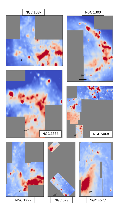
After KCWI datacubes had been aligned and flux calibrated to match the MUSE mosaics, the KCWI datacubes were co-added to create KCWI galaxy mosaics. The image co-addition was performed with Montage. The mAddCube call to Montage initiates the co-addition. The co-addition is performed by stacking the aligned images, according to the an output WCS determined by Montage, and then taking the average value between any overlapping pixels. Pseudo -band images for the final mosaics of each galaxy are shown in Figure 1.
3.6 Absolute calibration of KCWI Compared to MUSE
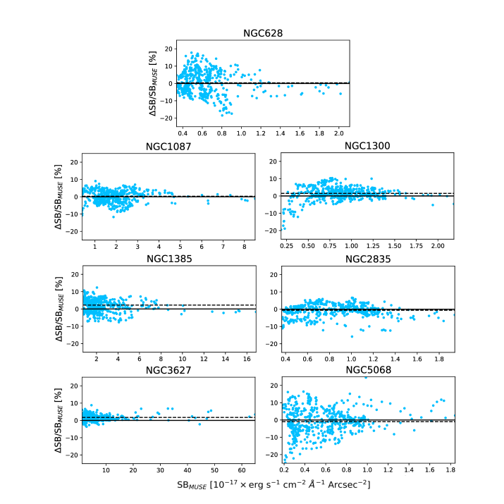
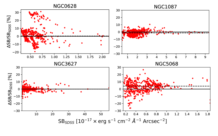
We assesed the absolute calibration of the co-added KCWI mosaics by comparing the SB’s between the KCWI and MUSE mosaics. Comparisons of the MUSE mosaics with SDSS imaging in the -band described in Emsellem et al. (2022) showed that the MUSE absolute flux calibration is consistent with SDSS calibration within the instrument uncertainty of mag (Padmanabhan et al., 2008). We calculated the SB inside apertures, randomly placed in the KCWI coverage. The SB offsets between the KCWI and MUSE mosaics are shown in Figure 2. The resulting offsets, summarized in Table 2, reveal acceptable agreement between the MUSE and KCWI absolute calibration. The average percent SB offset with respect to the SDSS imaging, , is between % and % with a median value across all galaxies of % 4%.
3.7 Absolute calibration of KCWI Compared to SDSS
We have shown agreement between KCWI and MUSE, but this comparison is only an assessment of the flux calibration in the overlapping wavelength range of KCWI and MUSE. To assess the absolute flux calibration across a wider wavelength range, we compared synthetic g-band images of the KCWI mosaics to Sloan Digital Sky Survey (SDSS, Abazajian et al., 2003) images of the same galaxies. Only four galaxies with KCWI mosaics have SDSS imaging: NGC 628, NGC 1087, NGC 3627 and NGC 5068. We constructed synthetic g-band images of these galaxies by convolving the spectrum in each pixel, , with the -band transmission curve, , according to the following equation:
| (1) |
The SDSS imaging is presented in units of nanomaggies or 3.631 Jy. To compare with the KCWI data, with native units of flux density, , we converted to flux density with the following expression (Tokunaga & Vacca, 2005),
| (2) |
where is the pivot wavelength of the band-pass. The pivot wavelength for the g-band filter is Å. The surface brightness for both KCWI and SDSS are measured inside radius apertures. The mean and 1 scatter of the measured surface brightness are shown in Figure 3. We found overall agreement of the absolute calibration between KCWI and SDSS for the four galaxies. Summarized in Table 2, the median offset across the sample galaxies, range between 1.0% and 3.0% and exhibits scatter between 3% and 10%. The largest scatter appears to be limited to a single field of NGC 628 that only contains signal from a single, isolated region, and will have negligible impact on the remaining analysis. The median offset across all galaxies is % which suggests that the KCWI calibration is in good agreement with SDSS.
| Name | SB)aaThe median fractional surface brightness offset between KCWI and MUSE in %. | SB)bbThe standard deviation of the fractional surface brightness offset between KCWI and MUSE in %. | SBg)ccThe median -band surface brightness offset between KCWI and SDSS. | SBg)ddThe standard deviation of -band surface brightness offset between KCWI and SDSS. | ||
|---|---|---|---|---|---|---|
| [%] | [%] | [%] | [%] | |||
| NGC 628 | 0\@alignment@align.3 | 6.0 | 0\@alignment@align.3 | 10.0 | ||
| NGC 1087 | 0\@alignment@align.5 | 3.6 | -1\@alignment@align.0 | 3.4 | ||
| NGC 1300 | 1\@alignment@align.5 | 4.0 | -\@alignment@align | - | ||
| NGC 1385 | -0\@alignment@align.6 | 4.3 | -\@alignment@align | - | ||
| NGC 2835 | -0\@alignment@align.4 | 3.6 | -\@alignment@align | - | ||
| NGC 3627 | 1\@alignment@align.7 | 1.6 | -0\@alignment@align.05 | 2.6 | ||
| NGC 5068 | 0\@alignment@align.3 | 6.7 | 2\@alignment@align.9 | 8.4 | ||
4 H II Region Catalog
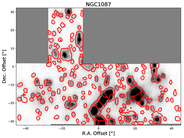
In order to assess the emission line properties of H ii regions, we determine the H ii region location and boundaries using H maps constructed from the KCWI spectral datacubes and the image segmentation software HIIphot (Thilker et al., 2000). Although H ii region masks have previously been constructed from the MUSE H maps for these galaxies (Kreckel et al., 2019; Santoro et al., 2022; Groves et al., 2023; Congiu et al., 2023), the MUSE angular resolution is higher than that of KCWI. Because of this, the H ii region boundaries derived from MUSE may not fully encapsulate the spatial extent of the H ii regions observed using KCWI. Furthermore, simply convolving or reprojecting the MUSE H ii masks to the KCWI resolution or grid would introduce uncertainty on the boundaries for tightly spaced H ii regions. We therefore perform H ii region identification directly on the KCWI data.
4.1 Construction of H Maps
H is the brightest H I recombination line observed by KCWI, and maps of this emission for the galaxies will be used to define our H ii regions. The continuum near and underlying H emission must be removed in order to accurately map its emission. To remove the continuum we used LZIFU, an emission line fitting code designed specifically for use with IFUs (Ho et al., 2016). LZIFU implements and streamlines the penalized pixel-fitting software (PPXF, Cappellari & Emsellem, 2004; Cappellari, 2017) for using PPXF on IFU emission line maps. To fit the continuum of the input spectrum LZIFU matches a series of input single-metallicity, [Z/H] , stellar population models (Vazdekis et al., 2010, MILES) that have been redshifted, and convolved to match the input spectrum PSF. LZIFU fits Gaussian models at the location of emission lines. In the output H map, pixels with weak or no H can contain ‘NaN’ values which can be problematic for HIIphot. To avoid these artifacts, we subtract the stellar continuum from each pixel’s spectrum and construct the final H maps by integrating the continuum-subtracted spectra between 4856–4876 Å. The final maps are suitable for H ii region identification using HIIphot.
4.2 H II Region Identification
HIIphot was designed to identify H ii regions and complexes (unresolved or blended H ii regions) while also minimizing the inclusion of surrounding diffuse ionized gas (or DIG). HIIphot works by first defining “seeds” at the location of peak emission in H (or H), then iteratively grows each “seed” and terminates only when the gradient of the H (or H) surface brightness distribution matches a termination value, in mandatory units of emission measure (EM), set by the user. The gradient of the surface brightness distribution is more robust method of stopping uncontrolled growth at lower S/N compared to using only the average local background level. For each galaxy we apply the the same termination gradient, 5 EM pc-1 or 2.43 , as the recent PHANGS-MUSE work by Santoro et al. (2022).
HIIphot uses the PSF to convolve the input H map to different spatial scales to identify seeds. Using a constant PSF for all galaxies can potentially miss valid regions or generate non-physical regions. The PSF of the input H emission map is required by HIIphot. For each galaxy mosaic, we used the average PSF from the its KCWI pointings (see Table 7 in Appendix A) as the input for HIIphot. The resulting 2D mask returned by HIIphot contains H ii regions with smooth and reasonable boundaries, judged by the distinction between clearly separated HII regions, the minimization of spurious small and pixelated regions or runaway growth. In total, HIIphot identifies 688 H ii regions or complexes across all of the KCWI mosaics. This number is smaller than the 2169 potential H ii regions identified for the Nebular catalog (Kreckel et al., 2019; Santoro et al., 2022; Groves et al., 2023), and 2124 potential H ii regions from Congiu et al. (2023), inside the same KCWI footprints. This is largely due to the differences in angular resolution between KCWI and MUSE, and the three-fold decrease in strength of H emission relative to H. In Figure 20 of Appendix C we show histograms of the H luminosity and radii for KCWI and Nebular catalog regions as well a comparisons of the spatial masks in Figures 21–27 of Appendix C. Additionally, we also present in Table 9 of Appendix C the number of regions detected per galaxy.
4.3 Generation of Integrated H II Region Spectra
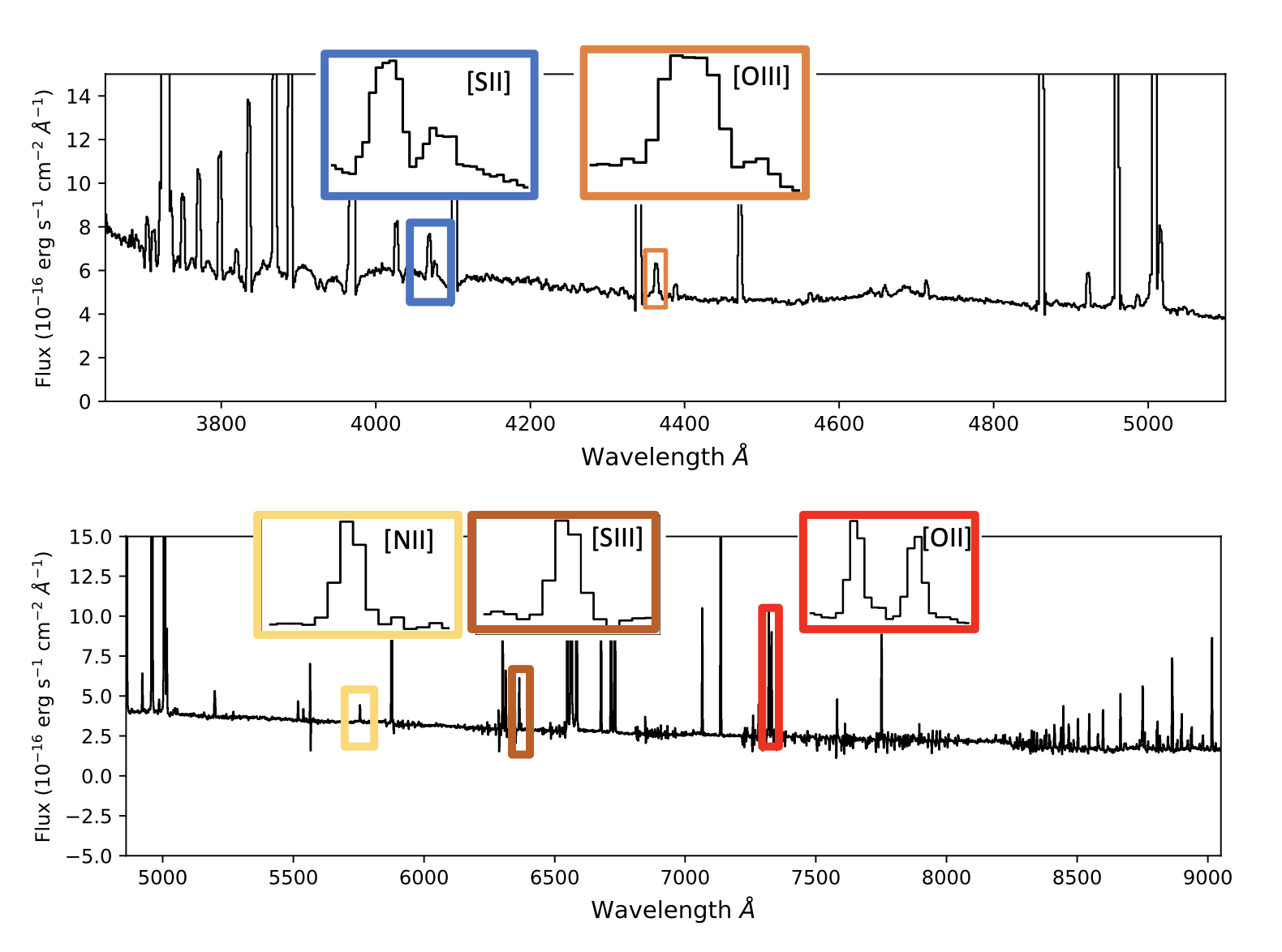
The KCWI H ii region masks, produced by HIIphot, are used to isolate and sum the spectra in pixels belonging to each H ii region, resulting in an integrated H ii region spectrum. To produce a matching MUSE H ii region mask we transformed the H ii regions coordinates/boundaries from the KCWI pixel grid onto the MUSE pixel grid. These are then used to construct MUSE integrated spectra for each H ii region. The KCWI and MUSE H ii region spectra for a single H ii region, with the full set of auroral lines highlighted, is shown in Figure 5.
We also produce integrated variance spectra for each H ii region. The variance spectra for both KCWI and MUSE H ii regions are constructed by propagating the pipeline-produced variance datacubes for pixels contained within each H ii region boundary. In the case of MUSE, the datacubes have undergone an additional convolution process in order to generate mosaics with uniform PSF which introduces a correlation between neighboring pixels (Emsellem et al., 2022). Because of the additional convolution, we generated the MUSE variance spectra, assuming fully correlated conditions, by adding the pixel variance spectra linearly (Taylor, 1997).
We verify this choice by comparing the median standard deviation of the propagated MUSE variance spectra, , to the median standard deviation of the H ii region spectrum, , in the emission line free wavelength range Å. We measured an average ratio between the propagated and measured error of , implying that we are appropriately propagating the error. We also perform a similar comparison for KCWI, and find agreement, , between the measured and propagated error using uncorrelated pixel error propagation. To generate the appropriate variance we propagated the error using uncorrelated, for KCWI, and fully correlated error, for MUSE, propagation methods.
4.4 H II Region Stellar and Emission Line Fitting
We modeled the stellar continuum and emission lines of the integrated H ii region spectra using the general PPXF toolkit. Although the LZIFU implementation of PPXF allowed for the streamlined, full datacube, fitting of the KCWI H emission line map, the general PPXF toolkit offers more flexibility in the input fitting parameters. For example, we can input a wavelength dependent LSF function as well as fix the kinematics between emission lines of doublets and lines with similar levels of ionization. We followed Emsellem et al. (2022) and fit the emission lines simultaneously with the stellar continuum. This particular fitting recipe was chosen to mirror the philosophy of the Mapping Nearby Galaxies at APO Data Analysis Pipeline (MaNGA DAP, Law et al., 2016; Emsellem et al., 2022) and is suggested to mitigate the biases on emission line fluxes introduced from the masking of stellar absorption features around affected lines (Sarzi et al., 2006; Oh et al., 2011; Belfiore et al., 2019). PPXF robustly fits the stellar continuum by matching a set of templates to the observed H ii region spectrum. The templates originate from the E-MILES library of simple stellar population (SSP) models (Vazdekis et al., 2016). The SSP ages were between Gyr. Each age bin contained SSPs with the following metallicities, . Typically, PPXF convolves the SSP templates with a Gaussian model accounting for the spectral resolution of the input spectrum and the stellar velocity dispersion. However, because the KCWI line profile deviates significantly from a Gaussian (see Appendix B) we convolved the PPXF templates with a 4-moment Gauss-Hermite function while fitting KCWI emission lines. We constrained the fits of and in the Gauss-Hermite functions to values listed in Appendix B. We performed the PPXF fitting of the KCWI H ii region spectra independently from the MUSE H ii region spectra. The fractional difference between the H ii region H flux for KCWI and MUSE is .
We obtained errors on the emission line fluxes from the output of PPXF. The output errors are considered reliable if the PPXF derived reduced . Together the resulting fits for both the KCWI and MUSE have an average reduced , indicative the input variance spectra are under-estimated. We obtained a better estimate of the errors by re-scaling the returned errors, for each fit to KCWI and MUSE spectra, by a factor of (Cappellari & Emsellem, 2004; Cappellari, 2017; Emsellem et al., 2022).
4.5 Dust Correction
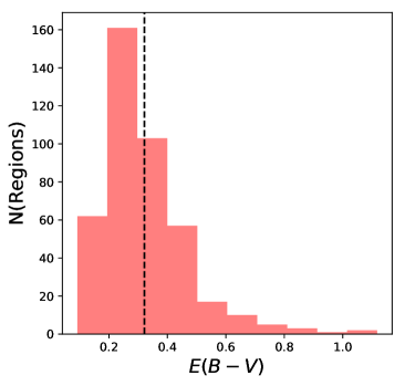
We derive the V-band extinction () for each H ii region using the Balmer decrement. To evaluate this decrement while also taking into account the errors on the measured H and H emission, we construct a distribution of the MUSE H/H ratios by sampling the error for each line. Next, using PyNeb, we calculate the extinction by comparing the average of the H/H distribution to the theoretical value assuming the Case B recombination conditions 103 cm-3 and K (Storey & Hummer, 1995). We explore how changing the assumed could affect the derived by sampling a range of temperatures between 5000 K and 1.5 K and find that the standard deviation of for a fixed Balmer decrement is mag. We apply the wavelength dependent extinction correction assuming a O’Donnell (1994) extinction curve. We present a histogram of the derived E(-) in Figure 6. The average E(-) for the regions is mag and corresponds to an mag. We find a negligible difference when using KCWI H in place of the MUSE H flux. We add that a recent investigation shows that correcting, or not correcting, the Balmer lines for DIG contamination can impact the measured E(-) (Congiu et al., 2023). For the range of E(-) observed, a DIG-corrected E(-) may return values of 0.05–0.1 mag lower than presented here. We discuss the effects that under/over-estimated extinction may have on the measured electron temperature in Section 7.1.1.
4.6 Diffuse Ionized Gas
Emission from Balmer transitions, [S II], [N II], and other lines originating from DIG surrounding the H ii regions can contaminate the H ii region emission line fluxes of the same transitions. Measuring the DIG contribution to H ii region line flux is only beginning to being explored by IFU studies (see Belfiore et al., 2022; Congiu et al., 2023). In order to removes regions with large degree of DIG contamination we calculate the contrast between H ii/DIG emission following the scheme outlined in Kreckel et al. (2022). First, we mask each H ii region in the MUSE emission line maps for: H, H, [S II], [N II] and [O I]. For each emission line, we place a aperture around each H ii region and measure the median DIG flux in pixels with and H surface brightness (see Belfiore et al., 2022). Finally, we calculate the “integrated” DIG emission by multiplying the median DIG flux by the H ii region size. For each DIG emission line, we calculate the percent contrast between the measured H ii region flux and DIG flux. If the contrast between the H ii region flux and DIG flux of any low-ionization emission line is %, we exclude it from the sample.
4.7 Quality Assessment and Classification of Regions
The regions identified by HIIphot are potentially a mix of H ii regions, planetary nebulae, and supernova remnants. Some also have low S/N. We perform a set of cuts to reject non-H ii regions and/or low S/N spectra from the catalog of H ii regions.
-
•
We exclude any H ii region whose centroid coordinates are within 2″ from the edge of the mosaic. This step removes 86 H ii regions
-
•
We require the strong lines used for temperature determinations: H, H, [O III] [O II], [N II], [S III] and [S II] to be detected above a threshold of S/N 5. This step cuts 72 H ii regions from the sample.
-
•
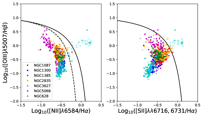
Using the lines of H, H, [O III] and [N II] we construct a Baldwin-Phillips-Terlevich (BPT, Baldwin et al., 1981) diagram. We require H ii regions to be consistent with photoionization by massive stars. Therefore, we require them to fall below the empirical [O III]/H vs. [N II]/H (Kauffmann et al., 2003) and [O III]/H vs. [S II]/H (Kewley et al., 2001) lines. The BPT diagram showing the location of each H ii region is shown in Figure 7. Out of the sample, 11 H ii regions are above the empirical and theoretical line cut-offs and are removed.
-
•
We exclude H ii regions that fail our DIG contrast check in Section 4.6. This step removes 98 H ii regions.
The constraints together remove 267 out of the 688 detected H ii regions leaving 421 H ii regions remaining for use in our analysis. For the final sample, comparison of line ratios in Figure 7 to model classifications in Figure 3 of Congiu et al. (2023) suggest that final sample is consistent with their H ii region classification.
5 Measurement of Auroral Line Emission
In order to robustly measure the flux and uncertainty for the faint, temperature sensitive auroral lines from [N II], [O II], [S II], [O III], and [S III] we implement a specific auroral line fitting scheme in place of PPXF. This is necessary because any under/over subtraction of the continuum at the location of the faint auroral lines can bias the measured auroral line flux.
The framework of the auroral line fit is as follows. We first subtract the stellar continuum spectrum fitted by PPXF. This results in an H ii region spectrum that contains only emission lines and residuals from the continuum subtraction. Next, we measure the standard deviation of the residuals, , in a region near the auroral line but also free of emission. We then perform a large number of fits to the auroral line with random noise added to each wavelength bin, drawn from a normal distribution with standard deviation . In each trial, we fit a single Gaussian (or double depending on the auroral line) plus constant continuum level to the the spectrum. The constant term is needed to correct for any remaining continuum present in the continuum-subtracted spectrum. After completing the trials, we calculate the average integrated line flux, , and the standard deviation of the measured fluxes, . If S/N we consider the auroral line detected. In Figure 29 of Appendix D we show the model fits and residuals for a region in NGC 5068.
Although this general process is performed for all the auroral lines, the auroral line from [OIII] is subject to additional constraints because emission from the [O III] can be blended with [Fe II]. This has been observed in both stacked galaxy and individual H ii region spectra (Curti et al., 2017; Berg et al., 2020; Arellano-Córdova & Rodríguez, 2020). The strength of the [Fe II] has been observed to increase with the metallicity of the gas (Curti et al., 2017), although continuum pumping fluorescence contributes strongly to its emissivity (Rodríguez, 1999). [Fe II] and [Fe II] arise from the same atomic upper level and their relative intensities are independent of the physical conditions of the gas and depend solely on the atomic transition probabilities. Since (Mendoza et al., 2023), if [Fe II] is detected, [Fe II] should be present too.
To remove blending of the [O III] line by [Fe II], we use the fixed ratio, , to estimate the degree of contamination by measuring the strength of the brighter [Fe II] emission. We first fit the [Fe II] line using a single Gaussian plus a constant continuum level model. The initial guesses for the line center and width are taken from the parameters of H returned by the PPXF fits. In the case that the [Fe II] is not detected above a S/N threshold of 3, we instead use the 3 upper limit. We next fit [O III] using a single Gaussian plus constant offset model. The initial guesses for the kinematics of [O III] are taken from the PPXF fit of [O III]. After adding random noise, we generate a model for the [Fe II]4360 using the best fit parameters and errors derived from the fit to [Fe II], using the fixed ratio. After generating the [Fe II]4360 model, we subtract it from the trial spectrum and proceed to then fit for the emission line flux originating from [O III]. We detect emission from [Fe II] in 30 H ii regions, two of these are in regions with measurable [O III]. From these, we determined that the 3 upper-limit on the [Fe II] flux is 3.5 which is of the average [O III] flux. We show in Figure 30 Appendix D an example [O III] fit which has had significant [Fe II] contribution removed.
6 H II Region Nebular, Environmental, and Stellar Properties
We assess the ionized gas physical conditions—, , and ionization parameter —of each H ii region using a subset of the dust-corrected emission line fluxes. We also measure a number of characteristics of the H ii region’s environment and local stellar population, as described below.
6.1 Electron Density
Using PyNeb we calculate the electron density for each H ii region using the [S II] doublet. Based on our constraints discussed in Section 4.7, each H ii region is guaranteed to have measured emission from this doublet at S/N . The [O II] doublet is also commonly used to estimate . The atomic levels responsible for [S II] and [O II] both have critical densities, when collisional and radiative de-excitation are occurring at equal rates, that are of order cm-3. The critical densities, as well as other references for the atomic data used, are listed in Table 3. Both the [S II] and [O II] doublets are sensitive to densities . However, in the KCWI measurements, the [O II] doublet is unresolved, and therefore we do not use it to measure . With the exception of a handful of regions, the measured electron densities are in the low-density limit, .
| Ion | Transition Probabilities | Collision Strengths | |
|---|---|---|---|
| ( cm-3) | |||
| O II | Zeippen (1982) | Kisielius et al. (2009) | 2aaAverage critical density for [O II] . |
| O III | Froese Fischer & Tachiev (2004) | Storey et al. (2014) | 691 |
| N II | Froese Fischer & Tachiev (2004) | Tayal (2011) | 88 |
| S II | Rynkun et al. (2019) | Tayal & Zatsarinny (2010) | 3bbAverage critical density for [S II] . |
| S III | Froese Fischer et al. (2006) | Tayal & Gupta (1999) | 543ccAverage critical density for [S III] . |
6.2 H II Region Electron Temperatures
The auroral lines allow the determination of the electron temperatures for the O+, O2+, N+, S+ and S2+ ions, or , , , , and , respectively. The temperatures are calculated via PyNeb using the collision strengths and transition probabilities, listed in Table 3, as well the measured upper-limits of the electron density, , to convert an auroral-to-nebular ratio to temperature. The critical densities of the requisite lines, see Table 3, used to estimate , , and are high enough such that the auroral-to-nebular lines ratios are insensitive to choice of . The density sensitivity in the lines used for and begins at smaller densities and is further discussed in Section 7.2. The uncertainty for each temperature measurement is the standard deviation of the distribution of temperatures constructed by Monte Carlo sampling of the error for each auroral and nebular line included in the temperature determination. We summarize the number of detections and median temperature for each ion in Table 4.
| Te,Ion | MedianaaThe 50th the 16th – 84th percentile of the measured temperatures. | bbNumber of H ii regions with temperature measured from the particular ion. |
|---|---|---|
| [104 K] | ||
| 0.95 | 156 | |
| 0.81 | 245 | |
| 0.94 | 305 | |
| 0.89 | 143 | |
| 1.20 | 26 |
6.3 H II Region Ionization Parameters
The ionization parameter is an indicator of the strength of the ionizing radiation field. The Strömgren sphere descriptions of H ii regions define the ionization parameter as , where is the emission rate of photons capable of ionizing hydrogen (i.e., with energy eV), is the radius of the ionized region, and are the hydrogen density and speed of light. However, calculating the ionization parameter using this definition is difficult (Kreckel et al., 2019, 2022) as resolved studies show that H ii regions exhibit a range of non-spherical morphologies and non-uniform densities (Wood & Churchwell, 1989).
Instead, we trace the ionization parameter using the [S III]/[S II] and [O III]/[O II] emission line ratios. Photoionization modeling has shown that both the [S III]/[S II] and [O III]/[O II] correlate with the ionization parameter, (Dors et al., 2011). Although it has a positive correlation with the ionization parameter, the [O III]/[O II] also has a secondary dependence on metallicity, increasing with decreasing metallicity. [S III]/[S II] is not as sensitive to metallicity, making the ratio a more reliable tracer of the ionization parameter (Kewley & Dopita, 2002). While [S III] is not observed with MUSE, we measure the [S III] and assume the fixed theoretical line ratio of [S III] (Froese Fischer et al., 2006) in all calculations.
6.4 ALMA-CO: Intensity, Peak Temperature, and Velocity Dispersion
Using the ALMA 12m+7m+TP datacubes, we calculate moment 0, and 2 (integrated intensity and velocity dispersion) for molecular gas near each H ii region. Because molecular and ionized gas are not entirely co-spatial at our resolution, it is necessary to make a selection to capture gas near the H ii region. One possibility is to match H ii regions to molecular clouds via a nearest-neighbor algorithm (Grasha et al., 2019; Zhang et al., 2021; Zakardjian et al., 2023) We instead choose to integrate the ALMA spectrum contained in the H ii region boundaries in order to measure the properties of the molecular gas closest in projection to the the ionized gas (i.e. in front, behind, or blended due to the resolution of KCWI) and likely affected by the radiative feedback. To measure the CO spectra, we reproject the H ii region masks onto the grid of the ALMA datacubes and integrate the ALMA spectra for pixels located inside the footprint of each H ii region.
From the ALMA spectrum, we then calculate the integrated intensity, , peak temperature, and the velocity dispersion, . In order to accurately measure these CO moments in the presence of noise, we construct a signal mask following the basic approach from Leroy et al. (2021b). To do this, we locate the velocity channel which contains the peak emission and construct an integration window around this channel by including velocity channels with signal above the noise.
As a check on our analysis of molecular gas, we compare the calculated velocity dispersions to those from a sample of nearest-neighbor matched H ii regions-GMC’s constructed by Zakardjian et al. (2023). We find that our span a similar range, up to Log10([km s-1])=1.5, with an average and standard deviations of Log[km s-1])=0.88 0.25; in line with the average from Zakardjian et al. (2023) which suggests that this method of extracting and measuring the CO properties is reasonable.
6.5 H ii Region Compact Clusters and Associations
In order to test for correlations between the young stellar populations that power H ii regions and their electron temperatures, we compile the stellar mass and age of compact clusters and multi-scale stellar associations within our KCWI H ii regions using results from HST observations.
We match the HST clusters to individual H ii regions by simply selecting all the clusters whose on-sky coordinates fall inside any H ii region’s spatial footprint. For the associations, we match the NUV selected, 32 pc scale, stellar associations to the individual H ii regions in the same manner as Scheuermann et al. (2023). The associations catalog comes with spatial masks identifying the footprint of all the detected associations. Because the association masks have a finer pixel scale than the KCWI H ii region masks, we reproject the KCWI mask onto the association mask pixel grid. We find for cluster matches that only 99 or 23.5% of our H ii regions are matched to a single cluster. 274 or 65% of our H ii regions have zero matches. For association matches, only 149 or 35.4% of our H ii regions are matched to a single association 117 or 27.8% of our H ii regions have zero matches.
For the remaining regions with more than one clusters or association match, because we expect that the youngest and most massive clusters or associations contribute most to the overall ionization of the H ii region, we assign to each H ii region the age (mass) of the youngest (most massive) available cluster/association.
7 Results
We present electron temperatures derived using the auroral-to-nebular line ratios from [O II], [N II], [S II], [S III], and [O III]. We construct – diagrams to compare any multi-ionization zone relationships to recently measured and/or modeled trends. We then compare the temperatures to properties of the ionized gas such as electron density, , and ionization parameter, . We also relate the temperatures to properties of the molecular gas and stellar populations.
7.1 Temperature-Temperature Relations
7.1.1 Low-Ionization Zone
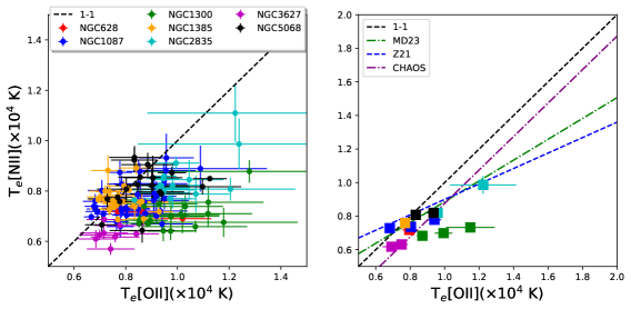
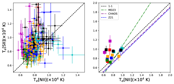
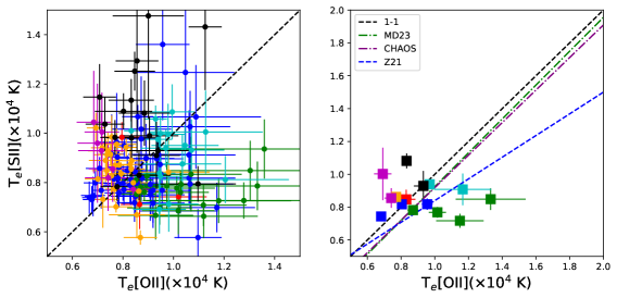
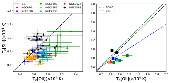
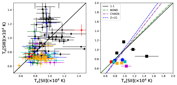
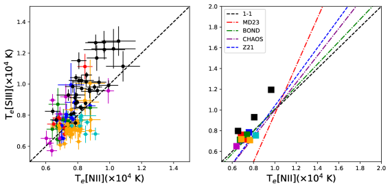
We show – relations for our sample H ii regions in Figures 8, 9 and 10. The left panel displays the individual H ii region measurements. To better see – relationships in individual galaxies we show in the right panel the – relations for temperatures binned in steps of 2000 K in the x-axis, with minimum 2 H ii regions per bin, for each galaxy. Alongside the binned data we show recent – relations from Berg et al. (2020, hereafter CHAOS), Zurita et al. (2021, hereafter Z21), Garnett (1992, hereafter G92), Vale Asari et al. (2016, hereafter BOND), and Méndez-Delgado et al. (2023b, hereafter MD23).
The low-ionization zone – relations are shown in Figure 8. The top figure shows the – comparison. We observe that gives higher values than by 1000 K on average. The magnitude of this offset is largest when K. The inequality is also reflected in the relations from Z21, CHAOS, and MD23. With the exception of the CHAOS trend, the slope of the relations also indicate a steeper rise in than . Although the data lie below the 1–1 line, they also do not clearly prefer either CHAOS, MD23, and Z21 relations.
The comparison between – is shown in the middle panel of Figure 8. We observe that there is an offset in between – in favor of hotter . Similar to –, the scatter in the temperatures is larger in rather than . A majority of the binned data points congregate above the literature relations. Only a few exceptions agree with the 1–1 line.
We show the temperatures for 129 regions with both - in the bottom-left panel. We observe large scatter for both and . Again, the binned data do not strongly prefer any of the selected relations.
We observe in the – relations that and are systematically hotter than . Based on photoionization models (e.g., Campbell et al., 1986; Garnett, 1992), the low-ionization zone temperatures are expected to be equal. There are systematic effects that could increase and temperatures such that . The wide wavelength range between [O II] and [O II] as well as [S II] and [S II], make these ratios sensitive to the applied reddening correction. An overestimate in the extinction would lead to an underestimate of and underestimate of . At the same time this would leave relatively unchanged due to the closeness in wavelength of the requisite lines. We see that both and are greater than which is not compatible with the effects of overestimated extinction correction. Despite the above, our temperatures hierarchy could potentially be produced by under-estimated extinction as this would lead to over-estimates of and while again leaving unchanged. We tested two different extinction prescriptions (O’Donnell, 1994; Fitzpatrick, 1999) and found no change in our results. Due to the possible DIG contribution to the measured extinction, it is more likely that we could be overestimating the extinction than underestimating it. Telluric contamination to the line emission at [O II] could be an additional systematic error, but is unlikely to be significant in our data because the [O II]/ ratio measured for our sample is , in agreement with values predicted by the transition probabilities and the collisional strengths (Zeippen, 1982; Kisielius et al., 2009) and observed in nearby H ii regions (Seaton & Osterbrock, 1957; Kaler et al., 1976; Yates et al., 2020; Méndez-Delgado et al., 2022). The [S II] doublet may contain contamination due to O II recombination emission near the location of [S II] (Méndez-Delgado et al., 2023b) that could bias upwards by K for K. The KCWI spectral resolution is too low to separate out any contamination in the measurements of [S II]. Lastly, and have a higher sensitivity to electron density inhomogeneities than (Rubin, 1989; Osterbrock & Ferland, 2006; Méndez-Delgado et al., 2023b). [O II] and [S II] start to be dependent on density around cm-3 while [N II] is independent of density up to cm-3. We explore this dependence further in Section 7.2.
7.1.2 Intermediate Ionization Zone
The – relations between the low and intermediate-ionization zone temperatures are shown in Figure 9. Given the lower ionization potentials of O+, N+, and S+ with respect to S++, it is possible to have differences in the temperature in the different ionization zones (Garnett, 1992). We compare our observed – relations to predictions from photoionization models for giant H ii regions produced by the Bayesian Oxygen and Nitrogen abundance project BOND and found in the Mexican Million Models database (Morisset, 2009). When available, we also compare the observations to relations from CHAOS, MD23, and Z21.
The top panel of Figure 9 shows the temperature comparisons between and . The (BOND) models predict that the temperature should be greater than by a small constant offset across the full temperature range. However, our data suggest rises faster than . Our binned data favor the empirical trend line from Z21. However, there is a grouping of points from NGC 5068 that show contrasting behavior in both the individual and binned data comparisons.
The and comparison, comprised of 108 H ii regions, is shown in the middle panel of Figure 9. We observe in the middle-left panel scatter K with no clear trend for higher or lower temperatures on either axis. The binned data do not reveal a preference for any trend.
The bottom panel of Figure 9 shows the and comparison. and exhibit the smallest scatter, K, of the – relations presented here. In the left panel, we see that with increasing , the trend of the individual points slightly favor hotter . For the and comparison there are available empirical relations from CHAOS, Z21, and MD23 which we overlay in addition to the BOND models. We observe a large fraction of the binned data that lie near the CHAOS model, and Z21 relations at low . Regions with hotter and would be needed to to further differentiate between the models and empirical trends.
7.1.3 High Ionization Zone
We show – relations between [O III] temperatures (which trace the high ionization zone) and those from the low/intermediate ionization zones in Figure 10. Additionally, we overlay – relations from CHAOS, Z21, and G92. Although we observe some H ii regions with – relations that agree with literature relations, we also observe numerous H ii regions with much higher values of than what is predicted by models with the given low and intermediate ionization zone temperatures.
The large excess in for regions with cooler low and intermediate ionization zone temperatures is unexpected. At the Solar metallicities of our sample, the relative flux [O III] is expected to be H (Berg et al., 2015). The small number of [O III] detections reflects this. Because we do not expect to detect the line in most H ii regions, the ones we do detect may be unusual cases or statistical outliers, especially given that the average S/N of the [O III] detections is 4. Despite this, there has been evidence (Peimbert et al., 1991; Binette et al., 2012) that shock excitation can preferentially enhance the high ionization zone temperature. This scenario is explored in Section 7.2.5.
7.2 Temperature Differences Compared to H II Region, Stellar Population, and Molecular Gas Properties.
Studies have shown that H ii region temperatures for different ionization zones can be differently impacted by the ionization state of the gas (Berg et al., 2020; Arellano-Córdova & Rodríguez, 2020; Yates et al., 2020) and by temperature/density fluctuations (Méndez-Delgado et al., 2023a, b). However, the physical processes that drive these differences in temperature remain poorly constrained and uncertain (Garnett et al., 1991; Nicholls et al., 2020). The KCWI+MUSE H ii region observations allow us to investigate potential sources driving temperature differences, (,)=, between the low, intermediate, and high-ionization zone temperatures. We compare temperature differences with H ii region properties derived from emission line diagnostics; with the properties of the surrounding molecular gas measured from ALMA (Leroy et al., 2021b); and with stellar population masses/ages from SED fitting to HST photometry (Lee et al., 2022; Thilker et al., 2022; Larson et al., 2023).
We summarize the comparisons to ionized gas properties in Table 5 and the molecular gas/stellar population properties in Table 6. To gauge the significance and degree of correlation between each comparison we calculate the Spearman Rank Correlation Coefficient, , and associated p-value, . A correlation is judged to be significant if it exhibits . The strength of the correlation is separated into the following regimes: corresponds to a strong correlation, corresponds to a moderate correlation and identifies a weak or no correlation.
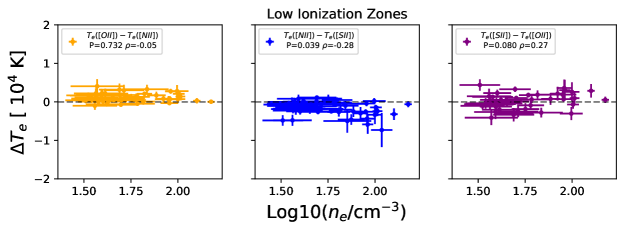
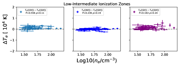
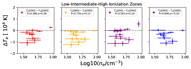
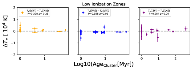
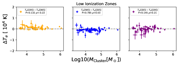
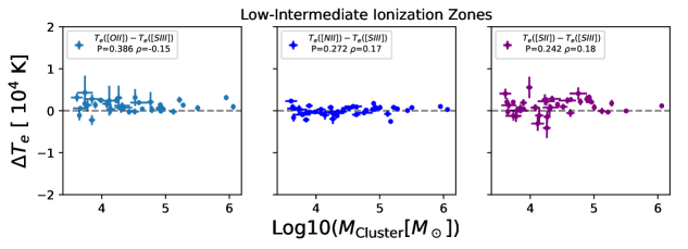
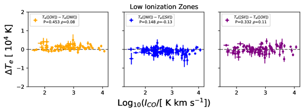
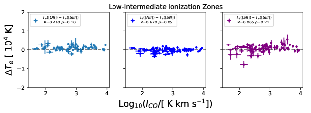
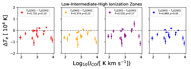
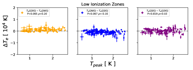
We do not report any significant correlations between with any of the following properties: , integrated CO intensity, CO peak temperature, cluster mass, cluster age, and association age. Figures showing the comparisons to these parameters are shown in Appendix E. However, we do measure correlations with ionization parameter, association mass, and molecular gas velocity dispersion. We discuss these correlations in the following subsections.
| [S III]/[S II] | [O III]/[O II] | |||
|---|---|---|---|---|
| (, p) | (, p) | (, p) | ||
| (, ) | (0\@alignment@align.00, 0 | (0.02, 0.79) | (-0\@alignment@align.05, 0 | |
| (, ) | (-0\@alignment@align.34, ) | (-0.03, 0.66) | (-0\@alignment@align.28, 0 | |
| (, ) | (0\@alignment@align.34, ) | (0.07, 0.40) | (0\@alignment@align.27, 0 | |
| (, ) | (0\@alignment@align.06, 0 | (0.02, 0.82) | (0\@alignment@align.11, 0 | |
| (, ) | (0\@alignment@align.26, 0 | (0.02, 0.81) | (0\@alignment@align.19, 0 | |
| (, ) | (0\@alignment@align.54, ) | (0.03, 0.70) | (0\@alignment@align.24, 0 | |
| (, ) | (0\@alignment@align.62, ) | (0.85, ) | (0\@alignment@align.38, 0 | |
| (, ) | (0\@alignment@align.72, ) | (0.82, ) | (0\@alignment@align.13, 0 | |
| (, ) | (0\@alignment@align.78, ) | (0.78, ) | (0\@alignment@align.15, 0 | |
| (, ) | (0\@alignment@align.59, 0 | (0.80, ) | (0\@alignment@align.00, 1 | |
| AgeCluster | MCluster | AgeAssoc | MAssoc | |||||||
|---|---|---|---|---|---|---|---|---|---|---|
| (, p) | (, p) | (, p) | (, p) | (, p) | (, p) | (, p) | ||||
| (, ) | (-0\@alignment@align.25, 0 | (-0.22, 0.13) | (0\@alignment@align.0, 0 | (-0.11, 0.35) | (0\@alignment@align.08, 0 | (0.20, 0.07) | (-0\@alignment@align.16, 0 | |||
| (, ) | (-0\@alignment@align.01, 0 | (0.03, 0.79) | (0\@alignment@align.04, 0 | (0.12, 0.20) | (-0\@alignment@align.13, 0 | (-0.16, 0.67) | (0\@alignment@align.01, 0 | |||
| (, ) | (0\@alignment@align.00, 0 | (0.21, 0.15) | (-0\@alignment@align.12, 0 | (-0.06, 0.61) | (0\@alignment@align.11, 0 | (0.03, 0.82) | (0\@alignment@align.11, 0 | |||
| (, ) | (-0\@alignment@align.04, 0 | (-0.15, 0.39) | (-0\@alignment@align.02, 0 | (0.11, 0.43) | (0\@alignment@align.10, 0 | (0.15, 0.28) | (0\@alignment@align.14, 0 | |||
| (, ) | (-0\@alignment@align.08, 0 | (0.17, 0.28) | (-0\@alignment@align.23, 0 | (0.37, 0.001) | (0\@alignment@align.05, 0 | (-0.21, 0.62) | (0\@alignment@align.39,) | |||
| (, ) | (-0\@alignment@align.32, 0 | (0.18, 0.24) | (-0\@alignment@align.21, 0 | (0.13, 0.25) | (0\@alignment@align.21, 0 | (0.08, 0.52) | (0\@alignment@align.24, 0 | |||
| (, ) | (0\@alignment@align.19, 0 | (-0.42, 0.09) | (0\@alignment@align.65, 0 | (-0.51, 0.02) | (0\@alignment@align.10, 0 | (0.37, 0.16) | (-0\@alignment@align.51, 0 | |||
| (, ) | (0\@alignment@align.30, 0 | (-0.40, 0.12) | (0\@alignment@align.45, 0 | (-0.33, 0.12) | (0\@alignment@align.23, 0 | (0.46, 0.05) | (-0\@alignment@align.45, 0 | |||
| (, ) | (0\@alignment@align.30, 0 | (-0.37, 0.15) | (0\@alignment@align.32, 0 | (-0.47, 0.03) | (0\@alignment@align.17, 0 | (0.42, 0.90) | (-0\@alignment@align.44, 0 | |||
| (, ) | (0\@alignment@align.48, 0 | (-0.39, 0.15) | (0\@alignment@align.42, 0 | (-0.42, 0.63) | (0\@alignment@align.05, 0 | (0.38, 0.15) | (-0\@alignment@align.69,) | |||
7.2.1 The Impact of Density Inhomogeneities on [S II] and [O II] Temperatures
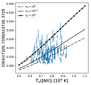
As expected, given that a majority of the are in the low-density limit, we do not observe any correlations between any versus . However, recent studies have suggested that the temperatures obtained from the auroral-to-nebular lines ratios of [O II] and [S II] can be biased upwards due to the presence of density inhomogeneities, even while the average density is underestimated by nebular doublet line [O II] and [S II] diagnostics.
For example, in a sample of 190 high-signal-noise spectra of H ii regions and other photoionized nebulae, Méndez-Delgado et al. (2023b) observed systematically hotter and relative to , similar to what we observe, which they attribute to the presence of density inhomogeneities. The atomic levels responsible for the nebular lines [S II] and [O II], listed in Table 3, have critical densities of order cm-3 which are at least two orders of magnitude lower than the critical densities for the nebular levels of [N II]. In addition, the auroral levels of the same ions have very high critical densities. This makes the auroral-to-nebular temperature diagnostics of and density sensitive above cm-3, and therefore susceptible to biases if there are important contributions to the line flux from gas above that density. The auroral-to-nebular ratio of [N II], however, are not susceptible to such sensitivity until much higher densities.
Both [S II] and [O II] nebular line doublet ratios serve as density diagnostics for densities cm cm-3. Furthermore, because of the bias described above, Méndez-Delgado et al. (2023b) show that at fixed temperature the auroral-to-nebular line ratios for [O II] and [S II] can serve as a density diagnostic over a large range of electron density, cm cm-3. For a uniform density H ii region, the returned from both of these diagnostics should be identical, as long as is within the sensitivity range of the diagnostics. However, in the presence of density inhomogeneities, different density diagnostics can return conflicting values. Even if high density gas clumps make up a small fraction of the gas, such regions can continue to contribute to the auroral line emission while no longer contributing significantly to the nebular lines, since the effects of collisional de-excitation on the nebular lines will reduce their emissivities relative to the auroral lines (Rubin, 1989). Because of this, the nebular [S II] and [O II] lines can reflect the dominant contribution of low-density gas, while the auroral [S II] and [O II] lines will be sensitive to volume of high-density gas (Peimbert, 1971; Rubin, 1989; Méndez-Delgado et al., 2023b).
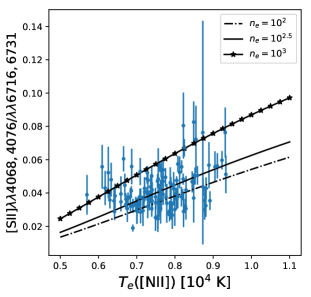
To investigate if the presence of density inhomogeneities could bias our measured and we compare the observed auroral-to-nebular line ratios [O II] and [S II] to those predicted using fixed . We show in Figure 11 the measured [O II]/ and [S II]/ line ratios versus the region’s . We overlay the predicted trends of auroral-to-nebular line ratios calculated using , , and . We see in Figure 11 that under the assumption that , the measured auroral-to-nebular line ratios could be consistent with traced by but with a higher electron density than that returned by [S II] in the low-density limit. This suggests that under inhomogenous conditions, underestimated contributions from cm-3 gas to the nebular [O II] and [S II] lines could bias the density diagnostics and then the use of underestimated densities in temperature calculations for ions with low critical densities like [O II] and [S II] could lead to hotter estimated temperatures inferred from auroral-to-nebular ratios.
7.2.2 Correlations between Temperature Differences and Ionization Parameter
We show in Figures 12 and 13 the comparisons between temperature differences and the ionization parameter, , traced with [S III]/[S II] or [O III]/[O II].
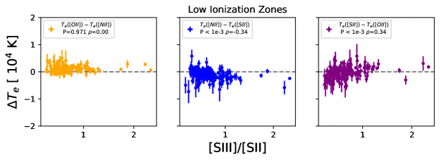
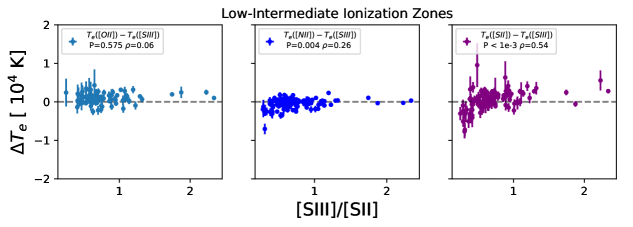
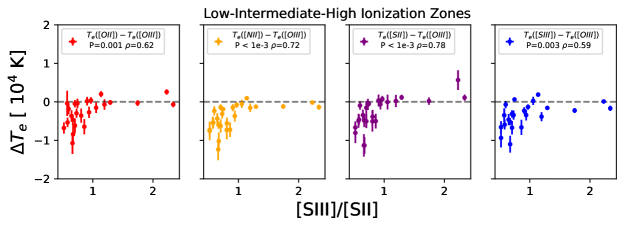
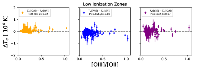
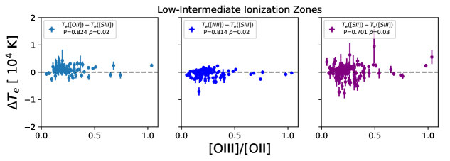
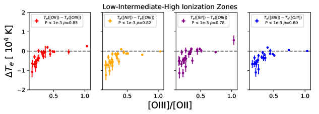
We observe a moderate correlation between (, ) and [S III]/[S II]. The (, ) and (, ) also show correlations with and [S III]/[S II], although these are weaker than the correlation involving (, ). In addition, for all temperature differences with we also observe strong correlations between and [S III]/[S II]. The largest temperature differences are associated with the smallest values of [S III]/[S II]. As [S III]/[S II] increases, converges to . Shown in Figure 13, we present the same temperature differences but using [O III]/[O II] as a tracer for . All the correlations with ionization parameter that do not involve disappear when using [O III]/[O II] as a tracer. The remaining that include show similar correlations as before with ionization parameter when using [O III]/[O II]. In both cases, the largest temperature differences occur at the lowest values of ionization parameter, traced by either [S III]/[S II] or [O III]/[O II].
Our correlations with ionization parameter tracers are similar to the results presented in Yates et al. (2020). When comparing the temperatures of the low and high ionization zone for oxygen, Yates et al. (2020) observed an increase in the / ratio that is anti-correlated with the ratio of (which closely follows the ionization parameter traced by [O III]/[O II]). Our H ii regions are all likely to be in the relatively high metallicity regime, where should be the dominant ionization state of oxygen. Here, the average electron temperature will be best described by the auroral-to-nebular line ratio of [O II] (with caution about density inhomogeneities, as previously noted). Nevertheless, emission from [O III] can still be produced, albeit more weakly, and given the exponential temperature dependence, it will be biased towards hotter gas. Therefore, if there are temperature inhomogenieities, the [O III] temperatures may reflect a small amount of hot, high ionization gas and may not agree with the auroral-to-nebular line ratio of [O II]. Yates et al. (2020) predict that regions with will be dominant, i.e. . Because [O III]/[O II] , we would expect to see the largest deviations in at the lowest [O III]/[O II]. To summarize, Yates et al. (2020) postulate that the differences between hotter high ionization zone temperatures, and the low ionization zone temperature, will increase with decreasing ionization parameter. These trends should in theory also be evident for sulfur, although these correlations were not explored by Yates et al. (2020). Similar trends of temperature differences associated with different ionization states of the gas have been discussed by Berg et al. (2020).
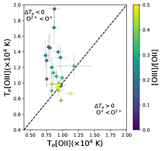
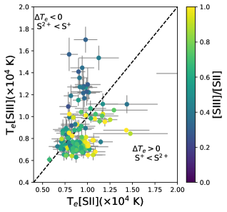
In Figure 14, we plot the – between – and – colored by the value of [O III]/[O II] and [S III]/[S II]. We also annotate the plot according to the schematics from Figure 3 of Yates et al. (2020). For both oxygen and sulfur, the largest ratios of /, where X is either S or O, occur for the lowest values of ionization parameter, as indicated by the value of the line ratio. This suggests we are observing a similar correlation with ionization parameter as postulated by Yates et al. (2020).
If we consider the similarity between our results and Yates et al. (2020) as evidence for correlations between and , then why is it that the correlation between (, ) and traced by [S III]/[S II]is not evident when using [O III]/[O II] as a tracer for ? It might be the case that [S III]/[S II] and [O III]/[O II] do not change with in similar ways, as [S III] and [O III] arise from different ionization zones and conditions. It is possible that density inhomogeneities may be playing a role, both [S II] and [O II] have similar low critical densities, unlike either [S III] and [O III]. It remains unclear why some vs. trends disappear.
7.2.3 Correlations between Temperatures Differences with Stellar Mass and Age
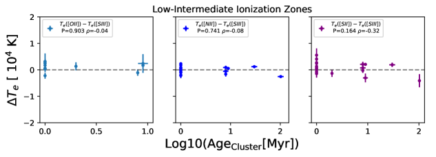
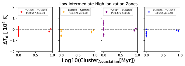
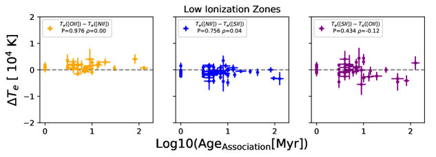
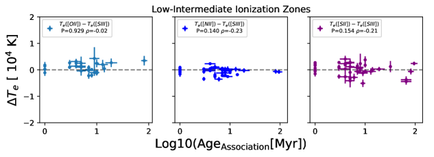
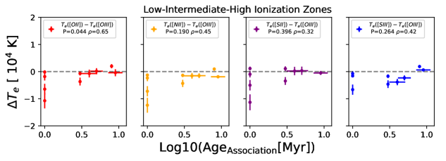
Next we compare temperature differences to stellar mass and ages from compact stellar clusters and associations matched to our H ii regions. As presented in Appendix C Figures 32–34, we find no correlations between with cluster mass, cluster age, or with association age.
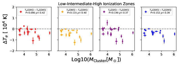
We do observe a weak, positive correlation, between the most reliable indicator without density inhomogeneity issues, (, ) with the association mass in Figure 15. Here we see that is cooler than at lower association mass. As mass increases, we observe that the value of (, ) decreases until becomes larger than . This correlation with association mass spans a small range in temperature differences [,] K with association mass between M⊙ and M⊙.
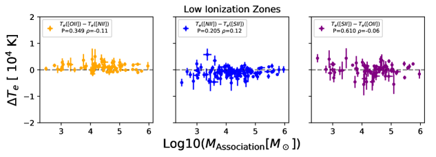
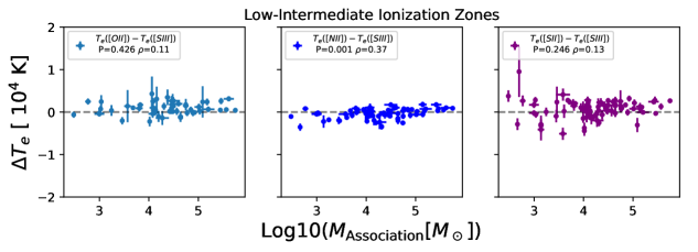
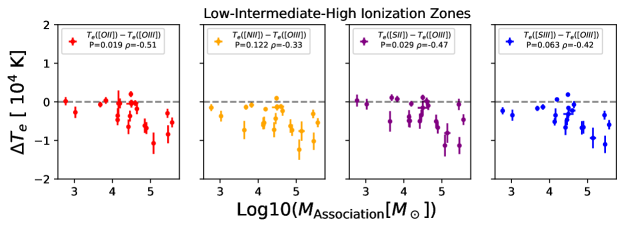
As discussed in Section 6.5, we assigned the largest mass stellar population to the H ii region if the region was matched to more than one association. To see if this choice has any impact on the observed correlation, we plot in Figure 16 the (, ) against the sum of the matched association masses. Using the total masses, we observe a negligible change in the correlation. The p-value is increased from to and the Spearman rank remains unchanged, . To investigate the impact that the error has on the correlation, we construct a distribution Spearman rank coefficients by perturbing each data point by its associated error and remeasuring the correlation. From this we measure a Spearman rank coefficient , indicating that the error has negligible impact on the correlation.
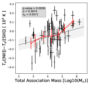
It is possible that the correlation between (, ) and association mass may result from biases introduced by an under-sampling of initial mass function. Similar to our study, Scheuermann et al. (2023) matched the stellar association catalog (Larson et al., 2023) to H ii regions in the Nebular catalog (Kreckel et al., 2019; Groves et al., 2023). Instead of including all masses measured for the associations, which we do in this work, Scheuermann et al. (2023) implement a cut-off and assume masses , as masses below the threshold do not sample the IMF (da Silva et al., 2012). We perform no such cutoff in this study. The correlation between (, ) and correlation includes many regions with masses , where the IMF may not be fully sampled. Despite this, we do not fully dismiss this correlation; however, the effects that undersampling the IMF could have on the correlation with (, ) warrants further investigation with a larger sample size on order to expand the dynamic range of association mass.
7.2.4 Correlations between Temperatures Differences and Molecular Gas Properties
We compare temperature differences to the properties of the molecular gas derived from CO emission measured within the projected boundaries of our sample of H ii regions. For the comparisons to , shown in Figure 35 of Appendix E , and comparisons to , shown in Figure 36 of Appendix E, we observe no correlations with temperature differences between the low, intermediate, and high ionization zones.
We show in Figure 17 the temperature differences compared to the CO velocity dispersion (). We observe a moderate correlation between and (, ). The values of (, ) over the range of is small, only encompassing (, ) from 1000 K to 2000 K. Given the possible correlation with association mass, and this correlation with , we find it intriguing that these correlations between the low and intermediate ionization zone are only seen in (, ). It is possible that the low scatter in – relationship between and in the presence of density inhomogeneities, contrary to the temperatures from [S II] and [O II], allow for better insight into these underlying trends.
We observe that all the correlations of involving and have large, negative, values, but are all insignificant according to their p-values. The high Spearman rank values for the comparisons between and appears to be largely driven by the highest values of . Despite the fact that the correlations are not strong, it is clear that the high regions go along with high CO velocity dispersion.
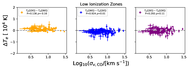
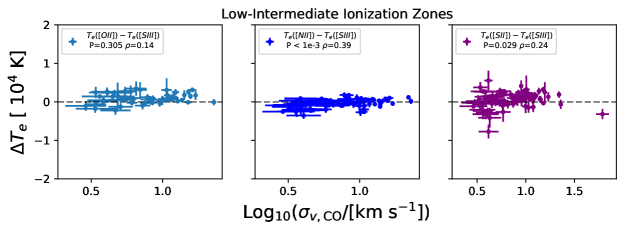
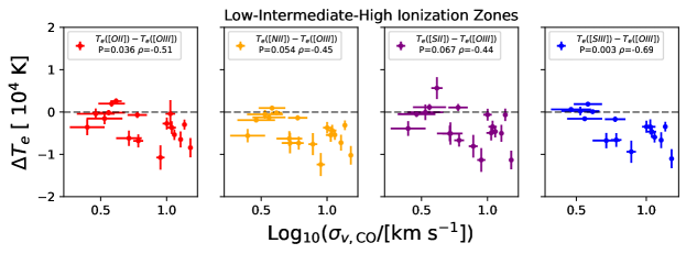
The CO velocity dispersion can be enhanced by low-velocity shocks originating from the interaction of molecular gas with late-time-expansion of supernovae remnants (see Koo et al., 2001; Zhou et al., 2023), as well as from interaction with low-velocity shocks from pressure-radiation driven H ii region expansion (Hill & Hollenbach, 1978; Kothes & Kerton, 2002; Watkins et al., 2023). These low-velocity shocks are also predicted to enhance . Shock modeling have shown that outward expanding low-velocity shocks can create conditions, such as pockets of high post-shock temperature, where the strength of [O III] emission will be enhanced compared to the little to no increase in emission from [O III] (Peimbert et al., 1991; Binette et al., 2012; Méndez-Delgado et al., 2021). The combination of large temperature differences with and high suggests that we may be observing the effects of low-velocity shocks. Motivated by this scenario, we search the H ii regions for evidence of low-velocity shocks in the following section.
7.2.5 Investigating H II Regions for Presence of Low-Velocity Shocks
The correlations of involving the high ionization zone and H ii region properties: [S III]/[S II], [O III]/[O II], and the CO velocity dispersion appears to be driven by the presence of regions with high , high and low . One potential explanation is the presence of low velocity shocks enhancing (Peimbert et al., 1991; Binette et al., 2012; Méndez-Delgado et al., 2021). To test this explanation, we search for evidence of shocks in enhanced optical line ratios and line broadening.
When shocks collide with and compress gas, the ionization parameter of the gas is reduced leading to partially ionized zones of enhanced nebular emission of low-ionization species such as S+ and O relative to H and/or H (Dopita & Sutherland, 1996; Allen et al., 2008). In Figure 18, we show the [S II]/H vs. [O I]/H ratios, color-coded by , for regions with measured [O III]. We find that H ii regions with hotter tend to populate a region with enhanced [S II]/H and [O I]/H ratios which suggests that these regions may host a partially ionized zone due to shocks. We note here that it is possible that harder photons and X-rays produced by X-ray binaries also enhance [S II] and [O I] relative to the Balmer emission (Abolmasov et al., 2007; Grisé et al., 2008). Furthermore, X-rays would provide high energy photons able to boost [O III]. However, lacking the high spatial resolution X-ray imaging of these H ii regions, exploration of X-ray contributions to [O III] emission is beyond the scope of this paper.
Another tracer that may indicate presence of shocks is the He II /H ratio (Allen et al., 2008) though it is also sensitive to the shape of the Lyman continuum below 228 Å (Garnett et al., 1991; Guseva et al., 2000; Allen et al., 2008). Wolf-Rayet (WR) stars are capable of releasing photons able to produce He II . WR stars host stellar winds and can be a source of high energy photons, E eV, capable of doubly ionizing Helium. We measured the He II/H in H ii regions with detections and found that these regions exhibit an average He II /H. This value is within the expected range of He II /H values for H ii regions with WR, 0.04%-7% (Guseva et al., 2000; Thuan & Izotov, 2005; Mayya et al., 2023), and 100 km s-1 shocks, 4%-6% (Allen et al., 2008). We visually inspected the spectra of regions with measured for the characteristic red/blue bump associated with the presence of WR stars. We found the blue bump in only 2 regions with measurable [O III], both of which have K. Nevertheless, the He II /H for the high regions lends evidence that these regions may host shocks or undetected WR stars.
We also searched for kinematic signatures of shocks, but find no clear kinematic evidence. Shocks can imprint asymmetries and/or broad emission near the base of an emission line. We inspected the fit residuals of [O III] in H ii regions with measured and found no evidence of line broadening due to shocks. Next, we inspected the measured line widths of [O III] in these regions. We compared the line-spread-function corrected [O III], as measured by MUSE, velocity dispersion, vs. the CO velocity dispersion, . The line-widths of the optical and CO emission for regions with high are comparable to regions with low, or not detected . Despite this, the absence of these features may only exclude the presence of high-velocity shocks.
If the regions do host low-velocity shocks, then their impact on the line width of the optical emission may be too small to be resolved given the MUSE resolution; km s-1 at Å. The high velocity resolution, of the PHANGS-ALMA data, are more sensitive than MUSE to low-velocity shocks, and are the strongest evidence for their presence in the high H ii regions.
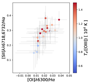
8 Discussion
8.1 Electron Density Inhomogeneities
Similar to the results of Méndez-Delgado et al. (2023b), described in Section 7.2.1, we have found that the presence of electron density inhomogeneities may cause the temperatures measured from [O II] and [S II] to be biased hotter compared to those measured using the [N II] auroral lines.
The critical densities of the nebular lines of [S II] and more so [O II] are low enough that at densities the lines will undergo increased collisional de-excitation. In the presence of density inhomogoneities above this value, the low critical densities will reduce the emissivity of the nebular emission lines from [S II] and [O II]. Because of this, the nebular diagnostic lines of [S II] and [O II] will mainly describe gas component with . This biases the [S II] and [O II] density diagnostic to return electron densities that are lower than the true average density of the H ii region. Since the auroral line critical densities are far higher, this also makes the measured [S II] and [O II] temperatures appear to reflect hotter values.
This effect has been observed in many studies. Densities measured in Milky Way H ii regions (the Orion Nebula, NGC 3604 and NGC 3576) using [Cl III], which is sensitive to greater densities than [S II], routinely show that the [S II] diagnostic returns lower values than [Cl III]. (Pogge et al., 1992; García-Rojas & Esteban, 2007; Núñez-Díaz et al., 2013; Weilbacher et al., 2015). Although densities derived from the [S II] doublet are commonly used in the literature due to their strengths and their insensitivity to dust extinction the [S II] ratio is less sensitive to density than [Cl III], [Ar IV] and [Fe III] diagnostics when cm-3 (see Figure 2 in Méndez-Delgado et al., 2023b). If the equality predicted by photoionization models is true, then the auroral-to-nebular line ratios would suggest a factor of 10 higher density than the [S II] doublet, but neither may well represent the true average density of the region.
Electron density variations may arise from shocks, turbulence, and pre-existing non-uniform structure in the ISM (Hill & Hollenbach, 1978; Dopita & Sutherland, 1996; Allen et al., 2008). Jin et al. (2022) have extended photoionization modeling of ionized nebulae to more complex geometries. Starting with an initial clumpy ISM, ionizing photons will pass through diffuse regions more readily than denser clumps. The resulting photoionized region will exhibit fluctuations in density and irregular geometry as opposed to a uniform density and spherical morphology. The ionization parameter in the dense clumps will be relatively lower than other regions of the nebulae due to the increased density. At these locations, the emission of low-ionization species, including [S II] and [O II], will be enhanced compared to higher ionization species. Due to the higher critical densities of the auroral lines of these ions, the emissivity of the auroral lines will be greater than those of the nebular lines in the high-density portion the nebula. In this scenario, the nebular density diagnostics can return an average density that traces the low-density portion of the nebula. In doing so, the value of returned by the nebular diagnostics may inaccurately describe the ionizing conditions of the high-density clumps where the auroral line emissivities are greater than the nebular lines, and overestimate [S II] temperatures.
Density inhomogeneities have been reported in studies of highly resolved local HII regions like Orion where the inhomogeneities can be spatially resolved (Baldwin et al., 1991; Pogge et al., 1992; Weilbacher et al., 2015; McLeod et al., 2016; O’Dell et al., 2017). Weilbacher et al. (2015) mapped the spatial variation of density in the Orion nebulae and found variations of density between 500 cm-3 and in excess of 10,000 cm-3. A maximum of 25,000 cm-3 is measured using [Cl III] at the location of the ionization front in the “Orion S” area. Density inhomogeneities, associated with turbulence driven velocity fluctuations, have been invoked as one mechanism to generate surface brightness fluctuations within the Orion Nebula (Kainulainen et al., 2017).
The Orion Nebula is not particularly comparable to the H ii regions studied here due to the difference in scales (i.e., Orion is more compact) and resolution. A subset of our H ii regions, as shown in the comparison between the MUSE H ii regions mask in Appendix C, are unresolved clusters of individual regions. Measurements of density inhomogeneities using density diagnostics besides the nebular [O II] and [S II] doublets for extragalactic H ii regions that more closely match our sample are rare and require deep, high spectra (Méndez-Delgado et al., 2023b). One consequence of the lack of different diagnostics is that many studies will often assume a fixed density of cm-3 when either [S II], or [O II], return a density in the low-density limit (e.g. Kreckel et al., 2019). Studies using mid-infrared observations have shown this latter assumption could be incorrect, as densities up to have been measured using the [S III]m density diagnostic (see Rubin et al., 2016), and indicate that density inhomogeneities are present in extra-galactic H ii regions.
The consistency of auroral-to-nebular ratios with cm-3 assuming in Figure 11 supports this picture that inhomogeneities must be considered when deriving temperatures from the [O II] and [S II]. As a result, we consider a more reliable indicator of the low-ionization zone temperature due to its relative insensitivity to density.
8.2 and as Accurate Tracers of HII Region Temperatures
The low scatter and overlap with literature – trends between and in Figure 9 indicate that these temperatures may be optimal tracers of H ii region temperatures, more so than , and .
The tight relationship between and measured in this study has been observed in the some studies (Berg et al., 2015; Croxall et al., 2016; Berg et al., 2020; Zurita et al., 2021), especially for the coolest, highest metallicity regions. It is this metallicity regime where it is expected that the widely used [O III] auroral line temperatures will be most difficult to observe, as evident in the small number of measurements relative to and measurements in our study. We showed that (, ) does have a small correlation with the H ii region’s matched stellar association mass and molecular gas velocity dispersion, though, the magnitude of the temperature difference for these correlations span a narrow range of , indicative that and change in similar ways with H ii region properties, unlike correlations with [O III] temperatures, which show very large differences with other ionization zones. In fact, it is tantalizing that the observed correlations between the low and intermediate ionization zones mostly involve and . These underlying trends may be more easily revealed due to the well behaved relationship between and in – relations in the presence of inhomogeneous conditions. Unlike [O II] and [S II], [N II] is less sensitive to density inhomogeneities due to the the higher critical density of the atomic levels involved. The [N II] auroral line is also less contaminated by blended emission (Berg et al., 2020; Méndez-Delgado et al., 2023b). Additionally,temperatures from [N II] were shown to strongly correlate with O II RL temperatures measured for the low-ionization zone Méndez-Delgado et al. (2023a).
Judged from Oxygen CEL and RL temperatures, the high ionization zone is expected to be most affected by temperature fluctuations due to its proximity to sources of feedback (Méndez-Delgado et al., 2023a). To what degree the intermediate ionization zone temperatures are affected is unclear (Méndez-Delgado et al., 2023b). In Figure 9 we showed that the relationship between and generally follow trends predicted from photoionization models (Morisset, 2009; Vale Asari et al., 2016) with . The overlap with our data indicates that may be minimally affected by temperature inhomogeneities. Díaz & Zamora (2022) provide additional arguments for the use of over , including: 1) the emission lines of [S III] have a lower exponential dependence on electron temperature and 2) because [S III] overlaps gas volumes containing both and that can be representative of the entire H ii region.
The behaviour between and across several H ii region properties and photoionization model – suggests prioritization of [N II] and [S III] temperatures over those from [O II], [S II], and [O III] for regions in our sample. We will test this recommendation in an upcoming work, where we will compare “direct” metallicities, derived using [N II] and [S III] temperatures, to several calibrated methods (Rickards Vaught et al., in prep).
8.3 The High-Ionization Zone Temperature Excess
We found H ii regions with high , enhanced velocity dispersion in the surrounding molecular gas and low-ionization parameter. We investigated these H ii regions for enhanced low-ionization species emission line ratios [S II]/H, [O I]/H and the high-ionization ratio He II/H. We found that the high regions exhibited enhanced low-ionization line ratios suggestive of shock ionization (or possibly X-ray ionization). We also found that the He II/H ratios for these regions are within the range of those expected from shock velocities km s-1 (Allen et al., 2008) and/or WR stars (Guseva et al., 2000; Thuan & Izotov, 2005; Mayya et al., 2023), though we only find characteristic red/blue bumps associated with the presence of WR stars, in 2 H ii regions neither of which had elevated . Absent the WR signatures, we are motivated to explore shocks as enhancers of the [O III] temperature.
We did not find any kinematic signatures of shocks in the optical emission line profiles. We determine that if shocks are present and broadening the CO emission, then the shock velocities are too low to be resolved by the MUSE spectral resolution. Either way, high-velocity shocks are not expected to effectively boost (Méndez-Delgado et al., 2021). Despite the uncertainty in whether shocks are present in the high [O III] temperature regions, we can discuss the plausibility that low-velocity shocks are the cause for excess .
8.3.1 Shock-enhanced [O III] Temperature
Low velocity, 100 km s-1, shocks can increase [O III] while leaving [O III] unchanged (Peimbert et al., 1991; Binette et al., 2012; Méndez-Delgado et al., 2021). For a sample of giant H ii regions, Binette et al. (2012) measured up to 6000 K higher than in regions with K. To explore if shocks were boosting their [O III] temperatures relative to [S III], they model outward expanding shocks, mimicking those generated by stellar winds, by combining shockphotoionization models, with increasing shock velocities (analogous to increasing the post-shock temperature from 1.6 K to 7.2 K) between 20 and 60 km s-1. Additionally, the models span 5 different metallicities between Z0.01 Z⊙ to Z1.6 Z⊙. Comparing the average properties of between the lowest and highest shock velocity models, Binette et al. (2012) found that mean doubly ionized fraction of oxygen, / , decreases while at the same time leaving the doubly ionized fraction of sulfur, /, unchanged. The imbalance the ionization fraction between oxygen and sulfur means that hotter, post-shock gas contributes proportionally more to the observed [O III] emission than [S III]. Because of the exponential sensitivity to temperature, the [O III] auroral line will be enhanced, tracing the hotter post-shock temperature rather than the local photoionized nebula temperature returned by . Furthermore, the highest metallicity models show the largest temperature differences between and , up to K. Although this difference is 3000 K lower than our largest measured (, ), a complete understanding of the degree of enhancement of [O III] with velocity shocks require more complex 3D hydro-dynamical simulations (Binette et al., 2012). Despite this, one extreme example of shock impact on electron temperatures was observed in the outflow of the H ii region Sh 2-129 (Corradi et al., 2014). This outflow, with velocity , exhibits K and K. Much larger than observed in this study.
It has also been shown that shocks driven by pressure–radiation H ii region expansion, and SNR, impact the surrounding cold molecular and ionized gas. If the velocity of the expansion is greater than the sound speed ionized gas km s-1, a layer of shocked H gas will form in-between the expanding ionization front and a surrounding molecular gas (Hill & Hollenbach, 1978; Kothes & Kerton, 2002; Tremblin et al., 2014; Watkins et al., 2023). The impact of shock interaction with molecular gas has been studied in 18 galaxies observed as part of PHANGS-ALMA (Leroy et al., 2021a, b), where Watkins et al. (2023) identified hundreds of super bubbles (i.e. pockets of expanding gas arising as byproducts of feedback). The superbubbles were identified using spatial correspondence between CO shells and stellar populations contained in PHANGS-HST catalogs (Lee et al., 2022; Thilker et al., 2022; Larson et al., 2023). Due to the ALMA spatial resolution (50–150 pc), Watkins et al. (2023) measured the expansion velocity only for the largest superbubbles. Assuming the CO expansion velocity is equal to the shock velocity, Watkins et al. (2023) measure the velocity of the approaching/receding CO shells and determine an average, line-of-sight, expansion velocity of 9.8 4.3 km s-1. Although this value is similar to the sound speed of ionized gas, superbubbles exhibit asymmetries in their morphology, and the velocity can potentially reach up to a few tens of km s-1 depending on the conditions of the gas, source or energy injection, and age (Watkins et al., 2023). 1D models indicate that, at minimum, H ii regions exhibit expansion speeds of a few km s-1 (Tremblin et al., 2014). This suggests that H ii regions expand with a large range of velocities.
As for ionized gas, Egorov et al. (2023) identify in the PHANGS-MUSE galaxies more than 1400 regions of ionized gas with elevated intrinsic H velocity dispersions km s-1, and, under the assumption that these regions are undergoing expansion, Egorov et al. (2023) infer expansion velocities between 10–40 km s-1 (see also Egorov et al., 2014, 2017; Cosens et al., 2022). The ubiquity of H ii region expansion, as well as their effects on the surrounding molecular gas, make them good candidates for drivers of low-velocity shocks capable of boosting [O III] temperatures.
8.3.2 Temperature Inhomogeneities
Temperature fluctuations within H ii regions are another potential explanation for the high [O III] temperature. As discussed in Section 1, RL emissivities have a linear sensitivity to temperature rather than the exponential sensitivity of CELs. In the presence of temperature fluctuations CELs will return higher estimates of temperature. Méndez-Delgado et al. (2023a) have recently shown that differences between [O III] and [N II] temperatures are strongly correlated with the temperature fluctuations parameter, , of the highly ionized gas. This suggests that is likely to overestimate the representative H ii region temperature. The observed excess in are likely to be produced by phenomena other than those commonly observed in H ii regions. Simple models from Binette et al. (2012) and the observations from Méndez-Delgado et al. (2023a) show that the effect from is more pronounced in lower-metallicity/high ionization parameter regions. Furthermore, the temperature excess relative to the other ionization zones is too large in our observations to be caused solely by inhomogeneities. Using our measured (, ), we can infer from Méndez-Delgado et al. (2023a) that for (, ) K. These values are much higher than what has been observed for nearby H ii regions (Peña-Guerrero et al., 2012; Binette et al., 2012; Méndez-Delgado et al., 2023a). Even in the presence of classical temperature inhomogeneities, a secondary effect would also need to be included to explain our [O III] temperatures.
8.3.3 Potential Observation Bias
Another possibility is that the high [O III] temperatures are statistical outliers. The galaxies in our sample exhibit strong line oxygen abundances 8.3 (Kreckel et al., 2019). Because electron temperature is anti-correlated to the metallicity of the gas, the [O III] temperatures for these galaxies are expected to be low. For [O III] to be detectable, the temperature would need to be high, otherwise, we would likely not detect the auroral line. [O III] temperatures from a lower-metallicity sample may be compatible with photoionization models and – relations. Finally, Rola & Pelat (1994) have shown that emission line measurements with S/N can potentially overestimate the true intensity by . The average S/N [O III] measured from our sample is . Nevertheless, why we would measure high [O III], even after removal of [Fe II] contamination, that also exhibit enhanced molecular gas velocity dispersions is difficult to explain purely with statistical outliers.
9 Conclusion
We presented combined KCWI and MUSE observations of the [N II], [O II], [S II], [O III], and [S III] auroral lines in a sample of 421 H ii regions in 7 nearby galaxies. We compared the derived electron temperatures and temperature differences between multiple H ii region ionization zones to several H ii region properties such as electron density, ionization parameter, molecular gas velocity dispersion, stellar mass and age obtained from PHANGS observations. We found that:
-
•
Temperatures obtained from [S II] and [O II] are consistent with being overestimated due to the presence of density inhomogeneities in the H ii regions. Because of these potential biases, we recommend the use [N II] temperatures to trace the low ionization zone.
-
•
We found that the [N II] and [S III] temperatures exhibited the lowest scatter of the – relations and follow trends predicted from photoionization models. The well-behaved relationship between [N II] and [S III], even in potentially inhomogeneous conditions, may be better tracing the underlying H ii region temperatures. Together, this suggests prioritization of [N II] and [S III] temperatures for metallicity determinations.
-
•
We observed a subset of H ii regions with high [O III] temperatures that do not agree with the cooler temperatures measured in the low and intermediate ionization zones. We found that the regions with high [O III] temperature tended to have enhanced molecular gas velocity dispersion and lower ionization parameter than those regions with [O III] temperatures that were in better agreement with other ionization zones. These regions also showed enhanced [S II]/H, [O I]/H, and He II/H ratios indicating the presence of secondary ionization sources (e.g. shocks, Wolf-Rayet and X-ray binary stars). Absent direct detection of shocks, we explored whether or not shocks are able to both enhance and CO velocity dispersion. We found that low-velocity shocks are a plausible explanation for the observed [O III] temperatures and CO velocity dispersions. However, disentangling the effects of shocks from possible contributions to [O III] temperatures by harder ionization sources such as Wolf-Rayet stars or X-ray binaries require further investigation.
-
•
We also explored temperature inhomogenities and observational uncertainties as causes for the high [O III] temperatures. We found that the degree of temperature inhomogeneity that would be required to produce the difference between high [O III] temperatures and those of the low and intermediate ionization zone are larger than what has been observed in most star-forming regions. Furthermore, if the regions with high [O III] temperatures are statistical outliers leading to overestimated temperatures, we lack an explanation as to why these temperatures would correlate with high molecular gas velocity dispersion.
In a follow-up paper, Rickards Vaught et al. (in prep), We will test temperature recommendations for measuring “direct” metallicities using our full set of measured auroral line temperatures. This work, along with the PHANGS-MUSE survey, demonstrate the power of integral field spectrographs on 10m class telescopes for measuring faint auroral emission lines from large samples of H ii regions in nearby galaxies. Future efforts with deeper observations or expanded samples will be critical for further elucidating the temperature and ionization behavior of these regions, particularly as [O III] and other faint lines are now being routinely detected in galaxies at high redshift with JWST and used in metallicity determinations.
Acknowledgements
The data presented herein were obtained at the W. M. Keck Observatory, which is operated as a scientific partnership among the California Institute of Technology, the University of California and the National Aeronautics and Space Administration. The Observatory was made possible by the generous financial support of the W. M. Keck Foundation. The authors wish to recognize and acknowledge the very significant cultural role and reverence that the summit of Maunakea has always had within the indigenous Hawaiian community. We are most fortunate to have the opportunity to conduct observations from this mountain. We also wish to thank all the Keck Observatory staff, including Gregg Doppman, Luca Rizzi, Sheery Yeh, and Rosalie McGurk for observational support.
This research is also based on observations collected at the European Southern Observatory under ESO programmes 094.C-0623 (PI: Kreckel), 095.C-0473, 098.C-0484 (PI: Blanc), 1100.B-0651 (PHANGS-MUSE; PI: Schinnerer), as well as 094.B-0321 (MAGNUM; PI: Marconi), 099.B-0242, 0100.B-0116, 098.B-0551 (MAD; PI: Carollo) and 097.B-0640 (TIMER; PI: Gadotti).
RRV and KS acknowledge funding support from National Science Foundation Award No. 1816462. FB acknowledges funding from the INAF Fundamental Astrophysics 2022 program. RRV wishes to thank Jonah Gannon, and Maren Consens for fruitful discussions on reducing the KCWI data. RRV would also like to acknowledge discussions with JEM-D, KK, OVE which greatly improved the manuscript. KK, JEM-D and OVE gratefully acknowledge funding from the Deutsche Forschungsgemeinschaft (DFG, German Research Foundation) in the form of an Emmy Noether Research Group (grant number KR4598/2-1, PI Kreckel). KG is supported by the Australian Research Council through the Discovery Early Career Researcher Award (DECRA) Fellowship (project number DE220100766) funded by the Australian Government. KG is supported by the Australian Research Council Centre of Excellence for All Sky Astrophysics in 3 Dimensions (ASTRO 3D), through project number CE170100013. JN acknowledges funding from the European Research Council (ERC) under the European Union’s Horizon 2020 research and innovation programme (grant agreement No. 694343). RSK acknowledges funding from the European Research Council via the ERC Synergy Grant “ECOGAL” (project ID 855130), from the German Excellence Strategy via the Heidelberg Cluster of Excellence (EXC 2181 - 390900948) “STRUCTURES”, and from the German Ministry for Economic Affairs and Climate Action in project “MAINN” (funding ID 50OO2206). He also thanks for computing resources provided by The Länd and DFG through grant INST 35/1134-1 FUGG and for data storage at SDS@hd through grant INST 35/1314-1 FUGG. G.A.B. acknowledges the support from the ANID Basal project FB210003.
This research made use of Montage. It is funded by the National Science Foundation under Grant Number ACI-1440620, and was previously funded by the National Aeronautics and Space Administration’s Earth Science Technology Office, Computation Technologies Project, under Cooperative Agreement Number NCC5-626 between NASA and the California Institute of Technology. This research has made use of NASA’s Astrophysics Data System. This research made use of Astropy, a community-developed core Python package for Astronomy (Astropy Collaboration et al., 2013), as well as substantial use of the nebular diagnostics toolkit Pyneb (Luridiana et al., 2015).
References
- Abazajian et al. (2003) Abazajian, K., Adelman-McCarthy, J. K., Agüeros, M. A., et al. 2003, AJ, 126, 2081, doi: 10.1086/378165
- Abolmasov et al. (2007) Abolmasov, P., Fabrika, S., Sholukhova, O., & Afanasiev, V. 2007, Astrophysical Bulletin, 62, 36, doi: 10.1134/S199034130701004X
- Allen et al. (2008) Allen, M. G., Groves, B. A., Dopita, M. A., Sutherland, R. S., & Kewley, L. J. 2008, ApJS, 178, 20, doi: 10.1086/589652
- Anand et al. (2021) Anand, G. S., Lee, J. C., Van Dyk, S. D., et al. 2021, MNRAS, 501, 3621, doi: 10.1093/mnras/staa3668
- Arellano-Córdova & Rodríguez (2020) Arellano-Córdova, K. Z., & Rodríguez, M. 2020, MNRAS, 497, 672, doi: 10.1093/mnras/staa1759
- Astropy Collaboration et al. (2013) Astropy Collaboration, Robitaille, T. P., Tollerud, E. J., et al. 2013, A&A, 558, A33, doi: 10.1051/0004-6361/201322068
- Bacon et al. (2010) Bacon, R., Accardo, M., Adjali, L., et al. 2010, in Society of Photo-Optical Instrumentation Engineers (SPIE) Conference Series, Vol. 7735, Ground-based and Airborne Instrumentation for Astronomy III, ed. I. S. McLean, S. K. Ramsay, & H. Takami, 773508, doi: 10.1117/12.856027
- Baldwin et al. (1991) Baldwin, J. A., Ferland, G. J., Martin, P. G., et al. 1991, ApJ, 374, 580, doi: 10.1086/170146
- Baldwin et al. (1981) Baldwin, J. A., Phillips, M. M., & Terlevich, R. 1981, PASP, 93, 5, doi: 10.1086/130766
- Belfiore et al. (2019) Belfiore, F., Westfall, K. B., Schaefer, A., et al. 2019, AJ, 158, 160, doi: 10.3847/1538-3881/ab3e4e
- Belfiore et al. (2022) Belfiore, F., Santoro, F., Groves, B., et al. 2022, A&A, 659, A26, doi: 10.1051/0004-6361/202141859
- Berg et al. (2020) Berg, D. A., Pogge, R. W., Skillman, E. D., et al. 2020, ApJ, 893, 96, doi: 10.3847/1538-4357/ab7eab
- Berg et al. (2015) Berg, D. A., Skillman, E. D., Croxall, K. V., et al. 2015, ApJ, 806, 16, doi: 10.1088/0004-637X/806/1/16
- Binette et al. (2012) Binette, L., Matadamas, R., Hägele, G. F., et al. 2012, A&A, 547, A29, doi: 10.1051/0004-6361/201219515
- Blanc et al. (2015) Blanc, G. A., Kewley, L., Vogt, F. P. A., & Dopita, M. A. 2015, ApJ, 798, 99, doi: 10.1088/0004-637X/798/2/99
- Bresolin et al. (2012) Bresolin, F., Kennicutt, R. C., & Ryan-Weber, E. 2012, ApJ, 750, 122, doi: 10.1088/0004-637X/750/2/122
- Calzetti et al. (2015) Calzetti, D., Lee, J. C., Sabbi, E., et al. 2015, AJ, 149, 51, doi: 10.1088/0004-6256/149/2/51
- Campbell et al. (1986) Campbell, A., Terlevich, R., & Melnick, J. 1986, MNRAS, 223, 811, doi: 10.1093/mnras/223.4.811
- Cappellari (2017) Cappellari, M. 2017, MNRAS, 466, 798, doi: 10.1093/mnras/stw3020
- Cappellari & Emsellem (2004) Cappellari, M., & Emsellem, E. 2004, PASP, 116, 138, doi: 10.1086/381875
- Casini & de Wijn (2014) Casini, R., & de Wijn, A. G. 2014, Journal of the Optical Society of America A, 31, 2002, doi: 10.1364/JOSAA.31.002002
- Congiu et al. (2023) Congiu, E., Blanc, G. A., Belfiore, F., et al. 2023, A&A, 672, A148, doi: 10.1051/0004-6361/202245153
- Corradi et al. (2014) Corradi, R. L. M., Grosso, N., Acker, A., Greimel, R., & Guillout, P. 2014, A&A, 570, A105, doi: 10.1051/0004-6361/201322718
- Cosens et al. (2022) Cosens, M., Wright, S. A., Murray, N., et al. 2022, ApJ, 929, 74, doi: 10.3847/1538-4357/ac52f3
- Croxall et al. (2016) Croxall, K. V., Pogge, R. W., Berg, D. A., Skillman, E. D., & Moustakas, J. 2016, ApJ, 830, 4, doi: 10.3847/0004-637X/830/1/4
- Curti et al. (2017) Curti, M., Cresci, G., Mannucci, F., et al. 2017, MNRAS, 465, 1384, doi: 10.1093/mnras/stw2766
- da Silva et al. (2012) da Silva, R. L., Fumagalli, M., & Krumholz, M. 2012, ApJ, 745, 145, doi: 10.1088/0004-637X/745/2/145
- Díaz & Zamora (2022) Díaz, Á. I., & Zamora, S. 2022, MNRAS, 511, 4377, doi: 10.1093/mnras/stac387
- Dopita & Sutherland (1996) Dopita, M. A., & Sutherland, R. S. 1996, ApJS, 102, 161, doi: 10.1086/192255
- Dors et al. (2011) Dors, O. L., J., Krabbe, A., Hägele, G. F., & Pérez-Montero, E. 2011, MNRAS, 415, 3616, doi: 10.1111/j.1365-2966.2011.18978.x
- Draine (2011) Draine, B. T. 2011, Physics of the Interstellar and Intergalactic Medium
- Egorov et al. (2017) Egorov, O. V., Lozinskaya, T. A., Moiseev, A. V., & Shchekinov, Y. A. 2017, MNRAS, 464, 1833, doi: 10.1093/mnras/stw2367
- Egorov et al. (2014) Egorov, O. V., Lozinskaya, T. A., Moiseev, A. V., & Smirnov-Pinchukov, G. V. 2014, MNRAS, 444, 376, doi: 10.1093/mnras/stu1369
- Egorov et al. (2023) Egorov, O. V., Kreckel, K., Glover, S. C. O., et al. 2023, arXiv e-prints, arXiv:2307.10277, doi: 10.48550/arXiv.2307.10277
- Emsellem et al. (2022) Emsellem, E., Schinnerer, E., Santoro, F., et al. 2022, A&A, 659, A191, doi: 10.1051/0004-6361/202141727
- Esteban et al. (2004) Esteban, C., Peimbert, M., García-Rojas, J., et al. 2004, MNRAS, 355, 229, doi: 10.1111/j.1365-2966.2004.08313.x
- Fitzpatrick (1999) Fitzpatrick, E. L. 1999, PASP, 111, 63, doi: 10.1086/316293
- Freedman et al. (2001) Freedman, W. L., Madore, B. F., Gibson, B. K., et al. 2001, ApJ, 553, 47, doi: 10.1086/320638
- Froese Fischer & Tachiev (2004) Froese Fischer, C., & Tachiev, G. 2004, Atomic Data and Nuclear Data Tables, 87, 1, doi: 10.1016/j.adt.2004.02.001
- Froese Fischer et al. (2006) Froese Fischer, C., Tachiev, G., & Irimia, A. 2006, Atomic Data and Nuclear Data Tables, 92, 607, doi: 10.1016/j.adt.2006.03.001
- García-Rojas & Esteban (2007) García-Rojas, J., & Esteban, C. 2007, ApJ, 670, 457, doi: 10.1086/521871
- Garnett (1992) Garnett, D. R. 1992, AJ, 103, 1330, doi: 10.1086/116146
- Garnett et al. (1991) Garnett, D. R., Kennicutt, Robert C., J., Chu, Y.-H., & Skillman, E. D. 1991, ApJ, 373, 458, doi: 10.1086/170065
- Grasha et al. (2019) Grasha, K., Calzetti, D., Adamo, A., et al. 2019, MNRAS, 483, 4707, doi: 10.1093/mnras/sty3424
- Grasha et al. (2022) Grasha, K., Chen, Q. H., Battisti, A. J., et al. 2022, ApJ, 929, 118, doi: 10.3847/1538-4357/ac5ab2
- Grisé et al. (2008) Grisé, F., Pakull, M. W., Soria, R., et al. 2008, A&A, 486, 151, doi: 10.1051/0004-6361:200809557
- Groves et al. (2023) Groves, B., Kreckel, K., Santoro, F., et al. 2023, MNRAS, 520, 4902, doi: 10.1093/mnras/stad114
- Guseva et al. (2000) Guseva, N. G., Izotov, Y. I., & Thuan, T. X. 2000, ApJ, 531, 776, doi: 10.1086/308489
- Hernandez et al. (2013) Hernandez, A. K., Wakker, B. P., Benjamin, R. A., et al. 2013, ApJ, 777, 19, doi: 10.1088/0004-637X/777/1/19
- Hill & Hollenbach (1978) Hill, J. K., & Hollenbach, D. J. 1978, ApJ, 225, 390, doi: 10.1086/156501
- Ho et al. (2016) Ho, I. T., Medling, A. M., Groves, B., et al. 2016, Ap&SS, 361, 280, doi: 10.1007/s10509-016-2865-2
- Ho et al. (2017) Ho, I. T., Seibert, M., Meidt, S. E., et al. 2017, ApJ, 846, 39, doi: 10.3847/1538-4357/aa8460
- Jacobs et al. (2009) Jacobs, B. A., Rizzi, L., Tully, R. B., et al. 2009, AJ, 138, 332, doi: 10.1088/0004-6256/138/2/332
- Jin et al. (2022) Jin, Y., Kewley, L. J., & Sutherland, R. S. 2022, ApJ, 934, L8, doi: 10.3847/2041-8213/ac80f3
- Kainulainen et al. (2017) Kainulainen, J., Stutz, A. M., Stanke, T., et al. 2017, A&A, 600, A141, doi: 10.1051/0004-6361/201628481
- Kaler et al. (1976) Kaler, J. B., Aller, L. H., Czyzak, S. J., & Epps, H. W. 1976, ApJS, 31, 163, doi: 10.1086/190379
- Kauffmann et al. (2003) Kauffmann, G., Heckman, T. M., Tremonti, C., et al. 2003, MNRAS, 346, 1055, doi: 10.1111/j.1365-2966.2003.07154.x
- Kennicutt et al. (2003) Kennicutt, Robert C., J., Bresolin, F., & Garnett, D. R. 2003, ApJ, 591, 801, doi: 10.1086/375398
- Kennicutt & Garnett (1996) Kennicutt, Robert C., J., & Garnett, D. R. 1996, ApJ, 456, 504, doi: 10.1086/176675
- Kewley & Dopita (2002) Kewley, L. J., & Dopita, M. A. 2002, ApJS, 142, 35, doi: 10.1086/341326
- Kewley & Ellison (2008) Kewley, L. J., & Ellison, S. L. 2008, ApJ, 681, 1183, doi: 10.1086/587500
- Kewley et al. (2001) Kewley, L. J., Heisler, C. A., Dopita, M. A., & Lumsden, S. 2001, ApJS, 132, 37, doi: 10.1086/318944
- Kisielius et al. (2009) Kisielius, R., Storey, P. J., Ferland, G. J., & Keenan, F. P. 2009, MNRAS, 397, 903, doi: 10.1111/j.1365-2966.2009.14989.x
- Koo et al. (2001) Koo, B.-C., Rho, J., Reach, W. T., Jung, J., & Mangum, J. G. 2001, ApJ, 552, 175, doi: 10.1086/320442
- Kothes & Kerton (2002) Kothes, R., & Kerton, C. R. 2002, A&A, 390, 337, doi: 10.1051/0004-6361:20020671
- Kourkchi et al. (2020) Kourkchi, E., Courtois, H. M., Graziani, R., et al. 2020, AJ, 159, 67, doi: 10.3847/1538-3881/ab620e
- Kourkchi & Tully (2017) Kourkchi, E., & Tully, R. B. 2017, ApJ, 843, 16, doi: 10.3847/1538-4357/aa76db
- Kreckel et al. (2019) Kreckel, K., Ho, I. T., Blanc, G. A., et al. 2019, ApJ, 887, 80, doi: 10.3847/1538-4357/ab5115
- Kreckel et al. (2020) —. 2020, MNRAS, 499, 193, doi: 10.1093/mnras/staa2743
- Kreckel et al. (2022) Kreckel, K., Egorov, O. V., Belfiore, F., et al. 2022, A&A, 667, A16, doi: 10.1051/0004-6361/202243858
- Larson et al. (2023) Larson, K. L., Lee, J. C., Thilker, D. A., et al. 2023, MNRAS, 523, 6061, doi: 10.1093/mnras/stad1600
- Law et al. (2016) Law, D. R., Cherinka, B., Yan, R., et al. 2016, AJ, 152, 83, doi: 10.3847/0004-6256/152/4/83
- Lee et al. (2022) Lee, J. C., Whitmore, B. C., Thilker, D. A., et al. 2022, ApJS, 258, 10, doi: 10.3847/1538-4365/ac1fe5
- Leroy et al. (2021a) Leroy, A. K., Schinnerer, E., Hughes, A., et al. 2021a, ApJS, 257, 43, doi: 10.3847/1538-4365/ac17f3
- Leroy et al. (2021b) Leroy, A. K., Hughes, A., Liu, D., et al. 2021b, ApJS, 255, 19, doi: 10.3847/1538-4365/abec80
- Luridiana et al. (2015) Luridiana, V., Morisset, C., & Shaw, R. A. 2015, A&A, 573, A42, doi: 10.1051/0004-6361/201323152
- Makarov et al. (2014) Makarov, D., Prugniel, P., Terekhova, N., Courtois, H., & Vauglin, I. 2014, A&A, 570, A13, doi: 10.1051/0004-6361/201423496
- Mayya et al. (2023) Mayya, Y. D., Plat, A., Gómez-González, V. M. A., et al. 2023, MNRAS, 519, 5492, doi: 10.1093/mnras/stad017
- McLeod et al. (2016) McLeod, A. F., Weilbacher, P. M., Ginsburg, A., et al. 2016, MNRAS, 455, 4057, doi: 10.1093/mnras/stv2617
- Méndez-Delgado et al. (2022) Méndez-Delgado, J. E., Esteban, C., García-Rojas, J., & Henney, W. J. 2022, MNRAS, 514, 744, doi: 10.1093/mnras/stac1300
- Méndez-Delgado et al. (2021) Méndez-Delgado, J. E., Esteban, C., García-Rojas, J., et al. 2021, MNRAS, 502, 1703, doi: 10.1093/mnras/stab068
- Méndez-Delgado et al. (2023a) Méndez-Delgado, J. E., Esteban, C., García-Rojas, J., Kreckel, K., & Peimbert, M. 2023a, Nature, 618, 249, doi: 10.1038/s41586-023-05956-2
- Méndez-Delgado et al. (2023b) Méndez-Delgado, J. E., Esteban, C., García-Rojas, J., et al. 2023b, MNRAS, 523, 2952, doi: 10.1093/mnras/stad1569
- Mendoza et al. (2023) Mendoza, C., Méndez-Delgado, J. E., Bautista, M., García-Rojas, J., & Morisset, C. 2023, Atoms, 11, 63, doi: 10.3390/atoms11040063
- Morisset (2009) Morisset, C. 2009, Mem. Soc. Astron. Italiana, 80, 397, doi: 10.48550/arXiv.0909.3313
- Morrissey et al. (2018) Morrissey, P., Matuszewski, M., Martin, D. C., et al. 2018, ApJ, 864, 93, doi: 10.3847/1538-4357/aad597
- Nicholls et al. (2020) Nicholls, D. C., Kewley, L. J., & Sutherland, R. S. 2020, PASP, 132, 033001, doi: 10.1088/1538-3873/ab6818
- Núñez-Díaz et al. (2013) Núñez-Díaz, M., Esteban, C., & Mesa-Delgado, A. 2013, in Highlights of Spanish Astrophysics VII, ed. J. C. Guirado, L. M. Lara, V. Quilis, & J. Gorgas, 594–599
- Nugent et al. (2006) Nugent, P., Sullivan, M., Ellis, R., et al. 2006, ApJ, 645, 841, doi: 10.1086/504413
- O’Dell et al. (2017) O’Dell, C. R., Ferland, G. J., & Peimbert, M. 2017, MNRAS, 464, 4835, doi: 10.1093/mnras/stw2713
- O’Donnell (1994) O’Donnell, J. E. 1994, ApJ, 422, 158, doi: 10.1086/173713
- Oh et al. (2011) Oh, K., Sarzi, M., Schawinski, K., & Yi, S. K. 2011, ApJS, 195, 13, doi: 10.1088/0067-0049/195/2/13
- Osterbrock & Ferland (2006) Osterbrock, D. E., & Ferland, G. J. 2006, Astrophysics of gaseous nebulae and active galactic nuclei
- Padmanabhan et al. (2008) Padmanabhan, N., Schlegel, D. J., Finkbeiner, D. P., et al. 2008, ApJ, 674, 1217, doi: 10.1086/524677
- Peña-Guerrero et al. (2012) Peña-Guerrero, M. A., Peimbert, A., & Peimbert, M. 2012, ApJ, 756, L14, doi: 10.1088/2041-8205/756/1/L14
- Peimbert (1967) Peimbert, M. 1967, ApJ, 150, 825, doi: 10.1086/149385
- Peimbert (1971) —. 1971, Boletin de los Observatorios Tonantzintla y Tacubaya, 6, 29
- Peimbert & Costero (1969) Peimbert, M., & Costero, R. 1969, Boletin de los Observatorios Tonantzintla y Tacubaya, 5, 3
- Peimbert et al. (2017) Peimbert, M., Peimbert, A., & Delgado-Inglada, G. 2017, PASP, 129, 082001, doi: 10.1088/1538-3873/aa72c3
- Peimbert et al. (1991) Peimbert, M., Sarmiento, A., & Fierro, J. 1991, PASP, 103, 815, doi: 10.1086/132886
- Pogge et al. (1992) Pogge, R. W., Owen, J. M., & Atwood, B. 1992, ApJ, 399, 147, doi: 10.1086/171910
- Rodríguez (1999) Rodríguez, M. 1999, A&A, 348, 222, doi: 10.48550/arXiv.astro-ph/9906291
- Rola & Pelat (1994) Rola, C., & Pelat, D. 1994, A&A, 287, 676
- Rosolowsky & Simon (2008) Rosolowsky, E., & Simon, J. D. 2008, ApJ, 675, 1213, doi: 10.1086/527407
- Rubin (1989) Rubin, R. H. 1989, ApJS, 69, 897, doi: 10.1086/191330
- Rubin et al. (2016) Rubin, R. H., Simpson, J. P., Colgan, S. W. J., et al. 2016, MNRAS, 459, 1875, doi: 10.1093/mnras/stw719
- Rynkun et al. (2019) Rynkun, P., Gaigalas, G., & Jönsson, P. 2019, A&A, 623, A155, doi: 10.1051/0004-6361/201834931
- Santoro et al. (2022) Santoro, F., Kreckel, K., Belfiore, F., et al. 2022, A&A, 658, A188, doi: 10.1051/0004-6361/202141907
- Sarzi et al. (2006) Sarzi, M., Falcón-Barroso, J., Davies, R. L., et al. 2006, MNRAS, 366, 1151, doi: 10.1111/j.1365-2966.2005.09839.x
- Scheuermann et al. (2022) Scheuermann, F., Kreckel, K., Anand, G. S., et al. 2022, MNRAS, 511, 6087, doi: 10.1093/mnras/stac110
- Scheuermann et al. (2023) Scheuermann, F., Kreckel, K., Barnes, A. T., et al. 2023, MNRAS, 522, 2369, doi: 10.1093/mnras/stad878
- Seaton & Osterbrock (1957) Seaton, M. J., & Osterbrock, D. E. 1957, ApJ, 125, 66, doi: 10.1086/146282
- Shaya et al. (2017) Shaya, E. J., Tully, R. B., Hoffman, Y., & Pomarède, D. 2017, ApJ, 850, 207, doi: 10.3847/1538-4357/aa9525
- Stasińska (1980) Stasińska, G. 1980, A&A, 84, 320
- Storey & Hummer (1995) Storey, P. J., & Hummer, D. G. 1995, MNRAS, 272, 41, doi: 10.1093/mnras/272.1.41
- Storey et al. (2014) Storey, P. J., Sochi, T., & Badnell, N. R. 2014, MNRAS, 441, 3028, doi: 10.1093/mnras/stu777
- Tayal (2011) Tayal, S. S. 2011, ApJS, 195, 12, doi: 10.1088/0067-0049/195/2/12
- Tayal & Gupta (1999) Tayal, S. S., & Gupta, G. P. 1999, ApJ, 526, 544, doi: 10.1086/307971
- Tayal & Zatsarinny (2010) Tayal, S. S., & Zatsarinny, O. 2010, ApJS, 188, 32, doi: 10.1088/0067-0049/188/1/32
- Taylor (1997) Taylor, J. 1997, Introduction to Error Analysis, the Study of Uncertainties in Physical Measurements, 2nd Edition
- Thilker et al. (2000) Thilker, D. A., Braun, R., & Walterbos, R. A. M. 2000, AJ, 120, 3070, doi: 10.1086/316852
- Thilker et al. (2022) Thilker, D. A., Whitmore, B. C., Lee, J. C., et al. 2022, MNRAS, 509, 4094, doi: 10.1093/mnras/stab3183
- Thuan & Izotov (2005) Thuan, T. X., & Izotov, Y. I. 2005, ApJS, 161, 240, doi: 10.1086/491657
- Tokunaga & Vacca (2005) Tokunaga, A. T., & Vacca, W. D. 2005, PASP, 117, 421, doi: 10.1086/429382
- Tremblin et al. (2014) Tremblin, P., Anderson, L. D., Didelon, P., et al. 2014, A&A, 568, A4, doi: 10.1051/0004-6361/201423959
- Vale Asari et al. (2016) Vale Asari, N., Stasińska, G., Morisset, C., & Cid Fernandes, R. 2016, MNRAS, 460, 1739, doi: 10.1093/mnras/stw971
- van der Marel & Franx (1993) van der Marel, R. P., & Franx, M. 1993, ApJ, 407, 525, doi: 10.1086/172534
- van Dokkum et al. (2019) van Dokkum, P., Wasserman, A., Danieli, S., et al. 2019, ApJ, 880, 91, doi: 10.3847/1538-4357/ab2914
- van Loon et al. (2021) van Loon, M. L., Mitchell, P. D., & Schaye, J. 2021, MNRAS, doi: 10.1093/mnras/stab1254
- Vazdekis et al. (2016) Vazdekis, A., Koleva, M., Ricciardelli, E., Röck, B., & Falcón-Barroso, J. 2016, MNRAS, 463, 3409, doi: 10.1093/mnras/stw2231
- Vazdekis et al. (2010) Vazdekis, A., Sánchez-Blázquez, P., Falcón-Barroso, J., et al. 2010, MNRAS, 404, 1639, doi: 10.1111/j.1365-2966.2010.16407.x
- Watkins et al. (2023) Watkins, E. J., Kreckel, K., Groves, B., et al. 2023, A&A, 676, A67, doi: 10.1051/0004-6361/202346075
- Wei et al. (2020) Wei, P., Zou, H., Kong, X., et al. 2020, PASP, 132, 094101, doi: 10.1088/1538-3873/ab9d92
- Weilbacher et al. (2015) Weilbacher, P. M., Monreal-Ibero, A., Kollatschny, W., et al. 2015, A&A, 582, A114, doi: 10.1051/0004-6361/201526529
- Wood & Churchwell (1989) Wood, D. O. S., & Churchwell, E. 1989, ApJS, 69, 831, doi: 10.1086/191329
- Yates et al. (2020) Yates, R. M., Schady, P., Chen, T. W., Schweyer, T., & Wiseman, P. 2020, A&A, 634, A107, doi: 10.1051/0004-6361/201936506
- Zakardjian et al. (2023) Zakardjian, A., Pety, J., Herrera, C. N., et al. 2023, arXiv e-prints, arXiv:2305.03650, doi: 10.48550/arXiv.2305.03650
- Zeippen (1982) Zeippen, C. J. 1982, MNRAS, 198, 111, doi: 10.1093/mnras/198.1.111
- Zhang et al. (2021) Zhang, S., Zavagno, A., López-Sepulcre, A., et al. 2021, A&A, 646, A25, doi: 10.1051/0004-6361/202038421
- Zhou et al. (2023) Zhou, X., Su, Y., Yang, J., et al. 2023, arXiv e-prints, arXiv:2308.03484, doi: 10.48550/arXiv.2308.03484
- Zurita et al. (2021) Zurita, A., Florido, E., Bresolin, F., Pérez-Montero, E., & Pérez, I. 2021, MNRAS, 500, 2359, doi: 10.1093/mnras/staa2246
Appendix A KCWI Seeing FWHM from Standard Star Observations and Table of Observations
We summarize the details of all of the KCWI observations and standard star observations in Table 7 and 8. Additionally, we describe below the measurement of seeing from the set of standard stars.
To measure seeing, we fit a 2D Gaussian to each standard star observation. We find an average FWHM of ″, however, at some points during the nights of 10-17-2018, 03-27-2019, and 03-28-2019 the seeing was poorer with values between 1.6″-2″. Aside from these portions of the nights, the seeing was stable near the average FWHM. The FWHM measurements for each standard star observation are summarized in Table 8.
| FieldaaThe field numbering is from internal lists of potential pointings which were not performed in numerical order, therefore the field number does not reflect the sequence of observations. | RA | RAcorrbbThe astrometric correction is described in Section 3.2. | Dec | DeccorrbbThe astrometric correction is described in Section 3.2. | Date | Exposure | Airmass | PA | FWHMccThe measured angular FWHM for the pointing, see Section 3.4. |
|---|---|---|---|---|---|---|---|---|---|
| (∘) | () | (∘) | () | (UTC) | (s) | (∘) | (′′) | ||
| NGC0628F17 | 24.188826 | 0.16 | 15.771491 | -1.75 | 2018-10-17T07:00:46 | 1200.0 | 1.46 | 45.0 | 2.14 |
| NGC0628F17 | 24.189230 | -1.30 | 15.771380 | -1.35 | 2018-10-17T07:35:05 | 1200.0 | 1.28 | 45.0 | 1.79 |
| NGC0628F17 | 24.189230 | -1.30 | 15.771380 | -1.35 | 2018-10-17T07:56:17 | 1200.0 | 1.20 | 45.0 | 1.97 |
| NGC0628F18 | 24.189057 | -0.68 | 15.771546 | -1.95 | 2018-10-17T08:29:45 | 1200.0 | 1.11 | 45.0 | 2.49 |
| NGC0628F18 | 24.188941 | -0.26 | 15.771657 | -2.35 | 2018-10-17T08:51:03 | 1200.0 | 1.07 | 45.0 | 2.49 |
| NGC0628F22 | 24.189576 | -2.55 | 15.771268 | -0.95 | 2018-10-17T09:29:26 | 1200.0 | 1.02 | 45.0 | 2.20 |
| NGC0628F22 | 24.189461 | -2.13 | 15.771380 | -1.35 | 2018-10-17T09:50:42 | 1200.0 | 1.01 | 45.0 | 2.49 |
| NGC0628F23 | 24.189519 | -2.34 | 15.770380 | 2.25 | 2018-10-17T10:24:20 | 1200.0 | 1.00 | 45.0 | 1.49 |
| NGC0628F23 | 24.189634 | -2.75 | 15.770324 | 2.45 | 2018-10-17T10:45:51 | 1200.0 | 1.01 | 45.0 | 1.60 |
| NGC0628F04 | 24.190558 | -6.08 | 15.770213 | 2.85 | 2018-10-16T10:08:04 | 1200.0 | 1.00 | 45.0 | 2.48 |
| NGC1087F10 | 41.606106 | -1.05 | -0.494058 | -0.15 | 2018-10-17T11:23:24 | 1200.0 | 1.07 | 90.0 | 1.26 |
| NGC1087F10 | 41.606106 | -1.05 | -0.494058 | -0.15 | 2018-10-17T11:44:36 | 1200.0 | 1.07 | 90.0 | 1.29 |
| NGC1087F09 | 41.605773 | 0.15 | -0.494446 | 1.25 | 2018-10-17T12:17:46 | 1200.0 | 1.09 | 90.0 | 1.19 |
| NGC1087F09 | 41.605773 | 0.15 | -0.494391 | 1.05 | 2018-10-17T12:38:58 | 1200.0 | 1.12 | 90.0 | 1.15 |
| NGC1087F08 | 41.605884 | -0.25 | -0.494391 | 1.05 | 2018-10-17T13:12:00 | 1200.0 | 1.19 | 90.0 | 1.16 |
| NGC1087F08 | 41.605884 | -0.25 | -0.494446 | 1.25 | 2018-10-17T13:33:09 | 1200.0 | 1.25 | 90.0 | 1.27 |
| NGC1087F04 | 41.606050 | -0.85 | -0.494169 | 0.25 | 2018-10-17T14:06:31 | 1200.0 | 1.39 | 90.0 | 1.21 |
| NGC1087F04 | 41.606050 | -0.85 | -0.494113 | 0.05 | 2018-10-17T14:27:51 | 1200.0 | 1.52 | 90.0 | 1.31 |
| NGC1087F11 | 41.605884 | -0.25 | -0.494391 | 1.05 | 2018-10-16T13:30:01 | 1200.0 | 1.23 | 90.0 | 1.24 |
| NGC1087F11 | 41.605773 | 0.15 | -0.494391 | 1.05 | 2018-10-16T13:08:26 | 1200.0 | 1.17 | 90.0 | 1.16 |
| NGC1087F12 | 41.606939 | -4.05 | -0.495113 | 3.65 | 2018-10-16T11:36:44 | 1200.0 | 1.07 | 90.0 | 1.07 |
| NGC1087F12 | 41.606050 | -0.85 | -0.494724 | 2.25 | 2018-10-16T12:11:21 | 1200.0 | 1.08 | 90.0 | 1.19 |
| NGC1087F12 | 41.606050 | -0.85 | -0.494669 | 2.05 | 2018-10-16T12:32:55 | 1200.0 | 1.11 | 90.0 | 1.19 |
| NGC1300F1 | 49.903140 | -2.39 | -19.400675 | 1.25 | 2021-10-07T10:58:14 | 1200.0 | 1.44 | 90.0 | 1.14 |
| NGC1300F1 | 49.903140 | -2.39 | -19.400786 | 1.65 | 2021-10-07T11:19:16 | 1200.0 | 1.38 | 90.0 | 1.50 |
| NGC1300F2 | 49.903022 | -1.96 | -19.401008 | 2.45 | 2021-10-07T11:52:07 | 1200.0 | 1.32 | 90.0 | 1.14 |
| NGC1300F2 | 49.903022 | -1.96 | -19.400953 | 2.25 | 2021-10-07T12:13:05 | 1200.0 | 1.30 | 90.0 | 1.33 |
| NGC1300F3 | 49.902963 | -1.75 | -19.401619 | 4.65 | 2021-10-07T12:45:25 | 1200.0 | 1.29 | 90.0 | 1.34 |
| NGC1300F3 | 49.902963 | -1.75 | -19.401508 | 4.25 | 2021-10-07T13:06:26 | 1200.0 | 1.30 | 90.0 | 1.20 |
| NGC1300F4 | 49.903788 | -4.72 | -19.401341 | 3.65 | 2021-10-07T13:42:40 | 1200.0 | 1.35 | 90.0 | 1.04 |
| NGC1300F4 | 49.903729 | -4.51 | -19.401341 | 3.65 | 2021-10-07T14:03:37 | 1200.0 | 1.40 | 90.0 | 1.03 |
| NGC1300F5 | 49.903611 | -4.08 | -19.401730 | 5.05 | 2021-10-07T14:36:25 | 1200.0 | 1.51 | 0.0 | 1.33 |
| NGC1300F5 | 49.903552 | -3.87 | -19.401730 | 5.05 | 2021-10-07T14:57:23 | 1200.0 | 1.62 | 0.0 | 1.34 |
| NGC1385F1 | 54.372099 | -2.25 | -24.496321 | 1.65 | 2021-10-06T10:52:05 | 1200.0 | 1.70 | 90.0 | 1.52 |
| NGC1385F1 | 54.372099 | -2.25 | -24.496321 | 1.65 | 2021-10-06T11:13:46 | 1200.0 | 1.59 | 90.0 | 1.43 |
| NGC1385F2 | 54.372038 | -2.03 | -24.496265 | 1.45 | 2021-10-06T11:50:22 | 1200.0 | 1.47 | 90.0 | 1.26 |
| NGC1385F2 | 54.372038 | -2.03 | -24.496321 | 1.65 | 2021-10-06T12:11:22 | 1200.0 | 1.43 | 90.0 | 1.20 |
| NGC1385F3 | 54.371916 | -1.59 | -24.496432 | 2.05 | 2021-10-06T12:44:09 | 1200.0 | 1.40 | 90.0 | 1.06 |
| NGC1385F3 | 54.371916 | -1.59 | -24.496487 | 2.25 | 2021-10-06T13:05:09 | 1200.0 | 1.39 | 90.0 | 1.35 |
| NGC1385F4 | 54.371794 | -1.15 | -24.496265 | 1.45 | 2021-10-06T13:38:12 | 1200.0 | 1.42 | 90.0 | 1.16 |
| NGC1385F4 | 54.371794 | -1.15 | -24.496265 | 1.45 | 2021-10-06T13:59:12 | 1200.0 | 1.45 | 90.0 | 1.06 |
| NGC1385F5 | 54.371611 | -0.49 | -24.495710 | -0.55 | 2021-10-06T14:41:06 | 1200.0 | 1.57 | 0.0 | 1.21 |
| NGC2835F1 | 139.471355 | -3.51 | -22.341874 | 0.05 | 2019-03-27T05:57:41 | 1200.0 | 1.47 | 90.0 | 1.42 |
| NGC2835F1 | 139.471355 | -3.51 | -22.341874 | 0.05 | 2019-03-27T06:18:44 | 1200.0 | 1.42 | 90.0 | 1.52 |
| NGC2835F2 | 139.471475 | -3.95 | -22.342430 | 2.05 | 2019-03-27T06:52:51 | 1200.0 | 1.36 | 90.0 | 1.51 |
| NGC2835F2 | 139.471475 | -3.95 | -22.342430 | 2.05 | 2019-03-27T07:13:56 | 1200.0 | 1.35 | 90.0 | 1.42 |
| NGC2835F3 | 139.471114 | -2.65 | -22.342874 | 3.65 | 2019-03-27T07:47:08 | 1200.0 | 1.36 | 90.0 | 1.39 |
| NGC2835F3 | 139.471054 | -2.43 | -22.342874 | 3.65 | 2019-03-27T08:08:11 | 1200.0 | 1.38 | 90.0 | 1.52 |
| NGC2835F4 | 139.470694 | -1.14 | -22.343041 | 4.25 | 2019-03-27T08:42:01 | 1200.0 | 1.45 | 90.0 | 1.26 |
| NGC2835F4 | 139.470634 | -0.92 | -22.342985 | 4.05 | 2019-03-27T09:03:11 | 1200.0 | 1.51 | 90.0 | 1.17 |
| NGC3627F1 | 170.056873 | -2.92 | 12.998914 | 1.45 | 2017-12-24T12:43:33 | 120.0 | 1.32 | 90.0 | 1.27 |
| NGC3627F1 | 170.056873 | -2.92 | 12.998858 | 1.65 | 2017-12-24T12:46:31 | 120.0 | 1.30 | 90.0 | 1.27 |
| NGC3627F1 | 170.056873 | -2.92 | 12.998858 | 1.65 | 2017-12-24T12:49:28 | 120.0 | 1.29 | 90.0 | 1.26 |
| NGC3627F1 | 170.056873 | -2.92 | 12.998858 | 1.65 | 2017-12-24T12:52:26 | 120.0 | 1.28 | 90.0 | 1.27 |
| NGC3627F1 | 170.056873 | -2.92 | 12.998858 | 1.65 | 2017-12-24T12:55:24 | 120.0 | 1.26 | 90.0 | 1.27 |
| NGC3627F1 | 170.056132 | -0.26 | 12.999192 | 0.45 | 2017-12-24T15:33:08 | 120.0 | 1.01 | 90.0 | 1.16 |
| NGC3627F1 | 170.056132 | -0.26 | 12.999192 | 0.45 | 2017-12-24T15:36:06 | 120.0 | 1.01 | 90.0 | 1.22 |
| NGC3627F1 | 170.056132 | -0.26 | 12.999192 | 0.45 | 2017-12-24T15:39:04 | 120.0 | 1.01 | 90.0 | 1.21 |
| NGC3627F1 | 170.056132 | -0.26 | 12.999192 | 0.45 | 2017-12-24T15:42:02 | 120.0 | 1.01 | 90.0 | 1.20 |
| NGC3627F2 | 170.057215 | -4.16 | 12.998747 | 2.05 | 2017-12-24T13:02:38 | 120.0 | 1.24 | 90.0 | 1.21 |
| NGC3627F2 | 170.057215 | -4.16 | 12.998747 | 2.05 | 2017-12-24T13:05:35 | 120.0 | 1.23 | 90.0 | 1.23 |
| NGC3627F2 | 170.057215 | -4.16 | 12.998747 | 2.05 | 2017-12-24T13:08:33 | 120.0 | 1.22 | 90.0 | 1.22 |
| NGC3627F2 | 170.057215 | -4.16 | 12.998747 | 2.05 | 2017-12-24T13:11:31 | 120.0 | 1.21 | 90.0 | 1.19 |
| NGC3627F2 | 170.057215 | -4.16 | 12.998747 | 2.05 | 2017-12-24T13:14:29 | 120.0 | 1.20 | 90.0 | 1.23 |
| NGC3627F3 | 170.057215 | -4.16 | 12.998747 | 2.05 | 2017-12-24T13:20:54 | 120.0 | 1.18 | 90.0 | 1.13 |
| NGC3627F3 | 170.057215 | -4.16 | 12.998747 | 2.05 | 2017-12-24T13:23:52 | 120.0 | 1.17 | 90.0 | 1.12 |
| NGC3627F3 | 170.057215 | -4.16 | 12.998747 | 2.05 | 2017-12-24T13:26:50 | 120.0 | 1.16 | 90.0 | 1.12 |
| NGC3627F3 | 170.057215 | -4.16 | 12.998747 | 2.05 | 2017-12-24T13:29:48 | 120.0 | 1.15 | 90.0 | 1.12 |
| NGC3627F3 | 170.057215 | -4.16 | 12.998747 | 2.05 | 2017-12-24T13:32:45 | 120.0 | 1.14 | 90.0 | 1.14 |
| NGC3627F4 | 170.057215 | -4.16 | 12.998580 | 2.65 | 2017-12-24T13:40:31 | 120.0 | 1.12 | 90.0 | 1.14 |
| NGC3627F4 | 170.057215 | -4.16 | 12.998580 | 2.65 | 2017-12-24T13:43:29 | 120.0 | 1.12 | 90.0 | 1.14 |
| NGC3627F4 | 170.057215 | -4.16 | 12.998580 | 2.65 | 2017-12-24T13:46:27 | 120.0 | 1.11 | 90.0 | 1.14 |
| NGC3627F4 | 170.057215 | -4.16 | 12.998580 | 2.65 | 2017-12-24T13:49:25 | 120.0 | 1.10 | 90.0 | 1.15 |
| NGC3627F4 | 170.057215 | -4.16 | 12.998580 | 2.65 | 2017-12-24T13:52:23 | 120.0 | 1.10 | 90.0 | 1.15 |
| NGC3627F5 | 170.057215 | -4.16 | 12.998525 | 2.85 | 2017-12-24T13:58:52 | 120.0 | 1.09 | 90.0 | 1.06 |
| NGC3627F5 | 170.057158 | -3.95 | 12.998525 | 2.85 | 2017-12-24T14:01:50 | 120.0 | 1.08 | 90.0 | 1.07 |
| NGC3627F5 | 170.057158 | -3.95 | 12.998525 | 2.85 | 2017-12-24T14:04:48 | 120.0 | 1.08 | 90.0 | 1.07 |
| NGC3627F5 | 170.057158 | -3.95 | 12.998525 | 2.85 | 2017-12-24T14:07:46 | 120.0 | 1.07 | 90.0 | 1.07 |
| NGC3627F5 | 170.057158 | -3.95 | 12.998525 | 2.85 | 2017-12-24T14:10:44 | 120.0 | 1.07 | 90.0 | 1.07 |
| NGC3627F6 | 170.056246 | -0.67 | 12.999136 | 0.65 | 2017-12-24T14:24:16 | 120.0 | 1.05 | 90.0 | 1.12 |
| NGC3627F6 | 170.056189 | -0.46 | 12.999136 | 0.65 | 2017-12-24T14:27:14 | 120.0 | 1.04 | 90.0 | 1.15 |
| NGC3627F6 | 170.056189 | -0.46 | 12.999136 | 0.65 | 2017-12-24T14:30:11 | 120.0 | 1.04 | 90.0 | 1.17 |
| NGC3627F6 | 170.056189 | -0.46 | 12.999136 | 0.65 | 2017-12-24T14:33:10 | 120.0 | 1.04 | 90.0 | 1.17 |
| NGC3627F6 | 170.056189 | -0.46 | 12.999136 | 0.65 | 2017-12-24T14:36:07 | 120.0 | 1.03 | 90.0 | 1.15 |
| NGC3627F7 | 170.056303 | -0.87 | 12.999136 | 0.65 | 2017-12-24T14:42:14 | 120.0 | 1.03 | 90.0 | 1.16 |
| NGC3627F7 | 170.056303 | -0.87 | 12.999136 | 0.65 | 2017-12-24T14:45:11 | 120.0 | 1.03 | 90.0 | 1.16 |
| NGC3627F7 | 170.056303 | -0.87 | 12.999136 | 0.65 | 2017-12-24T14:48:09 | 120.0 | 1.02 | 90.0 | 1.17 |
| NGC3627F7 | 170.056303 | -0.87 | 12.999136 | 0.65 | 2017-12-24T14:51:07 | 120.0 | 1.02 | 90.0 | 1.18 |
| NGC3627F7 | 170.056303 | -0.87 | 12.999136 | 0.65 | 2017-12-24T14:54:05 | 120.0 | 1.02 | 90.0 | 1.20 |
| NGC3627F8 | 170.056303 | -0.87 | 12.998914 | 1.45 | 2017-12-24T15:00:09 | 120.0 | 1.02 | 90.0 | 1.05 |
| NGC3627F8 | 170.056303 | -0.87 | 12.998914 | 1.45 | 2017-12-24T15:03:07 | 120.0 | 1.01 | 90.0 | 1.05 |
| NGC3627F8 | 170.056246 | -0.67 | 12.998914 | 1.45 | 2017-12-24T15:06:05 | 120.0 | 1.01 | 90.0 | 1.05 |
| NGC3627F8 | 170.056246 | -0.67 | 12.998914 | 1.45 | 2017-12-24T15:09:03 | 120.0 | 1.01 | 90.0 | 1.06 |
| NGC3627F8 | 170.056246 | -0.67 | 12.998914 | 1.45 | 2017-12-24T15:12:00 | 120.0 | 1.01 | 90.0 | 1.05 |
| NGC3627F9 | 170.056018 | 0.15 | 12.998803 | 1.85 | 2017-12-24T15:15:05 | 120.0 | 1.01 | 90.0 | 1.12 |
| NGC3627F9 | 170.056018 | 0.15 | 12.998803 | 1.85 | 2017-12-24T15:18:03 | 120.0 | 1.01 | 90.0 | 1.12 |
| NGC3627F9 | 170.056018 | 0.15 | 12.998803 | 1.85 | 2017-12-24T15:21:01 | 120.0 | 1.01 | 90.0 | 1.12 |
| NGC3627F9 | 170.056018 | 0.15 | 12.998803 | 1.85 | 2017-12-24T15:23:59 | 120.0 | 1.01 | 90.0 | 1.11 |
| NGC3627F9 | 170.056018 | 0.15 | 12.998803 | 1.85 | 2017-12-24T15:26:57 | 120.0 | 1.01 | 90.0 | 1.11 |
| NGC5068F1 | 199.704057 | -2.20 | -21.023638 | 0.85 | 2019-03-27T09:49:19 | 1200.0 | 1.47 | 90.0 | 1.51 |
| NGC5068F1 | 199.704057 | -2.20 | -21.023694 | 1.05 | 2019-03-27T10:10:22 | 1200.0 | 1.41 | 90.0 | 1.33 |
| NGC5068F2 | 199.703819 | -1.34 | -21.023638 | 0.85 | 2019-03-27T10:44:05 | 1200.0 | 1.35 | 90.0 | 1.40 |
| NGC5068F3 | 199.703938 | -1.77 | -21.023971 | 2.05 | 2019-03-27T11:38:24 | 1200.0 | 1.32 | 90.0 | 2.49 |
| NGC5068F3 | 199.703938 | -1.77 | -21.023971 | 2.05 | 2019-03-27T11:59:28 | 1200.0 | 1.34 | 90.0 | 2.49 |
| NGC5068F4 | 199.703700 | -0.91 | -21.024138 | 2.65 | 2019-03-27T12:32:51 | 1200.0 | 1.39 | 90.0 | 1.55 |
| NGC5068F4 | 199.703700 | -0.91 | -21.024194 | 2.85 | 2019-03-27T12:53:55 | 1200.0 | 1.45 | 90.0 | 1.88 |
| NGC5068F5 | 199.703403 | 0.16 | -21.023860 | 1.65 | 2019-03-27T13:28:21 | 1200.0 | 1.58 | 90.0 | 1.97 |
| NGC5068F5 | 199.703998 | -1.98 | -21.023694 | 1.05 | 2019-03-28T10:19:33 | 1200.0 | 1.38 | 90.0 | 1.69 |
| NGC5068F7 | 199.704057 | -2.20 | -21.023694 | 1.05 | 2019-03-28T10:54:58 | 1200.0 | 1.33 | 90.0 | 1.68 |
| NGC5068F7 | 199.703998 | -1.98 | -21.023694 | 1.05 | 2019-03-28T11:16:01 | 1200.0 | 1.32 | 90.0 | 1.67 |
| NGC5068F8 | 199.703879 | -1.55 | -21.024082 | 2.45 | 2019-03-28T11:49:43 | 1200.0 | 1.33 | 90.0 | 1.86 |
| NGC5068F8 | 199.703819 | -1.34 | -21.024027 | 2.25 | 2019-03-28T12:10:49 | 1200.0 | 1.36 | 90.0 | 1.87 |
| NGC5068F9 | 199.703403 | 0.16 | -21.024138 | 2.65 | 2019-03-28T12:44:48 | 1200.0 | 1.43 | 90.0 | 1.67 |
| NGC5068F9 | 199.703343 | 0.37 | -21.024138 | 2.65 | 2019-03-28T13:05:52 | 1200.0 | 1.50 | 90.0 | 1.65 |
| NGC5068F9 | 199.703700 | -0.91 | -21.023138 | -0.95 | 2022-02-24T14:57:54 | 1200.0 | 1.46 | 0.0 | 1.39 |
| NGC5068F9 | 199.703641 | -0.70 | -21.023138 | -0.95 | 2022-02-24T15:08:56 | 600.0 | 1.50 | 0.0 | 1.46 |
| NGC5068F10 | 199.703700 | -0.91 | -21.023527 | 0.45 | 2022-02-24T15:30:23 | 800.0 | 1.59 | 90.0 | 1.17 |
| NGC5068F10 | 199.703700 | -0.91 | -21.023471 | 0.25 | 2022-02-24T15:38:22 | 420.0 | 1.63 | 90.0 | 1.13 |
| StaraaThe name of each standard star as displayed in the KDRP list of standards. | RA | Dec | Date | Exposure | Airmass | FWHMbbThe angular FWHM was measured from a 2D Gaussian fit to a white-light image of the standard star. |
|---|---|---|---|---|---|---|
| (UTC) | (s) | (″) | ||||
| He3 | 06:47:37.99 | +37:30:57.1 | 2018-10-16T15:00:13 | 20.0 | 1.06 | 1.32 |
| Feige15 | 01:49:09.49 | +13:33:11.7 | 2018-10-17T09:04:57 | 10.0 | 1.07 | 1.69 |
| Feige15 | 01:49:09.49 | +13:33:11.7 | 2018-10-17T09:06:11 | 1.0 | 1.07 | 1.12 |
| Feige15 | 01:49:09.49 | +13:33:11.7 | 2018-10-16T10:44:02 | 10.0 | 1.01 | 1.04 |
| Feige34 | 10:39:36.71 | +43:06:10.1 | 2019-03-27T09:21:06 | 5.0 | 1.10 | 1.28 |
| Feige34 | 10:39:36.71 | +43:06:10.1 | 2019-03-27T09:22:26 | 1.0 | 1.10 | 1.21 |
| Feige66 | 12:37:23.52 | +25:03:59.3 | 2019-03-27T13:45:25 | 1.0 | 1.35 | 1.99 |
| Feige66 | 12:37:23.52 | +25:03:59.3 | 2019-03-28T13:19:36 | 1.0 | 1.26 | 1.83 |
| Feige66 | 12:37:23.52 | +25:03:59.3 | 2019-03-28T13:20:57 | 5.0 | 1.26 | 1.83 |
| GD50 | 03:48:50.31 | -00:58:35.8 | 2021-10-06T10:17:51 | 1.0 | 1.47 | 1.13 |
| GD50 | 03:48:50.31 | -00:58:35.8 | 2021-10-06T10:19:37 | 1.0 | 1.46 | 1.13 |
| GD50 | 03:48:50.31 | -00:58:35.8 | 2021-10-06T10:20:53 | 10.0 | 1.45 | 1.18 |
| GD50 | 03:48:50.31 | -00:58:35.8 | 2021-10-06T10:22:37 | 15.0 | 1.44 | 1.22 |
| GD50 | 03:48:50.31 | -00:58:35.8 | 2021-10-06T14:13:09 | 10.0 | 1.11 | 1.01 |
| GD50 | 03:48:50.31 | -00:58:35.8 | 2021-10-06T14:14:54 | 15.0 | 1.11 | 1.04 |
| GD50 | 03:48:50.31 | -00:58:35.8 | 2021-10-06T14:16:28 | 1.0 | 1.11 | 1.06 |
| GD50 | 03:48:50.31 | -00:58:35.8 | 2021-10-07T10:29:40 | 1.0 | 1.38 | 1.07 |
| GD50 | 03:48:50.31 | -00:58:35.8 | 2021-10-07T10:30:56 | 10.0 | 1.38 | 1.11 |
| GD50 | 03:48:50.31 | -00:58:35.8 | 2021-10-07T10:32:17 | 15.0 | 1.37 | 1.10 |
| GD50 | 03:48:50.31 | -00:58:35.8 | 2021-10-07T13:19:16 | 10.0 | 1.07 | 1.11 |
| GD50 | 03:48:50.31 | -00:58:35.8 | 2021-10-07T13:20:43 | 15.0 | 1.07 | 1.18 |
Appendix B KCWI Line Spread Function
The KCWI line spread function in the large slicer is non-Gaussian. Deviations from a Gaussian profile have been observed in KCWI data before. For example, using a combination of the medium slicer and grating van Dokkum et al. (2019). Following van der Marel & Franx (1993), in order to parameterize the degree of deviation from a Gaussian profile, we fit the spectra from a pipeline reduced arc lamp exposure a Gauss-Hermite function of the form:
| (B1) |
with , amplitude () and spectral width (). The anti-symmetric and symmetric deviations from pure Gaussian profiles are captured by the constants, and . A Gaussian function is recovered by setting . In Figure 19 we show histograms of the fitted values from and after fitting Eq. B to approximately isolated arc lamp emission lines. We find that the emission lines in the arc lamp images are consistently flat topped, with an average value of across all spatial pixels. The degree that the line profile is non-Gaussian due to asymmetric deviations is small compared to symmetric deviations with an average value of .
The authors state that the root cause of the deviation from a Gaussian profile is due to the slit width-limited resolution of the medium slicer (see, Casini & de Wijn, 2014). We posit that a similar limitation for the large slicer is responsible for the deviations measured in this work.
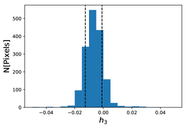
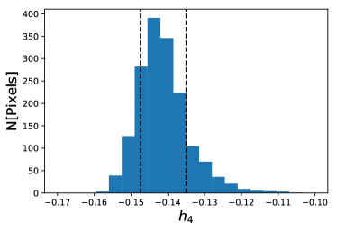
Appendix C Comparison of H ii Region Identification Between KCWI and MUSE
We identify potential H ii regions with H emission maps constructed from the KCWI galaxy mosaics using HIIPhot. H ii regions, for the same galaxies, in the PHANGS Nebular Catalog were identified with HIIPhot and MUSE H maps (Kreckel et al., 2019; Groves et al., 2023). Given the higher resolution of the MUSE imaging, as well as the three-fold brightness increase of H relative to H, we expect our H ii region catalog to be less sensitive to the faintest and smallest H ii regions.
In Figure 20 we show both the distribution of dust-corrected H luminosity, , and radii, for regions identified by HIIPhot using KCWI H maps, “KCWI–H regions”, and MUSE H maps or “MUSE–H regions” within the KCWI mosaic footprint. For KCWI–H regions we measure a median Log) of 37.7 while for MUSE–H regions the median is 37.1. This comparison shows that the KCWI H maps is less sensitive to regions with Log) 37.
We also observe in Figure 20 that regions with radii less than the KCWI angular resolution are missed KCWI–H region sample. This can be seen clearly in Figures 21–27, where we compare the boundaries of the MUSE–H and KCWI–H regions. In these figures, we see that many of the missed regions are small, and unresolved in the KCWI H map. Also owing to the larger number of detections is that many of the larger KCWI–H regions are resolved into smaller structures in the MUSE–H regions.
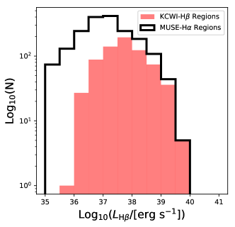
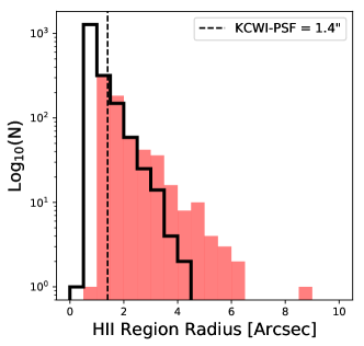
| Name | ||
|---|---|---|
| NGC 628aa NGC 628 was imaged in the least ideal observing conditions. | 10 | 230 |
| NGC 1087 | 173 | 364 |
| NGC 1300 | 60 | 191 |
| NGC 1385 | 133 | 417 |
| NGC 2835 | 87 | 135 |
| NGC 3627 | 163 | 451 |
| NGC 5068 | 62 | 392 |
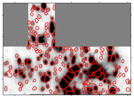
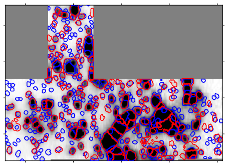
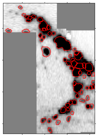
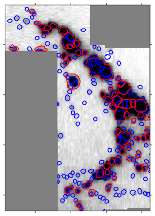
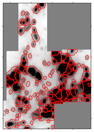
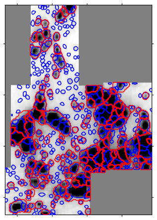
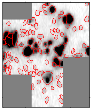
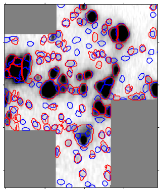
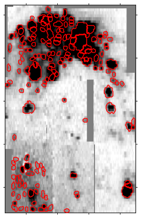
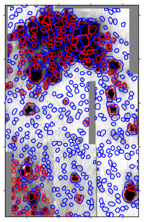
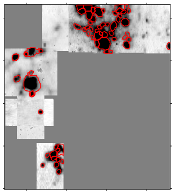
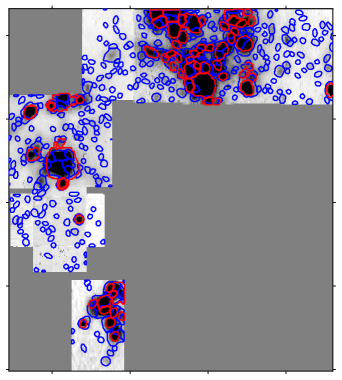
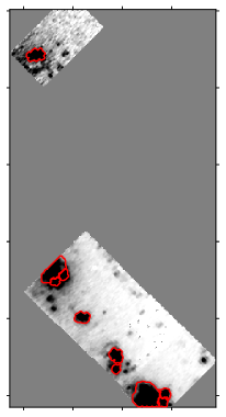
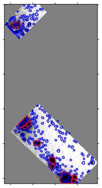
Appendix D Example Gaussian Fits to Auroral Lines
In this section we show example auroral line fits. In Figure 29 we show fits to high S/N auroral lines from an H ii region in NGC 5068. We also include in Figure 29 annotations describing the the standard deviation of the fit residuals, , the S/N for a single emission line (or in the instance of simultaneous double line fits the S/N of the red and purple Gaussian fit: S/Nr and S/Np), the continuum noise, and reduced . In this particular example, the auroral line in these fits are isolated from contaminating sky lines or nearby emission, especially in the case of [O III] Å where the contribution from [Fe II] Å is negligible. To demonstrate fitting [Fe II] alongside [O III] we show a low S/N detection with non-negligible contamination from [Fe II] Å in Figure 30.
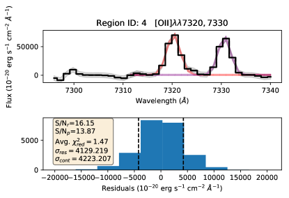
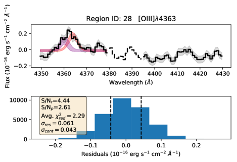
Appendix E Figures of the and H ii Region Property Comparisons
In the section we present the comparisons between H ii region properties that exhibit no significant correlations with .
