Kinematic scheme study of the $O(a^{4})$ Bjorken sum rule and R ratio

Abstract. The Bjorken sum rule and R ratio are constructed to $O(a^{4})$ in the Landau gauge in the three momentum subtraction schemes of Celmaster and Gonsalves where $a$ $=$ $g^{2}/(16\pi^{2})$. We aim to examine the issue of convergence for observables in the various schemes as well as to test ideas on whether using the discrepancy in different scheme values is a viable and more quantum field theoretic alternative to current ways of estimating the theory error on a measureable.

LTH 1352

1 Introduction.

Latterly the development of new methods to evaluate massless Feynman graphs has led to the computation of various important quantities in Quantum Chromodynamics (QCD) to very high loop order. Aside from the recent determination of the five loop QCD $\beta$-function in the modified minimal subtraction ($\overline{\mbox{MS}}$) scheme, [1, 2, 3, 4, 5], that underlies the behaviour of the gauge coupling constant $g$, the extension of the Bjorken sum rule, [6, 7, 8, 9], and the R ratio, [10, 11, 12, 13, 14, 15, 16, 17, 18, 19], to high loop order has led to a greater precision for comparing to experiment and improving estimates of $\alpha_{s}(M_{Z})$ for example. Here $M_{Z}$ is the mass of the $Z$ boson and $\alpha_{s}$ is the strong coupling constant with $\alpha_{s}$ $=$ $g^{2}/(4\pi)$. This is important at present since the improvement in collider data necessarily requires that quantum field theory precision has to develop in parallel. Despite the progress in Feynman integral evaluation in general, the error in measurements is invariably dominated by theory uncertainty. From a theoretical point of view the perturbative expansions at high loop order are always advanced first in the $\overline{\mbox{MS}}$ scheme. This is primarily due to the fact that one only requires the poles with respect to the regularizing parameter to determine the renormalization constants. However, the scheme has a drawback in that it is not a kinematic one. By this we mean that provided the subtraction point where the $\overline{\mbox{MS}}$ renormalization constants are defined is not problematic, such as inadvertently and incorrectly introducing infrared singularities, then it carries no information associated with the kinematics of the subtraction point. Conceptually in an experiment one makes a measurement of say the interaction strength at a specific momentum configuration. The value recorded there can be tied to the value of the coupling constant in the underlying quantum field theory. By the same token one can define, in a parallel sense, the renormalization of the coupling constant at a particular subtraction point. Then a kinematic scheme is constructed through a vertex function by defining the coupling constant renormalization constant in such a way that after renormalization the vertex function is precisely the renormalized coupling constant. In other words the finite part of the vertex function at the subtraction point momentum configuration is fully absorbed into the renormalization constant. This differs from the $\overline{\mbox{MS}}$ scheme where the finite part is ignored in defining the coupling constant renormalization constant.

A set of such schemes was introduced in QCD in the work of Celmaster and Gonsalves, [20, 21]. In those articles three momentum subtraction (MOM) schemes were constructed each based on the three $3$-point vertices of the QCD Lagrangian. They were denoted by MOMg, MOMc and MOMq and based respectively on the triple gluon, ghost-gluon and quark-gluon vertices. More precisely the kinematic configuration considered in [20, 21] was the fully symmetric point where the squared momenta of the three external legs of the respective vertices were equal. In addition in [12, 13] the R ratio was computed in each MOM scheme to ascertain the respective behaviours. While the low loop order studied in [12, 13] was not high enough to come to concrete conclusions there has been a renewed interest in the development and application of MOM schemes to the behaviour of observables. This has been brought about via the development of the Laporta algorithm [22]. That technique opens the way to evaluate two and three loop $3$-point vertex functions which can be achieved once the underlying master Feynman integrals are known. Consequently the three QCD MOM $\beta$-functions were calculated first to three loops in [23] and then more recently to four loops in [24]. The former was an exact computation in the sense that the masters were known analytically. Earlier work on the MOM $\beta$-functions at that order had been numerical [25]. There the masters were determined by applying the Mincer algorithm, [26], to the momentum expansion of each master to high numerical precision before resumming. The remarkable accuracy of [25] was apparent once the analytic result became available. A similar approach was adapted to extract the three loop symmetric point masters again using Mincer, [24]. Exploiting the PSLQ algorithm [27] allowed for the translation of the highly precise numerical values of the masters, derived with Mincer and other methods, to analytic functions whose arguments were the sixth roots of unity, [24]. It is known that such constants have a connection to cyclotomic polynomials, [28]. One consequence of [23] was that the R ratio was determined in the MOM schemes to $O(a^{3})$ in [29], where $a$ $=$ $g^{2}/(16\pi^{2})$, thereby extending [12, 13]. This was an instance where the behaviour of an observable could be compared in kinematic schemes to those in non-kinematic ones such as $\overline{\mbox{MS}}$. Indeed another non-kinematic one was also considered which was the minimal MOM (mMOM) scheme. It was introduced in [30] and is based on the ghost-gluon vertex where the momentum of one of the external ghosts is nullified. In essence it endeavours to preserve Taylor’s observation that the ghost-gluon vertex is finite in the Landau gauge, [31], for other covariant linear gauges. The mMOM renormalization group functions have been determined to high loop order, [30, 32, 33]. For the purely theoretical situation where quarks are massless as well as overlooking resonances and so forth the R ratio behaviour was different in the various schemes.

One concern was that with the predominant use of the $\overline{\mbox{MS}}$ scheme expressions in error analyses there was potentially another source of theory discrepancy lurking in the scheme variations. This is primarily due to the truncation of a series which invariably misses information. To address this scheme issue various methods have been developed and used to significantly improve the truncation uncertainty. There have been several main approaches and we draw attention to the more popular ones where the associated references are not an exhaustive nor definitive list. Rather they are a rough signpost to recent literature. For instance a widely used method to estimate higher order corrections or theoretical uncertainties is to use the conventional scale setting method. In this case the theoretical error at a particular momentum $Q$ is estimated by the maximum and mimimum values of the measureable in the range $[\mbox{\small{$\frac{1}{2}$}}Q,2Q]$ at the highest available loop order of a particular scheme. One drawback of this is that the value at $\mbox{\small{$\frac{1}{2}$}}Q$ may be at a point outside the range of perturbative reliability. By contrast the method known as the Principle of Maximal Conformality (PMC) has been developed in various directions, [34], and widely applied to several observables. It has a more field theoretic origin and has been shown to reduce the scale and scheme uncertainties significantly. For a recent comprehensive review see, for instance, [35]. In the context of this article several current studies are worth noting. For example, the PMC was applied to kinematic schemes in [36] where the role of the covariant gauge parameter, $\alpha$, was included in the analysis. While the $\overline{\mbox{MS}}$ $\beta$-function does not depend on that parameter, [37], this is not the case in MOM schemes as the explicit $\alpha$ dependence for the three MOM $\beta$-functions is available, [20, 21, 23]. Such PMC studies have shown interesting properties. For instance, in [38] a PMC study of the $V$-scheme, [39, 40], shows that it has advantageous properties compared to the $\overline{\mbox{MS}}$ scheme. Other approaches include the Principle of Minimal Sensitivity, [41, 42, 43], effective charges, [44, 45, 46], the Brodsky-Lepage-Mackenzie method, [47] as well as the more recent development of the Principle of Observable Effective Matching, [48]. A comprehensive review of the scale setting problem in QCD can be found, for instance, in [49]. Additionally there are other approaches such as those that extract information about the higher order terms in the perturbative expansion of various quantities. A recent study that employs such a technique can be found in [50] for example. Rather than attempt to fix the scheme or scale to mitigate residual theoretical uncertainties, in this study we attempt to understand and quantify the scheme dependence in high loop calculations to improve our understanding of the parameterization of theory error in these terms, a technique that is applied in [51, 52]. Moreover while our investigation will be at a more theoretical level it is worth noting that the interplay of schemes with error analysis has already been examined in a more phenomenological context. See, for example, [53] for a electroweak sector study as well as, for instance, [54, 55, 56] where the extraction of the top quark mass was considered in the top mass scheme. A more recent study [57] employed renormalization group summed perturbation theory to explore convergence and scale dependence in the mMOM scheme for the R ratio and Higgs boson decay.

While such probes of the higher order behaviour have improved our understanding of experimental results an equally useful way is to determine as far as possible the highest order calculable in the perturbative expansion in a variety of schemes to see if the scheme dependence shows signs of being washed out as the loop order increases. That is the purpose of this article. We will extend the R ratio calculation in the MOM schemes of [20, 21] to the order beyond that computed in [29] which will be to the same order of expansion as the R ratio in the $\overline{\mbox{MS}}$ and mMOM schemes. Therefore we will have a reasonable number of terms in the perturbative series to investigate whether the scheme dependence diminishes. We will carry this out not only for the R ratio but also for the flavour non-singlet Bjorken sum rule [58, 59]. One reason for considering this quantity as well is partly to see if a similar behaviour of scheme independence emerges. To quantify this in our approach in a practical way we will gauge the theory error from each of the schemes at successive loop orders by extracting estimates for $\alpha_{s}(M_{Z})$ using experimental data sets. It should be the case that at higher orders agreement on these ought to improve. We stress, however, that our study in the main will purely be in a theory laboratory. By this we mean quarks will be massless and we will ignore resonances that are inevitably present in experimental data. This is because we want to concentrate and particularly focus on the scheme dependence issue without the complication or distraction of other features. For instance including quark masses in a MOM scheme R ratio evaluation is not straightforward. This is because to have analytic results for the three loop R ratio would require two loop symmetric point $3$-point master integrals as a function of the quark masses in order to renormalize the Lagrangian in a MOM scheme as a function of mass. Such masters are not currently known. Once the scheme issues are understood in this idealized massless setting and the significance of the kinematic schemes quantified then quark mass effects could be included within our framework possibly via a numerical approach. Moreover modelling and including resonance effects for instance has not been tackled yet for MOM schemes as such. It would necessitate the use of a controlled approximation dependent on an appropriate mass scale in each case.

The article is organized as follows. We provide an overview of the perturbative expressions for the Bjorken sum rule and R ratio at high loop order in various renormalization schemes in Section $2$. These then form the foundation for our analysis of the scheme dependence in Section $3$ where for example we examine the convergence properties of an effective coupling constant derived from each observable. The not unrelated issue of assigning an error to such an analysis is discussed in Section $4$ for each of the schemes we consider and we also provide estimates of $\alpha_{s}(M_{Z})$ as a benchmark test. Finally concluding comments are provided in Section $5$.

2 MOM scheme.

Before discussing the construction of the MOM scheme expressions we recall the background to the two quantities of interest. First, the Bjorken sum rule originates from polarized deep inelastic scattering [58, 59] where it measures properties of the distribution of quark spins inside nucleons. In particular the integral over all momentum fractions is defined as

$$\Gamma_{1}^{p-n}(Q^{2})~{}=~{}\int_{0}^{1}\left[g_{1}^{ep}(x,Q^{2})~{}-~{}g_{1}^{en}(x,Q^{2})\right]dx$$ (2.1)

where $Q^{2}$ $=$ $-$ $q^{2}$ and $g_{1}^{ep}$ and $g_{1}^{en}$ are the structure functions associated with the spin of the proton ($p$) and neutron ($n$) respectively. If the parton model point of view was valid in experiments then $\Gamma_{1}^{p-n}(Q^{2})$ would equate exactly to $\mbox{\small{$\frac{1}{6}$}}g_{A}$ where $g_{A}$ is the nucleon axial charge deduced from neutron $\beta$-decay. However due to quantum corrections deriving from QCD and from a wealth of experimental evidence the equality does not hold and theoretically $\Gamma_{1}^{p-n}(Q^{2})$ depends on the strong coupling constant $a$ taking the form

$$\Gamma_{1}^{p-n}(Q^{2})~{}=~{}\frac{g_{A}}{6}C_{{\mbox{\footnotesize{Bjr}}}}(a,\alpha)~{}+~{}\sum_{r=2}^{\infty}\frac{\mu^{p-n}_{2r}(Q^{2})}{(Q^{2})^{r-1}}$$ (2.2)

where Bjr denotes the Bjorken sum rule and the second term represents contributions from twists higher than $2$ reflecting non-perturbative contributions. By constrast $C_{{\mbox{\footnotesize{Bjr}}}}(a,\alpha)$ is perturbatively accessible and is determined from computing the correlation function of the axial vector current in the operator product expansion. In particular the expansion of $C_{{\mbox{\footnotesize{Bjr}}}}(a,\alpha)$ begins with unity. Our focus will be on this contribution and not the non-perturbative piece. We have included the gauge parameter $\alpha$ in the argument of $C_{{\mbox{\footnotesize{Bjr}}}}(a,\alpha)$ since such dependence will in general be present in many schemes although it is absent in the $\overline{\mbox{MS}}$ scheme.

The second quantity of interest is the hadronic R ratio which is related to the correlation function of the electromagnetic current $j_{\mu}$. It is defined by

$$R(s)~{}=~{}12\pi\,\mbox{Im}\,\Pi(-s-i\varepsilon)$$ (2.3)

with $\Pi(Q^{2})$ connected to the correlation function via

$$\Pi_{\mu\nu}(Q^{2})~{}=~{}\frac{i}{Q^{2}}\int\,d^{4}x\,e^{iqx}\langle 0|Tj_{\mu}(x)j_{\nu}(0)|0\rangle$$ (2.4)

where

$$\Pi_{\mu\nu}(q^{2})~{}=~{}-~{}\left[q^{2}\eta_{\mu\nu}-q_{\mu}q_{\nu}\right]\Pi(q^{2})~{}.$$ (2.5)

For practical purposes we remove a common factor by defining

$$R(s)~{}=~{}N_{\!F}\left(\sum_{f}Q_{f}^{2}\right)r(a(s))$$ (2.6)

where $N_{\!F}$ is the dimension of the fundamental representation of the colour group and $Q_{f}$ is the charge of the active quark flavours at energy $s$. We note that when the correlation function contains flavour singlet currents $r(a(s))$ will involve terms involving another function of $Q_{f}$. Our focus here however will be on the non-singlet case. Singlet terms begin at $O(a^{3})$.

Having introduced the background to the Bjorken sum rule and R ratio we now discuss the derivation of the $O(a^{4})$ loop expressions for each in the various kinematic schemes associated with momentum subtraction. To construct the respective MOM scheme results at $O(a^{4})$ we exploit a property of the renormalization group equation. Roughly stated if a quantity is available at Ł loops in one scheme then it can be deduced at the same loop order in another scheme from the relation of the coupling constant in the new scheme to that in the old scheme at $(\mbox{\L}-1)$ loops. To achieve this requires the $\beta$-function at $(\mbox{\L}-1)$ loops in the new scheme. These have been provided recently for the three MOM schemes in [24] in the Landau gauge, defined by $\alpha$ $=$ $0$, where QCD was renormalized to three loops in each of the three MOM schemes extending the one and two loop computations of [20, 21, 23]. Therefore we have used the coupling constant maps recorded in [20, 21, 23, 24] and applied them to the two objects of interest in the Landau gauge. While the two loop maps have been constructed for arbitrary $\alpha$ the three loop MOM $\beta$-function computation was only carried out solely for the Landau gauge, [24]. This is sufficient for our analysis. As the full expressions are long, in order to illustrate the structure of what emerges we record the MOMq expressions both for the Bjorken sum rule and the R ratio in $SU(3)$. An important tool employed in this respect in our calculations throughout was the symbolic manipulation language Form, [60, 61]. In the case of the Bjorken sum rule we have

$$\left.C^{\mbox{\footnotesize{MOMq}}}_{{\mbox{\footnotesize{Bjr}}}}(a,0)\right|_{SU(3)} = 1-4a~{}+~{}[72N_{\!f}-510\psi^{(1)}({\mbox{\small{$\frac{1}{3}$}}})+340\pi^{2}+1269]\frac{a^{2}}{81}$$ (2.7)

$$+~{}[1258848\psi^{(1)}({\mbox{\small{$\frac{1}{3}$}}})N_{\!f}-233280N_{\!f}^{2}-11664\psi^{(3)}({\mbox{\small{$\frac{1}{3}$}}})N_{\!f}+31104\pi^{4}N_{\!f}$$

$$~{}~{}~{}~{}-839232\pi^{2}N_{\!f}+3094848\zeta_{3}N_{\!f}-5598720\zeta_{5}N_{\!f}+6114528N_{\!f}$$

$$~{}~{}~{}~{}-962190\psi^{(1)}({\mbox{\small{$\frac{1}{3}$}}})^{2}+1282920\psi^{(1)}({\mbox{\small{$\frac{1}{3}$}}})\pi^{2}-8916966\psi^{(1)}({\mbox{\small{$\frac{1}{3}$}}})$$

$$~{}~{}~{}~{}-13635\psi^{(3)}({\mbox{\small{$\frac{1}{3}$}}})-391280\pi^{4}+5944644\pi^{2}-21121074\zeta_{3}$$

$$~{}~{}~{}~{}+92378880\zeta_{5}-52764048]\frac{a^{3}}{52488}$$

$$+~{}[20623196160H_{5}N_{\!f}+187812172800H_{5}+2267136H_{6}$$

$$~{}~{}~{}~{}+9405849600N_{\!f}^{3}-2821754880\psi^{(1)}({\mbox{\small{$\frac{1}{3}$}}})^{2}N_{\!f}^{2}$$

$$~{}~{}~{}~{}+3762339840\psi^{(1)}({\mbox{\small{$\frac{1}{3}$}}})\pi^{2}N_{\!f}^{2}-15049359360\psi^{(1)}({\mbox{\small{$\frac{1}{3}$}}})\zeta_{3}N_{\!f}^{2}$$

$$~{}~{}~{}~{}-169462056960\psi^{(1)}({\mbox{\small{$\frac{1}{3}$}}})N_{\!f}^{2}+1516838400\psi^{(3)}({\mbox{\small{$\frac{1}{3}$}}})N_{\!f}^{2}$$

$$~{}~{}~{}~{}-5299015680\pi^{4}N_{\!f}^{2}+10032906240\pi^{2}\zeta_{3}N_{\!f}^{2}$$

$$~{}~{}~{}~{}+112974704640\pi^{2}N_{\!f}^{2}-135444234240\zeta_{3}^{2}N_{\!f}^{2}$$

$$~{}~{}~{}~{}+750691307520\zeta_{3}N_{\!f}^{2}-790091366400\zeta_{5}N_{\!f}^{2}$$

$$~{}~{}~{}~{}-366253332480N_{\!f}^{2}+40828354560\psi^{(1)}({\mbox{\small{$\frac{1}{3}$}}})^{3}N_{\!f}$$

$$~{}~{}~{}~{}-81656709120\psi^{(1)}({\mbox{\small{$\frac{1}{3}$}}})^{2}\pi^{2}N_{\!f}+155496983040\psi^{(1)}({\mbox{\small{$\frac{1}{3}$}}})^{2}N_{\!f}$$

$$~{}~{}~{}~{}-4996857600\psi^{(1)}({\mbox{\small{$\frac{1}{3}$}}})\psi^{(3)}({\mbox{\small{$\frac{1}{3}$}}})N_{\!f}+67762759680\psi^{(1)}({\mbox{\small{$\frac{1}{3}$}}})\pi^{4}N_{\!f}$$

$$~{}~{}~{}~{}-207329310720\psi^{(1)}({\mbox{\small{$\frac{1}{3}$}}})\pi^{2}N_{\!f}+1134305399808\psi^{(1)}({\mbox{\small{$\frac{1}{3}$}}})\zeta_{3}N_{\!f}$$

$$~{}~{}~{}~{}-1598994432000\psi^{(1)}({\mbox{\small{$\frac{1}{3}$}}})\zeta_{5}N_{\!f}+6622411146624\psi^{(1)}({\mbox{\small{$\frac{1}{3}$}}})N_{\!f}$$

$$~{}~{}~{}~{}+3331238400\psi^{(3)}({\mbox{\small{$\frac{1}{3}$}}})\pi^{2}N_{\!f}-147525507360\psi^{(3)}({\mbox{\small{$\frac{1}{3}$}}})N_{\!f}$$

$$~{}~{}~{}~{}+452620224\psi^{(5)}({\mbox{\small{$\frac{1}{3}$}}})N_{\!f}-41901705216\pi^{6}N_{\!f}+462511123200\pi^{4}N_{\!f}$$

$$~{}~{}~{}~{}-756203599872\pi^{2}\zeta_{3}N_{\!f}+1065996288000\pi^{2}\zeta_{5}N_{\!f}$$

$$~{}~{}~{}~{}-4414940764416\pi^{2}N_{\!f}+4469659729920\zeta_{3}^{2}N_{\!f}$$

$$~{}~{}~{}~{}-12921382559232\zeta_{3}N_{\!f}+7683712081920\zeta_{5}N_{\!f}$$

$$~{}~{}~{}~{}+8295959347200\zeta_{7}N_{\!f}-318923619840N_{\!f}-453980630880\psi^{(1)}({\mbox{\small{$\frac{1}{3}$}}})^{3}$$

$$~{}~{}~{}~{}+907961261760\psi^{(1)}({\mbox{\small{$\frac{1}{3}$}}})^{2}\pi^{2}-2555163443700\psi^{(1)}({\mbox{\small{$\frac{1}{3}$}}})^{2}$$

$$~{}~{}~{}~{}-11132857680\psi^{(1)}({\mbox{\small{$\frac{1}{3}$}}})\psi^{(3)}({\mbox{\small{$\frac{1}{3}$}}})-575619887360\psi^{(1)}({\mbox{\small{$\frac{1}{3}$}}})\pi^{4}$$

$$~{}~{}~{}~{}+3406884591600\psi^{(1)}({\mbox{\small{$\frac{1}{3}$}}})\pi^{2}+1202060938176\psi^{(1)}({\mbox{\small{$\frac{1}{3}$}}})\zeta_{3}$$

$$~{}~{}~{}~{}+26383408128000\psi^{(1)}({\mbox{\small{$\frac{1}{3}$}}})\zeta_{5}-41716811068632\psi^{(1)}({\mbox{\small{$\frac{1}{3}$}}})$$

$$~{}~{}~{}~{}+7421905120\psi^{(3)}({\mbox{\small{$\frac{1}{3}$}}})\pi^{2}+1041696774405\psi^{(3)}({\mbox{\small{$\frac{1}{3}$}}})$$

$$~{}~{}~{}~{}-2561413512\psi^{(5)}({\mbox{\small{$\frac{1}{3}$}}})+233115257088\pi^{6}-3913486262280\pi^{4}$$

$$~{}~{}~{}~{}-801373958784\pi^{2}\zeta_{3}-17588938752000\pi^{2}\zeta_{5}+27811207379088\pi^{2}$$

$$~{}~{}~{}~{}-36874692771840\zeta_{3}^{2}+97876178446536\zeta_{3}-48763797737760\zeta_{5}$$

$$~{}~{}~{}~{}-136883329228800\zeta_{7}+44612309619360]\frac{a^{4}}{3174474240}$$

$$~{}~{}~{}~{}+~{}O(a^{5})$$

where the variable $a$ here is in the MOMq scheme. We use the convention that when an object is labelled by a scheme then the variables of the expression are in that scheme. We follow the notation of [24] which results in a variety of numbers such as the Riemann zeta series $\zeta_{n}$ and the odd derivatives of the Euler $\psi$-function, $\psi(z)$, up to the fifth order. The first and third order derivatives appeared first in the one and two loop expressions respectively. However comparing the form of the two loop term of the coupling constant mapping for the MOM schemes with the same terms given in [24] it is clear that the latter expressions are much simpler. This was highlighted in [24] and is due to a relation between harmonic polylogarithms that were present in the two loop symmetric point master integrals computed directly in [62, 63, 64, 65, 66]. In [24, 67] an indirect method was chosen to compute the masters. This involved using the Mincer algorithm, [26], to evaluate the symmetric point masters by using a Taylor series expansion in the limit as one of the external momenta approaches zero, [25]. The resulting expression was computed to very high numerical accuracy and then reconstructed analytically using the PSLQ algorithm, [27]. At two loops the basis choice used for the PSLQ fit included rationals, $\pi$, $\zeta_{2}$, $\zeta_{3}$, $\zeta_{4}$, $\zeta_{5}$, $\psi^{(1)}({\mbox{\small{$\frac{1}{3}$}}})$ and $\psi^{(3)}({\mbox{\small{$\frac{1}{3}$}}})$ and combinations. The absence of harmonic polylogarithms that appeared in previous work, [23], is because it is now known that they were not independent of the basis choice [24]. One specific relation was recorded in [68] which we recall is

$$s_{2}\left(\mbox{\small{$\frac{\pi}{6}$}}\right) = \frac{1}{11664}\left[324\sqrt{3}\ln(3)\pi-27\sqrt{3}\ln^{2}(3)\pi+29\sqrt{3}\pi^{3}-1944\psi^{(1)}({\mbox{\small{$\frac{1}{3}$}}})\right.$$ (2.8)

$$\left.~{}~{}~{}~{}~{}~{}~{}~{}~{}+23328s_{2}\left(\mbox{\small{$\frac{\pi}{2}$}}\right)+19440s_{3}\left(\mbox{\small{$\frac{\pi}{6}$}}\right)-15552s_{3}\left(\mbox{\small{$\frac{\pi}{2}$}}\right)+1296\pi^{2}\right]$$

and holds numerically where

$$s_{n}(z)~{}=~{}\frac{1}{\sqrt{3}}\mbox{Im}\,\left[\mbox{Li}_{n}\left(\frac{e^{iz}}{\sqrt{3}}\right)\right]$$ (2.9)

and $\mbox{Li}_{n}(z)$ is the polylogarithm function. The linear combination of $s_{2}\left(\mbox{\small{$\frac{\pi}{2}$}}\right)$, $s_{2}\left(\mbox{\small{$\frac{\pi}{6}$}}\right)$, $s_{3}\left(\mbox{\small{$\frac{\pi}{2}$}}\right)$ and $s_{3}\left(\mbox{\small{$\frac{\pi}{6}$}}\right)$ that appear in the two loop masters of [62, 63, 64, 65, 66] together with the terms with an odd power of $\pi$ is the same as that which occurs in (2.8). At $O(a^{4})$ the quantities $H_{5}$ and $H_{6}$ appear and the lengthy definitions for them are given explicitly in terms of both generalized and harmonic polylogarithms in the info.pdf file accessible from the Supplemental Material associated with [24]. The three loop master integrals that underpin [24] are recorded in [67]. We note that electronic versions of (2.7) as well as similar expressions in the other Landau gauge MOM schemes are available for an arbitrary colour group in the data file of the associated arXiv version of this article. It also contains the parallel data for the R ratio.

While the expressions for the other two kinematic schemes have a similar structure what is perhaps more instructive is to record the numerical expressions for all the schemes we will consider here. For instance for the $SU(3)$ group we have

$$\left.C^{\overline{\mbox{\footnotesize{MS}}}}_{{\mbox{\footnotesize{Bjr}}}}(a,0)\right|_{SU(3)} = 1-4.000000a+[5.333333N_{\!f}-73.333333]a^{2}$$

$$+~{}[-11.358025N_{\!f}^{2}+486.866536N_{\!f}-2652.1544368]a^{3}$$

$$+~{}[26.556927N_{\!f}^{3}-1970.551732N_{\!f}^{2}+31588.209324N_{\!f}$$

$$~{}~{}~{}~{}-122738.570412]a^{4}~{}+~{}O(a^{5})$$

$$\left.C^{\mbox{\footnotesize{MOMg}}}_{{\mbox{\footnotesize{Bjr}}}}(a,0)\right|_{SU(3)} = 1-4.000000a+[-8.333892N_{\!f}+32.636622]a^{2}$$

$$+~{}[-37.559047N_{\!f}^{2}+343.123637N_{\!f}-539.554265]a^{3}$$

$$+~{}[-190.378849N_{\!f}^{3}+2382.689181N_{\!f}^{2}-8789.557343N_{\!f}$$

$$~{}~{}~{}~{}+3685.269188]a^{4}~{}+~{}O(a^{5})$$

$$\left.C^{\mbox{\footnotesize{MOMq}}}_{{\mbox{\footnotesize{Bjr}}}}(a,0)\right|_{SU(3)} = 1-4.000000a+[0.888889N_{\!f}-6.470235]a^{2}$$

$$+~{}[-4.444444N_{\!f}^{2}+110.326436N_{\!f}-547.208073]a^{3}$$

$$+~{}[2.962963N_{\!f}^{3}-260.408043N_{\!f}^{2}+4464.055445N_{\!f}-19390.815675]a^{4}$$

$$+~{}O(a^{5})$$

$$\left.C^{\mbox{\footnotesize{MOMc}}}_{{\mbox{\footnotesize{Bjr}}}}(a,0)\right|_{SU(3)} = 1-4.000000a+[0.888889N_{\!f}+0.8597681]a^{2}$$

$$+~{}[-4.444444N_{\!f}^{2}+113.578619N_{\!f}-116.288597]a^{3}$$

$$+~{}[2.962963N_{\!f}^{3}-195.703375N_{\!f}^{2}+2213.334884N_{\!f}-10426.816777]a^{4}$$

$$+~{}O(a^{5})$$

$$\left.C^{\mbox{\footnotesize{mMOM}}}_{{\mbox{\footnotesize{Bjr}}}}(a,0)\right|_{SU(3)} = 1-4.000000a+[0.888889N_{\!f}-17.000000]a^{2}$$ (2.10)

$$+~{}[-4.444444N_{\!f}^{2}+134.233344N_{\!f}-271.420979]a^{3}$$

$$+~{}[2.962963N_{\!f}^{3}-278.134393N_{\!f}^{2}+4556.133051N_{\!f}-17123.525160]a^{4}$$

$$+~{}O(a^{5})$$

in the Landau gauge where the $O(a^{4})$ $\overline{\mbox{MS}}$ result was provided in [9] and that for the minimal momentum (mMOM) scheme was given in [69]. Clearly the $O(a)$ term is scheme independent. The higher order terms show no commonality. For instance the sign of the leading $N_{\!f}$ term at each order varies from scheme to scheme. Moreover the $O(a^{4})$ $N_{\!f}$ independent term ranges over two orders of magnitude from the $\overline{\mbox{MS}}$ scheme to the MOMg one. This of course does not mean that $C^{\overline{\mbox{\footnotesize{MS}}}}_{{\mbox{\footnotesize{Bjr}}}}(a,0)$ is not as accurate as the expression in the latter scheme. The reason for this is that aside from the fact that the expansion variables are different in each scheme, the coupling constant is itself a function that depends on the underlying momentum scale. Explicitly including the momentum dependence of the running coupling in each scheme balances out the apparent disparity in the coefficients we mentioned.

Having focused on the derivation of the Bjorken sum rule in kinematic schemes we have repeated the exercise for the R ratio. So for instance the MOMq scheme version is

$$\left.r^{\mbox{\footnotesize{MOMq}}}(a)\right|_{SU(3)} = 1+4a+[864\zeta_{3}N_{\!f}-828N_{\!f}+510\psi^{(1)}({\mbox{\small{$\frac{1}{3}$}}})-340\pi^{2}-14256\zeta_{3}+12501]\frac{a^{2}}{81}$$ (2.11)

$$+\left[\left[855360-1866240\zeta_{3}\right]\eta-31104\pi^{2}N_{\!f}^{2}-1119744\zeta_{3}N_{\!f}^{2}+1679616N_{\!f}^{2}\right.$$

$$\left.~{}~{}~{}~{}+1762560\psi^{(1)}({\mbox{\small{$\frac{1}{3}$}}})\zeta_{3}N_{\!f}-2801088\psi^{(1)}({\mbox{\small{$\frac{1}{3}$}}})N_{\!f}+11664\psi^{(3)}({\mbox{\small{$\frac{1}{3}$}}})N_{\!f}\right.$$

$$\left.~{}~{}~{}~{}-31104\pi^{4}N_{\!f}-1175040\pi^{2}\zeta_{3}N_{\!f}+2893824\pi^{2}N_{\!f}+53047872\zeta_{3}N_{\!f}\right.$$

$$\left.~{}~{}~{}~{}-9331200\zeta_{5}N_{\!f}-59723568N_{\!f}+962190\psi^{(1)}({\mbox{\small{$\frac{1}{3}$}}})^{2}-1282920\psi^{(1)}({\mbox{\small{$\frac{1}{3}$}}})\pi^{2}\right.$$

$$\left.~{}~{}~{}~{}-29082240\psi^{(1)}({\mbox{\small{$\frac{1}{3}$}}})\zeta_{3}+37007766\psi^{(1)}({\mbox{\small{$\frac{1}{3}$}}})+13635\psi^{(3)}({\mbox{\small{$\frac{1}{3}$}}})+391280\pi^{4}\right.$$

$$\left.~{}~{}~{}~{}+19388160\pi^{2}\zeta_{3}-33139908\pi^{2}-510524046\zeta_{3}+153964800\zeta_{5}\right.$$

$$\left.~{}~{}~{}~{}+455543352\right]\frac{a^{3}}{52488}$$

$$+\left[\left[225740390400\zeta_{3}^{2}N_{\!f}+357422284800\zeta_{3}N_{\!f}-564350976000\zeta_{5}N_{\!f}\right.\right.$$

$$\left.\left.~{}~{}~{}~{}-294716620800N_{\!f}-532998144000\psi^{(1)}({\mbox{\small{$\frac{1}{3}$}}})\zeta_{3}\right.\right.$$

$$\left.\left.~{}~{}~{}~{}+244290816000\psi^{(1)}({\mbox{\small{$\frac{1}{3}$}}})+355332096000\pi^{2}\zeta_{3}-162860544000\pi^{2}\right.\right.$$

$$\left.\left.~{}~{}~{}~{}-3724716441600\zeta_{3}^{2}-7976160460800\zeta_{3}+10628610048000\zeta_{5}\right.\right.$$

$$\left.\left.~{}~{}~{}~{}+4722912230400\right]\eta\right.$$

$$\left.~{}~{}~{}~{}-20623196160H_{5}N_{\!f}-187812172800H_{5}-2267136H_{6}\right.$$

$$\left.~{}~{}~{}~{}-15049359360\pi^{2}\zeta_{3}N_{\!f}^{3}+14422302720\pi^{2}N_{\!f}^{3}+158018273280\zeta_{3}N_{\!f}^{3}\right.$$

$$\left.~{}~{}~{}~{}+225740390400\zeta_{5}N_{\!f}^{3}-378115153920N_{\!f}^{3}+2821754880\psi^{(1)}({\mbox{\small{$\frac{1}{3}$}}})^{2}N_{\!f}^{2}\right.$$

$$\left.~{}~{}~{}~{}-12645642240\psi^{(1)}({\mbox{\small{$\frac{1}{3}$}}})\pi^{2}N_{\!f}^{2}-663425925120\psi^{(1)}({\mbox{\small{$\frac{1}{3}$}}})\zeta_{3}N_{\!f}^{2}\right.$$

$$\left.~{}~{}~{}~{}+896377466880\psi^{(1)}({\mbox{\small{$\frac{1}{3}$}}})N_{\!f}^{2}+3762339840\psi^{(3)}({\mbox{\small{$\frac{1}{3}$}}})\zeta_{3}N_{\!f}^{2}\right.$$

$$\left.~{}~{}~{}~{}-4808885760\psi^{(3)}({\mbox{\small{$\frac{1}{3}$}}})N_{\!f}^{2}-10032906240\pi^{4}\zeta_{3}N_{\!f}^{2}+20000010240\pi^{4}N_{\!f}^{2}\right.$$

$$\left.~{}~{}~{}~{}+1187227238400\pi^{2}\zeta_{3}N_{\!f}^{2}-1380621957120\pi^{2}N_{\!f}^{2}\right.$$

$$\left.~{}~{}~{}~{}+902961561600\zeta_{3}^{2}N_{\!f}^{2}-12819963985920\zeta_{3}N_{\!f}^{2}\right.$$

$$\left.~{}~{}~{}~{}-9706836787200\zeta_{5}N_{\!f}^{2}+22470692267520N_{\!f}^{2}\right.$$

$$\left.~{}~{}~{}~{}-40828354560\psi^{(1)}({\mbox{\small{$\frac{1}{3}$}}})^{3}N_{\!f}+81656709120\psi^{(1)}({\mbox{\small{$\frac{1}{3}$}}})^{2}\pi^{2}N_{\!f}\right.$$

$$\left.~{}~{}~{}~{}+394261862400\psi^{(1)}({\mbox{\small{$\frac{1}{3}$}}})^{2}\zeta_{3}N_{\!f}-500476112640\psi^{(1)}({\mbox{\small{$\frac{1}{3}$}}})^{2}N_{\!f}\right.$$

$$\left.~{}~{}~{}~{}+4996857600\psi^{(1)}({\mbox{\small{$\frac{1}{3}$}}})\psi^{(3)}({\mbox{\small{$\frac{1}{3}$}}})N_{\!f}-67762759680\psi^{(1)}({\mbox{\small{$\frac{1}{3}$}}})\pi^{4}N_{\!f}\right.$$

$$\left.~{}~{}~{}~{}-525682483200\psi^{(1)}({\mbox{\small{$\frac{1}{3}$}}})\pi^{2}\zeta_{3}N_{\!f}+960450462720\psi^{(1)}({\mbox{\small{$\frac{1}{3}$}}})\pi^{2}N_{\!f}\right.$$

$$\left.~{}~{}~{}~{}+24529502979072\psi^{(1)}({\mbox{\small{$\frac{1}{3}$}}})\zeta_{3}N_{\!f}-2664990720000\psi^{(1)}({\mbox{\small{$\frac{1}{3}$}}})\zeta_{5}N_{\!f}\right.$$

$$\left.~{}~{}~{}~{}-30896934171264\psi^{(1)}({\mbox{\small{$\frac{1}{3}$}}})N_{\!f}-3331238400\psi^{(3)}({\mbox{\small{$\frac{1}{3}$}}})\pi^{2}N_{\!f}\right.$$

$$\left.~{}~{}~{}~{}-57680501760\psi^{(3)}({\mbox{\small{$\frac{1}{3}$}}})\zeta_{3}N_{\!f}+203639456160\psi^{(3)}({\mbox{\small{$\frac{1}{3}$}}})N_{\!f}\right.$$

$$\left.~{}~{}~{}~{}-452620224\psi^{(5)}({\mbox{\small{$\frac{1}{3}$}}})N_{\!f}+41901705216\pi^{6}N_{\!f}+329042165760\pi^{4}\zeta_{3}N_{\!f}\right.$$

$$\left.~{}~{}~{}~{}-960905030400\pi^{4}N_{\!f}-28644566243328\pi^{2}\zeta_{3}N_{\!f}\right.$$

$$\left.~{}~{}~{}~{}+1776660480000\pi^{2}\zeta_{5}N_{\!f}+33903941250816\pi^{2}N_{\!f}\right.$$

$$\left.~{}~{}~{}~{}-46905874606080\zeta_{3}^{2}N_{\!f}+280279032268032\zeta_{3}N_{\!f}\right.$$

$$\left.~{}~{}~{}~{}+124706756321280\zeta_{5}N_{\!f}+7505867980800\zeta_{7}N_{\!f}\right.$$

$$\left.~{}~{}~{}~{}-389487227794560N_{\!f}+453980630880\psi^{(1)}({\mbox{\small{$\frac{1}{3}$}}})^{3}\right.$$

$$\left.~{}~{}~{}~{}-907961261760\psi^{(1)}({\mbox{\small{$\frac{1}{3}$}}})^{2}\pi^{2}-6505320729600\psi^{(1)}({\mbox{\small{$\frac{1}{3}$}}})^{2}\zeta_{3}\right.$$

$$\left.~{}~{}~{}~{}+8838711875700\psi^{(1)}({\mbox{\small{$\frac{1}{3}$}}})^{2}+11132857680\psi^{(1)}({\mbox{\small{$\frac{1}{3}$}}})\psi^{(3)}({\mbox{\small{$\frac{1}{3}$}}})\right.$$

$$\left.~{}~{}~{}~{}+575619887360\psi^{(1)}({\mbox{\small{$\frac{1}{3}$}}})\pi^{4}+8673760972800\psi^{(1)}({\mbox{\small{$\frac{1}{3}$}}})\pi^{2}\zeta_{3}\right.$$

$$\left.~{}~{}~{}~{}-14203428246000\psi^{(1)}({\mbox{\small{$\frac{1}{3}$}}})\pi^{2}-214276142356416\psi^{(1)}({\mbox{\small{$\frac{1}{3}$}}})\zeta_{3}\right.$$

$$\left.~{}~{}~{}~{}+43972346880000\psi^{(1)}({\mbox{\small{$\frac{1}{3}$}}})\zeta_{5}+215899216511832\psi^{(1)}({\mbox{\small{$\frac{1}{3}$}}})\right.$$

$$\left.~{}~{}~{}~{}-7421905120\psi^{(3)}({\mbox{\small{$\frac{1}{3}$}}})\pi^{2}-72568742400\psi^{(3)}({\mbox{\small{$\frac{1}{3}$}}})\zeta_{3}\right.$$

$$\left.~{}~{}~{}~{}-971601966405\psi^{(3)}({\mbox{\small{$\frac{1}{3}$}}})+2561413512\psi^{(5)}({\mbox{\small{$\frac{1}{3}$}}})-233115257088\pi^{6}\right.$$

$$\left.~{}~{}~{}~{}-2697737011200\pi^{4}\zeta_{3}+8131574351880\pi^{4}+210454364985984\pi^{2}\zeta_{3}\right.$$

$$\left.~{}~{}~{}~{}-29314897920000\pi^{2}\zeta_{5}-215086534781328\pi^{2}+528115645854720\zeta_{3}^{2}\right.$$

$$\left.~{}~{}~{}~{}-1807448276772936\zeta_{3}-436869622959840\zeta_{5}-123846821683200\zeta_{7}\right.$$

$$\left.~{}~{}~{}~{}+2018890127348640\right]\frac{a^{4}}{3174474240}~{}+~{}O(a^{5})$$

for $SU(3)$, also in the Landau gauge, which includes a parameter $\eta$. It is defined to be

$$\eta~{}=~{}\frac{\sum_{f}Q_{f}^{2}}{\left[\sum_{f}Q_{f}\right]^{2}}$$ (2.12)

and is associated with $O(a^{3})$ graphs that contribute to the flavour singlet value of the R ratio. Similar to the Bjorken case we will set $\eta$ $=$ $0$ throughout and concentrate on the non-singlet scenario. Moreover, we have checked that all the MOM scheme $O(a^{3})$ R ratio expressions given in [29] agree with the analytic $O(a^{3})$ expressions derived using the coupling constant mappings provided in [24] after taking (2.8) into account. For completeness we record the $O(a^{4})$ numerical expressions for the R ratio in each scheme. We have

$$\left.r^{\overline{\mbox{\footnotesize{MS}}}}(a)\right|_{SU(3)} = 1+4.000000a+[-1.844726N_{\!f}+31.771318]a^{2}$$

$$+~{}[-26.443505\eta-0.331415N_{\!f}^{2}-76.808579N_{\!f}-424.763877]a^{3}$$

$$+~{}[49.056846\eta N_{\!f}-1521.214892\eta+5.508123N_{\!f}^{3}-204.143191N_{\!f}^{2}$$

$$~{}~{}~{}~{}+~{}4806.339848N_{\!f}-40091.676394]a^{4}~{}+~{}O(a^{5})$$

$$\left.r^{\mbox{\footnotesize{MOMg}}}(a)\right|_{SU(3)} = 1+4.000000a+[11.822499N_{\!f}-74.198637]a^{2}$$

$$+~{}[-26.443505\eta+49.709397N_{\!f}^{2}-401.928163N_{\!f}-335.201612]a^{3}$$

$$+~{}[-222.000165\eta N_{\!f}+580.4478702\eta+252.625523N_{\!f}^{3}-2960.042900N_{\!f}^{2}$$

$$~{}~{}~{}~{}+~{}7418.803963N_{\!f}+12015.778615]a^{4}~{}+~{}O(a^{5})$$

$$\left.r^{\mbox{\footnotesize{MOMq}}}(a)\right|_{SU(3)} = 1+4.000000a+[2.599718N_{\!f}-35.091780]a^{2}$$

$$+~{}[-26.443505\eta+0.507465N_{\!f}^{2}+90.741952N_{\!f}-1140.227696]a^{3}$$

$$+~{}[-39.088169\eta N_{\!f}-195.143901\eta+3.058056N_{\!f}^{3}-183.223433N_{\!f}^{2}$$

$$~{}~{}~{}~{}+~{}3501.125982N_{\!f}-7958.138070]a^{4}~{}+~{}O(a^{5})$$

$$\left.r^{\mbox{\footnotesize{MOMc}}}(a)\right|_{SU(3)} = 1+4.000000a+[2.599718N_{\!f}-42.421783]a^{2}$$

$$+~{}[-26.443505\eta+0.507465N_{\!f}^{2}+74.704019N_{\!f}-1418.822322]a^{3}$$

$$+~{}[-39.088169\eta N_{\!f}-49.770672\eta+3.058056N_{\!f}^{3}-237.639896N_{\!f}^{2}$$

$$~{}~{}~{}~{}+~{}4083.180193N_{\!f}+677.129492]a^{4}~{}+~{}O(a^{5})$$

$$\left.r^{\mbox{\footnotesize{mMOM}}}(a)\right|_{SU(3)} = 1+4.000000a+[2.599718N_{\!f}-24.562015]a^{2}$$ (2.13)

$$+~{}[-26.443505\eta+0.507465N_{\!f}^{2}+85.202150N_{\!f}-1634.833914]a^{3}$$

$$+~{}[-39.088169\eta N_{\!f}-403.976819\eta+3.058056N_{\!f}^{3}-230.126428N_{\!f}^{2}$$

$$~{}~{}~{}~{}+~{}4880.206237N_{\!f}-17400.630113]a^{4}~{}+~{}O(a^{5})~{}.$$

Similar comments to the different scheme expressions of the Bjorken case apply to the R ratio in that there is a large disparity in the numerical values. For instance not only does the size of the coefficients of the $O(a^{4})$ $N_{\!f}$ $=$ $0$ terms have a wide spread but they can have either sign.

3 Analysis.

Our analysis will involve the Bjorken sum rule and the R ratio evaluated in the mMOM, $\overline{\mbox{MS}}$ and the three MOM schemes of [20, 21], that we will collectively denote by MOMi, to provide a comparison of measureable perturbative series considered in different renormalization schemes. As noted the numerical values in (2.10) and (2.13) cannot be directly compared as they are written in terms of the coupling constants for different schemes. Therefore we must have a standard which we use to relate the coupling constants to one another. For example, one could choose to insert the coupling constant conversion functions without truncation to get the series in one scheme in terms of the coupling constant of another. However, as this only makes a connection with the value of an abstract formal quantity, we will instead choose to compare the series at set energy levels by substituting the explicit form of the coupling constant in terms of the unphysical renormalization momentum.

The expression for the coupling constant at a particular energy level can be found by solving the renormalization group equations perturbatively. Denoting the expression for the coupling constant to the Ł-th loop level these expressions are given by

$$a_{1}^{\cal S}(Q,\Lambda^{\cal S}) = \frac{1}{b_{0}^{\cal S}L^{\cal S}},$$

$$a_{2}^{\cal S}(Q,\Lambda^{\cal S}) = \frac{1}{b_{0}^{\cal S}L^{\cal S}}\left[1-\frac{b_{1}^{\cal S}\ln(L^{\cal S})}{{b_{0}^{\cal S}}^{2}L^{\cal S}}\right],$$

$$a_{3}^{\cal S}(Q,\Lambda^{\cal S}) = \frac{1}{b_{0}^{\cal S}L^{\cal S}}\left[1-\frac{b_{1}^{\cal S}\ln(L^{\cal S})}{{b_{0}^{\cal S}}^{2}L^{\cal S}}+\left[{b_{1}^{\cal S}}^{2}\left[\ln^{2}(L^{\cal S})-\ln(L^{\cal S})-1\right]+b_{0}^{\cal S}b_{2}^{\cal S}\right]\frac{1}{{b_{0}^{\cal S}}^{4}{L^{\cal S}}^{2}}\right],$$

$$a_{4}^{\cal S}(Q,\Lambda^{\cal S}) = \frac{1}{b_{0}^{\cal S}L^{\cal S}}\left[1-\frac{b_{1}^{\cal S}\ln(L^{\cal S})}{{b_{0}^{\cal S}}^{2}L^{\cal S}}+\left[{b_{1}^{\cal S}}^{2}\left[\ln^{2}(L^{\cal S})-\ln(L^{\cal S})-1\right]+b_{0}^{\cal S}b_{2}^{\cal S}\right]\frac{1}{{b_{0}^{\cal S}}^{4}{L^{\cal S}}^{2}}\right.$$

$$\left.~{}~{}~{}~{}~{}~{}~{}~{}~{}-\left[{b_{1}^{\cal S}}^{3}\left[\ln^{3}(L^{\cal S})-\frac{5}{2}\ln^{2}(L^{\cal S})-2\ln(L^{\cal S})+\frac{1}{2}\right]+3b_{0}^{\cal S}b_{1}^{\cal S}b_{2}^{\cal S}\ln(L^{\cal S})\right.\right.$$

$$\left.\left.~{}~{}~{}~{}~{}~{}~{}~{}~{}~{}~{}~{}~{}-\frac{1}{2}{b_{0}^{\cal S}}^{2}b_{3}^{\cal S}\right]\frac{1}{{b_{0}^{\cal S}}^{6}{L^{\cal S}}^{3}}\right],$$

$$a_{5}^{\cal S}(Q,\Lambda^{\cal S}) = \frac{1}{b_{0}^{\cal S}L^{\cal S}}\left[1-\frac{b_{1}^{\cal S}\ln(L^{\cal S})}{{b_{0}^{\cal S}}^{2}L^{\cal S}}+\left[{b_{1}^{\cal S}}^{2}\left[\ln^{2}(L^{\cal S})-\ln(L^{\cal S})-1\right]+b_{0}^{\cal S}b_{2}^{\cal S}\right]\frac{1}{{b_{0}^{\cal S}}^{4}{L^{\cal S}}^{2}}\right.$$ (3.1)

$$\left.~{}~{}~{}~{}~{}~{}~{}~{}~{}-\left[{b_{1}^{\cal S}}^{3}\left[\ln^{3}(L^{\cal S})-\frac{5}{2}\ln^{2}(L^{\cal S})-2\ln(L^{\cal S})+\frac{1}{2}\right]+3{b_{0}^{\cal S}}{b_{1}^{\cal S}}{b_{2}^{\cal S}}\ln(L^{\cal S})\right.\right.$$

$$\left.\left.~{}~{}~{}~{}~{}~{}~{}~{}~{}~{}~{}~{}~{}-\frac{1}{2}{b_{0}^{\cal S}}^{2}b_{3}^{\cal S}\right]\frac{1}{{b_{0}^{\cal S}}^{6}{L^{\cal S}}^{3}}\right.$$

$$\left.~{}~{}~{}~{}~{}~{}~{}~{}~{}+\left[18{b_{0}^{\cal S}}{b_{2}^{\cal S}}{b_{1}^{\cal S}}^{2}\left[2\ln^{2}(L^{\cal S})-\ln(L^{\cal S})-1\right]+2{b_{0}^{\cal S}}^{2}\left[5{{b_{2}^{\cal S}}}^{2}+{b_{0}^{\cal S}}{b_{4}^{\cal S}}\right]\right.\right.$$

$$\left.\left.~{}~{}~{}~{}~{}~{}~{}~{}~{}~{}~{}~{}~{}+{b_{1}^{\cal S}}^{4}\left[6\ln^{4}(L^{\cal S})-26\ln^{3}(L^{\cal S})-9\ln^{2}(L^{\cal S})+24\ln(L^{\cal S})+7\right]\right.\right.$$

$$\left.\left.~{}~{}~{}~{}~{}~{}~{}~{}~{}~{}~{}~{}~{}-{b_{0}^{\cal S}}^{2}{b_{3}^{\cal S}}{b_{1}^{\cal S}}\left[12\ln(L^{\cal S})+1\right]\right]\frac{1}{6{b_{0}^{\cal S}}^{6}{L^{\cal S}}^{4}}\right].$$

where ${\cal S}$ indicates the scheme, $L^{\cal S}$ $=$ $\ln\left(\frac{Q^{2}}{{\Lambda^{\cal S}}^{2}}\right)$, the subscript on $a_{\mbox{\footnotesize{\L}}}^{\cal S}(Q,\Lambda^{\cal S})$ denotes the loop order that the running coupling constant is approximated to and $b_{n}^{\cal S}$ are the coefficients of the $O(a^{n+2})$ term in the $\beta$-function in scheme ${\cal S}$ [70]. Within each of these equations the momentum always appears in the combination $x$ $=$ $|Q|/\Lambda^{\cal S}$. Therefore we can consider this quantity as the running momentum in units of the $\Lambda$-parameter, $\Lambda^{\cal S}$, of scheme ${\cal S}$. This parameter is introduced as a constant of integration when solving for the coupling constant and indicates the position of the Landau pole where the leading order term becomes divergent. Its value is dependent on the number of active fermions which will be left implicit unless the value of $N_{\!f}$ we are considering is unclear. The $\Lambda$-parameter is also scheme dependent. However its value in one scheme can be found in terms of that of another using the $\Lambda$-ratio. It is given exactly from a simple one loop calculation. See, for instance, [21],

$$\frac{\Lambda^{{\cal S}_{1}}}{\Lambda^{{\cal S}_{2}}}~{}=~{}\exp\left(\frac{c^{{\cal S}_{1},{\cal S}_{2}}_{1}}{2b^{{\cal S}_{1}}_{0}}\right)$$ (3.2)

where $c^{{\cal S}_{1},{\cal S}_{2}}_{1}$ is the coefficient of the leading order coupling constant conversion function between the two schemes ${\cal S}_{1}$ and ${\cal S}_{2}$. Since the leading order $\beta$-function coefficient is scheme independent, $c^{{\cal S}_{1},{\cal S}_{2}}_{1}$ is the only scheme dependent quantity in the equation. This relation allows one to use the $\Lambda$-parameter in a single scheme as the only input parameter to the theory for any scheme required to make numerical calculations.

3.1 Partial sum analysis.

In [21] a table was constructed with values of the R ratio at $O(a)$ and $O(a^{2})$ level for a variety of different energies and number of active quarks in both the $\overline{\mbox{MS}}$ and MOMq schemes. The momenta considered were $Q$ $=$ $3$ GeV with $N_{\!f}$ $=$ $3$, $Q$ $=$ $5$ GeV with $N_{\!f}$ $=$ $4$, $Q$ $=$ $20$ GeV with $N_{\!f}$ $=$ $5$ and $Q$ $=$ $40$ GeV with $N_{\!f}$ $=$ $6$. Choices of $\Lambda^{\overline{\mbox{\footnotesize{MS}}}}$ $=$ $500$ MeV and $\Lambda^{\mbox{\footnotesize{MOMq}}}$ $=$ $850$ MeV were made then for the analysis that produced Table III of [13] with these numbers chosen to agree with values regarded as reliable at the time of [13] but have been superseded by subsequent measurements.

An extension of this table was produced in Tables II and III of [29] where the values of the partial sum

$$a_{pq}^{\cal S}\left(Q,\Lambda^{\cal S}\right)~{}=~{}r_{1}\sum_{n=1}^{p}a_{RR,n}^{\cal S}(s)\left(a_{q}^{\cal S}(Q,\Lambda^{\cal S})\right)^{n}~{}.$$ (3.3)

were calculated where $s$ is the centre of mass energy and $RR$ denotes the R ratio. The three MOMi schemes were considered up to $p$, $q$ $=$ $3$ while mMOM and $\overline{\mbox{MS}}$ could be calculated to $p$, $q$ $=$ $4$. The value $\Lambda^{\overline{\mbox{\footnotesize{MS}}}}$ $=$ $500$ MeV was again taken with the $\Lambda$-parameter in the other schemes then being deduced from the exact $\Lambda$-ratio formalism. Only the $Q$ $=$ $20$ GeV and $Q$ $=$ $40$ GeV values were produced because the lower energies did not fall within the perturbative range considered in [29]. Those tables allowed for the quantification of both the difference in the series in each scheme as well as the convergence of the value of the series in single scheme as the loop order is increased.

With the calculation of the R ratio up to $O(a^{4})$ in the momentum subtraction schemes [24] we have revisited Table III of [13] and extended it to include all available information. The outcome is presented in Table 1 for $Q$ $=$ $20$ GeV and in Table 2 for $Q$ $=$ $40$ GeV. The five loop $\beta$-function of both the $\overline{\mbox{MS}}$ scheme, [1, 2, 3], and mMOM scheme, [32], have allowed for the inclusion of the values in these schemes at the five loop level in the coupling constant. We note that while the choices of the values of $\Lambda^{\overline{\mbox{\footnotesize{MS}}}}$ and $N_{\!f}$ at a particular energy level are not accurate to current phenomenological measurements we have decided to continue with this data as an extension of past results and to have a common ground for comparison.

$p$	$q$	$\overline{\mbox{MS}}$	MOMg	MOMc	MOMq	mMOM	Average
1	1	$0.0707$	$0.0848$	$0.0918$	$0.0881$	$0.0833$	$0.0837\pm 0.0080$
1	2	$0.0581$	$0.0683$	$0.0733$	$0.0707$	$0.0672$	$0.0675\pm 0.0058$
1	3	$0.0592$	$0.0700$	$0.0753$	$0.0681$	$0.0696$	$0.0684\pm 0.0058$
1	4	$0.0593$	$0.0701$	$0.0764$	$0.0715$	$0.0698$	$0.0694\pm 0.0062$
1	5	$0.0592$	$-$	$-$	$-$	$0.0693$	$(0.0642\pm 0.0071)$
2	2	$0.0629$	$0.0639$	$0.0634$	$0.0638$	$0.0640$	$0.0636\pm 0.0005$
2	3	$0.0641$	$0.0653$	$0.0649$	$0.0617$	$0.0661$	$0.0644\pm 0.0017$
2	4	$0.0643$	$0.0655$	$0.0657$	$0.0645$	$0.0663$	$0.0652\pm 0.0008$
2	5	$0.0642$	$-$	$-$	$-$	$0.0658$	$(0.0650\pm 0.0011)$
3	3	$0.0615$	$0.0594$	$0.0580$	$0.0584$	$0.0598$	$0.0594\pm 0.0014$
3	4	$0.0616$	$0.0596$	$0.0585$	$0.0606$	$0.0599$	$0.0600\pm 0.0012$
3	5	$0.0615$	$-$	$-$	$-$	$0.0596$	$(0.0606\pm 0.0014)$
4	4	$0.0606$	$0.0602$	$0.0605$	$0.0612$	$0.0601$	$0.0605\pm 0.0004$
4	5	$0.0605$	$-$	$-$	$-$	$0.0597$	$(0.0601\pm 0.0006)$

Table 1: Values of $a_{pq}^{\cal S}(Q,\Lambda^{\cal S})$ for $N_{\!f}$ $=$ $5$ with $\Lambda^{\overline{\mbox{\footnotesize{MS}}}}$ $=$ $500$ MeV at $Q$ $=$ $20$ GeV. Average taken is arithmetic mean for values of each scheme with the standard deviation as the error, the bracketed averages are averages produced from an incomplete set of schemes.

$p$	$q$	$\overline{\mbox{MS}}$	MOMg	MOMc	MOMq	mMOM	Average
1	1	$0.0652$	$0.0723$	$0.0809$	$0.0780$	$0.0742$	$0.0741\pm 0.0060$
1	2	$0.0566$	$0.0622$	$0.0690$	$0.0667$	$0.0637$	$0.0637\pm 0.0047$
1	3	$0.0569$	$0.0617$	$0.0688$	$0.0634$	$0.0641$	$0.0630\pm 0.0043$
1	4	$0.0571$	$0.0619$	$0.0698$	$0.0656$	$0.0645$	$0.0638\pm 0.0047$
1	5	$0.0570$	$-$	$-$	$-$	$0.0644$	$(0.0607\pm 0.0052)$
2	2	$0.0608$	$0.0614$	$0.0610$	$0.0613$	$0.0615$	$0.0612\pm 0.0003$
2	3	$0.0611$	$0.0610$	$0.0609$	$0.0585$	$0.0618$	$0.0607\pm 0.0012$
2	4	$0.0613$	$0.0611$	$0.0616$	$0.0604$	$0.0621$	$0.0613\pm 0.0006$
2	5	$0.0613$	$-$	$-$	$-$	$0.0621$	$(0.0617\pm 0.0006)$
3	3	$0.0585$	$0.0574$	$0.0560$	$0.0562$	$0.0572$	$0.0571\pm 0.0010$
3	4	$0.0587$	$0.0575$	$0.0566$	$0.0578$	$0.0575$	$0.0576\pm 0.0008$
3	5	$0.0586$	$-$	$-$	$-$	$0.0575$	$(0.0581\pm 0.0008)$
4	4	$0.0580$	$0.0578$	$0.0582$	$0.0584$	$0.0578$	$0.0580\pm 0.0002$
4	5	$0.0579$	$-$	$-$	$-$	$0.0577$	$(0.0578\pm 0.0001)$

Table 2: Values of $a_{pq}^{\cal S}(Q,\Lambda^{\cal S})$ for $N_{\!f}$ $=$ $6$ with $\Lambda^{\overline{\mbox{\footnotesize{MS}}}}$ $=$ $500$ MeV at $Q$ $=$ $40$ GeV. Average taken is arithmetic mean for values of each scheme with the standard deviation as the error, the bracketed averages are averages produced from an incomplete set of schemes.

The tables are filled by substituting the energy levels and values of the $\Lambda$-parameter into the partial sum $a_{pq}^{\cal S}$ employing the explicit coupling constant expansion $a_{q}^{\cal S}(Q,\Lambda^{\cal S})$. Using the $\Lambda$-ratio and a choice of $\Lambda^{\overline{\mbox{\footnotesize{MS}}}}$ we can then compare the values calculated at a set loop order but in different schemes (along a row) or consider the convergence of a single value (down a column). In addition to columns for each scheme, we have included a column that acts as an average of the series. We will use the arithmetic mean for this average

$$\bar{a}_{pq}(Q)~{}=~{}\frac{1}{|S|}\sum_{s_{i}\in S}a_{pq}^{s_{i}}(Q,\Lambda^{s_{i}})$$ (3.4)

where $S$ is the set of schemes and $|S|$ is the length of the set. For most loop orders considered the set is $S$ $=$ $\{\overline{\mbox{MS}},\mbox{MOMg},\mbox{MOMc},\mbox{MOMq},\mbox{mMOM}\}$. However with the inclusion of the five loop coupling constant in both $\overline{\mbox{MS}}$ and mMOM schemes we take $S$ $=$ $\{\overline{\mbox{MS}},\mbox{mMOM}\}$ for $q$ $=$ $5$. Averages found for $|S|<5$ will be bracketed to indicate that a reduced set of schemes are considered. The unbiased standard deviation can then be used as the error and is defined as

$$\Delta a_{pq}=\sqrt{\frac{1}{|S|-1}{\sum_{s_{i}\in S}\Big{[}a_{pq}^{s_{i}}(Q,\Lambda^{s_{i}})-\bar{a}_{pq}(Q)\Big{]}^{2}}}~{}.$$ (3.5)

In doing this we have implicitly assumed that all schemes are independent and are distributed about the ‘true’ value of the series. This assumption is not strictly accurate as will be discussed in Section 4 but for the purposes of providing a rough estimate of scheme dependence we will ignore this caveat. An example of a scheme that is not independent in the context of (3.5) is the modified regularization invariant (RI^′) scheme of [71, 72]. While the renormalization of the underlying fields differ from that of the $\overline{\mbox{MS}}$ scheme the renormalization of the coupling constant is carried out in an $\overline{\mbox{MS}}$ fashion. This in turn means that the RI^′ scheme $\beta$-function is formally the same as the $\overline{\mbox{MS}}$ one which implies that the expressions for the R ratio and Bjorken sum rule are also formally the same as their $\overline{\mbox{MS}}$ counterparts. This follows from the all orders relation of the coupling constants to each other which is $a^{\overline{\mbox{\footnotesize{MS}}}}$ $=$ $a^{\mbox{\footnotesize{RI${}^{\prime}$}}}$. Therefore including the RI^′ scheme in the set $S$ would unnecessarily introduce a bias in determining $\Delta a_{pq}$.

Comparing the values in different schemes at a set loop order elucidates the residual variation in the evaluation of the series due to the truncation of the perturbative series at that order. First we consider the values in Table 1 for the leading order series which is $p$ $=$ $1$. These are the coupling constants in each scheme at a particular energy multiplied by a constant characteristic of the series. While the bare coupling constant in the Lagrangian is renormalization group invariant, the running coupling depends on the choice of renormalization scheme in such a way that all measureables do not when calculated to all orders. This means we do not expect to see a great reduction in scheme dependence by simply increasing the order of the coupling constant itself without including further terms in the series. This is shown by considering the range of values at $q$ $=$ $1$ of $(0.0707,0.0918)$ which is commensurate with the range for $q$ $=$ $4$ of $(0.0593,0.0764)$. Note the form of $p$ $=$ $q$ $=$ $1$ is the same in all schemes with the only differences being introduced as a result of the various $\Lambda$-parameters.

The range of values for $p$ $=$ $2$ significantly decreases with an absolute range of $0.0011$ at $q$ $=$ $2$, $0.0044$ at $q$ $=$ $3$ and $0.0020$ at $q$ $=$ $1$. This is in contrast to the increase at $p$ $=$ $3$ with ranges of $0.0035$ for $q$ $=$ $3$ and $0.0031$ for $q$ $=$ $4$. Since the apparent reduced scheme dependence at the two loop level is not continued when the three loop coupling constant is included this suggests that it is likely not to be true scheme independence. The reduced range of $0.0011$ at $p$ $=$ $q$ $=$ $4$ may be due to the series settling down towards its true value. However the large amount of reduction in scheme dependence may again be anomalous as it was for the two loop case. Considering the full scheme dependence at $p$ $=$ $q$ $=$ $5$ would allow for the discernment of these two cases. Next we balance this behaviour in relation to the standard deviation quoted as the error on the average for each loop order. Again we see a large scheme difference at $p$ $=$ $1$ for all $q$ since these values represent only the scheme dependent coupling constant difference reduced severely for $p$ $=$ $q$ $=$ $2$ and oscillates at larger values for $p$ $=$ $2$, $q$ $=$ $3$ and $q$ $=$ $4$. The error value is similarly increased at $p$ $=$ $3$ with over double the error shown at two loops. Finally at $p$ $=$ $q$ $=$ $4$ the error is reduced below all the other errors given. The averages for the five loop mMOM and $\overline{\mbox{MS}}$ coupling constant values at each order in the series are of similar size but see a slight increase in error over the four loop values at each order in the series. At other values for $1$ $<$ $p$ $<$ $q$ we observe that the quoted error behaves qualitatively like the average for $p$ $=$ $q$, increasing for $q$ $=$ $3$ and decreasing at $q$ $=$ $4$. Therefore provided the assumed scheme distribution is accurate this suggests a small increase in apparent scheme dependence in the R ratio series at $p$ $=$ $q$ $=$ $5$ in the series we considered. However, this could not be concretely verified without the full calculation.

We will now discuss the convergence of the values in each scheme as loop order is increased by comparing values down a column of the table and first consider the convergence for $p$ $=$ $q$. In general the $p$ $=$ $1$ and $p$ $=$ $2$ values in all schemes are larger than for the $p$ $=$ $3$ and $p$ $=$ $4$. As is expected for a perturbative expansion as the loop order is increased the difference between $a^{s}_{N+1~{}N+1}$ and $a^{S}_{NN}$ decreases. For example, for the $\overline{\mbox{MS}}$ scheme the differences are $0.0068$, $0.0024$ and $0.0009$. We see that the different schemes do not all converge in the same way. While the $\overline{\mbox{MS}}$ scheme decreases at each order, converging from above, the MOMi and mMOM schemes decrease from two loops to three loops and then increase at the next order, indicating that the convergence can qualitatively differ between schemes. One may suggest that because the $\overline{\mbox{MS}}$ scheme has the smallest leading order coupling constant then we expect this scheme to converge quickest towards the true value of the series. While the loop order change in the $\overline{\mbox{MS}}$ scheme is often smaller than the others, we see in the case of Table 1 that in going from $p$ $=$ $3$ to $p$ $=$ $4$ the data for the mMOM scheme changes by a smaller amount. Equally in Table 2 the MOMg scheme results changed by a smaller amount between the same orders.

We may ask how accurate our averages are at guessing the as yet unknown next order. In Table 1 the average values converge with the majority oscillating towards the $p$ $=$ $4$ value. It can be seen that at $p$ $=$ $2$ the apparent scheme independence means that the two loop average gives a very small error of $0.005$ on $0.0636$. However the four loop value is $0.0004$ on $0.0605$. So the average value quoted at two loops is many standard deviations from the central value at four loops. On the other hand the value for $p$ $=$ $q$ $=$ $3$ is $0.0594\pm 0.0014$ meaning the $p$ $=$ $q$ $=$ $4$ value easily lies within the range.

Next we can examine how much the partial higher order information provided by $p$ $<$ $q$ can give about the convergence of the values. There are cases where the values appear to converge toward the higher loop values, however this is not true in general. Expanding $a^{\cal S}_{NN}$ in terms of the leading order coupling constant and treating the $\Lambda$-ratio scale change in the perturbative scale equation, one finds that the series is identical in all schemes to order $a_{1}^{N}(x)$. Including only an increase in the loop order of the coupling constant without additional terms in the series will provide a partial contribution to higher orders but there will still be missing terms of the order $a_{1}^{N+1}(x)$. In this expansion the two lowest order terms that first appear at order $a^{\cal S}_{NN}$ is the term $a_{RR,1}^{\cal S}(s)k_{N}(Q/\Lambda)a_{1}^{N}(Q,\Lambda)$ $=$ $a_{RR,1}^{\cal S}(s)(a^{\cal S}_{N}-a^{\cal S}_{N-1})$ where $k_{N}(Q/\Lambda)$ is a polynomial in $\ln L^{\cal S}$ and the term $a_{RR,N}^{\cal S}a_{1}^{N}(Q,\Lambda)$. We can get the first of these without calculating the $N$-th term in the R ratio series, so only if this term dominates, which equates to the condition $|a_{RR,1}^{\cal S}(s)k_{N}(Q/\Lambda)|$ $>$ $|a_{RR,N}^{\cal S}|$, does the higher order of the coupling constant provide strong information on the convergence of the series. Analysis of the table indicates the new term from the series either dominates or is commensurate with the new term from the coupling constant.

3.2 Effective coupling analysis.

Moving forward in our analysis we will now consider the effective coupling constants associated with the R ratio and Bjorken sum rule. Indeed the formalism will equally apply to other observables and we assume the perturbative series for any of these will be of the form

$$\rho(Q^{2}) = \rho_{0}~{}+~{}\rho_{1}a_{\cal S}(Q^{2})~{}+~{}\rho_{2}a_{\cal S}^{2}(Q^{2})~{}+~{}\rho_{3}a_{\cal S}^{3}(Q^{2})~{}+~{}\rho_{4}a_{\cal S}^{4}(Q^{2})~{}+~{}\ldots$$ (3.6)

where $\rho(Q^{2})$ represents the observable. A quantity is still measureable if it can be related to another measureable by adding to or multiplying by a constant. Therefore we can construct an observable quantity that acts like a coupling constant to leading order using

$$a^{\rho}(Q^{2}) = \frac{\rho(Q^{2})-\rho_{0}}{\rho_{1}}~{}=~{}a_{\cal S}(Q^{2})+c_{1}^{\rho,{\cal S}}a_{\cal S}^{2}(Q^{2})+c_{2}^{\rho,{\cal S}}a_{\cal S}^{3}(Q^{2})+c_{3}^{\rho,{\cal S}}a_{\cal S}^{4}(Q^{2})+\ldots$$ (3.7)

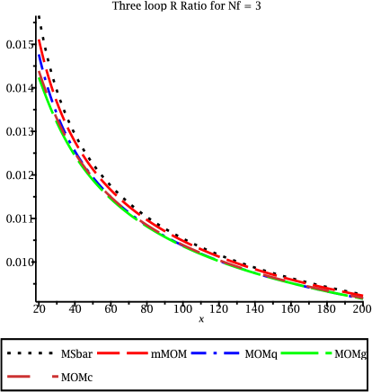
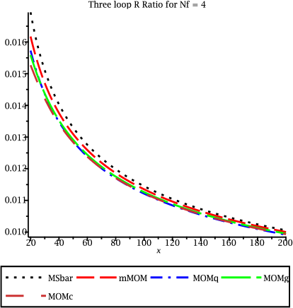
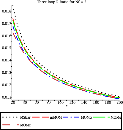
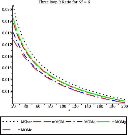
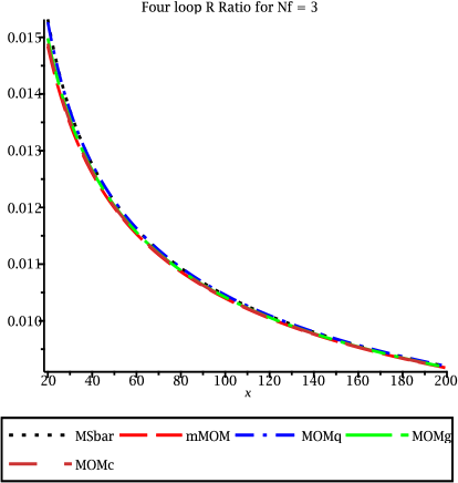
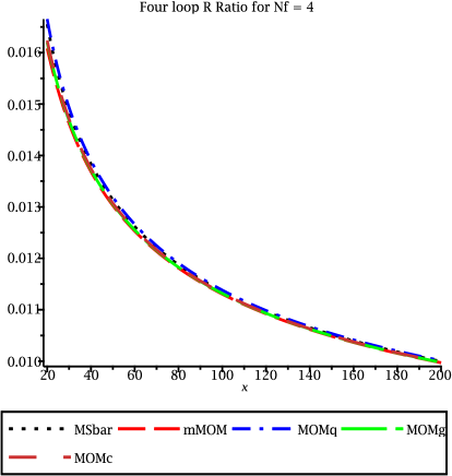
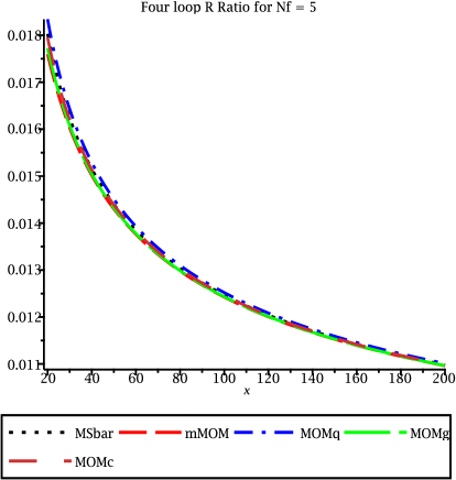
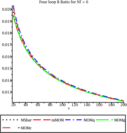
Examining the running of this effective coupling constant across a range of energy values within the perturbative regime will allow us to test whether the trends found in the Tables are specific to the points considered or are more general trends for the series in the range. In order to test our ideas of residual scheme dependence in a measureable due to truncation of a perturbative series we can plot their running across a range of values. In [29] the momentum range chosen was $20\Lambda^{\overline{\mbox{\footnotesize{MS}}}}_{N_{\!f}}$ to $200\Lambda^{\overline{\mbox{\footnotesize{MS}}}}_{N_{\!f}}$ which represented a large part of the perturbative regime especially when $\Lambda^{\overline{\mbox{\footnotesize{MS}}}}_{N_{\!f}}$ was converted to more conventional energy units. In general the value of $\Lambda^{\overline{\mbox{\footnotesize{MS}}}}_{N_{\!f}}$ is larger for higher values of $N_{\!f}$. Therefore the momentum considered in [29] for more active quarks will be lower. This will mean that the effect of truncation will be greater for $N_{\!f}$ $=$ $6$ than for $N_{\!f}$ $=$ $3$. This is counter to what is expected phenomenologically. However we continue with this range to allow for direct comparison with the previous results. It is important to note for instance that due to the particular polynomial dependence on $N_{\!f}$ in different scheme perturbative series for an observable, when it is numerically evaluated certain terms may dominate for one specific number of active quarks but not for another number. How this transpires can be seen when, for example, (2.13) is evaluated for a range of $N_{\!f}$.

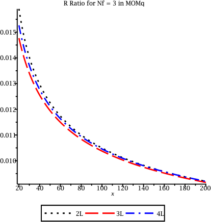
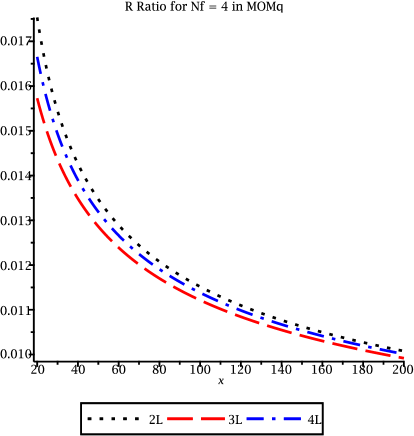
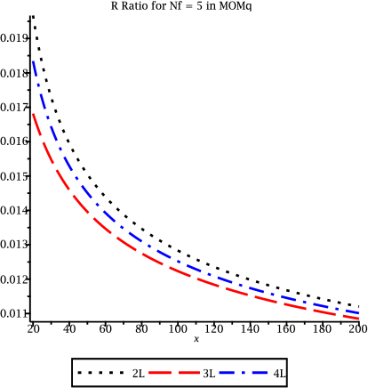
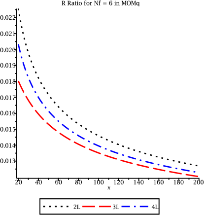
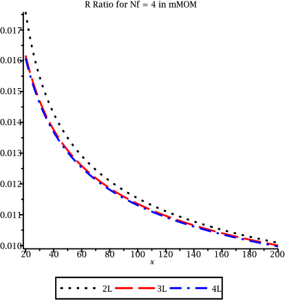
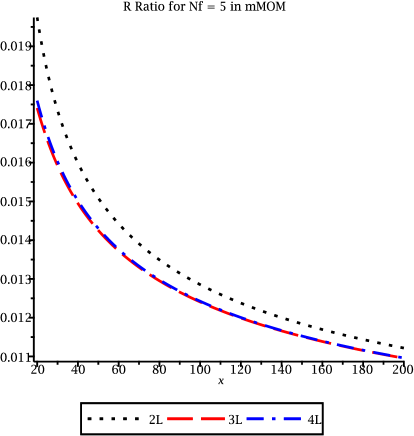
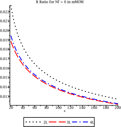
Scheme comparison plots of the R ratio at both $O(a^{3})$ and $O(a^{4})$ are provided in Figures 1 and 2 respectively. For $N_{\!f}$ $=$ $6$ in the $O(a^{4})$ plot we see a very small spread in the value of the series across all momenta, but especially at high momenta where the coupling constant tends to zero meaning higher order corrections are indecipherable. Across the range $20\Lambda^{\overline{\mbox{\footnotesize{MS}}}}$ to $200\Lambda^{\overline{\mbox{\footnotesize{MS}}}}$ the MOMq scheme provides an upper bound on the series, but for the upper bound at $20\Lambda^{\overline{\mbox{\footnotesize{MS}}}}$ the minimum line is that of the mMOM scheme whereas at $200\Lambda^{\overline{\mbox{\footnotesize{MS}}}}$ it is that of the MOMg scheme. Therefore the schemes are differently ordered at different energies. As expected at $N_{\!f}$ $=$ $3$ there is a much smaller, but not non-existent, spread for all the schemes. This is mirrored by the scale of the series in both cases. Note that at no point along the series does MOMg provide the lower bound. So as mentioned the ordering of the series does depend on the value of $N_{\!f}$. For $O(a^{3})$ we see the values of the series are similar when compared with $O(a^{4})$, but provide a much larger spread of values at all energy scales. This is especially prevalent for $N_{\!f}$ $=$ $6$, where the $\overline{\mbox{MS}}$ and mMOM schemes provide bounds, meaning the schemes are not in a fixed order between loop orders.

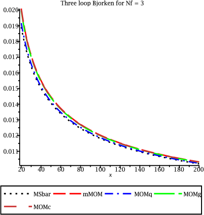
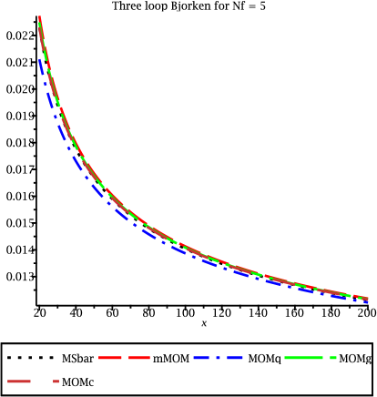
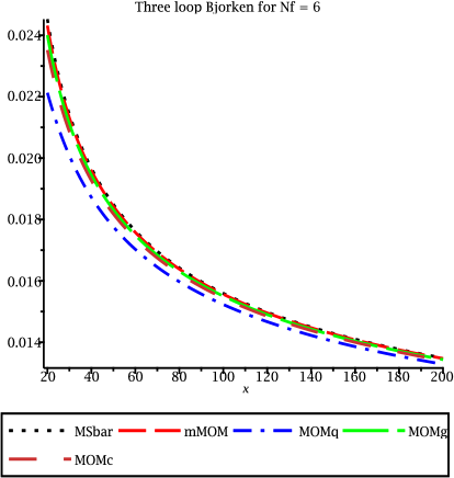
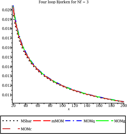
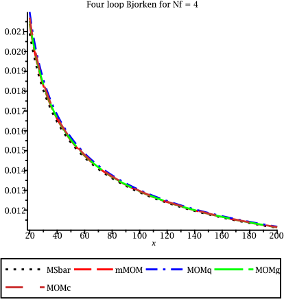
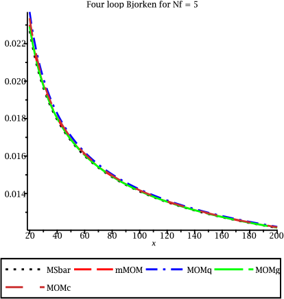
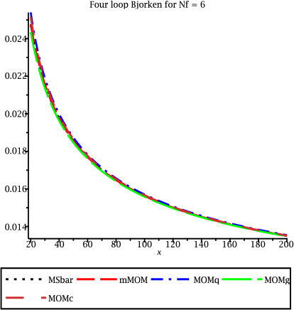
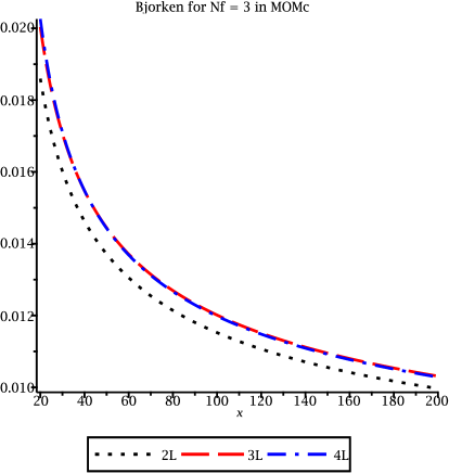
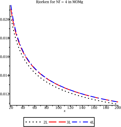
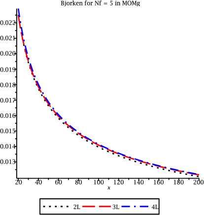
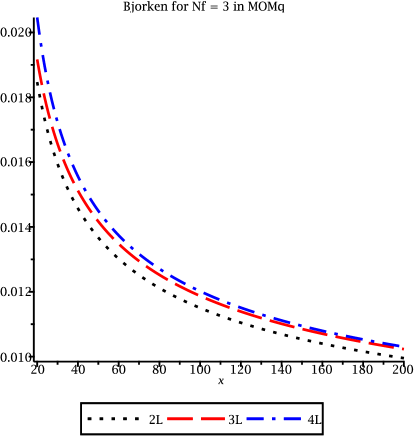
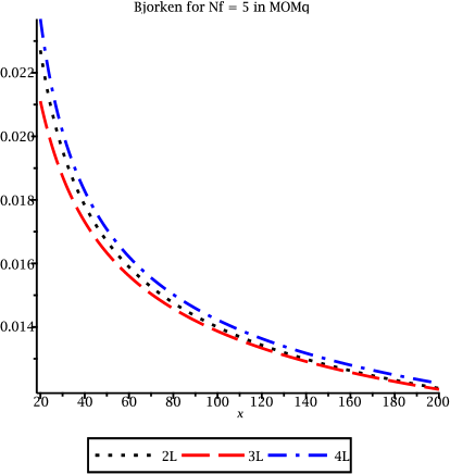
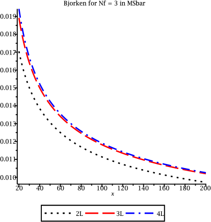
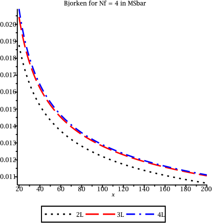
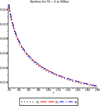
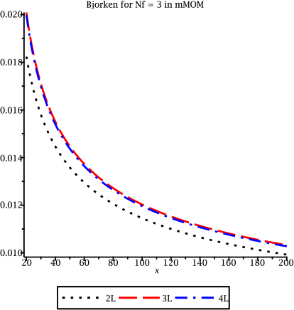
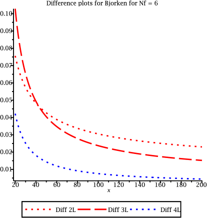
To ensure that any results derived from these graphs are not dependent on the specific observable we have repeated the exercise for the Bjorken sum rule with the behaviour of the effective coupling presented in Figures 3 and 4 for $O(a^{3})$ and $O(a^{4})$ respectively. First considering the $O(a^{4})$ graph we see that the schemes providing the maximum and minimum lines are not the same with $\overline{\mbox{MS}}$ being the minimum for $N_{\!f}$ $=$ $3$. While the scheme difference is in general lower at $O(a^{4})$ than $O(a^{3})$ we see that the jump is not quite as severe. At $O(a^{3})$ it is worth noting that many of the series are highly correlated with just the MOMq scheme behaviour being an outlier at $N_{\!f}$ $=$ $6$ and both the $\overline{\mbox{MS}}$ and MOMq schemes being outliers in the $N_{\!f}$ $=$ $3$ graph.

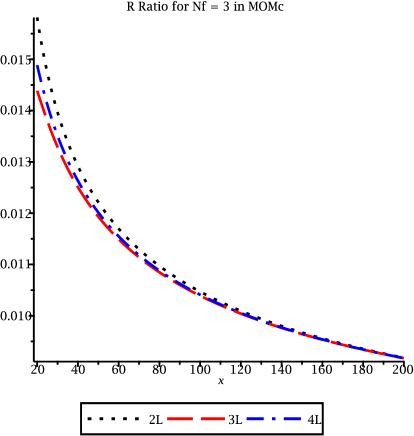
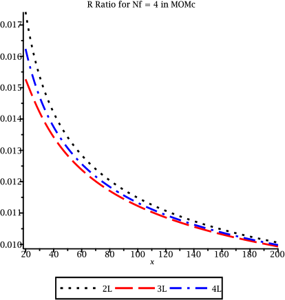
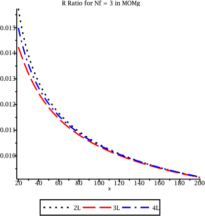
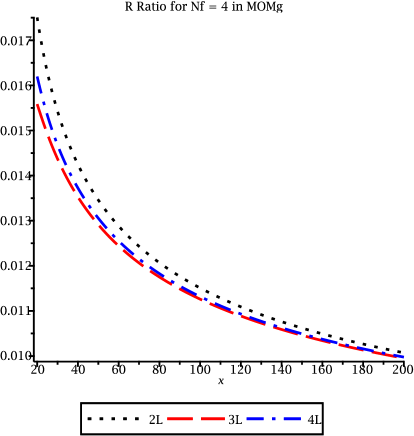
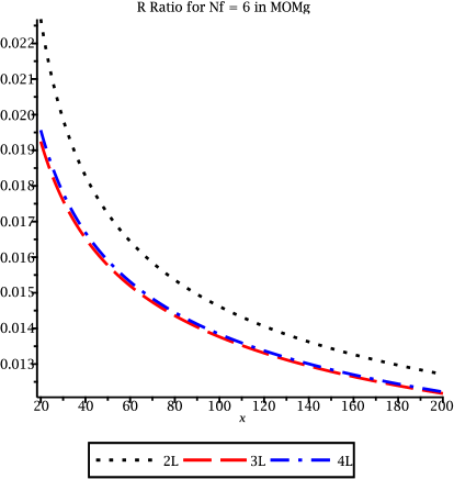
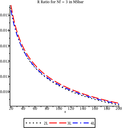
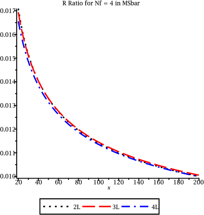
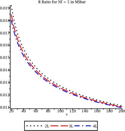
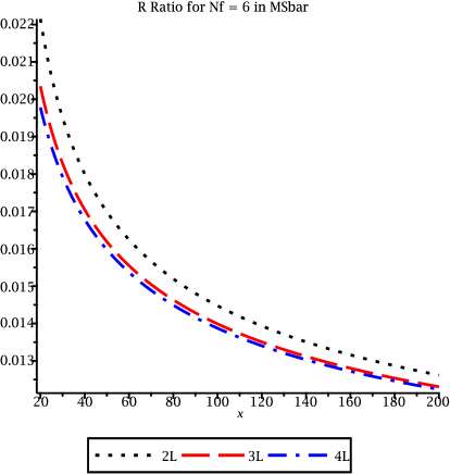
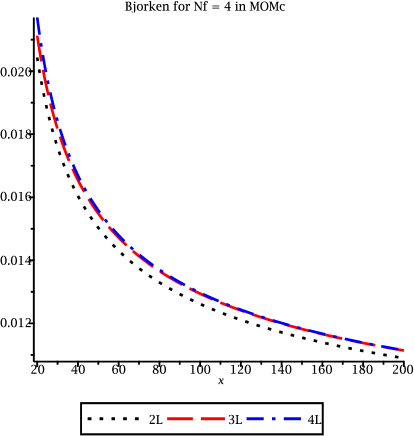
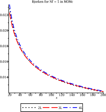
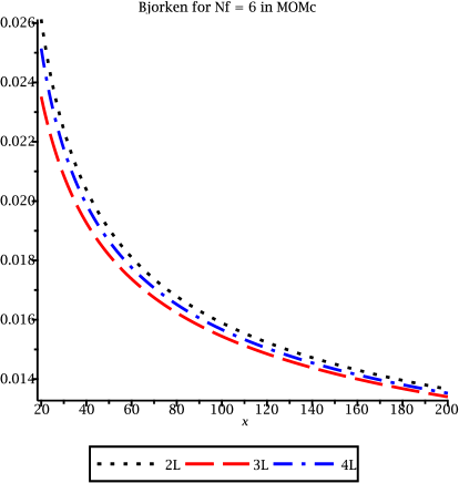
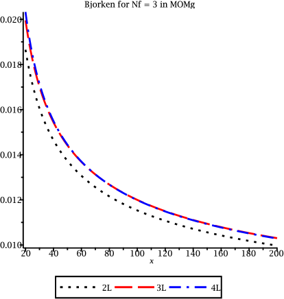
An alternative way of quantifying the behaviour of the observable series is to consider the development of the effective coupling with loop order. Consequentially this will allow for a deeper understanding of how each series converges towards the natural value for each scheme. By plotting the series calculated in a single scheme but at different loop orders together we can gain an understanding of the more general qualitative features of the convergence of each scheme across a larger range. Therefore in Figures 5, 6, 7, 8 and 9 we have provided loop comparisons of the R ratio in the MOMc, MOMg, MOMq, $\overline{\mbox{MS}}$ and mMOM schemes, respectively, for four values of $N_{\!f}$. In the case of MOMc scheme we see the series oscillates as the loop order increases since the $O(a^{4})$ line sits between the two lower order series. The spread of this oscillation decreases with $N_{\!f}$. This behaviour is shared by all other MOMi schemes, whereas the $\overline{\mbox{MS}}$ and mMOM schemes decrease alternating at each order but converging towards a value. In addition the same loop comparisons in each scheme are given for the Bjorken sum rule in Figures 10, 11, 12, 13 and 14. Focussing first on the MOMc convergence, for $N_{\!f}$ $=$ $6$ we see the series oscillates. While this is also seen at high momentum for $N_{\!f}$ $=$ $5$, at low momenta this changes at $O(a^{3})$ in the middle which suggests the breakdown of perturbation theory. Finally for $N_{\!f}$ $=$ $3$ we see that the $O(a^{3})$ and $O(a^{4})$ cases are nearly identical but the $O(a^{2})$ line lies much further below. This general behaviour is shared by the other MOMi schemes.

4 Scheme error.

In quantum field theory typically the calculation of a measureable quantity has no closed form solution. So one must use an approximation often given by a perturbative series in some small quantity. In order to quantify the accuracy of these approximations it is important to assign an error measurement to them. In perturbative QCD measureable quantities are expected to be renormalization group invariant because results in Nature should not be dependent on how we choose to calculate the quantity. One way this is embodied is in scale invariance in which the calculation of a physical observable is expected to be independent of the choice of the renormalization scale. This idea is used to calculate an error estimate with conventional scale setting commonly employed which involves varying the scale, typically by halving and doubling some representative scale of the process. The magnitude the scale is varied by is arbitrary but dictated by what has worked in the past as opposed to some deeper theoretical understanding. It is therefore worthwhile comparing this method to other estimates of the accuracy of a series. Recent reviews of methods to fix scheme and scale ambiguity are given in [49] and [73]. However here we will be using this ambiguity to quantify the uncertainty in theoretical calculations. Renormalization group invariance also implies the invariance of measureable quantities with respect to the choice of renormalization scheme when evaluated to all orders. In this section we formalise the ideas discussed previously to investigate, for contrast, the use of scheme difference as a measure of theoretical error in perturbative QCD. Examples of the use of scheme error in calculations include [51] and [52]. For this study we will assume we have a well-defined renormalization scale.

First we suppose that a measureable quantity $\rho(Q)$ at scale $Q$ has been evaluated up to the $N$-loop level

$$\rho(Q) = \sum_{j=0}^{N}\rho^{\cal S}_{j}a_{\cal S}(Q)^{j}~{}+~{}\Delta(\rho^{\cal S},N,Q)~{}=~{}\rho^{\cal S}_{(N)}(Q)~{}+~{}\Delta(\rho^{\cal S},N,Q)$$ (4.1)

where $\Delta(\rho^{\cal S},N,Q)$ represents the difference between the finite approximation and the true value of the series. Perturbatively it will be $O(a^{N+1})$. Calculating this in schemes ${\cal S}_{1}$ and ${\cal S}_{2}$ gives

$$\rho(Q) = \rho^{{\cal S}_{1}}_{(N)}(Q)~{}+~{}\Delta(\rho^{{\cal S}_{1}},N,Q)~{}=~{}\rho^{{\cal S}_{2}}_{(N)}(Q)~{}+~{}\Delta(\rho^{{\cal S}_{2}},N,Q)~{}.$$ (4.2)

This has two distinct cases, either:

• $\mathbf{sgn}(\Delta(\rho^{{\cal S}_{1}},N,Q))$ $=$ $\mathbf{sgn}(\Delta(\rho^{{\cal S}_{2}},N,Q))$ in which case both $\rho^{{\cal S}_{1}}_{(N)}(Q)$ and $\rho^{{\cal S}_{2}}_{(N)}(Q)$ will produce over- or under-estimates of the true value of the series,

• $\mathbf{sgn}(\Delta(\rho^{{\cal S}_{1}},N,Q))$ $\neq$ $\mathbf{sgn}(\Delta(\rho^{{\cal S}_{2}},N,Q))$ in which case $\rho^{{\cal S}_{1}}_{(N)}(Q)$ and $\rho^{{\cal S}_{2}}_{(N)}(Q)$ will act as bounds on the true value of $\rho(Q)$.

Since in general $\Delta(\rho^{\cal S},N,Q)$ is not known, as this would be equivalent to knowing the true value of the series, we cannot know which case a particular pair of schemes will fit into. However, if we consider more schemes there will be a greater chance that the scheme with the maximum value and the scheme with the minimum value will correctly bound the true value of the series, provided there is no reason to expect additional correlation between the schemes as in the case at the two loop level.

4.1 Scheme envelopes.

Thus far we have discussed how our measure of error may bound the true value without assigning a degree of belief to that bound, a concept which is discussed at length in [74]. One could attempt to consider the values of the schemes to exist in some probability distribution which could then be used to calculate a mean and standard deviation on the series. However no distribution is known. In Section 3 we used the arithmetic mean and unbiased standard deviation which allowed us to provide a rough estimate of the true value of the series and remaining error suggested by the values calculated in each scheme. This had the advantage of allowing one to use the typical interpretation of the standard deviation as a degree of belief in the value reported. However, the use of the arithmetic mean required the assumption that all schemes are independent which due to correlation of the scheme definitions, particularly for the MOMi schemes, is not an accurate assumption. This can be further demonstrated by the qualitative similarity of the convergence of the MOMi schemes and illustrated in the loop comparison graphs. In this subsection we aim to discuss the idea of scheme error more concretely and therefore we have chosen not to make this assumption. So we will not attach any degree of belief to our error.

$\alpha_{s}^{RR}=0.16556\pm 0.01571$
at $Q=31.62278$ GeV
Scheme	Ł	$\alpha_{s}^{\overline{\mbox{\footnotesize{MS}}}}(M_{Z})$
	2	$0.12772^{+0.00948}_{-0.00904}$
$\overline{\mbox{MS}}$	3	$0.13084^{+0.01019}_{-0.00986}$
	4	$0.13187^{+0.01050}_{-0.01027}$
	2	$0.12662^{+0.00923}_{-0.00875}$
mMOM	3	$0.13260^{+0.01083}_{-0.01081}$
	4	$0.13238^{+0.01072}_{-0.01063}$
	2	$0.12680^{+0.00926}_{-0.00879}$
MOMq	3	$0.13460^{+0.01148}_{-0.01171}$
	4	$0.13131^{+0.01030}_{-0.00999}$
	2	$0.12665^{+0.00923}_{-0.00875}$
MOMg	3	$0.13306^{+0.01097}_{-0.01102}$
	4	$0.13228^{+0.01067}_{-0.01054}$
	2	$0.12713^{+0.00934}_{-0.00888}$
MOMc	3	$0.13479^{+0.01171}_{-0.01239}$
	4	$0.13194^{+0.01053}_{-0.01032}$
	2	$0.12717\pm 0.00055^{+0.00948}_{-0.00875}$
Average	3	$0.13281\pm 0.00197^{+0.01171}_{-0.00986}$
	4	$0.13185\pm 0.00053^{+0.01072}_{-0.00999}$

Table 3: Estimates of $\alpha_{s}^{\overline{\mbox{\footnotesize{MS}}}}(M_{Z})$ from the R ratio effective coupling at order Ł using data from [75] calculated in the $\overline{\mbox{MS}}$, MOMi and mMOM schemes. The error on the average is the envelope of the scheme values and the average value is the centre of this envelope.

To give a concrete example we recall that the R ratio effective coupling constants with five active fermions in our five schemes are given numerically by

$$a_{RR}^{\mbox{\footnotesize{mMOM}}}|_{N_{f}=5} = a_{\mbox{\footnotesize{mMOM}}}~{}-~{}2.89086a_{\mbox{\footnotesize{mMOM}}}^{2}~{}-~{}299.03413a_{\mbox{\footnotesize{mMOM}}}^{3}~{}+~{}407.37433a_{\mbox{\footnotesize{mMOM}}}^{4}$$

$$+~{}O(a_{\mbox{\footnotesize{mMOM}}}^{5})$$

$$a_{RR}^{\mbox{\footnotesize{MOMc}}}|_{N_{f}=5} = a_{\mbox{\footnotesize{MOMc}}}~{}-~{}7.35580a_{\mbox{\footnotesize{MOMc}}}^{2}~{}-~{}258.15390a_{\mbox{\footnotesize{MOMc}}}^{3}~{}+~{}3883.57250a_{\mbox{\footnotesize{MOMc}}}^{4}$$

$$+~{}O(a_{\mbox{\footnotesize{MOMc}}}^{5})$$

$$a_{RR}^{\mbox{\footnotesize{MOMg}}}|_{N_{f}=5} = a_{\mbox{\footnotesize{MOMg}}}~{}-~{}3.77154a_{\mbox{\footnotesize{MOMg}}}^{2}~{}-~{}275.52688a_{\mbox{\footnotesize{MOMg}}}^{3}~{}+~{}1671.72909a_{\mbox{\footnotesize{MOMg}}}^{4}$$

$$+~{}O(a_{\mbox{\footnotesize{MOMg}}}^{5})$$

$$a_{RR}^{\mbox{\footnotesize{MOMq}}}|_{N_{f}=5} = a_{\mbox{\footnotesize{MOMq}}}~{}-~{}5.52330a_{\mbox{\footnotesize{MOMq}}}^{2}~{}-~{}168.45783a_{\mbox{\footnotesize{MOMq}}}^{3}~{}+~{}1337.29074a_{\mbox{\footnotesize{MOMq}}}^{4}$$

$$+~{}O(a_{\mbox{\footnotesize{MOMq}}}^{5})$$

$$a_{RR}^{\overline{\mbox{\footnotesize{MS}}}}|_{N_{f}=5} = a_{\overline{\mbox{\footnotesize{MS}}}}~{}+~{}5.63692a_{\overline{\mbox{\footnotesize{MS}}}}^{2}~{}-~{}204.27304a_{\overline{\mbox{\footnotesize{MS}}}}^{3}~{}-~{}5118.76040a_{\overline{\mbox{\footnotesize{MS}}}}^{4}$$ (4.3)

$$+~{}O(a_{\overline{\mbox{\footnotesize{MS}}}}^{5})~{}.$$

These have been derived from the R ratio perturbative series using the notation of (3.7). For a valid perturbative series at the $N$-th loop level we expect $\Delta(\rho^{\cal S},N,Q)$ to be dominated by the $(N+1)$-th term in the original series. By considering the sign of the third term in each series we get a rough estimate of the $\Delta$-value at the two loop level for instance. Since each sign is negative this means that each value calculated at $O(a^{2})$ will be an over-estimate of the series, which explains the lower scheme difference at the two loop level when compared to three loops. This should provide an accurate error since the signs are different on the $O(a^{4})$ terms in each series. Since we do not know the five loop terms in any series the signs of the $\Delta$-values at the four loop level cannot be known exactly. However there is no reason to expect all five schemes to share the same sign at that loop level. We can therefore consider the envelope provided by the $O(a^{3})$ lines of the plots as an absolute limit on the true value of the series with the lines provided by the $O(a^{4})$ values as the potential minimum error at that order. We note that this argument is simplified for clarity as it ignores the modification of the coupling constant at each order. Although as discussed previously the dominant term is typically from the new term in the series.

$\alpha_{s}^{RR}=0.14546\pm 0.01382$
at $Q=59.16080$ GeV
Scheme	Ł	$\alpha_{s}^{\overline{\mbox{\footnotesize{MS}}}}(M_{Z})$
	2	$0.12731^{+0.01070}_{-0.01045}$
$\overline{\mbox{MS}}$	3	$0.13004^{+0.01136}_{-0.01122}$
	4	$0.13085^{+0.01162}_{-0.01156}$
	2	$0.12636^{+0.01047}_{-0.01017}$
mMOM	3	$0.13124^{+0.01180}_{-0.01185}$
	4	$0.13116^{+0.01175}_{-0.01176}$
	2	$0.12651^{+0.01051}_{-0.01021}$
MOMq	3	$0.13273^{+0.01229}_{-0.01252}$
	4	$0.13048^{+0.01148}_{-0.01136}$
	2	$0.12638^{+0.01047}_{-0.01017}$
MOMg	3	$0.13159^{+0.01191}_{-0.01200}$
	4	$0.13111^{+0.01172}_{-0.01172}$
	2	$0.12680^{+0.01058}_{-0.01029}$
MOMc	3	$0.13264^{+0.01233}_{-0.01269}$
	4	$0.13089^{+0.01163}_{-0.01159}$
	2	$0.12683\pm 0.00048^{+0.01070}_{-0.01017}$
Average	3	$0.13138\pm 0.00135^{+0.01229}_{-0.01122}$
	4	$0.13082\pm 0.00034^{+0.01175}_{-0.01136}$

Table 4: Estimates of $\alpha_{s}^{\overline{\mbox{\footnotesize{MS}}}}(M_{Z})$ from the R ratio effective coupling at order Ł using data from [75] calculated in the $\overline{\mbox{MS}}$, MOMi and mMOM schemes. The error on the average is the envelope of the scheme values and the average value is the centre of this envelope.

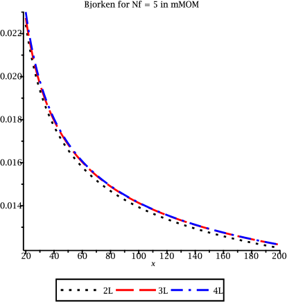
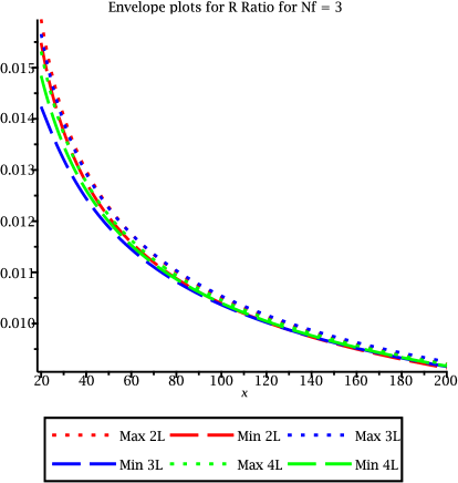
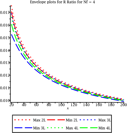
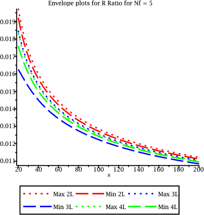
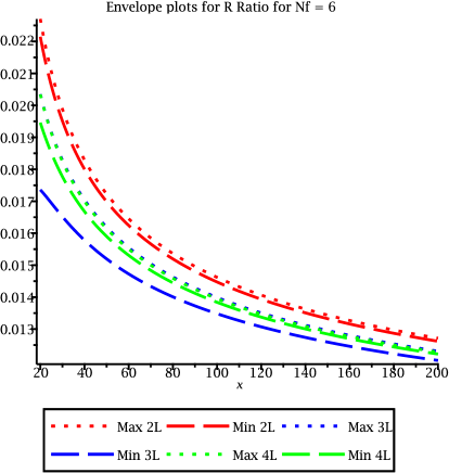
With this in mind we compare the envelopes for the R ratio effective coupling constants at the different loop orders against each other in Figure 15. At each energy scale all schemes are considered but only the ones that evaluate to give the minimum and maximum values are plotted at each point. We note that as discussed in Section 3 the bounding schemes can change between loop order, at different energies and for different $N_{\!f}$. This means that all schemes must be considered at all values for an accurate envelope to be formed. For the case of six active fermions we see that the two loop envelope sits entirely above the three loop envelope which houses the four loop at its upper bound. The fact that there is no overlap between the three and four loop cases is explained by the fact that the three loop term acts to reduce the value of the R ratio in all of the schemes considered here. For the situation with three active fermions there exists an overlap between the three loop and four loop graphs, although at lower energies while the four loop lies inside the three loop it is not within the two loop envelope. At higher energies however the two and three loop envelopes lie on top of each other with the four loop one lying in between. In general we see that the two loop and four loop envelopes are of similar size, with that at three loops giving a larger bound.

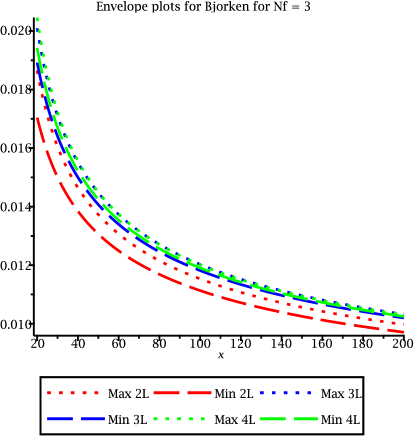
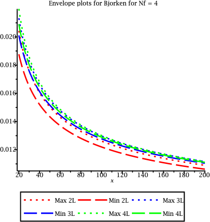
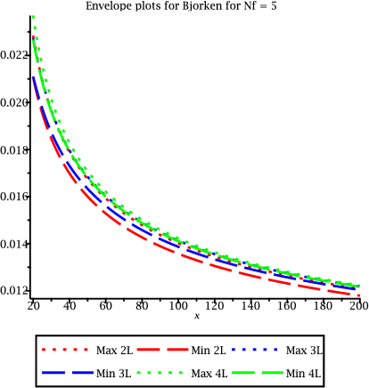
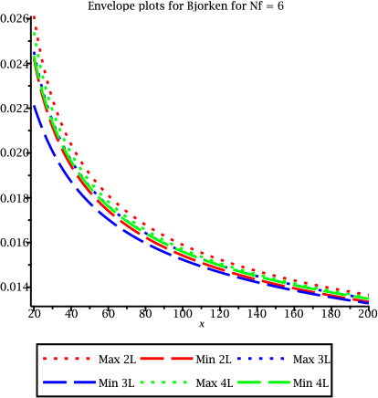
This can be contrasted with similar plots for the Bjorken sum rule given in Figure 16. Starting with the case of three active fermions the $O(a^{2})$ error is entirely below and much larger than the $O(a^{3})$ bound. The full $O(a^{4})$ envelope is within the $O(a^{3})$ envelope at higher energies but at lower energies the upper bound just escapes. As the number of active fermions is increased both the two loop and four loop lines increase relative to the three loop one. So for six active fermions the two loop envelope lies almost entirely above the three loop one and the four loop lower bound sits on the upper bound of the three loop. In that case the four loop one is encapsulated by the two loop one but not the three loop one, suggesting that the two loop case gives a more accurate maximum envelope than the three loop one.

$\alpha_{s}^{RR}=0.13697\pm 0.01225$
at $Q=82.15838$ GeV
Scheme	Ł	$\alpha_{s}^{\overline{\mbox{\footnotesize{MS}}}}(M_{Z})$
	2	$0.12725^{+0.01066}_{-0.01053}$
$\overline{\mbox{MS}}$	3	$0.12982^{+0.01126}_{-0.01124}$
	4	$0.13056^{+0.01149}_{-0.01154}$
	2	$0.12635^{+0.01044}_{-0.01027}$
mMOM	3	$0.13085^{+0.01162}_{-0.01174}$
	4	$0.13081^{+0.01159}_{-0.01169}$
	2	$0.12650^{+0.01048}_{-0.01031}$
MOMq	3	$0.13216^{+0.01203}_{-0.01230}$
	4	$0.13024^{+0.01137}_{-0.01137}$
	2	$0.12637^{+0.01045}_{-0.01028}$
MOMg	3	$0.13115^{+0.01171}_{-0.01187}$
	4	$0.13077^{+0.01157}_{-0.01166}$
	2	$0.12677^{+0.01054}_{-0.01039}$
MOMc	3	$0.13201^{+0.01203}_{-0.01237}$
	4	$0.13059^{+0.01150}_{-0.01156}$
	2	$0.12680\pm 0.00045^{+0.01066}_{-0.01027}$
Average	3	$0.13099\pm 0.00117^{+0.01203}_{-0.01124}$
	4	$0.13053\pm 0.00028^{+0.01159}_{-0.01137}$

Table 5: Estimates of $\alpha_{s}^{\overline{\mbox{\footnotesize{MS}}}}(M_{Z})$ from the R ratio effective coupling at order Ł using data from [75] calculated in the $\overline{\mbox{MS}}$, MOMi and mMOM schemes. The error on the average is the envelope of the scheme values and the average value is the centre of this envelope.

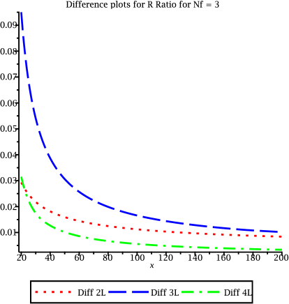
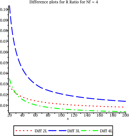
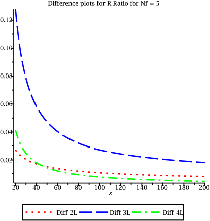
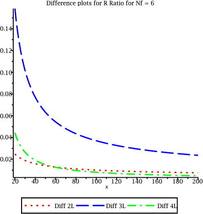
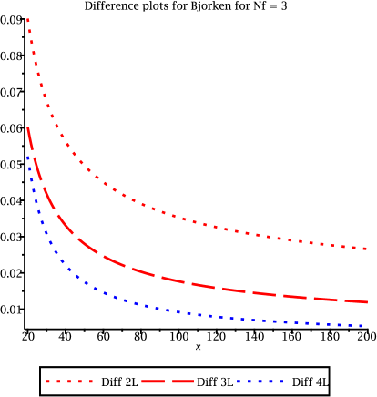
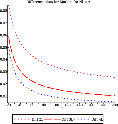
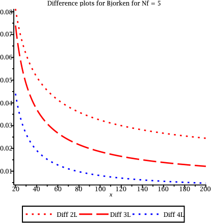
Instead of considering the envelopes themselves we can examine the difference between the maximum and minimum values in the envelope, as normalized by the midpoint of the envelope. This will provide a clearer display of the remaining scheme dependence. This is presented in Figure 17 for the R ratio with Figure 18 giving the corresponding situation for the Bjorken sum rule. As discussed earlier, for the R ratio we see in general the scheme difference at $O(a^{3})$ is largest, at $O(a^{4})$ it is smallest for most of the range considered except at very low momenta where the $O(a^{2})$ difference is smaller. For example, at $x$ $=$ $110$ for $N_{\!f}$ $=$ $5$ the $O(a^{2})$ difference is $1.0\%$, the $O(a^{3})$ is $2.5\%$ and the $O(a^{4})$ is $0.7\%$. The Bjorken sum rule provides a more conventional error for a perturbative series where in general the $O(a^{2})$ error is larger than the $O(a^{3})$ error which in turn is larger than the $O(a^{4})$ error.

$\alpha_{s}^{{\mbox{\footnotesize{Bjr}}}}=0.70800\pm 0.25716$
at $Q=1.64500$ GeV
Scheme	Ł	$\alpha^{\overline{\mbox{\footnotesize{MS}}}}(M_{Z})$
	2	$0.12819^{+0.01064}_{-0.00538}$
$\overline{\mbox{MS}}$	3	$0.12665^{+0.01101}_{-0.00574}$
	4	$0.12320^{+0.00973}_{-0.00498}$
	2	$0.12228^{+0.00847}_{-0.00403}$
mMOM	3	$0.12395^{+0.00952}_{-0.00536}$
	4	$0.12025^{+0.00749}_{-0.00328}$
	2	$0.12080^{+0.00795}_{-0.00374}$
MOMq	3	$-$
	4	$0.11752^{+0.00659}_{-0.00291}$
	2	$0.12340^{+0.00823}_{-0.00388}$
MOMg	3	$-$
	4	$0.12185^{+0.00700}_{-0.00279}$
	2	$0.12003^{+0.00768}_{-0.00364}$
MOMc	3	$-$
	4	$0.11752^{+0.00614}_{-0.00229}$
	2	$0.12411\pm 0.00408^{+0.01064}_{-0.00364}$
Average	3	$\left[\frac{}{}0.12530\pm 0.00135^{+0.00536}_{-0.01101}\right]$
	4	$0.12036\pm 0.00284^{+0.00973}_{-0.00229}$

Table 6: Estimates of $\alpha_{s}^{\overline{\mbox{\footnotesize{MS}}}}(M_{Z})$ from the Bjorken sum rule effective coupling at order Ł using data from [76, 77] calculated in the $\overline{\mbox{MS}}$, MOMi and mMOM schemes. The error on the average is the envelope of the scheme values and the average value is the centre of this envelope. The bracketed error indicates an envelope formed with the incomplete set of schemes.

4.2 Estimating formal parameters.

As a final quantitative scheme comparison we consider the fundamental formal parameters of the theory calculated using experimental data. In massless perturbative QCD the $\Lambda$-parameter or equivalently the coupling constant defined at a particular renormalization scale are the only parameters that must be inserted in order to make physical calculations. One can use the $\Lambda$-ratio or the coupling constant conversion functions to compare quantities calculated in each scheme in order to investigate residual scheme dependence. The most often quoted value is the coupling constant in the $\overline{\mbox{MS}}$ scheme evaluated at the mass of the $Z$ boson. Therefore that parameter, $\alpha_{s}^{\overline{\mbox{\footnotesize{MS}}}}(M_{Z})$, will be considered here. We note that in Nature resonances in partial interactions at any mass scale will be present and reflected in associated experimental data. Such phenomena are not accounted for in a massless theory. Therefore this study should also be regarded as part of a theory laboratory where we are particularly interested and can focus on the scheme dependence of the final result in a controlled setup rather than the precise value itself.

$\alpha_{s}^{{\mbox{\footnotesize{Bjr}}}}=0.61700\pm 0.25410$
at $Q=1.79500$ GeV
Scheme	Ł	$\alpha^{\overline{\mbox{\footnotesize{MS}}}}(M_{Z})$
	2	$0.12736^{+0.01470}_{-0.00686}$
$\overline{\mbox{MS}}$	3	$0.12559^{+0.01488}_{-0.00726}$
	4	$0.12242^{+0.01335}_{-0.00631}$
	2	$0.12194^{+0.01211}_{-0.00522}$
mMOM	3	$0.12331^{+0.01315}_{-0.00640}$
	4	$0.12019^{+0.01106}_{-0.00437}$
	2	$0.12057^{+0.01147}_{-0.00485}$
MOMq	3	$-$
	4	$0.11762^{+0.00984}_{-0.00384}$
	2	$0.12319^{+0.01188}_{-0.00503}$
MOMg	3	$0.12863^{+0.01538}_{-0.02879}$
	4	$0.12210^{+0.01077}_{-0.00384}$
	2	$0.11986^{+0.01112}_{-0.00470}$
MOMc	3	$-$
	4	$0.11784^{+0.00959}_{-0.00321}$
	2	$0.12361\pm 0.00375^{+0.01470}_{-0.00470}$
Average	3	$\left[\frac{}{}0.12597\pm 0.00266^{+0.01538}_{-0.02347}\right]$
	4	$0.12002\pm 0.00240^{+0.01335}_{-0.00384}$

Table 7: Estimates of $\alpha_{s}^{\overline{\mbox{\footnotesize{MS}}}}(M_{Z})$ from the Bjorken sum rule effective coupling at order Ł using data from [76, 77] calculated in the $\overline{\mbox{MS}}$, MOMi and mMOM schemes. The error on the average is the envelope of the scheme values and the average value is the centre of this envelope. The bracketed error indicates an envelope formed with the incomplete set of schemes.

We will use an experimental measurement for one of our perturbative series $\rho^{*}$ which was found at a particular energy level $Q^{*}$. With the series evaluated in a given scheme we can numerically solve for the $\Lambda$-parameter by varying $\Lambda^{\cal S}$ in

$$\rho^{*}~{}=~{}\rho^{\cal S}({Q^{*}},{\Lambda^{\cal S}_{N_{\!f}}})~{}.$$ (4.4)

If in running from $Q^{*}$ to $M_{Z}$ we cross any threshold $T$ that exists in the massive theory we still consider the massless case but we change the number of active fermions. For example, say there are $N_{\!f}$ active fermions at $Q^{*}$ but in running to $M_{Z}$ we cross the mass threshold where the next quark becomes active at mass $M_{T}$ then we have to accommodate $N_{\!f}+1$ active quarks in the analysis beyond $M_{T}$. We can find the value of the coupling constant at the threshold explicitly by substituting $M_{T}$ and the value found for $\Lambda^{\cal S}_{N_{\!f}}$ into the explicit formula for the coupling constant given in (3). We consider the coupling constant to change continuously at the threshold and therefore we solve

$$a^{\cal S}(M_{T},\Lambda^{\cal S}_{N_{\!f}})~{}=~{}a^{\cal S}(M_{T},\Lambda^{\cal S}_{N_{\!f}+1})$$ (4.5)

numerically for $\Lambda^{\cal S}_{N_{\!f}+1}$. This process is repeated until there are five current active fermions which is the number of active fermions at $M_{Z}$. We note that a similar process could be used to move down below a mass threshold as well. Finally, we evaluate $a^{\cal S}(M_{Z}/\Lambda^{\cal S}_{5})$ explicitly and substitute the value into the coupling constant conversion function in order to have a value to compare between the schemes.

$\alpha_{s}^{{\mbox{\footnotesize{Bjr}}}}=0.58100\pm 0.22308$
at $Q=1.96700$ GeV
Scheme	Ł	$\alpha^{\overline{\mbox{\footnotesize{MS}}}}(M_{Z})$
	2	$0.12812^{+0.01423}_{-0.00711}$
$\overline{\mbox{MS}}$	3	$0.12620^{+0.01433}_{-0.00747}$
	4	$0.12310^{+0.01289}_{-0.00650}$
	2	$0.12284^{+0.01180}_{-0.00546}$
mMOM	3	$0.12412^{+0.01274}_{-0.00649}$
	4	$0.12119^{+0.01084}_{-0.00464}$
	2	$0.12151^{+0.01120}_{-0.00508}$
MOMq	3	$-$
	4	$0.11866^{+0.00966}_{-0.00406}$
	2	$0.12417^{+0.01161}_{-0.00528}$
MOMg	3	$0.12907^{+0.01453}_{-0.03158}$
	4	$0.12330^{+0.01067}_{-0.00417}$
	2	$0.12081^{+0.01087}_{-0.00492}$
MOMc	3	$-$
	4	$0.11896^{+0.00948}_{-0.00350}$
	2	$0.12446\pm 0.00365^{+0.01423}_{-0.00492}$
Average	3	$\left[\frac{}{}0.12660\pm 0.00248^{+0.01453}_{-0.02663}\right]$
	4	$0.12098\pm 0.00232^{+0.01067}_{-0.00406}$

Table 8: Estimates of $\alpha_{s}^{\overline{\mbox{\footnotesize{MS}}}}(M_{Z})$ from the Bjorken sum rule effective coupling at order Ł using data from [76, 77] calculated in the $\overline{\mbox{MS}}$, MOMi and mMOM schemes. The error on the average is the envelope of the scheme values and the average value is the centre of this envelope. The bracketed error indicates an envelope formed with the incomplete set of schemes.

In practice we have utilised the $\Lambda$-ratio and a numerical root finding algorithm to search for the value of $\Lambda^{\overline{\mbox{\footnotesize{MS}}}}$ which would result in the correct value of the R ratio at a given energy level. A fixed range for $\Lambda^{\overline{\mbox{\footnotesize{MS}}}}$ of $50-800$ MeV has been chosen to cover much of the perturbative regime, where we expect $\Lambda^{\overline{\mbox{\footnotesize{MS}}}}$ $\sim$ $200$ MeV [70]. A root bisection algorithm was used to find the value of $y$ that gives the solution of

$$\rho^{*}-\rho^{\cal S}\Bigg{(}Q^{*}\frac{\Lambda^{\overline{\mbox{\footnotesize{MS}}}}}{\Lambda^{\cal S}},y\Bigg{)}~{}=~{}0~{}.$$ (4.6)

where ${\cal S}$ may be any of the schemes considered including $\overline{\mbox{MS}}$ in which the above $\Lambda$-ratio to the $\overline{\mbox{MS}}$ scheme is unity. As the numerical $\Lambda$ value is intermediate to our analysis care was taken to ensure the result was sufficiently accurate for further calculations.

$\alpha_{s}^{{\mbox{\footnotesize{Bjr}}}}=0.63600\pm 0.18702$
at $Q=2.17700$ GeV
Scheme	Ł	$\alpha^{\overline{\mbox{\footnotesize{MS}}}}(M_{Z})$
	2	$0.13287^{+0.00957}_{-0.00564}$
$\overline{\mbox{MS}}$	3	$0.13093^{+0.00979}_{-0.00594}$
	4	$0.12741^{+0.00866}_{-0.00514}$
	2	$0.12691^{+0.00768}_{-0.00429}$
mMOM	3	$0.12852^{+0.00853}_{-0.00521}$
	4	$0.12498^{+0.00685}_{-0.00360}$
	2	$0.12542^{+0.00722}_{-0.00398}$
MOMq	3	$-$
	4	$0.12215^{+0.00601}_{-0.00314}$
	2	$0.12826^{+0.00750}_{-0.00414}$
MOMg	3	$0.13502^{+0.01105}_{-0.02911}$
	4	$0.12715^{+0.00657}_{-0.00320}$
	2	$0.12464^{+0.00698}_{-0.00386}$
MOMc	3	$-$
	4	$0.12235^{+0.00571}_{-0.00263}$
	2	$0.12876\pm 0.00411^{+0.00957}_{-0.00386}$
Average	3	$\left[\frac{}{}0.13177\pm 0.00325^{+0.01105}_{-0.00325}\right]$
	4	$0.12478\pm 0.00263^{+0.00866}_{-0.00314}$

Table 9: Estimates of $\alpha_{s}^{\overline{\mbox{\footnotesize{MS}}}}(M_{Z})$ from the Bjorken sum rule effective coupling at order Ł using data from [76, 77] calculated in the $\overline{\mbox{MS}}$, MOMi and mMOM schemes. The error on the average is the envelope of the scheme values and the average value is the centre of this envelope. The bracketed error indicates an envelope formed with the incomplete set of schemes.

We recall that the world average value of the effective coupling constant at the mass of the $Z$ boson is $\alpha_{s}^{\overline{\mbox{\footnotesize{MS}}}}(M_{Z})$ $=$ $0.1179$ $\pm$ $0.0009$ [78] where $\alpha_{s}^{\overline{\mbox{\footnotesize{MS}}}}$ $=$ $4\pi a_{\overline{\mbox{\footnotesize{MS}}}}$. Since this coupling constant is more commonly used we have chosen to display our results with this convention. Converting the R ratio data given in [75] to our effective coupling constant and using the above described method for finding $\alpha_{s}^{\overline{\mbox{\footnotesize{MS}}}}(M_{Z})$ in each scheme with the data our results are recorded in Tables 3, 4 and 5 which use experimental data from [75]. The values given at each loop order in each scheme are for the central experimental value. The errors are found by solving for the upper and lower bounds on the experimental value. We have added an additional row for each loop order giving the average value of the other scheme values at that loop order. As a scheme distribution is not known we have chosen to use the central value of the envelopes as the average with the first error being the theory error from the scheme difference envelope and the upper and lower bound on the second error being the experimental error on the maximum and minimum central value from the schemes, respectively.

In Tables 3, 4 and 5 we see the general trend discussed before where the scheme error at two loops increases drastically at three loops and then decreases below the two loop error at four loops. We note that the values calculated for $\alpha_{s}^{\overline{\mbox{\footnotesize{MS}}}}$ are larger than the current world average. However since we are considering massless QCD some difference is expected and the values found here are commensurate with similar analysis made using the same data in [49]. Despite our unphysical assumptions, this analysis does show that the general trend of reduced scheme dependence at the four loop level can translate to reduced theory error in formal quantities calculated with experimental data. On general field theoretical grounds this is not unexpected but the analysis has provided a degree of quantification.

We have repeated this exercise for the Bjorken sum rule using data from [76, 77] with the results given in Tables 6, 7, 8 and 9. In this case we used the higher $Q^{2}$ values of the effective coupling constant presented in Table I of [46] derived from the deeply virtual Compton scattering measurement of the sum rule recorded in [76, 77]. Due to the low energies considered in this case these data points push the boundaries of validity for the perturbative regime. Therefore a three loop estimate could not be made for one or more instances for the symmetric momentum subtraction schemes as their three loop series do not meet the experimental effective coupling constant value. Although, this reduced scheme error at three loops compared with the two loop result is consistent with our difference plots of the running of the Bjorken sum rule in different schemes provided in Figure 18. The smaller error on the three loop average values can then be understood as due to the reduction in the schemes considered, especially since the $\overline{\mbox{MS}}$ and mMOM ones are related as described earlier. Importantly though the scheme dependence is again reduced at the four loop level. Indeed for the higher $Q^{2}$ values in the Bjorken case the four loop error for what is termed the average, which includes the MOM schemes, is compatible if not better than the three loop average. In other words the fact that all schemes provide results at four loops, despite not giving results at three loops, could be interpreted as the series settling down at the new loop level. However it may be the case that this is simply due to the fact this is at the interface of perturbative reliability for low loop order. So there is a large contribution at the four loop level which is positive in all cases meaning the term that will dominate as the $\Lambda$-parameter is decreased will increase the value of the effective coupling constant which in turn means the series will increase above the experimental values. Overall the values found from the Bjorken data are much lower than those of the R ratio, with the Bjorken data being closer to the current world average.

5 Discussion.

We have completed a comprehensive investigation into the scheme dependence of two observables at as high a loop order as is presently possible. This included the kinematic schemes of [20, 21] which are based on a specific momentum configuration of the core $3$-point vertices of QCD. Our main aim was to quantify the error on a benchmark parameter, $\alpha_{s}^{\overline{\mbox{\footnotesize{MS}}}}(M_{Z})$, that was more field theoretically based and accounted for the uncertainty that is inherent in the truncation of the perturbation series in different schemes. We stress that our formulation was in the idealized and purely theoretical situation where quark masses and threshold effects were not included. We remark parenthetically, however, that in the former instance a hybrid or partial MOM scheme investigation could be instigated in the approximation of heavy mass corrections, such as [79] which includes the Bjorken sum rule, since the coupling constant and quark mass, treated as parameters, can be mapped from the $\overline{\mbox{MS}}$ scheme to one of the MOMi ones from available data. The construction is termed hybrid or partial in the sense that the MOMi scheme maps do not include quark masses but would have an approximation in a heavy quark mass. Further, while recognizing that our massless investigation is not realistic on the contrary it allowed us to focus purely on the effect corrections in different schemes have in a controlled scenario. Although the central value for $\alpha_{s}^{\overline{\mbox{\footnotesize{MS}}}}(M_{Z})$ differed for the two cases of the Bjorken sum rule and the R ratio what was generally apparent is that with increasing loop order there was a narrowing of our error estimates and an indication of convergence. For the various schemes we concentrated on this improvement was prevalent at four and higher orders which is encouraging. Moreover that in itself justifies the need to progress the renormalization of QCD in MOMi schemes to the next order. To improve our error analysis further more data and additional schemes could be considered. Here we concentrated on the mMOM, $\overline{\mbox{MS}}$ and MOMi schemes, many of which are related via the renormalization group construction meaning that the final results from each scheme cannot be considered as independent. Indeed they are very much connected via the underlying properties of the renormalization group equation. In addition to this much of the data considered is outside the range where perturbation theory is ordinarily applied, particularly for the Bjorken sum rule. So considering more data in the perturbative regime should provide more accurate information on scheme dependence. Additional investigation of the scheme distribution could further inform our results allowing for a better average and degree of belief to be attached to our error estimates.

Aside from the fully symmetric point schemes of [20, 21] considered here there are extensions of those to more general kinematic schemes. For instance, one variation of [20, 21] was introduced in [80, 81] where a parameter $\omega$ reflected the relative weighting of the external momentum flowing through one of the legs of the $3$-point vertices. Such a parameter would naturally translate to a suite of schemes generalizing those of [20, 21]. As the range of $\omega$ is limited to $\omega$ $\in$ $(0,4)$, with the bounding values originating from infrared or colinear singularities, then $\omega$ could provide a more natural way to tune or quantify the range of theoretical errors deriving from an application of the approach discussed here. Equally rather than have one controlling parameter we recall that there are three independent variables for an off-shell $3$-point vertex. These are one overall scale and two dimensionless momenta ratios which, like $\omega$, are bounded but in this instance the dimensionless variables are constrained to lie within a paraboloid. While this too could translate to a bounding region on theory errors of an observable only the underlying two loop massless off-shell master integrals are available at present [28, 62, 64, 65, 82]. Knowledge of the three loop fully off-shell masters would be needed before a concrete analysis of this extensions could proceed. Moreover if achieved it would be of interest to compare with other methods of extracting scale independent information from observables. Ultimately it ought to be the case that with high enough loop order information all well-founded methods of determining scale independent results for an observable should themselves converge to the same value. Another direction that was briefly considered in [29] was the inclusion of the gauge parameter in the evolution of the effective coupling derived from the R ratio in the MOM schemes. Such dependence could equally be embedded in an error analysis. However before that could proceed to the order considered here the renormalization group functions in the three MOM schemes would have to be determined for non-zero $\alpha$. Currently only the four loop Landau gauge expressions are available [24]. Finally, in the more immediate future extending the present work to the five loop level would provide further insight into whether the scale of reduction in scheme dependence is due to an artifact of the underlying scheme used at the four loop level or because it is due to true scheme independence. In the short term it would seem that all the technology to analytically compute the four loop massless symmetric $3$-point master Feynman integrals is actually available. For instance, the first step of carrying out the momentum expansion of the four loop masters to high order is viable now that the four loop Forcer algorithm, [83, 84], written in Form, [60, 61], has superseded the three loop Mincer package.

Acknowledgements. This work was supported in part by a DFG Mercator Fellowship (JAG), STFC Consolidated Grant ST/T000988/1 (JAG) and an EPSRC Studentship EP/R513271/1 (RHM). For the purpose of open access, the authors have applied a Creative Commons Attribution (CC-BY) licence to any Author Accepted Manuscript version arising. The electronic versions representing the Landau gauge expressions for the Bjorken sum rule and R ratio in the mMOM and MOMi schemes used here are accessible from the arXiv ancillary directory associated with the article. The symbolic manipulation language Form, [60, 61], was employed for various calculations in this article. RHM thanks A. Freitas and T. Teubner for useful conversations.

Figure 1: Comparison of $a_{RR}^{\cal S}(x)$ at three loops for the various schemes for $N_{\!f}$ $=$ $3$, $4$, $5$ and $6$.

Figure 2: Comparison of $a_{RR}^{\cal S}(x)$ at four loops for the various schemes for $N_{\!f}$ $=$ $3$, $4$, $5$ and $6$.

Figure 3: Comparison of $a_{{\mbox{\footnotesize{Bjr}}}}^{\cal S}(x)$ at three loops for the various schemes for $N_{\!f}$ $=$ $3$, $4$, $5$ and $6$.

Figure 4: Comparison of $a_{{\mbox{\footnotesize{Bjr}}}}^{\cal S}(x)$ at various loops for the various schemes for $N_{\!f}$ $=$ $3$, $4$, $5$ and $6$.

Figure 5: Comparison of $a_{RR}^{\mbox{\footnotesize{MOMc}}}(x)$ at various loops for $N_{\!f}$ $=$ $3$, $4$, $5$ and $6$.

Figure 6: Comparison of $a_{RR}^{\mbox{\footnotesize{MOMg}}}(x)$ at various loops for $N_{\!f}$ $=$ $3$, $4$, $5$ and $6$.

Figure 7: Comparison of $a_{RR}^{\mbox{\footnotesize{MOMq}}}(x)$ at various loops for $N_{\!f}$ $=$ $3$, $4$, $5$ and $6$.

Figure 8: Comparison of $a_{RR}^{\overline{\mbox{\footnotesize{MS}}}}(x)$ at various loops for $N_{\!f}$ $=$ $3$, $4$, $5$ and $6$.

Figure 9: Comparison of $a_{RR}^{\mbox{mMOM}}(x)$ at various loops for $N_{\!f}$ $=$ $3$, $4$, $5$ and $6$.

Figure 10: Comparison of $a_{{\mbox{\footnotesize{Bjr}}}}^{\mbox{\footnotesize{MOMc}}}(x)$ at various loops for $N_{\!f}$ $=$ $3$, $4$, $5$ and $6$.

Figure 11: Comparison of $a_{{\mbox{\footnotesize{Bjr}}}}^{\mbox{\footnotesize{MOMg}}}(x)$ at various loops for $N_{\!f}$ $=$ $3$, $4$, $5$ and $6$.

Figure 12: Comparison of $a_{{\mbox{\footnotesize{Bjr}}}}^{\mbox{\footnotesize{MOMq}}}(x)$ at various loops for $N_{\!f}$ $=$ $3$, $4$, $5$ and $6$.

Figure 13: Comparison of $a_{{\mbox{\footnotesize{Bjr}}}}^{\overline{\mbox{\footnotesize{MS}}}}(x)$ at various loops for $N_{\!f}$ $=$ $3$, $4$, $5$ and $6$.

Figure 14: Comparison of $a_{{\mbox{\footnotesize{Bjr}}}}^{\mbox{mMOM}}(x)$ at various loops for $N_{\!f}$ $=$ $3$, $4$, $5$ and $6$.

Figure 15: Envelope error for $a_{RR}^{\cal S}(x)$ at different loop orders for $N_{\!f}$ $=$ $3$, $4$, $5$ and $6$ for the schemes considered here.

Figure 16: Envelope error for $a_{{\mbox{\footnotesize{Bjr}}}}^{\cal S}(x)$ at different loop orders for $N_{\!f}$ $=$ $3$, $4$, $5$ and $6$ for the schemes considered here.

Figure 17: Difference error for $a_{RR}^{\cal S}(x)$ at different loop orders for $N_{\!f}$ $=$ $3$, $4$, $5$ and $6$ for the schemes considered here.

Figure 18: Difference error for $a_{RR}^{\cal S}(x)$ at different loop orders for $N_{\!f}$ $=$ $3$, $4$, $5$ and $6$ for the schemes considered here.