Fast Locality Sensitive Hashing with Theoretical Guarantee
Abstract
Locality-sensitive hashing (LSH) is an effective randomized technique widely used in many machine learning tasks. The cost of hashing is proportional to data dimensions, and thus often the performance bottleneck when dimensionality is high and the number of hash functions involved is large. Surprisingly, however, little work has been done to improve the efficiency of LSH computation. In this paper, we design a simple yet efficient LSH scheme, named FastLSH, under norm. By combining random sampling and random projection, FastLSH reduces the time complexity from to (), where is the data dimensionality and is the number of sampled dimensions. Moreover, FastLSH has provable LSH property, which distinguishes it from the non-LSH fast sketches. We conduct comprehensive experiments over a collection of real and synthetic datasets for the nearest neighbor search task. Experimental results demonstrate that FastLSH is on par with the state-of-the-arts in terms of answer quality, space occupation and query efficiency, while enjoying up to 80x speedup in hash function evaluation. We believe that FastLSH is a promising alternative to the classic LSH scheme.
1 Introduction
Nearest neighbor search (NNS) is an essential problem in machine learning, which has numerous applications such as face recognition, information retrieval and duplicate detection. The purpose of nearest neighbor search is to find the point in the dataset that is most similar (has minimal distance) to the given query u. For low dimensional spaces (10), popular tree-based index structures such as KD-tree (Bentley, 1975), SR-tree (Katayama & Satoh, 1997), etc. deliver exact answers and provide satisfactory performance. For high dimensional spaces, however, these index structures suffer from the well-known curse of dimensionality, that is, their performance is even worse than that of linear scans (Samet, 2006). To address this issue, one feasible way is to offer approximate results by trading accuracy for efficiency (Kushilevitz et al., 1998).
Locality-sensitive hashing (LSH) is an effective randomized technique to solve the problem of approximate nearest neighbor (ANN) search in high dimensional spaces (Indyk & Motwani, 1998; Datar et al., 2004; Andoni & Indyk, 2008). The basic idea of LSH is to map high dimensional points into buckets in low dimensional spaces using random hash functions, by which similar points have higher probability to end up in the same bucket than dissimilar points. A number of LSH functions are proposed for different similarity (distance) measures such as Hamming distance (Indyk & Motwani, 1998), norm (Datar et al., 2004), angular similarity (Charikar, 2002), Jaccard similarity (Shrivastava, 2017) and maximum inner product (Shrivastava & Li, 2014a).
The LSH scheme for norm (E2LSH) is originally proposed in (Datar et al., 2004; Andoni, 2005) based on -stable distributions. Owing to the sub-linear time complexity and theoretical guarantee on query accuracy, E2LSH is arguably one of the most popular ANN search algorithms both in theory and practice, and many variants have been proposed to achieve much better space occupation and query response time (Lv et al., 2007; Tao et al., 2010; Gan et al., 2012; Sun et al., 2014; Huang et al., 2015; Lu & Kudo, 2020; Yang et al., 2020; Zheng et al., 2020; Tian et al., 2022). Throughout this article, we focus on the LSH scheme under norm, and the extension for angular similarity and maximum inner product will be discussed in Section 5.
In addition to answer ANN queries, LSH finds applications in many other domains. To name a few, LSH is utilized in hierarchical clustering to approximate the distances and reduce the time complexity of clustering (Koga et al., 2007). (Chen et al., 2011) uses LSH to remove outliers from the initial samples in order to perform association rule mining on large datasets in a reasonable amount of time. Recently, LSH is recognized as an effective sampler for efficient large-scale neural network training (Chen et al., 2020).
All of these LSH applications involve computation of LSH functions over the entire dataset. Take the widely used E2LSH as an example, computing hashes of a vector v takes computation, where is the dimensionality of v and is the number of hash functions. For typical ANN search task, commonly ranges from few hundreds to several thousands, and keeps growing with the cardinality of the dataset () since the number of hashes required by E2LSH is (Datar et al., 2004). Hence, hashing is the main computational and resource bottleneck step in almost all LSH-based applications, especially when data come in a streaming fashion and/or LSH data structures have to be constructed repeatedly (Yang et al., 2020; Sundaram et al., 2013).
One notable work for speeding up the computation of LSH functions is the densified one permutation hashing (Shrivastava & Li, 2014b), which requires only computations instead of of Minhashing (Shrivastava, 2017). Surprisingly enough, little endeavor has been made on more efficient LSH schemes under norm. The only known technique, termed as ACHash (Dasgupta et al., 2011), exploits fast Hadamard transform to estimate the distance distortion of two points in the Euclidean space. This method, like other fast JL sketches (Ailon & Chazelle, 2006; Ailon & Liberty, 2009), does not owns the provable LSH property. Thus, it is not a desirable alternative to E2LSH because there are substantial empirical evidence that using these (non-LSH) sketches for indexing leads to a drastic bias in the expected behavior, leading to poor accuracy (Shrivastava, 2017).
Our Contribution: We develop a simple yet efficient LSH scheme (FastLSH) under norm. FastLSH involves two basic operations - random sampling and random projection, and offers (empirically) near constant time complexity instead of of E2LSH. Also, we derive the expression of the probability of collision (equity of hash values) for FastLSH and prove the asymptotic equivalence w.r.t (the number of sampled dimensions) between FastLSH and E2LSH, which means that our proposal owns the desirable LSH property. We also rigidly analyze how affects the probability of collision when is relatively small. To further validate our claims, we conduct comprehensive experiments over various publicly available datasets for the ANN search task. Experimental results demonstrate that FastLSH has comparable answer accuracy and query efficiency with the classic LSH scheme, while significantly reducing the cost of hashing. Considering its simplicity and efficiency, we believe that FastLSH is a promising alternative to E2LSH in practical applications.
2 Prelimianries
In this section, we introduce notations and background knowledge used in this article. Let be the dataset of size in and be a data point (vector) and be a query vector. We denote and as the probability density function (PDF) and cumulative distribution function (CDF) of the standard normal distribution , respectively.
2.1 Locality Sensitive Hashing
Definition 2.1.
(-Approximate -Near Neighbor or -NN problem) Given a set in -dimensional Euclidean space and parameters , , construct a data structure which, for any given query point u, does the following with probability : if there exists an -near neighbor of u in , it reports some -near neighbor of u in .
Formally, an -near neighbor of u is a point v such that . Locality Sensitive Hashing is an effectively randomized technique to solve the -NN problem. It is a family of hash functions that can hash points into buckets, where similar points have higher probability to end up in the same bucket than dissimilar points. Consider a family of hash functions mapping to some universe .
Definition 2.2.
(Locality Sensitive Hashing) A hash function family is called -sensitive if for any
-
if then ;
-
if then ;
In order for the LSH family to be useful, it has to satisfy and . Please note that only hashing schemes with such a property are qualified locality sensitive hashing and can enjoy the theoretical guarantee of LSH.
2.2 LSH for Norm
(Datar et al., 2004) presents an LSH family that can be employed for norms based on -stable distribution. When , it yields the well-known LSH family for norm (E2LSH). The hash function is defined as follows:
| (1) |
where is the floor operation, a is a -dimensional vector with each entry chosen independently from and is a real number chosen uniformly from the range . is an important parameter by which one could tune the performance of E2LSH.
For E2LSH, the probability of collision for any pair under can be computed as:
| (2) |
where is the Euclidean distance between , and is the PDF of the absolute value of normal distribution ( is a random variable following the standard normal distribution). Given , is a monotonically decreasing function of , which means satisfies the LSH property.
Fact 2.3.
(Datar et al., 2004) Given the LSH family, a data structure can be built to solve the -NN problem with query time and space, where .
2.3 Truncated Normal Distribution
The truncated normal distribution is suggested if one need to use the normal distribution to describe the random variation of a quantity that, for physical reasons, must be strictly in the range of a truncated interval instead of (Cohen, 1991). The truncated normal distribution is the probability distribution derived from that of normal random variables by bounding the values from either below or above (or both). Assume that the interval is the truncated interval, then the probability density function can be written as:
| (3) |
The cumulative distribution function is:
| (4) |
3 Fast LSH via Random Sampling
3.1 The Proposed LSH Function Family
The cost of hashing defined in Eqn. (1) is dominated by the inner product , which takes multiplication and addition operations. As mentioned in Section 1, hashing is one of the main computational bottleneck in almost all LSH applications when the number of hashes is large and the amount of data keeps increasing. To address this issue, we propose a novel family of locality sensitive hashing termed as FastLSH. Computing hash values with FastLSH involves two steps, i.e., random sampling and random projection.
In the first step, we do random sampling from dimensions. Particularly, we draw i.i.d. samples in the range of 1 to uniformly to form a multiset . For every , we concatenate all to form a -dimensional vector if . As a quick example, suppose is a 5-dimensional vector and . Then we can get a 3-dimensional vector under . It is easy to see that each entry in v has equal probability of being chosen. Next, we slightly overuse notation and denote by the random sampling operator. Thus, for .
In the second step, the hash value is computed in the same way as Eqn. (1) using instead of v, and then the overall hash function is formally defined as follows:
| (5) |
where is the random projection vector of which each entry is chosen independently from , is a user-specified constant and is a real number uniformly drawn from . The hash function maps a -dimensional vector v onto the set of integers.
Compared with E2LSH, FastLSH reduces the cost of hashing from to . As will be discussed in Section 6, a relatively small suffices to provide competitive performance against E2LSH, which leads to significant performance gain in hash function evaluation.
3.2 ANN Search Using FastLSH
FastLSH can be easily plugged into any existing LSH applications considering its simplicity. This section gives a brief discussion about how to use FastLSH for ANN search.
The canonical LSH index structure for ANN search is built as follows. A hash code is computed using independent LSH functions (i.e., is the concatenation of elementary LSH codes). Then a hash table is constructed by adding the 2-tuple into corresponding bucket. To boost accuracy, groups of hash functions are drawn independently and uniformly at random from the LSH family, resulting in hash tables. To use FastLSH in such a ANN search framework, the only modification is to replace hash function definitin in Eqn. (1) with that of Eqn. (5).
To answer a query u, one need to first compute and then search all these buckets to obtain the combined set of candidates. There exists two ways (approximate and exact) to process these candidates. In the approximate version, we only evaluate no more than points in the candidate set. The LSH theory ensures that the -NN is found with a constant probability. In practice, however, the exact one is widely used since it offers better accuracy at the cost of evaluating all points in the candidate set (Datar et al., 2004). The search time consists of both the hashing time and the time taken to prune the candidate set for the exact version. In this paper, we use the exact method to process a query similar to (Datar et al., 2004; Andoni, 2005).
4 Theoretical Analysis
While FastLSH is easy to comprehend and simple to implement, it is non-trivial to show that the proposed LSH function meets the LSH property, i.e., the probability of collision for () decreases with their norm increasing. In this section, we will first derive the probability of collision for FastLSH, and prove that its asymptotic behavior is equivalent to E2LSH. Then, by using both rigid analysis and the numerical method, we demonstrate that FastLSH still owns desirable LSH property when is relatively small.
4.1 Probability of Collision
For given vector pair , let . For our purpose, the collection of entries is viewed as a population, which follows an unknown distribution with finite mean and variance . After performing the sampling operator of size , v and u are transformed into and , and the squared distance of is . By Central Limit Theorem, we have the following lemma:
Lemma 4.1.
If is sufficiently large, then the sum of i.i.d. random samples converges asymptotically to the normal distribution with mean and variance , i.e., .
Lemma 4.1 states that the squared distance between and follows a normal distribution for large . Practically, a small (say 30) often suffices to make the sampling distribution of the sample mean approaches the normal in real-life applications (Islam, 2018; Feller, 1991).
Random variable , however, does not follow exactly the normal distribution since whereas the range of definition of the normal distribution is . A mathematically defensible way to preserve the main features of the normal distribution while avoiding negative values involves the truncated normal distribution, in which the range of definition is made finite at one or both ends of the interval.
Particularly, can be modeled by normal distribution over the truncation interval , that is, the singly-truncated normal distribution . Considering the fact that , we have for any . Therefore, the CDF of , denoted by , can be computed as follows:
| (6) | ||||
where and . Due to the fact that the PDF is the derivative of the CDF, the PDF of , denoted by , is derived as follows:
| (7) |
Recall that a is a projection vector with entries being i.i.d samples drawn from . It follows from the -stability that the distance between projections for two vectors v and u is distributed as , i.e., , where (Zolotarev, 1986; Datar et al., 2004). Similarly, the projection distance between and under follows the distribution . Note that the PDF of , i.e., , is an important factor in calculating the probability of collision in Eqn. (2). Hence, we need to get the PDF of first in order to derive the probability of collision for FastLSH.
Although we know the distributions of both and , it is not straight-forward to figure out the distribution of their product . Fortunately, Lemma 4.2 gives the characteristic function of random variable , where and are two independent random variables, one following a standard normal distribution and the other following a distribution with mean and variance .
Lemma 4.2.
The characteristic function of the product of two independent random variables is as follows:
where is a standard normal random variable and is an independent random variable with mean and variance .
Proof.
See Appendix A.1 ∎
Note that the distribution of a random variable is determined uniquely by its characteristic function. With respect to , the characteristic function can be obtained by Lemma 4.2 since follows the standard normal:
Lemma 4.3.
The characteristic function of is as follows:
where is the complementary error function.
Proof.
See Appendix A.2 ∎
Given the characteristic function, the probability density function can be obtained through the inverse Fourier transformation. Thus, the PDF of , denoted by , is as follows:
| (8) |
where the symbol represents the imaginary unit.
Now we are in the position to derive the probability of collision for vector pair under the proposed LSH function in Eqn. (5). Let represent the PDF of the absolute value of . It is easy to obtain the collision probability for FastLSH by replacing in Eqn. (2) with .
Theorem 4.4.
| (9) | ||||
Proof.
See Appendix A.3 ∎
We can see that, unlike E2LSH, the probability of collision depends on both and . From this point of view, FastLSH can be regarded as a generalized version of E2LSH by considering one additional impact factor, i.e., the variation in the squared distance of each dimension for vector pair , making it is more difficult to prove its LSH property. The influence of on will be discussed in the next section.
4.2 The LSH Property of FastLSH
In this section, we first prove that the asymptotic behavior of FastLSH is identical to E2LSH, and then demonstrate by both theoretical analysis and numerical computation that FastLSH owns the LSH property even for limited .
Fact 4.5.
(Datar et al., 2004) For E2LSH, follows the normal distribution and the collision probability with bucket width is equal to under the bucket width , i.e., where .
From Eqn. (2) and Eqn. (9), one can see that the expressions of the probability of collision for E2LSH and FastLSH are quite similar. Actually, if also follows normal distribution with zero mean, we can always scale to make based on Fact 4.5. The following theorem gives the asymptotic behavior of the characteristic function of .
Theorem 4.6.
where and is the characteristic function of .
Proof.
See Appendix A.4. ∎
Note that , the characteristic function of , is a bell-shaped function like the PDF of normal distributions. As a result, Theorem 4.6 implies that is asymptotically identical to within interval , that is, 2 “standard deviations”, where is an arbitrarily large constant. Because a probability distribution is uniquely determined by its characteristic function and both and approach 0 when tends to infinity, we immediately have the following Corollary.
Corollary 4.7.
as approaches infinity.
By Corollary 4.7, asymptotically if , meaning that has no effect on the probability of collision. In practical scenarios, is often limited. Next, we study the relation between and the PDF of when is relatively small (). Particularly, we derive the first four moments of and , and analyze how and affect their similarity. While in general the first four moments, or even the whole moment sequence may not determine a distribution (Lin, 2017), practitioners find that distributions near the normal can be decided very well given the first four moments (Leslie, 1959; Johnson, 1949; Ramberg et al., 1979).
Lemma 4.8.
where and .
Proof.
See Appendix A.5 ∎
(a-1) Gist:
(a-2) Gist:
(a-3) Gist:
(a-4) Gist:
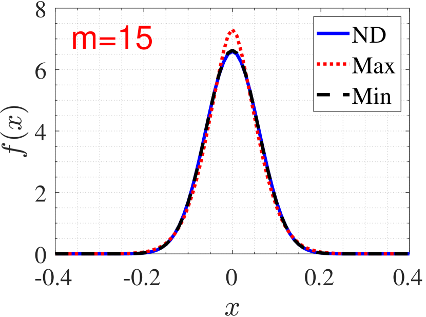
(b-1) Trevi:
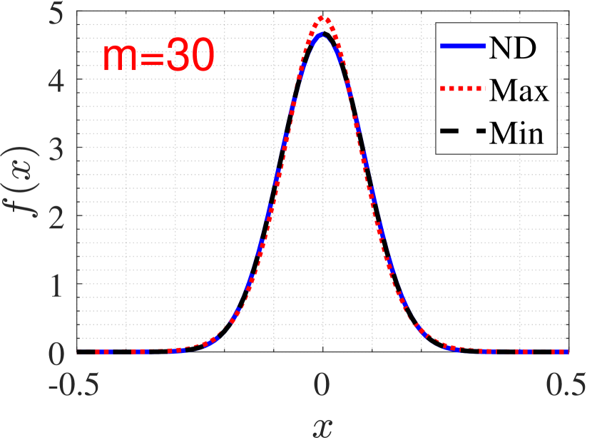
(b-2) Trevi:
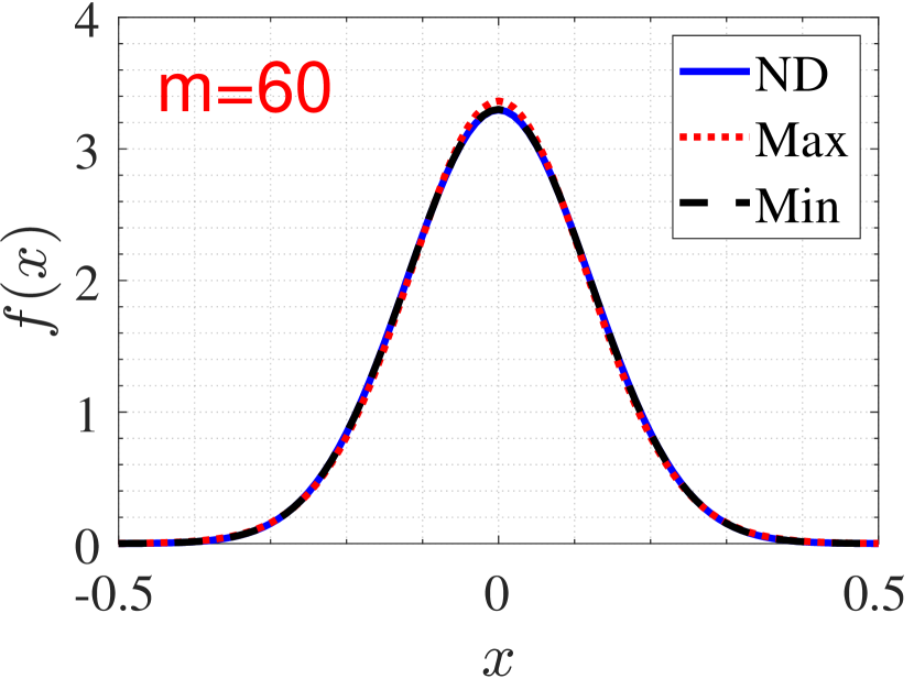
(b-3) Trevi:
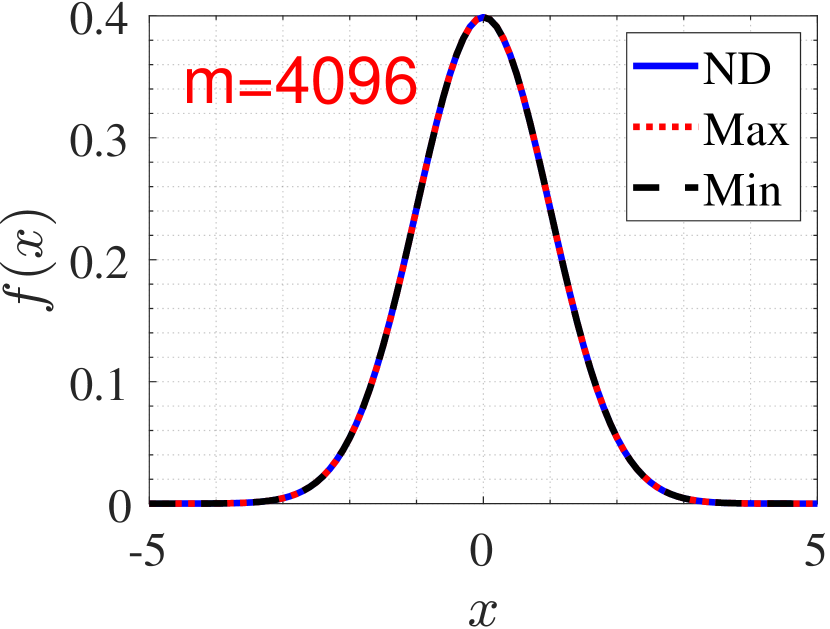
(b-4) Trevi:
Fact 4.9.
(Hoel et al., 1971) The first four moments of are:
It is easy to see that and are monotonously decreasing function of and increasing function of (). Hence, the first four moments of and are equal with each other, respectively, as approaches infinity. This is consistent with Corollary 4.7.
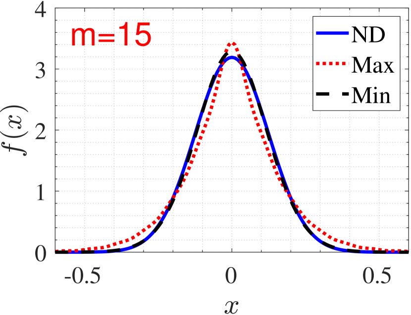
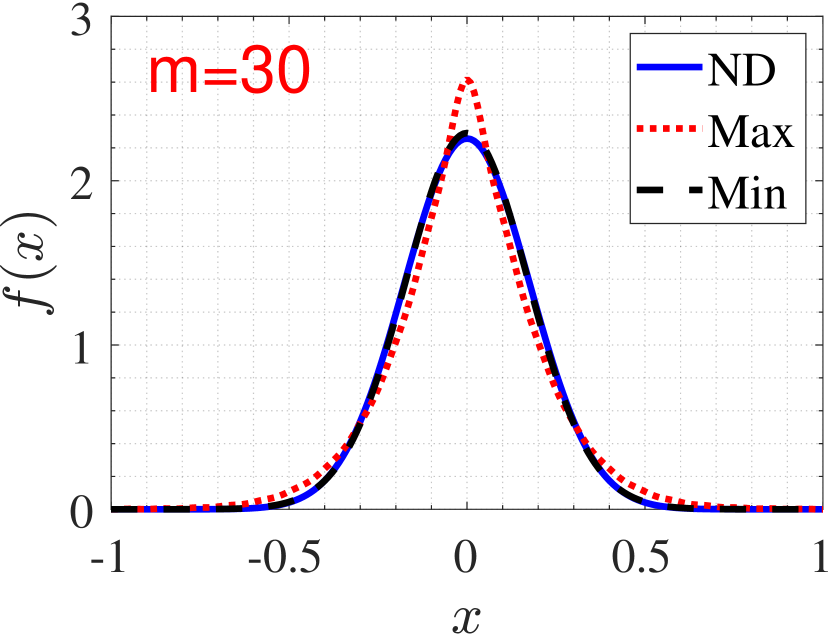
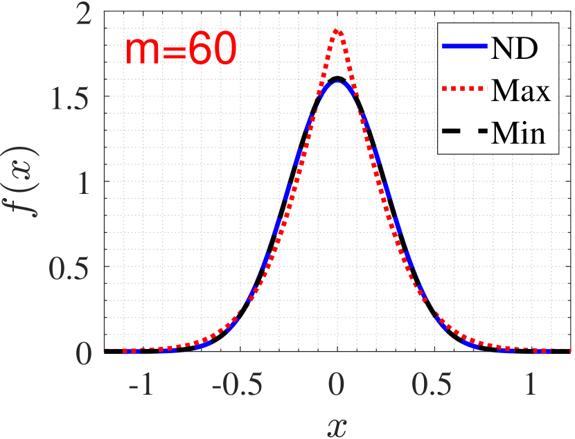
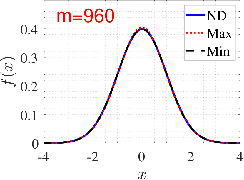
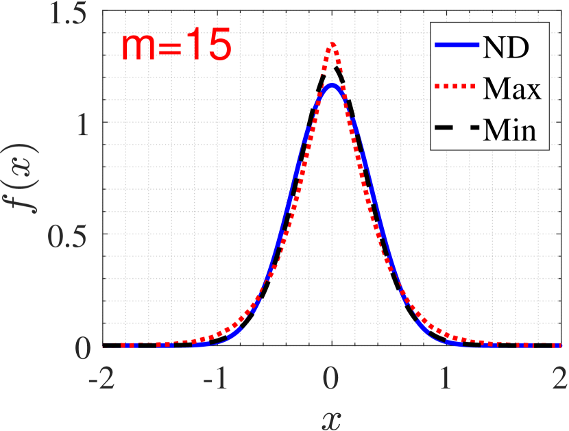
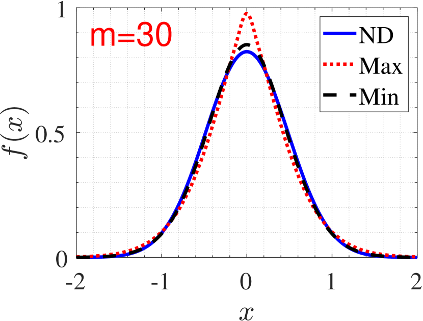
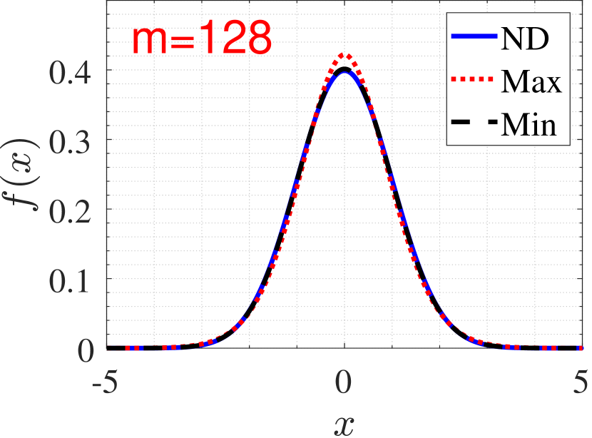
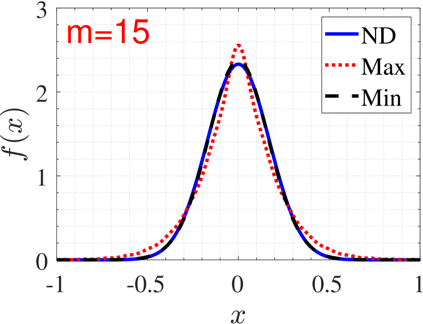
For limited , the impact of is not negligible. However, we can easily adjust to control the impact of (the data-dependent factor) on within a reasonable range. Table 2 in Appendix C lists the values of and for different over 12 datasets, where and are calculated using the maximum, mean and minimum , respectively. As expected, and decrease as increases. Take Trevi as an example, is equal to 0 and is very tiny (0.0001-0.000729) when , manifesting the equivalence between and the PDF of as depicted in Figure 1 (b-4). In the case of , it also suffices to provide small enough and , indicating the high similarity between the distribution of and .
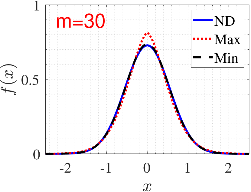
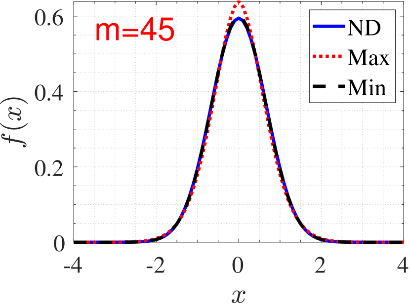
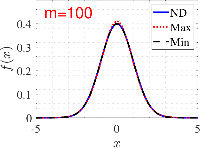
To visualize the similarity, we plot for different under the maximum and minimum , and the PDF of in Figure 1 for two datasets Gist and Trevi. More plots for other datasets are listed in Figure 4 in Appendix C. Three observations can be made from these figures: (1) the distribution of matches very well with for small ; (2) for large , differs only slightly from the PDF of for all , indicating that is the dominating factor in ; (3) greater results in higher similarity between and , implying that FastLSH can always achieve almost the same performance as E2LSH by choosing appropriately.
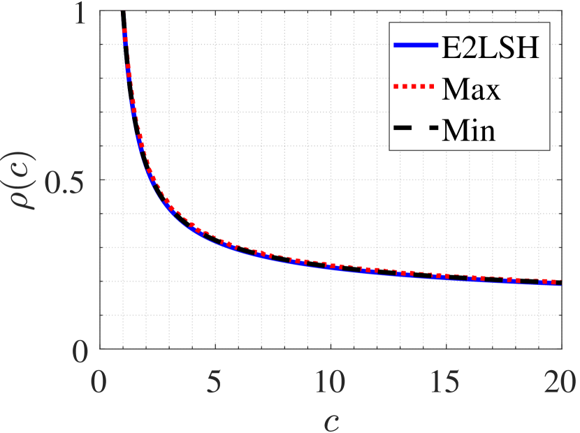
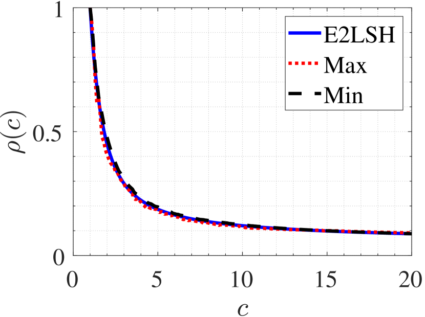
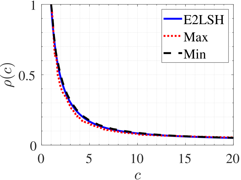
To further validate the LSH property of FastLSH, we compare the important parameter for FastLSH and E2LSH when . is defined as the function of the approximation ratio , i.e., , where and . Note that affects both the space and time efficiency of LSH algorithms. For in the range (with increments of 0.1), we calculate using Matlab, where the minimal and maximal are collected for different (). The plots of under different bucket widths over the datasets Gist and Trevi are illustrated in Figure 2. Clearly, the curve of FastLSH matches very well with that of E2LSH, verifying that FastLSH maintains almost the same LSH property with E2LSH even when is relatively small. More plots of for other datesets are given in Figure 5 and Figure 6 in Appendix C.
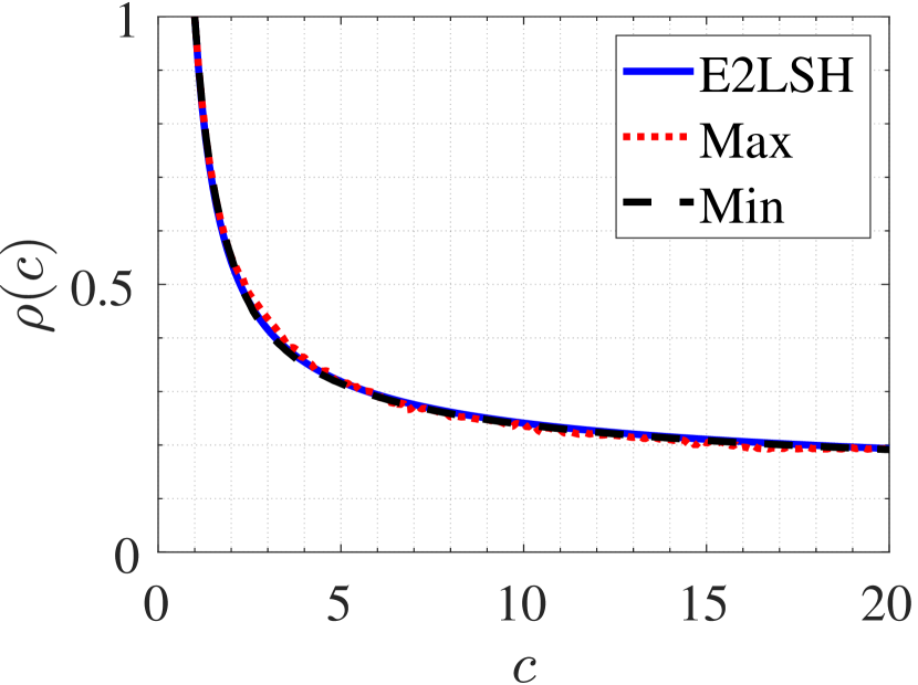
(a-1) Gist: = 0.255 and = 1.5

(a-2) Gist: = 0.73 and = 4
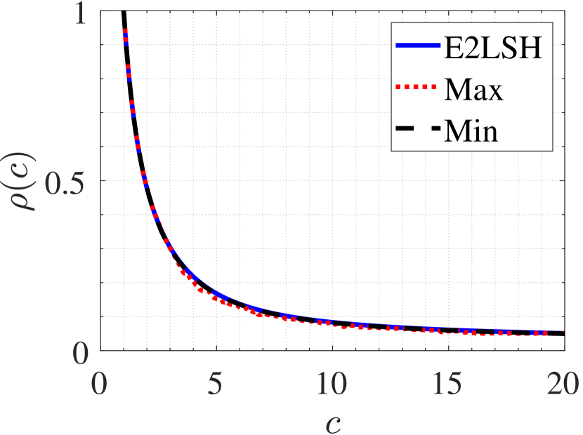
(a-3) Gist: = 1.8 and = 10

(b-1) Trevi: = 0.127 and = 1.5
(b-2) Trevi: = 0.35 and = 4

(b-3) Trevi: = 0.86 and = 10
5 Extension to Other Similarity Metrics
In this section, we sketch how to extend FastLSH to other similarity measures. Since the angular similarity can be well approximated by the Euclidean distance if the norms of data item are identical, one can use FastLSH for the angular similarity directly after data normalization. In addition, FastLSH can solve the maximum inner product search problem by utilizing two transformation functions (Bachrach et al., 2014). The detailed discussion is given in Appendix B. The extension of FastLSH to support norm for is left as our future work.
6 Experiments
In this section we evaluate the performance of FastLSH against other LSH algorithms for the ANN search task. All algorithms follow the standard hash table construction and search procedure as discussed in Section 3.2. All experiments are carried out on the server with six-cores Intel(R), i7-8750H @ 2.20GHz CPUs and 32 GB RAM, in Ubuntu 20.04.
Datasets: 11 publicly available high-dimensional real datasets and one synthetic dataset are experimented with (Li et al., 2019), the statistics of which are listed in Table 1. Sun 111http://groups.csail.mit.edu/vision/SUN/ is the set of containing about 70k GIST features of images. Cifar 222http://www.cs.toronto.edu/ kriz/cifar.html is denoted as the set of 50k vectors extracted from TinyImage. Audio 333http://www.cs.princeton.edu/cass/audio.tar.gz is the set of about 50k vectors extracted from DARPA TIMIT. Trevi 444http://phototour.cs.washington.edu/patches/default.htm is the set of containing around 100k features of bitmap images. Notre 555http://phototour.cs.washington.edu/datasets/ is the set of features that are Flickr images and a reconstruction. Sift 666http://corpus-texmex.irisa.fr is the set of containing 1 million SIFT vectors. Gist 777https://github.com/aaalgo/kgraph is the set that is consist of 1 million image vectors. Deep 888https://yadi.sk/d/I_yaFVqchJmoc is the set of 1 million vectors that are deep neural codes of natural images obtained by convolutional neural network. Ukbench 999http://vis.uky.edu/ stewe/ukbench/ is the set of vectors containing 1 million features of images. Glove 101010http://nlp.stanford.edu/projects/glove/ is the set of about 1.2 million feature vectors extracted from Tweets. ImageNet 111111http://cloudcv.org/objdetect/ is the set of data points containing about 2.4 million dense SIFT features. Random is the set containing 1 million randomly selected vectors in a unit hypersphere.
| Datasets | # of Points | # of Queries | Dimension |
|---|---|---|---|
| Sun | 69106 | 200 | 512 |
| Cifar | 50000 | 200 | 512 |
| Audio | 53387 | 200 | 192 |
| Trevi | 99000 | 200 | 4096 |
| Notre | 333000 | 200 | 128 |
| Sift | 1000000 | 200 | 128 |
| Gist | 1000000 | 200 | 960 |
| Deep | 1000000 | 200 | 256 |
| Ukbench | 1000000 | 200 | 128 |
| Glove | 1192514 | 200 | 100 |
| ImageNet | 2340000 | 200 | 150 |
| Random | 1000000 | 200 | 100 |
Baselines: We compare FastLSH with two popular LSH algorithms, i.e., E2LSH (Datar et al., 2004; Andoni, 2005) and ACHash (Dasgupta et al., 2011). E2LSH is the vanilla LSH scheme for approximate near neighbor search with sub-linear query time. ACHash is proposed to speedup the hash function evaluation by using Hadamard transform and sparse random projection. Note that ACHash is actually not an eligible LSH method because no expression of the probability of collision exists for ACHash, not mentioning the desirable LSH property. We choose ACHash as one of the baselines for the sake of completeness.
(a)
(b)
(c)
(d)
(e)
(f)
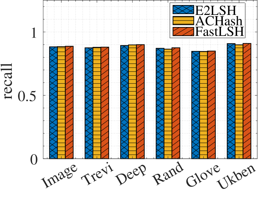
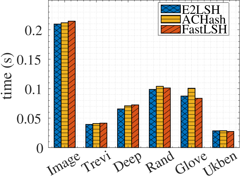
Evaluation Metrics: To evaluate the performance of FastLSH and baselines, we present the following metrics: 1) the average recall, i.e., the fraction of near neighbors that are actually returned; 2) the average running time to report the near neighbors for each query; 3) the time taken to compute hash functions.
Parameter Settings: For the same dataset and target recall, we use identical (number of hash functions per table) and (number of hash tables) for fairness. Thus, three algorithms take the same space occupations. is set to 30 throughout all experiments for FastLSH. To achieve optimal performance, the sampling ratio for ACHash is set to the defaulst 0.25. We report R10@10 over all of the datasets for three algorithms.
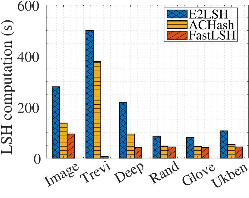
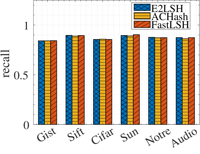
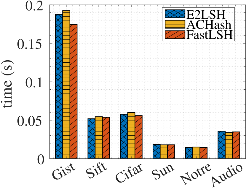
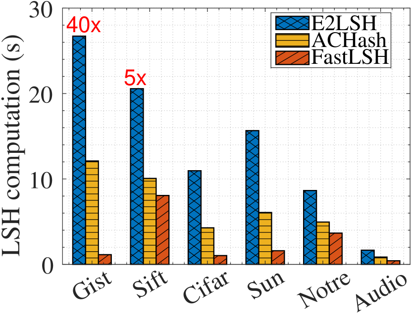
Experiment 1: In this set of experiments, we set the target recall as 0.9. By tuning , and bucket widths, the three methods achieve almost the same recall on the same dataset with the optimal query time 121212The actual recall may vary around 0.9 slightly. The recall, average query time and LSH computation time are illustrated in Figure 3 (a), (b), (d) and (e). As analyzed in Section 4.2, FastLSH and E2LSH owns similar theoretical property, and thus achieve comparable query performance and answer accuracy as plotted in Figure 3. Due to lack of theoretical guarantee, ACHash performs slightly worse than FastLSH and E2LSH in most cases w.r.t query efficiency.
The performance of the three methods differs dramatically when it turns to the cost of hashing. As shown in Figure 3 (c) and (f), the LSH computation time of FastLSH is significantly superior to E2LSH and ACHash. For example, FastLSH obtains around 80 speedup over E2LSH and runs 60 times faster than ACHash on Trevi. This is because the time complexity of FastLSH is only instead of of E2LSH. For ACHash, the fixed sampling ratio and overhead in Hadamard transform make it inferior to FastLSH.
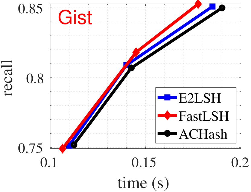
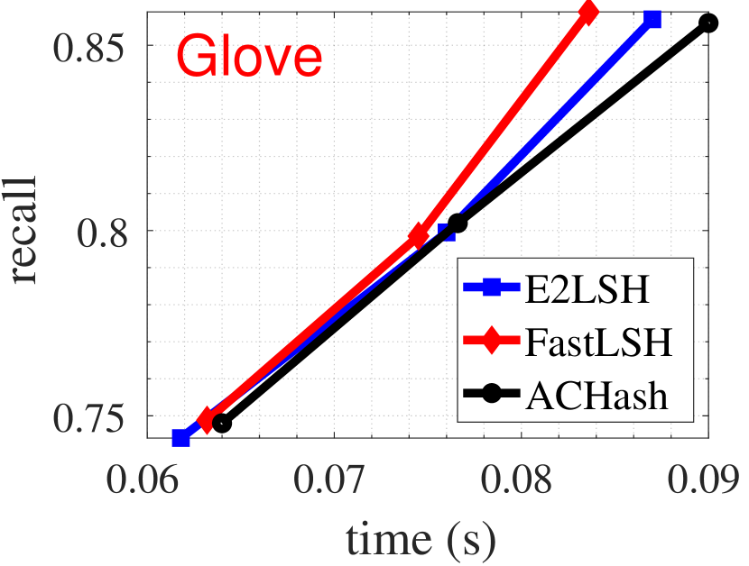
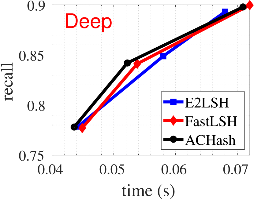
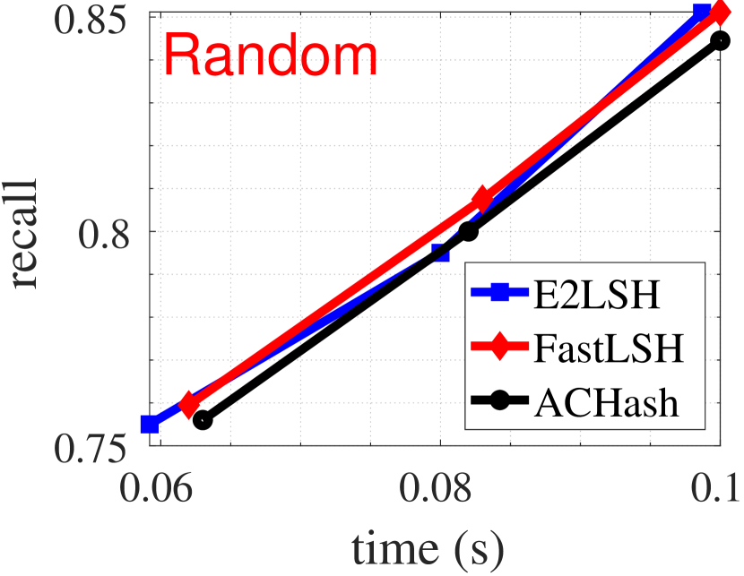
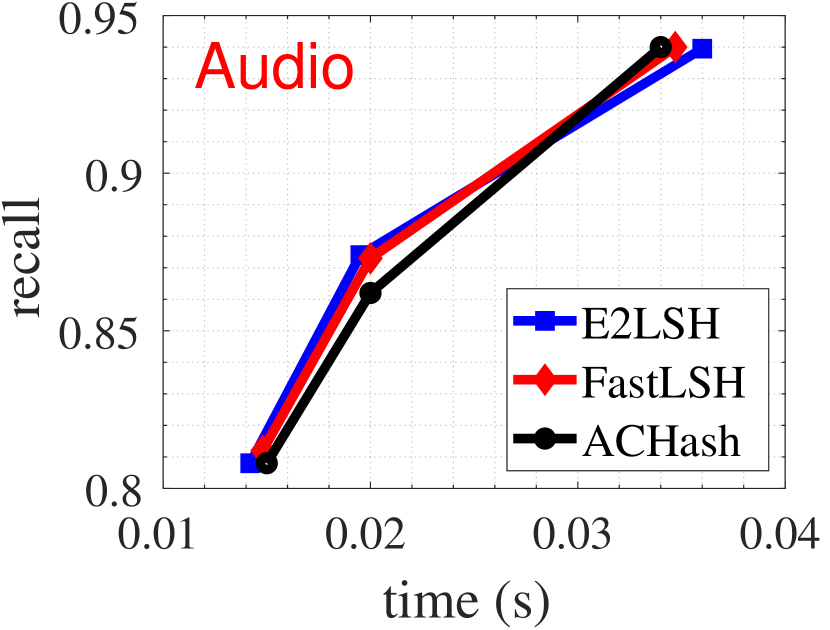
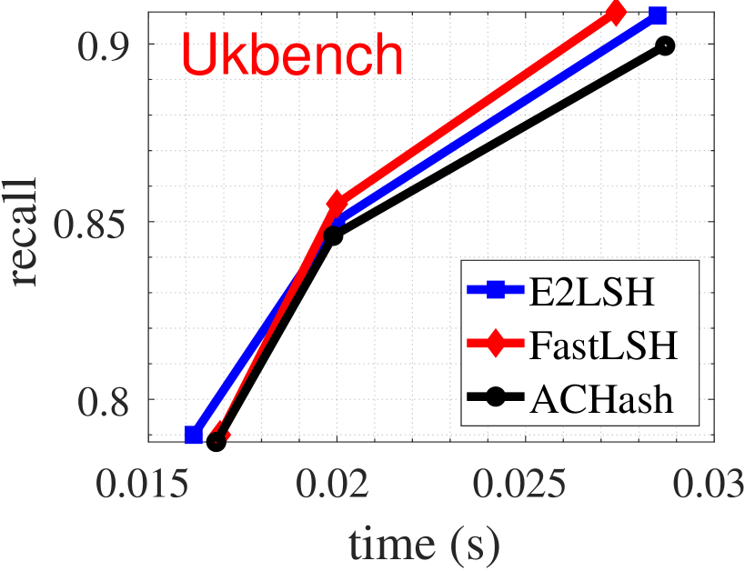
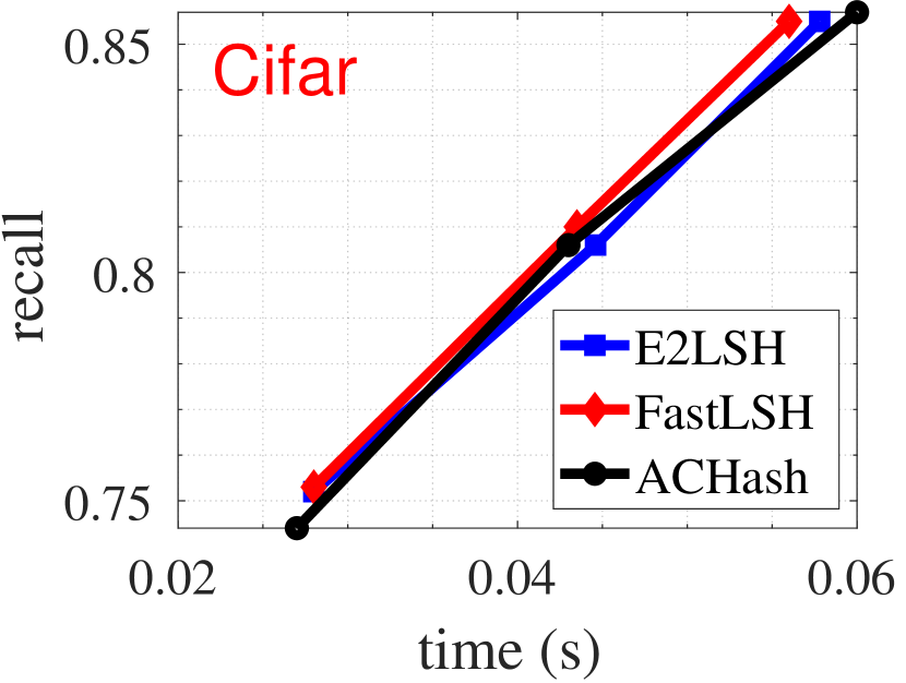
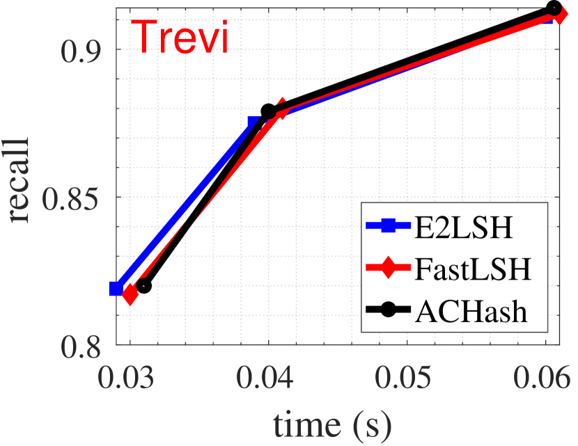
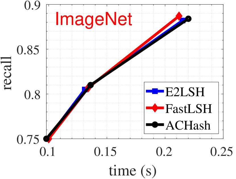
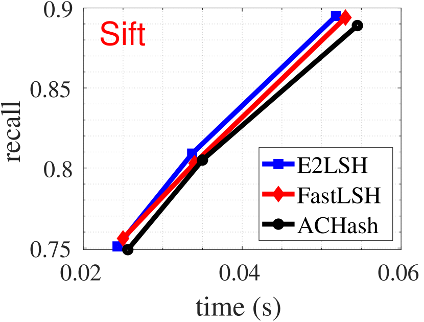
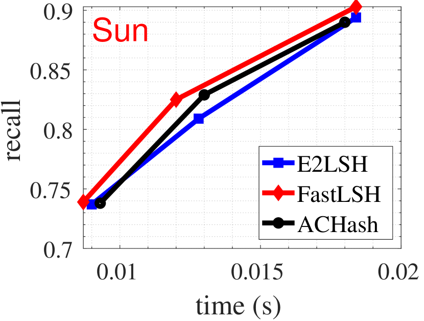
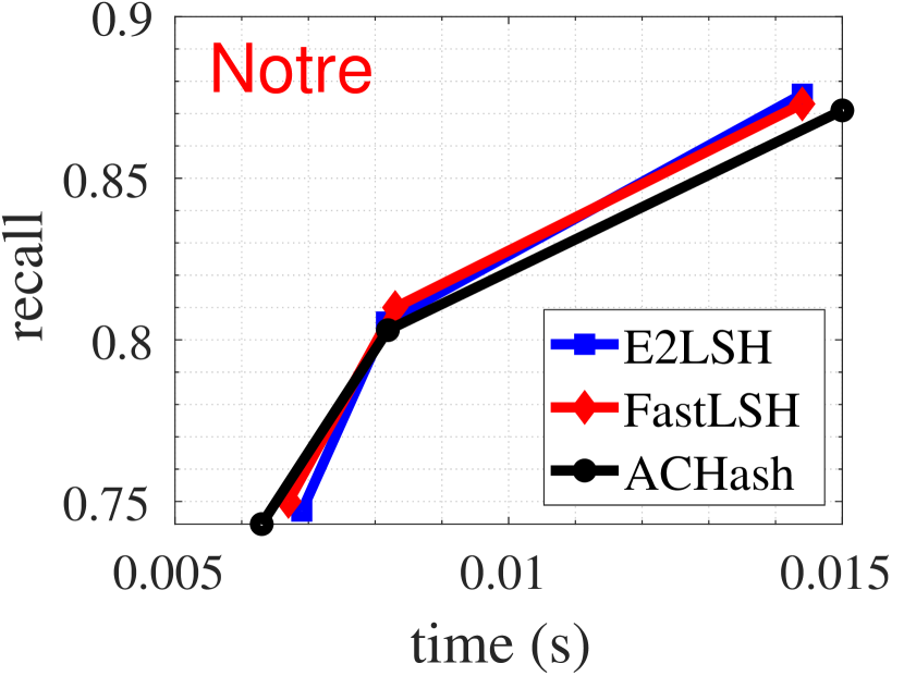
Experiment 2: We also plot the recall v.s. average query time curves by varying target recalls to obtain a complete picture of FastLSH, which are depicted in Figure 7 in Appendix C due to space limitation. The empirical results demonstrate that FastLSH performs almost the same in terms of answer accuracy, query efficiency and space occupation as E2LSH. This further validates that FastLSH owns the same LSH property as E2LSH with limited . Again, ACHash is slightly inferior to the others in most cases.
In sum, FastLSH is on par with E2LSH (with provable LSH property) in terms of answer accuracy and query efficiency and marginally superior to ACHash (without provable LSH property), while significantly reducing the cost of hashing. We believe that FastLSH is a promising alternative to the existing hashing schemes for norm.
7 Conclusion
In this paper, we develop FastLSH to accelerate hash function evaluation, which maintains the same theoretical guarantee and empirical performance as the classic E2LSH. Rigid analysis shows that the probability of collision of FastLSH is asymptotically equal to that of E2LSH. In the case of limited , we quantitatively analyze the impact of and on the probability of collision. Extensive experiments on a number of datasets demonstrate that FastLSH is a promising alternative to the classic LSH scheme.
References
- Ailon & Chazelle (2006) Ailon, N. and Chazelle, B. Approximate nearest neighbors and the fast johnson-lindenstrauss transform. In Proceedings of the thirty-eighth annual ACM symposium on Theory of computing, pp. 557–563, 2006.
- Ailon & Liberty (2009) Ailon, N. and Liberty, E. Fast dimension reduction using rademacher series on dual bch codes. Discrete & Computational Geometry, 42:615–630, 2009.
- Andoni (2005) Andoni, A. E2lsh-0.1 user manual. http://web.mit.edu/andoni/www/LSH/index.html, 2005.
- Andoni & Indyk (2008) Andoni, A. and Indyk, P. Near-optimal hashing algorithms for approximate nearest neighbor in high dimensions. Communications of the ACM, 51(1):117–122, 2008.
- Bachrach et al. (2014) Bachrach, Y., Finkelstein, Y., Gilad-Bachrach, R., Katzir, L., Koenigstein, N., Nice, N., and Paquet, U. Speeding up the xbox recommender system using a euclidean transformation for inner-product spaces. In Proceedings of the 8th ACM Conference on Recommender systems, pp. 257–264, 2014.
- Bentley (1975) Bentley, J. L. Multidimensional binary search trees used for associative searching. Communications of the ACM, 18(9):509–517, 1975.
- Charikar (2002) Charikar, M. S. Similarity estimation techniques from rounding algorithms. In Proceedings of the thiry-fourth annual ACM symposium on Theory of computing, pp. 380–388, 2002.
- Chen et al. (2020) Chen, B., Medini, T., Farwell, J., Tai, C., Shrivastava, A., et al. Slide: In defense of smart algorithms over hardware acceleration for large-scale deep learning systems. Proceedings of Machine Learning and Systems, 2:291–306, 2020.
- Chen et al. (2011) Chen, C., Horng, S.-J., and Huang, C.-P. Locality sensitive hashing for sampling-based algorithms in association rule mining. Expert Systems with Applications, 38(10):12388–12397, 2011.
- Cohen (1991) Cohen, A. C. Truncated and censored samples: theory and applications. CRC press, 1991.
- Dasgupta et al. (2011) Dasgupta, A., Kumar, R., and Sarlós, T. Fast locality-sensitive hashing. In Proceedings of the 17th ACM SIGKDD international conference on Knowledge discovery and data mining, pp. 1073–1081, 2011.
- Datar et al. (2004) Datar, M., Immorlica, N., Indyk, P., and Mirrokni, V. S. Locality-sensitive hashing scheme based on p-stable distributions. In Proceedings of the twentieth annual symposium on Computational geometry, pp. 253–262, 2004.
- Feller (1991) Feller, W. An introduction to probability theory and its applications, Volume 2, volume 81. John Wiley & Sons, 1991.
- Gan et al. (2012) Gan, J., Feng, J., Fang, Q., and Ng, W. Locality-sensitive hashing scheme based on dynamic collision counting. In Proceedings of the 2012 ACM SIGMOD international conference on management of data, pp. 541–552, 2012.
- Hoel et al. (1971) Hoel, P. G., Port, S. C., and Stone, C. J. Introduction to probability theory. Houghtion Mifflin, 1971.
- Huang et al. (2015) Huang, Q., Feng, J., Zhang, Y., Fang, Q., and Ng, W. Query-aware locality-sensitive hashing for approximate nearest neighbor search. Proceedings of the VLDB Endowment, 9(1):1–12, 2015.
- Indyk & Motwani (1998) Indyk, P. and Motwani, R. Approximate nearest neighbors: towards removing the curse of dimensionality. In Proceedings of the thirtieth annual ACM symposium on Theory of computing, pp. 604–613, 1998.
- Islam (2018) Islam, M. R. Sample size and its role in central limit theorem (clt). International Journal of Physics and Mathematics, 1(1):37–47, 7 2018.
- Johnson (1949) Johnson, N. L. Systems of frequency curves generated by methods of translation. Biometrika, 36(1/2):149–176, 1949.
- Katayama & Satoh (1997) Katayama, N. and Satoh, S. The sr-tree: An index structure for high-dimensional nearest neighbor queries. ACM Sigmod Record, 26(2):369–380, 1997.
- Koga et al. (2007) Koga, H., Ishibashi, T., and Watanabe, T. Fast agglomerative hierarchical clustering algorithm using locality-sensitive hashing. Knowledge and Information Systems, 12:25–53, 2007.
- Kushilevitz et al. (1998) Kushilevitz, E., Ostrovsky, R., and Rabani, Y. Efficient search for approximate nearest neighbor in high dimensional spaces. In Proceedings of the thirtieth annual ACM symposium on Theory of computing, pp. 614–623, 1998.
- Leslie (1959) Leslie, D. Determination of parameters in the johnson system of probability distributions. Biometrika, 46(1/2):229–231, 1959.
- Li et al. (2019) Li, W., Zhang, Y., Sun, Y., Wang, W., Li, M., Zhang, W., and Lin, X. Approximate nearest neighbor search on high dimensional data—experiments, analyses, and improvement. IEEE Transactions on Knowledge and Data Engineering, 32(8):1475–1488, 2019.
- Lin (2017) Lin, G. D. Recent developments on the moment problem. Journal of Statistical Distributions and Applications, 4(1):5, 2017.
- Lu & Kudo (2020) Lu, K. and Kudo, M. R2lsh: A nearest neighbor search scheme based on two-dimensional projected spaces. In 2020 IEEE 36th International Conference on Data Engineering (ICDE), pp. 1045–1056. IEEE, 2020.
- Lv et al. (2007) Lv, Q., Josephson, W., Wang, Z., Charikar, M., and Li, K. Multi-probe lsh: efficient indexing for high-dimensional similarity search. In Proceedings of the 33rd international conference on Very large data bases, pp. 950–961, 2007.
- Ramberg et al. (1979) Ramberg, J. S., Dudewicz, E. J., Tadikamalla, P. R., and Mykytka, E. F. A probability distribution and its uses in fitting data. Technometrics, 21(2):201–214, 1979.
- Samet (2006) Samet, H. Foundations of multidimensional and metric data structures. Morgan Kaufmann, 2006.
- Shrivastava (2017) Shrivastava, A. Optimal densification for fast and accurate minwise hashing. In International Conference on Machine Learning, pp. 3154–3163. PMLR, 2017.
- Shrivastava & Li (2014a) Shrivastava, A. and Li, P. Asymmetric lsh (alsh) for sublinear time maximum inner product search (mips). Advances in neural information processing systems, 27:2321–2329, 2014a.
- Shrivastava & Li (2014b) Shrivastava, A. and Li, P. Densifying one permutation hashing via rotation for fast near neighbor search. In International Conference on Machine Learning, pp. 557–565. PMLR, 2014b.
- Sun et al. (2014) Sun, Y., Wang, W., Qin, J., Zhang, Y., and Lin, X. Srs: solving c-approximate nearest neighbor queries in high dimensional euclidean space with a tiny index. Proceedings of the VLDB Endowment, 2014.
- Sundaram et al. (2013) Sundaram, N., Turmukhametova, A., Satish, N., Mostak, T., Indyk, P., Madden, S., and Dubey, P. Streaming similarity search over one billion tweets using parallel locality-sensitive hashing. Proceedings of the VLDB Endowment, 6(14):1930–1941, 2013.
- Tao et al. (2010) Tao, Y., Yi, K., Sheng, C., and Kalnis, P. Efficient and accurate nearest neighbor and closest pair search in high-dimensional space. ACM Transactions on Database Systems (TODS), 35(3):1–46, 2010.
- Tian et al. (2022) Tian, Y., Zhao, X., and Zhou, X. Db-lsh: Locality-sensitive hashing with query-based dynamic bucketing. In 2022 IEEE 38th International Conference on Data Engineering (ICDE), pp. 2250–2262. IEEE, 2022.
- Yang et al. (2020) Yang, C., Deng, D., Shang, S., and Shao, L. Efficient locality-sensitive hashing over high-dimensional data streams. In 2020 IEEE 36th International Conference on Data Engineering (ICDE), pp. 1986–1989. IEEE, 2020.
- Zheng et al. (2020) Zheng, B., Xi, Z., Weng, L., Hung, N. Q. V., Liu, H., and Jensen, C. S. Pm-lsh: A fast and accurate lsh framework for high-dimensional approximate nn search. Proceedings of the VLDB Endowment, 13(5):643–655, 2020.
- Zolotarev (1986) Zolotarev, V. M. One-dimensional stable distributions, volume 65 of Translations of Mathematical Monographs. American Mathematical Society, 1986.
Appendix
Appendix A Proofs
Lemma A.1.
The characteristic function of the product of two independent random variables is as follows:
where is a standard normal random variable and is an independent random variable with mean and variance .
Proof.
For the characteristic function of , we can write:
where standard normal random variable is eliminated by its characteristic function. We prove this Lemma. ∎
Lemma A.2.
The characteristic function of is as follows:
where is the complementary error function.
Proof.
Theorem A.3.
The collision probability of FastLSH is as follows:
Proof.
Let represent the PDF of the absolute value of . For given bucket width , the probability for any pair is computed as , where . Recall that follows the uniform distribution , the probability is thus . This means that after random projection, is also within the same bucket, and the collision probability is the product of and . Hence we prove this Theorem. ∎
Theorem A.4.
where and is the characteristic function of .
Proof.
Recall that and . can be written as follows:
Let and . According to the fact , is simplified as:
Let , where is the characteristic function of . Then is denoted as:
To prove , we convert to prove whether as . Obviously . Then and . It is easy to derive:
It holds for any fixed . On the other hand, we have:
Actually using the fact as and as , we have:
Hence we have:
∎
If the characteristic function of a random variable exists, it provides a way to compute its various moments. Specifically, the -th moment of denoted by can be expressed as the -th derivative of the characteristic function evaluated at zero (Hoel et al., 1971), i.e.,
| (10) |
where denotes the characteristic function of . If we know the characteristic function, then all of the moments of the random variable can be obtained.
Lemma A.5.
where and .
Proof.
From Lemma A.2, we can easily compute the first-order derivative of characteristic function with respect to , which is as follows:
| (11) |
Then the second-order derivative is
| (12) | ||||
The third-order derivative is
| (13) | ||||
The fourth-order derivative is
| (14) | ||||
Let for denote the first four central moments. According to Eqn. (10), we know that , then it is easy to derive . To this end, by Eqn. (11) - (14), we have the following results:
| (15) |
where is the expectation; is the variance; is the skewness; is the kurtosis. Since
Therefore, Eqn. (15) can be rewritten as below
where , , and . We prove this Lemma.
∎
Appendix B Extension to Maximum Inner Product Search
(Bachrach et al., 2014; Shrivastava & Li, 2014a) shows that there exists two transformation functions, by which the maximum inner product search (MIPS) problem can be converted into solve the near neighbor search problem. More specifically, the two transformation functions are for data processing and for query processing respectively, where . Then the relationship between maximum inner product and norm for any vector pair is denoted as for . To make FastLSH applicable for MIPS, we first apply the sample operator defined earlier to vector pairs for yielding and , and then obtain and , where is a constant. Then for . Let . After random projection, is distributed as . Since , then . Let be the random variable . Similar to Eqn. (7), the PDF of represented by is yielded as follow:
| (16) |
By applying Lemma A.1, the characteristic function of is as follows:
| (17) |
Then the PDF of is obtained by :
| (18) |
It is easy to derive the collision probability of any pair by , which is as follows:
| (19) |
where denotes the PDF of the absolute value of . is the bucket width.
Appendix C Additional Experiments
| Datasets | |||||||||
| Cifar | max | 0.567575 | 2.527575 | 0.287600 | 1.287600 | 0.114125 | 0.618225 | 0.000064 | 0.067664 |
| mean | 0.102716 | 0.575372 | 0.027539 | 0.277239 | 0.001994 | 0.120123 | 0 | 0.014617 | |
| min | 0.019616 | 0.239671 | 0.001702 | 0.116014 | 0.000011 | 0.055001 | 0 | 0.006691 | |
| Sun | max | 0.502360 | 2.218460 | 0.236626 | 1.084867 | 0.095099 | 0.546683 | 0.000006 | 0.051535 |
| mean | 0.022783 | 0.255107 | 0.001849 | 0.118130 | 0.000018 | 0.058099 | 0 | 0.006724 | |
| min | 0 | 0.040401 | 0 | 0.020736 | 0 | 0.010000 | 0 | 0.001156 | |
| Gist | max | 0.633640 | 2.853740 | 0.274502 | 1.234902 | 0.129940 | 0.677540 | 0 | 0.032400 |
| mean | 0.042122 | 0.340238 | 0.005183 | 0.152639 | 0.000133 | 0.074662 | 0 | 0.004624 | |
| min | 0.000064 | 0.067664 | 0 | 0.038025 | 0 | 0.016926 | 0 | 0.001089 | |
| Trevi | max | 0.013420 | 0.207020 | 0.001105 | 0.106081 | 0.000003 | 0.049287 | 0 | 0.000729 |
| mean | 0.000011 | 0.055236 | 0 | 0.029241 | 0 | 0.013924 | 0 | 0.000196 | |
| min | 0 | 0.015876 | 0 | 0.008100 | 0 | 0.003969 | 0 | 0.000100 | |
| Audio | max | 0.268000 | 1.208900 | 0.099004 | 0.561404 | 0.043520 | 0.346020 | 0.000033 | 0.062533 |
| mean | 0.033344 | 0.303017 | 0.003637 | 0.138767 | 0.000480 | 0.091021 | 0 | 0.020967 | |
| min | 0.000022 | 0.059705 | 0 | 0.030765 | 0 | 0.021874 | 0 | 0.005329 | |
| Notre | max | 0.341109 | 1.507509 | 0.143598 | 0.728823 | 0.074226 | 0.467355 | 0.004017 | 0.142401 |
| mean | 0.022783 | 0.255107 | 0.001902 | 0.118866 | 0.000172 | 0.077456 | 0 | 0.027225 | |
| min | 0.000101 | 0.071925 | 0 | 0.036481 | 0 | 0.023716 | 0 | 0.008281 | |
| Glove | max | 0.261530 | 1.183130 | 0.094131 | 0.543031 | 0.040065 | 0.331665 | 0.002362 | 0.124862 |
| mean | 0.003190 | 0.134234 | 0.000047 | 0.065072 | 0.000001 | 0.043265 | 0 | 0.019853 | |
| min | 0.000025 | 0.060541 | 0 | 0.029929 | 0 | 0.020335 | 0 | 0.009409 | |
| Sift | max | 0.294194 | 1.314294 | 0.098513 | 0.559554 | 0.057014 | 0.400410 | 0.001296 | 0.109537 |
| mean | 0.054265 | 0.389506 | 0.007185 | 0.167986 | 0.001509 | 0.113065 | 0 | 0.036864 | |
| min | 0.003755 | 0.139916 | 0.000107 | 0.072468 | 0.000001 | 0.045370 | 0 | 0.016129 | |
| Deep | max | 0.036744 | 0.317644 | 0.003841 | 0.140741 | 0.000463 | 0.090463 | 0 | 0.014400 |
| mean | 0.003047 | 0.132719 | 0.000044 | 0.064560 | 0.000001 | 0.043306 | 0 | 0.007569 | |
| min | 0.000199 | 0.079160 | 0 | 0.039204 | 0 | 0.026374 | 0 | 0.004638 | |
| Random | max | 0.077344 | 0.479300 | 0.015195 | 0.216796 | 0.003505 | 0.137461 | 0.000041 | 0.064050 |
| mean | 0.002824 | 0.130273 | 0.000038 | 0.063542 | 0.000001 | 0.042437 | 0 | 0.019044 | |
| min | 0.000024 | 0.060049 | 0 | 0.029929 | 0. | 0.019881 | 0 | 0.008649 | |
| Ukbench | max | 0.692955 | 3.157855 | 0.361581 | 1.593681 | 0.217238 | 1.009338 | 0.039727 | 0.330248 |
| mean | 0.139183 | 0.712232 | 0.034502 | 0.308031 | 0.012672 | 0.202768 | 0.000056 | 0.066620 | |
| min | 0.002895 | 0.131059 | 0.000041 | 0.064050 | 0.000001 | 0.042437 | 0 | 0.015376 | |
| ImageNet | max | 0.466568 | 2.054168 | 0.217238 | 1.009338 | 0.119323 | 0.637723 | 0.004773 | 0.149173 |
| mean | 0.019125 | 0.237214 | 0.001336 | 0.110236 | 0.000107 | 0.072468 | 0 | 0.022201 | |
| min | 0 | 0.033489 | 0 | 0.016641 | 0 | 0.011025 | 0 | 0.003481 | |
![[Uncaptioned image]](/html/2309.15479/assets/x21.png)
(a-1) Audio:
![[Uncaptioned image]](/html/2309.15479/assets/x22.png)
(a-2) Audio:
![[Uncaptioned image]](/html/2309.15479/assets/x23.png)
(a-3) Audio:
![[Uncaptioned image]](/html/2309.15479/assets/x24.png)
(a-4) Audio:
![[Uncaptioned image]](/html/2309.15479/assets/x25.png)
(b-1) Cifar:
![[Uncaptioned image]](/html/2309.15479/assets/x26.png)
(b-2) Cifar:
![[Uncaptioned image]](/html/2309.15479/assets/x27.png)
(b-3) Cifar:
![[Uncaptioned image]](/html/2309.15479/assets/x28.png)
(b-4) Cifar:
![[Uncaptioned image]](/html/2309.15479/assets/x29.png)
(c-1) Deep:
![[Uncaptioned image]](/html/2309.15479/assets/x30.png)
(c-2) Deep:
![[Uncaptioned image]](/html/2309.15479/assets/x31.png)
(c-3) Deep:
![[Uncaptioned image]](/html/2309.15479/assets/x32.png)
(c-4) Deep:
![[Uncaptioned image]](/html/2309.15479/assets/x33.png)
(d-1) Glove:
![[Uncaptioned image]](/html/2309.15479/assets/x34.png)
(d-2) Glove:
![[Uncaptioned image]](/html/2309.15479/assets/x35.png)
(d-3) Glove:
![[Uncaptioned image]](/html/2309.15479/assets/x36.png)
(d-4) Glove:
![[Uncaptioned image]](/html/2309.15479/assets/x37.png)
(e-1) ImageNet:
![[Uncaptioned image]](/html/2309.15479/assets/x38.png)
(e-2) ImageNet:
![[Uncaptioned image]](/html/2309.15479/assets/x39.png)
(e-3) ImageNet:
![[Uncaptioned image]](/html/2309.15479/assets/x40.png)
(e-4) ImageNet:
![[Uncaptioned image]](/html/2309.15479/assets/x41.png)
(f-1) Notre:
![[Uncaptioned image]](/html/2309.15479/assets/x42.png)
(f-2) Notre:
![[Uncaptioned image]](/html/2309.15479/assets/x43.png)
(f-3) Notre:
![[Uncaptioned image]](/html/2309.15479/assets/x44.png)
(f-4) Notre:
(g-1) Sift:
(g-2) Sift:

(g-3) Sift:
(g-4) Sift:
(h-1) Sun:
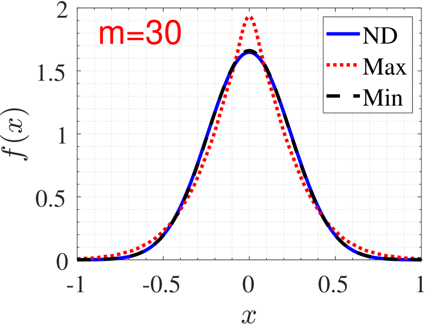
(h-2) Sun:
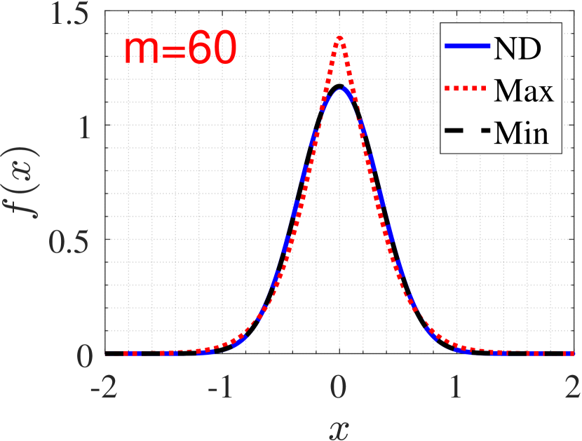
(h-3) Sun:
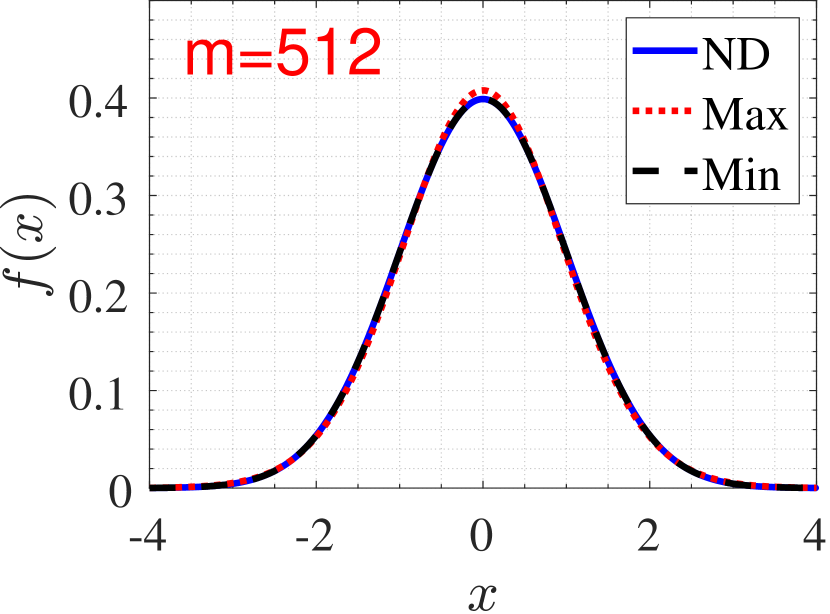
(h-4) Sun:
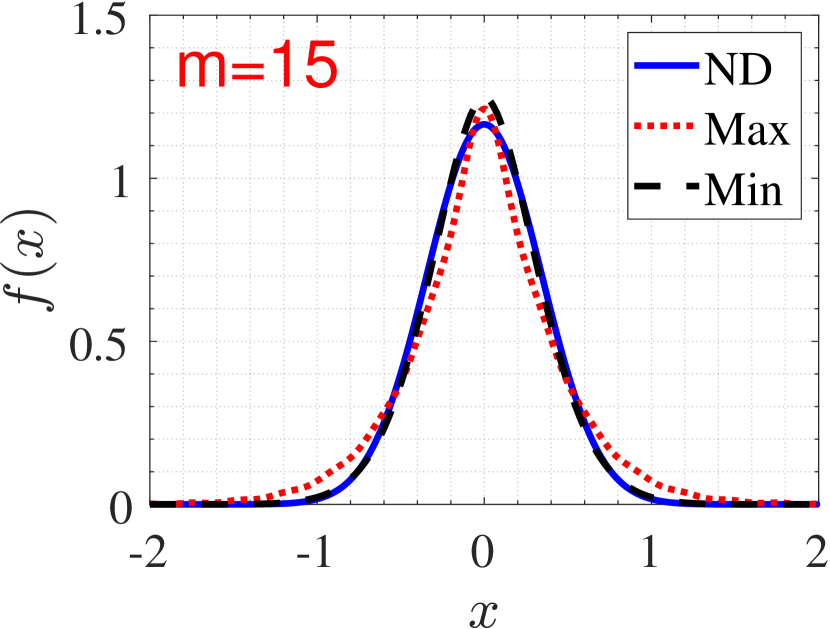
(i-1) Ukbench:
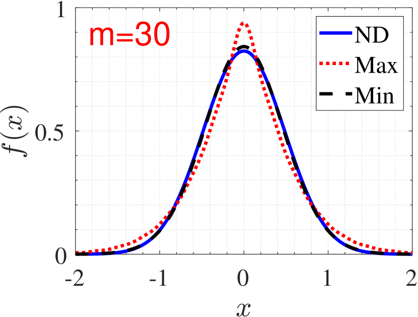
(i-2) Ukbench:
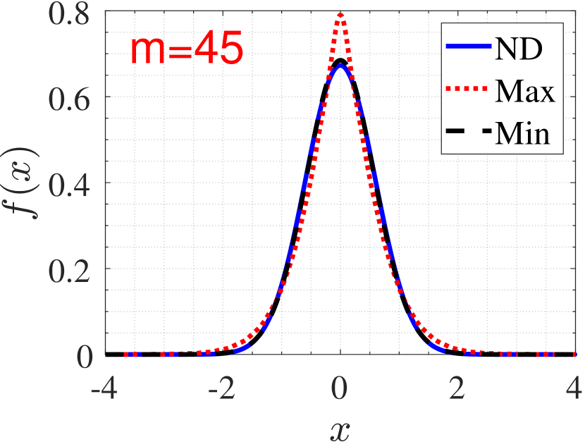
(i-3) Ukbench:
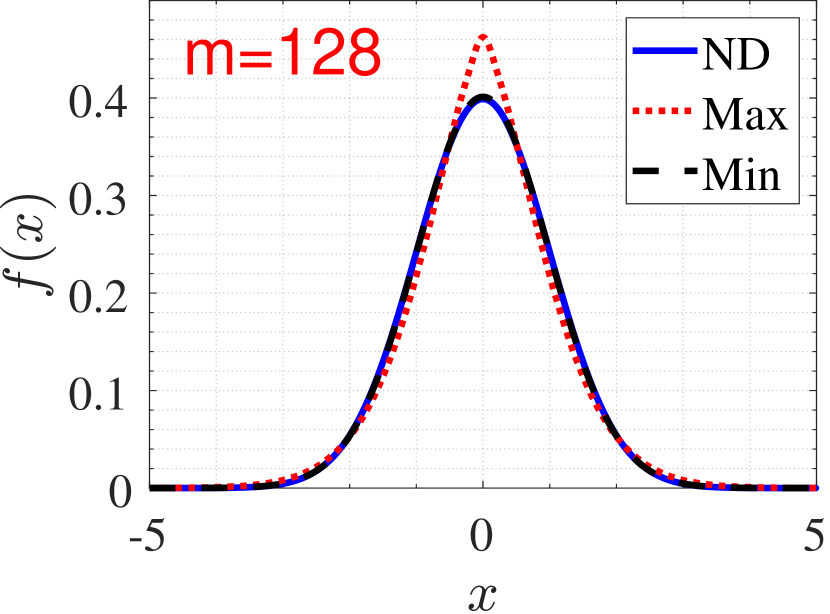
(i-4) Ukbench:
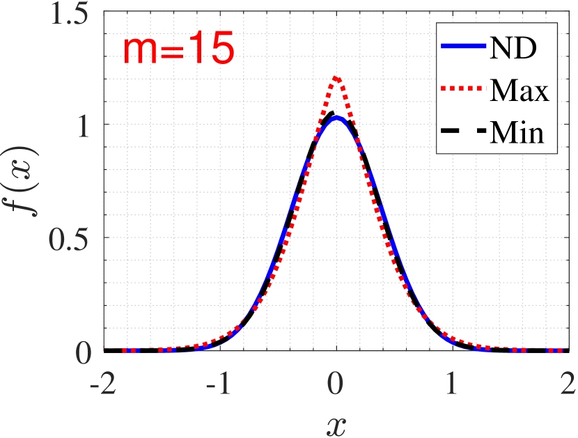
(j-1) Random:
(j-2) Random:
(j-3) Random:
(j-4) Random:
(a-1) Random: = 0.7 and = 1.5
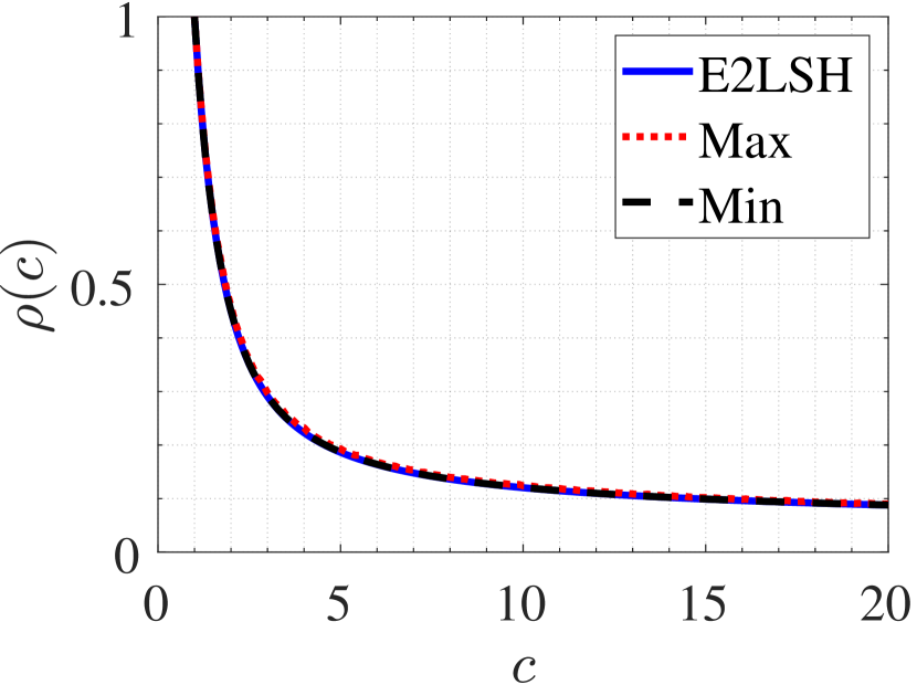
(a-2) Random: = 2 and = 4
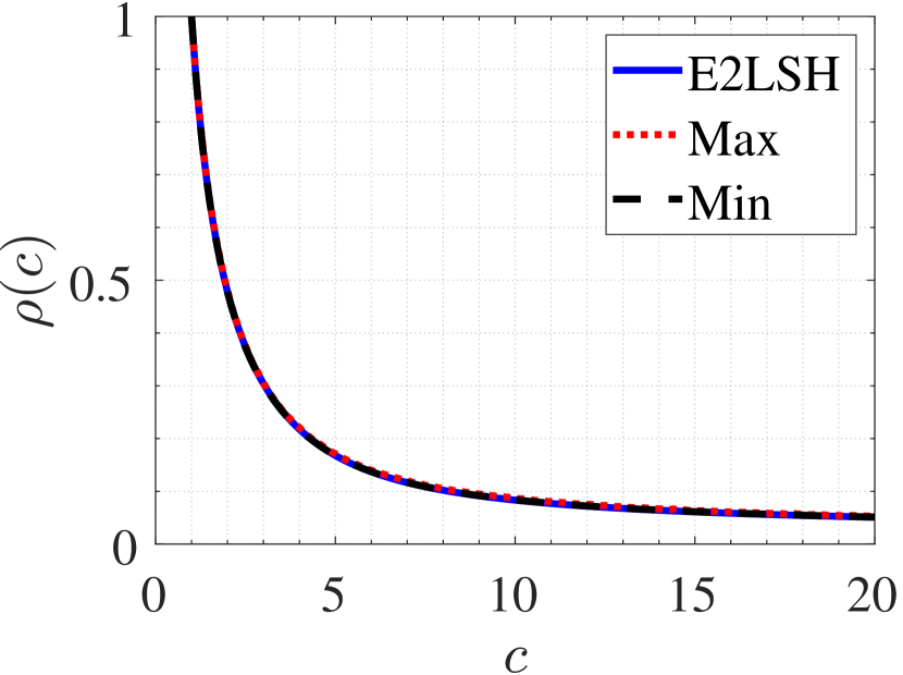
(a-3) Random: = 4.95 and = 10
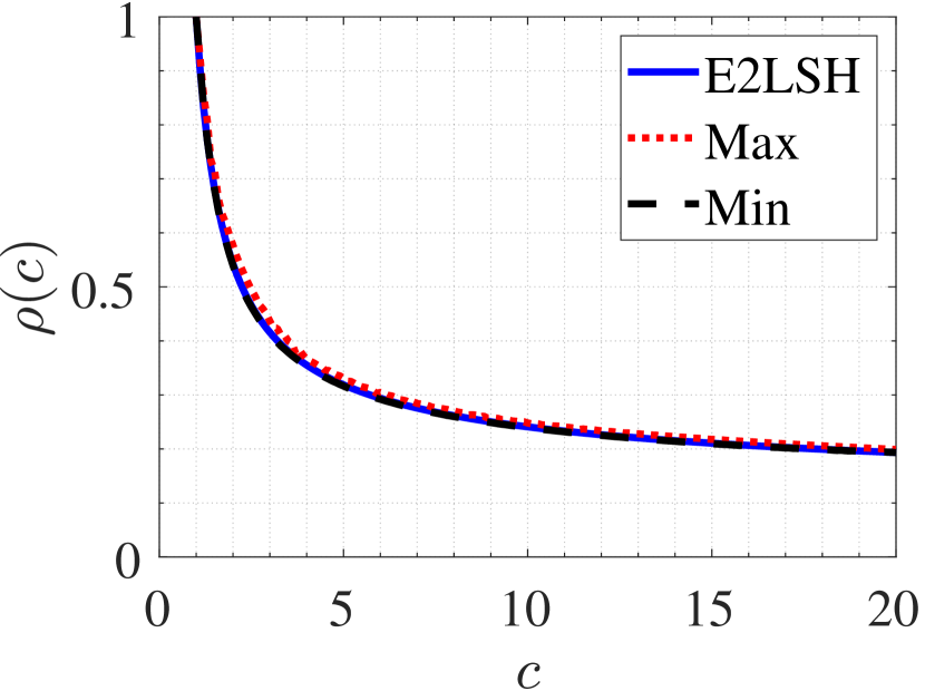
(b-1) Audio: = 0.59 and = 1.5

(b-2) Audio: = 1.6 and = 4

(b-3) Audio: = 3.95 and = 10
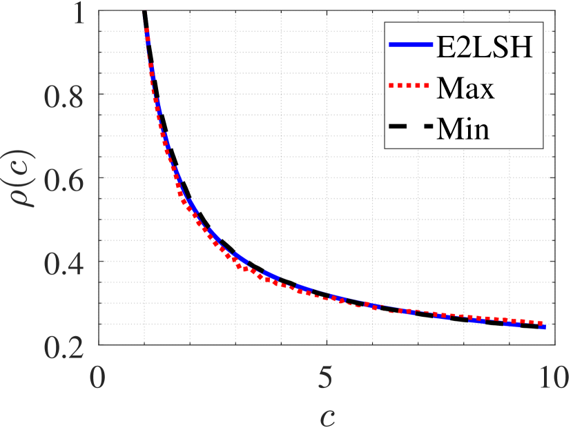
(c-1) Cifar: = 0.345 and = 1.5
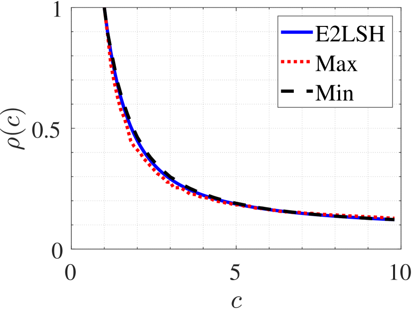
(c-2) Cifar: = 1 and = 4
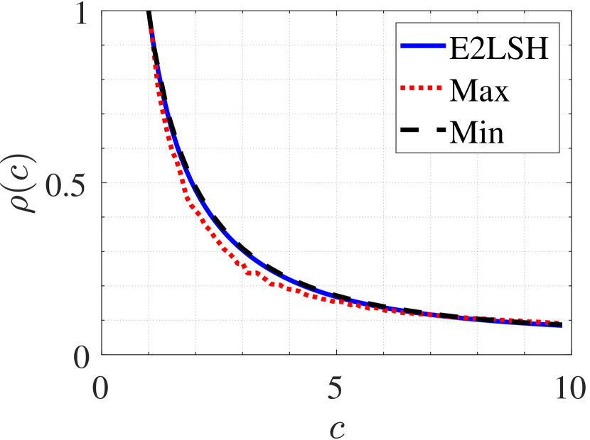
(c-3) Cifar: = 2.43 and = 10
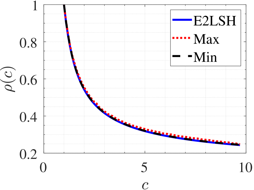
(d-1) Deep: = 0.5 and = 1.5
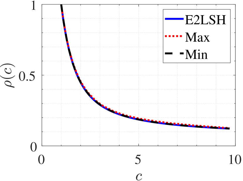
(d-2) Deep: = 1.36 and = 4
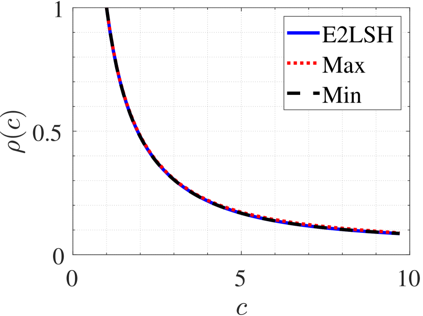
(d-3) Deep: = 3.4 and = 10
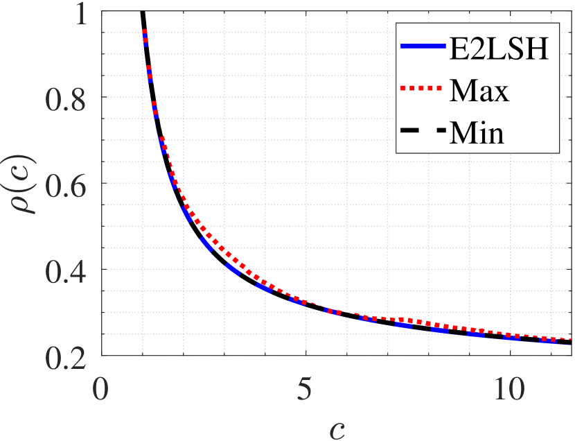
(e-1) Glove: = 0.81 and = 1.5
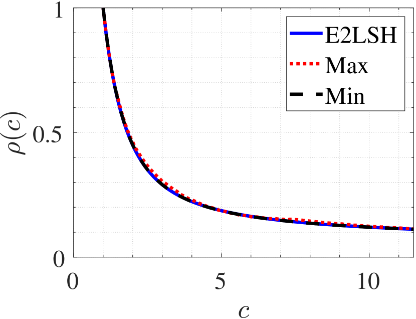
(e-2) Glove: = 2.2 and = 4
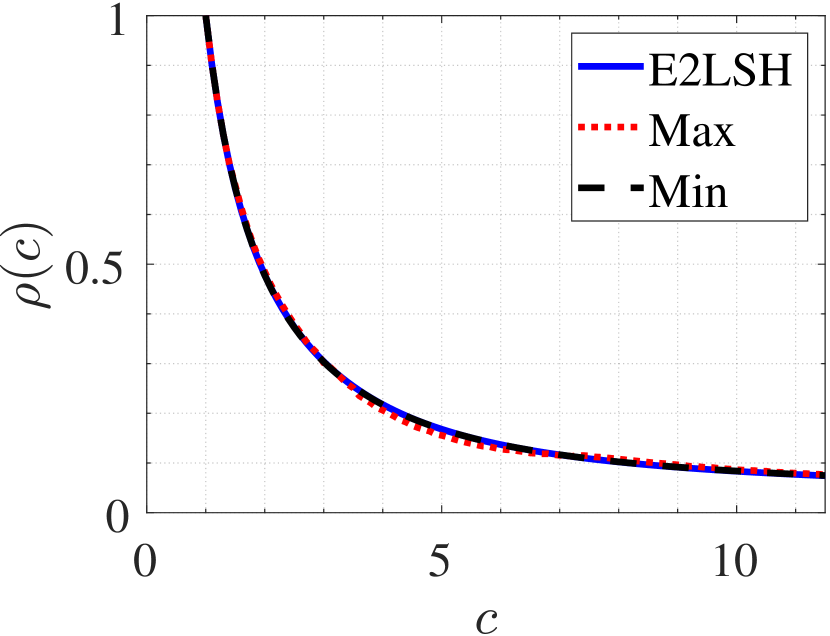
(e-3) Glove: = 5.45 and = 10
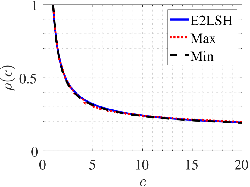
(a-1) ImageNet: = 0.635 and = 1.5
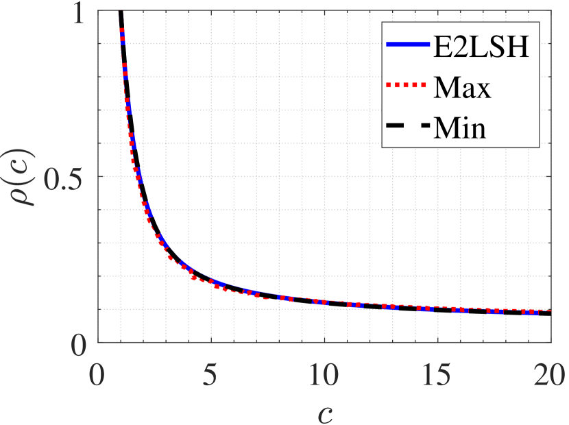
(a-2) ImageNet: = 1.8 and = 4
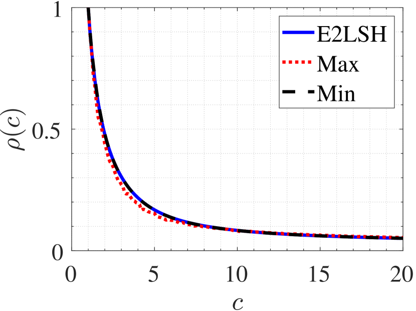
(a-3) ImageNet: = 4.45 and = 10
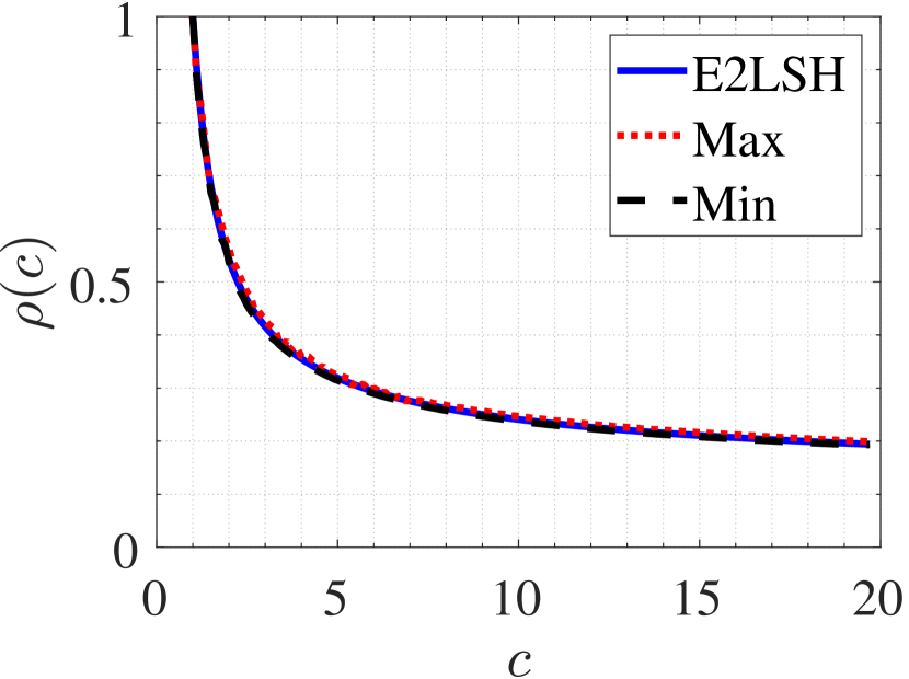
(b-1) Notre: = 0.69 and = 1.5
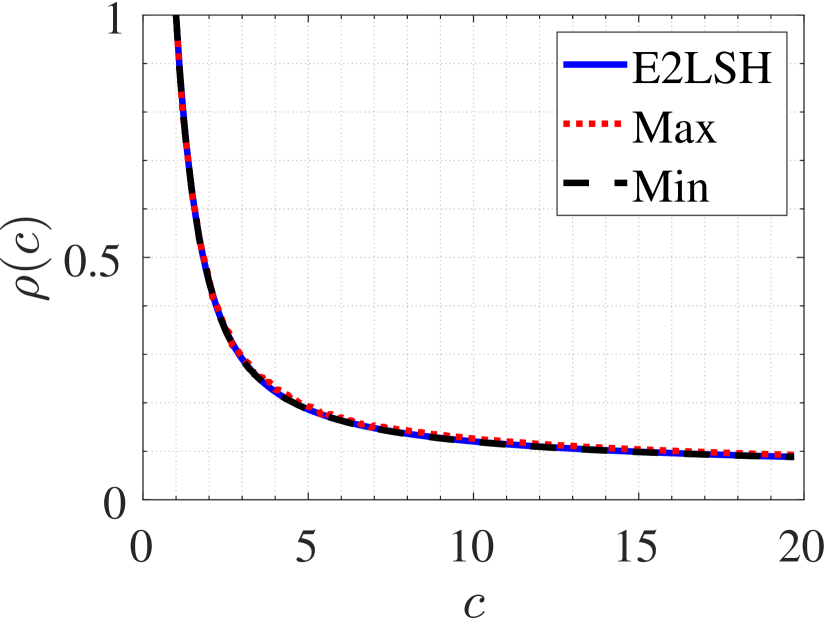
(b-2) Notre: = 1.9 and = 4

(b-3) Notre: = 4.75 and = 10
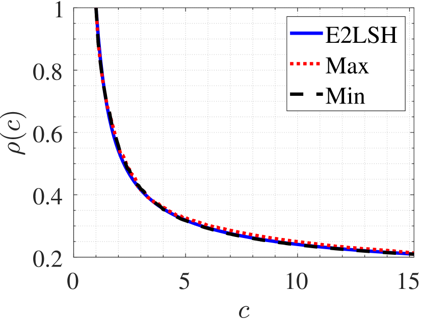
(c-1) Sift: = 0.68 and = 1.5
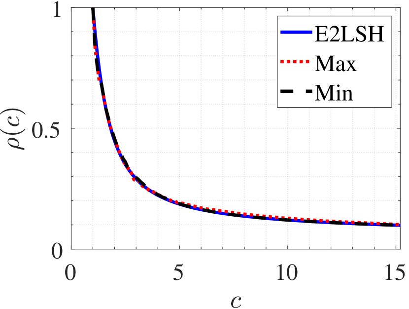
(c-2) Sift: = 1.9 and = 4
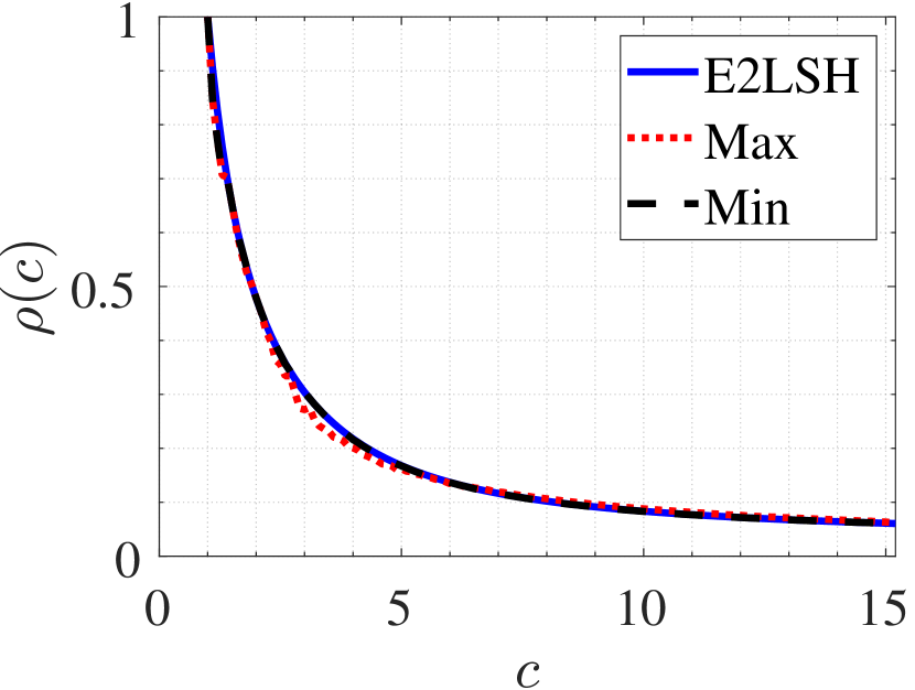
(c-3) Sift: = 4.75 and = 10
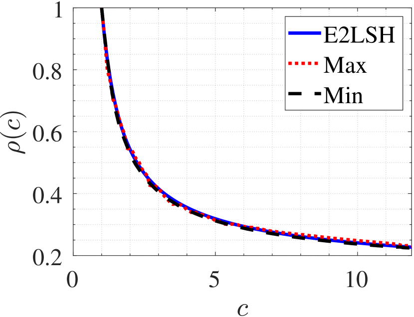
(d-1) Sun: = 0.343 and = 1.5
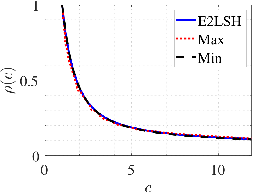
(d-2) Sun: = 0.98 and = 4
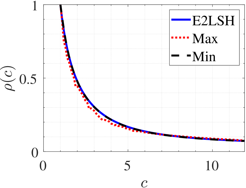
(d-3) Sun: = 2.4 and = 10
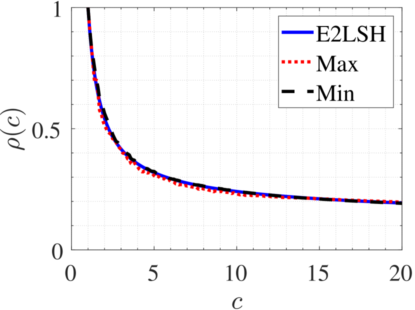
(e-1) Ukbench: = 0.7 and = 1.5
(e-2) Ukbench: = 2 and = 4
(e-3) Ukbench: = 4.95 and = 10
