Modeling Spatiotemporal Periodicity and Collaborative Signal for Local-Life Service Recommendation
Abstract.
Online local-life service platforms provide services like nearby daily essentials and food delivery for hundreds of millions of users. Different from other types of recommender systems, local-life service recommendation has the following characteristics: (1) spatiotemporal periodicity, which means a user’s preferences for items vary from different locations at different times. (2) spatiotemporal collaborative signal, which indicates similar users have similar preferences at specific locations and times. However, most existing methods either focus on merely the spatiotemporal contexts in sequences, or model the user-item interactions without spatiotemporal contexts in graphs. To address this issue, we design a new method named SPCS in this paper. Specifically, we propose a novel spatiotemporal graph transformer (SGT) layer, which explicitly encodes relative spatiotemporal contexts, and aggregates the information from multi-hop neighbors to unify spatiotemporal periodicity and collaborative signal. With extensive experiments on both public and industrial datasets, this paper validates the state-of-the-art performance of SPCS.
1. Introduction
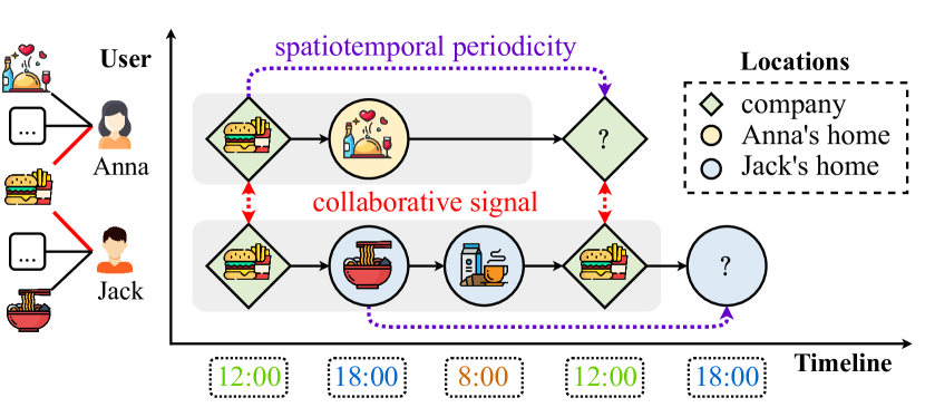
Online local-life service platforms, such as Meituan111http://i.meituan.com/ and Uber Eats222https://www.ubereats.com/, provide services like nearby daily essentials and food delivery for hundreds of millions of users. Different from other types of recommender systems (Zhou et al., 2018, 2019), local-life service recommendation has the following characteristics: (1) spatiotemporal periodicity, which means a user’s preferences for items vary from different locations at different times. According to the trajectory in Figure 1, Jack enjoys burgers at the company at noon, but he prefers noodles at home in the evening. (2) spatiotemporal collaborative signal, which means similar users exhibit similar preferences at specific locations and times. For instance, Anna and Jack share similar preferences while they are at the same company at noon. However, their preferences diverge in the evening due to their different home locations. Moreover, due to the strong coupling between these characteristics, it is crucial to directly incorporate spatiotemporal information rather than separately considering spatial or temporal aspects. Overall, both two characteristics (purple arrow and red arrow in Figure 1) have important implications for local-life service recommendation yet have rarely been studied in existing works. In this paper, we focus on simultaneously modeling the spatiotemporal periodicity and collaborative signal in local-life service platforms.
Generally speaking, there are two relevant lines of research for local-life service recommendation as shown in Table 1. One is the sequential-based recommender. The majority of studies (Liu et al., 2016; Sun et al., 2020; Luo et al., 2021; Lian et al., 2020; Cui et al., 2021) apply recurrent neural networks with spatiotemporal contexts between current and future steps to capture the transitional regularities in sequences. However, they ignore the spatiotemporal collaborative signal and fail to capture preferences from similar users. Another line of research is the graph-based recommender. Earlier works (Wang et al., 2019a; He et al., 2020) simply adopt GCN layers on the user-item interaction graph for collaborative filtering, ignoring the spatiotemporal contexts. Recent works (Ma et al., 2018; Fan et al., 2021; Rossi et al., 2020) aim to utilize spatial or temporal information in graphs. However, these methods either focus solely on the temporal information, or consider merely spatial information (location), which fail to model the spatiotemporal periodicity. In short, existing solutions leave a blank space in simultaneously modeling the spatiotemporal periodicity and collaborative signal for local-life service recommendation.
To address this issue, we propose a novel method, Modeling Spatiotemporal Periodicity and Collaborative Signal (SPCS) for local-life service recommendation. First, to capture the spatiotemporal contexts in graphs, we design the encoding layer, which explicitly encodes relative time interval as temporal encoding and relative spatial distance as spatial encoding. Second, to simultaneously model the spatiotemporal periodicity and collaborative signal, we design a novel spatiotemporal graph transformer (SGT) layer, which utilizes two encodings and aggregates the spatiotemporal information from multi-hop neighbors. The main contributions of this paper are as follows:
-
•
We propose a novel SPCS method to simultaneously model the spatiotemporal periodicity and collaborative signal for local-life service recommendation. Specifically, we capture the spatiotemporal contexts in the encoding layer, and then aggregate this information from multi-hop neighbors in the spatiotemporal graph transformer (STG) layer.
-
•
We conduct extensive experiments on both real-world public and industrial datasets. Experimental results demonstrate the effectiveness of our proposed SPCS.
| Type | Model | Collaborative | Temporal Info | Spatial Info |
| Sequential-based | ST-RNN | ✓ | ✓ | |
| STAN | ✓ | ✓ | ||
| TiSASRec | ✓ | |||
| SLRC | ✓ | |||
| Graph-based | LightGCN | ✓ | ||
| SAE-NAD | ✓ | ✓ | ||
| TGSRec | ✓ | ✓ | ||
| TGN | ✓ | ✓ | ||
| Our method | SPCS | ✓ | ✓ | ✓ |
2. Related Works
Sequential-based Recommenders. Most of the earlier works like GRU4Rec (Wu et al., 2019) and TiSASRec (Li et al., 2020) adopt sequential methods, such as RNN (Medsker and Jain, 2001) and self-attention (Vaswani et al., 2017), to capture the temporal evolution of user preferences. Besides, some other works (Liu et al., 2016; Cui et al., 2021; Luo et al., 2021) like ST-RNN (Liu et al., 2016) and STAN (Luo et al., 2021) aim to utilize spatiotemporal contexts between current and future steps to capture the transitional regularities. However, these methods ignore the spatiotemporal collaborative signal, which is essential to capture preferences from similar users at specific locations and times.
Graph-based Recommenders. Early works like NGCF (Wang et al., 2019a) and LightGCN (He et al., 2020) simply adopts GCN layers on the user-item interaction graph without using spatiotemporal contexts. Later works (Ma et al., 2018; Han et al., 2020; Yang et al., 2022) exploit the extensive collaborative signals for item-item relations with location information. Some other works (Wang et al., 2019b; Fan et al., 2021; Rossi et al., 2020; Tian et al., 2022; Chi et al., 2022; Bei et al., 2023) like TGSRec (Fan et al., 2021) and TGN (Rossi et al., 2020) attempt different utilization of time intervals with time-decaying functions to capture the temporal collaborative signal. However, these methods fail to fully utilize the spatiotemporal contexts and ignore the spatiotemporal periodicity. Therefore, we aim to simultaneously model the spatiotemporal periodicity and collaborative signal for local-life service recommendation.
3. Methodology
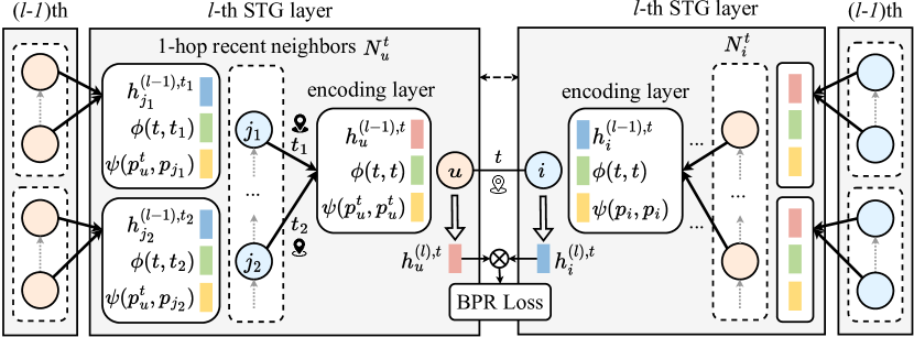
In this section, we first present related terms and formalize the problem of local-life service recommendation, then introduce the three main parts of our SPCS: (1) encoding layer, which explicitly encodes the spatiotemporal contexts as temporal encoding and spatial encoding. (2) spatiotemporal graph transformer layer, which combines two encodings and aggregates the information from multi-hop neighbors. (3) the prediction and optimization. Figure 2 illustrates the overall structure of SPCS.
3.1. Problem Formulation
Definition 1.
Spatiotemporal User-Item Graph is defined as , where and is the set of users and items, is a set of spatiotemporal edges. Each edge is denoted as a quintuple, , where , , , , and is a set of locations with latitude and longitude. Each means that a user will interact with item at time , traveling from location to location . We denote the neighbor set for user in the time interval as .
Definition 2.
Local-Life Service Recommendation. Given a spatiotemporal user-item graph and a new query tuple , local-life service recommendation aims to recommend item list that user would be interested at time and location .
3.2. Encoding Layer
3.2.1. User/Item Embedding
To maintain each user’s (item’s) history in a compressed format, we adopt a widely-used memory mechanism (Rossi et al., 2020). First, the memory state for a user (item ) at time is denoted as () , initialized as an all-zero vector and updated by the memory mechanism. Then, we define as the hidden embedding that serves as the input to the -th layer for user at time (the same applies to the hidden embedding for item ). Note that, in the first layer, . When , it is generated from the previous layer.
3.2.2. Temporal Encoding (TE)
Inspired by recent works (Xu et al., 2020; Fan et al., 2021), the periodicity can be reflected by relative time intervals between the user’s different interactions. We design the temporal encoding function as based on Bochner’s Theorem (Loomis, 2013) to encode the time intervals into embedding explicitly. Specifically, given two time points and , we implement as:
| (1) |
where is the cosine function. and are learnable weights and bias of linear transformation for the time interval.
3.2.3. Spatial Encoding (SE)
To quantify the change of locations between different users and items, we design the spatial encoding function as to derive the geographical weight. Specifically, given two locations and , we implement as:
| (2) |
where denotes the Haversine formula (Robusto, 1957), which is widely used to calculate the distance from latitude and longitude. is used to control the decay rate of the weight. And is a mapping function, such as an identity or exponential function. Note that other effective spatial encoding can also be explored and used in future work.
3.3. Spatiotemporal Graph Transformer Layer
In this section, we will introduce the spatiotemporal graph transformer (SGT) layer in two parts: (1) construction of query, key, and value; (2) spatiotemporal self-attention. In the following, we take the calculation for user at time as an example.
3.3.1. Construction of Query, Key and Value
To unify the spatiotemporal information and collaborative signal, we construct the input information of each SGT layer as the combination of hidden node embeddings, temporal encoding, and spatial encoding. Specifically, given the query user , we construct the query vector for user itself at -th layer as:
| (3) |
where the layer number . And is the vector concatenate operation and is the product operation in this paper. Other operations including summation are possible. In addition to query user itself, we also propagate spatiotemporal collaborative information from its neighbors. We sample most recent neighbors of user from . Similar to the construction of the query vector, the key/value matrix for user ’s most recent neighbors can be formulated as:
| (4) |
3.3.2. Spatiotemporal Self-Attention
Then, we adopt a self-attention mechanism to propagate the information as follows:
| (5) |
where is the softmax function. are learnable transformation matrices at -th layer.
By stacking layers, we can obtain the final embedding for user as . Analogously, for item , we need to alternate the user information to item information, and change the neighbor information in Eq. (3), (4) and (5) according to user-item pairs. Thus, for item can also be calculated. The time complexity of the proposed SPCS is .
3.4. Prediction and Optimization
For each , we can calculate the affinity score between user and item at time . To optimize parameters, we utilize the widely-used pairwise BPR loss (Rendle et al., 2009) for top-K recommendation, which can be formulated as:
| (6) |
where denotes the pairwise training data, and is the sigmoid function. denotes the regularization for addressing over-fitting.
4. Experiment
4.1. Experimental Settings
| Dataset | #User | #Item | #Instance | Timespan |
| Gowalla-Food | 15,058 | 26,594 | 553,121 | 2009.1.21-2010.3.11 |
| Meituan | 17,862 | 26,236 | 649,101 | 2022.2.14-2022.3.28 |
| Model | Gowalla-Food | Meituan | ||||||
| Hit@10 | Hit@20 | NDCG@10 | NDCG@20 | Hit@10 | Hit@20 | NDCG@10 | NDCG@20 | |
| ST-RNN | 0.02640.0002 | 0.03970.0001 | 0.01890.0001 | 0.02220.0001 | 0.01850.0002 | 0.03570.0003 | 0.00980.0001 | 0.01310.0001 |
| STAN | 0.19710.0021 | 0.24590.0025 | 0.14430.0021 | 0.15630.0023 | 0.08460.0008 | 0.13510.0011 | 0.04210.0008 | 0.04850.0011 |
| TiSASRec | 0.03960.0017 | 0.06300.0023 | 0.02140.0011 | 0.02720.0012 | 0.07930.0007 | 0.12760.0001 | 0.04090.0001 | 0.05300.0001 |
| SLRC | 0.18370.0014 | 0.22620.0008 | 0.13900.0012 | 0.14410.0015 | 0.10530.0010 | 0.16500.0016 | 0.05160.0011 | 0.05800.0011 |
| LightGCN | 0.03370.0001 | 0.05620.0003 | 0.01090.0001 | 0.01420.0001 | 0.03800.0002 | 0.06460.0002 | 0.01790.0001 | 0.02050.0001 |
| SAE-NAD | 0.08730.0043 | 0.13140.0049 | 0.05410.0019 | 0.06780.0020 | 0.05550.0013 | 0.09380.0022 | 0.03790.0008 | 0.05120.0012 |
| TGSRec | 0.15950.0163 | 0.21410.0116 | 0.10710.0205 | 0.12080.0194 | 0.06190.0007 | 0.09980.0010 | 0.03150.0006 | 0.04090.0006 |
| TGN | 0.24400.0046 | 0.30410.0029 | 0.16920.0064 | 0.18430.0059 | 0.09020.0037 | 0.14480.0076 | 0.04680.0024 | 0.06040.0033 |
| SPCS | 0.35760.0007 | 0.39310.0014 | 0.29310.0010 | 0.30210.0008 | 0.18630.0013 | 0.26620.0026 | 0.10730.0007 | 0.12730.0008 |
Dataset. We conduct experiments on two real-world datasets: Gowalla-Food (Liu et al., 2014) and Meituan. Gowalla-Food is a location-based service network for recommendation research. The Meituan dataset is collected from one of the largest local-life service platforms in China. Each interaction contains a user-ID, item-ID, timestamp, and GPS locations. For each dataset, we use the 10-core settings in (He et al., 2020) and chronologically split for train, validation, test in 8:1:1. This means we use the most recent 10% interactions for testing, which can be regarded as a multi-step sequential recommendation task. The statistics of all datasets are summarized in Table 2.
Baselines. We compare our SPCS with baselines in two categories (Table 1), including: (1) sequential-based methods, where ST-RNN (Liu et al., 2016), STAN (Luo et al., 2021), TiSASRec (Li et al., 2020), and SLRC (Wang et al., 2019b) utilize spatial or temporal information to capture the dynamic preferences of users; (2) graph-based methods, where LightGCN (He et al., 2020), SAE-NAD (Ma et al., 2018), TGSRec (Fan et al., 2021), and TGN (Rossi et al., 2020) capture the collaborative signal and utilize the temporal information from multi-hop neighbors.
Implementation and Evaluation. We implement our SPCS with PyTorch (Paszke et al., 2019) and conduct experiments on Tesla V100 (32GB). We search the node dimension and time dimension from {64, 128, 256}. The learning rate is selected from {1e-3, 1e-4, 1e-5}, and the layer number is selected from {1, 2, 3}. For recent neighbor sampling number , we search from {10, 20, 30}. We fix function as identity and search from {1, 2, 5}. The best version is , lr = 1e-4, , , . For interaction in the test set, we perform a full ranking (He et al., 2020) with all item candidates to evaluate the top-K recommendation performance, including Hit@K and NDCG@K, where K in {10, 20}.
4.2. Overall Performance
Table 3 shows the performance comparison between our SPCS and baselines. The observations from the table are: (1) SPCS consistently outperforms all the baselines on two datasets. In particular, SPCS improves over the strongest baseline w.r.t Hit@10 by 0.1132 and 0.0961 on Gowalla-Food and Meituan datasets, respectively. The superiority of our SPCS lies in simultaneously modeling spatiotemporal periodicity with the encoding layer and spatiotemporal graph transformer layer. (2) In sequential-based methods, STAN performs best on Gowalla-Food dataset, while SLRC performs best on Meituan dataset. The reason is that SLRC adopts the Hawkes process to explicitly model the temporal periodicity on Meituan dataset. However, they ignore the spatiotemporal collaborative signal so that they perform worse than our SPCS. (3) TGN performs best in graph-based methods. This is because TGN captures collaborative signals with temporal information in dynamic graphs. However, it ignores the spatiotemporal periodicity, especially the spatial information, which makes it worse than our SPCS.
4.3. Model Analysis of SPCS
4.3.1. Ablation Study
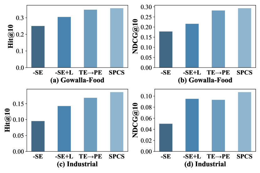
We further conduct an ablation study with several variants to validate the contributions of two encodings in SPCS: (1) -SE, in which spatial encoding is not used; (2) -SE+L, in which spatial encoding is not used but the recall is based on location within 5km; (3) TEPE, which replaces temporal encoding with position encoding. Table 3 reports the performance of these variants on two datasets. Here, we can make the following observations: (1) variant -SE suffers severe performance degradation on two datasets, which demonstrates the importance of spatial encoding in local-life service recommendation. (2) variant -SE+L improves the performance of variant -SE, but still performs worse than SPCS. This indicates the importance of spatial information, and propagating this information in graphs leads to better performance. (3) The performance degradation of variant TEPE also demonstrates the crucial role of temporal encoding.
4.3.2. Case Study
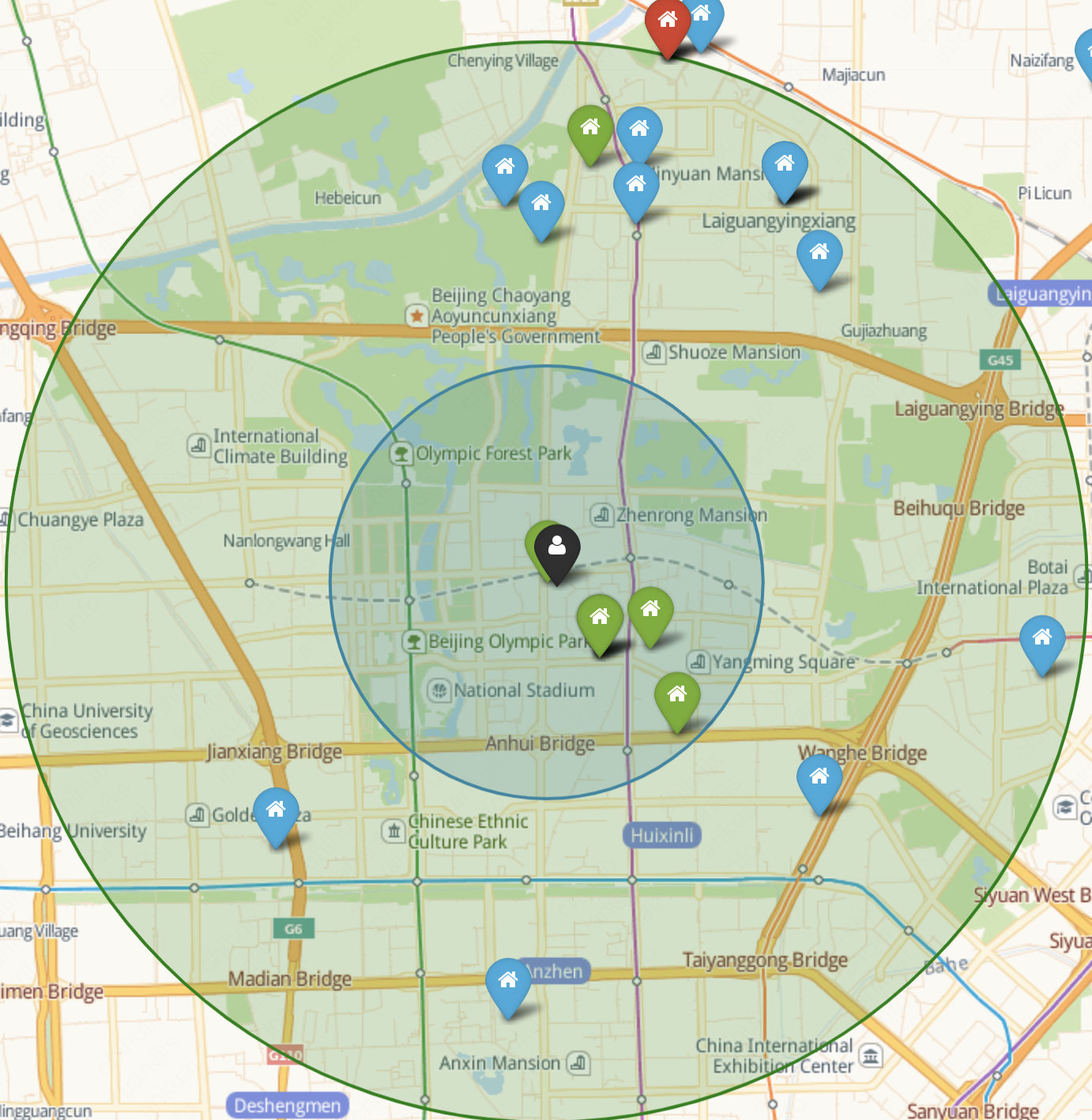
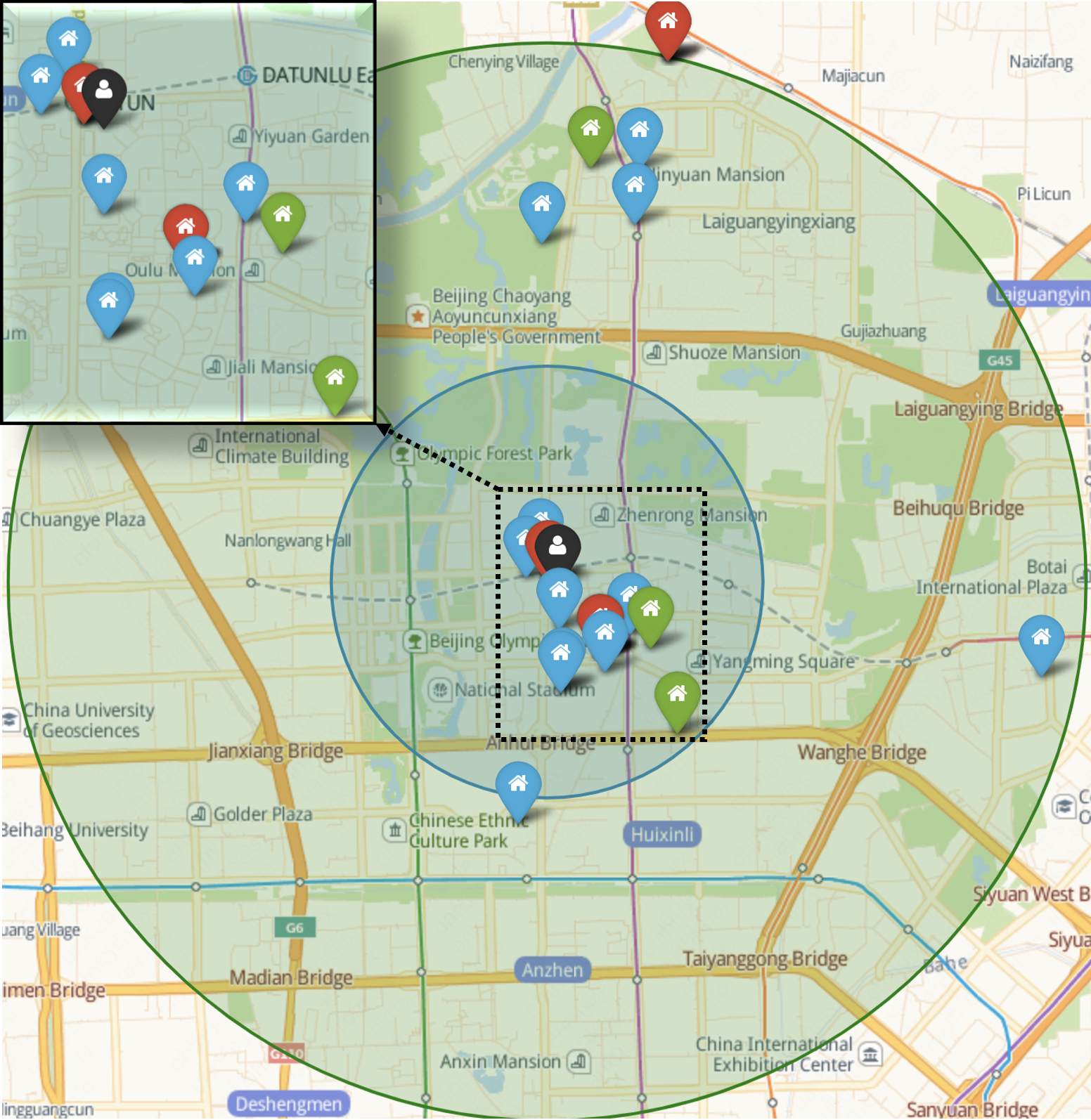
To further investigate the effectiveness of our SPCS, we conduct a case study comparing SPCS with TGN on Meituan dataset. As shown in Figure 4, the black mark denotes the user’s latest visited location, green marks denote the user’s target items at different times, blue marks denote the top-5 predicted items, and red marks denote the hit items. The inner blue circle and outer green circle denote a 2km and 5km radius, respectively. From the results, we find that the user’s target items are mostly located within 2km, and SPCS performs better than TGN in hitting these items. This further demonstrates the importance of simultaneously modeling the spatiotemporal periodicity and collaborative signal for local-life service recommendation.
5. Conclusion
In this paper, to simultaneously model the spatiotemporal periodicity and collaborative signal for local-life service recommendation, we propose a novel SPCS. To capture the spatiotemporal contexts in graphs, we design the encoding layer with temporal encoding and spatial encoding. To further capture the spatiotemporal periodicity and collaborative signal, we design a novel spatiotemporal graph transformer (SGT) layer, which aggregates the spatiotemporal information from multi-hop neighbors. Extensive experiments on both real-world public and industrial datasets demonstrate the effectiveness of our proposed SPCS.
References
- (1)
- Bei et al. (2023) Yuanchen Bei, Hao Xu, Sheng Zhou, Huixuan Chi, Mengdi Zhang, Zhao Li, and Jiajun Bu. 2023. CPDG: A Contrastive Pre-Training Method for Dynamic Graph Neural Networks. arXiv preprint arXiv:2307.02813 (2023).
- Chi et al. (2022) Huixuan Chi, Hao Xu, Hao Fu, Mengya Liu, Mengdi Zhang, Yuji Yang, Qinfen Hao, and Wei Wu. 2022. Long Short-Term Preference Modeling for Continuous-Time Sequential Recommendation. arXiv preprint arXiv:2208.00593 (2022).
- Cui et al. (2021) Qiang Cui, Chenrui Zhang, Yafeng Zhang, Jinpeng Wang, and Mingchen Cai. 2021. ST-PIL: Spatial-Temporal Periodic Interest Learning for Next Point-of-Interest Recommendation. In CIKM. 2960–2964.
- Fan et al. (2021) Ziwei Fan, Zhiwei Liu, Jiawei Zhang, Yun Xiong, Lei Zheng, and Philip S. Yu. 2021. Continuous-Time Sequential Recommendation with Temporal Graph Collaborative Transformer. In CIKM. 433–442.
- Han et al. (2020) Haoyu Han, Mengdi Zhang, Min Hou, Fuzheng Zhang, Zhongyuan Wang, Enhong Chen, Hongwei Wang, Jianhui Ma, and Qi Liu. 2020. STGCN: A Spatial-Temporal Aware Graph Learning Method for POI Recommendation. In ICDM. 1052–1057.
- He et al. (2020) Xiangnan He, Kuan Deng, Xiang Wang, Yan Li, Yongdong Zhang, and Meng Wang. 2020. Lightgcn: Simplifying and Powering Graph Convolution Network for Recommendation. In SIGIR. 639–648.
- Li et al. (2020) Jiacheng Li, Yujie Wang, and Julian McAuley. 2020. Time Interval Aware Self-Attention for Sequential Recommendation. In WSDM. 322–330.
- Lian et al. (2020) Defu Lian, Yongji Wu, Yong Ge, Xing Xie, and Enhong Chen. 2020. Geography-aware sequential location recommendation. In KDD. 2009–2019.
- Liu et al. (2016) Qiang Liu, Shu Wu, Liang Wang, and Tieniu Tan. 2016. Predicting the next location: A recurrent model with spatial and temporal contexts. In AAAI.
- Liu et al. (2014) Yong Liu, Wei Wei, Aixin Sun, and Chunyan Miao. 2014. Exploiting geographical neighborhood characteristics for location recommendation. In CIKM. 739–748.
- Loomis (2013) Lynn H Loomis. 2013. Introduction to abstract harmonic analysis.
- Luo et al. (2021) Yingtao Luo, Qiang Liu, and Zhaocheng Liu. 2021. Stan: Spatio-temporal attention network for next location recommendation. In WWW. 2177–2185.
- Ma et al. (2018) Chen Ma, Yingxue Zhang, Qinglong Wang, and Xue Liu. 2018. Point-of-interest recommendation: Exploiting self-attentive autoencoders with neighbor-aware influence. In CIKM. 697–706.
- Medsker and Jain (2001) Larry R Medsker and LC Jain. 2001. Recurrent neural networks. Design and Applications 5 (2001), 64–67.
- Paszke et al. (2019) Adam Paszke, Sam Gross, Francisco Massa, Adam Lerer, James Bradbury, Gregory Chanan, Trevor Killeen, Zeming Lin, Natalia Gimelshein, Luca Antiga, et al. 2019. Pytorch: An imperative style, high-performance deep learning library. NIPS 32 (2019).
- Rendle et al. (2009) Steffen Rendle, Christoph Freudenthaler, Zeno Gantner, and Lars Schmidt-Thieme. 2009. BPR: Bayesian Personalized Ranking from Implicit Feedback. In UAI. 452–461.
- Robusto (1957) C Carl Robusto. 1957. The cosine-haversine formula. The American Mathematical Monthly 64, 1 (1957), 38–40.
- Rossi et al. (2020) Emanuele Rossi, Ben Chamberlain, Fabrizio Frasca, Davide Eynard, Federico Monti, and Michael Bronstein. 2020. Temporal Graph Networks for Deep Learning on Dynamic Graphs. ICML’Workshop (2020).
- Sun et al. (2020) Ke Sun, Tieyun Qian, Tong Chen, Yile Liang, Quoc Viet Hung Nguyen, and Hongzhi Yin. 2020. Where to go next: Modeling long-and short-term user preferences for point-of-interest recommendation. In AAAI, Vol. 34. 214–221.
- Tian et al. (2022) Changxin Tian, Zihan Lin, Shuqing Bian, Jinpeng Wang, and Wayne Xin Zhao. 2022. Temporal Contrastive Pre-Training for Sequential Recommendation. In CIKM. 1925–1934.
- Vaswani et al. (2017) Ashish Vaswani, Noam Shazeer, Niki Parmar, Jakob Uszkoreit, Llion Jones, Aidan N Gomez, Łukasz Kaiser, and Illia Polosukhin. 2017. Attention is all you need. NIPS 30 (2017).
- Wang et al. (2019b) Chenyang Wang, Min Zhang, Weizhi Ma, Yiqun Liu, and Shaoping Ma. 2019b. Modeling item-specific temporal dynamics of repeat consumption for recommender systems. In WWW. 1977–1987.
- Wang et al. (2019a) Xiang Wang, Xiangnan He, Meng Wang, Fuli Feng, and Tat-Seng Chua. 2019a. Neural Graph Collaborative Filtering. SIGIR (2019), 165–174. arXiv:1905.08108
- Wu et al. (2019) Shu Wu, Yuyuan Tang, Yanqiao Zhu, Liang Wang, Xing Xie, and Tieniu Tan. 2019. Session-Based Recommendation with Graph Neural Networks. AAAI 33 (2019), 346–353. arXiv:1811.00855
- Xu et al. (2020) Da Xu, Chuanwei Ruan, Evren Korpeoglu, Sushant Kumar, and Kannan Achan. 2020. Inductive Representation Learning on Temporal Graphs. In ICLR.
- Yang et al. (2022) Song Yang, Jiamou Liu, and Kaiqi Zhao. 2022. GETNext: trajectory flow map enhanced transformer for next POI recommendation. In SIGIR. 1144–1153.
- Zhou et al. (2019) Guorui Zhou, Na Mou, Ying Fan, Qi Pi, Weijie Bian, Chang Zhou, Xiaoqiang Zhu, and Kun Gai. 2019. Deep Interest Evolution Network for Click-Through Rate Prediction. AAAI 33 (2019), 5941–5948.
- Zhou et al. (2018) Guorui Zhou, Xiaoqiang Zhu, Chenru Song, Ying Fan, Han Zhu, Xiao Ma, Yanghui Yan, Junqi Jin, Han Li, and Kun Gai. 2018. Deep interest network for click-through rate prediction. In KDD. 1059–1068.