Spatio-temporal correlations of noise in MOS spin qubits

Abstract

In quantum computing, characterising the full noise profile of qubits can aid the efforts towards increasing coherence times and fidelities by creating error mitigating techniques specific to the type of noise in the system, or by completely removing the sources of noise. Spin qubits in MOS quantum dots are exposed to noise originated from the complex glassy behaviour of two-level fluctuators, leading to non-trivial correlations between qubit properties both in space and time. With recent engineering progress, large amounts of data are being collected in typical spin qubit device experiments, and it is beneficiary to explore data analysis options inspired from fields of research that are experienced in managing large data sets, examples include astrophysics, finance and climate science. Here, we propose and demonstrate wavelet-based analysis techniques to decompose signals into both frequency and time components to gain a deeper insight into the sources of noise in our systems. We apply the analysis to a long feedback experiment performed on a state-of-the-art two-qubit system in a pair of SiMOS quantum dots. The observed correlations serve to identify common microscopic causes of noise, as well as to elucidate pathways for multi-qubit operation with a more scalable feedback system.

Introduction

Solid-state devices are suitable for qubit systems due to their high tunability, but they are exposed to noise originating from the material stack. The noise acting on solid-state qubit systems can be complex, including non-Markovian noise [1, 2, 3], and spatially and temporally correlated noise [4]. In order to increase the fidelities of qubits so that error correction protocols can be implemented, noise should be well understood [5, 6, 7] and qubits should retain quantum coherence long enough to perform useful calculations. There are efforts in mitigating and measuring noise in qubit systems [2, 8, 9, 10, 11, 12, 13, 3], including some focus on correlated noise [14, 15, 4] with work aimed towards understanding the microscopic origin of noise using correlations [4]. In this regard, using a qubit as a probe to investigate noise in solid state-devices can be effective.

In qubit devices, the dynamics and coherence of the system are perturbed by various sources of noise. The presence of correlations within the device parameters are a result of the perturbations being a function of position and time that evolve slowly compared to the separation between qubits or their typical operation time. Temporal correlations manifest as a dependence on previous events, while spatial on the location of the qubit within the device. The field of qubit error mitigation has made significant progress towards suppressing correlated noise contributions to qubit dynamics.

Spin qubits in silicon-based systems have achieved two-qubit gate fidelities above $99\%$ [16, 17, 18, 19, 20], but there remains unexplained noise that presents itself within the $1\%$ infidelity. Any improvement within this $1\%$ can have great repercussions in terms of number of qubits required in error correction codes [21] and further understanding of the noise could lead to tailored codes for types of noise specific to a device [22] or the refining of control methods [23] for quantum information purposes.

It is essential to have a tool to apply to large data sets to be able to analyse them for noise characteristics. Recently, the amount of data collected from spin qubit systems has vastly increased due to the development of real-time logic with controllers supported by field-programmable gate arrays (FPGAs). With vast amounts of data being produced, it is natural to move to more advanced statistical techniques. To do this, we take inspiration from scientific communities that already manage large data sets [24, 25, 26] which often use wavelet-based analysis. Other spin dynamics studies based on ensembles have also leveraged wavelet methods [27, 28]. Using wavelets, signals can be described by a basis consisting of different widths and displacements of a wave localised in time [29], resulting in frequency information about the signal, as well as non-periodic time information that is necessary to study non-Markovian noise. This is in contrast to Fourier-based analysis that is specifically useful for identifying particular periodicities in data.

The present study employs wavelet-based analysis on a qubit system using a silicon metal-oxide-semiconductor (SiMOS) device comprising two qubits. We analyse feedback data performed with the aid of an FPGA tracking eight different single- and two-qubit parameters in a long ($>3\times 10^{4}$ s) experiment. The data contains information on noise that couples to the qubits directly. Wavelet-based analysis is used to extract information on the noise coupled to the feedback parameters through the wavelet transformation, as well as extracting correlations through the Pearson correlation coefficient and wavelet variance transformation [25]. This paper marks an initial attempt to utilise wavelet-based analysis on vast quantities of data to comprehend noise in solid-state qubit systems.

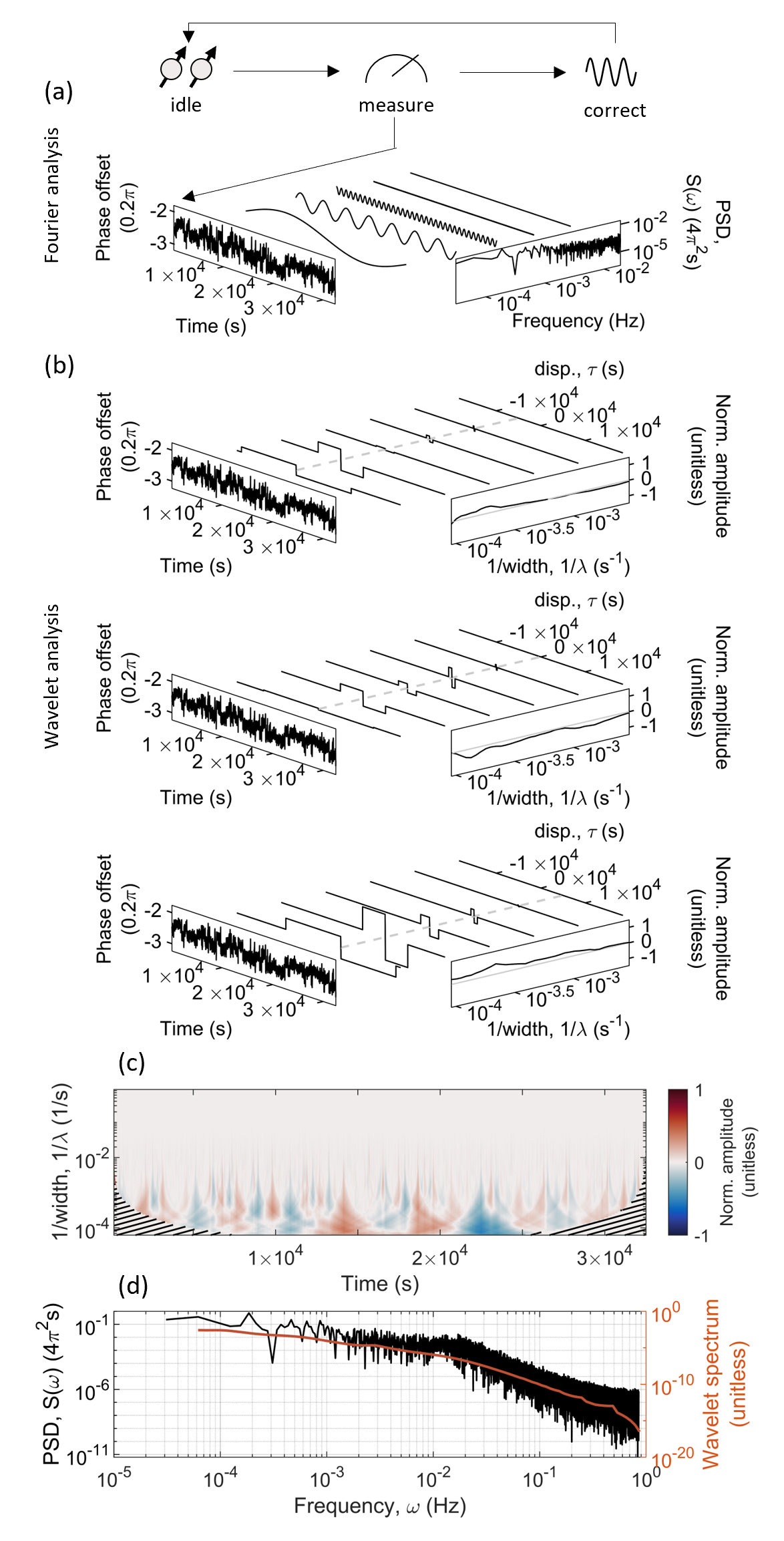
Figure 1: (a) Fourier analysis of qubit 1 phase feedback data. Left is a plot of the data, right is an inset of the power spectral density of the data, and the middle is the data decomposed into select frequencies. Above this is a simple representation of the experiment. (b) Wavelet analysis of qubit 1 phase feedback data. Left is a plot of the data, right is an inset of the wavelet transformation of the data normalised to the maximum value for displacements $\tau=-5\times 10^{4}$ s,$0$ s and $5\times 10^{4}$ s, and the middle is the data decomposed into select wavelet widths $\lambda$. (c) The full wavelet transformation of the data normalised to the maximum value. The lined section indicates the cone of influence. (d) The power spectral density in black and the wavelet spectrum in red.

Experiment

The qubits reside in a silicon substrate below a silicon dioxide interface, bound by the electric field created by an aluminium metal gate deposited on top of the oxide, resulting in a triangular potential formed at the interface between silicon and its oxide layer [30]. The potential arises from the differences in the electronic properties of silicon and silicon dioxide. The shape and height of the potential can be tuned by the voltage applied to the gate. This modulation of the potential allows for control of the electron density in the silicon channel; multiple gate electrodes enable further tuning of the potential landscape resulting in quantum dots that contain a controlled number of electrons. In our case, three electrons reside in one of the dots where the two lowest energy electrons form a closed shell and do not interfere with the dynamics of the other electron that is used as the qubit [20, 31, 32, 33]. The other dot contains a single electron. More details on the device architecture can be found in Ref. [34].

The device is tuned to a regime where two quantum dots are formed. We define qubit 1 (Q1) as the left dot and qubit 2 (Q2) as the right dot written as (1,3), detailing the number of electrons in (Q1, Q2). The single electron spin states are Zeeman split by an in-plane magnetic field $B_{0}$, defining the Larmor frequency $g\mu_{B}B_{0}$ of each two-level system that can be used as a qubit ($g$ is the electron g-factor and $\mu_{B}$ is the Bohr magneton). The Larmor frequency is measured through a Ramsey experiment, where the electron spin direction is perpendicular to the $B_{0}$ field so that the rate of precession can be determined through projected measurements. To perform single-qubit gates, an alternating magnetic field $B_{1}$, perpendicular to $B_{0}$, is generated via an on-chip antenna that has microwave pulses applied to it. Transforming into the rotating frame set by the frequency of the microwave source [35], the electron spin precesses about the, now stationary, $B_{1}$ field causing Rabi oscillations [36] when the frequency of the microwave is resonant with the qubit Larmor frequency. The power of the microwave is an important factor in defining the magnitude of the Rabi frequency. Two-qubit interactions are realised through the exchange interaction present when there is an overlap between the two electron wavefunctions [20, 37]. The exchange interaction is controlled through gate electrodes that are placed between the dots. The voltage applied to the intermediate gate tunes the magnitude of the exchange interaction. To readout the state of the qubits, a Pauli spin blockade readout method called parity readout is implemented, which uses a single electron transistor to probe the charge movement of the electrons. Parity readout results in the single electron transistor detecting a charge movement from (1,3) to (0,4) if the spin states of the two electrons are anti-parallel (i.e. in a singlet state or $T_{0}$ triplet state), otherwise there is no charge movement [32, 31].

The data analysed in this work tracked eight parameters in a feedback experiment consisting of a two-qubit system left to shift over time, away from its calibrated specifications. The system parameters are left to shift for over $3\times 10^{4}$ s, with multiple feedback steps consisting of a measurement followed by a correction so that each parameter does not drift too far. This method of feedback is used to allow for long experiments to be performed on qubit systems without the whole system having to be re-calibrated when a large drift occurs [20]. Here, a full feedback measurement can take up to 0.57 s (consisting of approximately 20 shots) setting the smallest time-scale of noise we can analyse. The variables tracked are: the microwave power of both qubits, corresponding to the Rabi frequencies; the Larmor frequencies; the individual qubit phases acquired by pulsing the exchange control gate due to Stark shift, which we call qubit phases for short; the voltage applied to the exchange control gate to obtain a target exchange interaction, which we call exchange level for short; and the (1,3)-(0,4) charge transition, corresponding to the readout point. Each variable is measured, recorded, then corrected compared to an initial calibration test where the offset in the feedback is set to zero. Some variables could have benefited from more accurate initial calibration, as evidenced by a significant drift in the first 200 seconds of the data (cut off in Figs 1 and 2). More details on how these were measured and the full data sets can be found in Ref. [34].

Wavelet transformation

The wavelet transformation provides more information compared to the Fourier-based analysis because it offers both frequency and time representations of signals. This is illustrated in Fig. 1(a), which displays the decomposition of data into frequency components through Fourier analysis, and Fig. 1(b), which shows the decomposition of the signal into inverse width values ($1/\lambda$) and displacements of the centre of the wavelet along the time axix ($\tau$) through wavelet analysis. Fourier analysis is effective in revealing how the power of a signal varies over frequency and detecting periodic signals in data sets, as shown by the inset of power spectral density on the right axes and the visual representation of the data in the Fourier basis.

Wavelets are mathematical functions that are centred in time and are a useful tool for the analysis of time series [29, 25, 38]. We define the mother wavelet to be a unitless vector $\vec{\Psi}(t)=\Psi_{n}=(\Psi_{0},\Psi_{1},...,\Psi_{N-1})^{T}$ where $(T)$ is the transpose, $t=n\Delta t$ is time with an interval of $\Delta t$ and $n\in\{0..N-1\}$. The two basic properties of a wavelet are

$$\sum_{n=0}^{N-1}\Psi_{n}=0\hskip 14.22636pt\text{and}\hskip 14.22636pt\sum_{n=0}^{N-1}|\Psi_{n}|^{2}=1.$$ (1)

In this work we focus on the particular choice of the Haar wavelet [39], depicted in the time domain in Fig. 1(b). The mother wavelet can be displaced and scaled with $\tau$ and $\lambda$ such that a wavelet reads $\psi_{n}(\tau,\lambda)=\vec{\psi}[(t-\tau)/\lambda]$. The Haar wavelet function is given as

$$\vec{\psi}\bigg{(}\frac{t-\tau}{\lambda}\bigg{)} =\psi_{n}(\tau,\lambda)$$ (2)

$$=\left\{\begin{array}[]{ll}\frac{1}{2\sqrt{\lambda}},\hskip 22.76228pt\tau-\lambda<t\leq\tau;\\ -\frac{1}{2\sqrt{\lambda}},\hskip 32.72049pt\tau<t\leq\tau+\lambda;\\ 0,\hskip 35.56593pt\text{otherwise}.\end{array}\right.$$ (6)

From this definition, all non-zero components of the Haar wavelet cover a time of $2\lambda$.

The wavelet transform can analyse a time series $\vec{x}=x_{n}=(x_{0},x_{1},...,x_{N-1})^{T}$ [40]. The continuous wavelet transform applied to a discrete time series is expressed as

$$W(\tau,\lambda)=\sum_{n=0}^{N-1}x_{n}\psi_{n}^{*}(\tau,\lambda),$$ (7)

where $(*)$ is the complex conjugate, although we deal with the Haar wavelet which is real so the complex conjugate is not needed. The parameter $1/2\lambda$ is proportional to frequency $\omega$. For our analysis, we have opted to plot the wavelet transformations with frequency units as the vertical axis (instead of unitless) for ease of interpretation. A wavelet transformation on $x_{n}$ that runs over values of $\tau_{n}=n\Delta t$ and values of $\lambda_{k}=k\Delta t$, $k=\{1..K\}$ where $K=(N-1)\ \mathbf{div}\ 2$ (with $\mathbf{div}$ denoting integer division), results in the matrix

$$\bm{W}_{x}=\begin{pmatrix}W(\tau_{0},\lambda_{1})&&\ldots&&W(\tau_{0},\lambda_{K})\\ W(\tau_{1},\lambda_{1})&&\ldots&&W(\tau_{1},\lambda_{K})\\ \vdots&&\ddots&&\vdots\\ W(\tau_{N-1},\lambda_{1})&&\ldots&&W(\tau_{N-1},\lambda_{K})\end{pmatrix}$$ (8)

with dimensions $N\times K$ and in the same units as the variable $\vec{x}$. This example of the wavelet transformation runs over all possible $\tau$ and $\lambda$ values rendering the transformation overcomplete. A theory of discrete wavelets can remove the redundancies [41], however in our analysis of noise we retain all information.

In Fig. 1, the Q1 phase feedback data is decomposed into the Fourier and wavelet bases, shown in the left axes. Figure 1(b) shows insets of $\bm{W}_{x}$ normalised to the maximum value, where each individual plot has a different value of $\tau$. The data decomposition into wavelet basis is visualised by scaling the amplitude of the wavelets to $1/2\lambda$ such that $\sum_{n^{\prime}=0}^{N-1}|\psi_{n}(\tau,\lambda)|^{2}=2\lambda$. This visual representation is then multiplied by $\bm{W}_{x}$. The added information the wavelet transformation holds is shown in Fig. 1(c), showing the entire $1/\lambda$ and $\tau$ representation of the time series. The steps in the data are represented in the wavelet transformation as a positive or negative amplitude; a positive amplitude when the wavelet is in phase with a signal in the data (a transition in the data from large to small) and a negative amplitude when the wavelet is the opposite shape to a signal in the data (a transition from small to large). Where there is zero amplitude, there is no difference in the data between the sampled times.

A property of the wavelet transformation is that it is able to give insight into the spectral information in the signal. This is similar to that given by the power spectral density in Fourier analysis. To do this, the variance $\sigma^{2}$ of $\bm{W}_{x}$ is calculated for each $\lambda$. The power of the spectral information is then the square of the variance, $\sigma^{4}$, which we call the wavelet spectrum [29]. The Fourier power spectral density and the wavelet spectrum are compared in Fig. 1(d). Here, the full power spectral density is displayed in black [Fig. 1(a) only shows a small part of the same power spectral density] and the wavelet spectrum normalised to the sum of all variances, i.e. $\sigma^{4}/\sum\sigma^{4}$, is shown in red. Here, the wavelet spectrum qualitatively agrees with the Fourier specturm, although the Fourier spectrum is able to capture finer details in frequency. This comparison demonstrates their agreement and highlights that the wavelet transformation possesses information that is also found in Fourier analysis.

The wavelet analysis allows for the freedom of choice of the wavelet basis, allowing the emphasis of specific characteristics of the system being analysed. In our case, we chose the Haar wavelet due to the prevalence of random telegraph noise in our data, which appear as discrete jumps [see for example the Q1 phase data at $t\approx 2.2\times 10^{4}$ s in Figs 1(a) and (b)], resembling the shape of the Haar wavelet. The wavelet transformation allows for the identification of events happening at a given time, called edge-detection, which has been shown to work well in quantum systems for the example of reading out charge jumps in a solid state device [38]. Wavelets allow for better analysis of the correlation between signals, as different correlations may exist at different widths. Additionally, wavelets can help to identify correlations that may not be apparent in the unprocessed signal, but represent a significant proportion of the error budget for qubits with infidelity below $1\%$.

A limitation associated with the size of the data set is that the range of $1/\lambda$ values that a given wavelet can decompose the signal into is constrained by the need to allow the wavelet to decay to zero within the time of the signal. This means that experiments need to be long compared to the scale of features that one aims to study. There are also boundary effects that need to be considered, called the cone of influence, that informs us about what parts of the wavelet transformation can be trusted [29]. The cone of influence is shown in Figs 1(c) as the lined space increasing as $1/\lambda$ decreases. This is, again, to ensure the wavelet at the edges of the transformation have decayed to zero.

I Variance transformation

The wavelet variance is a useful tool in recognising significant time scales within a data set, useful for spectral analysis. An important tool is the variance transformation, in which time correlated data sets are used to enhance features in one another by identifying prominent features with a certain width $\lambda$ through its variance. We can refer to the variables as the predictor, $\vec{x}$, and response, $\vec{y}$. The variance transformation is introduced in Ref. [25] as a means to identify a meaningful predictor variable and formulate a predictive model between $\vec{x}$ and $\vec{y}$. The former identification step is what we are interested in applying to quantum systems. The terms predictor and response are used because the predictor variable is modified to improve the accuracy of forecasting the behaviour of the response variable.

The variance transform compares the response $\vec{y}$ to the wavelet transformation $\bm{W}_{x}$ of the predictor variable $\vec{x}$. This is done by calculating the covariance between $\vec{y}$ and $\bm{W}_{x}$. The result is a vector of covariances $\vec{C}=C_{\lambda}=(C_{1},C_{2},...,C_{K})^{T}$ that compares $\vec{y}$ to the wavelet transformation at a given $\lambda$, i.e.

$$\vec{C}^{T}=\frac{(\vec{y}-\vec{y}_{\bar{y}})^{T}\bm{W}_{x}}{N-1},$$ (9)

where $\vec{y}_{\bar{y}}=(\bar{y},\bar{y},...,\bar{y})^{T}$ is a vector of length $N$ with each entry defined as the mean $\bar{y}=\sum_{n=0}^{N-1}y_{n}/N$. The variance-transformed data is then

$$\vec{x}^{\prime}=\bm{W}_{x}\sigma_{x}\vec{C},$$ (10)

where $\sigma_{x}$ is the standard deviation of $\vec{x}$. The variance transform redistributes the variances for each $\lambda$ component in $\vec{x}$ according to $\vec{C}$. The result is a new time series $\vec{x}^{\prime}$ that exhibits similar spectral properties as $\vec{y}$.

The correlation between two sets of data depends on the amplitude of the signals when dealing with the covariance. We can use the variance transformation to focus on the high amplitude signals between the data sets. This method is particularly useful for identifying the main sources of noise in an experiment. Alternatively, we can use the Pearson correlation coefficient, also known as the $r$-value, to see how correlated the signals are regardless of their amplitude. Both methods are explored in this work.

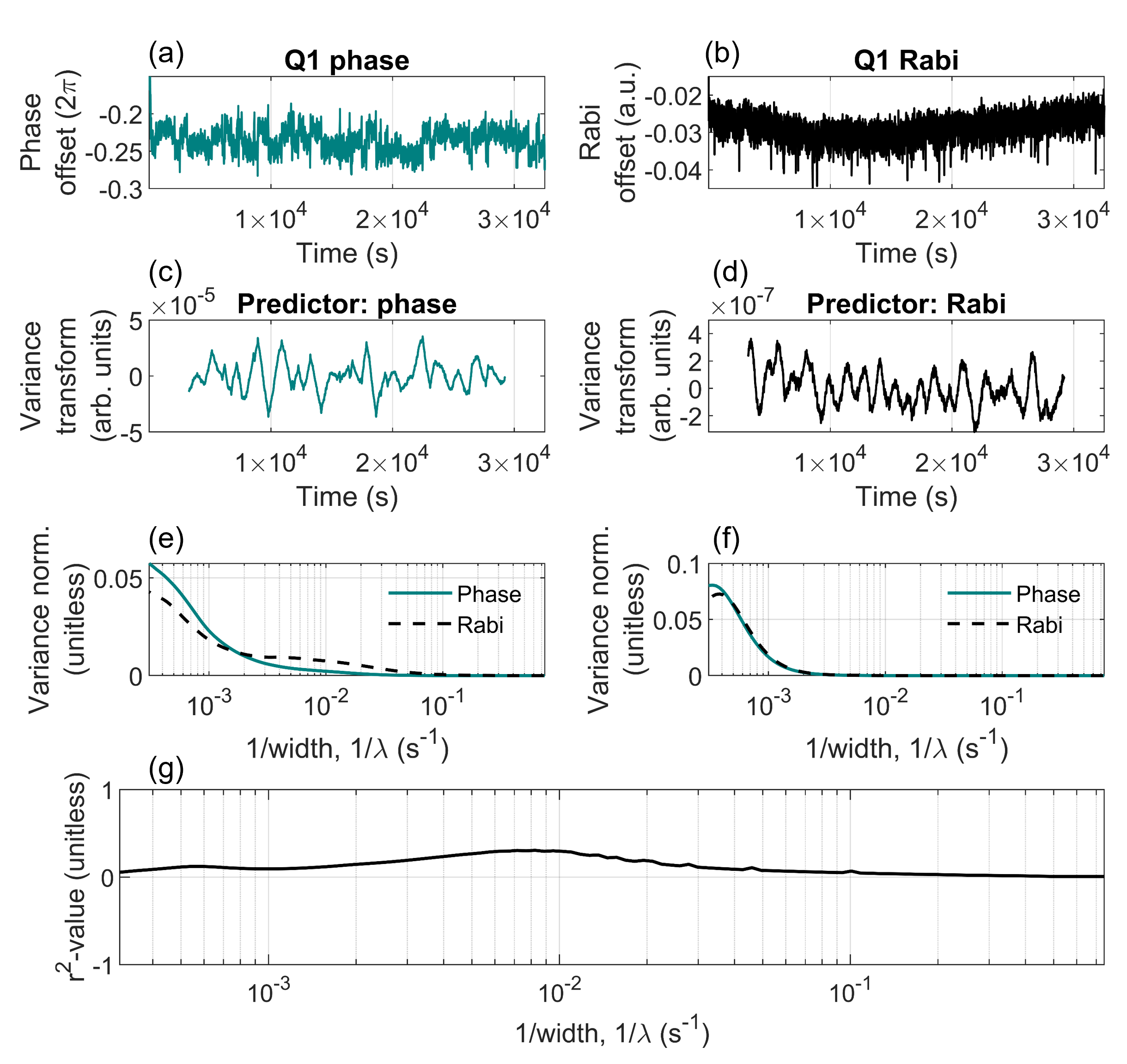
Figure 2: (a) Qubit 1 phase feedback data, (b) qubit 1 Rabi feedback data. Both (a) and (b) start at an offset of zero, but this data is not shown; the full data sets can be found in Ref. [34]. The variance transformed data sets with (c) the qubit 1 phase data as the predictor variable and (d) the qubit 1 Rabi feedback data as the predictor variable. The variance normalised to the sum of the variances for (e) the raw data wavelet transformation for the phase (blue) and Rabi (black dashed), and (f) the variance transformed data for the phase predictor (blue) and Rabi predictor (black dashed). (g) The Pearson correlation coefficient squared ($r^{2}$-value) calculated for each $1/\lambda$ of the wavelet transformed variables.

For the variance transformation method to be viable, all data sets being compared must have the same time step. To achieve this, the data is formatted to have the same time step as the data with the largest step (in our case this is the Q1 Larmor frequency feedback) which involves removing intermediate data points. On top of this, as $1/\lambda$ decreases, the cone of influence increases and therefore there is a limit to the minimum $1/\lambda$ in $\bm{W}_{x}$ that can be used in the variance transformation. A cut-off $1/\lambda$ is chosen as the minimum value such that $80\%$ of the data remains trustworthy. For the Haar wavelet with the current data sets that is $1/\lambda=3.09316\times 10^{-4}$ s^-1.

For an example of the variance transformation, we study the Q1 phase [Fig.2(a)] and the Q1 Rabi [Fig.2(b)]. The variance transformation, Eq. 10, of the two data sets is taken for both cases of the predictor variable, shown in Figs 2(c) and (d) in the Haar basis. The variance transformation reshapes the predictor variable to exhibit similar features as the response variable. The variance spectra of both data sets for each $1/\lambda$ is plotted in Fig. 2(c) and the variance spectra of the variance transformed data sets are in (d). The variance spectra for the raw data shows that most of the noise in the two variables is low $1/\lambda$ noise (low frequency). The Rabi variance (black dashed line) also shows a contribution at $1/\lambda$ of approximately $10^{-2}$ s^-1 corresponding to high amplitude, fast oscillations. After the variance transformation, the variance spectra in Fig. 2(d) is telling us that the signal that dominates both data sets is the low $1/\lambda$ noise. The peak variance is telling us about the largest amplitude signal that is in both the data sets, useful in informing us about the noise in the system that is affecting the parameters the most.

The $r$-value is calculated to look at correlations between the variables for each $1/\lambda$ value of the wavelet transformation, where high (anti)correlation has an $r$-value of (-)1, and 0 means no correlation. The significance $p$-value of the $r$-value is chosen to be below 0.05 - anything above 0.05 is set to have an $r$-value of 0. Figure 2(e) show the $r^{2}$-values plotted as a function of $1/\lambda$. The choice of $r^{2}$-values is because this can be interpreted as the percentage of events occurring in variable 1 explaining events in variable 2 [42].

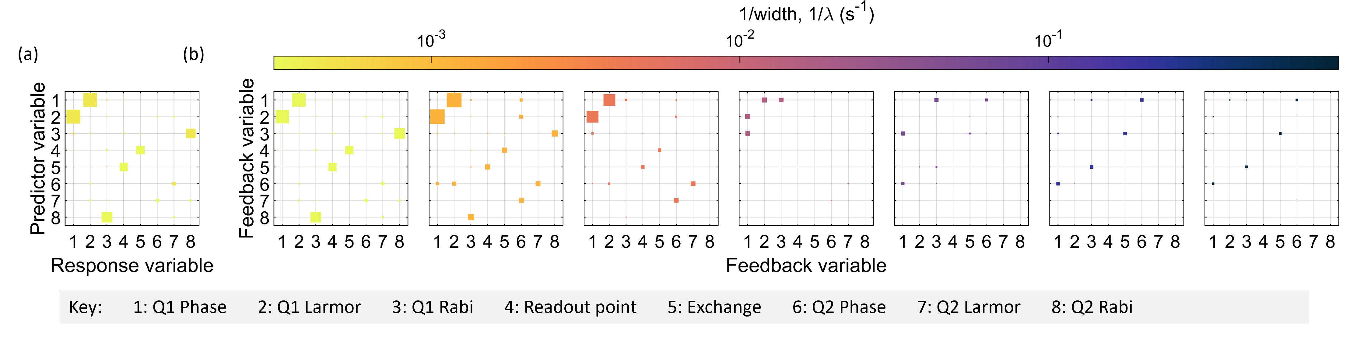
Figure 3: (a) The peak variance for the variance transformed data sets for each permutation of data set pairs. The size of the square corresponds to the square of the Pearson correlation coefficient, $r^{2}$-value, and the colour corresponds to $1/\lambda$. (b) The $r^{2}$-value for a range of $1/\lambda$ values. The key at the bottom indicates what the axes of the plots are showing.

Correlation analysis

The following section presents a visualisation of the relationships among the eight variables that were measured in the feedback experiment study (Ref. [34]). This visual representation serves as a tool for gaining a deeper understanding of the physics in the device and the experiment. To compare all the data, three steps are followed: first, we perform a wavelet transformation on each data set, second, we take the variance transformation for each permutation of data set pairs (permutations are used because the variance transformation is not symmetric), and third, we calculate the $r^{2}$-value for each wavelet transformation width for each data set.

Figure 3(a) shows a plot of the widths at which the maximum variance occurs in the variance transformation of the data sets using the Haar wavelet. The size of the squares represent the $r^{2}$-value and the colour indicates the value of $1/\lambda$. Most of the squares in the figure exhibit a peak variance for low values of $1/\lambda$, indicating that the primary high amplitude correlated noise source in the device is low frequency, which is typical for solid-state materials due to $1/f$ noise, where $f$ is frequency. It is important to note that high variance does not necessarily equate to high correlation (as indicated by the size of the square). This type of analysis is useful for identifying the largest sources of noise throughout the system.

Figure 3(b) displays the $r^{2}$-values for a range of $1/\lambda$ values for all pairs of data. The variables are arranged in a way such that the intra-qubit and temporal correlations are located in the top left and bottom right corners, while the inter-qubit temporal and spatial correlations are found in the top right and bottom left corners. This plot provides a more comprehensive view of the noise in the system. Because the wavelet analysis breaks down the data into different $1/\lambda$ contributions, it allows us to determine at what $1/\lambda$ the different noise sources influence the device, resulting in a deeper understanding of the physics of the noise. It is this improved understanding of noise that will aid the design of control pulses in quantum systems and the adaptation of error correction codes for quantum computing.

This method of correlation analysis is useful especially in the context of scalability for qubit systems. In our two qubit case study, there are already a lot of parameters that give information on the noise in the system. The variance transformation targets the high amplitude correlations in the system, practical for targeting noise that is impacting the system the most. For deeper analysis, Fig. 3(b) serves as a quick visualisation on what correlations are occurring, and specifically what type of correlations (spacial or temporal). This method of analysis is easily scaled to larger numbers of parameters, therefore useful for larger numbers of qubits. These kinds of analysis techniques should be fully developed before masses of qubits are created.

II Discussion

Throughout the text, the use of wavelets as a method to characterise noise has been mentioned. In this section, we will provide examples of the different types of noise in the system and explain how the wavelet transformation helped understand the noise.

A major source of noise in SiMOS qubits is low frequency, $1/f$ noise thought to be caused by an ensemble of two-level fluctuators [43, 44]. An intuitive way to look at $1/f$ noise is through spectral analysis which can be achieved using wavelets [45], shown in Fig. 1(d) from $\omega=0.3\times 10^{-4}$ to $10^{-2}$ Hz, where $\omega=1/2\lambda$. What is also shown in the wavelet spectrum is a bump at $\omega=10^{-}2$ Hz with a $1/\omega^{2}$ fall off, reminiscent of a fluctuator from the ensemble that is influencing the qubit environment at a larger magnitude [46]. The fluctuating signal can couple to an electron spin qubit either magnetically or electrically through the spin orbit interaction. For magnetic coupling, the fluctuator is likely to be a nuclear spin. The device used in the feedback experiment [34] is made on isotopically enriched silicon with 800ppm ²⁹Si nuclei resulting in a high probability of finding at least one nucleus that is hyperfine coupled to the electron qubits [47]. In time, a hyperfine coupled ²⁹Si nucleus flips, shifting the qubit Larmor frequency. For electrical coupling, the fluctuator is likely to be a trapped charge, tunnelling in and out of a defect in the device [44]. These two microscopic sources of noise can be distinguished because (i) the hyperfine interacting fluctuator is a contact interaction, meaning the fluctuating ²⁹Si only affects the electron that is in contact with it, and (ii) an electrically coupled fluctuator will also couple to parameters that are affected by the electrical environment and not the magnetic, i.e. the exchange and readout point.

The effects of a hyperfine coupled electron can be seen in Fig. 3(b) by studying the correlation magnitudes. Considering the Q1 phase and Q1 Larmor frequency, there is clearly a high magnitude correlation at $1/\lambda<10^{-2}$ s^-1. There are fluctuation signatures in the raw data sets [see for example Fig. 2(a)] at timescales that vary in size with frequencies that correspond to the high magnitude correlations at $1/\lambda<10^{-2}$ s^-1.

A correlation between the Q1 Larmor and Q1 phase is expected because a shift in the Larmor frequency results in a phase change with respect to the rotating frame because the phase is directly dependent on how fast the precession of the electron spin is about the $z$ axis. An important point to note is that there are no other variables that are highly correlated to the Q1 phase or Q1 Larmor, indicating no other variable has similar features at this time-scale. This, together with the discrete jumps in the data [Fig. 2(a)] and bump in the spectra [Fig. 1(d)] gives evidence for a nucleus hyperfine coupled to Q1. There are correlations between the exchange and the readout point that start to appear at $1/\lambda\lessapprox 5\times 10^{-3}$ s^-1. A correlation between these variables indicated an electrically coupled noise source - perhaps a fluctuator.

It is interesting that there are not a lot of inter-qubit correlations detected in the feedback data. The Q1 and Q2 Rabi data does show some correlation for $1/\lambda\lessapprox 5\times 10^{-3}$ s^-1. A very long time-scale drift is seen in the Q1 Rabi in Fig. 2(b), whose time-scale is a big as the entire experiment, so would show up as very highly correlated at $1/\lambda<1\times 10^{-3}$ s^-1. The correlation detected in Fig. 3(b) between the Rabi frequencies is probably due to this long drift, and experimentally can be attributed to the source of the $B_{0}$ magnetic field drifting.

III Outlook

Correlations are useful to understand the physical origin of noise in a system, as exemplified in the work in Ref. [4], we believe that using wavelet-based analysis such as that proposed in this work can aid in the modelling of noise in solid-state devices. If noise is well understood in qubit devices, then the development of control pulses for quantum systems will be optimised and error correction codes can be tailored for a particular hardware.

The challenge of scaling up the number of qubits in quantum computers poses several difficulties, including the need for a scalable method to measure noise in qubit systems and a scalable method to control noise through feedback protocols. The method presented for Fig. 3(b) shows how we can use wavelet techniques to analyse noise in a device in a scalable way - highlighting the contributions of noise at various $1/\lambda$ values. On top of this, the design of feedback protocols can be optimised by analysing correlations within the device. This can be achieved by eliminating redundant measurements when two variables are strongly correlated. The analysis shown in Fig. 3 can be used to identify these correlations and refine the feedback protocols, making them more efficient and suitable for large scale quantum computing.

Wavelet-based analysis has been employed in various fields such as climate science, finance, and traffic flow forecasting. These applications are particularly useful when external factors affect the forecast, as wavelet techniques are capable of isolating different time-scales. For instance, wavelet-based analysis has been used in climate sciences for weather prediction [25, 48], in finance for trading forecasting [49], and in traffic flow forecasting [50]. In future work, we aim to extend the use of wavelet analysis to qubit systems by characterising the time-scales of two-level fluctuators or other noise sources including the fact that there is the possibility of identifying different sources of $1/f$ noise from different ensembles of two-level fluctuators [51]. By forecasting the behaviour of qubit parameters in different time scales, we can gain insight into what may occur in the next time steps of an experiment, thereby improving qubit operation.

One of the benefits of wavelet analysis over Fourier analysis is the flexibility to select a basis that is customised to the system. Here, we used the Haar wavelet as the basis for analysis, but we also investigated the impact of using the bump basis. In the context of this work, there was no significant difference between the two wavelet bases.

Overall, this work applied wavelet-based methods to analyse correlations between eight parameters in a SiMOS two-qubit system. Due to the nature of the experiment, both spatially correlated and temporally correlated noise is extracted from the system. Gaining knowledge about these types of noise allows for better tailored error correction codes to be designed, and for scalability-specific error mitigation strategies to be developed. Wavelet analysis is particularly useful to aid the understanding of two-level fluctuator physics in solid-state devices due to the ability to detect discrete jumps in signals, together with the correlation analysis across multiple variables in a system. Specific to CMOS-based qubit hardware, wavelet-based analysis methods offer promising opportunities for system scalability, leading pathways to better understand the microscopic origins of noise within the devices. We see the use of wavelet analysis to be a useful in aiding the development of scalable qubit systems.

IV Acknowledgements

We acknowledge support from the Australian Research Council (FL190100167 and CE170100012), the US Army Research Office (W911NF-23-10092), and the NSW Node of the Australian National Fabrication Facility. The views and conclusions contained in this document are those of the authors and should not be interpreted as representing the official policies, either expressed or implied, of the Army Research Office or the US Government. The US Government is authorised to reproduce and distribute reprints for Government purposes notwithstanding any copyright notation herein. A.E.S, S.S., and J.Y.H. acknowledge support from the Sydney Quantum Academy.

References

- Burkard [2009] G. Burkard, Physical Review B 79, 125317 (2009).
- Chan et al. [2018] K. W. Chan, W. Huang, C. H. Yang, J. C. C. Hwang, B. Hensen, T. Tanttu, F. E. Hudson, K. M. Itoh, A. Laucht, A. Morello, and A. S. Dzurak, Physical Review Applied 10, 44017 (2018).
- Morris et al. [2019] J. Morris, F. A. Pollock, and K. Modi, arXiv preprint arXiv:1902.07980 (2019).
- Yoneda et al. [2022] J. Yoneda, J. S. Rojas-Arias, P. Stano, K. Takeda, A. Noiri, T. Nakajima, D. Loss, and S. Tarucha, arXiv preprint arXiv:2208.14150 (2022).
- Egan et al. [2021] L. Egan, D. M. Debroy, C. Noel, A. Risinger, D. Zhu, D. Biswas, M. Newman, M. Li, K. R. Brown, M. Cetina, and C. Monroe, Nature 598, 281 (2021).
- Abobeih et al. [2022] M. H. Abobeih, Y. Wang, J. Randall, S. J. H. Loenen, C. E. Bradley, M. Markham, D. J. Twitchen, B. M. Terhal, and T. H. Taminiau, Nature 606, 884 (2022).
- van Riggelen et al. [2022] F. van Riggelen, W. I. L. Lawrie, M. Russ, N. W. Hendrickx, A. Sammak, M. Rispler, B. M. Terhal, G. Scappucci, and M. Veldhorst, npj Quantum Information 8, 124 (2022).
- Muhonen et al. [2014] J. T. Muhonen, J. P. Dehollain, A. Laucht, F. E. Hudson, R. Kalra, T. Sekiguchi, K. M. Itoh, D. N. Jamieson, J. C. McCallum, A. S. Dzurak, and others, Nature nanotechnology 9, 986 (2014).
- Soare et al. [2014] A. Soare, H. Ball, D. Hayes, J. Sastrawan, M. C. Jarratt, J. J. McLoughlin, X. Zhen, T. J. Green, and M. J. Biercuk, Nature Physics 10, 825 (2014).
- Yoneda et al. [2018] J. Yoneda, K. Takeda, T. Otsuka, T. Nakajima, M. R. Delbecq, G. Allison, T. Honda, T. Kodera, S. Oda, Y. Hoshi, N. Usami, and others, Nature Nanotechnology 13, 102 (2018).
- Romach et al. [2015] Y. Romach, C. Müller, T. Unden, L. J. Rogers, T. Isoda, K. M. Itoh, M. Markham, A. Stacey, J. Meijer, S. Pezzagna, and others, Physical Review Letters 114, 17601 (2015).
- Bylander et al. [2011] J. Bylander, S. Gustavsson, F. Yan, F. Yoshihara, K. Harrabi, G. Fitch, D. G. Cory, Y. Nakamura, J.-S. Tsai, and W. D. Oliver, Nature Physics 7, 565 (2011).
- Almog et al. [2016] I. Almog, G. Loewenthal, J. Coslovsky, Y. Sagi, and N. Davidson, Physical Review A 94, 42317 (2016).
- Szańkowski et al. [2016] P. Szańkowski, M. Trippenbach, and . Cywiński, Physical Review A 94, 12109 (2016).
- von Lüpke et al. [2020] U. von Lüpke, F. Beaudoin, L. M. Norris, Y. Sung, R. Winik, J. Y. Qiu, M. Kjaergaard, D. Kim, J. Yoder, S. Gustavsson, L. Viola, and W. D. Oliver, PRX Quantum 1, 10305 (2020).
- Mills et al. [2022] A. R. Mills, C. R. Guinn, M. J. Gullans, A. J. Sigillito, M. M. Feldman, E. Nielsen, and J. R. Petta, Science Advances 8, 5130 (2022).
- Noiri et al. [2022] A. Noiri, K. Takeda, T. Nakajima, T. Kobayashi, A. Sammak, G. Scappucci, and S. Tarucha, Nature Communications 2022 13:1 13, 1 (2022).
- Ma̧dzik et al. [2022] M. T. Ma̧dzik, S. Asaad, A. Youssry, B. Joecker, K. M. Rudinger, E. Nielsen, K. C. Young, T. J. Proctor, A. D. Baczewski, A. Laucht, V. Schmitt, F. E. Hudson, K. M. Itoh, A. M. Jakob, B. C. Johnson, D. N. Jamieson, A. S. Dzurak, C. Ferrie, R. Blume-Kohout, and A. Morello, Nature 2022 601:7893 601, 348 (2022).
- Xue et al. [2022] X. Xue, M. Russ, N. Samkharadze, B. Undseth, A. Sammak, G. Scappucci, and L. M. K. Vandersypen, Nature 2022 601:7893 601, 343 (2022).
- Tanttu et al. [2023] T. Tanttu, W. H. Lim, J. Y. Huang, N. D. Stuyck, W. Gilbert, R. Y. Su, M. Feng, J. D. Cifuentes, A. E. Seedhouse, S. K. Seritan, C. I. Ostrove, K. M. Rudinger, R. C. C. Leon, W. Huang, C. C. Escott, K. M. Itoh, N. V. Abrosimov, H.-J. Pohl, M. L. W. Thewalt, F. E. Hudson, R. Blume-Kohout, S. D. Bartlett, A. Morello, A. Laucht, C. H. Yang, A. Saraiva, and A. S. Dzurak, arXiv preprint arXiv:2303.04090 (2023).
- Gidney and Ekerå [2021] C. Gidney and M. Ekerå, Quantum 5, 433 (2021).
- Ataides et al. [2021] J. P. B. Ataides, D. K. Tuckett, S. D. Bartlett, S. T. Flammia, and B. J. Brown, Nature Communications 12, 1 (2021).
- Yang et al. [2019] C. H. Yang, K. W. Chan, R. Harper, W. Huang, T. Evans, J. C. C. Hwang, B. Hensen, A. Laucht, T. Tanttu, F. E. Hudson, S. T. Flammia, K. M. Itoh, A. Morello, S. D. Bartlett, and A. S. Dzurak, Nature Electronics 2019 2:4 2, 151 (2019).
- Bijaoui [1999] A. Bijaoui, Wavelets in Physics (Cambridge University Press, 1999) pp. 77–116.
- Jiang et al. [2020] Z. Jiang, A. Sharma, and F. Johnson, Water Resources Research 56, e2019WR026962 (2020).
- In and Kim [2012] F. In and S. Kim, An Introduction to Wavelet Theory in Finance: A Wavelet Multiscale Approach (World Scientific Publishing Co., 2012) pp. 1–204.
- Phillies and Stott [1995] G. D. J. Phillies and J. Stott, Computers in Physics 9 (1995).
- Güldeste and Bulutay [2022] E. T. Güldeste and C. Bulutay, Physical Review B 105, 75202 (2022).
- Percival and Walden [2000] D. B. Percival and A. T. Walden, Cambridge University Press (2000).
- Ando et al. [1982] T. Ando, A. B. Fowler, and F. Stern, Reviews of Modern Physics 54, 437 (1982).
- Seedhouse et al. [2021] A. E. Seedhouse, T. Tanttu, R. C. C. Leon, R. Zhao, K. Y. Tan, B. Hensen, F. E. Hudson, K. M. Itoh, J. Yoneda, C. H. Yang, A. Morello, A. Laucht, S. N. Coppersmith, A. Saraiva, and A. S. Dzurak, PRX Quantum 2, 10303 (2021).
- Yang et al. [2020] C. H. Yang, R. C. C. Leon, J. C. C. Hwang, A. Saraiva, T. Tanttu, W. Huang, J. Camirand Lemyre, K. W. Chan, K. Y. Tan, F. E. Hudson, K. M. Itoh, A. Morello, M. Pioro-Ladrière, A. Laucht, and A. S. Dzurak, Nature 580, 350 (2020).
- Leon et al. [2021] R. C. C. Leon, C. H. Yang, J. C. C. Hwang, J. Camirand Lemyre, T. Tanttu, W. Huang, J. Y. Huang, F. E. Hudson, K. M. Itoh, A. Laucht, M. Pioro-Ladrière, A. Saraiva, and A. S. Dzurak, Nature Communications 12, 3228 (2021).
- Stuyck et al. [2023] N. D. Stuyck, A. E. Seedhouse, S. Serrano, T. Tanttu, W. Gilbert, J. Y. Huang, F. Hudson, K. M. Itoh, A. Laucht, W. H. Lim, C. H. Yang, A. Saraiva, and A. S. Dzurak, arXiv preprint arXiv:2309.12541 (2023).
- Vandersypen and Chuang [2004] L. M. K. Vandersypen and I. L. Chuang, Reviews of Modern Physics 76, 1037 (2004).
- Veldhorst et al. [2015] M. Veldhorst, C. H. Yang, J. C. C. Hwang, W. Huang, J. P. Dehollain, J. T. Muhonen, S. Simmons, A. Laucht, F. E. Hudson, K. M. Itoh, A. Morello, and A. S. Dzurak, Nature 526, 410 (2015).
- Meunier et al. [2011] T. Meunier, V. E. Calado, and L. M. K. Vandersypen, Physical Review B 83, 121403(R) (2011).
- Prance et al. [2015] J. R. Prance, B. J. Van Bael, C. B. Simmons, D. E. Savage, M. G. Lagally, M. Friesen, S. N. Coppersmith, and M. A. Eriksson, Nanotechnology 26, 215201 (2015).
- Haar [1911] A. Haar, Mathematische Annalen 71, 38 (1911).
- Torrence and Compo [1998] C. Torrence and G. P. Compo, Bulletin of the American Meteorological Society 79, 61 (1998).
- Daubechies [1988] I. Daubechies, Communications on Pure and Applied Mathematics 41, 909 (1988).
- Chen and Popovich [2002] P. Chen and P. Popovich, Sage University Papers Series on Quantitative Applications in the Social Sciences (2002).
- Machlup [1954] S. Machlup, Review of Scientific Instruments 25, 1681 (1954).
- Hooge [2003] F. N. Hooge, Physica B: Condensed Matter 336, 236 (2003).
- Wornell [1993] G. W. Wornell, Proceedings of the IEEE 81, 1428 (1993).
- Elsayed et al. [2022] A. Elsayed, M. Shehata, C. Godfrin, S. Kubicek, S. Massar, Y. Canvel, J. Jussot, G. Simion, M. Mongillo, D. Wan, R. Govoreanu, B., L. I. P., v. D. P. R., and K. de Greve, arXiv preprint arXiv:2212.06464 (2022).
- Hensen et al. [2020] B. Hensen, W. Wei Huang, C.-H. Yang, K. Wai Chan, J. Yoneda, T. Tanttu, F. E. Hudson, A. Laucht, K. M. Itoh, T. D. Ladd, A. Morello, and A. S. Dzurak, Nature nanotechnology 15, 13 (2020).
- Jiang et al. [2021] Z. Jiang, M. M. Rashid, F. Johnson, and A. Sharma, Environmental Modelling & Software 135, 104907 (2021).
- Al Wadi et al. [2011] S. Al Wadi, M. Tahir Ismail, M. H. Alkhahazaleh, S. Ariffin, and A. Karim, Applied Mathematical Sciences 5, 315 (2011).
- Li et al. [2023] H. Li, Z. Lv, J. Li, Z. Xu, W. Yue, H. Sun, and Z. Sheng, ACM Transactions on Knowledge Discovery from Data 17, 1 (2023).
- Principato and Ferrante [2007] F. Principato and G. Ferrante, Physica A: Statistical Mechanics and its Applications 380, 75 (2007).