Complexity analysis of regularization methods for implicitly constrained least squares

Abstract

Optimization problems constrained by partial differential equations (PDEs) naturally arise in scientific computing, as those constraints often model physical systems or the simulation thereof. In an implicitly constrained approach, the constraints are incorporated into the objective through a reduced formulation. To this end, a numerical procedure is typically applied to solve the constraint system, and efficient numerical routines with quantifiable cost have long been developed for that purpose. Meanwhile, the field of complexity in optimization, that estimates the cost of an optimization algorithm, has received significant attention in the literature, with most of the focus being on unconstrained or explicitly constrained problems.

In this paper, we analyze an algorithmic framework based on quadratic regularization for implicitly constrained nonlinear least squares. By leveraging adjoint formulations, we can quantify the worst-case cost of our method to reach an approximate stationary point of the optimization problem. Our definition of such points exploits the least-squares structure of the objective, and provides new complexity insights even in the unconstrained setting. Numerical experiments conducted on PDE-constrained optimization problems demonstrate the efficiency of the proposed framework.

1 Introduction

PDE-constrained optimization problems arise in various scientific and engineering fields where the objective is to find the optimal distribution of a given quantity while satisfying physical or mathematical laws described by PDEs, such as heat conduction or electromagnetic waves [1, 18, 13, 20]. Similar constrained formulations have also received recent interest from the machine learning community, as they opened new possibilities for building neural network architectures [17]. A popular approach to handle PDE constraints is the so-called reduced formulation, in which the constraints are incorporated into the objective and become implicit. By properly accounting for the presence of these constraints while computing derivatives, it becomes possible to generalize unconstrained optimization techniques to the implicitly constrained setting [18].

Algorithms designed for implicitly-constrained optimization in scientific computing are typically based on careful problem representation, that allow for the use of linear algebra routines in very high dimensions. The cost of the associated operations in terms of floating-point number calculations or memory use is often at the core of an efficient implementation. Nevertheless, the analysis of these methods usually does not account for the cost of the optimization routines themselves, and rather provides asymptotic convergence results. Although asymptotic convergence certifies that a given method is capable of reaching a solution of the problem, they do not quantify how fast an algorithm can be at satisfying a desired stopping criterion, or its performance under a constrained computational budget.

Providing such guarantees is the idea behind worst-case complexity analysis, a technique that has gained significant traction in the optimization community over the past decade, especially in the nonconvex setting [6]. A complexity bound characterizes the worst-case performance of a given optimization scheme according to a performance metric (e.g., number of iterations, derivative evaluations, etc) and a stopping criterion (e.g., approximate optimality, predefined budget, etc). Recent progress in the area has switched from designing optimization techniques with complexity guarantees in mind to studying popular algorithmic frameworks through the prism of complexity, with several results focusing on the least-squares setting [3, 4, 5, 10]. Despite this connection to practical considerations, complexity guarantees have yet to be fully explored, especially in the context of implicitly-constrained optimization.

In this paper, we study an algorithmic framework for least-squares problems with implicit constraints. Our approach leverages the particular structure of the objective in order to compute derivatives, and encompasses popular algorithms for nonlinear least squares such as the Levenberg-Marquardt method [15]. Under standard assumptions for this class of methods, we establish complexity guarantees for our framework. In a departure from standard literature, our analysis is based on a recently proposed stationarity criterion for least-squares problems [5]. To the best of our knowledge, these results are the first of their kind for implicitly constrained problems. In addition, our complexity results improve over bounds recently obtained in the unconstrained setting [4], thereby advancing our understanding of complexity guarantees for least-squares problems. Numerical experiments on PDE-constrained problems illustrate the practical relevance of the proposed stationarity criterion, and show that our framework handles both small and large residual problems, as well as nonlinearity in the implicit constraints.

The rest of this paper is organized as follows. In Section 2, we present our formulation of interest, and discuss how its least-squares structure is used to design our algorithmic framework. We establish complexity guarantees for several instances of our proposed method in Section 3. In Section 4, we investigate the performance of our algorithm on classical benchmark problems from PDE-constrained optimization. We finally summarize our work in Section 5.

2 Least-squares optimization with implicit constraints

In this paper, we discuss algorithms for least-squares problems of the form

$$\min_{u\in\mathbb{R}^{d}}J(y,u):=\frac{1}{2}\|R(y,u)\|^{2}\quad\operatorname*{subject\ to\ }\quad c(y,u)=0,$$ (1)

that involves both the variable $u$ (typically representing a control on a given system) as well as a vector of auxiliary variables $y$ (often reflecting the state of the system). We are interested in problems where it is possible to (numerically) solve the constraint equation $c(y,u)=0$ to obtain a unique solution $y$ given $u$. Problem (1) can then be reformulated as

$$\min_{u\in\mathbb{R}^{d}}J(y(u),u)=\frac{1}{2}\|R(y(u),u)\|^{2},$$ (2)

where the constraint arises implicitly in the formulation [12]. In PDE-constrained optimization, the constraint is a PDE, that can be solved given a value for the control vector $u$ to yield a state vector $y(u)$. In that setting, problem (2) is often called the reduced formulation [18, Chapter 1]. We are particularly interested in leveraging the least-squares nature of problem (1). To this end, we describe in Section 2.1 how derivatives can be computed by the adjoint approach for problem (2) while leveraging the problem structure. Our algorithm is then given in Section 2.2.

2.1 Computing adjoints for a least-squares problem

In this section, we derive an adjoint formula associated with the reduced formulation (2). Even though the analysis relies on standard arguments, to the best of our knowledge the formulas for the least-squares setting are rather unusual in the literature. We believe that they may be of independent interest, and therefore we provide the full derivation below.

To this end, we make the following assumption on our problem, which is a simplified version of a standard requirement in implicitly constrained problems [12].

Assumption 2.1

For any $u\in\mathbb{R}^{d}$, the following properties hold.

1. There exists a unique vector $y(u)$ such that $c(y,u)=0$.

2. The functions $J$ and $c$ are twice continuously differentiable.

3. The Jacobian of $c$ with respect to its first argument, denoted by $c_{y}(\cdot,\cdot)$, is invertible at any $(y,u)$ such that $c(y,u)=0$.

We now describe our approach for computing the Jacobian $G_{R}(y(u),u)$ given $u$, based on the adjoint equation. In what follows, we let $\hat{J}(u):=J(y(u),u)$ and $\hat{R}(u)=R(y(u),u)$ denote the reduced objective function and its associated residual function, respectively. It follows from the chain rule that

$$\nabla\hat{J}(u)=\nabla_{u}J(y(u),u)+c_{u}(y(u),u)^{\mathrm{T}}\lambda(u),$$ (3)

where $\lambda(u)$ is a solution of the so-called adjoint equation

$$c_{y}(y(u),u)^{\mathrm{T}}\lambda=-\nabla_{y}J(y(u),u).$$

This observation is at the heart of the adjoint method. In our case, we can leverage the least-squares of our problem to decompose (3) further. Indeed, the derivatives of $J$ with respect to its first and second arguments are given by

$$\left\{\begin{array}[]{lll}\nabla_{y}J(y(u),u)&=&G_{y}(y(u),u)^{\mathrm{T}}R(y(u),u)\\ \nabla_{u}J(y(u),u)&=&G_{u}(y(u),u)^{\mathrm{T}}R(y(u),u),\\ \end{array}\right.$$ (4)

where $G_{y}(y,u)$ and $G_{u}(y,u)$ are the Jacobian matrices with respect to $y$ and $u$. Plugging these expressions in (3), we obtain

$$\nabla\hat{J}(u) = \nabla_{u}J(y(u),u)+c_{u}(y(u),u)^{\mathrm{T}}\lambda(u)$$

$$= G_{u}(y(u),u)^{\mathrm{T}}R(y(u),u)+c_{u}(y(u),u)^{\mathrm{T}}\lambda(u)$$

$$= G_{u}(y(u),u)^{\mathrm{T}}R(y(u),u)-c_{u}(y(u),u)^{\mathrm{T}}\left[c_{y}(y(u),u)^{\mathrm{T}}\right]^{\dagger}\nabla_{y}J(y(u),u)$$

$$= G_{u}(y(u),u)^{\mathrm{T}}R(y(u),u)-c_{u}(y(u),u)^{\mathrm{T}}\left[c_{y}(y(u),u)^{\mathrm{T}}\right]^{\dagger}G_{y}(y(u),u)^{\mathrm{T}}R(y(u),u)$$

$$= \left[G_{u}(y(u),u)-G_{y}(y(u),u)c_{y}(y(u),u)^{\dagger}c_{u}(y(u),u)\right]^{\mathrm{T}}R(y(u),u)$$

$$= \left[G_{u}-G_{y}c_{y}(y(u),u)^{\dagger}c_{u}(y(u),u)\right]^{\mathrm{T}}R(y(u),u),$$

where $A^{\dagger}$ denotes the Moore-Penrose pseudo-inverse According to this expression, we can identify the Jacobian of $\hat{R}(u)$, which we denote by $\hat{G}(u)$, as

$$\hat{G}(u):=G_{u}-G_{y}c_{y}(y(u),u)^{\dagger}c_{u}(y(u),u).$$ (5)

Algorithm 1 summarizes the analysis below, and describes the adjoint method to compute derivative information when the objective has a least-squares structure.

Algorithm 1 Adjoint equations for implicitly constrained least squares

0:  Point of interest $u\in\mathbb{R}^{d}$ and vector $y(u)$ such that $c(y(u),u)=0$.

1:  Solve the equation

$$c_{y}(y(u),u)\zeta(u)=-K_{u}$$ (6)

for $\zeta(u)$.

2:  Compute $\hat{G}(u)=G_{u}+G_{y}\zeta(u)$.

In our main algorithm as well as its implementation, we will rely on Algorithm 1 to compute derivative information.

2.2 Algorithmic framework

Our optimization procedure is described in Algorithm 2. This method builds on the Levenberg-Marquardt paradigm [15] and more generally on quadratic regularization techniques.

At every iteration, the method computes a tentative step by approximately minimizing a quadratic model of the function. This step is then accepted or rejected depending on whether it produces sufficient function reduction compared to that predicted by the model. The $k$th iteration of Algorithm 2 will be called successful if $u_{k+1}\neq u_{k}$, and unsuccessful otherwise. The model is defined using a quadratic regularization parameter, that is decreased on successful iterations and increased on unsuccessful ones.

Algorithm 2 Regularization method for constrained least squares

0:  Initial iterate $u_{0}\in\mathbb{R}^{n}$; initial parameter $\gamma_{0}>0$; minimum regularization parameter $0<\gamma_{\min}\leq\gamma_{0}$; step acceptance threshold $\eta\in(0,1)$.  

1:  Solve the constraint $c(y,u_{0})=0$ for $y$ to obtain $y(u_{0})$.

2:  Evalue $R_{0}=R(y(u_{0}),u_{0})$ and the Jacobian $G_{0}=G_{R}(y(u_{0}),u_{0})$.

3:  for $k=0,1,2,\dotsc$ do

4:     Compute a step $s_{k}$ as an approximate solution to the following problem

$$\min_{s\in\mathbb{R}^{n}}m_{k}(u_{k}+s):=\frac{1}{2}\|R_{k}\|^{2}+g_{k}^{\mathrm{T}}s+\frac{1}{2}s^{\mathrm{T}}(H_{k}+\gamma_{k}I)s,$$ (7)

where $g_{k}=G_{k}^{\mathrm{T}}R_{k}$ is the gradient of $\hat{J}$ at $u_{k}$ and $H_{k}\in\mathbb{R}^{n\times n}$ is a symmetric matrix.

5:     Solve the constraint $c(y,u_{k}+s_{k})=0$ for $y$ to obtain $y(u_{k}+s_{k})$.

6:     Compute the ratio of actual to predicted decrease in $f$ defined as

$$\rho_{k}\leftarrow\frac{\hat{J}(u_{k})-\hat{J}(u_{k}+s_{k})}{m_{k}(u_{k})-m_{k}(u_{k}+s_{k})}.$$

7:     if $\rho_{k}\geq\eta$ then

8:        Set $u_{k+1}\leftarrow u_{k}+s_{k}$ and $\gamma_{k+1}\leftarrow\max\{0.5\gamma_{k},\gamma_{\min}\}$.

9:        Solve the constraint $c(y,u_{k+1})=0$ for $y$ to obtain $y(u_{k+1})$.

10:        Evaluate $R_{k+1}=R(y(u_{k+1}),u_{k+1})$ and the Jacobian $G_{k+1}=G_{R}(y(u_{k+1}),u_{k+1})$.

11:     else

12:        Set $u_{k+1}\leftarrow u_{k}$ and $\gamma_{k+1}\leftarrow 2\gamma_{k}$.

13:     end if

14:  end for

Note that our method can be instantiated in several ways, depending on the way $H_{k}$ is computed at every iteration, and on how the subproblem (7) is solved. In this paper, we assume that $H_{k}$ is built using only first-order derivative information, and consider two specific cases. When $H_{k}$ is the zero matrix, then the method can be viewed as a gradient method. When $H_{k}=G_{k}^{\mathrm{T}}G_{k}$, the method is a regularized Gauss-Newton iteration, similar to the Levenberg-Marquardt method. Although we focus on the two aforementioned cases in this paper, we point out that other formulae such as quasi-Newton updates [15] could also be used without the need for second-order information. As for the subproblem solve, we provide guarantees for exact and inexact variants of our framework in the next section.

3 Complexity analysis

In this section, we investigate the theoretical properties of Algorithm 2 through the lens of complexity. More precisely, we are interested in bounding the effort needed to reach a vector $u_{k}$ such that

$$\|R(y(u_{k}),u_{k})\|\leq\epsilon_{R}\quad\mbox{or}\quad\frac{\|G_{R}(y(u_{k}),u_{k})^{\mathrm{T}}R(y(u_{k}),u_{k})\|}{\|R(y(u_{k}),u_{k})\|}\leq\epsilon_{g}.$$ (8)

Condition (8) implicitly distinguishes between two kinds of approximate stationary points. When possible, one would ideally compute a point for which the residuals are small, or a stationary point for the norm of the residual. This scaled gradient condition was previously used for establishing complexity guarantees for algorithms applied to nonlinear least-squares problems [4, 5, 11].

Section 3.1 provides an iteration complexity bound for all instances of the algorithm.

3.1 Iteration complexity

We begin by a series of assumptions regarding the reduced formulation (2).

Assumption 3.1

The function $\hat{J}:u\mapsto J(y(u),u)$ is continuously differentiable in $u$. Moreover, the gradient of $\hat{J}$ with respect to $u$ is $L$-Lipschitz continuous for $L>0$.

Note that the first part of Assumption 3.1 is implied by Assumption 2.1.

Assumption 3.2

There exists a positive constant $M_{H}>0$ such that $\|H_{k}\|\leq M_{H}$ for all $k$.

Assumption 3.2 is trivially satisfied when $H_{k}$ is the zero matrix, or whenever the iterates are contained in a compact set. In addition to boundedness, we make an additional requirement on that matrix.

Assumption 3.3

For any iteration $k$, the matrix $H_{k}$ is chosen as a positive semidefinite matrix.

Note that both the zero matrix and the Gauss-Newton matrix $G_{k}^{\mathrm{T}}G_{k}$ are positive semidefinite, and thus satisfy Assumption 3.3.

Lemma 3.1

Let Assumptions 3.1,3.2 and 3.3 hold. Suppose that the subproblem (7) is solved exactly at iteration $k$. Then,

$$s_{k}=-(H_{k}+\gamma_{k}I)^{-1}G_{k}^{\mathrm{T}}R_{k}$$ (9)

where $I$ is the identity matrix in $\mathbb{R}^{d\times d}$. Moreover,

$$m_{k}(u_{k})-m_{k}(u_{k}+s_{k})\geq\frac{1}{2}\frac{\|G_{k}^{\mathrm{T}}R_{k}\|^{2}}{M_{H}+\gamma_{k}}.$$ (10)

Proof. Under Assumption 3.3, the subproblem (7) is a strongly convex quadratic subproblem. It thus possesses a unique global minimum given by $-(H_{k}+\gamma_{k}I)^{-1}G_{k}^{\mathrm{T}}R_{k}$, which is precisely (9). Using this formula for $s_{k}$, we obtain

$$m_{k}(u_{k})-m_{k}(u_{k}+s_{k}) \geq -R_{k}^{\mathrm{T}}G_{k}s_{k}-\frac{1}{2}s_{k}^{\mathrm{T}}(H_{k}+\gamma_{k}I)s_{k}$$

$$= R_{k}^{\mathrm{T}}G_{k}(H_{k}+\gamma_{k}I)^{-1}G_{k}^{\mathrm{T}}R_{k}-\frac{1}{2}R_{k}^{\mathrm{T}}G_{k}(H_{k}+\gamma_{k}I)^{-1}G_{k}^{\mathrm{T}}R_{k}$$

$$= \frac{1}{2}R_{k}^{\mathrm{T}}G_{k}(H_{k}+\gamma_{k}I)^{-1}G_{k}^{\mathrm{T}}R_{k}$$

$$\geq \frac{1}{2}\frac{\|G_{k}^{\mathrm{T}}R_{k}\|^{2}}{\|H_{k}+\gamma_{k}I\|}.$$

By Assumption 3.2, we have

$$\|H_{k}+\gamma_{k}\|\leq\|H_{k}\|+\gamma_{k}\leq M_{H}+\gamma_{k}.$$

Hence, we have

$$m_{k}(u_{k})-m_{k}(u_{k}+s_{k})\geq\frac{1}{2}\frac{\|G_{k}^{\mathrm{T}}R_{k}\|^{2}}{M_{H}+\gamma_{k}},$$

as required. $\Box$

Our second ingredient for a complexity proof consists in bounding the value of the regularization parameter.

Lemma 3.2

Let Assumptions 3.1, 3.3 and 3.2 hold. Then,

1. If $k$ is the index of an unsuccessful iteration, then $\gamma_{k}<\tfrac{L}{2(1-\eta)}$.

2. For any iteration $k$,

   $$\gamma_{k}\leq\gamma_{\max}:=\max\left\{1,\gamma_{0},\frac{L}{1-\eta}\right\}.$$ (11)

Proof. Suppose that the $k$th iteration is unsuccessful, i.e. that $\rho_{k}<\eta$. Then, one has

$$\eta(m_{k}(u_{k}+s_{k})-m_{k}(u_{k}))<\hat{J}(u_{k}+s_{k})-\hat{J}(u_{k}).$$ (12)

Using Assumption 3.1, a Taylor expansion of $\hat{J}$ around $u_{k}$ yields

$$\hat{J}(u_{k}+s_{k})-\hat{J}(u_{k}) \leq \nabla\hat{J}(u_{k})^{\mathrm{T}}s_{k}+\frac{L}{2}\|s_{k}\|^{2}$$

$$= g_{k}^{\mathrm{T}}s_{k}+\frac{L}{2}\|s_{k}\|^{2}$$

$$= m_{k}(u_{k}+s_{k})-m_{k}(u_{k})-\frac{1}{2}s_{k}^{\mathrm{T}}(H_{k}+\gamma_{k}I)s_{k}+\frac{L}{2}\|s_{k}\|^{2}$$

$$\leq m_{k}(u_{k}+s_{k})-m_{k}(u_{k})+\frac{L}{2}\|s_{k}\|^{2},$$

where the last inequality holds because of Assumption 3.3. Combining this inequality with (12), we obtain that

$$\eta(m_{k}(u_{k}+s_{k})-m_{k}(u_{k})) < \hat{J}(u_{k}+s_{k})-\hat{J}(u_{k})$$

$$\Rightarrow\eta(m_{k}(u_{k}+s_{k})-m_{k}(u_{k})) < m_{k}(u_{k}+s_{k})-m_{k}(u_{k})+\frac{L}{2}\|s_{k}\|^{2}$$

$$\Rightarrow(1-\eta)(m_{k}(u_{k})-m_{k}(u_{k}+s_{k})) < \frac{L}{2}\|s_{k}\|^{2}.$$

From Lemma 3.1, we obtain both an expression for $s_{k}$ and a bound on the left-hand side. Noting that

$$\|s_{k}\|\leq\frac{\|G_{k}^{\mathrm{T}}R_{k}\|}{\|H_{k}+\gamma_{k}I\|}\leq\frac{\|G_{k}^{\mathrm{T}}R_{k}\|}{M_{H}+\gamma_{k}},$$

we obtain

$$(1-\eta)(m_{k}(u_{k})-m_{k}(u_{k}+s_{k})) < \frac{L}{2}\|s_{k}\|^{2}$$

$$\Leftarrow\frac{(1-\eta)}{2}\frac{\|G_{k}^{\mathrm{T}}R_{k}\|^{2}}{M_{H}+\gamma_{k}} < \frac{L}{2}\frac{\|G_{k}^{\mathrm{T}}R_{k}\|^{2}}{(M_{H}+\gamma_{k})^{2}}$$

$$\Leftrightarrow\frac{1-\eta}{2(M_{H}+\gamma_{k})} < \frac{L}{2(M_{H}+\gamma_{k})^{2}}$$

$$\Leftrightarrow\gamma_{k} < \frac{L}{(1-\eta)}-M_{H}<\frac{L}{(1-\eta)}.$$

Overall, we have shown that if the $k$th iteration is unsuccessful, then necessarily $\gamma_{k}<\tfrac{L}{(1-\eta)}$. By a contraposition argument, we then obtain that $\gamma_{k}\geq\tfrac{L}{(1-\eta)}$ implies that the iteration is successful and that $\gamma_{k+1}\leq\gamma_{k}$. Combining this observation with the initial value of $\gamma_{0}$ and the update mechanism for $\gamma_{k}$, we find that $\gamma_{k}$ can never exceed $\max\{\gamma_{0},\frac{L}{1-\eta}\}\leq\gamma_{\max}$, proving the desired result. $\Box$

We stress out that we choose $\gamma_{max}$ to be greater than or equal to $1$ in order to simplify our bounds later on, but that the analysis below extends to the choice $\gamma_{\max}=\max\{\gamma_{0},\tfrac{L}{1-\eta}\}$.

We now provide our first iteration complexity bound, that focuses on successful iterations.

Lemma 3.3

Let Assumptions 3.1, 3.2 and 3.3 hold. Let $\epsilon_{g}\in(0,1)$, and let ${\cal S}_{\epsilon_{g},\epsilon_{R}}$ denote the set of successful iterations for which $u_{k}$ does not satisfy (8). Then,

$$\left|S_{\epsilon_{g},\epsilon_{R}}\right|\quad\leq\quad\left\lceil\mathcal{C}_{{\cal S}}\log(2\hat{J}(u_{0})\epsilon_{R}^{-2})\epsilon_{R}^{-2}\right\rceil+1,$$ (13)

where $\mathcal{C}_{{\cal S}}=\tfrac{M_{H}+\gamma_{\max}}{\eta}$.

Proof. Let $k\in{\cal S}_{\epsilon_{g},\epsilon_{R}}$. By definition, the corresponding iterate $u_{k}$ satisfies

$$\|R_{k}\|\geq\epsilon_{R}\quad\mbox{and}\quad\frac{\|G_{k}^{\mathrm{T}}R_{k}\|}{\|R_{k}\|}\geq\epsilon_{g}.$$ (14)

Moreover, since $k$ corresponds to a successful iteration, we have $\rho_{k}\geq\eta$, i.e.

$$\hat{J}(u_{k})-\hat{J}(u_{k+1})\geq\eta\left(m_{k}(u_{k})-m_{k}(u_{k}+s_{k})\right)\geq\eta\frac{\|G_{k}^{\mathrm{T}}R_{k}\|^{2}}{2(M_{H}+\gamma_{k})}\geq\eta\frac{\|G_{k}^{\mathrm{T}}R_{k}\|^{2}}{2(M_{H}+\gamma_{\max})},$$

where we used the results of Lemmas 3.1 and 3.2 to bound the model decrease and $\gamma_{k}$, respectively. Combining the last inequality with (14) leads to

$$\hat{J}(u_{k})-\hat{J}(u_{k+1}) \geq \frac{\eta}{2(M_{H}+\gamma_{\max})}\|G_{k}^{\mathrm{T}}R_{k}\|^{2}$$

$$= \frac{\eta}{2(M_{H}+\gamma_{\max})}\frac{\|G_{k}^{\mathrm{T}}R_{k}\|^{2}}{\|R_{k}\|^{2}}\|R_{k}\|^{2}$$

$$\geq \frac{\eta}{2(M_{H}+\gamma_{\max})}\epsilon_{g}^{2}\|R_{k}\|^{2}$$

$$= \frac{\eta}{M_{H}+\gamma_{\max}}\epsilon_{g}^{2}\hat{J}(u_{k}),$$

where the last line follows by definition of $\hat{J}(u_{k})$. Since $\tfrac{\eta}{M_{H}+\gamma_{\max}}\epsilon_{g}^{2}\in(0,1)$ by definition of all quantities involved, we obtain that

$$\left(1-\frac{\eta}{M_{H}+\gamma_{\max}}\epsilon_{g}^{2}\right)\hat{J}(u_{k})\geq\hat{J}(u_{k+1}).$$ (15)

Let now ${\cal S}_{\epsilon_{g},\epsilon_{R}}^{k}:=\{\ell<k|\ell\in{\cal S}_{\epsilon_{g},\epsilon_{R}}\}$. Recalling that the iterate only changes on successful iterations and that the function $\hat{J}$ is bounded below by $0$, we obtain that

$$\left(1-\frac{\eta}{M_{H}+\gamma_{\max}}\epsilon_{g}^{2}\right)^{\left|{\cal S}_{\epsilon_{g},\epsilon_{R}}^{k}\right|}\hat{J}(u_{0}) \geq \hat{J}(u_{k})$$

$$\left(1-\frac{\eta}{M_{H}+\gamma_{\max}}\epsilon_{g}^{2}\right)^{\left|{\cal S}_{\epsilon_{g},\epsilon_{R}}^{k}\right|}\hat{J}(u_{0}) \geq \frac{1}{2}\epsilon_{R}^{2},$$

where the last line uses $k\in{\cal S}_{\epsilon_{g},\epsilon_{R}}$. Taking logarithms and re-arranging, we arrive at

$$\left|{\cal S}_{\epsilon_{g},\epsilon_{R}}^{k}\right|\ln\left(1-\frac{\eta}{M_{H}+\gamma_{\max}}\epsilon_{g}^{2}\right) \geq \ln\left(\epsilon_{R}^{2}/(2\hat{J}(u_{0}))\right)$$

$$\left|{\cal S}_{\epsilon_{g},\epsilon_{R}}^{k}\right| \leq \frac{\ln\left(\epsilon_{R}^{2}/(2\hat{J}(u_{0})\right)}{\ln\left(1-\frac{\eta}{M_{H}+\gamma_{\max}}\epsilon_{g}^{2}\right)}$$

$$\leq \ln\left(2\hat{J}(u_{0})\epsilon_{R}^{-2}\right)\frac{M_{H}+\gamma_{\max}}{\eta}\epsilon_{g}^{-2},$$

where the last inequality comes from $-\ln(1-t)\geq t$ for any $t\in(0,1)$. As a result, we obtain that

$$\left|{\cal S}_{\epsilon_{g},\epsilon_{R}}\right|\leq 1+\ln\left(2\hat{J}(u_{0})\epsilon_{R}^{-2}\right)\frac{M_{H}+\gamma_{\max}}{\eta}\epsilon_{g}^{-2},$$

where the additional $1$ accounts for the largest iteration in ${\cal S}_{\epsilon_{g},\epsilon_{R}}$. $\Box$

Lemma 3.4

Under the assumptions of Lemma 3.3, let ${\cal U}_{\epsilon_{g},\epsilon_{R}}$ be the set of unsuccessful iterations for which (8) does not hold. Then,

$$\left|{\cal U}_{\epsilon_{g},\epsilon_{R}}\right|\leq\left\lceil 1+\log_{2}\left(\gamma_{\max}\right)\right\rceil\left|{\cal S}_{\epsilon_{g},\epsilon_{R}}\right|.$$ (16)

Proof. The proof tracks that of [7, Lemma 2.5] for the trust-region case. Between two successful iterations, the value of $\gamma_{k}$ only increases by factors of $2$. Combining this observation with the fact that $\gamma_{k}\leq\gamma_{\max}$ per Lemma 3.2 and accounting for the first successful iteration leads to the final result. $\Box$

Combining Lemmas 3.3 and 3.4 finally yields our main complexity result.

Theorem 3.1

Under Assumptions 3.1, 3.2 and 3.3, the number of successful iterations (and Jacobian evaluations) before reaching an iterate satisfying (8) satisfies

$$|{\cal S}_{\epsilon_{g},\epsilon_{R}}|={\cal O}\left(\log(\epsilon_{R}^{-1})\epsilon_{g}^{-2}\right)$$ (17)

and the total number of iterations (and residual evaluations) before reaching such an iterate satisfies

$$|{\cal S}_{\epsilon_{g},\epsilon_{R}}|+|{\cal U}_{\epsilon_{g},\epsilon_{R}}|={\cal O}\left(\log(\epsilon_{R}^{-1})\epsilon_{g}^{-2}\right).$$ (18)

The result of Theorem 3.1 improves over that obtained by Bergou et al [4] in a more general setting, and is consistent with that in Gould et al [11], where a series of results with vanishing dependencies in $\epsilon_{R}$ were established. Compared to those latter results, our bounds (17) and (18) have logarithmic dependency on $\epsilon_{R}$ but do not involve increasingly larger constants.

To end this section, we provide a result tailored to our implicit constrained setup, that accounts for the operations that are performed throughout the course of the algorithm.

Corollary 3.1

Under the assumptions of Theorem 3.1, suppose further than Assumption 2.1 holds and that Jacobian evaluations are performed using Algorithm 1. Then, the number of solves of the implicit constraint for $y$ is

$$1+|{\cal S}_{\epsilon_{g},\epsilon_{R}}|+|{\cal U}_{\epsilon_{g},\epsilon_{R}}|={\cal O}\left(\log(\epsilon_{R}^{-1})\epsilon_{g}^{-2}\right),$$ (19)

while the number of adjoint solves (using (6)) is

$$1+|{\cal S}_{\epsilon_{g},\epsilon_{R}}|={\cal O}\left(\log(\epsilon_{R}^{-1})\epsilon_{g}^{-2}\right).$$ (20)

3.2 Inexact variants

We now consider solving the subproblem (9) in an inexact fashion. Such a procedure is classical in large-scale optimization, and is primarily relevant whenever $H_{k}$ is not chosen as a constant matrix.

Assumption 3.4

For any iteration $k$, the step $s_{k}$ is chosen so as to satisfy

$$(H_{k}+\gamma_{k}I)s_{k}=-g_{k}+t_{k},\quad\|t_{k}\|\leq\theta\sqrt{\frac{\gamma_{k}}{\|H_{k}\|+\gamma_{k}}}\|g_{k}\|$$ (21)

for $\theta\in[0,1)$.

Assuming that the linear system is solved to the accuracy expressed in condition (21), one can establish the following result.

Lemma 3.5

Let Assumptions 3.2, 3.3 and 3.4 hold. For any iteration $k$, the step $s_{k}$ satisfies

$$\|s_{k}\|\leq\frac{(1+\theta)\|G_{k}^{\mathrm{T}}R_{k}\|}{\gamma_{k}}$$ (22)

and

$$m_{k}(u_{k})-m_{k}(u_{k}+s_{k})\geq\frac{1-\theta^{2}}{2}\frac{\|G_{k}^{\mathrm{T}}R_{k}\|^{2}}{M_{H}+\gamma_{k}}.$$ (23)

Proof. Using Assumption 3.4 gives

$$\|t_{k}\|\leq\theta\sqrt{\frac{\gamma_{k}}{\|H_{k}\|+\gamma_{k}}}\|G_{k}^{\mathrm{T}}R_{k}\|\leq\theta\|G_{k}^{\mathrm{T}}R_{k}\|.$$

Since $s_{k}=(H_{k}+\gamma_{k}I)^{-1}(-g_{k}+t_{k})$ by construction, we obtain

$$\|s_{k}\|=\left\|(H_{k}+\gamma_{k}I)^{-1}(-g_{k}+t_{k})\right\| \leq \frac{\|g_{k}\|+\|t_{k}\|}{\|H_{k}+\gamma_{k}I\|}$$

$$\leq (1+\theta)\frac{\|g_{k}\|}{\|H_{k}\|+\gamma_{k}}$$

$$\leq \frac{(1+\theta)\|G_{k}^{\mathrm{T}}R_{k}\|}{\gamma_{k}},$$

proving (22).

We now use this ineqality together with the definition of $s_{k}$ to bound the model decrease:

$$m_{k}(u_{k})-m_{k}(u_{k}+s_{k}) = -g_{k}^{\mathrm{T}}s_{k}-\frac{1}{2}s_{k}^{\mathrm{T}}(H_{k}+\gamma_{k}I)s_{k}$$

$$= -g_{k}^{\mathrm{T}}(H_{k}+\gamma_{k}I)^{-1}(-g_{k}+t_{k})-\frac{1}{2}(-g_{k}+t_{k})^{\mathrm{T}}(H_{k}+\gamma_{k}I)^{-1}(-g_{k}+t_{k})$$

$$= \frac{1}{2}g_{k}^{\mathrm{T}}(H_{k}+\gamma_{k}I)^{-1}g_{k}-\frac{1}{2}t_{k}^{\mathrm{T}}(H_{k}+\gamma_{k}I)^{-1}t_{k}.$$

Using Cauchy-Schwarz inequality, we obtain on one hand

$$g_{k}^{\mathrm{T}}(H_{k}+\gamma_{k}I)^{-1}g_{k}\geq\frac{\|g_{k}\|^{2}}{\|H_{k}+\gamma_{k}I\|}\geq\frac{\|g_{k}\|^{2}}{\|H_{k}\|+\gamma_{k}},$$

while on the other hand

$$t_{k}^{\mathrm{T}}(H_{k}+\gamma_{k}I)^{-1}t_{k}\leq\frac{\|t_{k}\|^{2}}{\|H_{k}+\gamma_{k}I\|}\leq\frac{\|t_{k}\|^{2}}{\gamma_{k}}\leq\frac{\theta^{2}\|g_{k}\|^{2}}{\|H_{k}\|+\gamma_{k}},$$

where the last inequality comes from Assumption 3.4. As a result, we arrive at

$$m_{k}(u_{k})-m_{k}(u_{k}+s_{k}) \geq \frac{1}{2}\frac{\|g_{k}\|^{2}}{\|H_{k}\|+\gamma_{k}}-\frac{\theta^{2}}{2}\frac{\|g_{k}\|^{2}}{\|H_{k}\|+\gamma_{k}}$$

$$= \frac{1-\theta^{2}}{2}\frac{\|g_{k}\|^{2}}{\|H_{k}\|+\gamma_{k}}$$

$$\geq \frac{1-\theta^{2}}{2}\frac{\|g_{k}\|^{2}}{M_{H}+\gamma_{k}},$$

using Assumption 3.2 to bound $\|H_{k}\|$. This proves (23). $\Box$

Similarly to the exact case, we now prove that the regularization parameter is bounded from above.

Lemma 3.6

Let Assumptions 3.1, 3.2, 3.3 and 3.4 hold. Then,

1. If $k$ is the index of an unsuccessful iteration, then $\gamma_{k}<\tfrac{L(1+\theta)^{2}}{(1-\eta)(1-\theta^{2})}$.

2. For any iteration $k$,

   $$\gamma_{k}\leq\gamma_{\max}^{in}:=\max\left\{1,\gamma_{0},\frac{L(1+\theta)^{2}}{(1-\eta)(1-\theta^{2})}\right\}.$$ (24)

Proof. By the same reasoning as in the proof of Lemma 3.2, we know that for any unsuccessful iteration, we have

$$(1-\eta)(m_{k}(u_{k})-m_{k}(u_{k}+s_{k}))<\frac{L}{2}\|s_{k}\|^{2}.$$ (25)

Using now the properties (22) and (23) in (25), we obtain:

$$(1-\eta)(m_{k}(u_{k})-m_{k}(u_{k}+s_{k})) < \frac{L}{2}\|s_{k}\|^{2}$$

$$\Leftarrow\frac{(1-\eta)(1-\theta^{2})}{2}\frac{\|G_{k}^{\mathrm{T}}R_{k}\|^{2}}{M_{H}+\gamma_{k}} < \frac{L(1+\theta)^{2}}{2}\frac{\|G_{k}^{\mathrm{T}}R_{k}\|^{2}}{(M_{H}+\gamma_{k})^{2}}$$

$$\Leftrightarrow M_{H}+\gamma_{k} < \frac{L(1+\theta)^{2}}{(1-\eta)(1-\theta^{2})}$$

$$\Leftrightarrow\gamma_{k} < \frac{L(1+\theta)^{2}}{(1-\eta)(1-\theta^{2})}-M_{H}<\frac{L(1+\theta)^{2}}{(1-\eta)(1-\theta^{2})}.$$

Overall, we have shown that if the $k$th iteration is unsuccessful, then necessarily $\gamma_{k}<\frac{L(1+\theta)^{2}}{(1-\eta)(1-\theta^{2})}$. Because of the updating rules on $\gamma_{k}$ and accounting for $\gamma_{0}$ we obtain that

$$\gamma_{k}\leq\max\left\{\gamma_{0},\frac{L(1+\theta)^{2}}{(1-\eta)(1-\theta^{2})}\right\}\leq\gamma_{\max}^{in}$$

for all $k$, proving the desired result. $\Box$

We can now state an iteration complexity result for the inexact variant.

Lemma 3.7

Let Assumptions 3.1, 3.2, 3.3 and 3.4 hold. Let $\epsilon_{g}\in(0,1)$, and let ${\cal S}_{\epsilon_{g},\epsilon_{R}}^{in}$ denote the set of successful iterations for which $u_{k}$ does not satisfy (8). Then,

$$\left|{\cal S}_{\epsilon_{g},\epsilon_{R}}^{in}\right|\quad\leq\quad\left\lceil\mathcal{C}_{{\cal S}}^{in}\log(2\hat{J}(u_{0})\,\epsilon_{R}^{-2})\epsilon_{g}^{-2}\right\rceil+1,$$ (26)

where $\mathcal{C}_{{\cal S}}^{in}=\tfrac{M_{H}+\gamma_{\max}^{in}}{\eta(1-\theta^{2})}$.

Proof. Let $k\in{\cal S}_{\epsilon_{g},\epsilon_{R}}$. By definition, the $k$th iteration is successful, and we have per Lemma 3.6

$$\hat{J}(u_{k})-\hat{J}(u_{k}+s_{k})\geq\eta\left(m_{k}(u_{k})-m_{k}(u_{k}+s_{k})\right)\geq\frac{\eta(1-\theta^{2})}{2}\frac{\|G_{k}^{\mathrm{T}}R_{k}\|^{2}}{M_{H}+\gamma_{k}}\geq\frac{\eta(1-\theta^{2})}{2}\frac{\|G_{k}^{\mathrm{T}}R_{k}\|^{2}}{M_{H}+\gamma_{\max}^{in}},$$

where the last inequality is a consequence of Lemma 3.6. In addition, the corresponding iterate $u_{k}$ satisfies (14), leading to

$$\hat{J}(u_{k})-\hat{J}(u_{k}+s_{k}) \geq \frac{\eta(1-\theta^{2})}{2}\frac{\|G_{k}^{\mathrm{T}}R_{k}\|^{2}}{M_{H}+\gamma_{\max}^{in}}$$

$$= \frac{\eta(1-\theta^{2})}{2(M_{H}+\gamma_{\max}^{in})}\frac{\|G_{k}^{\mathrm{T}}R_{k}\|^{2}}{\|R_{k}\|^{2}}\|R_{k}\|^{2}$$

$$= \frac{\eta(1-\theta^{2})}{M_{H}+\gamma_{\max}^{in}}\frac{\|G_{k}^{\mathrm{T}}R_{k}\|^{2}}{\|R_{k}\|^{2}}J(u_{k})$$

$$\geq \frac{\eta(1-\theta^{2})}{M_{H}+\gamma_{\max}^{in}}\epsilon_{g}^{2}\hat{J}(u_{k}).$$

Using that $\frac{\eta(1-\theta^{2})}{M_{H}+\gamma_{\max}^{in}}<1$ then leads to

$$\left(1-\frac{\eta(1-\theta^{2})}{M_{H}+\gamma_{\max}}\epsilon_{g}^{2}\right)\hat{J}(u_{k})\geq\hat{J}(u_{k+1}).$$ (27)

By proceeding as in the proof of Lemma 3.3 and using (27) in lieu of (27), one establishes that

$$\left|{\cal S}_{\epsilon_{g},\epsilon_{R}}^{in}\right|\leq 1+\ln\left(2\hat{J}(u_{0})\epsilon_{R}^{-2}\right)\frac{M_{H}+\gamma_{\max}}{\eta(1-\theta^{2})}\epsilon_{g}^{-2},$$

proving the desired result. $\Box$

To connect the number of unsuccessful iterations with that of successful iterations, we use the same argument as in the exact case by replacing the bound (11) with (24).

Lemma 3.8

Under the assumptions of Lemma 3.7, let ${\cal U}_{\epsilon_{g},\epsilon_{R}}^{in}$ be the set of unsuccessful iterations for which (8) does not hold. Then,

$$\left|{\cal U}_{\epsilon_{g},\epsilon_{R}}^{in}\right|\leq\left\lceil 1+\log_{2}\left(\gamma_{\max}^{in}\right)\right\rceil\left|{\cal S}_{\epsilon_{g},\epsilon_{R}}^{in}\right|.$$ (28)

Our next theorem gives the total iteration complexity result by combining Lemmas 3.7 and 3.8.

Theorem 3.2

Under Assumptions 3.1, 3.2, 3.3 and 3.4, the number of successful iterations (and inexact step calculations) before reaching an iterate satisfying (8) satisfies

$$|{\cal S}_{\epsilon_{g},\epsilon_{R}}^{in}|={\cal O}\left(\frac{1}{(1-\theta^{2})^{2}}\log(\epsilon_{R}^{-1})\epsilon_{g}^{-2}\right)$$ (29)

and the total number of iterations (and residual evaluations) before reaching such an iterate satisfies

$$|{\cal S}_{\epsilon_{g},\epsilon_{R}}^{in}|+|{\cal U}_{\epsilon_{g},\epsilon_{R}}^{in}|={\cal O}\left(\frac{1}{(1-\theta^{2})^{2}}\log(\epsilon_{R}^{-1})\epsilon_{g}^{-2}\right).$$ (30)

The results of Theorem 3.2 match that of Theorem 3.1 in terms of dependencies on $\epsilon_{g}$ and $\epsilon_{R}$. To emphasize the use of inexact steps, we highlighted the dependency with respect to the inexact tolerance $\theta$. As expected, one notes that this dependency vanishes when $\theta=0$ (i.e. when we consider exact steps as in Section 3.1), and that the complexity bounds worsen as $\theta$ gets closer to $1$. A similar observation holds for the results in the next corollary, that is a counterpart to Corollary 3.1.

Corollary 3.2

Under the assumptions of Theorem 3.2 as well as Assumption 2.1, the number of solves for $y$ is

$$1+|{\cal S}_{\epsilon_{g},\epsilon_{R}}^{in}|+|{\cal U}_{\epsilon_{g},\epsilon_{R}}^{in}|={\cal O}\left(\log\left(\frac{1}{1-\theta^{2}}\right)\frac{1}{(1-\theta^{2})^{2}}\,\log(\epsilon_{R}^{-1})\epsilon_{g}^{-2}\right),$$ (31)

while the number of adjoint solves (using Algorithm 1) is

$$1+|{\cal S}_{\epsilon_{g},\epsilon_{R}}^{in}|={\cal O}\left(\frac{1}{(1-\theta^{2})^{2}}\,\log(\epsilon_{R}^{-1})\epsilon_{g}^{-2}\right).$$ (32)

In addition to the previous results, we can also exploit the inexact nature of the steps to provide more precise guarantees on the computation cost of an iteration. More precisely, suppose that we apply an iterative solver to the system $(H_{k}+\gamma_{k}I)s=-g_{k}$ in order to find an approximate solution satisfying Assumption 3.4. In particular, one can resort to iterative linear algebra techniques such as Conjugate Gradient (CG), and obtain guarantees on the number of matrix-vector products necessary to reach the desired accuracy [15]. A result tailored to our setting is presented below.

Proposition 3.1

Let Assumption 3.3 hold. Suppose that we apply conjugate gradient (CG) to the linear system $(H_{k}+\gamma_{k}I)s=-g_{k}$, where $g_{k},H_{k},\gamma_{k}$ are obtained from the $k$th iteration of Algorithm 2. Then, the conjugate gradient method computes an iterate satisfying (21) after at most

$$\min\left\{n,\frac{1}{2}\sqrt{\kappa_{k}}\log\left(\frac{2\kappa_{k}}{\theta}\right)\right\}$$ (33)

iterations or, equivalently, matrix-vector products, where $\kappa_{k}=\tfrac{\|H_{k}\|+\gamma_{k}}{\gamma_{k}}$.

Proof. Let $s^{(q)}$ be the iterate obtained after applying $q$ iterations of conjugate gradient to $(H_{k}+\gamma_{k}I)s=-g_{k}$. If $q=n$, then necessarily the linear system has been solved exactly and  (21) is trivially satisfied. Thus we assume in what follows that $q<n$.

Standard CG theory gives [16, Proof of Lemma 11]:

$$\|(H_{k}+\gamma_{k}I)s^{(q)}+g_{k}\|\leq 2\sqrt{c_{k}}\left(\frac{\sqrt{c_{k}}-1}{\sqrt{c_{k}}+1}\right)^{q}\|g_{k}\|,$$ (34)

where $c_{k}$ is the condition number of $H_{k}+\gamma_{k}I$. Noticing that $c_{k}\leq\kappa_{k}$, we see that (34) implies

$$\|(H_{k}+\gamma_{k}I)s^{(q)}+g_{k}\|\leq 2\sqrt{\kappa_{k}}\left(\frac{\sqrt{\kappa_{k}}-1}{\sqrt{\kappa_{k}}+1}\right)^{q}\|g_{k}\|.$$ (35)

Suppose now that $s^{(q)}$ does not satisfy (21). Then,

$$\|(H_{k}+\gamma_{k}I)s^{(q)}+g_{k}\|\geq\theta\sqrt{\frac{\gamma_{k}}{\|H_{k}\|+\gamma_{k}}}\|g_{k}\|=\frac{\theta}{\sqrt{\kappa_{k}}}\|g_{k}\|.$$ (36)

Combining (35) and (36) yields

$$\frac{\theta}{\sqrt{\kappa_{k}}}\|g_{k}\| \leq 2\sqrt{\kappa_{k}}\left(\frac{\sqrt{\kappa_{k}}-1}{\sqrt{\kappa_{k}}+1}\right)^{q}\|g_{k}\|$$

$$\frac{\theta}{2\kappa} \leq \left(\frac{\sqrt{\kappa_{k}}-1}{\sqrt{\kappa_{k}}+1}\right)^{q}.$$

Taking logarithms and rearranging, we arrive at

$$q\leq\frac{\ln(\theta/(2\kappa_{k}))}{\ln\left(\frac{\sqrt{\kappa_{k}}-1}{\sqrt{\kappa_{k}}+1}\right)}\leq\frac{\ln(2\kappa_{k}/\theta)}{\ln\left(1+\tfrac{2}{\sqrt{\kappa_{k}}-1}\right)}\leq\frac{1}{2}\sqrt{\kappa_{k}}\ln\left(\frac{2\kappa_{k}}{\theta}\right),$$ (37)

where the last inequality used $\ln(1+\tfrac{1}{t})\geq\tfrac{1}{t+1/2}$. Combining (37) with the fact that $q\leq n$ yields our desired bound. $\Box$

Using the bounds on $\gamma_{k}$ and $\|H_{k}\|$ from our complexity analysis, we see that the value (33) can be bounded from above by

$$\min\left\{n,\frac{1}{2}\sqrt{\kappa}\log\left(\frac{2\kappa}{\theta}\right)\right\},$$ (38)

with $\kappa=\tfrac{M_{H}+\gamma_{\max}^{in}}{\gamma_{\min}}$. Using (38) in conjunction with the complexity bound of Theorem 3.2, we derive the following bound on the number of matrix-vector products.

Corollary 3.3

Under the assumptions of Theorem 3.2, suppose that we apply conjugate gradient to compute inexact steps in Algorithm 2. Then, the algorithm reaches a point satisfying (8) in at most

$$\begin{array}[]{ll}&\min\left\{n,\frac{1}{2}\sqrt{\kappa}\log\left(\frac{2\kappa}{\theta}\right)\right\}\times\left(1+|{\cal S}_{\epsilon_{g},\epsilon_{R}}^{in}|\right)\\ =&{\cal O}\left(\min\left\{n,\sqrt{\kappa}\log\left(\frac{\kappa}{\theta}\right)\right\}\,\log\left(\frac{1}{1-\theta^{2}}\right)\frac{1}{(1-\theta^{2})^{2}}\,\log(\epsilon_{R}^{-1})\epsilon_{g}^{-2}\right)\end{array}$$ (39)

matrix-vector products.

As a final note, we point out that there exist variants of the conjugate gradient method that take advantage of a Gauss-Newton approximation $H_{k}=G_{k}^{\mathrm{T}}G_{k}$. For such variants, each iteration would require two Jacobian-vector products, resulting in an additional factor of $2$ in the above complexity bound.

4 Numerical illustration

In this section, we illustrate the performance of several instances of our framework on classical PDE-constrained optimization problems. Our goal is primarily to investigate the practical relevance of using condition (8) as a stopping criterion. In addition, we wish to study the performance of the Gauss-Newton and inexact Gauss-Newton formulas. For this reason, we are primarily interested in the evaluation and iteration cost of our method, and therefore we report these statistics in the rest of the section.

All algorithms were implemented in MATLAB R2023a. We run three variants of the methods corresponding to using gradient steps, Gauss-Newton steps and inexact Gauss Newton based on conjugate gradient (thereafter denoted by Gauss-Newton+CG). All variants used $\eta=0.1$, $\gamma_{\min}=10^{-10}$ and $\gamma_{0}=\max\{1,\|g_{0}\|,\|u_{0}\|_{\infty}+1\}$. The inexact condition (33) was replaced by $\|t_{k}\|\leq\theta\|g_{k}\|$ with $\theta=0.1$, which is a more common requirement in inexact methods. Runs were completed on HP EliteBook x360 1040 G8 Notebook PC with 32Go RAM and 8 cores 11th Gen Intel Core i7-1165G7 @ 2.80GHz.

4.1 Elliptic PDE-constrained problem

We first consider a standard elliptic optimal control problem, where the control is chosen so that the temperature distribution (the state) matches a desired distribution as closely as possible [9, 18]. The resulting problem can be written as

$$\min_{y,u}J(y,u):=\frac{1}{2}\int_{\mathcal{D}}\left[\left(y(u(x))-z(x)\right)^{2}+\lambda u(x)^{2}\right]\,dx,$$ (40)

$$\operatorname*{subject\ to\ }\,\,\,\quad-\nabla\cdot(a(x)\nabla y(x)) =u(x), \;\;\;\mbox{in}\;\;\mathcal{D},$$ (41)

$$y(x) =0, \;\;\;\mbox{on}\;\;\partial\mathcal{D},$$

where $z$ is the desired state and $\lambda>0$ is a regularization parameter. We set $\mathcal{D}:=[0,1]^{2}$ and $a(x)\equiv 1,\;\forall x\in\mathcal{D}$. By discretizing (40) and (41) using piecewise linear finite elements on a triangular grid, we arrive at the discretized formulation

$$\begin{array}[]{ll}\min_{{\bf y},{\bf u}}&\frac{1}{2}({\bf y}-{\bf z})^{T}M({\bf y}-{\bf z})+\frac{\lambda}{2}{\bf u}^{T}M{\bf u},\\ &\\ \mbox{subject\ to}&K{\bf y}=M{\bf u},\end{array}$$

where the vectors ${\bf y},{\bf z},{\bf u}$ denote the discrete forms of the state, the desired state, respectively, and the control variables. Moreover, $K$ and $M$ represent the stiffness and mass matrices, respectively [9]. Note that the boundary constraints are incorporated into the stiffness matrix.

Note that the cost function (4.1) can be written as $\frac{1}{2}\|R({\bf y},{\bf u})\|^{2}$ with

$$R({\bf y},{\bf u})=\begin{bmatrix}M^{1/2}({\bf y}-{\bf z})\\ \sqrt{\beta}M^{1/2}{\bf u}\end{bmatrix},$$ (42)

fitting our formulation of interest (1).

Tables 1 and 2 represent our results with control dimension $n=1829$, $\lambda=0.001$, and using the vector of all ones as a starting control value ${\bf u}_{0},$ (that is, ${\bf u}_{0}={\bf 1}$). We consider two different examples of the desired state in our experiments, namely ${\bf z}={\bf 0}$ and ${\bf z}={\bf 1}.$

Table 1 corresponds to a zero desired state. Note that in this case, case ${\bf u}={\bf 0}$ gives a zero residual and the problem has a zero residual solution. Using $\epsilon_{g}=10^{-5}$ and $\epsilon_{R}=10^{-9}$, we observe that the residual criterion of (8) is triggered before the scaled gradient condition, and that only Gauss-Newton reaches the desired accuracy (note however that all final residual values correspond to an objective function value smaller than $10^{-11}$). The Gauss-Newton+CG variant reverted to a gradient step after $30$ iterations due to small curvature encountered while applying conjugate gradient (such behavior only occurred on this specific example). Still, it produced an iterate with smaller residual than gradient descent at a lower cost than exact Gauss-Newton in terms of Jacobian-vector products. Indeed, considering that one Jacobian evaluation requires $n$ Jacobian-vector products, one sees that the inexact Gauss-Newton variant used $888$ Jacobian-vector products while the exact variant used $32n=32\times 1829=58528$ variants.

Method	Gradient	Gauss-Newton	Gauss-Newton+CG
Iterations	300	32	300
Jacobian/Jacobian-vector products	162	33	888
Final residual	1.57e-07	8.51e-11	1.16e-09
Final scaled gradient norm	2.25e-04	2.17e-04	5.94e-04

Table 1: Results for three variants of Algorithm 2 on the elliptic PDE problem (4.1) using ${\bf z}={\bf 0}$ as desired state.

In Table 2, we use the same tolerances but the desired state is now the vector of all ones, leading to a problem with large residuals. As a result, the scaled gradient condition is a better stopping criterion, as evidenced by the results. Note that all methods converge, with the Gauss-Newton variants taking less iterations and producing the lowest residual solution.

Method	Gradient	Gauss-Newton	Gauss-Newton+CG
Iterations	37	25	25
Jacobian/Jacobian-vector products	30	26	290
Final residual	7.17e-01	7.17e-01	7.17e-01
Final scaled gradient norm	7.02e-06	5.07e-06	5.07e-06

Table 2: Results for three variants of Algorithm 2 on the elliptic PDE problem (4.1) using ${\bf z}={\bf 1}$ as desired state.

4.2 Burgers’ equation

We now describe our second test problem based on Burgers’ equation, a simplified model for turbulence [2, 8, 19, 12]. Control problems of this form are often considered as the most fundamental nonlinear problem to handle. In our case, they illustrate the performance of our algorithms in a nonlinear, implicitly constrained setting.

Our formulation is as follows:

$$\left\{\begin{array}[]{lll}\min_{y,u}J(y,u):=&\frac{1}{2}\int_{0}^{T}\int_{0}^{L}\left[\left(y(t,x)-z(t,x)\right)^{2}+\omega u(t,x)^{2}\right]\,dt\,dx&\\ \operatorname*{subject\ to\ }&y_{t}+\frac{1}{2}\left(y^{2}+\nu y_{x}\right)_{x}=f+u&(x,t)\in(0,L)\times(0,T)\\ &y(t,0)=y(t,L)=0&t\in(0,T)\\ &y(0,x)=y_{0}(x)&x\in(0,L).\end{array}\right.$$ (43)

Here $L$ and $T$ are space and time horizons, respectively; $u:[0,T]\times[0,L]\rightarrow\mathbb{R}$ is the control of our optimization problem; $y:[0,T]\times[0,L]\rightarrow\mathbb{R}$ is the state; $z:[0,T]\times[0,L]\rightarrow\mathbb{R}$ is the desired state; $\omega>0$ is a regularization parameter; $f$ is a source term, and $\nu$ is the viscosity parameter.

Given $u$, $y$ can be computed by solving the PDE

$$\begin{array}[]{lll}y_{t}+\frac{1}{2}\left(y^{2}+\nu y_{x}\right)_{x}&=f+u&(x,t)\in(0,L)\times(0,T)\\ y(t,0)=y(t,L)&=0&t\in(0,T)\\ y(0,x)&=y_{0}(x)&x\in(0,L).\end{array}$$ (44)

We discretize (44) in time by applying the backward Euler scheme to Burgers’ equation and a rectangle rule for the discretization of the objective function, while the spatial variable is approximated by piecewise linear finite elements. As a result, we obtain the following discretized version of problem (43):

$$\left\{\begin{array}[]{ll}\operatorname*{\mathrm{minimize}}_{u_{0},\dots,u_{N_{t}}\in\mathbb{R}^{N_{x}}}&J(y_{0},\dots,y_{N_{t}},u_{0},\dots,u_{N_{t}})\\ \operatorname*{subject\ to\ }&c_{i+1}(y_{i},y_{i+1},u_{i+1};\nu)=0,\quad i=0,\dots,N_{t}-1,\\ \end{array}\right.$$ (45)

where

$$J(y_{0},\dots,y_{N_{t}},u_{0},\dots,u_{N_{t}}):=\delta_{t}\sum_{i=0}^{N_{t}}\left(\tfrac{1}{2}(y_{i}-z)^{\mathrm{T}}M(y_{i}-z)+\tfrac{\omega}{2}u_{i}^{\mathrm{T}}Mu_{i}\right)$$ (46)

and

$$c_{i+1}(y_{i},y_{i+1},u_{i+1};\nu)=\frac{1}{\delta_{t}}My_{i+1}-\frac{1}{\delta_{t}}My_{i}+\frac{1}{2}By_{i+1}\odot y_{i+1}+\nu Cy_{i+1}-f-Mu_{i+1},$$ (47)

and $\odot$ denotes the entrywise product. In those equations, $\delta_{t}=\frac{T}{N_{t}}$ represents the time step of the discretization, while $M,B,C,\{f_{i}\}$ are discretized versions of the operators and the source term arising from the continuous formulation. More precisely, we have

$$M=\frac{h}{6}\begin{bmatrix}4&1&&&\\ 1&4&1&&\\ &\ddots&\ddots&\ddots&\\ &&1&4&1\\ &&&1&4\end{bmatrix}\in\mathbb{R}^{N_{x}\times N_{x}},\quad B=\begin{bmatrix}0&1/2&&&\\ -1/2&0&1/2&&\\ &\ddots&\ddots&\ddots&\\ &&-1/2&0&1/2\\ &&&-1/2&0\end{bmatrix}\in\mathbb{R}^{N_{x}\times N_{x}}$$

and

$$C=\frac{1}{h}\begin{bmatrix}2&-1&&&\\ -1&2&-1&&\\ &\ddots&\ddots&\ddots&\\ &&-1&2&-1\\ &&&-1&2\end{bmatrix}\in\mathbb{R}^{N_{x}\times N_{x}},\quad f=\begin{bmatrix}f_{1}\\ \vdots\\ f_{N_{x}}\end{bmatrix}\in\mathbb{R}^{N_{x}},$$

with $h=\tfrac{L}{N_{x}}$ being the space discretization step. Following previous work [2, 12], we assume that the desired state $z$ does not depend on time.

To reduce the effects of boundary layers, we discretize Burgers’ equation using continuous piecewise linear finite elements built on a piecewise uniform mesh. We then solve the resulting discretized nonlinear PDE at each time step using Newton’s method [2].

Letting ${\bf u}$ (resp. ${\bf y}$) as the concatenation of $u_{0},\dots,u_{N_{t}}$ (resp. $y_{0},\dots,y_{N_{t}}$), one observes that the objective function can be written as $\frac{1}{2}\|R({\bf y},{\bf u})\|^{2}$ with

$$R({\bf y},{\bf u})=\begin{bmatrix}\sqrt{\delta_{t}}M^{1/2}(y_{0}-z)\\ \vdots\\ \sqrt{\delta_{t}}M^{1/2}(y_{N_{t}}-z)\\ \sqrt{\omega\delta_{t}}M^{1/2}u_{0}\\ \vdots\\ \sqrt{\omega\delta_{t}}M^{1/2}u_{N_{t}}\end{bmatrix}\in\mathbb{R}^{2(N_{t}+1)N_{x}}.$$ (48)

In our experimental setup, we use $L=T=1$, $N_{x}=N_{t}=50$, $\omega=0.05$, and $f=0$. We set $z=y_{0}$ with the first $N_{x}/2$ coefficients equal to $1$ and the others equal to $0$, while the initial control $u_{0}$ is set to the zero vector.

Method	Gradient	Gauss-Newton	Gauss-Newton+CG
Iterations	29	19	19
Jacobian/Jacobian-vector products	23	20	218
Final residual	4.35e-01	4.35e-01	3.43e-01
Final scaled gradient norm	8.82e-06	5.01e-06	5.01e-06

Table 3: Results for the variants of Algorithm 2 for the optimal control problem (43) using $\nu=0.1$.

Method	Gradient	Gauss-Newton	Gauss-Newton+CG
Iterations	63	23	23
Jacobian/Jacobian-vector products	39	24	406
Final residual	3.43e-01	3.43e-01	3.43e-01
Final scaled gradient norm	6.56e-06	6.77e-06	6.77e-06

Table 4: Results for the variants of Algorithm 2 for the optimal control problem (43) using $\nu=0.01$.

We ran our three algorithms using $\epsilon_{g}=10^{-5}$ and $\epsilon_{R}=10^{-9}$. Tables 3 and 4 report results for two values of the viscosity parameter. Both show that the stopping criterion (8) is satisfied thanks to the scaled gradient condition. As illustrated by Figures 1 and 3, the solutions returned by the method yield similar state functions. The same observation can be made for the control values plotted in Figures 2 and 4. However, we point out that using Gauss-Newton+CG steps results in the lowest number of iterations together with the lowest cost (since one Jacobian evaluation amounts to $n=N_{t}N_{x}$ Jacobian-vector products).

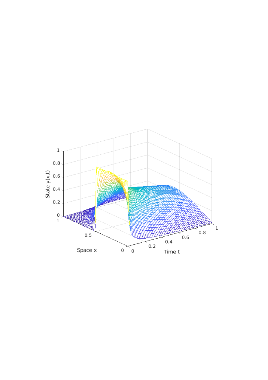
(a) State from initial control

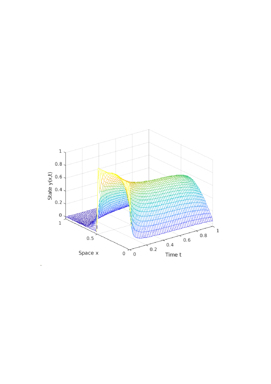
(b) Final iterate of gradient descent

(c) Final iterate of Gauss-Newton

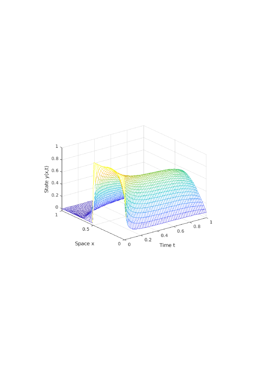
(d) Final iterate of Gauss-Newton+CG

Figure 1: State values for the optimal control problem (43) using $\nu=0.1$. The first plot shows the state for the initial value of the control, while the others show the state for the control returned by the corresponding variant of Algorithm 2.

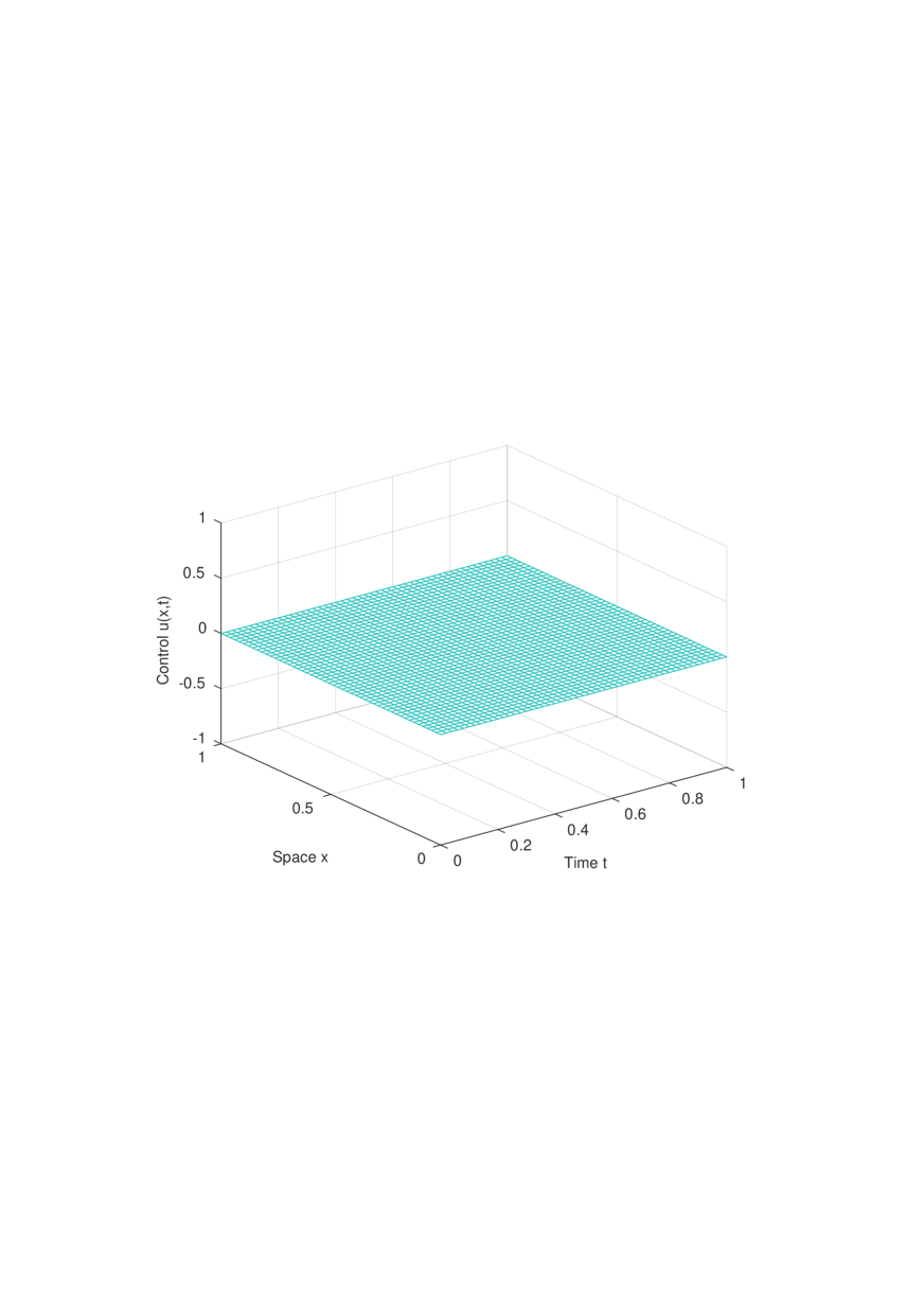
(a) Initial control

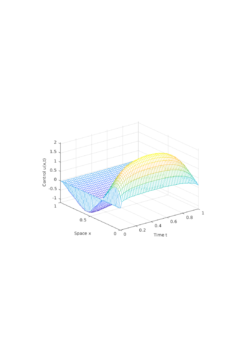
(b) Final control for gradient descent

(c) Final control for Gauss-Newton

(d) Final control for Gauss-Newton+CG

Figure 2: Control values for the optimal control problem (43) using $\nu=0.1$. The first plot shows the initial control value, while the others show the control returned by the corresponding variant of Algorithm 2.

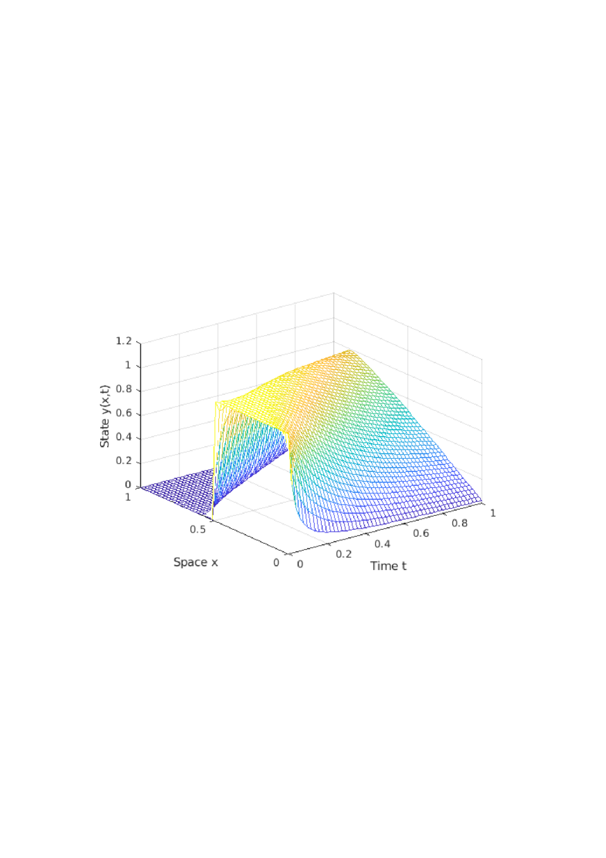
(a) State from initial control

(b) Final iterate of gradient descent

(c) Final iterate of Gauss-Newton

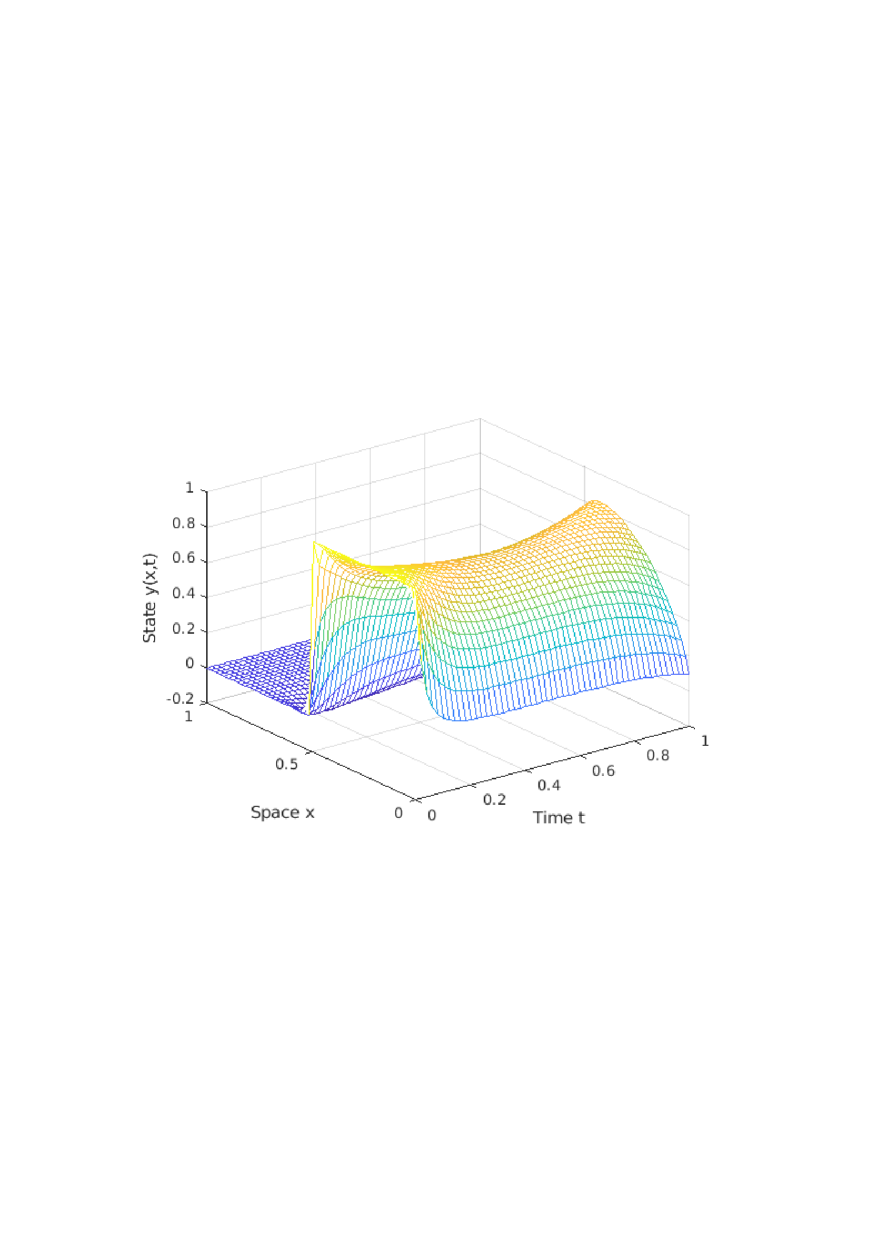
(d) Final iterate of Gauss-Newton+CG

Figure 3: State values for the optimal control problem (43) using $\nu=0.01$. The first plot shows the state for the initial value of the control, while the others show the state for the control returned by the corresponding variant of Algorithm 2.

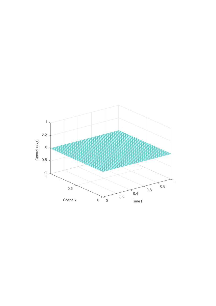
(a) Initial control

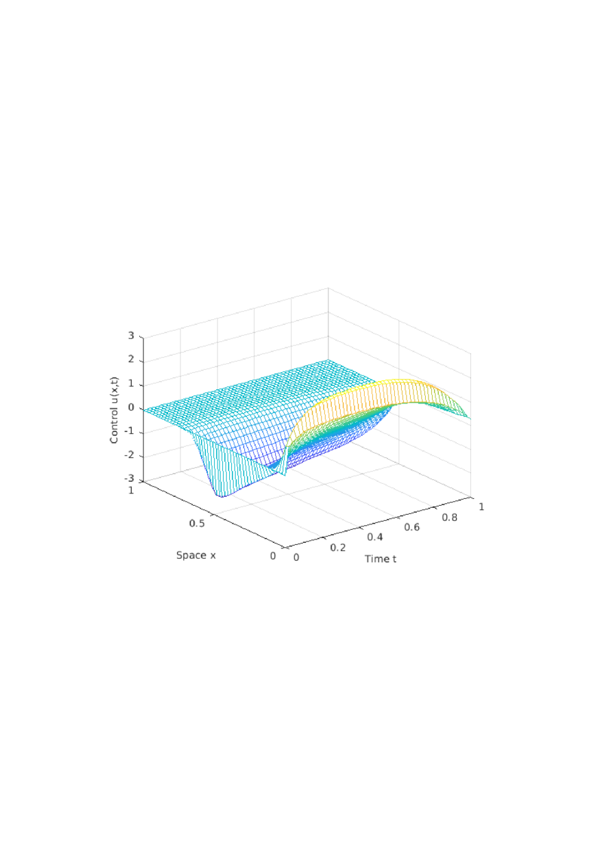
(b) Final control for gradient descent

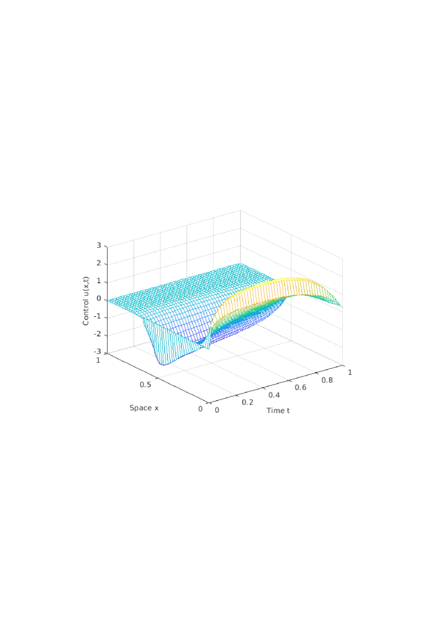
(c) Final control for Gauss-Newton

(d) Final control for Gauss-Newton+CG

Figure 4: Control values for the optimal control problem (43) using $\nu=0.01$. The first plot shows the initial control value, while the others show the control returned by the corresponding variant of Algorithm 2.

As illustrated by Table 4, the computation becomes more challenging as $\nu$ is smaller, since the instability grows exponentially with the evolution time [14]. Nevertheless, Figures 3 and 4 show that all three methods improve significantly over the state and the control compared to the initial control value. Note that the plot on the top left hand panel in Figure 1 and Figure 3 (resp. Figure 2 and Figure 4) represents the state corresponding to the initial control (resp. the initial control) while the other three plots in each figure represent the final iterate of the states (resp. the final control) computed with the respective variants of Algorithm 2.

5 Conclusion

In this paper, we proposed a regularization method for least-squares problems subject to implicit constraints, for which we derived complexity guarantees that improve over recent bounds derived in the absence of constraints. To this end, we leveraged a recently proposed convergence criterion that is particularly useful when the optimal solution corresponds to a nonzero objective value. Numerical testing conducted on PDE-constrained optimization problems showed that the criterion used to derive our complexity bounds bears a practical significance.

Our results can be extended in a number of ways. Deriving complexity results for second-order methods, that are common in scientific computing, is a natural continuation of our analysis. Besides, our study only considers deterministic operations. We plan on extending our framework to account for uncertainty in either the objective or the constraints, so as to handle a broader range of problems.

References

• [1] H. Antil, D. P. Khouri, M.-D. Lacasse, and D. Ridzal, editors. Frontiers in PDE-Constrained Optimization, volume 163 of The IMA Volumes in Mathematics and its Applications. Springer, New York, NY, USA, 2016.
• [2] M. M. Baumann. Nonlinear Model Order Reduction using POD/DEIM for Optimal Control of Burgers’ Equation. Master’s thesis, Faculty of Electrical Engineering, Mathematics and Computer Science Delft Institute of Applied Mathematics, Delft University of Technology, 2013.
• [3] E. Bergou, Y. Diouane, and V. Kungurtsev. Convergence and complexity analysis of a Levenberg-Marquardt algorithm for inverse problems. J. Optim. Theory Appl., 185:927–944, 2020.
• [4] E. Bergou, Y. Diouane, V. Kungurtsev, and C. W. Royer. A stochastic Levenberg-Marquardt method for using random models with complexity results and application to data assimilation. SIAM/ASA J. Uncertain. Quantif., 10:507–536, 2022.
• [5] C. Cartis, N. I. M. Gould, and Ph. L. Toint. On the evaluation complexity of cubic regularization methods for potentially rank-deficient nonlinear least-squares problems and its relevance to constrained nonlinear optimization. SIAM J. Optim., 23(3):1553–1574, 2013.
• [6] C. Cartis, N. I. M. Gould, and Ph. L. Toint. Evaluation Complexity of Algorithms for Nonconvex Optimization: Theory, Computation and Perspectives, volume MO30 of MOS-SIAM Series on Optimization. SIAM, 2022.
• [7] F. E. Curtis, D. P. Robinson, C. W. Royer, and S. J. Wright. Trust-region Newton-CG with strong second-order complexity guarantees for nonconvex optimization. SIAM J. Optim., 31:518–544, 2021.
• [8] J. C. de los Reyes and K. Kunisch. A comparison of algorithms for control constrained optimal control of the burgers equation. CALCOLO, 41:203 – 225, 2001.
• [9] H. Elman, D. Silvester, and A. Wathen. Finite Elements and Fast Iterative Solvers, volume Second Edition. Oxford University Press, 2014.
• [10] N. I. M. Gould, T. Rees, and J. A. Scott. A higher order method for solving nonlinear least-squares problems. Technical Report RAL-TR-2017-010, STFC Rutherford Appleton Laboratory, 2017.
• [11] N. I. M. Gould, T. Rees, and J. A. Scott. Convergence and evaluation-complexity analysis of a regularized tensor-Newton method for solving nonlinear least-squares problems. Comput. Optim. Appl., 73:1–35, 2019.
• [12] M. Heinkenschloss. Lecture notes CAAM 454 / 554 – Numerical Analysis II. Rice University, Spring 2018.
• [13] M. Hinze, R. Pinnau, M. Ulbrich, and S. Ulbrich. Optimization with PDE Constraints. Springer Dordrecht, 2009.
• [14] N. C. Nguyen, G. Rozza, and A. T. Patera. Reduced basis approximation and a posteriori error estimation for the time-dependent viscous Burgers’ equation. Calcolo, 46:157–185, 2009.
• [15] J. Nocedal and S. J. Wright. Numerical Optimization. Springer Series in Operations Research and Financial Engineering. Springer-Verlag, New York, second edition, 2006.
• [16] C. W. Royer and S. J. Wright. Complexity analysis of second-order line-search algorithms for smooth nonconvex optimization. SIAM J. Optim., 28:1448–1477, 2018.
• [17] L. Ruthotto and E. Haber. Deep neural networks motivated by partial differential equations. J. Math. Imaging Vision, 62:352–364, 2020.
• [18] F. Troeltzsch. Optimal Control of Partial Differential Equations: Theory, Methods and Applications. American Mathematical Society, 2010.
• [19] F. Troeltzsch and S. Volkwein. The SQP method for the control constrained optimal control of the Burgers equation. ESAIM: Control, Optimisation and Calculus of Variations, 6:649 – 674, 2001.
• [20] M. Ulbrich. Semismooth Newton Methods for Variational Inequalities and Constrained Optimization Problems in Function Spaces, volume MO11 of MOS-SIAM Series on Optimization. SIAM, 2011.