Riemannian Optimistic Algorithms

Abstract

In this paper, we consider Riemannian online convex optimization with dynamic regret. First, we propose two novel algorithms, namely the Riemannian Online Optimistic Gradient Descent (R-OOGD) and the Riemannian Adaptive Online Optimistic Gradient Descent (R-AOOGD), which combine the advantages of classical optimistic algorithms with the rich geometric properties of Riemannian manifolds. We analyze the dynamic regrets of the R-OOGD and R-AOOGD in terms of regularity of the sequence of cost functions and comparators. Next, we apply the R-OOGD to Riemannian zero-sum games, leading to the Riemannian Optimistic Gradient Descent Ascent algorithm (R-OGDA). We analyze the average iterate and best-iterate of the R-OGDA in seeking Nash equilibrium for a two-player, zero-sum, g-convex-concave games. We also prove the last-iterate convergence of the R-OGDA for g-strongly convex-strongly concave problems. Our theoretical analysis shows that all proposed algorithms achieve results in regret and convergence that match their counterparts in Euclidean spaces. Finally, we conduct several experiments to verify our theoretical findings.

1 Introduction

Online optimization has become increasingly important in recent decades, as it aims to optimize a sequence of decision variables in real-time, despite uncertainty and limited feedback. The online optimization has numerous applications in fields such as machine learning, signal imaging, and control systems [2, 24, 9].

The decision variables in online learning may be defined on Riemannian manifolds. Modeling signals on Riemannian manifolds can enhance data representation capabilities [40] and reduce problem dimension [38, 28]. Moreover, Riemannian optimization benefits from the property of geodesic convexity (g-convexity) [6], which permits conversion of Euclidean non-convex optimization problems into g-convex ones by appropriately choosing the Riemannian metric on the manifold. In this paper, we focus on the Riemannian online convex optimization (R-OCO) problem, defined as:

$$\min_{x_{t}\in\mathcal{K}\subset\mathcal{M}}\mathbf{f}_{t}(x_{t}),$$ (1)

where a learner plays against an adversary or nature. In each round $t\in 1,2,\dots,T$, the learner selects an action $x_{t}$ from a geodesically convex (g-convex) subset $\mathcal{K}$. The adversary or nature then produces a geodesically convex (g-convex) function $\mathbf{f}_{t}$ defined on $\mathcal{K}$ for which the learner has no prior knowledge. Finally, the learner receives feedback on $\mathbf{f}_{t}$ and incurs a corresponding loss $\mathbf{f}_{t}(x_{t})$. The problem (1) of Riemannian online convex optimization (R-OCO) is an extension of the classic online convex optimization in Euclidean spaces, with potential applications in machine learning, including robotic control, medical imaging, and neural networks [36, 19, 48].

In the context of the R-OCO problem, one important metric is the dynamic regret [31], which measures the difference in cumulative loss between an online optimization algorithm and a sequence of comparators $\{u_{1},\dots,u_{T}\}$, that is:

$${\sf{Reg}_{D}}(u_{1},\dots,u_{T})=\sum_{t=1}^{T}\mathbf{f}_{t}(x_{t})-\sum_{t=1}^{T}\mathbf{f}_{t}(u_{t}).$$

Compared to the well-known static regret [57]

$${\sf{Reg}_{S}}(T)=\sum_{t=1}^{T}\mathbf{f}_{t}(x_{t})-\min_{x\in\mathcal{M}}\sum_{t=1}^{T}\mathbf{f}_{t}(x),$$

the dynamic regret provides a more comprehensive evaluation of online algorithms, as it takes into account the adjustments and adaptations of the environment at each time step.

While it has been demonstrated that online convex optimization algorithms may result in $\Omega(T)$ dynamic regret bound in the worst case, it is also possible to bound dynamic regrets related to quantities that reflect the regularity of the problem [31, 54, 56], such as the path-length

$$P_{T}:=\sum_{t=2}^{T}d(u_{t},u_{t-1}),$$

the gradient variation

$$V_{T}:=\sum_{t=2}^{T}\sup_{x\in\mathcal{K}}\|\nabla\mathbf{f}_{t}(x)-\nabla\mathbf{f}_{t-1}(x)\|^{2},$$

and the comparator loss

$$F_{T}:=\sum_{t=1}^{T}\mathbf{f}_{t}(u_{t}).$$

If the comparators $u_{t}$ and the cost function $\mathbf{f}_{t}$ adapts slowly, the dynamic regret can be greatly reduced.

In Euclidean online convex optimization (OCO), the Online Optimistic Gradient Descent algorithm (OOGD)[31, 56] is a noteworthy example that certifies dynamic regret bounds based on path-length and gradient variation. The OOGD has been extensively studied and shown to achieve near-optimal dynamic regret bounds for a wide range of convex optimization problems. For instance, [31] presented a dynamic regret bound of $\mathcal{O}(P_{T}\sqrt{1+V_{T}})$ for the vanilla OOGD, and then [56] introduced a meta-expert structured OOGD that achieved a dynamic regret bound of $\mathcal{O}(\sqrt{(1+P_{T}+V_{T})(1+P_{T})})$. Moreover, the OOGD algorithm has also been applied to solve zero-sum games [44, 51, 22], which may be used to study generative adversarial networks [42].

Despite its success in Euclidean space, the extension of OOGD to Riemannian manifolds for dynamic regret has received limited attention. Some studies have examined the static regret of the R-OCO problem. [10] studied the static regret of Riemannian adaptive methods, which required a product manifold structure. [50] investigated the static regrets of the Riemannian online gradient descent algorithm and Riemannian online bandit methods.

With dynamic regrets, [41] explored a zeroth-order dynamic regret bound for strongly g-convex and strongly g-smooth functions on Hadamard manifolds. In recent works, [29] proposed several algorithms for adaptive dynamic regret bounds, incorporating gradient variation bounds, small loss bounds, and best-of-world bounds. In particular, [29] introduced the gradient variation regret bounds via a Riemannian extragradient algorithm framework. The extragradient framework, similar to optimistic algorithms, typically requires two gradients per iteration. One gradient is computed at the current decision point $x_{t}$, while the other gradient is obtained by extrapolating the current gradient to a midpoint $y_{t}$. However, it is worth noting that optimistic algorithms can operate solely based on the strategy point $x_{t}$. Thus, developing a Riemannian version of OOGD is crucial for advancing the field of online optimization on manifolds.

Contribution

Motivated by above, this paper aims to design optimistic online methods for Riemannian online optimization and derive dynamic regret bounds with respect to the regularity of the problem. The contribution of this paper is summarized as follows:

• We propose the Riemannian online optimistic gradient descent algorithm (R-OOGD), which uses only the gradient of the strategy point. We establish an $\mathcal{O}(P_{T}\sqrt{1+V_{T}})$ dynamic regret bound for g-convex losses.

• We introduce the meta-expert framework in [29] to the R-OOGD algorithm and propose the Riemannian online adaptive optimistic gradient descent (R-AOOGD) algorithm. We then establish a dynamic regret bound of $\mathcal{O}(\sqrt{(1+V_{T}+P_{T})(1+P_{T})})$ of the R-AOOGD on g-convex losses.

• We apply the R-OOGD algorithm to two-player zero-sum games on Riemannian manifolds and obtain the Riemannian Optimistic Gradient Descent Ascent algorithm (R-OGDA) for Nash equilibrium seeking in Riemannian zero-sum games. We prove $\mathcal{O}(\frac{1}{T})$ average-iterate and $\mathcal{O}(\frac{1}{\sqrt{T}})$ best-iterate convergence of the R-OGDA for g-convex-concave games. Moreover, we prove linear last-iterate convergence for g-strongly convex-strongly concave games.

The established regret bounds and convergence rates in our paper match the works in Euclidean space [31, 56, 43, 44]. We briefly list them in Table 1.

Algorithm	Problem setting	Result
R-OOGD	R-OCO, g-convex	$\mathcal{O}(\frac{\zeta_{0}}{\sqrt{\sigma_{0}}}P_{T}\sqrt{1+V_{T}})$
	Euclidean, convex	$\mathcal{O}(P_{T}\sqrt{1+V_{T}})$
		[31]
R-AOOGD	R-OCO, g-convex	$\mathcal{O}(\frac{\zeta_{0}}{\sqrt{\sigma_{0}}}\sqrt{(1+V_{T}+P_{T})(1+P_{T})})$
	Euclidean, convex	$\mathcal{O}(\sqrt{(1+V_{T}+P_{T})(1+P_{T})})$
		[56]
R-OGDA	RZS, g-convex-concave,	$\mathcal{O}(\frac{\zeta_{1}}{\sigma_{1}T})$
	average-iterate
	Euclidean convex-concave	$\mathcal{O}(\frac{1}{T})$
	average-iterate	[44]
	RZS, g-convex-concave	$\mathcal{O}(\frac{1}{\sqrt{\sigma_{1}}T})$
	best-iterate
	Euclidean convex-concave	$\mathcal{O}(\frac{1}{\sqrt{T}})$
	best-iterate	[14]
	RZS, g-SCSC, last-iterate	linear
	Euclidean, SCSC,	linear
	last-iterate	[43]

Table 1: Comparison of Algorithms in our work and corresponding Euclidean algorithms. SCSC denotes strongly convex-strongly concave. The constants $\zeta_{0},\zeta_{1},\sigma_{0},\sigma_{1}$ are related to Riemannian curvature and diameter bounds.

2 Related Work

In this section, we will provide a brief review of previous work on online convex optimization and zero-sum games in both Euclidean spaces and Riemannian manifolds.

2.1 Online Convex Optimization

Euclidean OCO

The concept of online optimization and static regret was introduced by [57]. [57] also proposed the online gradient descent (OGD) method and constructed an $\mathcal{O}(\sqrt{T})$ regret bound on convex functions. Later, [25] demonstrated that the OGD method achieves an $\mathcal{O}(\log T)$ regret bound on strongly convex functions. [1] proved the universal lower bounds for online algorithms to be $\Omega(\sqrt{T})$ and $\Omega(\log T)$ for convex and strongly convex functions respectively, which illustrated that the bounds of OGD are tight.

Aside from regret bounds related to the time horizon $T$, several papers explored the idea of exploiting regularity in the online optimization problem to achieve better regret bounds. For example, in addressing the online optimization problem where the loss functions have a small deviation, [17] proposed an online version of the extragradient algorithm, which achieved a regret bound of $\mathcal{O}(\sqrt{1+V_{T}})$ with respect to gradient variation $V_{T}:=\sum_{t=2}^{T}\sup_{x\in\mathcal{K}}\|\nabla\mathbf{f}_{t}(x)-\nabla\mathbf{f}_{t-1}(x)\|^{2}$ on convex and smooth functions. The online extragradient algorithm required constructing two gradients per iteration. To improve upon the extragradient algorithm, [46] proposed an online optimistic gradient descent (OOGD) method. The OOGD algorithm was also proved to achieve $\mathcal{O}(\sqrt{1+V_{T})}$ regret bounds by requiring only one gradient per iteration, which is suitable for one-point gradient feedback.

For the dynamic regret, [57] established a dynamic regret bound of $\mathcal{O}((1+P_{T})\sqrt{T})$ for the OGD algorithm, and [31] derived a dynamic regret bound of $\mathcal{O}(P_{T}\sqrt{1+V_{T}})$ for the OOGD algorithm. However, there is still a gap between these results and the universal lower dynamic regret bound of $\Omega(\sqrt{(1+P_{T})T})$ mentioned by [54]. To address this issue, [54] introduced a meta-expert framework to the OGD algorithm, which led to an optimal dynamic regret bound of $\mathcal{O}(\sqrt{(1+P_{T})T})$. Building upon the work of [54], [56] applied the meta-expert framework to the OOGD algorithm using a novel Online Optimistic Hedge technique in the meta-algorithm and obtained a gradient-variation bound $\mathcal{O}(\sqrt{(1+V_{T}+P_{T})(1+P_{T})})$, a small-loss bound $\mathcal{O}(\sqrt{(1+F_{T}+P_{T})(1+P_{T})})$, and a best-of-both-worlds bound $\mathcal{O}(\sqrt{(1+\min(V_{T},F_{T})+P_{T})(1+P_{T})})$ in Euclidean space. In this paper, the proposed R-OOGD algorithm and the R-AOOGD algorithm extend the results of the above Euclidean online optimistic algorithms to Riemannian manifolds beyond the restriction of linear structure.

Riemannian OCO

Riemannian optimization has garnered significant interest from researchers in the past few decades [53, 3, 10]. In the context of Riemannian online convex optimization, [8] introduced a regularized method that leverages the Riemann–Lipschitz continuity condition, which specifically targeted convex functions in an ambient Euclidean space. Furthermore, [10] provided regret analysis for Riemannian versions of the Adagrad and Adam algorithms, which relied on a product manifold structure. Later on, [41] proposed a Riemannian online zeroth-order algorithm and analyzed the dynamic regret bound of $\mathcal{O}(\sqrt{T}+P_{T}^{*})$ in the setting of g-strongly convex and g-smooth functions on Hadamard manifolds. Here, $P_{T}^{*}$ represents the length of the path between the optimal solutions $P_{T}^{*}:=\sum_{t=2}^{T}d(x_{t}^{*},x_{t+1}^{*})$. [50] proposed Riemannian online gradient methods with a sublinear static regret of $\mathcal{O}(\sqrt{T})$ in the full information setting, $\mathcal{O}(T^{2/3})$ in the one-point bandit information setting, and $\mathcal{O}(\sqrt{T})$ in the two-point bandit information setting for g-convex functions. In this paper, the dynamic regret bound of the proposed R-OOGD algorithm holds for geodesically convex functions on general manifolds and achieves a better static regret $\mathcal{O}(\sqrt{1+V_{T}})$ than the above mentioned results.

A recent breakthrough in understanding dynamic regret for Riemannian OCO was made by [29]. [29] first established a lower bound $\mathcal{O}(\sqrt{(1+P_{T})T})$ for minimax dynamic regrets for the Riemannian OCO. Then, [29] utilized the Fréchet mean and proposed a Riemannian meta-expert structure into the R-OGD, effectively achieving the universal lower bound for minimax dynamic regret. Additionally, [29] enhanced the meta-algorithm by incorporating Optimistic Hedge methods into Riemannian manifolds, which lead to a gradient-variation regret bound $\mathcal{O}(\sqrt{(1+V_{T}+P_{T})(1+P_{T})})$, a small-loss regret bound $\mathcal{O}(\sqrt{(1+F_{T}+P_{T})(1+P_{T})})$, and a best-of-both-worlds regret bound $\mathcal{O}(\sqrt{(1+\min(V_{T},F_{T})+P_{T})(1+P_{T})}+\min(V_{T},F_{T})\log T)$. Moreover, [29] also extended the regret bounds to the constrained setting using improper learning techniques. In order to obtain gradient-related dynamic regret bounds, [29] proposed the RADRv algorithm, which utilizes an extragradient-type algorithm (referred to as R-OCEG) as expert algorithm. The main insight of the R-OCEG algorithm is the extrapolation step, where the gradient of the current strategy point is used to extrapolate and obtain a midpoint. The current strategy point is then updated based on the gradient of the extrapolated point. As a result, the R-OCEG algorithm requires two gradient information in each iteration. In contrast, our R-OOGD algorithm does not rely on gradient extrapolation. Instead, the R-OOGD combines the gradient at the current decision point with parallel transported gradients from past decision points to perform update. The approach that parallel transporting past gradients allows our R-OOGD algorithm to achieve the same dynamic regret bound of $\mathcal{O}(P_{T}\sqrt{1+V_{T}})$ as the R-OCEG, while requiring only one round of gradient computations each turn. Furthermore, compared to the RADRv, our R-AOOGD algorithm, which employs the R-OOGD as the expert algorithm, achieves the same dynamic regret bound of $\mathcal{O}(\sqrt{(1+V_{T}+P_{T})(1+P_{T})})$ while utilizing half of the gradient information.

2.2 Optimistic algorithm in zero-sum games

ODGA in Euclidean zero-sum games

The Extragradient (EG) and Optimistic Gradient Descent Ascent (OGDA) methods have been extensively researched in the field of finding Nash equilibrium of Euclidean zero-sum games since the work of [34]. In the unconstrained convex-concave setting, both the EG and the OGDA methods exhibited $\mathcal{O}(1/T)$ average convergence rates, e.g., [e.g., 44]. [14] and [22] proved $\mathcal{O}(1/\sqrt{T})$ best-iterate convergence rates. In the constrained convex-concave setting, a more recent study by [12] demonstrated an $\mathcal{O}(1/\sqrt{T})$ last-iterate convergence rate of the OGDA. For the strongly convex-strongly concave setting, [43] demonstrated linear last-iterate convergence for both the OGDA and EG methods. Furthermore, [51, 22] extended this linear convergence rate to the constrained setting. In this paper, we propose a Riemannian extension of the OGDA method which preserves the average iterate and best-iterate convergence rate for g-convex-concave games, and linear last-iterate for g-strongly convex-strongly concave games.

Riemannian zero-sum games

Algorithms for coomputing the Nash equilibria (NE) in Riemannian zero-sum (RZS) games on Riemannian manifolds have been developed in the work of [37, 49, 20]. [30] introduced a Riemannian gradient descent ascent algorithm for RZS games where the second variable $y$ lied in a Euclidean space. [55] presented the Riemannian Corrected Extragradient algorithm (RCEG), which computes two gradients in one iteration and achieves $\mathcal{O}(\frac{1}{T})$ average-iteration convergence. Furthermore, for non-smooth functions, [32] presented $\mathcal{O}(\frac{1}{T})$ average-iterate convergence in the g-convex-concave setting and linear last-iterate convergence in the g-strongly-convex strongly-concave setting using Riemannian gradient descent ascent. [32] also constructed linear last-iterate convergence of the RCEG in the strongly g-convex setting. [23] introduced Riemannian Hamiltonian methods (RHM) that use the second-order Riemannian Hessian operator and established linear last-iterate convergence when the gradient norm of the payoff function satisfies the Riemannian Polyak–Łojasiewicz (PL) condition. In contrast, our ROGDA algorithm uses first-order information only once in each iteration and achieves the same average-iterate and last-iterate convergence. Moreover, our ROGDA algorithm shows the first best-iterate convergence result for g-convex-concave setting.

3 Preliminaries

Riemannian geometry

A Riemannian manifold $(\mathcal{M},g)$ is a manifold $\mathcal{M}$ with a point-varying Riemannian metric $g$. The Riemannian metric $g$ induces an inner product $\langle u,v\rangle_{x}=g_{x}(u,v)$ on every tangent space $T_{x}\mathcal{M}$. Via the inner product, notions of geometry can be brought onto Riemannian manifolds. For example, the norm of $u\in T_{x}\mathcal{M}$ is defined as $\|u\|=\sqrt{\langle u,u\rangle_{x}}$, the angle between $u,v\in T_{x}\mathcal{M}$ is $\arccos\frac{\langle u,v\rangle_{x}}{\|u\|\|v\|}$, and the length of a curve $\gamma:[0,1]\to\mathcal{M}$ is defined as $\int_{0}^{1}\|\dot{\gamma}(t)\|dt$.

A Riemannian manifold $\mathcal{M}$ also enjoys a metric space structure with distance $d(x,y)$, which is the minimum of the lengths of the curves connecting $x$ and $y$. A curve $\gamma$ is called a geodesic if it locally reaches the minimum length. An exponential map $\exp_{x}$ acts as a vector addition on Riemannian manifolds, which maps a tangent vector $v\in T_{x}\mathcal{M}$ to the endpoint $\gamma(1)$ of a geodesic $\gamma$ with the initial tangent vector $v$. Parallel transport $\Gamma_{\gamma}$ along the curve $\gamma$ translates vectors from one tangent space to another while preserving the inner product, i.e., $\langle u,v\rangle=\langle\Gamma_{\gamma}u,\Gamma_{\gamma}v\rangle$. In particular, we denote $\Gamma_{x}^{y}$ as the parallel transport along the geodesic between $x$ and $y$. The parallel transport determines the covariant derivative of the vector field $X$ along the vector field $Y$, which is defined as $\nabla_{X}Y(x)=\lim_{t\to 0}\frac{1}{t}\big{(}\Gamma_{\gamma}X(\gamma(t))-X(x)\big{)}$, where $\dot{\gamma}(0)=Y(x)$.

One of the most important notions in Riemannian geometry is the curvature tensor, defined as

$$R(X,Y,W,Z):=\langle\nabla_{X}\nabla_{Y}Z-\nabla_{Y}\nabla_{X}Z-\nabla_{[X,Y]}Z,W\rangle.$$

The sectional curvature is defined as $\frac{R(X,Y,X,Y)}{|X|^{2}|Y|^{2}-\langle X,Y\rangle^{2}}$ and characterizes the non-flatness of a $2$-dimensional Riemannian submanifold. On manifolds with non-positive sectional curvature, geodesics at one point $x$ spread away from each other so that the inverse exponential map $\exp^{-1}_{x}$ can be defined globally, while on manifolds with positive sectional curvature $K$, geodesics at one point gather with each other, making the inverse exponential map well-defined only in a neighborhood of $x$ with diameter less than $\frac{\pi}{\sqrt{K}}$. On the domain where the inverse exponential map is well-defined, we can write the distance function as $d(x,y)=\|\exp^{-1}_{x}y\|$.

Function classes

We introduce some function classes on Riemannian manifolds for the further analysis. First, we introduce the concept of geodesic convexity on Riemannian manifolds. A function $\mathbf{f}$ is considered to be geodesically convex (or g-convex) on $\mathcal{K}$, if for any $x$ and $y$ belonging to $\mathcal{K}$, it satisfies

$$\mathbf{f}(y)\geq\mathbf{f}(x)+\langle\nabla\mathbf{f}(x),\exp^{-1}_{x}y\rangle.$$

A function $\mathbf{f}$ is said to be $\mu$-strongly geodesically convex (or $\mu$-strongly g-convex) on $\mathcal{K}$, if for any $x$ and $y$ belonging to the manifold $\mathcal{M}$, the following inequality holds

$$\mathbf{f}(y)\geq\mathbf{f}(x)+\langle\nabla\mathbf{f}(x),\exp^{-1}_{x}y\rangle+\frac{\mu}{2}d^{2}(x,y).$$

Strong g-convexity also implies that

$$\langle-\nabla\mathbf{f}(x),\exp^{-1}_{x}x^{*}\rangle\geq\frac{\mu}{2}d^{2}(x,x^{*}),\quad\forall x\in\mathcal{M},$$

where $x^{*}$ is the global minimizer. Furthermore, a function $\mathbf{f}:\mathcal{K}\to\mathbb{R}$ is called geodesically concave (g-concave) if $-\mathbf{f}$ is g-convex and a function $\mathbf{f}:\mathcal{M}\to\mathbb{R}$ is called $\mu$-strongly geodesically concave ($\mu$-strongly g-concave) if $-\mathbf{f}$ is $\mu$-strongly g-convex.

We now define Lipschitz functions and smooth functions on Riemannian manifolds. We define a function $\mathbf{f}:\mathcal{M}\to\mathbb{R}$ as geodesically $G$-Lipschitz (or g-$G$-Lipschitz) if there exists a constant $G>0$ such that, for any $x,x^{\prime}\in\mathcal{M}$, the inequality $|\mathbf{f}(x)-\mathbf{f}(x^{\prime})|\leq G\cdot d(x,x^{\prime})$ holds. In the case of differentiable functions, this condition is equivalent to $\|\nabla\mathbf{f}(x)\|\leq G$ for all $x\in\mathcal{M}$. Similarly, a function $\mathbf{f}:\mathcal{M}\to\mathbb{R}$ is referred to as geodesically $L$-smooth if the gradient of $f$ satisfies the g-$L$-Lipschitz property, meaning that for any $x,x^{\prime}\in\mathcal{M}$, we have $\|\nabla\mathbf{f}(x)-\Gamma_{x^{\prime}}^{x}\nabla\mathbf{f}(x^{\prime})\|\leq L\cdot d(x,x^{\prime})$.

We now shift our focus to bivariate functions within the context of Riemannian zero-sum games. We call a bivariate function $\mathbf{f}(x,y):\mathcal{M}\times\mathcal{N}\to\mathbb{R}$ g-convex-concave (or $\mu$-g-strongly convex-strongly concave), if for every $(x,y)\in\mathcal{M}\times\mathcal{N}$, $\mathbf{f}(\cdot,y):\mathcal{M}\to\mathbb{R}$ is g-convex (or $\mu$-strongly g-convex) and $\mathbf{f}(x,\cdot):\mathcal{N}\to\mathbb{R}$ is g-concave (or $\mu$-strongly g-concave).

4 Riemannian Online Optimization with Dynamic Regret

In this section, we first introduce the Riemannian online optimistic gradient descent algorithm (R-OOGD) and the Riemannian adaptive online optimistic gradient descent algorithm (R-AOOGD), which aims to improve the dynamic regret bound by averaging $N$ R-OOGD algorithms with different step sizes. Then, we analyze the dynamic regret bounds of the R-OOGD and the R-AOOGD under g-convex functions.

4.1 Riemannian Online Optimistic Gradient Descent Method

The proposed R-OOGD algorithm is described in Algorithm 1. At each iteration $t$, the algorithm collects the gradient $\nabla\mathbf{f}_{t}(x_{t})$ and combines it with additional momentum

$$\nabla\mathbf{f}_{t}(x_{t})-\Gamma_{x_{t}-1}^{x_{t}}\nabla\mathbf{f}_{t-1}(x_{t-1}).$$

This combined gradient is then used in a gradient descent step via the exponential map $\exp_{x_{t}}$. The R-OOGD algorithm extends the Euclidean optimistic framework [43] to Riemannian manifolds.

Algorithm 1 Riemannian Optimistic Gradient Descent Algorithm (R-OOGD)

Manifold $\mathcal{M}$, step size $\eta$

Initialize $x_{-1}=x_{0}=x_{1}\in\mathcal{M}$.

for $t$ = $1$ to $T-1$ do

     Play $x_{t}$ and receive $\nabla\mathbf{f}_{t}(x_{t})$.

     Update $x_{t+1}=\exp_{x_{t}}(-2\eta\nabla\mathbf{f}_{t}(x_{t})+\eta\Gamma^{x_{t}}_{x_{t-1}}\nabla\mathbf{f}_{t-1}(x_{t-1}))$

end for

Sequence $(x_{t})_{t=1}^{T}$.

Next, inspired by [29], we introduce a meta-expert framework to the R-OOGD. We propose the Riemannian adaptive online optimistic gradient descent algorithm (R-AOOGD) in Algorithms 2 and 3.

Algorithm 2 R-AOOGD: Meta Algorithm

1:Manifold $\mathcal{M}$, learning rate $\beta$, step size pool $\mathcal{H}={\eta_{i};i=1,2,\dots,N}$ and parameters $K,\alpha$.

2:Initialize $x_{0}\in\mathcal{M}$. Set initial weights $w_{0,1}=w_{0,2}=\dots=w_{0,N}=1/N$.

3:for $t=1$ to $T$ do

4:     Receive $x_{i,t}$ from $N$ expert algorithms with step size $\eta_{i}$.

5:     Set $\bar{x}_{t}=\arg\min_{x}w_{t-1,i}d^{2}(x,x_{t,i})$

6:     Update $w_{t,i}\propto e^{\big{(}-\beta(\sum_{j=1}^{t-1}l_{i,j}+m_{i,t})\big{)}}$ by

$$\begin{cases}l_{i,t}=\langle\nabla\mathbf{f}_{t}(x_{t}),\exp^{-1}_{x_{t}}x_{i,t}\rangle\\ m_{i,t}=\langle\nabla\mathbf{f}_{t}(\bar{x}_{t}),\exp^{-1}_{\bar{x}_{t}}x_{i,t}\rangle\\ \end{cases}$$

7:     Set $x_{t}=\arg\min_{x}w_{t,i}d^{2}(x,x_{t,i})$.

8:end for

9:return $\{x_{t}\}_{t=1}^{T}$.

Algorithm 3 R-AOOGD: Expert Algorithm

Manifold $\mathcal{M}$, feasible set $\mathcal{K}$ and step size $\eta_{i}$ from the pool $\mathcal{H}$.

Initialize $x_{i,-1}=x_{i,0}=x_{i,1}\in\mathcal{K}$.

for $t$ = $1$ to $T-1$ do

     Send $x_{i,t}$ to the meta algorithm.

     Update $x_{i,t+1}=\exp_{x_{i,t}}(-2\eta_{i}\nabla\mathbf{f}_{t}(x_{i,t})+\eta_{i}\Gamma^{x_{i,t}}_{x{i,t-1}}\nabla\mathbf{f}_{t-1}(x_{i,t-1}))$.

end for

4.2 Dynamic Regret Analysis

In order to analyze the regret bounds of the R-OOGD and the R-AOOGD, we impose some assumptions, which are standard in the literature of online learning and Riemannian optimization [8, 44, 43, 3, 5].

Assumption 1.

The function $\mathbf{f}_{t}$ is g-convex, g-$G$-Lipschitz, and g-$L$-smooth over the set $\mathcal{K}\subset\mathcal{M}$.

The following two assumptions focus on the geometry of the manifolds $\mathcal{M}$.

Assumption 2.

All sectional curvatures of $\mathcal{M}$ are bounded below by a constant $\kappa$ and bounded above by a constant $K$.

Assumption 3.

The diameter of the feasible set $\mathcal{K}$ is bounded by $D_{0}$. If $K>0$, the diameter $D_{0}$ is less than $\frac{\pi}{2\sqrt{K}}$.

Assuming boundedness of the feasible set is a fundamental setting in online optimization algorithms [57, 1, 56], while the additional constraint $D_{0}\leq\frac{\pi}{2\sqrt{K}}$ is also a common condition adopted in the literature of Riemannian optimization on positively curved manifolds [53, 5, 55]. Assumption 3 ensures that there are no conjugate points on $\mathcal{K}$ according to the conjugate point theorem [35], guaranteeing that the inverse exponential map $\exp^{-1}_{x}(\cdot)$ can be defined throughout $\mathcal{K}$. Additionally, the Hessian comparison theorem [35] indicates that when the diameter of $\mathcal{K}$ is greater than $\frac{\pi}{\sqrt{K}}$, the subset $\mathcal{K}$ may be “infinitely curved,” meaning that the Hessian of the distance function $d(x,\cdot)$ may blow up. As in Riemannian optimization, we usually bound the loss by the g-convexity, i.e.,

$$\mathbf{f}_{t}(x_{t})-\mathbf{f}_{t}(u_{t}) \leq\langle\nabla\mathbf{-}\mathbf{f}_{t}(x_{t}),\exp^{-1}_{x_{t}}u_{t}\rangle=\langle\nabla\mathbf{f}_{t}(x_{t}),\nabla_{x_{t}}(\frac{1}{2}d^{2}(x_{t},u_{t}))\rangle,$$

and then use the Hessian of the distance function $d(x,u_{t})$ for further analysis.

We also note that Assumption 3 does not necessarily affect the applicability of the proposed algorithms in practical problems. Our experiments (see Subsection 6.2) demonstrate that a feasible set $\mathcal{K}$ with a much larger diameter than $\frac{\pi}{2\sqrt{K}}$ (even the whole manifold $\mathcal{M}$) does not significantly affect the performance of our proposed algorithms.

We impose the following assumption on invariance of the set $\mathcal{K}$ during the execution of Algorithm 1. The same assumption has also been used in the work by [3, 5, 55]. In addition, and we do not observe the assumption to be violated in our experiments.

Assumption 4.

All iterations of Algorithms 1 lie in the set $\mathcal{K}$.

Now we begin to analyze regret bounds. Our analysis heavily relies on comparison inequalities [53, 5], which enable us to quantify the distortion by nonlinear structure with respect to the curvature bound $\kappa$, $K$ and domain diameter $D_{0}$. Specially, we can bound the minimum and maximum distortion rates by two parameters

$$\sigma(K,D)=\begin{cases}\frac{\sqrt{K}D}{\tan(\sqrt{K}D)}&K>0;\\ 1&K\leq 0,\end{cases}\quad\text{and}\quad\zeta(\kappa,D)=\begin{cases}\frac{\sqrt{-\kappa}D}{\tanh(\sqrt{-\kappa}D)}&\kappa<0;\\ 1&\kappa\geq 0.\end{cases}$$

After that, we can establish regret bounds for the R-OOGD algorithm.

4.2.1 Dynamic Regret for R-OOGD

Theorem 1.

Let $\sigma_{0}=\sigma(K,D_{0})$ and $\zeta_{0}=\zeta(\kappa,D_{0})$. Suppose that Assumptions 1-4 hold. Then, for the sequence $\{x_{t}\}_{t=1}^{T}$ generated by Algorithm 1 with step size $\eta\leq\frac{\sigma_{0}}{4\zeta_{0}L}$, the following inequality holds for an arbitrary sequence $\{u_{t}\}_{t=1}^{T}$:

$${\sf{Reg}_{D}}(u_{1},\dots,u_{T})\leq\frac{D_{0}^{2}+2D_{0}P_{T}}{\eta}+\eta\frac{4\zeta_{0}^{2}}{\sigma_{0}}(G^{2}+V_{T}),$$

where $P_{T}=\sum_{t=2}^{T}d(u_{t},u_{t-1})$ is the path-length, and $V_{T}=\sum_{t=2}^{T}\sup_{x\in\mathcal{K}}\|\nabla\mathbf{f}_{t}(x)-\nabla\mathbf{f}_{t-1}(x)\|^{2}$ is the gradient variation. If $V_{T}$ is known beforehand, the dynamic regret bound can be improved to $\mathcal{O}(P_{T}\sqrt{1+V_{T}})$.

Corollary 1.

Suppose that Assumptions 1-4 hold. Algorithm 1 incurs the static regret with the optimal step size $\eta^{*}=\min(\sqrt{\frac{D_{0}^{2}\sigma_{0}}{4\zeta_{0}^{2}(G^{2}+V_{T})}},\frac{\sigma_{0}}{4\zeta_{0}L})$,

$${\sf{Reg}_{S}}(T)\leq\mathcal{O}\big{(}\zeta_{0}\sqrt{\frac{1}{\sigma_{0}}(1+V_{T})}\big{)}.$$

The proofs of Theorem 1 and Corollary 1 are shown in Appendix B. In Theorem 1 and Corollary 1, we provide an $\mathcal{O}(P_{T}\sqrt{1+V_{T}})$ dynamic regret bound and an $\mathcal{O}(\sqrt{1+V_{T}})$ static regret bound for the R-OOGD, respectively. These bounds recover the corresponding work on online optimization in Euclidean space [31, 54, 56]. Compared to the extragradient-structured R-OCEG algorithm by [29] in the unconstrained setting, our method only requires one gradient information per iteration, making it less computationally demanding and more applicable to the one-point gradient feedback online learning model.

4.2.2 R-OOGD with Parallel Transport

Conversion of past gradients plays a vital role in designing Riemannian optimistic algorithms. Apart from the parallel transport method utilized in our R-OOGD algorithm, there is another methodology known as the correction term to transport past graident in Riemannian optimization [55, 29]. The correction term involves changing the base point of the exponential map to avoid parallel transport. Specifically, when considering two points $a$ and $b$, along with a tangent vector $v\in T_{a}\mathcal{M}$, the correction term employs $\exp_{a}(v+\exp_{a}^{-1}(b))$ instead of the direct parallel transport $\exp_{b}(\Gamma_{a}^{b}v)$. If our R-OOGD algorithm incorporates the correction term methodology, the algorithm will be expressed as follows,

$$\begin{cases}x_{t+1}=\exp_{x_{t}}(-2\eta\nabla\mathbf{f}_{t}(x_{t})+\exp^{-1}_{x_{t}}\hat{x}_{t})\\ \hat{x}_{t+1}=\exp_{x_{t}}(-\eta\nabla\mathbf{f}_{t}(x_{t})+\exp^{-1}_{x_{t}}\hat{x}_{t}).\end{cases}$$ (2)

However, incorporating the correction term into our R-OOGD algorithm does not yield an efficient online algorithm and is unable to guarantee a sublinear static regret. This is because the correction term introduces distortion in the inner product, and these distortions grow unboundedly over time. To be more precise, in order to analyze the static regret bound, we need to estimate the distortion in the inner product between the correction term and the real gradient term

$$A_{t}:=\langle\exp^{-1}_{x_{t}}\hat{x}_{t}-\Gamma_{x_{t-1}}^{x_{t}}\eta\nabla\mathbf{f}_{t-1}(x_{t-1}),\exp^{-1}_{x_{t}}x\rangle$$

at each iteration. However, as demonstrated in Appendix C, the distortion bound $A_{t}$ depends on the previous distortion $A_{t-1}$, which is governed by the recursive formula:

$$A_{t}\leq\mathcal{O}\Big{(}(5\eta G+2A_{t-1})^{2}(3\eta G+A_{t-1})\Big{)}.$$ (3)

Therefore, the distortion accumulates iteratively and may eventually blow up. In contrast, our parallel transport method preserves the inner product, guaranteeing that the distortion term remains zero. Consequently, it is crucial to emphasize that parallel transporting past gradients is essential to ensure the effectiveness of the R-OOGD algorithm.

4.2.3 Dynamic Regret for R-AOOGD

Now we begin to analyze the the dynamic bound of the R-AOOGD algorithm.

Theorem 2.

Suppose that Assumptions 1-4 hold. Set $\mathcal{H}=\{\eta_{i}=2^{i-1}\sqrt{\frac{\sigma_{0}D_{0}^{2}}{16\zeta_{0}^{2}G^{2}T}}\}$, $N=\Big{\lceil}\frac{1}{2}\log_{2}\big{(}\frac{\sigma_{0}G^{2}T}{D_{0}^{2}L^{2}}\big{)}\Big{\rceil}+1$ and $\beta=\min\Big{(}\frac{1}{\sqrt{12D_{0}^{4}L^{2}+D_{0}^{2}G^{2}\zeta_{0}^{2}}},\sqrt{\frac{2+\ln N}{3D_{0}^{2}(V_{T}+G^{2})}}\Big{)}$. The R-AOOGD algorithm (Algorithms 2 and 3) incurs the dynamic regret

$${\sf{Reg}_{D}}(u_{1},\dots,u_{T})\leq\mathcal{O}\Big{(}\frac{\zeta_{0}}{\sqrt{\sigma_{0}}}\sqrt{(1+V_{T}+P_{T})(1+P_{T})}\Big{)}.$$

The proof of Theorem 2 can be found in Appendix B. In Theorem 2,An $\mathcal{O}\Big{(}\sqrt{(1+V_{T}+P_{T})(1+P_{T})}\Big{)}$ regret bound is established for our meta-expert algorithm R-AOOGD which aligns with the findings in online optimization in Euclidean space [56]. When considering the RADRv algorithm [29], which is another Riemannian online meta-expert algorithm, we observe certain differences compared to our R-AOOGD algorithm. In the non-projection case, the RADRv algorithm at the meta level requires $N=\Big{\lceil}\frac{1}{2}\log_{2}\big{(}\frac{4\sigma_{0}G^{2}T}{D_{0}^{2}L^{2}}\big{)}\Big{\rceil}+1$ expert algorithms, which is equal to or more than the number of experts required by our R-AOOGD algorithm. Additionally, at the expert level, the RADRv requires two gradients per iteration, while our R-AOOGD algorithm only requires one gradient. As a result, our R-AOOGD algorithm achieves the same order of regret bound of $\mathcal{O}\Big{(}\sqrt{(1+V_{T}+P_{T})(1+P_{T})}\Big{)}$ while utilizing only half the number of gradients.

5 Application: Nash Equilibrium Seeking in Riemannian Zero-sum Games

In this section, we apply our R-OOGD to Riemannian zero-sum (RZS) games, where both players update their actions based on the R-OOGD dynamics. We then analyze the convergence rates of the resulting Riemannian Optimistic Gradient Descent Ascent method (R-OGDA). Specifically, we study the average-iterate convergence rate and the best-iterate convergence rate for g-convex-concave games, as well as the last-iterate convergence rate for g-strongly convex-strongly concave games.

5.1 Formulation of Riemannian Zero-sum Games

Riemannian zero-sum (RZS) games involve a competitive scenario between two players, denoted as $\mathtt{X}$ and $\mathtt{Y}$, i.e.,

$$\min_{x\in\mathcal{M}}\max_{y\in\mathcal{N}}\mathbf{\mathbf{f}}(x,y),$$ (4)

where player-$\mathtt{X}$ tries to find a strategy $x$ from a Riemannian manifold $\mathcal{M}$ to minimize the payoff function $\mathbf{f}(x,y)$, while player-$\mathtt{Y}$ tries find a strategy $y$ from a Riemannian manifold $\mathcal{N}$ to maximize the payoff function $\mathbf{f}(x,y)$.

A key concept in the RZS games is Nash Equilibrium (NE). In the RZS game, an action pair $(x^{*},y^{*})\in\mathcal{M}\times\mathcal{N}$ is an NE if no player can improve individual payoff by only deviating his own action, i.e.,

$$\max_{y\in\mathcal{N}}\mathbf{f}(x^{*},y)=\mathbf{f}(x^{*},y^{*})=\min_{x\in\mathcal{M}}\mathbf{f}(x,y^{*}).$$

Computing NEs in the Riemannian zero-sum games has direct applications in several learning tasks including minimum balanced cut, robust geometry-aware PCA, and robust Wasserstein barycenters [33, 27, 39, 55].

5.2 Riemannian Optimistic Gradient Descent Ascent Algorithm

We propose the Riemannian Optimistic Gradient Descent Ascent Algorithm (R-OGDA) as follows.

Algorithm 4 Riemannian Optimistic Gradient Descent Ascent

$(\mathcal{M},\mathcal{N}$), step size $\eta$,

Initialize $(x_{-1},y_{-1})=(x_{0},y_{0})\in\mathcal{M}\times\mathcal{N}$.

for $t$ = $2$ to $T-1$ do

     Update $x_{t+1}=\exp_{x_{t}}(-2\eta\nabla_{x}\mathbf{f}(x_{t},y_{t})+\eta\Gamma^{x_{t}}_{x_{t-1}}\nabla_{x}\mathbf{f}(x_{t-1},y_{t-1}))$

     Update $y_{t+1}=\exp_{y_{t}}(2\eta\nabla_{y}\mathbf{f}(x_{t},y_{t})-\eta\Gamma^{y_{t}}_{y_{t-1}}\nabla_{y}\mathbf{f}(x_{t-1},y_{t-1}))$

     Average from geodesic

$$\begin{cases}\bar{x}_{t+1}=\exp_{\bar{x}_{t}}(\frac{1}{(t+1)}\exp^{-1}_{\bar{x}_{t}}x_{t+1})\\ \bar{y}_{t+1}=\exp_{\bar{y}_{t}}(\frac{1}{(t+1)}\exp^{-1}_{\bar{y}_{t}}y_{t+1})\end{cases}$$ (5)

end for

Sequence $(x_{t},y_{t})_{t=1}^{T}$, average $(\bar{x}_{T},\bar{y}_{T})$ .

5.3 Average-Iterate Analysis

We first analyze the convergence rate of averaged iterate $(\bar{x}_{T},\bar{y}_{T})$ by adpoting the following assumptions. To ease the notation, we denote $z_{t}=(x_{t},y_{t})$, $z^{*}=(x^{*},y^{*})$, and $\mathbf{F}(z_{t})=[\nabla_{x}\mathbf{f}(z_{t}),-\nabla_{y}\mathbf{f}(z_{t})]$.

Assumption 5.

The payoff function $f$ is g-$G$-Lipschitz and g-convex-concave on the manifold $\mathcal{M}\times\mathcal{N}$.

The g-convexity-concavity is helpful in analyzing Nash equilibriums. For any NE point $z^{*}=(x^{*},y^{*})$, the g-convexity-concavity of $\mathbf{f}$ implies that

$$\langle-\mathbf{F}(z),\exp^{-1}_{z}z^{*}\rangle\geq 0$$

holds for all $z\in\mathcal{M}$. Moreover, if $\mathbf{f}$ is $\mu$-g-strongly-convex strongly-concave, it further holds that for all $z\in\mathcal{M}$,

$$\langle-\mathbf{F}(z),\exp^{-1}_{z}z^{*}\rangle\geq\frac{\mu}{2}d^{2}(z,z^{*}).$$ (6)

Assumption 6.

The payoff function $f$ is g-$L$-smooth on $\mathcal{M}\times\mathcal{N}$, i.e., there is a constant $L>0$ such that

$$\|\nabla\mathbf{f}(x,y)-\Gamma_{(x^{\prime},y^{\prime})}^{(x,y)}\nabla\mathbf{f}(x^{\prime},y^{\prime})\|^{2}\leq L^{2}(d^{2}(x,x^{\prime})+d^{2}(y,y^{\prime})),\quad\forall(x,y),(x^{\prime},y^{\prime})\in\mathcal{M}\times\mathcal{N}.$$

Assumption 7.

There is a Nash equilibrium $z^{*}=(x^{*},y^{*})$ in the Riemannian zero-sum game (4).

Assumption 7 can be directly derived from the g-strongly convex-strongly concave property of $\mathbf{f}$ in certain cases. In the case where the manifold $\mathcal{M}$ is compact or the level set $\{(x,y)\mid-\infty\leq\mathbf{f}(x,y)\leq\infty\}$ is bounded, we can rely on the Riemannian analog of Sion’s minimax theorem [55] to establish the existence of a Nash equilibrium. Furthermore, if we assume g-strong-convexity strong-concavity of the function $\mathbf{f}$, by (6), Assumption 7 guarantees the uniqueness of the resulting Nash equilibrium $z^{*}$.

Assumption 8.

All sectional curvatures of $\mathcal{M}$ and $\mathcal{N}$ are bounded below by a constant $\kappa$ and bounded above by a constant $K$.

We first show that it is possible to drop the boundedness assumption (Assumption 3) in the iteration of $x_{t}$ and $y_{t}$ in the Riemannian zero-sum (RZS) games (4), if prior knowledge of the distance $d(z_{0},z^{*})$ is available. The following Lemma 1 ensures that the iteration of $x_{t}$ and $y_{t}$ is in a bounded set $\mathcal{K}$.

Lemma 1.

Suppose Assumptions 5-8 hold. Let the step size $\eta$ satisfying $\eta\leq\min(\frac{\sigma_{1}}{\zeta_{1}L},\frac{D_{1}}{3G})$. Let $d(z_{0},z^{*})\leq D_{1}<\frac{\pi}{6\sqrt{K}}$, then by denoting $\zeta_{1}=\zeta(\kappa,3D_{1})$ and $\sigma_{1}=\zeta(K,3D_{1})$, we have $d(z_{t},z^{*})\leq 2D_{1}$ for all iterations $t$.

Then we derive the average-iterate convergence rate for g-convex-concave RZS games in the following Theorem 3.

Theorem 3.

Under Assumptions 5-8 and the condition in Lemma 1, the averaged iterate $(\bar{x}_{T},\bar{y}_{T})$ of Algorithm 4 with the step size $\eta\leq\frac{\sigma_{1}}{2\zeta_{1}L}$ satisfies:

$$\max_{y\in\mathcal{N}}\mathbf{f}(\bar{x}_{T},y)-\min_{x\in\mathcal{M}}\mathbf{f}(x,\bar{y}_{T})\leq\frac{D_{1}^{2}L+\frac{D_{1}^{2}}{2\eta}}{T}$$

The proof of Theorem 3 is in Appendix D. Theorem 3 demonstrates that the averaged iterate $(\bar{x}_{T},\bar{y}_{T})$ is an $\mathcal{O}(\frac{1}{T})$-NE in g-convex-concave RZS games. The result extends the corresponding results in Euclidean spaces [43] and recovers the convergence rate of RCEG [55] by acquiring only one gradient in each iteration.

5.4 Last-Iterate/Best-Iterate Analysis

In this section, we focus on the last/best-iterate convergence of our R-OGDA algorithm. Dealing with the convergence of the R-OGDA algorithm in terms of the last-iterate or best-iterate is quite challenging. In Euclidean spaces, optimistic gradient descent/ascent algorithms benefit from the perspective of “extrapolation from the past” [21]. This means that by defining the immediate sequence

$$\hat{z}^{E}_{t+1}=z_{t}-\eta(\mathbf{F}(z_{t})+\mathbf{F}(z_{t-1})),$$ (*)

the relationship holds [21]:

$$\eta\mathbf{F}(z_{t})=\hat{z}^{E}_{t}-\hat{z}^{E}_{t+1}.$$ (**)

However, when we define the Riemannian counterparts of (*) ‣ 5.4 $\hat{z}_{t+1}=\exp_{z_{t}}(\eta(-\mathbf{F}(z_{t})+\mathbf{F}(z_{t-1})))$, it fails to hold that $\exp^{-1}_{\hat{z}_{t+1}}\hat{z}_{t}=\eta\Gamma_{z_{t}}^{\hat{z}_{t+1}}\mathbf{F}(z_{t})$, which is the Riemannian version of (**) ‣ 5.4. In addition, measuring the distortion between vector $\exp^{-1}_{\hat{z}_{t+1}}\hat{z}_{t}$ and $\eta\Gamma_{z_{t}}^{\hat{z}_{t+1}}\mathbf{F}(z_{t})$ is challenging.

One natural idea is to parallel transport the tangent vectors $\exp^{-1}_{z_{t}}z_{t-1}$, $\exp^{-1}_{z_{t}}\hat{z}_{t}$ and $\exp^{-1}_{z_{t+1}}\hat{z}_{t+1}$ to the tangent space at $\hat{z}_{t+1}$, and then estimate the distortion between $G_{t}$ and $\Gamma_{z_{t}}^{\hat{z}{t+1}}\mathbf{F}(z_{t})$ using their vector sum. A commonly used technique in manifold settings, the comparison inequalities [53, 5], follows the same idea to estimate the Hessian-type distortion, i.e.,

$$\sigma(K,D)\|\exp^{-1}_{a}b\|\leq\|\exp^{-1}_{a}b-\Gamma_{c}^{a}\exp^{-1}_{c}b\|\leq\zeta(k,D)\|\exp^{-1}_{a}b\|.$$

The crux of these inequalities is to use the gradient squared distance $\nabla d(b,x)=-\exp^{-1}_{b}x$ on the manifold, and then estimate the error by exploiting the eigenvalues of the Hessian matrix of the distance function. Therefore, the comparison inequalities require the compared tangent vectors to share the same endpoint, which is not applicable in our case.

Furthermore, we have observed that the distortion analysis between $G_{t}$ and $\Gamma_{z_{t}}^{\hat{z}{t+1}}\mathbf{F}(z_{t})$ brings in extra errors beyond the Hessian-type distortions. Parallel transporting vectors in the two distinct tangent spaces to a third tangent space can lead to additional distortion. Specifically, when dealing with three points $a,b,c$, and vectors $v\in T_{a}\mathcal{M}$ and $w\in T_{b}\mathcal{M}$, we have

$$\|\Gamma_{a}^{c}v-\Gamma_{b}^{c}w\|\neq\|\Gamma_{a}^{b}v-w\|.$$

In particular, it holds

$$\|\Gamma_{a}^{c}v-\Gamma_{b}^{c}w\|=\|\Gamma_{a}^{b}v-w\|+\|\Gamma_{b}^{a}\Gamma_{c}^{b}\Gamma_{a}^{c}v-w\|.$$

On Riemannian manifolds, the latter term $\|\Gamma_{b}^{a}\Gamma_{c}^{b}\Gamma_{a}^{c}v-w\|$ does not vanish due to the presence of the holonomy effects, which indicates that parallel transport around closed loops fails to preserve the geometric data being transported. Therefore, estimating the distortion between $G_{t}$ and $\Gamma_{z_{t}}^{\hat{z}{t+1}}\mathbf{F}(z_{t})$ is faced with the change of holonomy distortion and becomes highly nontrivial.

To address the aforementioned difficulties, we propose a key technique inspired by the famous Gauss-Bonnet theorem [16], and estimate the holonomy distortion by the step size $\eta$ and sectional curvature $K_{m}=\max\{|K|,|\kappa|\}$.

Lemma 2.

Suppose that $\mathbf{f}$ is g-$L$-smooth. If the step size $\eta\leq\frac{1}{20L}$, them $G_{t+1}=\exp^{-1}_{\hat{z}_{t+1}}\hat{z}_{t}$ satisfies the following

• $\|G_{t+1}\|^{2}-\|\eta\mathbf{F}(z_{t})\|^{2}\leq 64K_{m}^{2}\eta^{6}\|\mathbf{F}(z_{t-1})\|^{6}$;

• $\|\Gamma_{\hat{z}_{t+1}}^{z_{t}}G_{t+1}-\eta\mathbf{F}(z_{t})\|\leq 104K_{m}\eta^{3}\|\mathbf{F}(z_{t-1})\|^{3}$.

According to Lemma 2, the holonomy distortion turns out to be $\mathcal{O}(K_{m}\eta^{3})$, which enables us to obtain the convergence in Theorems 4 and 5. In the following theorems, we denote $\Upsilon=\frac{1}{5}\sigma_{1}L+\frac{28}{5}(\zeta_{1}-\sigma_{1})L+104(2D_{1}+\frac{1}{5})K_{m}G+8\sigma_{1}K_{m}G$.

Theorem 4.

Suppose Assumptions 5-8 and conditions in Lemma 1 hold. Algorithm 4 incurs the best-iterate convergence with the step size $\eta\leq\min\{\frac{1}{20L},\frac{1}{8G},\frac{\sigma_{1}}{2\Upsilon}\}$,

$$\min_{t\leq T}\|\nabla\mathbf{f}(z_{t})\|\leq\mathcal{O}(\frac{1}{\sqrt{T}}),$$

and moreover, we have $\lim_{t\to\infty}\|\nabla\mathbf{f}(z_{t})\|=0$.

Theorem 5.

Suppose Assumptions 5-8 and conditions in Lemma 1 hold and $\mathbf{f}$ is $\mu$-g-strongly convex-strongly concave. Recall $z^{*}$ is the unique NE of the game (4). Algorithm 4 with the step size
$\eta\leq\min\{\frac{1}{20L},\frac{1}{8G},\frac{\sigma_{1}}{\Upsilon+4\mu+8\sigma_{1}\mu}\}$ incurs

$$d^{2}(z_{t},z^{*})\leq\Big{(}\frac{1}{1+\eta\mu/2}\Big{)}^{t}\big{(}2(1+\frac{1}{\sigma_{1}})d^{2}(z_{1},z^{*})\big{)}.$$

The proofs for Theorems 4 and 5 can be found in Appendix F. Theorem 4 demonstrates the $\mathcal{O}(\frac{1}{\sqrt{T}})$ convergence rate for the best iterate of g-convex-concave games, which is the first proven result in Riemannian NE seeking algorithms for g-convex-concave games. Moreover, Theorem 5 establishes a linear convergence rate for the last-iterate of the ROGDA algorithm, matching those in the RCEG algorithm and the second-order RHM algorithm [23, 32] in the g-strongly convex-strongly concave setting, while requiring only one first-order information in each iteration.

6 Numerical Experiments

In this section, we presents several numerical experiments to validate our theoretical findings regarding Riemannian online optimization problems and Riemannian zero-sum games. We conduct experiments on both synthetic and real-world datasets, and compare the performance of our proposed algorithm with state-of-the-art methods in the literature. We implement our algorithm using the Pymanopt package [11] and conduct all experiments in Python 3.8 on a machine with an AMD Ryzen5 processor clocked at 3.4 GHz and 16GB RAM. To ensure reproducibility of our results, we provide access to all source codes online.

6.1 Online Fréchet Mean in the Hyperbolic Space

The Fréchet mean problem, also known as finding the Riemannian centroid of a set of points on a manifold, has numerous applications in various fields, including diffusion tensor magnetic resonance imaging (DT-MRI) [15] and hyperbolic neural network [40]. We focus on the online version of the Fréchet mean problem, which aims to compute the average of $N$ time-variant points in a hyperbolic space. Hyperbolic space is a Riemannian manifold with constant negative sectional curvature -1, defined as

$$H^{n}=\{x\in\mathbb{R}^{n+1}|\langle x,x\rangle_{M}=-1\},$$

where the Minkowski dot product

$$\langle x,y\rangle_{M}=\sum_{i=1}^{n}x_{i}y_{i}-x_{n+1}y_{n+1}$$

defines the metric $\langle x,y\rangle_{p}=\langle x,y\rangle_{M}$. The loss function $\mathbf{f}_{t}$ of the online Fréchet mean problem is given by

$$\mathbf{f}_{t}(x_{t})=\frac{1}{2N}\sum_{i=1}^{N}d^{2}(x_{t},A_{t,i})=\frac{1}{2N}\sum_{i=1}^{N}\cosh^{-1}(-\langle{x_{t}},A_{t,i}\rangle_{M})^{2},$$

where $\{A_{t,1},A_{t,2},\dots,A_{t,N}\}$ are the time-variant points in the hyperbolic space.

Experimental setting

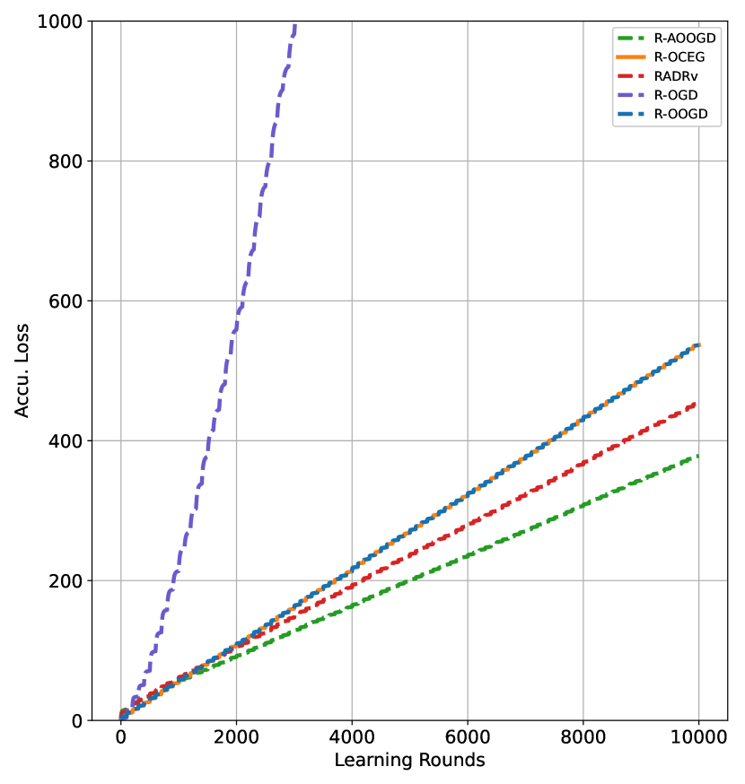
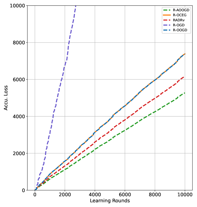
We test the online Fréchet mean on synthetic datasets generated as follows: In each iteration $t$, we randomly sample the point $A_{i,t}$ from a ball centered at a point $P_{t}$ with a radius of $c=1$. The choice of $P_{t}$ is in following two ways to simulate non-stationary environments. 1) $P_{t}$ remains fixed in between $S$ time steps. After every $S$ rounds, we re-select $P_{t}$ randomly within a bounded set of diameter $D=1$ to simulate abrupt changes in the environment. 2) $P_{t}$ shifts a small distance of $0.1$ between each time step, and is re-selected after $S$ round, to simulate a slowly evolving environment. For our experiment, we set $T=10000$, $n=100$, $d=20$, $D=1,\kappa=1$, and $L=\zeta(\kappa,D)$.

In addition, we compare our R-OOGD and R-AOOGD algorithms to other contenders in Riemannian online optimization. Specifically, we compare R-OOGD with the Riemannian online gradient descent (ROGD) algorithm [50] and the EG-type expert algorithm R-OCEG [29]. We also compare our meta-expert algorithm R-AOOGD with the meta-expert RADRv algorithm [29].

Result

We examine the performance in terms of cumulative loss and present the result in Fig 1. First, we can see that OGD suffers from a high cumulative loss throughout the horizon. Conversely, our methods, as well as R-OCEG and RADRv, demonstrate satisfactory performance in terms of dynamic regret in both situations. As meta-expert algorithms, our R-AOOGD slightly outperforms the RARDv. Our R-OOGD algorithm performs comparably to RARDv-exp, but with only half number of the gradient information required. These facts validate the effectiveness of our algorithms and demonstrate our advantage in situations where gradient computation is time-consuming.

(a) Stationary environment with abrupt changes

(b) Slowly evolving environment

Figure 1: Algorithm performance on hyperbolic Fréchet mean problems

6.2 Online Geodesic Regression

Geodesic Regression is a statistical model that generalizes the Euclidean least-square regression by modeling data as

$$y=\exp_{\hat{y}_{t}}(\epsilon),\quad\hat{y}_{t}=\exp_{p}(xV),$$

where $x\in\mathbb{R}$ is the feature, $y\in\mathcal{M}$ is the manifold-valued label, $V$ is a tangent vector at $P$, and $\epsilon$ is a Gaussian-distributed error. Geodesic Regression has many applications in medical imaging, object recognition, and linear system identification [52, 48, 26].

We can also consider an online form of geodesic regression, where the model is trained sequentially. For each data point ${x_{t},y_{t}}$, the online geodesic regression model minimizes the loss function

$$\mathbf{f}_{t}(p_{t},V_{t})=\frac{1}{2}d^{2}(\hat{y}_{t},y_{t})=\frac{1}{2}d^{2}(\exp_{p_{t}}(x_{t}V_{t}),y_{t}),$$

where $(p_{t},V_{t})\in T\mathcal{M}$ lies in the tangent bundle $T\mathcal{M}$ with the Sasaki metric [45],

$$\big{\langle}(p^{\prime}_{1},V^{\prime}_{1}),(p^{\prime}_{2},V^{\prime}_{2})\big{\rangle}=\langle p^{\prime}_{1},p^{\prime}_{2}\rangle_{\mathcal{M}}+\langle V^{\prime}_{1},V^{\prime}_{2}\rangle_{T_{P}\mathcal{M}}.$$

Experimental setting

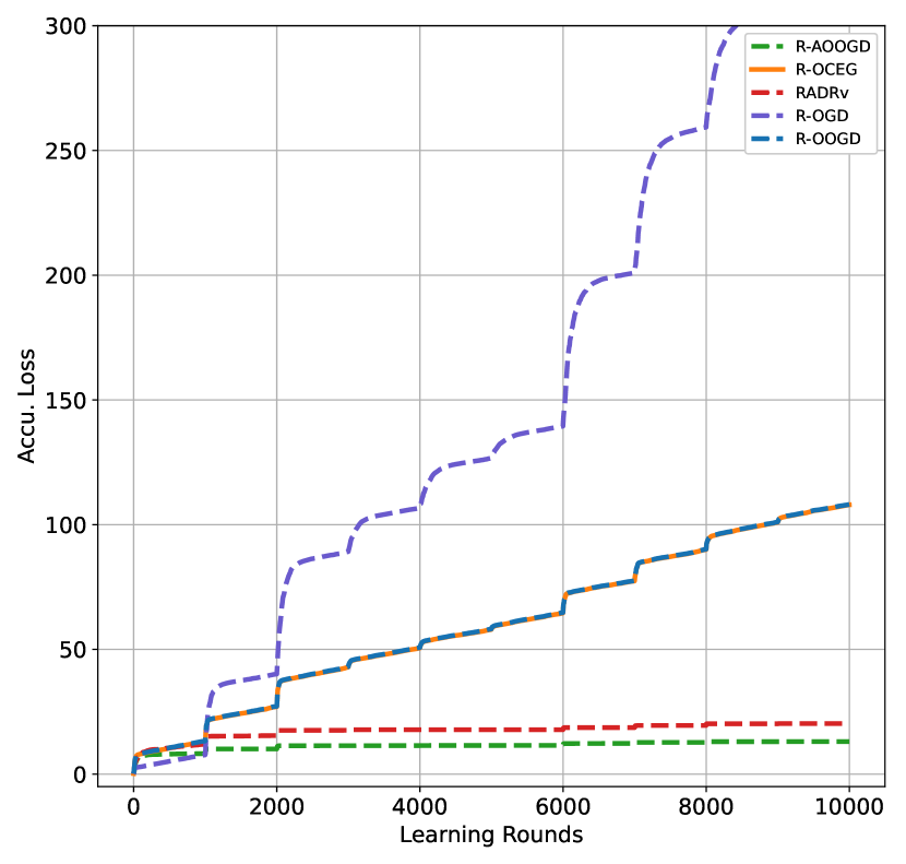
We now conduct our experiments on both synthetic and real-world dataset. The synthetic dataset is generated on a five-dimensional sphere $\mathbb{S}^{5}$. At each round, the feature $x_{t}$ is uniformly sampled from $[0,1]$, and the label $y_{t}$ is obtained as $y_{t}=\exp_{\hat{y}_{t}}(\epsilon_{t}),$ where $\hat{y}_{t}=\exp_{p_{t}}(x_{t}V_{t})$ and $\epsilon_{t}$ is a random tangent vector with norm chosen uniformly from $[0,0.1]$. Similar to the previous experiment, we fix $p_{t}$ and $V_{t}$ for $S$ rounds and randomly select new $p_{t}$ and $V_{t}$ from the half sphere after every $S$ rounds.

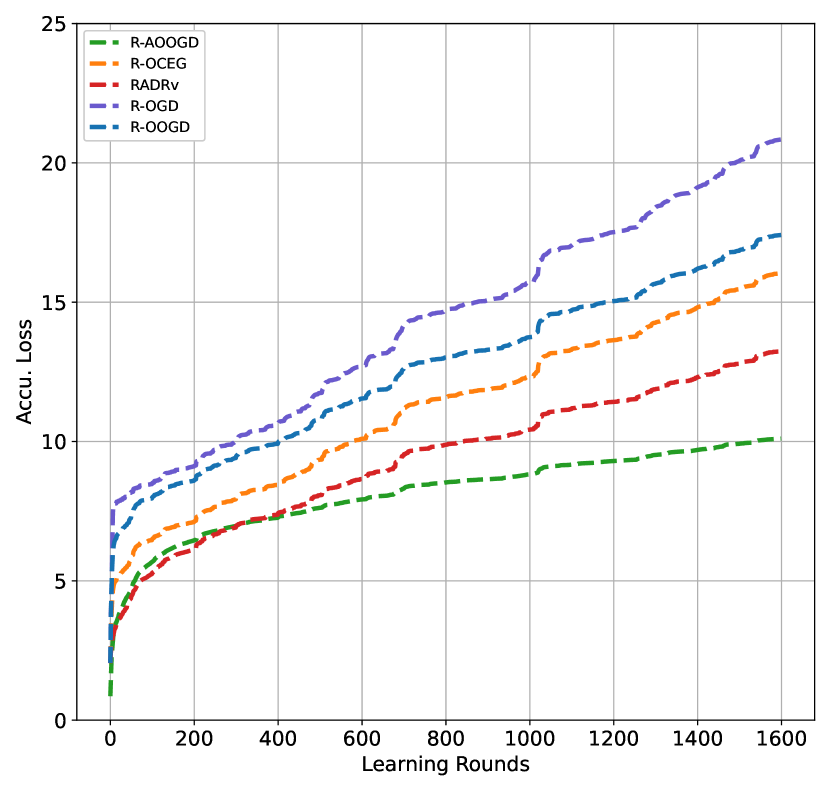
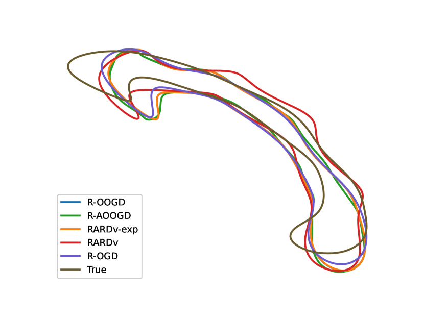
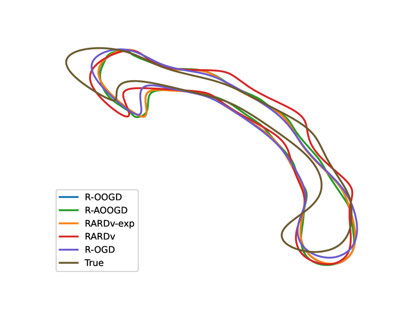
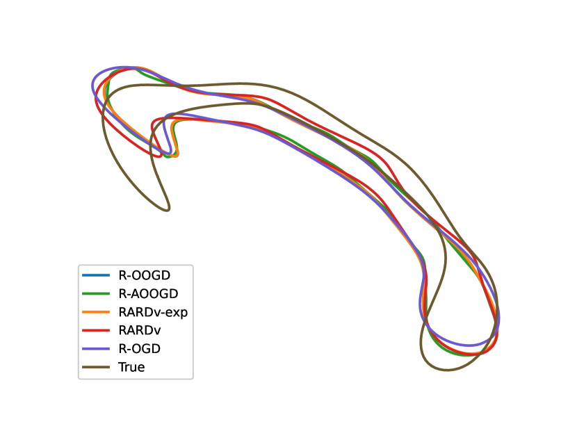
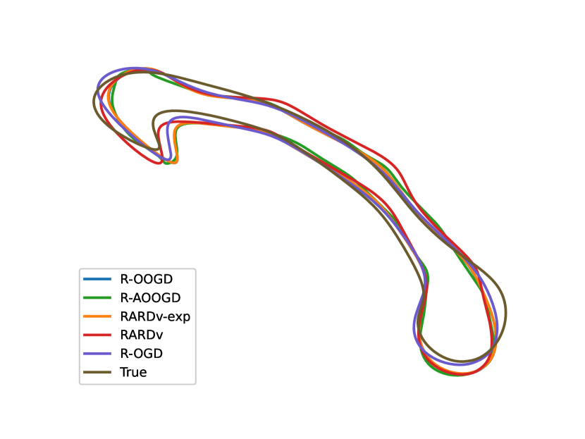
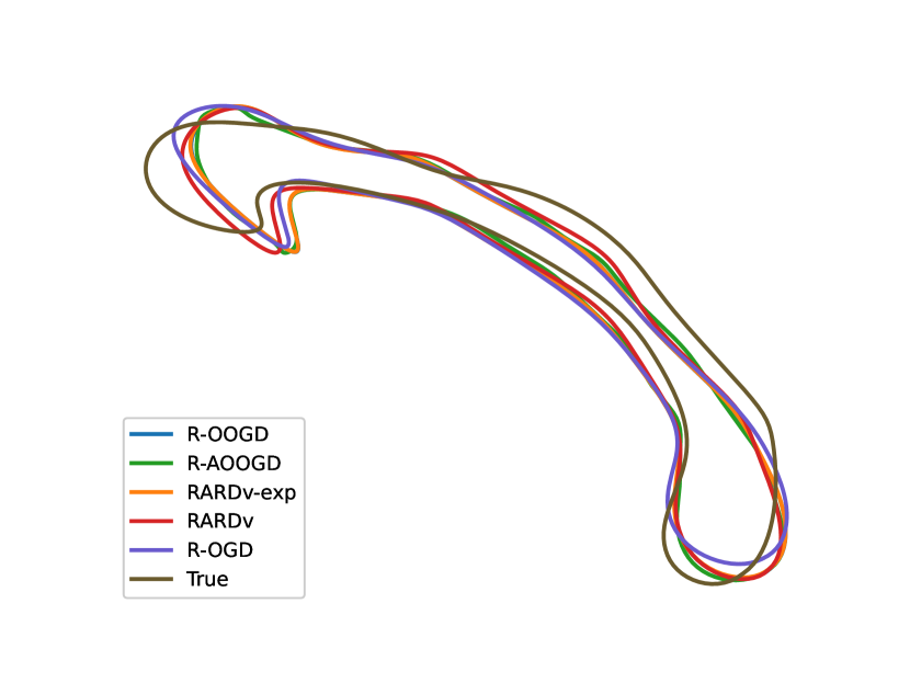
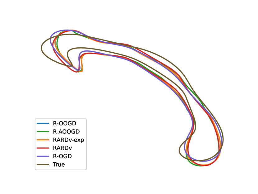
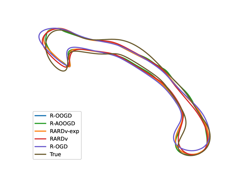
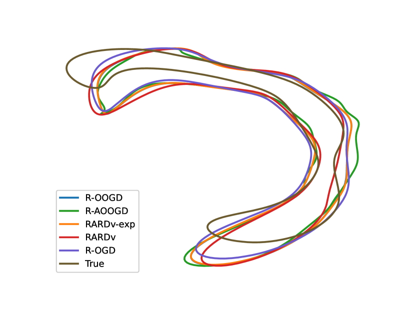
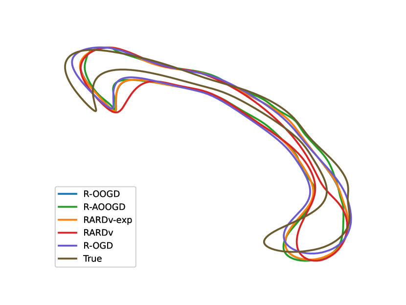
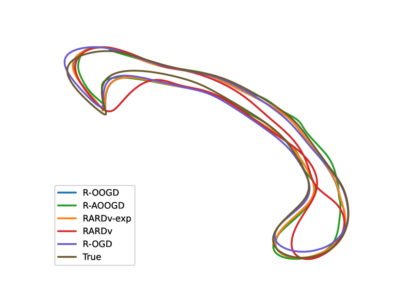
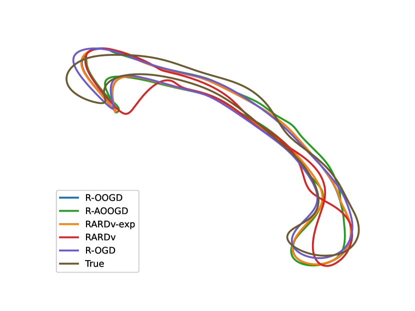
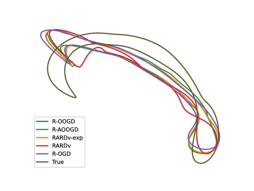
The real-world dataset used in this experiment is the corpus callosum dataset from the Alzheimer’s disease neuroimaging initiative, which was provided by [18] and can also be accessed online . The dataset includes information about 408 subjecst as well as shape of the subjects’ corpus callosum obtained from mid-sagittal slices of magnetic resonance images (MRI). The shape of an corpus callosum is described as a cloud point matrix $y_{t}\in\mathbb{R}^{50\times 2}$. During the experiment, we aimed to analyze the relationship between the age of the subjects and the shape of the corpus callosum by utilizing geodesic regression. To achieve this, we preprocessed the shape information into a Grassmann manifold $\mathcal{G}r(50,2)$ by computing the left-singular vectors of each $y_{t}$ as reported in a previous study by [26]. Then, we divided the $320$ data points into a training set and others to a testing set. Additionally, we duplicated training data points 5 times for efficient learning rounds.

Results

Figure 2 shows the accuracy and loss versus learning round for our algorithm. Additionally, we provide performance results on the test set of the corpus callosum shapes in Figure 3, which confirms the effectiveness of our R-OOGD algorithm and R-AOOGD algorithm in solving real-world problems. Our algorithm performs similarly or better than other state-of-the-art methods on both synthetic and real-world datasets, while requiring fewer gradient information. This finding aligns with our theoretical results.

It is noteworthy that we did not impose any special requirements on the boundedness of the training set in the real-world dataset. Therefore, our algorithm iterates over the entire Grassmann manifold with a diameter of $\frac{\sqrt{2}}{2}\pi>\frac{\pi}{2\sqrt{K}}=\frac{\pi}{2\sqrt{2}}$. This demonstrates the applicability of our algorithm when the diameter $D\geq\frac{\pi}{2\sqrt{K}}$.

(a) Synthetic data

(b) Real-world data

Figure 2: Algorithm performance on geodesic regression

(a) age=64

(b) age=66

(c) age=69

(d) age=70

(e) age=71

(f) age=73

(g) age=75

(h) age=77

(i) age=80

(j) age=83

(k) age=88

(l) age=90

Figure 3: Algorithm performance on testing set of corpus callosum shapes

6.3 Quadratic Geodesic Lodget Game

We now validate our theoretical finding in Riemannian zero-sum games. Consider the following toy-example RZS game

$$\min_{X\in\mathcal{S}_{d}^{++}}\max_{Y\in\mathcal{S}_{d}^{++}}c_{1}(\log\det(X))^{2}+c_{2}\log\det(X)\log\det(Y)-c_{1}(\log\det(Y))^{2},$$ (7)

where $X$ and $Y$ take values on the symmetric positive definite (SPD) matrix manifold

$$S^{++}_{d}:=\{X\in\mathbb{R}^{d\times d};X^{T}=X,X\succ 0\}$$

with affine-invariant metric

$$\langle U,V\rangle_{x}=tr(X^{-1}UX^{-1}V).$$

Since the logdet function is geodesic linear on $S^{++}_{d}$ [23], the quadratic game (7) is g-convex-concave with the g-strong convexity coefficient $c_{1}$. The NEs of the game (7) are $(X^{*},Y^{*})$ where $\det(X^{*})=\det(Y^{*})=1$.

Experimental setting

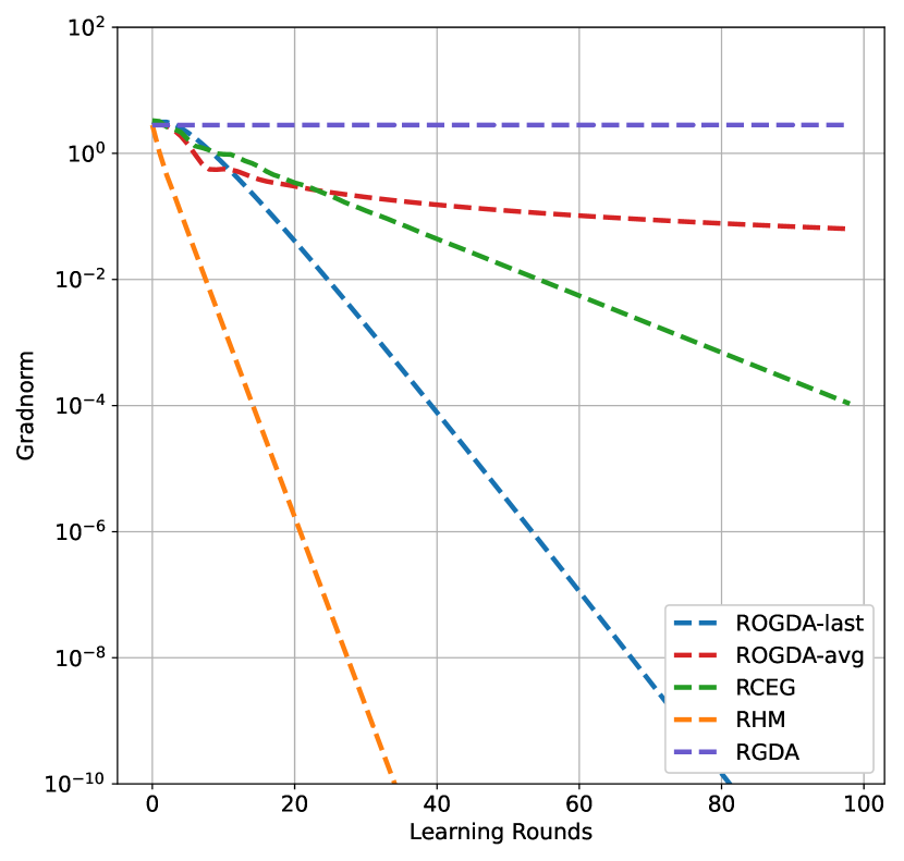
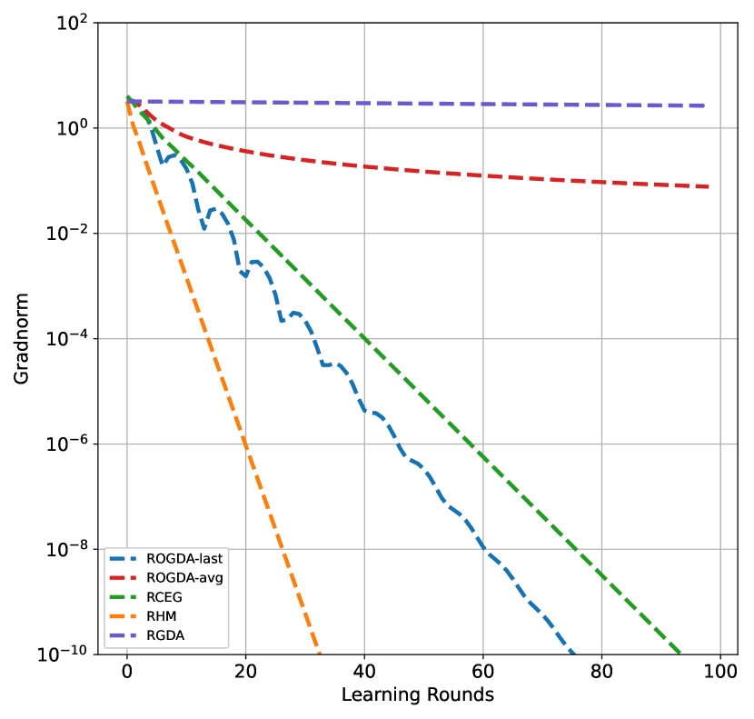
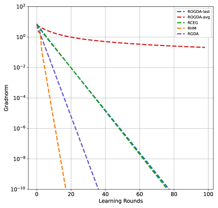
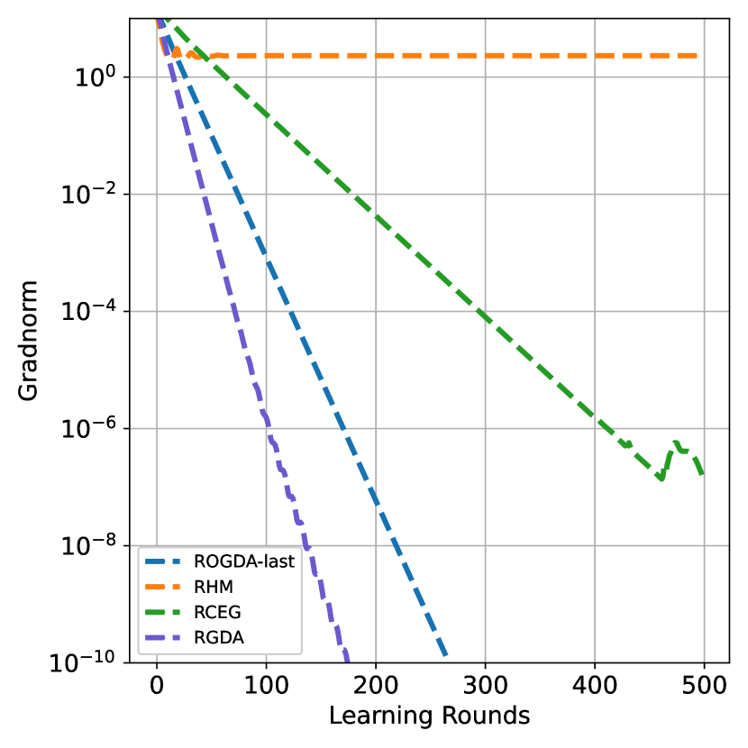
We test the R-OGDA in the case when $d=30$, $c_{2}=1$, and $c_{1}\in\{0,0.1,1\}$. We check the R-OGDA with the step size $\eta=0.5$ for $c_{1}\in\{0,0.1\}$ and $\eta=0.2$ for $c_{1}=1$. We also compare our algorithm with the second-order Riemannian Hamitonian method (RHM) [23], the Riemannian corrected extragradient method (RCEG) [55], and the Riemannian gradient descent ascent algorithm (R-GDA) [32] with the best-tuned step size.

(a) $c_{1}=0,c_{2}=1$

(b) $c_{1}=0.1,c_{2}=1$

(c) $c_{1}=1,c_{2}=1$

Figure 4: Quadratic geodesic lodget games

Results

We plot the norm of gradient $\|\nabla f(x_{t},y_{t})\|$ versus learning round $t$ in Figure 4. From the results, all the algorithm converge to the NE. Among them, the second-order algorithm RHM performs the best. For first-order algorithms, our R-OGDA algorithm shows good performance in both g-convex-concave and g-strongly convex-strongly concave scenarios. In comparison, R-GDA performs well in g-strongly convex-strongly concave scenarios but does not converge in linear cases (i.e., $c=0$). Similarly, RCEG shows slower convergence in linear scenarios and gradually improves with increasing g-strong convexity of the function, showing comparable convergence to our R-OGDA when $c=1$.

6.4 Robust Geometry-Aware PCA

Robust geometry-aware principal component analysis (PCA) [27] is a dimensional reduction tool for SPD matrices. Given a set of SPD matrices $\{A_{i}\}_{i=1}^{n}$, the geometry-aware PCA aims to find a geometry mean $A$ with the maximal data variance, which can be formulated as finding the NE in the following RZS game

$$\min_{A\in\mathcal{S}^{++}_{d}}\max_{X\in\mathbb{S}^{d}}X^{T}AX+\frac{\alpha}{n}\sum_{i}^{n}\|\log(A_{i}^{-\frac{1}{2}}AA_{i}^{-\frac{1}{2}})\|_{F},$$ (8)

where $\mathbb{S}^{d}$ is the $d$-dimensional unit sphere with the canonical metric $\langle U,V\rangle=U^{T}V$. The game (8) is g-strongly convex to $A$, but not g-concave to $X$. Hence, the game (8) is more challenging for our R-OGDA algorithm.

Experimental setting

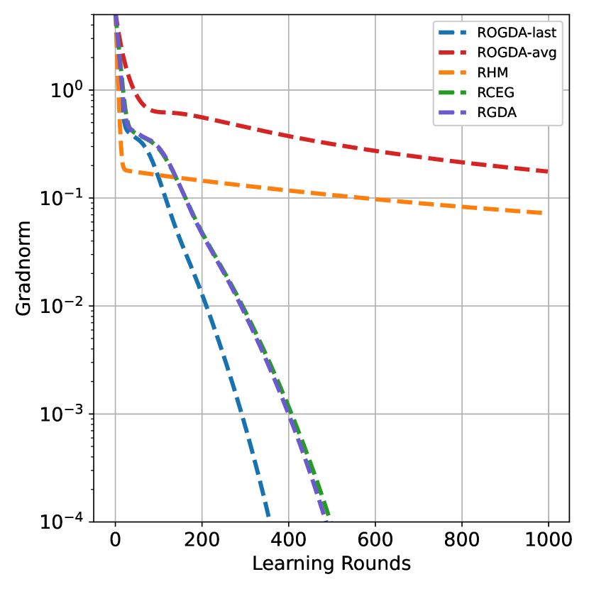
We run the experiment with a synthetic dataset $\{A_{i}\}_{i=1}^{n}$ and a real-world BCI dataset. The synthetic dataset is generated under conditions similar to those described in prior studies by [55] and [23], where the eigenvalues of $A_{i}$ are in $[0.2,4.5]$. The real-world dataset the BCI competition dataset IV [47]. The BCI competition dataset IV collected EEG signals from 59 channels electrodes of 5 subjects who executed left-hand, right-hand, foot and tongue movements. To preprocess the dataset, we follow the procedure outlined in [27], which involves selecting $200$ trials in the time interval from 0.5s to 2.5s, applying a band-pass filter to remove frequencies outside the 8–15Hz range and extracting covariant matrix into a $6\times 6$ matrix. For numerical stability, we divide the covariant matrix by $200$. For the synthetic dataset, we set the number of samples $n=40$, the dimension $d=50$, the regularization parameter $\alpha=1$, and the step size $\eta=0.07$. For the competition BCI dataset IV, we set $n=200$, $d=6$, $\alpha=1$ and $\eta=0.05$.

Results

As shown in Figure 5, on the synthetic datase, the R-OGDA has the fastest convergence rate. For the real world dataset, R-GDA performs the best and the R-OGDA outperforms the RHM and RCEG. The performance in the g-convex-nonconcave RZS games illustrates the potential value of the R-OGDA.

(a) synthetic dataset

(b) real-world dataset

Figure 5: Robust geometric-aware PCA

7 Conclusion

In this paper, we have investigated the dynamic regret of Riemannian online optimization. We proposed R-OOGD and established a dynamic regret bound of $\mathcal{O}(P_{T}\sqrt{1+V_{T}})$. Additionally, we introduced R-AOOGD, a meta-expertalgorithm that averages R-OOGD algorithms with different step sizes, which further improved the dynamic regret bound to $\mathcal{O}(\sqrt{(1+P_{T}+V_{T})(1+P_{T})})$. We also applied the ROGD algorithm to Riemannian zero-sum games and achieved convergence rates of $\mathcal{O}(\frac{1}{T})$ for average-iterate, $\mathcal{O}(\frac{1}{\sqrt{T}})$ for best-iterate, and $\mathcal{O}(e^{-\rho t})$ for last-iterate, for smooth g-convex-concave and g-strongly convex-strongly concave games. Our results demonstrate the impact of Riemannian geometry on algorithm performance, and all our regret bounds and convergence rates match the corresponding Euclidean results.

One possible future direction of our work is to consider Riemannian dynamic regret in the bandit feedback setting, where the learner only receives the function value $\mathbf{f}_{t}(x_{t})$ instead of the gradient $\nabla\mathbf{f}_{t}(x_{t})$. We plan to design Riemannian optimistic bandit algorithms by incorporating Riemannian optimization techniques into existing bandit optimization methods. This will make the resulting algorithms more effective in settings where obtaining gradients is difficult or even impossible, such as reinforcement learning on Riemannian manifolds.

Appendix A Definitions and Technical Lemmas

In the appendix, we introduce some prerequisite about Riemannian geometry for further analysis. In the rest of the appendix, we denote $\mathcal{X}(\mathcal{M})$ as the set of vector fields on the Riemannian manifold $\mathcal{M}$ and $C^{\infty}(\mathcal{M})$ as the class of infinitely differentiable functions on $\mathcal{M}$. A vector field $X$ is equivalent to an operator on $C^{\infty}(\mathcal{M})$ via the directional derivative $X(\mathbf{f}):=\lim_{t\to 0}\frac{1}{t}(\mathbf{f}(\gamma(t))-\mathbf{f}(t))$, where $\mathbf{f}\in C^{\infty}(\mathcal{M})$ and $\gamma$ is a curve such that $\gamma(0)=p$ and $\dot{\gamma}(0)=X(p)$.

First, we recall some definitions on Riemannian manifolds.

Definition 1 (35).

The gradient of a function $\mathbf{f}$ at the point $x$ is defined as the tangent vector $\nabla\mathbf{f}(x)\in T_{x}\mathcal{M}$ such that $\langle X(x),\nabla\mathbf{f}(x)\rangle=X(\mathbf{f})(x),\forall X\in\mathcal{X}(\mathcal{M})$.

Definition 2 (35).

The hessian of a function $f$ at the point $x$ is defined as the bilinear operator $\nabla^{2}\mathbf{f}(x):T_{x}\mathcal{M}\times T_{x}\mathcal{M}\to\mathbb{R}$ such that

$$\nabla^{2}\mathbf{f}(X(x),Y(x))(x)=\langle\nabla_{X}\nabla\mathbf{f}(x),Y(x)\rangle,\forall X,Y\in\mathcal{X}(\mathcal{M}).$$ (9)

Definition 3 (35).

A vector field $J$ along a geodesic $\gamma:[0,1]\to\mathcal{M}$ is a Jacobi field if it satisfies:

$$\langle\nabla_{\dot{\gamma}}\nabla_{\dot{\gamma}}J,W\rangle+R(\dot{\gamma},J,\dot{\gamma},W)=0,\quad\forall W\in\mathcal{X}(\mathcal{M}).$$

Then we recall some properties of the covariant derivative $\nabla_{X}Y$, the curvature tensor $R(X,Y,W,Z)$ and the Jacobi field.

Lemma 3 (13).

The covariant derivative $\nabla:\mathcal{X}(\mathcal{M})\times\mathcal{X}(\mathcal{M})\to\mathcal{X}(\mathcal{M})$ satisfies the following properties:

• $Z\langle X,Y\rangle=\langle\nabla_{Z}X,Y\rangle+\langle X,\nabla_{Z}Y\rangle,\quad\forall X,Y,Z\in\mathcal{X}(\mathcal{M})$;

• $\nabla_{X}Y-\nabla_{Y}X=[X,Y]$, where $[X,Y]=XY-YX$ is also a vector field on $\mathcal{M}$.

Lemma 4 (13).

If $\gamma:[0,1]\to\mathcal{M}$ is a curve on $M$ and $z\in T_{\gamma(0)}\mathcal{M}$. If we extend $z$ to a vector field $Z(t)\in T_{\gamma(t)}\mathcal{M}$ on $\gamma$ along the parallel transport $\Gamma_{\gamma(t)}$, then we have $\nabla_{\dot{\gamma}(t)}Z(t)=0$, $\forall t\in[0,1]$.

Lemma 5 (7).

Denote the curvature tensor

$$\langle\nabla_{X}\nabla_{Y}Z-\nabla_{Y}\nabla_{X}Z-\nabla_{[X,Y]}Z,W\rangle=R(X,Y,W,Z),$$

then the following statement hold.

• $R(X,Y,W,Z)$ is multilinear over $C^{\infty}(\mathcal{M})$ i.e.,

  $$R(f_{1}X,f_{2}Y,f_{3}W,f_{4}Z)=f_{1}f_{2}f_{3}f_{4}R(X,Y,W,Z),\quad\forall f_{1},f_{2},f_{3},f_{4}\in C^{\infty}(\mathcal{M}).$$

• The curvature tensor is determined by the its values on $2-$dimensional surfaces
  $\mathcal{K}(X,Y)=R(X,Y,X,Y)$, i.e.,

  $$6R(X,Y,W,Z) =\mathcal{K}(X+W,Y+Z)-\mathcal{K}(X,Y+Z)+\mathcal{K}(W,X+Z)$$

  $$\quad+\mathcal{K}(Y+W,X+Z)-\mathcal{K}(Y,X+Z)+\mathcal{K}(W,X+Z)$$

  $$\quad-\mathcal{K}(X+W,Y)+\mathcal{K}(X,Y)+\mathcal{K}(W,Y)$$

  $$\quad-\mathcal{K}(X+W,Z)+\mathcal{K}(X,Z)+\mathcal{K}(W,Z)$$

  $$\quad+\mathcal{K}(Y+W,X)+\mathcal{K}(Y,X)-\mathcal{K}(W,X)$$

  $$\quad+\mathcal{K}(Y+W,Z)-\mathcal{K}(Y,Z)-\mathcal{K}(W,Z).$$

Lemma 6 (Jacobi comparison theorem,35).

Suppose $\mathcal{M}$ is a Riemannian manifold and $\gamma:[0,b]\to\mathcal{M}$ is a geodesic with $\|\dot{\gamma}(0)\|=1$. $J$ is a Jacobi field along $\gamma$.

• If all sectional curvatures of $\mathcal{M}$ are upper bounded by a constant $K$, then denote

  $$\mathbf{S}(K,t)=\begin{cases}\frac{\sin(\sqrt{K}t)}{\sqrt{K}}&\quad K>0;\\ t&\quad K\leq 0.\end{cases}$$

  Then,

  $$\|J(\gamma(t))\|\geq\mathbf{S}(K,t)\|\nabla_{\dot{\gamma}}J(\gamma(0))\|$$

  for all $t\in[0,b_{1}]$, where $b_{1}=b$ if $K\leq 0$ and $b_{1}=\min(\frac{\pi}{\sqrt{K}},b)$ if $K\geq 0$.

• If all sectional curvatures of $\mathcal{M}$ are lower bounded by a constant $\kappa$, then denote

  $$\mathbf{s}(\kappa,t)=\begin{cases}\frac{\sinh(\sqrt{-\kappa}t)}{\sqrt{-\kappa}}&\quad\kappa<0;\\ t&\quad\kappa\geq 0.\end{cases}$$

  Then,

  $$\|J(\gamma(t))\|\leq\mathbf{s}(\kappa,t)\|\nabla_{\dot{\gamma}}J(\gamma(0))\|$$

  for all $t\in[0,b]$.

Furthermore, we consider two comparison inequalities, which served as the law of consine over Riemannian manifolds.

Lemma 7 (53).

Let $\mathcal{M}$ be a Riemannian manifold with all sectional curvatures lower bounded by $\kappa$. Denote

$$\zeta(\kappa,D)=\begin{cases}\frac{\sqrt{-\kappa}D}{\tanh(\sqrt{-\kappa}D)}&\kappa<0;\\ 1&\kappa\geq 0.\end{cases}$$

Then for a geodesic triangle $\triangle ABC$, we have

$$2\langle\exp^{-1}_{A}C,\exp^{-1}_{A}B\rangle\leq d^{2}(A,B)+\zeta(\kappa,d(A,B))d^{2}(A,C)-d^{2}(B,C).$$

Lemma 8 (5).

Let $\mathcal{M}$ be a Riemannian manifold with all sectional curvatures upper bounded by $K$. Denote

$$\sigma(K,D)=\begin{cases}\frac{\sqrt{K}D}{\tan(\sqrt{K}D)}&K>0;\\ 1&K\leq 0,\end{cases}\quad\text{and}\quad D(K)=\begin{cases}\infty&K\leq 0;\\ \frac{\pi}{2\sqrt{K}}&K>0.\end{cases}$$

If a geodesic triangle $\triangle ABC$ has diameter less than $D(K)$, then we have

$$2\langle\exp^{-1}_{A}C,\exp^{-1}_{A}B\rangle\geq d^{2}(A,B)+\sigma(K,d(A,B))d^{2}(A,C)-d^{2}(B,C).$$

In addtion, [3] demonstrate bi-Lipschitzness of the exponential map on positive curved space.

Lemma 9 (3).

Let $A,B,C$ be points on Riemannian manifold $\mathcal{M}$ with sectional curvatures upper bounded by $K\geq 0$. If $d(A,C)\leq\frac{\pi}{2\sqrt{K}}$, then

$$\|\exp^{-1}_{A}B-\exp^{-1}_{A}C\|\leq\sqrt{(1+2Kd^{2}(A,B))}d(B,C)\leq\frac{2}{\sqrt{\sigma(K,d(A,B))}}d(B,C).$$

Finally, we introduce a technique that bounds the metric distortion by parallel transport.

Lemma 10 (5).

Let $\mathcal{M}$ be a Riemannian manifold with sectional curvature lower bounded by $\kappa$ and upper bounded by $K$. If a geodesic triangle $\triangle ABC$ admits a diameter less than $D(K)$, then there exists a point $p$ in the edge $AC$ such that

$$\|\exp^{-1}_{A}B-\Gamma_{C}^{A}\exp^{-1}_{C}B\|=-\Gamma_{p}^{A}\big{(}\nabla^{2}(-\frac{1}{2}d^{2}(C,p))\big{)}\Gamma_{A}^{p}\exp^{-1}_{A}C,$$

where $\big{(}\nabla^{2}(-\frac{1}{2}d^{2}(C,p))\big{)}$ is the hessian of the function $-\frac{1}{2}d^{2}(C,\cdot)$ at point $p$.

We denote $H_{A,p}^{c}$ as the operator $-\Gamma_{p}^{A}\big{(}\nabla^{2}(-\frac{1}{2}d^{2}(C,p))\big{)}\Gamma_{A}^{p}$. From the hessian comparison theorem [35, 4], we know that all the eigenvalues of $H_{A,p}^{c}$ are in the range $[\sigma(K,d(C,p)),\zeta(\kappa,d(C,p))]$. Since

$$\max\big{\{}{\zeta(\kappa,d(C,p))-1,1-\sigma(K,d(C,p))}\big{\}}\leq\max({|\kappa|,|K|})d^{2}(C,p),$$

we have the following corollary.

Corollary 2.

Let $\mathcal{M}$ be a Riemannian manifold with sectional curvature lower bounded by $\kappa$ and upper bounded by $K$. If a geodesic triangle $\triangle ABC$ has diameter $D\leq D(K)$, then there exists a point $p$ lying in the edge $AC$ such that

• $\|\exp^{-1}_{A}B-\Gamma_{C}^{A}\exp^{-1}_{C}B\|\leq\zeta(\kappa,D)\|\exp^{-1}_{A}C\|$;

• $\|\exp^{-1}_{A}B-\Gamma_{C}^{A}\exp^{-1}_{C}B-\exp^{-1}_{A}C\|\leq d^{2}(C,p)\max\{|\kappa|,|K|\}\|\exp^{-1}_{A}C\|$.

Appendix B Proofs in Section 4

Proof of Theorem 1

To ease the notation, we define $v_{t}=\sup_{x\in\mathcal{K}}\|\mathbf{f}_{t}(x)-\mathbf{f}_{t-1}(x)\|^{2}$ and $\nabla_{t}=\nabla\mathbf{f}_{t}(x_{t})$. By the g-convexity of $\mathbf{f}_{t+1}$, we have

$$\mathbf{f}_{t+1}(x_{t+1})-\mathbf{f}_{t+1}(u_{t+1})\leq\langle\exp^{-1}_{x_{t+1}}u_{t+1},-\nabla_{t+1}\rangle.$$ (10)

Applying Lemma 8 in the geodesic triangle $\triangle x_{t+1}u_{t+1}x_{t}$ we have,

$$2\langle\exp^{-1}_{x_{t+1}}u_{t+1},\exp^{-1}_{x_{t+1}}x_{t}\geq d^{2}(x_{t+1},u_{t+1})-d^{2}(x_{t},u_{t+1})+\sigma_{0}d^{2}(x_{t+1},x_{t}).$$

Notice from Algorithm 1, we have $x_{t+1}=\exp_{x_{t}}(-2\eta\nabla_{t}+\eta\Gamma_{x_{t-1}}^{x_{t}}\nabla_{t-1})$. This give us

$$\exp^{-1}_{x_{t+1}}x_{t}=\eta(\Gamma_{x_{t}}^{x_{t+1}}(2\nabla_{t}-\Gamma_{x_{t-1}}^{x_{t}}\nabla_{t-1})).$$

Thus, we have

$$0\leq\langle\exp^{-1}_{x_{t+1}}u_{t+1}, \Gamma_{x_{t}}^{x_{t+1}}(2\nabla_{t}-\Gamma_{x_{t-1}}^{x_{t}}\nabla_{t-1})\rangle-$$

$$\qquad\frac{1}{2\eta}(d^{2}(x_{t+1},u_{t+1})-d^{2}(x_{t},u_{t+1}))-\frac{\sigma_{0}}{2\eta}d^{2}(x_{t+1},x_{t}).$$ (11)

Combining (10) and (B), we have

$$\mathbf{f}_{t+1}(x_{t+1})-\mathbf{f}_{t+1}(u_{t+1}) \leq\langle\exp^{-1}_{x_{t+1}}u_{t+1},-\nabla_{t+1}\rangle+\langle\exp^{-1}_{x_{t+1}}u_{t+1},\Gamma_{x_{t}}^{x_{t+1}}(2\nabla_{t}-\Gamma_{x_{t-1}}^{x_{t}}\nabla_{t-1})\rangle$$

$$\quad-\frac{1}{2\eta}(d^{2}(x_{t+1},u_{t+1})-d^{2}(x_{t},u_{t+1}))-\frac{\sigma_{0}}{2\eta}d^{2}(x_{t+1},x_{t})$$

$$=\langle\exp^{-1}_{x_{t+1}}u_{t+1},-\nabla_{t+1}+\Gamma_{x_{t}}^{x_{t+1}}\nabla_{t}\rangle$$

$$\quad-\langle\exp^{-1}_{x_{t+1}}u_{t+1},\Gamma_{x_{t}}^{x_{t+1}}(\nabla_{t}-\Gamma_{x_{t-1}}^{x_{t}}\nabla_{t-1})\rangle$$

$$\quad-\frac{1}{2\eta}(d^{2}(x_{t+1},u_{t+1})-d^{2}(x_{t},u_{t+1}))-\frac{\sigma_{0}}{2\eta}d^{2}(x_{t+1},x_{t}).$$ (12)

Considering the term $-\langle\exp^{-1}_{x_{t+1}}u_{t+1},\Gamma_{x_{t}}^{x_{t+1}}(\nabla_{t}-\Gamma_{x_{t-1}}^{x_{t}}\nabla_{t-1})\rangle-\frac{\sigma}{2\eta}d^{2}(x_{t},x_{t+1})$, we have

$$-\langle\exp^{-1}_{x_{t+1}}u_{t+1},\Gamma_{x_{t}}^{x_{t+1}}(\nabla_{t}-\Gamma_{x_{t-1}}^{x_{t}}\nabla_{t-1})\rangle-\frac{\sigma}{2\eta}d^{2}(x_{t},x_{t+1})$$

$$\leq\langle-\exp^{-1}_{x_{t+1}}u_{t+1}+\Gamma_{x_{t}}^{x_{t+1}}\exp^{-1}_{x_{t}}u_{t+1},\Gamma_{x_{t}}^{x_{t+1}}(\nabla_{t}-\Gamma_{x_{t-1}}^{x_{t}}\nabla_{t-1})\rangle$$

$$\quad+\langle-\exp^{-1}_{x_{t}}u_{t+1}+\exp^{-1}_{x_{t}}u_{t},\nabla_{t}-\Gamma_{x_{t-1}}^{x_{t}}\nabla_{t-1}\rangle$$

$$\quad-\langle\exp^{-1}_{x_{t}}u_{t},\nabla_{t}-\Gamma_{x_{t-1}}^{x_{t}}\nabla_{t-1}\rangle-\frac{\sigma_{0}}{2\eta}d^{2}(x_{t+1},x_{t}).$$ (13)

By Lemma 2, we have

$$\langle -\exp^{-1}_{x_{t+1}}u_{t+1}+\Gamma_{x_{t}}^{x_{t+1}}\exp^{-1}_{x_{t}}u_{t+1},\Gamma_{x_{t}}^{x_{t+1}}(\nabla_{t}-\Gamma_{x_{t-1}}^{x_{t}}\nabla_{t-1})\rangle$$

$$\leq\zeta_{0}d(x_{t+1},x_{t})\|\nabla_{t}-\Gamma_{x_{t-1}}^{x_{t}}\nabla_{t-1}\|$$

$$\leq\frac{\zeta_{0}^{2}}{\sigma_{0}}\eta\|\nabla_{t}-\Gamma_{x_{t-1}}^{x_{t}}\nabla_{t-1}\|^{2}+\frac{\sigma_{0}}{4\eta}d^{2}(x_{t},x_{t+1}).$$ (14)

The latter inequality is due to the Young’s inequality $\langle a,b\rangle\leq\frac{\alpha\|a\|^{2}}{2}+\frac{\|b\|^{2}}{2\alpha}$. Also, By Lemma 9, we have

$$\langle -\exp^{-1}_{x_{t}}u_{t+1}+\exp^{-1}_{x_{t}}u_{t},\nabla_{t}-\Gamma_{x_{t-1}}^{x_{t}}\nabla_{t-1}\rangle$$

$$\leq\frac{2}{\sqrt{\sigma}_{0}}d(u_{t},u_{t+1})\|\nabla_{t}-\Gamma_{x_{t-1}}^{x_{t}}\nabla_{t-1}\|$$

$$\leq\frac{1}{\sigma_{0}}\eta\|\nabla_{t}-\Gamma_{x_{t-1}}^{x_{t}}\nabla_{t-1}\|^{2}+\frac{d^{2}(u_{t+1},u_{t})}{\eta}$$

$$\leq\frac{1}{\sigma_{0}}\eta\|\nabla_{t}-\Gamma_{x_{t-1}}^{x_{t}}\nabla_{t-1}\|^{2}+\frac{d(u_{t+1},u_{t})D}{\eta}.$$ (15)

Since $\mathbf{f}_{t}$ is g-$L$-smooth, we have

$$\|\nabla_{t}-\Gamma_{x_{t-1}}^{x_{t}}\nabla_{t-1}\|^{2} \leq 2\|\nabla\mathbf{f}_{t}(x_{t})-\nabla\mathbf{f}_{t-1}(x_{t})\|^{2}+2\|\nabla\mathbf{f}_{t-1}(x_{t})-\Gamma_{x_{t-1}}^{x_{t}}\nabla_{t-1}\|^{2}$$

$$\leq 2v_{t}+2L^{2}d^{2}(x_{t},x_{t-1}).$$ (16)

Putting (B)-(B) together, we have

$$\mathbf{f}_{t+1}(x_{t+1})-\mathbf{f}_{t+1}(u_{t+1})\leq \langle\exp^{-1}_{x_{t+1}}u_{t+1},-\nabla_{t+1}+\Gamma_{x_{t}}^{x_{t+1}}\nabla_{t}\rangle-\langle\exp^{-1}_{x_{t}}u_{t},-\nabla_{t}+\Gamma_{x_{t-1}}^{x_{t}}\nabla_{t-1}\rangle$$

$$\quad+\frac{1}{2\eta}(d^{2}(x_{t},u_{t+1})-d^{2}(x_{t+1},u_{t+1}))$$

$$\quad+\frac{2(1+\zeta_{0}^{2})}{\sigma_{0}}\eta v_{t}+\frac{2L^{2}(1+\zeta_{0}^{2})}{\sigma_{0}}\eta d(x_{t},x_{t-1})$$

$$\quad+\frac{d(u_{t},u_{t+1})D}{\eta}-\frac{\sigma_{0}}{4\eta}d^{2}(x_{t},x_{t+1}).$$ (17)

Summing (B) from $t=0$ to $T-1$ together, we have

$${\sf{Reg}_{D}}(u_{1},u_{2},\dots,u_{T}) =\sum_{t=0}^{T-1}\mathbf{f}_{t+1}(x_{t+1})-\mathbf{f}_{t+1}(u_{t+1})$$

$$\leq\sum_{t=0}^{T-1}\langle\exp^{-1}_{x_{t+1}}u_{t+1},-\nabla_{t+1}+\Gamma_{x_{t}}^{x_{t+1}}\nabla_{t}\rangle$$

$$\quad-\sum_{t=0}^{T-1}\langle\exp^{-1}_{x_{t}}u_{t},-\nabla_{t}+\Gamma_{x_{t-1}}^{x_{t}}\nabla_{t-1}\rangle$$

$$\quad+\sum_{t=0}^{T-1}\frac{1}{2\eta}d^{2}(x_{t},u_{t+1})-\sum_{t=0}^{T-1}\frac{1}{2\eta}d^{2}(x_{t+1},u_{t+1})$$

$$\quad+\sum_{t=0}^{T-1}\frac{2L^{2}(1+\zeta_{0}^{2})}{\sigma_{0}}\eta d(x_{t},x_{t-1})-\sum_{t=0}^{T-1}\frac{\sigma_{0}}{4\eta}d^{2}(x_{t},x_{t+1}).$$

Rearranging the summation, we can obtain

$${\sf{Reg}_{D}}(u_{1},u_{2},\dots,u_{T}) \leq\frac{2(1+\zeta_{0}^{2})}{\sigma_{0}}\eta V_{T}+\frac{DP_{T}}{\eta}$$

$$\leq\sum_{t=1}^{T}\langle\exp^{-1}_{x_{t}}u_{t},-\nabla_{t}+\Gamma_{x_{t-1}}^{x_{t}}\nabla_{t-1}\rangle-\sum_{t=0}^{T-1}\langle\exp^{-1}_{x_{t}}u_{t},-\nabla_{t}+\Gamma_{x_{t-1}}^{x_{t}}\nabla_{t-1}\rangle$$

$$\quad+\sum_{t=0}^{T-1}\frac{1}{2\eta}d^{2}(x_{t},u_{t+1})-\sum_{t=1}^{T}\frac{1}{2\eta}d^{2}(x_{t},u_{t})$$

$$\quad+\sum_{t=0}^{T-1}\frac{4L^{2}\zeta_{0}^{2}}{\sigma_{0}}\eta d(x_{t},x_{t-1})-\sum_{t=1}^{T}\frac{\sigma_{0}}{4\eta}d^{2}(x_{t},x_{t-1})$$

$$\quad+\frac{4\zeta_{0}^{2}}{\sigma_{0}}\eta V_{T}+\frac{DP_{T}}{\eta}.$$

Since $\eta\leq\frac{\sigma_{0}}{4\zeta_{0}L}$, we have $\frac{4L^{2}\zeta_{0}^{2}\eta}{\sigma_{0}}\leq\frac{\sigma_{0}}{4\eta}$. Therefore, we have

$${\sf{Reg}_{D}}(u_{1},u_{2},\dots,u_{T}) =\sum_{t=0}^{T-1}\mathbf{f}_{t+1}(x_{t+1})-\mathbf{f}_{t+1}(u_{t+1})$$

$$\leq\langle\exp^{-1}_{x_{T}}u_{T},-\nabla_{T}+\Gamma_{x_{T-1}}^{x_{T}}\nabla_{T-1}\rangle-\langle\exp^{-1}_{x_{0}}u_{0},-\nabla_{0}+\Gamma_{x_{-1}}^{x_{0}}\nabla_{-1}\rangle$$

$$\quad+\frac{1}{2\eta}d^{2}(x_{0},u_{1})-\frac{1}{2\eta}d^{2}(x_{T},u_{T})$$

$$\quad+\frac{4L^{2}\zeta_{0}^{2}}{\sigma_{0}}\eta d(x_{0},x_{-1})-\frac{\sigma_{0}}{4\eta}d^{2}(x_{T},x_{T-1})$$

$$\quad+\frac{4\zeta_{0}^{2}}{\sigma_{0}}\eta V_{T}+\frac{2DP_{T}}{\eta}.$$

As $x_{-1}=x_{0}=x_{1}$, we can see that $\nabla_{0}=\nabla_{-1}$ and $d(x_{0},x_{-1})=0$. In this way, we can see that

$${\sf{Reg}_{D}}(u_{1},u_{2},\dots,u_{T}) =\sum_{t=0}^{T-1}\mathbf{f}_{t+1}(x_{t+1})-\mathbf{f}_{t+1}(u_{t+1})$$

$$\leq\langle\exp^{-1}_{x_{T}}u_{T},-\nabla_{T}+\Gamma_{x_{T-1}}^{x_{T}}\nabla_{T-1}\rangle+\frac{1}{2\eta}d^{2}(x_{0},u_{1})+\frac{4\zeta_{0}^{2}}{\sigma_{0}}\eta V_{T}+\frac{2DP_{T}}{\eta}$$

$$\leq 2DG+\frac{D^{2}}{2\eta}+\frac{4\zeta_{0}^{2}}{\sigma_{0}}\eta V_{T}+\frac{2DP_{T}}{\eta}$$

$$\leq\frac{D^{2}+2DP_{T}}{\eta}+\frac{4\zeta_{0}^{2}}{\sigma_{0}}\eta(V_{T}+G^{2}),$$

which completes our proof. $\blacksquare$

Proof of Theorem 2

We follow the idea to treat the dynamic regret by the meta-regret and expert-regret as in the work by [29]. For any $i\leq N$, it holds that

$$\sum_{t=1}^{T}\mathbf{f}_{t}(x_{t})-\mathbf{f}_{t}(u_{t})=\underbrace{\sum_{t=1}^{T}\mathbf{f}_{t}(x_{t})-\mathbf{f}_{t}(x_{i,t})}_{\mathtt{meta-regret}}+\underbrace{\sum_{t=1}^{T}\mathbf{f}_{t}(x_{t,i})-\mathbf{f}_{t}(u_{t})}_{\mathtt{expert-regret}}.$$

Based on Theorem 2 of [29], we obtain

$$\mathtt{meta}{\rm{-}}\mathtt{regret} =\sum_{t=1}^{T}\mathbf{f}_{t}(x_{t})-\mathbf{f}_{t}(x_{i,t})$$

$$\leq\frac{2+\ln N}{\beta}+3D_{0}^{2}\beta(V_{T}+G^{2})+$$

$$\quad+\sum_{t=2}^{T}\big{(}3\beta(D_{0}^{4}L^{2}+D_{0}^{2}G^{2}\zeta_{0}^{2})-\frac{1}{4\beta}\big{)}\|w_{t}-w_{t-1}\|_{1}^{2}$$

$$\leq\max\Big{(}2\sqrt{3D_{0}^{2}(V_{T}+G^{2})(2+\ln N)},2(2+\ln N)\sqrt{12(D_{0}^{4}L^{2}+D_{0}^{2}G^{2}\zeta_{0}^{2})}\Big{)}.$$

Moreover, according to the dynamic regret in Theorem 1, for any index $i$ with step size $\eta_{i}$, we have:

$$\mathtt{expert}{\rm{-}}\mathtt{regret} \leq\sum_{t=1}^{T}\mathbf{f}_{t}(x_{t,i})-\mathbf{f}_{t}(u_{t})$$

$$\leq\frac{D_{0}^{2}+2D_{0}P_{T}}{\eta_{i}}+\frac{4\zeta_{0}^{2}}{\sigma_{0}}\eta_{i}(V_{T}+G^{2}).$$

Our step size pool $\mathcal{H}=\Big{\{}\eta_{i}=2^{i-1}\sqrt{\frac{D_{0}^{2}}{16\zeta_{0}^{2}G^{2}T}}\Big{\}}$ ensures that

$$\begin{cases}\min_{\mathcal{H}}=\sqrt{\frac{D_{0}^{2}}{16\zeta_{0}^{2}G^{2}T}}\leq\sqrt{\frac{D_{0}^{2}+2D_{0}P_{T}}{4\zeta_{0}^{2}(G^{2}+V_{T})}},\\ \max_{\mathcal{H}}\geq\frac{\sigma_{0}}{\zeta_{0}L}.\end{cases}$$

So for the optimal step size $\eta^{*}=\min(\sqrt{\frac{D_{0}^{2}+P_{T}}{4\zeta_{0}^{2}(G^{2}+V_{T})}},\frac{\sigma_{0}}{\zeta_{0}L})$, there exists $i^{*}\leq N$ such that $\eta_{i^{*}}\leq\eta^{*}\leq 2\eta_{i^{*}}$. Taking $i=i^{*}$, we have

$$\mathtt{expert}{\rm{-}}\mathtt{regret} \leq\sum_{t=1}^{T}\mathbf{f}_{t}(x_{t,i})-\mathbf{f}_{t}(u_{t})$$

$$\leq\frac{D_{0}^{2}+2D_{0}P_{T}}{\eta_{i^{*}}}+\frac{4\zeta_{0}^{2}}{\sigma_{0}}\eta_{i^{*}}(V_{T}+G^{2})$$

$$\leq\frac{4\zeta_{0}^{2}}{\sigma_{0}}(V_{T}+G^{2})\sqrt{\frac{D_{0}^{2}+2D_{0}P_{T}}{4\zeta_{0}^{2}(G^{2}+V_{T})}}$$

$$\quad+(D_{0}^{2}+2D_{0}P_{T})(\sqrt{\frac{4\zeta_{0}^{2}(G^{2}+V_{T})}{D_{0}^{2}+2D_{0}P_{T}}}+\frac{4\zeta_{0}L}{\sigma_{0}})$$

$$\leq\frac{4\zeta_{0}}{\sqrt{\sigma_{0}}}\sqrt{(D_{0}^{2}+2D_{0}P_{T})((V_{T}+G^{2}))}+(D_{0}^{2}+2D_{0}P_{T})\frac{4\zeta_{0}L}{\sigma_{0}}.$$

Combining meta-regret and expert-regret together, we finally get

$$\sum_{t=1}^{T}\mathbf{f}_{t}(x_{t})-\mathbf{f}_{t}(u_{t}) \leq\max\Big{(}2\sqrt{3D_{0}^{2}(V_{T}+G^{2})(2+\ln N)},2(2+\ln N)\sqrt{12(D_{0}^{4}L^{2}+D_{0}^{2}G^{2}\zeta_{0}^{2})}\Big{)}$$

$$\quad+\frac{4\zeta_{0}}{\sqrt{\sigma_{0}}}\sqrt{(D_{0}^{2}+2D_{0}P_{T})((V_{T}+G^{2}))}+(D_{0}^{2}+2D_{0}P_{T})\frac{4\zeta_{0}L}{\sigma_{0}}$$

$$=\mathcal{O}(\sqrt{((V_{T}+1)\ln N)\ln N})+\frac{\zeta_{0}}{\sqrt{\sigma_{0}}}bo(\sqrt{(1+P_{T}+V_{T})(1+P_{T})})$$

$$=\frac{\zeta_{0}}{\sqrt{\sigma_{0}}}\mathcal{O}(\sqrt{(1+P_{T}+V_{T})(1+P_{T})}),$$

which completes our proof. $\blacksquare$

Appendix C Computing the Corrected R-OOGD

We first recall the corrected version of ROGD

$$\begin{cases}x_{t+1}=\exp_{x_{t}}(-2\eta\nabla_{t}+\exp^{-1}_{x_{t}}\hat{x}_{t})\\ \hat{x}_{t}=\exp_{x_{t-1}}(-\eta\nabla_{t-1}+\exp^{-1}_{x_{t-1}}\hat{x}_{t-1}).\end{cases}$$

To analyse the regret bound of the corrected version of R-OOGD, we follow (B) and get

$$0\leq\langle\exp^{-1}_{x_{t+1}}x,\Gamma_{x_{t+1}}^{x_{t}}(-2\eta\nabla_{t}+\exp^{-1}_{x_{t}}\hat{x}_{t})\rangle+\frac{1}{2\eta}(d^{2}(x_{t},x)-d^{2}(x_{t+1},x))-\frac{\sigma_{0}}{2\eta}d^{2}(x_{t+1},x_{t}).$$

Thus, by g-convexity we have,

$$\mathbf{f}_{t+1}(x_{t+1})-\mathbf{f}_{t+1}(x) \leq\langle\exp^{-1}_{x_{t+1}}x,-\nabla_{t+1}\rangle$$

$$\leq\langle\exp^{-1}_{x_{t+1}}x,-\nabla_{t+1}+\Gamma_{x_{t}}^{x_{t+1}}(-2\eta\nabla_{t}+\exp^{-1}_{x_{t}}\hat{x}_{t})\rangle$$

$$\quad+\frac{1}{2\eta}(d^{2}(x_{t},x)-d^{2}(x_{t+1},x))+\frac{\sigma_{0}}{2\eta}d^{2}(x_{t+1},x_{t})$$

$$=\langle\exp^{-1}_{x_{t+1}}x,\Gamma_{x_{t}}^{x_{t+1}}(\nabla_{t}-\Gamma_{x_{t-1}}^{x_{t}}\nabla_{t-1})\rangle$$

$$-\langle\exp^{-1}_{x_{t+1}}x,\nabla_{t+1}-\Gamma_{x_{t}}^{x_{t+1}}\nabla_{t}\rangle$$

$$\quad+\frac{1}{2\eta}(d^{2}(x_{t},x)-d^{2}(x_{t+1},x))-\frac{\sigma_{0}}{2\eta}d^{2}(x_{t+1},x_{t})$$

$$\quad+\langle\exp^{-1}_{x_{t+1}}x,-\Gamma_{x_{t}}^{x_{t+1}}\big{(}\Gamma_{x_{t-1}}^{x_{t}}\eta\nabla_{t-1}+\exp^{-1}_{x_{t}}\hat{x}_{t}\big{)}\rangle.$$ (18)

The expression (C) follows from the proof of Theorem 1 except the term

$$\langle\exp^{-1}_{x_{t+1}}x,-\Gamma_{x_{t}}^{x_{t+1}}\big{(}\Gamma_{x_{t-1}}^{x_{t}}\eta\nabla_{t-1}+\exp^{-1}_{x_{t}}\hat{x}_{t}\big{)}\rangle.$$

Applying Corollary 2 in the geodesic triangle $\triangle x_{t-1}x_{t}\hat{x}_{t}$, we have

$$\quad\|\exp^{-1}_{x_{t-1}}\hat{x}_{t}-\exp^{-1}_{x_{t-1}}x_{t}-\Gamma_{x_{t}}^{x_{t-1}}\exp^{-1}_{x_{t}}\hat{x}_{t}\|$$

$$=\|2\eta\nabla_{t-1}-\exp^{-1}_{x_{t-1}}\hat{x}_{t-1}-\eta\nabla_{t-1}+\exp^{-1}_{x_{t-1}}\hat{x}_{t-1}-\Gamma_{x_{t}}^{x_{t-1}}\exp^{-1}_{x_{t}}\hat{x}_{t}\|$$

$$\leq d^{2}(\hat{x}_{t},p)K_{m}\|\exp^{-1}_{x_{t-1}}x_{t}\|,$$

where $p$ lies in the geodesic $x_{t-1}x_{t}$. Since

$$d(\hat{x}_{t},p) \leq d(\hat{x}_{t},x_{t-1})+d(x_{t-1},x_{t})$$

$$\leq\|-2\eta\nabla_{t-1}+\eta\nabla_{t-2}-\eta\nabla_{t-2}+\exp^{-1}_{x_{t-1}}\hat{x}_{t-1}\|$$

$$\quad+\|-\eta\nabla_{t-1}+\eta\nabla_{t-2}-\eta\nabla_{t-2}+\exp^{-1}_{x_{t-1}}\hat{x}_{t-1}\|$$

$$\leq 5\eta G+2A_{t-1},$$

and

$$\|\exp^{-1}_{x_{t-1}}x_{t}\|\leq 3\eta G+A_{t-1},$$

we have:

$$A_{t}\leq K_{m}(5\eta G+2A_{t-1})^{2}(3\eta G+A_{t-1}),$$ (19)

indicating that the distortion in iteration $t-1$ evolves and accumulates in the distortion in iteration $t$. In the worst case scenario where $\eta G=0.1$ and $K_{m}=1$, the equality always holds. We observe that $A_{t}\to\infty$, which implies that the corrected ROGD fails to achieve sublinear static regret.

Appendix D Proof of Theorem 3

We first prove Lemma 1.

Proof of Lemma 1

We prove by induction on $z_{t}=(x_{t},y_{t})$. The base case $d(z_{0},z^{*})\leq D_{1}\leq 2D_{1}$ is straightforwardly hold. Then we assume that there exists a $K_{0}$ such that all $d(z_{t},z^{*})\leq 2D_{1}$ holds for all $t\leq K_{0}$. Then we carry out induction step on $K_{0}+1$. The distance $d(z_{K_{0}+1},z^{*})$ can be first bounded as

$$d(z_{K_{0}+1},z^{*})\leq d(z_{K_{0}},z^{*})+d(z_{K_{0}},z_{K_{0}+1})\leq 2D_{1}+3\eta G\leq 3D_{1}.$$

So, by setting $D_{0}=3D_{1}$, $\mathbf{f}_{t}(x)=\mathbf{f}(x,y_{t})$ and plugging in $u_{1}=u_{2}=\dots=u_{n}=x^{*}$ in the analysis of Theorem 1, the R-OOGD for player-$\mathtt{X}$ holds for all $t\leq K_{0}$

$$\langle\exp^{-1}_{x_{t+1}}x^{*},-\nabla_{x}\mathbf{f}(x_{t+1},y_{t+1})\rangle$$

$$\leq\langle\exp^{-1}_{x_{t+1}}x^{*},\big{(}\nabla_{x}\mathbf{f}(x_{t+1},y_{t+1})-\Gamma_{x_{t}}^{x_{t+1}}\nabla_{y}\mathbf{f}(x_{t},y_{t})-\big{(}\nabla_{x}\mathbf{f}(x_{t},y_{t})\big{)}-\Gamma_{x_{t-1}}^{x_{t}}\mathbf{f}(x_{t-1},y_{t-1})\big{)}\rangle$$

$$\quad+\frac{1}{2\eta}(d^{2}(x_{t},x^{*})-d^{2}(x_{t+1},x^{*}))-\frac{\sigma_{1}}{2\eta}d^{2}(x_{t},x_{t+1})$$

$$\leq\langle\exp^{-1}_{x_{t+1}}x^{*},\nabla_{x}\mathbf{f}(x_{t+1},y_{t+1})-\Gamma_{x_{t}}^{x_{t+1}}\mathbf{f}(x_{t},y_{t})\rangle$$

$$\quad-\langle\exp^{-1}_{x_{t}}x^{*},\nabla_{x}\mathbf{f}(x_{t},y_{t})-\Gamma_{x_{t-1}}^{x_{t}}\mathbf{f}(x_{t-1},y_{t-1})\rangle+\frac{1}{2\eta}(d^{2}(x_{t},x^{*})-d^{2}(x_{t+1},x^{*}))$$

$$\quad-\frac{\sigma_{1}}{2\eta}d^{2}(x_{t},x_{t+1})+\zeta_{1}\|\nabla_{x}\mathbf{f}(x_{t},y_{t})-\Gamma_{x_{t-1}}^{x_{t}}\mathbf{f}(x_{t-1},y_{t-1})\|d(x_{t},x_{t+1}).$$ (20)

Similarly, the player-$\mathtt{Y}$ holds for all $t\leq K_{0}$

$$\langle\exp^{-1}_{y_{t+1}}y^{*},\nabla_{y}\mathbf{f}(x_{t+1},y_{t+1})\rangle$$

$$\leq\langle\exp^{-1}_{y_{t+1}}y^{*},\nabla_{y}\mathbf{f}(x_{t+1},y_{t+1})-\Gamma_{y_{t}}^{y_{t+1}}\nabla_{y}\mathbf{f}(x_{t},y_{t})\rangle$$

$$\quad-\langle\exp^{-1}_{y_{t}}y^{*},\nabla_{y}\mathbf{f}(x_{t},y_{t})-\Gamma_{y_{t-1}}^{y_{t}}\nabla_{y}\mathbf{f}(x_{t-1},y_{t-1})\rangle+\frac{1}{2\eta}(d^{2}(y_{t},y^{*})-d^{2}(y_{t+1},y^{*}))$$

$$\quad-\frac{\sigma_{1}}{2\eta}d^{2}(y_{t},y_{t+1})+\zeta_{1}\|\nabla_{y}\mathbf{f}(x_{t},y_{t})-\Gamma_{y_{t-1}}^{y_{t}}\nabla_{y}\mathbf{f}(x_{t-1},y_{t-1})\|d(y_{t},y_{t+1}).$$ (21)

Adding (D) and (D) together, for all $t\leq K_{0}+1$, we have

$$0 \leq\langle\exp^{-1}_{z_{t+1}}z^{*},-\mathbf{F}(z_{t+1})\rangle$$

$$\leq\langle\exp^{-1}_{z_{t+1}}z^{*},-\mathbf{F}(z_{t+1})+\Gamma_{z_{t}}^{z_{t+1}}\mathbf{F}(z_{t})\rangle-\langle\exp^{-1}_{z_{t}}z^{*},-\mathbf{F}(z_{t})+\Gamma_{z_{t-1}}^{z_{t}}\mathbf{F}(z_{t-1})\rangle$$

$$\quad+\frac{1}{2\eta}(d^{2}(x_{t},x^{*})+d^{2}(y_{t},y^{*}))-\frac{1}{2\eta}(d^{2}(x_{t+1},x^{*})+d^{2}(y_{t+1},y^{*}))$$

$$\quad+\zeta_{1}\|\nabla_{y}\mathbf{f}(x_{t},y_{t})-\Gamma_{y_{t-1}}^{y_{t}}\nabla_{y}\mathbf{f}(x_{t-1},y_{t-1})\|d(y_{t},y_{t+1})$$

$$\quad+\zeta_{1}\|\nabla_{x}\mathbf{f}(x_{t},y_{t})-\Gamma_{x_{t-1}}^{x_{t}}\mathbf{f}(x_{t-1},y_{t-1})\|d(x_{t},x_{t+1})$$

$$\quad-\frac{\sigma_{1}}{2\eta}d^{2}(x_{t},x_{t+1})-\frac{\sigma_{1}}{2\eta}d^{2}(y_{t},y_{t+1}).$$ (22)

Taking Young’s inequality with

$$\begin{cases}a=(d(x_{t},x_{t+1}),d(y_{t},y_{t+1}))\\ b=(\|\nabla_{x}\mathbf{f}(x_{t},y_{t})-\Gamma_{x_{t-1}}^{x_{t}}\mathbf{f}(x_{t-1},y_{t-1})\|,\|\nabla_{y}\mathbf{f}(x_{t},y_{t})-\Gamma_{y_{t-1}}^{y_{t}}\nabla_{y}\mathbf{f}(x_{t-1},y_{t-1})\|),\\ \alpha=L,\end{cases}$$

we have

$$a\cdot b \leq\frac{L}{2}(d^{2}(x_{t},x_{t+1})+d^{2}(y_{t},y_{t+1}))$$

$$\quad+\frac{1}{2L}(\|\nabla_{x}\mathbf{f}(x_{t},y_{t})-\Gamma_{x_{t-1}}^{x_{t}}\mathbf{f}(x_{t-1},y_{t-1})\|^{2}+\|\nabla_{y}\mathbf{f}(x_{t},y_{t})-\Gamma_{y_{t-1}}^{y_{t}}\nabla_{y}\mathbf{f}(x_{t-1},y_{t-1})\|^{2}).$$

$$\leq\frac{L}{2}d^{2}(z_{t},z_{t+1})+\frac{1}{2L}L^{2}d^{2}(z_{t-1},z_{t})=\frac{L}{2}(d^{2}(z_{t},z_{t+1})+d^{2}(z_{t-1},z_{t})).$$ (23)

Plugging (D) into (D) yields

$$0 \leq\langle\exp^{-1}_{z_{t+1}}z^{*},-\mathbf{F}(z_{t+1})\rangle$$

$$\leq\langle\exp^{-1}_{z_{t+1}}z^{*},-\mathbf{F}(z_{t+1})+\Gamma_{z_{t}}^{z_{t+1}}\mathbf{F}(z_{t})\rangle-\langle\exp^{-1}_{z_{t}}z^{*},-\mathbf{F}(z_{t})+\Gamma_{z_{t-1}}^{z_{t}}\mathbf{F}(z_{t-1})\rangle$$

$$\quad+\frac{1}{2\eta}(d^{2}(z_{t},z^{*})-d^{2}(z_{t+1},z^{*}))+\frac{\zeta_{1}L}{2}(d^{2}(z_{t},z_{t+1})+d^{2}(z_{t-1},z_{t}))-\frac{\sigma_{1}}{2\eta}d^{2}(z_{t},z_{t+1}).$$ (24)

Since $\eta\leq\frac{\zeta_{1}}{2\sigma_{1}L}$, we have $-\frac{\sigma_{1}}{2\eta}+\frac{\zeta_{1}L}{2}\leq-\frac{\zeta_{1}L}{2}$, which gives us

$$0 \leq\langle\exp^{-1}_{z_{t+1}}z^{*},-\mathbf{F}(z_{t+1})\rangle$$

$$\leq\langle\exp^{-1}_{z_{t+1}}z^{*},-\mathbf{F}(z_{t+1})+\Gamma_{z_{t}}^{z_{t+1}}\mathbf{F}(z_{t})\rangle-\langle\exp^{-1}_{z_{t}}z^{*},-\mathbf{F}(z_{t})+\Gamma_{z_{t-1}}^{z_{t}}\mathbf{F}(z_{t-1})\rangle$$

$$\quad+\frac{1}{2\eta}(d^{2}(z_{t},z^{*})-d^{2}(z_{t+1},z^{*}))+\frac{\zeta_{1}L}{2}(-d^{2}(z_{t},z_{t+1})+d^{2}(z_{t-1},z_{t})).$$ (25)

By summing (D) from $t=0$ to $K_{0}$, we observe that

$$0 \leq\sum_{t=0}^{K_{0}}\langle\exp^{-1}_{z_{t+1}}z^{*},-\mathbf{F}(z_{t+1})\rangle$$

$$\leq\langle\exp^{-1}_{z_{K_{0}+1}}z^{*},-\mathbf{F}(z_{K_{0}+1})+\Gamma_{z_{K_{0}}}^{z_{K_{0}+1}}\mathbf{F}(z_{K_{0}})\rangle-\langle\exp^{-1}_{z_{0}}z^{*},-\mathbf{F}(z_{-1})+\Gamma_{z_{-1}}^{z_{0}}\mathbf{F}(z_{-1})\rangle$$

$$\quad+\frac{1}{2\eta}d^{2}(z_{0},z^{*})-\frac{1}{2\eta}d^{2}(z_{K_{0}+1},z^{*})-\frac{\zeta_{1}L}{2}d^{2}(z_{K_{0}},z_{K_{0}+1})+\frac{\zeta_{1}L}{2}d^{2}(z_{0},z_{-1}).$$

Furthermore, based on the fact that $z_{0}=z_{-1}$, we can express that

$$0 \leq\sum_{t=0}^{K_{0}}\langle\exp^{-1}_{z_{t+1}}z^{*},-\mathbf{F}(z_{t+1})\rangle$$

$$\leq\langle\exp^{-1}_{z_{K_{0}+1}}z^{*},-\mathbf{F}(z_{K_{0}+1})+\Gamma_{z_{K_{0}}}^{z_{K_{0}+1}}\mathbf{F}(z_{K_{0}})\rangle$$

$$+\frac{1}{2\eta}d^{2}(z_{0},z^{*})-\frac{1}{2\eta}d^{2}(z_{K_{0}+1},z^{*})-\frac{\zeta_{1}L}{2}d^{2}(z_{K_{0}},z_{K_{0}+1}).$$

Using g-$L$-smoothness again, we have

$$0 \leq\sum_{t=0}^{K_{0}}\langle\exp^{-1}_{z_{t+1}}z^{*},-\mathbf{F}(z_{t+1})\rangle$$

$$\leq Ld(z_{K_{0}+1},z^{*})d(z_{K_{0}+1},z_{K_{0}})+\frac{1}{2\eta}d^{2}(z_{0},z^{*})-\frac{1}{2\eta}d^{2}(z_{K_{0}+1},z^{*})-\frac{\zeta_{1}L}{2}d^{2}(z_{K_{0}},z_{K_{0}+1})$$

$$\leq\frac{L}{2}(d^{2}(z_{K_{0}+1},z^{*})+d^{2}(z_{K_{0}+1},z_{K_{0}}))+\frac{1}{2\eta}d^{2}(z_{0},z^{*})$$

$$\quad-\frac{1}{2\eta}d^{2}(z_{K_{0}+1},z^{*})-\frac{\zeta_{1}L}{2}d^{2}(z_{K_{0}},z_{K_{0}+1})$$

$$\leq\frac{L}{2}d^{2}(z_{K_{0}+1},z^{*})+\frac{1}{2\eta}d^{2}(z_{0},z^{*})-\frac{1}{2\eta}d^{2}(z_{K_{0}+1},z^{*}).$$

The last inequality is due to $\zeta_{1}\geq 1$, and the inequality gives us

$$d^{2}(z_{K_{0}+1},z^{*})\leq\frac{1}{1-\eta L}d^{2}(z_{0},z^{*})\leq\frac{1}{1-\frac{\sigma_{1}}{2\zeta_{1}}}d^{2}(z_{0},z^{*})\leq 2d^{2}(z_{0},z^{*})=2D_{1}^{2}.$$

Thus, $d^{2}(z_{t},z^{*})\leq 2D_{1}^{2}$ holds for $t=K_{0}+1$, By mathematical induction, the claim $d^{2}(z_{t},z^{*})\leq 2D_{1}$ holds for all $t\geq 0$, which completes our proof. $\blacksquare$

Now we shift our focus on proof of Theorem 3.

Proof of Theorem 3

By the g-convexity-concavity, for any $(x,y)\in\mathcal{M}\times\mathcal{N}$, there holds

$$\begin{cases}\sum_{t=1}^{T}\mathbf{f}(x_{t},y)-\sum_{t=1}^{T}\mathbf{f}(x_{t},y_{t})\leq\sum_{t=1}^{T}\langle\nabla_{y}\mathbf{f}(x_{t},y_{t}),\exp^{-1}_{y_{t}}y\rangle\\ \sum_{t=1}^{T}\mathbf{f}(x_{t},y_{t})-\sum_{t=1}^{T}\mathbf{f}(x,y_{t})\leq\sum_{t=1}^{T}\langle-\nabla_{x}\mathbf{f}(x_{t},y_{t}),\exp^{-1}_{x_{t}}x\rangle.\end{cases}$$

In this way, there holds

$$\sum_{t=1}^{T}\mathbf{f}(x_{t},y)-\sum_{t=1}^{T}\mathbf{f}(x,y_{t}) \leq\sum_{t=1}^{T}\langle\nabla_{y}\mathbf{f}(x_{t},y_{t}),\exp^{-1}_{y_{t}}y\rangle+\sum_{t=1}^{T}\langle-\nabla_{x}\mathbf{f}(x_{t},y_{t}),\exp^{-1}_{x_{t}}x\rangle$$

$$=\sum_{t=1}^{T}\langle-\mathbf{F}(z_{t}),\exp^{-1}_{z_{t}}z\rangle.$$

From the proof of Lemma 1, we can obtain

$$\sum_{t=1}^{T}\mathbf{f}(x_{t},y)-\sum_{t=1}^{T}\mathbf{f}(x,y_{t}) \leq\sum_{t=1}^{T}\langle-\mathbf{F}(z_{t}),\exp^{-1}_{z_{t}}z\rangle$$

$$\leq\langle\exp^{-1}_{z_{T}}z,-\mathbf{F}(z_{T})+\Gamma_{z_{T-1}}^{z_{T}}\mathbf{F}(z_{T-1})\rangle+\frac{1}{2\eta}d^{2}(z_{0},z^{*})$$

$$\quad-\frac{1}{2\eta}d^{2}(z_{K_{0}+1},z^{*})-\frac{\zeta_{1}L}{2}d^{2}(z_{K_{0}},z_{K_{0}+1})$$

$$\leq 2D_{1}G+\frac{1}{\eta}D_{1}^{2}.$$

To complete the proof, it remains to show that

$$\mathbf{f}(\bar{x}_{T},y)-\mathbf{f}(x,\bar{y}_{T})\leq\frac{1}{T}\sum_{t=1}^{T}\mathbf{f}(x_{t},y)-\frac{1}{T}\sum_{t=1}^{T}\mathbf{f}(x,y_{t}),$$

which can be proved by induction

$$\mathbf{f}(\bar{x}_{T},y) =\mathbf{f}(\exp_{\bar{x}_{t}}(\frac{1}{T}\exp^{-1}_{\bar{x}_{T-1}}x_{T}),y)$$

$$\leq\frac{1}{T}\mathbf{f}(x_{T},y)+\frac{T-1}{T}\mathbf{f}(\bar{x}_{T-1},y)$$

$$\leq\frac{1}{T}\mathbf{f}(x_{T},y)+\frac{T-1}{T}\frac{1}{T-1}\mathbf{f}(x_{T-1},y)+\frac{T-1}{T}\frac{T-2}{T-1}\mathbf{f}(\bar{x}_{T-2},y)$$

$$\leq\frac{1}{T}\mathbf{f}(x_{T},y)+\frac{1}{T}\mathbf{f}(x_{T-1},y)+\cdots+\frac{1}{T}\mathbf{f}(x_{2},y)+\frac{1}{T}\mathbf{f}(\bar{x}_{1},y)$$

$$=\frac{1}{T}\sum_{t=1}^{T}\mathbf{f}(x_{t},y),$$

and

$$\mathbf{f}(x,\bar{y}_{T}) =\mathbf{f}(x,\exp_{\bar{y}_{t}}(\frac{1}{T}\exp^{-1}_{\bar{y}_{T-1}}y_{T}))$$

$$\geq\frac{1}{T}\mathbf{f}(x,y_{T})+\frac{T-1}{T}\mathbf{f}(x,\bar{y}_{T-1})$$

$$\geq\frac{1}{T}\mathbf{f}(x,y_{T})+\frac{1}{T}\mathbf{f}(x,y_{T-1})+\cdots+\frac{1}{T}\mathbf{f}(x,y_{2})+\frac{1}{T}\mathbf{f}(x,\bar{y}_{1})$$

$$=\frac{1}{T}\sum_{t=1}^{T}\mathbf{f}(x,y_{t}).$$

Then Theorem 3 has been established. $\hfill\blacksquare$

Appendix E Proof of Lemma 2

We first propose some lemmas that are useful in proving Lemma 2.

Lemma 11 (A variant of Gauss-Bonnet theorem, 35, 16).

Suppose $M$ is a manifold with sectional curvature in $[\kappa,K]$ and $\Xi(s,t):[0,1]\times[0.1]\to\mathcal{M}$ is a rectangle map. $\Gamma_{\gamma}$ is the parallel transport around the boundary curve $\gamma$ that $\gamma=\Xi(t,0)\cup\Xi(1,s)\cup\Xi(t,1)\cup\Xi(0,s)$. Denote vector fields $S(\Xi(s,t))=\Xi_{*}\frac{\partial}{\partial s}(s,t)$, $T(\Xi(s,t))=\Xi_{*}\frac{\partial}{\partial t}(s,t)$ and $K_{m}=\max(|\kappa|,|K|)$. Then we have

$$\|\Gamma_{\gamma}z-z\|\leq 12K_{m}\|z\|\int_{0}^{1}\int_{0}^{1}\|T\|\|S\|dsdt,\forall z\in T_{\Xi(0,0)}\mathcal{M}.$$

Proof.

We first extend $z$ to a vector field $Z(s_{0},t_{0})=Z(\Xi(s_{0},t_{0}))$ by first parallel transporting $z$ along the curve $\Xi(0,t),(0\leq t\leq t_{0})$ and then parallel transporting along the curve $\Xi(s,t_{0}),(0\leq s\leq s_{0})$. It shows that

$$\begin{cases}\nabla_{S}Z(s,t)=0\\ \nabla_{T}Z(0,t)=0\end{cases}\forall(s,t)\in[0,1]\times[0,1].$$

For an arbitrary vector $w\in T_{\Xi(0,0)}\mathcal{M}$, we also extend it to $W(s_{0},t_{0})$ by first parallel transporting along the curve $\Xi(s,0),(0\leq s\leq 1)$, then along the curve $\Xi(1,t),(0\leq t\leq t_{0})$, and along the curve $\Xi(s,t_{0}),(1\geq s\geq s_{0})$. We can also have

$$\begin{cases}\nabla_{S}W(s,t)=0\\ \nabla_{T}W(1,t)=0\end{cases}\forall(s,t)\in[0,1]\times[0,1].$$

We denote two curves that $\xi_{1}=\Xi(s,0),(0\leq s\leq 1)$ and $\xi_{2}=\Xi(s,0)\cup\Xi(1,t),(0\leq s,t\leq 1)$. By the above notation, we find

$$\langle\Gamma_{\gamma}z-z,w\rangle =\langle\Gamma_{\gamma}z,w\rangle-\langle z,w\rangle$$

$$=\langle\Gamma_{\xi_{2}}\Gamma_{\gamma}z,\Gamma_{\xi_{2}}w\rangle-\langle\Gamma_{\xi_{1}}z,\Gamma_{\xi_{2}}w\rangle.$$

From the way we extend $Z$ and $W$, we know that $\Gamma_{\xi_{2}}\Gamma_{\gamma}z=Z(1,1)$, $\Gamma_{\xi_{2}}w=W(1,1)$, $\Gamma_{\xi_{1}}z=Z(1,0)$, and $\Gamma_{\xi_{2}}w=W(1,0)$, thus we have

$$\langle\Gamma_{\gamma}z-z,w\rangle =\langle Z(1,1),W(1,1)\rangle-\langle Z(1,0)-W(1,0)\rangle$$

$$=\int_{0}^{1}\frac{\partial}{\partial t}\langle Z(1,t),W(1,t)\rangle dt$$

$$=\int_{0}^{1}T\langle Z(1,t),W(1,t)\rangle dt$$

$$=\int_{0}^{1}\langle\nabla_{T}Z(1,t),W(1,t)\rangle+\langle Z(1,t),\nabla_{T}W(1,t)\rangle dt.$$

Due to the fact that $\nabla_{T}W(1,t)=0$, we have

$$\langle\Gamma_{\gamma}z-z,w\rangle =\int_{0}^{1}\langle\nabla_{T}Z(1,t),W(1,t)\rangle dt$$

$$=\int_{0}^{1}\Big{(}\langle\nabla_{T}Z(0,t),W(0,t)\rangle+\int_{0}^{1}\partial_{s}\langle\nabla_{T}Z(s,t),W(s,t)\rangle ds\big{)}dt$$

$$=\int_{0}^{1}\int_{0}^{1}\langle\frac{\partial}{\partial s}\langle\nabla_{T}Z(s,t),W(s,t)\rangle dsdt$$

$$=\int_{0}^{1}\int_{0}^{1}S\langle\nabla_{T}Z(s,t),W(s,t)\rangle dsdt$$

$$=\int_{0}^{1}\int_{0}^{1}\langle\nabla_{S}\nabla_{T}Z(s,t),W(s,t)\rangle+\langle\nabla_{T}Z(s,t),\nabla_{S}W(s,t)\rangle dsdt$$

$$=\int_{0}^{1}\int_{0}^{1}\langle\nabla_{S}\nabla_{T}Z(s,t),W(s,t)\rangle dsdt.$$

The last equality is from the fact that $\nabla_{S}W(s,t)=0$. Since the curvature has the form

$$R(S,T,Z,W)=\langle\nabla_{S}\nabla_{T}Z(s,t),W(s,t)\rangle+\langle\nabla_{T}\nabla_{S}Z(s,t),W(s,t)\rangle+\langle\nabla_{[S,T]}Z(s,t),W(s,t)\rangle$$

and we have $\nabla_{S}Z(s,t)=0$, $[S,T]=0$, it holds that

$$\langle\Gamma_{\gamma}z-z,w\rangle =\int_{0}^{1}\int_{0}^{1}R(S,T,Z,W)dsdt$$

$$=\int_{0}^{1}\int_{0}^{1}R(\frac{S}{\|S\|},\frac{T}{\|T\|},\frac{Z}{\|Z\|},\frac{W}{\|W\|})\|S\|\|T\|\|W\|\|Z\|dsdt.$$

By Lemma 5 and $R(X,Y,X,Y)\leq K_{m}\|X\|^{2}\|Y\|^{2}$, we have

$$R(\frac{S}{\|S\|},\frac{T}{\|T\|},\frac{Z}{\|Z\|},\frac{W}{\|W\|})\leq 12K_{m}.$$

Hence,

$$\langle\Gamma_{\gamma}z-z,w\rangle \leq 12K_{m}\int_{0}^{1}\int_{0}^{1}\|S\|\|T\|\|W\|\|Z\|dsdt$$

$$=12K_{m}\|z\|\|w\|\int_{0}^{1}\int_{0}^{1}\|S\|\|T\|dsdt,$$

which completes our proof since $w$ is arbitary. ∎

Lemma 12.

Suppose $M$ is a manifold with sectional curvature in $[\kappa,K]$ and $\gamma:[0,b]\to\mathcal{M}$ is a geodesic with $\|\dot{\gamma}(0)\|=1$ ($b\leq\frac{\pi}{\sqrt{K}}$ if $K>0$). If $J$ is a Jacobi field along $\gamma$ with $\|J(\gamma(0))\|=\alpha_{1}$ and $\|J(\gamma(b))\|=\alpha_{2}$, then we have

$$\|J(\gamma(t))\|\leq\frac{\mathbf{s}(\kappa,b)}{\mathbf{S}(K,b)}(\alpha_{1}+\alpha_{2}).$$

Proof.

We split $J(\gamma(t))=J_{1}(\gamma(t))+J_{2}(\gamma(t))$, where $J_{1}$ is a Jacobi field such that $J_{1}(\gamma(0))=0$ and $J_{1}(\gamma(b))=J(\gamma(b))$, and where $J_{2}$ is a Jacobi field such that $J_{2}(\gamma(b))=0$ and $J_{2}(\gamma(0))=J(\gamma(0))$. Applying the Jacobi comparison theorem (Lemma 6), we have

$$\begin{cases}\mathbf{S}(K,b)\|\nabla_{\dot{\gamma}}J_{1}(0)\|\leq\|J_{1}(\gamma(b))\|=\alpha_{2}\\ \mathbf{S}(K,b)\|\nabla_{\dot{\gamma}}J_{2}(b)\|\leq\|J_{2}(\gamma(0))\|=\alpha_{1},\end{cases}$$ (26)

and

$$\begin{cases}\|J_{1}(\gamma(t))\|\leq\mathbf{s}(\kappa,t)\|\nabla_{\dot{\gamma}}J_{1}(0)\|\leq\mathbf{s}(\kappa,b)\|\nabla_{\dot{\gamma}}J_{1}(0)\|\\ \|J_{2}(\gamma(t))\|\leq\mathbf{s}(\kappa,(b-t))\|\nabla_{\dot{\gamma}}J_{2}(b)\|\leq\mathbf{s}(\kappa,b)\|\nabla_{\dot{\gamma}}J_{2}(b)\|.\end{cases}$$ (27)

Combining (26) and (27) we have

$$\begin{cases}\|J_{1}(\gamma(t))\|\leq\frac{\mathbf{s}(\kappa,b)}{\mathbf{S}(K,b)}\alpha_{1}\\ \|J_{2}(\gamma(t))\|\leq\frac{\mathbf{s}(\kappa,b)}{\mathbf{S}(K,b)}\alpha_{2},\end{cases}$$

which gives us

$$\|J(\gamma(t))\|\leq\|J_{1}(\gamma(t))\|+\|J_{2}(\gamma(t))\|\leq\frac{\mathbf{s}(\kappa,b)}{\mathbf{S}(K,b)}(\alpha_{1}+\alpha_{2}).$$

This completes the proof. ∎

Lemma 13.

Denote $K_{m}=\max(|\kappa|,|K|)$. If $0\leq b\leq\frac{1}{\sqrt{K_{m}}}$, then we have $\frac{\mathbf{s}(\kappa,b)}{\mathbf{S}(K,b)}\leq 3.$

Proof.

It suffice to proof the lemma in the case $K\geq 0$ and $\kappa\leq 0$. We first consider the case where $K>0$ and $\kappa<0$, where

$$\frac{\mathbf{s}(\kappa,b)}{\mathbf{S}(K,b)}=\frac{\sqrt{K}\sinh(\sqrt{-k}b)}{\sqrt{-\kappa}\sin(\sqrt{K}b)}.$$ (28)

We show that $\cosh(ax)\leq(1+a^{2}x^{2})$ for $0\leq x\leq\frac{1}{a}$. Let

$$f(x)=\cosh(ax)-1-a^{2}x^{2}.$$

We have

$$\begin{cases}f(0)=0\\ f^{\prime}(x)=a\sinh(ax)-2a^{2}x,f^{\prime}(0)=0\\ f^{\prime\prime}(x)=a^{2}(\cosh(ax)-2).\end{cases}$$

Since $\cosh(ax)-2\leq 0$ for $0\leq x\leq\frac{1}{a}$, we have $f(x)\leq 0$ for $0\leq x\leq\frac{1}{a}$.

Then we show that $\frac{\sinh(ax)}{\sin(cx)}\leq\frac{a}{c}+\frac{a(a^{2}+c^{2})x^{2}}{c}$ for $0\leq x\leq\frac{1}{a}$. By defining

$$g(x)=\sinh(ax)-(\frac{a}{c}+\frac{a(a^{2}+c^{2})x^{2}}{c})\sin(cx),$$

we have

$$\begin{cases}g(0)=0\\ g^{\prime}(x)=a\cosh(ax)-(a+ax^{2}(a^{2}+c^{2}))\cos cx-(\frac{2a(a^{2}+c^{2})x}{c}))\sin cx\\ \end{cases}$$

As $0\leq x\leq\frac{1}{a}$, we have

$$g^{\prime}(x) \leq a(1+a^{2}x^{2})-(a+ax^{2}(a^{2}+c^{2}))\cos cx-(\frac{2a(a^{2}+c^{2})x}{c}))\sin cx$$

$$\leq a(1+a^{2}x^{2})(1-\cos cx)-2acx\sin cx$$

$$\leq a(1+a^{2}x^{2})(1-\cos^{2}cx)-2a\sin^{2}cx$$

$$=a(1+a^{2}x^{2})\sin^{2}cx-2a\sin^{2}cx$$

$$\leq a(-1+a^{2}x^{2})\sin^{2}cx$$

$$\leq 0$$

And thus, we have

$$\sinh(ax)-(\frac{a}{c}+\frac{a(a^{2}+c^{2})x^{2}}{c})\sin(cx)\leq 0,\quad 0\leq x\leq\frac{1}{a}$$

which is equivalent to

$$\frac{\sinh(ax)}{\sin(cx)}\leq\frac{a}{c}+\frac{a(a^{2}+c^{2})x^{2}}{c},\quad 0\leq x\leq\frac{1}{a}$$ (29)

Putting (28) into (29) with $a=\sqrt{-\kappa}$ and $c=\sqrt{K}$, we have, for $0\leq b\leq\frac{1}{\sqrt{K_{m}}}$

$$\frac{\mathbf{s}(\kappa,b)}{\mathbf{S}(K,b)} =\frac{\sqrt{K}\sinh(\sqrt{-k}b)}{\sqrt{-\kappa}\sin(\sqrt{K}b)}$$

$$\leq 1+(\kappa+K)b^{2}.$$

$$\leq 1+2K_{m}\frac{1}{K_{m}}$$

$$\leq 3,$$

which completes the proof for the where case $K>0$ and $\kappa<0$. Since $\frac{\mathbf{s}(\kappa,b)}{\mathbf{S}(K,b)}$ is continuous on $K$ and $\kappa$, we have proved the case with $K=0$ or $\kappa=0$ by continuity. ∎

Lemma 14.

In Algorithm 4, if $\eta\leq\frac{1}{8L}$, it satisfies

$$\frac{1}{2}\leq\frac{\|\mathbf{F}(z_{t+1})\|}{\|\mathbf{F}(z_{t})\|}\leq\frac{3}{2}.$$ (30)

The proof is as same as that the prior work by [14], so we omit the proof.

Then we begin our proof of Lemma 2.

Proof of Lemma 2

We first estimate the length $d(z_{t-1},z_{t})$ by,

$$d(z_{t-1},z_{t}) =\|2\eta\mathbf{F}(z_{t-1})-\Gamma_{z_{t-2}}^{z_{t-1}}\eta(\mathbf{F}(z_{t-2}))\|$$

$$\leq\eta\|\mathbf{F}(z_{t-1})\|+\eta\|\mathbf{F}(z_{t-1})-\Gamma_{z_{t-2}}^{z_{t-1}}(\mathbf{F}(z_{t-2}))\|$$

$$\leq\eta\|\mathbf{F}(z_{t-1})\|+\eta Ld(z_{t-1},z_{t-2})$$

$$=\eta\|\mathbf{F}(z_{t-1})\|+\eta L\|2\mathbf{F}(z_{t-2})-\Gamma_{z_{t-3}}^{z_{t-2}}\mathbf{F}(z_{t-3})\|$$

$$\leq\eta\|\mathbf{F}(z_{t-1})\|+\eta L(\|2\mathbf{F}(z_{t-2})\|+\|\mathbf{F}(z_{t-3})\|).$$

By Lemma 14, we have $\|\mathbf{F}(z_{t-2})\|\leq 2\|\mathbf{F}(z_{t-1})\|$ and $\|\mathbf{F}(z_{t-3})\|\leq 4\|\mathbf{F}(z_{t-1})\|$. So, we have

$$d(z_{t-1},z_{t})\leq(1+8L\eta)\eta\|\mathbf{F}(z_{t-1})\|.$$ (31)

Similarly, $d(\hat{z}_{t+1},z_{t})$ and $d(\hat{z}_{t},z_{t-1})$ can be bounded by

$$d(\hat{z}_{t+1},z_{t}) =\|\eta\mathbf{F}(z_{t})-\Gamma_{z_{t-1}}^{z_{t}}\mathbf{F}(z_{t-1})\|$$

$$\leq L\eta d(z_{t},z_{t-1})$$

$$\leq L\eta^{2}\|2\eta\mathbf{F}(z_{t-1})-\Gamma_{z_{t-2}}^{z_{t-1}}\eta(\mathbf{F}(z_{t-2}))\|$$

$$\leq L\eta^{2}(2\|\mathbf{F}(z_{t-1})\|+\|\mathbf{F}(z_{t-2})\|)$$

$$\leq 4L\eta^{2}\|\mathbf{F}(z_{t-1})\|,$$

and

$$d(\hat{z}_{t},z_{t-1}) =\eta\|\mathbf{F}(z_{t-1})-\Gamma_{z_{t-2}}^{z_{t-1}}(\mathbf{F}(z_{t-2}))\|$$

$$\leq L\eta^{2}\|2\mathbf{F}(z_{t-2})-\Gamma_{z_{t-3}}^{z_{t-2}}(\mathbf{F}(z_{t-3}))\|$$

$$\leq 8L\eta^{2}\|\mathbf{F}(z_{t-1})\|.$$

Consequently, the $l_{t}:=d(z_{t-1},z_{t})+d(\hat{z}_{t+1},z_{t})+d(\hat{z}_{t},z_{t-1})$ has the bound

$$l_{t} \leq(1+8L\eta)\eta\|\mathbf{F}(z_{t-1})\|+4L\eta^{2}\|\mathbf{F}(z_{t-1})\|+8L\eta^{2}\|\mathbf{F}(z_{t-1})\|$$

$$\leq(1+20L\eta)\eta\|\mathbf{F}(z_{t-1})\|.$$

Since $\eta\leq\frac{1}{20L}$, we have

$$l_{t}\leq 2\eta\|\mathbf{F}(z_{t-1})\|.$$ (32)

Now we examine (i). Applying Lemma 2 in the geodesic triangle $\triangle z_{t-1}\hat{z}_{t+1}z_{t}$ yields

$$\exp^{-1}_{z_{t-1}}\hat{z}_{t+1}=H_{z_{t-1},p_{1}}^{\hat{z}_{t+1}}\exp^{-1}_{z_{t-1}}z_{t}+\Gamma_{z_{t}}^{z_{t-1}}\exp^{-1}_{z_{t}}\hat{z}_{t+1},$$ (33)

where $p_{1}$ lies in the geodesic between $z_{t-1}$ and $z_{t}$. Applying Lemma 2 in the geodesic triangle $\triangle z_{t-1}\hat{z}_{t+1}\hat{z}_{t}$ yields

$$\exp^{-1}_{z_{t-1}}\hat{z}_{t+1}=H_{z_{t-1},p_{2}}^{\hat{z}_{t+1}}\exp^{-1}_{z_{t-1}}\hat{z}_{t}+\Gamma_{\hat{z}_{t}}^{z_{t-1}}\exp^{-1}_{\hat{z}_{t}}\hat{z}_{t+1}.$$ (34)

where $p_{2}$ lies in the geodesic between $z_{t-1}$ and $\hat{z}_{t}$.

Combing (33) and (34), we have

$$H_{z_{t-1},p_{2}}^{\hat{z}_{t+1}} (-\eta\mathbf{F}(z_{t-1})+\eta\Gamma_{z_{t-2}}^{z_{t-1}}\mathbf{F}(z_{t-2}))-\Gamma_{\hat{z}_{t}}^{z_{t-1}}\Gamma_{\hat{z}_{t+1}}^{\hat{z}_{t}}G_{t+1}$$

$$=H_{z_{t-1},p_{1}}^{\hat{z}_{t+1}}(-2\eta\mathbf{F}(z_{t-1})+\eta\Gamma_{z_{t-2}}^{z_{t-1}}\mathbf{F}(z_{t-2}))+\Gamma_{z_{t}}^{z_{t-1}}(-\eta\mathbf{F}(z_{t})+\Gamma_{z_{t-1}}^{z_{t}}\eta\mathbf{F}(z_{t-1})).$$ (35)

Rearranging (E), we have

$$\Gamma_{\hat{z}_{t}}^{z_{t-1}}\Gamma_{\hat{z}_{t+1}}^{\hat{z}_{t}}G_{t+1}-\Gamma_{z_{t}}^{z_{t-1}}(\eta\mathbf{F}(z_{t})) =(H_{z_{t-1},p_{2}}^{\hat{z}_{t+1}}-Id)(-\eta\mathbf{F}(z_{t-1})+\eta\Gamma_{z_{t-2}}^{z_{t-1}}\mathbf{F}(z_{t-2}))$$

$$\quad-(H_{z_{t-1},p_{1}}^{\hat{z}_{t+1}}-Id)(-2\eta\mathbf{F}(z_{t-1})+\eta\Gamma_{z_{t-2}}^{z_{t-1}}\mathbf{F}(z_{t-2})).$$

By Corollary 2, we have

$$\|\Gamma_{\hat{z}_{t}}^{z_{t-1}}\Gamma_{\hat{z}_{t+1}}^{\hat{z}_{t}}G_{t+1}-\eta\Gamma_{z_{t}}^{z_{t-1}}\mathbf{F}(z_{t})\| \leq K_{m}d^{2}(\hat{z}_{t+1},p_{1})d(z_{t-1},\hat{z}_{t})+K_{m}d^{2}(\hat{z}_{t+1},p_{2})d(z_{t-1},z_{t}).$$

Since $p_{1}$ lies in the geodesic between $z_{t-1}$ and $z_{t}$, we have $d(\hat{z}_{t+1},p_{1})\leq d(\hat{z}_{t+1},z_{t})+d(\hat{z}_{t},z_{t-1})\leq l_{t}$. Also, we have $d(\hat{z}_{t+1},p_{2})\leq l_{t}$. Then, we have

$$\|\Gamma_{\hat{z}_{t}}^{z_{t-1}}\Gamma_{\hat{z}_{t+1}}^{\hat{z}_{t}}G_{t+1}-\eta\Gamma_{z_{t}}^{z_{t-1}}\mathbf{F}(z_{t})\| \leq K_{m}l_{t}^{2}(d(z_{t-1},\hat{z}_{t})+d(z_{t-1},z_{t}))$$

$$\leq K_{m}l_{t}^{3}=K_{m}8\eta^{3}\|\mathbf{F}(z_{t-1})\|^{3}.$$

Then,

$$\|G_{t+1}\|^{2}-\|\eta\mathbf{F}(z_{t})\|^{2} =\|\Gamma_{\hat{z}_{t}}^{z_{t-1}}\Gamma_{\hat{z}_{t+1}}^{\hat{z}_{t}}G_{t+1}\|^{2}-\|\eta\Gamma_{z_{t}}^{z_{t-1}}\mathbf{F}(z_{t})\|^{2}$$

$$\leq\|\Gamma_{\hat{z}_{t}}^{z_{t-1}}\Gamma_{\hat{z}_{t+1}}^{\hat{z}_{t}}G_{t+1}-\eta\Gamma_{z_{t}}^{z_{t-1}}\mathbf{F}(z_{t})\|^{2}=64K_{m}\eta^{6}\|\mathbf{F}(z_{t-1})\|^{6}.$$

Next we examine (ii). It is shown that

$$\|\Gamma_{\hat{z}_{t+1}}^{z_{t}}G_{t+1}-\eta\mathbf{F}(z_{t})\| \leq\|\Gamma_{\hat{z}_{t+1}}^{z_{t}}G_{t+1}-\Gamma_{\hat{z}_{t+1}}^{z_{t}}\Gamma_{\hat{z}_{t}}^{\hat{z}_{t+1}}\Gamma_{z_{t-1}}^{\hat{z}_{t}}\Gamma_{z_{t}}^{z_{t-1}}\eta\mathbf{F}(z_{t})\|$$

$$\quad+\|\Gamma_{\hat{z}_{t+1}}^{z_{t}}\Gamma_{\hat{z}_{t}}^{\hat{z}_{t+1}}\Gamma_{z_{t-1}}^{\hat{z}_{t}}\Gamma_{z_{t}}^{z_{t-1}}\eta\mathbf{F}(z_{t})-\eta\mathbf{F}(z_{t})\|$$

$$=\|\Gamma_{\hat{z}_{t}}^{z_{t-1}}\Gamma_{\hat{z}_{t+1}}^{\hat{z}_{t}}G_{t+1}-\eta\Gamma_{z_{t}}^{z_{t-1}}\mathbf{F}(z_{t})\|$$

$$\quad+\|\Gamma_{\hat{z}_{t+1}}^{z_{t}}\Gamma_{\hat{z}_{t}}^{\hat{z}_{t+1}}\Gamma_{z_{t-1}}^{\hat{z}_{t}}\Gamma_{z_{t}}^{z_{t-1}}\eta\mathbf{F}(z_{t})-\eta\mathbf{F}(z_{t})\|$$

$$\leq K_{m}8\eta^{3}\|\mathbf{F}(z_{t-1})\|^{3}+\|\Gamma_{\hat{z}_{t+1}}^{z_{t}}\Gamma_{\hat{z}_{t}}^{\hat{z}_{t+1}}\Gamma_{z_{t-1}}^{\hat{z}_{t}}\Gamma_{z_{t}}^{z_{t-1}}\eta\mathbf{F}(z_{t})-\eta\mathbf{F}(z_{t})\|.$$

We turn our focus on the geodesic rectangle $z_{t}z_{t-1}\hat{z}_{t}\hat{z}_{t+1}$. Denote $\gamma_{1}(s):[0,1]\to\mathcal{M}$ as the geodesic from $z_{t-1}$ to $\hat{z}_{t}$ and $\gamma_{1}(s):[0,1]\to\mathcal{M}$ as the geodesic from $z_{t}$ to $\hat{z}_{t+1}$. We define a rectangle map $\Xi:[0,1]\times[0,1]\to\mathcal{M}$ such that

$$\Xi(s,t)=\exp_{\gamma_{1}(s)}(t\exp^{-1}_{\gamma_{1}(s)}\gamma_{2}(s)).$$

The boundary curve of $\Xi$ is the geodesic rectangle $z_{t}z_{t-1}\hat{z}_{t}\hat{z}_{t+1}$. Denote $S=\Xi_{*}(\frac{\partial}{\partial s})$ and $T=\Xi_{*}(\frac{\partial}{\partial t})$. From Lemma 11, we have

$$\|\Gamma_{\hat{z}_{t+1}}^{z_{t}}\Gamma_{\hat{z}_{t}}^{\hat{z}_{t+1}}\Gamma_{z_{t-1}}^{\hat{z}_{t}}\Gamma_{z_{t}}^{z_{t-1}}\eta\mathbf{F}(z_{t})-\eta\mathbf{F}(z_{t})\|\leq 12K_{m}\eta\|\mathbf{F}(z_{t})\|\int_{0}^{1}\int_{0}^{1}\|S\|\|T\|dsdt.$$ (36)

Notice that each $t$-curve is a geodesic from $\gamma_{1}(s)$ to $\gamma_{2}(s)$, we have

$$\|T(s,t)\| =(d(\gamma_{1}(s),\gamma_{2}(s)))$$

$$\leq(d(\gamma_{1}(s),z_{t-1})+d(z_{t-1},z_{t})+d(\gamma_{2}(s),z_{t}))$$

$$\leq(d(\hat{z}_{t},z_{t-1})+d(z_{t-1},z_{t})+d(\hat{z}_{t+1},z_{t}))$$

$$\leq l_{t}=2\eta\|\mathbf{F}(z_{t-1})\|.$$ (37)

Moreover, the vector field $S$ is a Jacobi field along every $t$-curve with $\|S(s,0)\|=d(\hat{z}_{t},z_{t-1})$ and $\|S(s,1)\|=d(z_{t},\hat{z}_{t+1})$. By Lemma 12, we have

$$\|S(s,t)\|\leq\frac{\mathbf{s}(\kappa,\|T(s,t)\|)}{\mathbf{S}(K,\|T(s,t)\|)}(d(\hat{z}_{t},z_{t-1})+d(z_{t},\hat{z}_{t+1})).$$

Since $\eta\leq\frac{1}{2\sqrt{K_{m}}G}$, we have $\|T(s,t)\|\leq 2\eta\|\mathbf{F}(z_{t-1})\|\leq\frac{1}{\sqrt{K_{m}}}$, and thus by Lemma 13

$$\|S(s,t)\| \leq\frac{\mathbf{s}(\kappa,\|T(s,t)\|)}{\mathbf{S}(K,\|T(s,t)\|)}(d(\hat{z}_{t},z_{t-1})+d(z_{t},\hat{z}_{t+1}))$$

$$\leq 3(d(\hat{z}_{t},z_{t-1})+d(z_{t},\hat{z}_{t+1}))$$

With $d(\hat{z}_{t},z_{t-1})\leq 4L\eta^{2}\|\mathbf{F}(z_{t-1})\|$ , $d(z_{t},\hat{z}_{t+1})\leq 8L\eta^{2}\|\mathbf{F}(z_{t-1})\|$ and $\eta\leq\frac{1}{20L}$, we have

$$\|S(s,t)\|\leq\frac{9}{5}\eta\|\mathbf{F}(z_{t-1})\|\leq 2\eta\|\mathbf{F}(z_{t-1})\|$$ (38)

Taking (E) and (38) in (36), we have

$$\|\Gamma_{\hat{z}_{t+1}}^{z_{t}}\Gamma_{\hat{z}_{t}}^{\hat{z}_{t+1}}\Gamma_{z_{t-1}}^{\hat{z}_{t}}\Gamma_{z_{t}}^{z_{t-1}}\eta\mathbf{F}(z_{t})-\eta\mathbf{F}(z_{t})\| \leq 12K_{m}\eta\|\mathbf{F}(z_{t})\|\cdot 4\eta^{2}\|\mathbf{F}(z_{t-1})\|^{2}$$

$$\leq 12K_{m}\eta 8\eta^{2}\|\mathbf{F}(z_{t-1})\|^{3}=96K_{m}\eta^{3}\|\mathbf{F}(z_{t-1})\|^{3}.$$

Thus, we have

$$\|\Gamma_{\hat{z}_{t+1}}^{z_{t}}G_{t+1}-\eta\mathbf{F}(z_{t})\| \leq K_{m}8\eta^{3}\|\mathbf{F}(z_{t-1})\|^{3}+\|\Gamma_{\hat{z}_{t+1}}^{z_{t}}\Gamma_{\hat{z}_{t}}^{\hat{z}_{t+1}}\Gamma_{z_{t-1}}^{\hat{z}_{t}}\Gamma_{z_{t}}^{z_{t-1}}\eta\mathbf{F}(z_{t})-\eta\mathbf{F}(z_{t})\|$$

$$\leq K_{m}8\eta^{3}\|\mathbf{F}(z_{t-1})\|^{3}+96K_{m}\eta^{3}\|\mathbf{F}(z_{t-1})\|^{3}$$

$$=104K_{m}\eta^{3}\|\mathbf{F}(z_{t-1})\|^{3},$$

which completes our proof. $\blacksquare$

Appendix F Proof of Theorems 4 and 5

Proof of Theorem 4

Define $\hat{z}_{t+1}=\exp_{z_{t}}(\eta\mathbf{F}(z_{t})+\Gamma_{z_{t-1}}^{z_{t}}\mathbf{F}(z_{t-1}))$. We consider the following Lyapunov function

$$\phi_{t+1} :=d(\hat{z}_{t+1},z^{*})+\sigma_{1}d^{2}(z_{t+1},\hat{z}_{t+2})$$

$$=d(\hat{z}_{t+1},z^{*})+\sigma_{1}\eta^{2}\|\nabla\mathbf{F}(z_{t+1})-\Gamma_{z_{t}}^{z_{t+1}}\mathbf{F}(z_{t})\|^{2}.$$

The difference between $\phi_{t+2}$ and $\phi_{t+1}$ is

$$\phi_{t+2}-\phi_{t+1} =d^{2}(\hat{z}_{t+2},z^{*})-d^{2}(\hat{z}_{t+1},z^{*})+2\sigma_{1}\langle\eta\mathbf{F}(z_{t+1}),\Gamma_{z_{t}}^{z_{t+1}}\eta\mathbf{F}(z_{t})\rangle$$

$$\quad+\sigma_{1}\eta^{2}(\|\mathbf{F}(z_{t+2})\|^{2}-\|\mathbf{F}(z_{t})\|^{2}-2\langle\mathbf{F}(z_{t+2}),\Gamma_{z_{t+1}}^{z_{t+2}}\mathbf{F}(z_{t+1})\rangle.$$ (39)

In the geodesic $\triangle\hat{z}_{t+1}\hat{z}_{t+2}z^{*}$, Lemma 1 and Lemma 8 give

$$d^{2}(\hat{z}_{t+2},z^{*})-d^{2}(\hat{z}_{t+1},z^{*})\leq 2\langle G_{t+2},\exp^{-1}_{\hat{z}_{t+2}}z^{*}\rangle-\sigma_{1}\|G_{t+2}\|^{2},$$ (40)

where $G_{t+2}=\exp^{-1}_{\hat{z}_{t+2}}\hat{z}_{t+1}.$ Substituting (40) into (F), we have

$$\phi_{t+2}-\phi_{t+1} =2\langle G_{t+2},\exp^{-1}_{\hat{z}_{t+2}}z^{*}\rangle-\sigma_{1}\|G_{t+2}\|^{2}+2\sigma_{1}\langle\eta\mathbf{F}(z_{t+1}),\Gamma_{z_{t}}^{z_{t+1}}\eta\mathbf{F}(z_{t})\rangle$$

$$\quad+\sigma_{1}\eta^{2}(\|\mathbf{F}(z_{t+2})\|^{2}-\|\mathbf{F}(z_{t})\|^{2}-2\langle\mathbf{F}(z_{t+2}),\Gamma_{z_{t+1}}^{z_{t+2}}\mathbf{F}(z_{t+1}))\rangle.$$

With a matter of algebraic calculations, we have

$$\phi_{t+2}-\phi_{t+1} \leq 2\langle G_{t+2},\exp^{-1}_{\hat{z}_{t+2}}z^{*}\rangle+2\sigma_{1}\langle\eta\mathbf{F}(z_{t+1}),-\eta\mathbf{F}(z_{t+1})+\eta\Gamma_{z_{t}}^{z_{t+1}}\mathbf{F}(z_{t})\rangle$$

$$\quad+\eta\sigma_{1}\big{(}\|\mathbf{F}(z_{t+2})\|^{2}-\|\mathbf{F}(z_{t})\|^{2}+\|\mathbf{F}(z_{t+1})\|^{2}-2\langle\eta\mathbf{F}(z_{t+2}),\eta\Gamma_{z_{t+1}}^{z_{t+2}}\mathbf{F}(z_{t+1})\rangle\big{)}$$

$$\quad+\sigma_{1}(\|\eta\mathbf{F}(z_{t+1})\|^{2}-\|G_{t+2}\|^{2}).$$ (41)

We define

$$\begin{cases}A:=2\langle G_{t+2},\exp^{-1}_{\hat{z}_{t+2}}z^{*}\rangle+2\sigma_{1}\langle\eta\mathbf{F}(z_{t+1}),-\eta\mathbf{F}(z_{t+1})+\eta\Gamma_{z_{t}}^{z_{t+1}}\mathbf{F}(z_{t})\rangle;\\ B:=\eta\sigma_{1}\big{(}\|\mathbf{F}(z_{t+2})\|^{2}-\|\mathbf{F}(z_{t})\|^{2}+\|\mathbf{F}(z_{t+1})\|^{2}-2\langle\eta\mathbf{F}(z_{t+2}),\eta\Gamma_{z_{t+1}}^{z_{t+2}}\mathbf{F}(z_{t+1})\rangle\big{)};\\ C:=\sigma_{1}(\|\eta\mathbf{F}(z_{t+1})\|^{2}-\|G_{t+2}\|^{2}).\end{cases}$$

and analyze them term by term.

We rewrite $A$ as

$$A= 2\langle\Gamma_{\hat{z}_{t+2}}^{z_{t+1}}G_{t+2},\Gamma_{\hat{z}_{t+2}}^{z_{t+1}}\exp^{-1}_{\hat{z}_{t+2}}z^{*}\rangle+2\sigma_{1}\langle\eta\mathbf{F}(z_{t+1}),-\eta\mathbf{F}(z_{t+1})+\eta\Gamma_{z_{t}}^{z_{t+1}}\mathbf{F}(z_{t})\rangle$$

$$=2\langle\Gamma_{\hat{z}_{t+2}}^{z_{t+1}}\exp^{-1}_{\hat{z}_{t+2}}z^{*},\Gamma_{\hat{z}_{t+2}}^{z_{t+1}}G_{t+2}-\eta\mathbf{F}(z_{t+1})\rangle$$

$$\quad+2\langle\Gamma_{\hat{z}_{t+2}}^{z_{t+1}}\exp^{-1}_{\hat{z}_{t+2}}z^{*}-\exp^{-1}_{z_{t+1}}z^{*},\eta\mathbf{F}(z_{t+1})\rangle$$

$$\quad+2\langle\exp^{-1}_{z_{t+1}}z^{*},\eta\mathbf{F}(z_{t+1})\rangle+2\sigma_{1}\langle\eta\mathbf{F}(z_{t+1}),-\eta\mathbf{F}(z_{t+1})+\eta\Gamma_{z_{t}}^{z_{t+1}}\mathbf{F}(z_{t})\rangle.$$ (42)

According to Lemma 10, there exists a point $p$ in the geodesic between $z_{t+1}$ and $\hat{z}_{t+2}$ such that

$$\exp^{-1}_{z_{t+1}}z^{*}-\Gamma_{\hat{z}_{t+2}}^{z_{t+1}}\exp^{-1}_{\hat{z}_{t+2}}z^{*}=H_{z_{t+1},p}^{z^{*}}(-\eta\mathbf{F}(z_{t+1})+\eta\Gamma_{z_{t}}^{z_{t+1}}\mathbf{F}(z_{t})).$$ (43)

Combining (F) and (43), we have

$$A =2\langle\Gamma_{\hat{z}_{t+2}}^{\hat{z}_{t+1}}G_{t+2}-\eta\mathbf{F}(z_{t+1}),\Gamma_{\hat{z}_{t+2}}^{\hat{z}_{t+1}}\exp^{-1}_{\hat{z}_{t+2}}z^{*}\rangle$$

$$\quad+2\langle\eta\mathbf{F}(z_{t+1}),(-H_{z_{t+1},p}^{z^{*}}+\sigma_{1}Id)[-\eta\mathbf{F}(z_{t+1})]+\eta\Gamma_{z_{t}}^{z_{t+1}}\mathbf{F}(z_{t})\rangle$$

$$\quad+2\langle\eta\mathbf{F}(z_{t+1}),\exp^{-1}_{z_{t+1}}z^{*}\rangle.$$

Since the eigenvalue of $-H_{z_{t+1},p}^{z^{*}}$ lies in $[-\zeta_{1},-\sigma_{1}]$, we have

$$\langle\eta\mathbf{F}(z_{t+1}),(-H_{z_{t+1},p}^{z^{*}}+\sigma_{1}) -\eta\mathbf{F}(z_{t+1})+\eta\Gamma_{z_{t}}^{z_{t+1}}\mathbf{F}(z_{t})\rangle$$

$$\leq(\zeta_{1}-\sigma_{1})\|\eta\mathbf{F}(z_{t+1})-\eta\Gamma_{z_{t}}^{z_{t+1}}\mathbf{F}(z_{t})\|\|\eta\mathbf{F}(z_{t+1})\|$$

$$\leq(\zeta_{1}-\sigma_{1})L\eta^{2}d(z_{t+1},z_{t})\|\mathbf{F}(z_{t+1})\|.$$

In Lemma 2,we know that $d(z_{t+1},z_{t})\leq\eta(1+8L\eta)\|\mathbf{F}(z_{t})\|$. Putting them together, we have

$$\langle\eta\mathbf{F}(z_{t+1}),(-H_{z_{t+1},p}^{z^{*}}+\sigma_{1}) -\eta\mathbf{F}(z_{t+1})+\eta\Gamma_{z_{t}}^{z_{t+1}}\mathbf{F}(z_{t})\rangle$$

$$\leq(\zeta_{1}-\sigma_{1})L\eta^{3}(1+8L\eta)\|\mathbf{F}(z_{t})\|\|\mathbf{F}(z_{t+1})\|$$

$$\leq 2(\zeta_{1}-\sigma_{1})L\eta^{3}(1+8L\eta)\|\mathbf{F}(z_{t})\|^{2}.$$

Moreover, by Lemma 2, we have

$$\langle\Gamma_{\hat{z}_{t+2}}^{\hat{z}_{t+1}}G_{t+2}-\eta\mathbf{F}(z_{t+1}),\Gamma_{\hat{z}_{t+2}}^{\hat{z}_{t+1}}\exp^{-1}_{\hat{z}_{t+2}}z^{*}\rangle \leq d(\hat{z}_{t+2},z^{*})104\eta^{3}\|\mathbf{F}(z_{t})\|^{3}$$

$$\leq(D+4L\eta^{2}\|\mathbf{F}(z_{t})\|)104K_{m}\eta^{3}\|\mathbf{F}(z_{t})\|^{3}.$$

Hence, we have

$$A \leq 2(D+4L\eta^{2}\|\mathbf{F}(z_{t})\|)104\eta^{3}\|\mathbf{F}(z_{t})\|^{3}+2(\zeta_{1}-\sigma_{1})L\eta^{3}(1+8L\eta)2\|\mathbf{F}(z_{t})\|^{2}$$

$$\quad+2\langle\eta\mathbf{F}(z_{t+1}),\exp^{-1}_{z_{t+1}}z^{*}\rangle.$$

Since $\eta\leq\frac{1}{2G}$ and $\eta\leq\frac{1}{20L}$, we can find

$$A\leq 104K_{m}(2D+\frac{1}{5})\eta^{3}\|\mathbf{F}(z_{t})\|^{3}+\frac{28}{5}(\zeta_{1}-\sigma_{1})L\eta^{3}\|\mathbf{F}(z_{t})\|^{2}+2\langle\eta\mathbf{F}(z_{t+1}),\exp^{-1}_{z_{t+1}}z^{*}\rangle.$$ (44)

Next we analyze $B$ and $C$ as follows.

$$B =\eta^{2}\sigma_{1}(\|F{z_{t+2}}-\Gamma_{t+1}^{t+2}\mathbf{F}(z_{t+1})\|^{2}-\|\mathbf{F}(z_{t})\|^{2})$$

$$\leq\eta^{2}\sigma_{1}(L^{2}d^{2}(z_{t+2},z_{t+1})-\|\mathbf{F}(z_{t})\|^{2})$$

$$\leq\eta^{2}\sigma_{1}(4L^{2}\eta^{2}\|\mathbf{F}(z_{t})\|^{2}-\|\mathbf{F}(z_{t})\|^{2})$$

$$\leq\eta^{2}\sigma_{1}(\frac{1}{5}L\eta\|\mathbf{F}(z_{t})\|^{2}-\|\mathbf{F}(z_{t})\|^{2}),$$ (45)

$$C \leq\sigma_{1}64\eta^{6}\|\mathbf{F}(z_{t})\|^{6}K_{m}\leq 8\sigma_{1}K_{m}\eta^{3}\|\mathbf{F}(z_{t})\|^{3}.$$ (46)

Finally, taking (44), (45) and (46) in (F), we have

$$\phi_{t+2}-\phi_{t+1}\leq$$

$$\quad\eta^{2}\|\mathbf{F}(z_{t})\|^{2}\Big{(}104K_{m}(2D+\frac{1}{5})\eta\|\mathbf{F}(z_{t})\|+\frac{28}{5}(\zeta_{1}-\sigma_{1})L\eta+\sigma_{1}K_{m}\eta\|\mathbf{F}(z_{t})\|+\frac{\sigma_{1}L}{5}\eta-\sigma_{1}\Big{)}$$

$$\quad+2\langle\eta\mathbf{F}(z_{t+1}),\exp^{-1}_{z_{t+1}}z^{*}\rangle.$$ (47)

Because $f$ is g-convex-concave, we have

$$2\langle\eta\mathbf{F}(z_{t+1}),\exp^{-1}_{z_{t+1}}z^{*}\rangle\leq 0,$$

By g-$G$-Lipschitz, we have

$$\phi_{t+2}-\phi_{t+1}\leq\eta^{2}\|\mathbf{F}(z_{t})\|^{2}\Big{(}(104K_{m}(2D+\frac{1}{5})G+\frac{28}{5}(\zeta_{1}-\sigma_{1})L+\sigma_{1}K_{m}G+\frac{\sigma_{1}L}{5})\eta-\sigma_{1}\Big{)}.$$

Since

$$\eta\leq\frac{\sigma_{1}}{2(104K_{m}(2D+\frac{1}{5})G+\frac{28}{5}(\zeta_{1}-\sigma_{1})L+\sigma_{1}K_{m}G+\frac{\sigma_{1}L}{5})},$$

we have

$$\phi_{t+2}-\phi_{t+1}\leq-\frac{\sigma_{1}}{2}\eta^{2}\|\mathbf{F}(z_{t})\|^{2}.$$ (48)

Summing (48) from $t=0,1,2\dots$ yields

$$\sum_{t=1}^{\infty}\|\mathbf{F}(z_{t})\|^{2}\leq\frac{2}{\sigma_{1}\eta^{2}}\phi_{1}\leq\frac{2D^{2}}{\sigma_{1}\eta^{2}},$$

which immediately indicates that

$$\min_{t\leq T}\|\nabla\mathbf{f}(z_{t})\|\leq\frac{2D}{\eta\sqrt{\sigma_{1}T}},$$

and

$$\lim_{t\to\infty}\|\nabla\mathbf{f}(z_{t})\|=0.$$

In this way, we have completed our proof. $\hfill\blacksquare$

Proof of Theorem 4

The g-strongly convexity-strongly concavity implies

$$2\langle\eta\mathbf{F}(z_{t+1}),\exp^{-1}_{z_{t+1}}z^{*}\rangle\leq-\mu\eta d^{2}(z_{t+1},z^{*}).$$

By Young’s inequality, we have

$$2\langle\eta\mathbf{F}(z_{t+1}),\exp^{-1}_{z_{t+1}}z^{*}\rangle \leq-\mu\eta d^{2}(z_{t+1},z^{*})$$

$$\leq\mu\eta d^{2}(z_{t+1},\hat{z}_{t+2})-\frac{\mu\eta}{2}d^{2}(\hat{z}_{t+2},z^{*}).$$ (49)

Putting (F) into (F) and $\Upsilon=104K_{m}(2D+\frac{1}{5})G+\frac{28}{5}(\zeta_{1}-\sigma_{1})L+\sigma_{1}K_{m}G+\frac{\sigma_{1}L}{5}$, we write

$$\phi_{t+2}-\phi_{t+1}\leq \eta^{2}\|\mathbf{F}(z_{t})\|^{2}(\Upsilon\eta-\sigma_{1})+\mu\eta d^{2}(z_{t+1},\hat{z}_{t+2})-\frac{\mu\eta}{2}d^{2}(\hat{z}_{t+2},z^{*})$$

$$=\eta^{2}\|\mathbf{F}(z_{t})\|^{2}(\Upsilon\eta-\sigma_{1})+\mu\eta d^{2}(z_{t+1},\hat{z}_{t+2})-\frac{\mu\eta}{2}\phi_{t+2}$$

$$\quad+\frac{\mu\eta}{2}\sigma_{1}\eta^{2}\|\mathbf{F}(z_{t+2})-\Gamma_{z_{t+1}}^{z_{t+2}}\mathbf{F}(z_{t+1})\|^{2}.$$ (50)

From the proof Lemma 2, we have

$$\begin{cases}d(z_{t+1},\hat{z}_{t+2})\leq 2\eta\|\mathbf{F}(z_{t})\|\\ \eta\|\mathbf{F}(z_{t+2})-\Gamma_{z_{t+1}}^{z_{t+2}}\mathbf{F}(z_{t+1})\|=d(z_{t+2},\hat{z}_{t+3})\leq 2\eta\|\mathbf{F}(z_{t+1})\|\leq 4\eta\|\mathbf{F}(z_{t})\|.\end{cases}$$ (51)

Taking (51) in (F), we have

$$(1+\frac{\mu\eta}{2})\phi_{t+2}-\phi_{t+1}\leq\eta^{2}\|\mathbf{F}(z_{t})\|^{2}(\Upsilon\eta+4\mu\eta+8\sigma_{1}\eta-\sigma_{1}).$$

Since

$$\eta\leq\frac{\sigma_{1}}{\Upsilon+4\mu+8\sigma\mu},$$

we have

$$\phi_{t+2}\leq\frac{1}{1+\mu\eta/2}\phi_{t+1},$$ (52)

which give us

$$\begin{cases}\sigma_{1}d^{2}(z_{t},\hat{z}_{t+1})\leq\phi_{t}\leq(\frac{1}{1+\mu\eta/2})^{t}\phi_{1}\\ d^{2}(\hat{z}_{t+1},z^{*})\leq\phi_{t+1}\leq(\frac{1}{1+\mu\eta/2})^{t+1}\phi_{1}.\end{cases}$$

Finally, we get

$$d^{2}(z_{t},z^{*}) \leq 2(d^{2}(z_{t},\hat{z}_{t+1})+d^{2}(\hat{z}_{t+1},z^{*}))$$

$$\leq 2(1+\frac{1}{\sigma_{1}})(\frac{1}{1+\mu\eta/2})^{t}\phi_{1}$$

$$=2(1+\frac{1}{\sigma_{1}})(\frac{1}{1+\mu\eta/2})^{t}d^{2}(z_{1},z^{*}),$$

which completes our proof.

References

- [1] Jacob D. Abernethy, Peter L. Bartlett, Alexander Rakhlin, and Ambuj Tewari. Optimal stragies and minimax lower bounds for online convex games. In Annual Conference on Learning Theory, pages 415–424. Omnipress, 2008.
- [2] Shmuel Agmon. The relaxation method for linear inequalities. Canadian Journal of Mathematics, 6:382–392, 1954.
- [3] Kwangjun Ahn and Suvrit Sra. From Nesterov’s estimate sequence to Riemannian acceleration. In Conference on Learning Theory, pages 84–118. PMLR, 2020.
- [4] Foivos Alimisis, Antonio Orvieto, Gary Bécigneul, and Aurelien Lucchi. A continuous-time perspective for modeling acceleration in Riemannian optimization. In International Conference on Artificial Intelligence and Statistics, pages 1297–1307. PMLR, 2020.
- [5] Foivos Alimisis, Antonio Orvieto, Gary Becigneul, and Aurelien Lucchi. Momentum improves optimization on Riemannian manifolds. In International Conference on Artificial Intelligence and Statistics, pages 1351–1359. PMLR, 2021.
- [6] Zeyuan Allen-Zhu, Ankit Garg, Yuanzhi Li, Rafael Oliveira, and Avi Wigderson. Operator scaling via geodesically convex optimization, invariant theory and polynomial identity testing. In ACM SIGACT Symposium on Theory of Computing, pages 172–181, 2018.
- [7] Ben Andrews and Christopher Hopper. The Ricci flow in Riemannian geometry: a complete proof of the differentiable 1/4-pinching sphere theorem. springer, 2010.
- [8] Kimon Antonakopoulos, E. Veronica Belmega, and Panayotis Mertikopoulos. Online and stochastic optimization beyond Lipschitz continuity: A Riemannian approach. In International Conference on Learning Representations, 2020.
- [9] Sébastien Arnold, Pierre-Antoine Manzagol, Reza Babanezhad Harikandeh, Ioannis Mitliagkas, and Nicolas Le Roux. Reducing the variance in online optimization by transporting past gradients. In Advances in Neural Information Processing Systems, volume 32, pages 2260–2268. PMLR, 2019.
- [10] Gary Becigneul and Octavian-Eugen Ganea. Riemannian adaptive optimization methods. In International Conference on Learning Representations, pages 3262–3271, 2019.
- [11] Nicolas Boumal, Bamdev Mishra, P.-A. Absil, and Rodolphe Sepulchre. Manopt, a matlab toolbox for optimization on manifolds. Journal of Machine Learning Research, 15(42):1455–1459, 2014.
- [12] Yang Cai, Argyris Oikonomou, and Weiqiang Zheng. Tight last-iterate convergence of the extragradient method for constrained monotone variational inequalities. arXiv preprint arXiv:2204.09228, 2022.
- [13] Manfredo Perdigao do Carmo. Riemannian Geometry. Birkhäuser, 1992.
- [14] Tatjana Chavdarova, Michael I Jordan, and Manolis Zampetakis. Last-iterate convergence of saddle point optimizers via high-resolution differential equations. arXiv preprint arXiv:2112.13826, 2021.
- [15] Guang Cheng, Hesamoddin Salehian, and Baba C Vemuri. Efficient recursive algorithms for computing the mean diffusion tensor and applications to DTI segmentation. In European Conference on Computer Vision, pages 390–401. Springer, 2012.
- [16] Shiing-Shen Chern, Weihuan Chen, and Kai Shue Lam. Lectures on differential geometry, volume 1. World Scientific, 1999.
- [17] Chao-Kai Chiang, Tianbao Yang, Chia-Jung Lee, Mehrdad Mahdavi, Chi-Jen Lu, Rong Jin, and Shenghuo Zhu. Online optimization with gradual variations. In Conference on Learning Theory, volume 23 of Proceedings of Machine Learning Research, pages 1–20. PMLR, 2012.
- [18] Emil Cornea, Hongtu Zhu, Peter Kim, and Joseph G Ibrahim. Regression models on Riemannian symmetric spaces. Journal of the Royal Statistical Society. Series B, Statistical methodology, 79(2):463, 2017.
- [19] Taosha Fan, Hanlin Wang, Michael Rubenstein, and Todd Murphey. Cpl-slam: Efficient and certifiably correct planar graph-based slam using the complex number representation. IEEE Transactions on Robotics, 36(6):1719–1737, 2020.
- [20] Orizon Pereira Ferreira, LR Pérez, and Sándor Zoltán Németh. Singularities of monotone vector fields and an extragradient-type algorithm. Journal of Global Optimization, 31(1):133–151, 2005.
- [21] Gauthier Gidel, Hugo Berard, Gaëtan Vignoud, Pascal Vincent, and Simon Lacoste-Julien. A variational inequality perspective on generative adversarial networks. In International Conference on Learning Representations, 2019.
- [22] Eduard Gorbunov, Adrien Taylor, and Gauthier Gidel. Last-iterate convergence of optimistic gradient method for monotone variational inequalities. In S. Koyejo, S. Mohamed, A. Agarwal, D. Belgrave, K. Cho, and A. Oh, editors, Advances in Neural Information Processing Systems, volume 35, pages 21858–21870. Curran Associates, Inc., 2022.
- [23] Andi Han, Bamdev Mishra, Pratik Jawanpuria, Pawan Kumar, and Junbin Gao. Riemannian Hamiltonian methods for min-max optimization on manifolds. arXiv preprint arXiv:2204.11418, 2022.
- [24] Elad Hazan. Introduction to Online Convex Optimization. MIT Press, 2022.
- [25] Elad Hazan, Adam Kalai, Satyen Kale, and Amit Agarwal. Logarithmic regret algorithms for online convex optimization. In International Conference on Computational Learning Theory, pages 499–513. Springer, 2006.
- [26] Yi Hong, Roland Kwitt, Nikhil Singh, Brad Davis, Nuno Vasconcelos, and Marc Niethammer. Geodesic regression on the Grassmannian. In European Conference on Computer Vision, pages 632–646. Springer, 2014.
- [27] Inbal Horev, Florian Yger, and Masashi Sugiyama. Geometry-aware principal component analysis for symmetric positive definite matrices. In Asian Conference on Machine Learning, pages 1–16. PMLR, 2016.
- [28] Jiang Hu, Xin Liu, Zai-Wen Wen, and Ya-Xiang Yuan. A brief introduction to manifold optimization. Journal of the Operations Research Society of China, 8(2):199–248, 2020.
- [29] Zihao Hu, Guanghui Wang, and Jacob Abernethy. Minimizing dynamic regret on geodesic metric spaces. arXiv preprint arXiv:2302.08652, 2023.
- [30] Feihu Huang and Shangqian Gao. Gradient descent ascent for minimax problems on riemannian manifolds. IEEE Transactions on Pattern Analysis and Machine Intelligence, 2023.
- [31] Ali Jadbabaie, Alexander Rakhlin, Shahin Shahrampour, and Karthik Sridharan. Online Optimization : Competing with Dynamic Comparators. In International Conference on Artificial Intelligence and Statistics, pages 398–406, San Diego, California, USA, 2015. PMLR.
- [32] Michael Jordan, Tianyi Lin, and Emmanouil-Vasileios Vlatakis-Gkaragkounis. First-order algorithms for min-max optimization in geodesic metric spaces. In Advances in Neural Information Processing Systems, pages 6557–6574. Curran Associates, Inc., 2022.
- [33] Masoud Badiei Khuzani and Na Li. Stochastic primal-dual method on riemannian manifolds of bounded sectional curvature. In International Conference on Machine Learning and Applications, pages 133–140. IEEE, 2017.
- [34] Galina M Korpelevich. The extragradient method for finding saddle points and other problems. Matecon, 12:747–756, 1976.
- [35] John M Lee. Introduction to Riemannian manifolds. Springer, 2018.
- [36] Kuang-Chih Lee and David Kriegman. Online learning of probabilistic appearance manifolds for video-based recognition and tracking. In Computer Vision and Pattern Recognition, volume 1, pages 852–859. IEEE, 2005.
- [37] Chong Li, Genaro López, and Victoria Martín-Márquez. Monotone vector fields and the proximal point algorithm on Hadamard manifolds. Journal of the London Mathematical Society, 79(3):663–683, 2009.
- [38] Xin Li, Xiang Zhong, Haidong Shao, Te Han, and Changqing Shen. Multi-sensor gearbox fault diagnosis by using feature-fusion covariance matrix and multi-Riemannian kernel ridge regression. Reliability Engineering & System Safety, 216:108018, 2021.
- [39] Tianyi Lin, Chenyou Fan, Nhat Ho, Marco Cuturi, and Michael Jordan. Projection robust Wasserstein distance and Riemannian optimization. Advances in neural information processing systems, 33:9383–9397, 2020.
- [40] Qi Liu, Maximilian Nickel, and Douwe Kiela. Hyperbolic graph neural networks. In H. Wallach, H. Larochelle, A. Beygelzimer, F. d'Alché-Buc, E. Fox, and R. Garnett, editors, Advances in Neural Information Processing Systems, volume 32. Curran Associates, Inc., 2019.
- [41] Alejandro I Maass, Chris Manzie, Dragan Nesic, Jonathan H Manton, and Iman Shames. Tracking and regret bounds for online zeroth-order Euclidean and Riemannian optimization. SIAM Journal on Optimization, 32(2):445–469, 2022.
- [42] Panayotis Mertikopoulos, Bruno Lecouat, Houssam Zenati, Chuan-Sheng Foo, Vijay Chandrasekhar, and Georgios Piliouras. Optimistic mirror descent in saddle-point problems: Going the extra(-gradient) mile. In International Conference on Learning Representations, 2019.
- [43] Aryan Mokhtari, Asuman Ozdaglar, and Sarath Pattathil. A unified analysis of extra-gradient and optimistic gradient methods for saddle point problems: Proximal point approach. In International Conference on Artificial Intelligence and Statistics, pages 1497–1507. PMLR, 2020.
- [44] Aryan Mokhtari, Asuman E Ozdaglar, and Sarath Pattathil. Convergence rate of O(1/k) for optimistic gradient and extragradient methods in smooth convex-concave saddle point problems. SIAM Journal on Optimization, 30(4):3230–3251, 2020.
- [45] Prasanna Muralidharan and P Thomas Fletcher. Sasaki metrics for analysis of longitudinal data on manifolds. In 2012 IEEE conference on computer vision and pattern recognition, pages 1027–1034. IEEE, 2012.
- [46] Alexander Rakhlin and Karthik Sridharan. Online learning with predictable sequences. In Conference on Learning Theory, pages 993–1019. PMLR, 2013.
- [47] Alois Schlögl, Felix Lee, Horst Bischof, and Gert Pfurtscheller. Characterization of four-class motor imagery eeg data for the bci-competition 2005. Journal of neural engineering, 2(4):L14, 2005.
- [48] Ha-Young Shin and Hee-Seok Oh. Robust geodesic regression. International Journal of Computer Vision, 130(2):478–503, 2022.
- [49] JH Wang, G López, Victoria Martín-Márquez, and Chong Li. Monotone and accretive vector fields on Riemannian manifolds. Journal of optimization theory and applications, 146(3):691–708, 2010.
- [50] Xi Wang, Zhipeng Tu, Yiguang Hong, Yingyi Wu, and Guodong Shi. Online optimization over Riemannian manifolds. Journal of Machine Learning Research, 24(84):1–67, 2023.
- [51] Chen-Yu Wei, Chung-Wei Lee, Mengxiao Zhang, and Haipeng Luo. Last-iterate convergence of decentralized optimistic gradient descent/ascent in infinite-horizon competitive markov games. In Conference on learning theory, pages 4259–4299. PMLR, 2021.
- [52] Yongxin Yang and Timothy M Hospedales. Multivariate regression on the Grassmannian for predicting novel domains. In Proceedings of the IEEE conference on computer vision and pattern recognition, pages 5071–5080, 2016.
- [53] Hongyi Zhang and Suvrit Sra. First-order methods for geodesically convex optimization. In Conference on Learning Theory, pages 1617–1638, 2016.
- [54] Lijun Zhang, Shiyin Lu, and Zhi-Hua Zhou. Adaptive online learning in dynamic environments. Advances in neural information processing systems, 31, 2018.
- [55] Peiyuan Zhang, Jingzhao Zhang, and Suvrit Sra. Minimax in geodesic metric spaces: Sion’s theorem and algorithms. arXiv preprint arXiv:2202.06950, 2022.
- [56] Peng Zhao, Yu-Jie Zhang, Lijun Zhang, and Zhi-Hua Zhou. Dynamic regret of convex and smooth functions. Advances in Neural Information Processing Systems, 33:12510–12520, 2020.
- [57] Martin Zinkevich. Online convex programming and generalized infinitesimal gradient ascent. In International Conference on International Conference on Machine Learning, page 928–935. AAAI Press, 2003.