PoseGraphNet++: Enriching 3D Human Pose with Orientation Estimation

Abstract

Existing kinematic skeleton-based 3D human pose estimation methods only predict joint positions. Although this is sufficient to compute the yaw and pitch of the bone rotations, the roll around the axis of the bones remains unresolved by these methods. In this paper, we propose a novel 2D-to-3D lifting Graph Convolution Network named PoseGraphNet++ to predict the complete human pose including the joint positions and the bone orientations. We employ node and edge convolutions to utilize the joint and bone features. Our model is evaluated on multiple benchmark datasets, and its performance is either on par with or better than the state-of-the-art in terms of both position and rotation metrics. Through extensive ablation studies, we show that PoseGraphNet++ benefits from exploiting the mutual relationship between the joints and the bones.

I Introduction

Motion capture (MoCap) plays a key role in the representation and analysis of movements in many fields like sports, animation, and physical rehabilitation. Given the recent advances in 3D human pose estimation from monocular images [27, 21, 23, 20, 6, 1, 32], its prospect of becoming an alternative MoCap solution looks promising. This is especially encouraging because these methods do not depend on expensive motion-camera setups. Despite the challenges that arise due to the constraints of monocular images, such as self-occlusion and depth ambiguity, state-of-the-art methods have shown remarkable performance. The latest are the 2D-to-3D lifting methods [20, 6, 1, 32] that solve the task in two steps: predicting a 2D pose from an image, and then lifting it to 3D.

However, the performance of these methods still cannot match the commercially available MoCap devices like Kinect V2. Most of the skeletal-based 3D human pose models only predict the joint positions but not the orientations. Though this is enough to derive the yaw and pitch of the bones, the roll of the bones remains undetected. Joint orientation is crucial for understanding the complete posture, for example, if the palm is facing up or down, or if the head is facing left or right. Mesh recovery-based pose models on the other hand predict mesh vertices [15] or shape and orientation parameters of human body models [12, 2, 35]. Although this detailed motion information is comparable to MoCap systems, the methods require time-consuming optimization [14] or depend on statistical body models like SMPL [18], which need large-scale mesh annotations for training.

It has been shown that the performance of 3D pose models improves with additional structural information [28]. To encode the structural information of the human body, recent work [1, 32, 37] employs Graph Convolution Networks (GCN). These methods achieve good performance, but in our view, they have not realized their full potential, as they use only node or joint features. The human body can be described as a hierarchical kinematic model, where both the position and the orientation of the parent bone define the child’s position and orientation. Moreover, each bone has its characteristic rotation constraints. Exploiting the skeletal constraints and additionally, the edge features will enable the GCN-based methods to also learn the characteristics of the bones such as bone orientation.

We propose a novel Graph Convolution Network named PoseGraphNet++ that addresses the limitations mentioned above. The model processes 2D features of both joints and bones using our proposed message propagation rules. To the best of our knowledge, PoseGraphNet++ is the first skeletal-based human pose model that predicts both 3D joint position and orientation. Similar to [6, 1], our model uses adaptive adjacency matrices to capture long-range dependencies among joints, as well as among edges. We also use neighbor-group specific kernels [1, 3] for both nodes and edges. Our model is evaluated on multiple benchmark datasets: Human3.6M [10], MPI-3DHP [21] and MPI-3DPW [29]. It performs close to the state-of-the-art (SoA) on Human3.6M and MPI-3DPW, and outperforms the SoA on MPI-3DHP. Our results show it is possible to lift the 3D orientation from 2D pose. Through extensive ablation studies, we show that PoseGraphNet++ benefits from exploiting the mutual relationships between the joints and the bones.

Our work makes the following contributions: (i) We propose the first skeletal-based pose model that predicts 3D joint positions and orientations simultaneously from 2D pose input; (ii) We propose a novel GCN-based pose model that processes both node and edge features using edge-aware node and node-aware edge convolution; (iii) We report both position and orientation evaluation on multiple benchmark datasets.

II Related Work

3D human pose estimation: Current methods in the literature can be broadly categorized into two groups: 1) Direct regression, and 2) 2D-to-3D lifting. Direct regression methods [27, 21] predict the 3D joint locations directly from RGB images. Methods such as [23, 24] use a volumetric representation of 3D pose that limits the problem to a discretized space.

The 2D-to-3D lifting methods use 2D poses as an intermediate step, and “lift” them to 3D poses. Among the GCN-based methods, Sem-GCN [36] uses shared weights for all nodes, in contrast different weights are used either for all nodes [32], or different neighborhood groups [3, 1]. To capture the long range dependencies between the joints, [1] learns the adjacency matrix, whereas [37] use attention. PoseGraphNet [1] shows the benefit of using structural constraints, by extending the fully connected network from [20] to a GCN. All of the GCNs mentioned above do not extract any edge features, and at most use trainable weights for the edges. In addition to the node features, we extract edge features, which help us in learning the bone orientation and also improve the position prediction.

Bone orientation estimations: Prominent among the methods capable of estimating bone orientation are mesh-based approaches. Typically, these methods utilize accurate low dimensional parameterizations of human body model such as SMPL [18] or SMPL-X [22] instead of regressing dense meshes like [15]. Methods either derive SMPL parameters directly from RGB images [12, 14] or use intermediate representations such as 3D skeletons [16] or silhouettes [34] to make optimization easier. HybrIK [16] is a recent method that uses inverse kinematics to infer the pose parameters. In SPIN [14], the authors use an iterative optimization process to improve their initial SMPL-parameters estimation. Skeleton2Mesh [34] is an unsupervised mesh recovery method that retrieves pose parameters from a 2D pose. Our model also predicts joint angles from 2D joint locations. Our predicted joint angles can be alternatively used by the SMPL-based methods such as [14, 34] for deriving the SMPL parameters. However, note that most mesh-based methods [12, 14, 16] only report their positional error but not the orientation error.

Among the non-parametric models, OriNet [19] uses limb orientation to represent the 3D poses. However, the authors do not report the orientation error. A recent method by Fisch et al. [7] predicts bone orientation from RGB image using Orientation Keypoints (OKPS), and evaluates both position and orientation errors. Our method solves the same problem as in [12, 14, 16, 34, 7] but using a skeletal-based 2D-to-3D lifting model.

Graph Convolution Networks: GCNs are deep-learning-based methods that can operate on irregular graph-structured data. Spectral-based graph convolution [38] assumes a fixed topology of graphs and is hence suitable for skeleton data. Kipf et al. [13] proposed an approximation of spectral graph convolution, which is extensively used in 3D human pose estimation  [3, 6, 1]. Liu et al. [17] highlight the limitations of shared weight for all nodes like in [13] and show the benefits of applying different weights to different nodes. Our approach is in between these two methods and uses different weights for different neighbor groups.

Few methods in research use both node and edge convolution. Wang et al. [30] apply only edge convolution on dynamic graphs representing point cloud data. In CensNet Jiang et al. [11] propose to use both node and edge embedding during message propagation. Inspired by [11], PoseGraphNet++ uses both node and edge convolution for the first time in GCN-based human pose estimation.

III Method

We propose a Graph Convolution Network, named PoseGraphNet++, for 3D human pose and orientation regression. PoseGraphNet++ applies the relational inductive bias of the human body through the graph representation of the skeleton. Unlike the other kinematic skeletal-based SoA methods [1, 32, 6], it exploits the mutual geometrical relationship between the joint position and the bone orientation. Fig. 2 describes the architecture of the model. It takes the 2D joint coordinates from the image space and the parent-relative 2D bone angles in the form of rotation matrix as input. It predicts the 3D position of the joints relative to the root joint (pelvis) in camera coordinate space, and the bone rotations with respect to the parent bone.

III-A Preliminaries

In GCN-based 3D human pose estimation literature [1, 32, 37], the human skeleton is represented as an undirected graph, $G=(V,E)$, where the nodes $V$ denote the set of $N$ body joints, $v_{i}\in V$, and the edges $E$ denote the connections between them, $(v_{i},v_{j})\in E$. The edges are represented by means of an adjacency matrix, $A\in\mathbb{R}^{N\times N}$. The graph consists of node-level features, $H\in\mathbb{R}^{N\times F}$, where $F$ is the number of feature channels. At each layer, the features of the nodes are processed by a propagation rule, as described in Eq. 1 to form the next layer’s features.

$$H^{l+1}=\sigma(\tilde{A}H^{l}W^{l}),$$ (1)

where $\sigma$ is the activation function, $\tilde{A}$ is the symmetric normalized adjacency matrix, $H^{l}\in\mathbb{R}^{N\times F^{l}}$ is the node feature matrix of layer $l$, and $W^{l}\in\mathbb{R}^{F^{l+1}\times F^{l}}$ is the trainable weight matrix. $\tilde{A}$ is computed as $\tilde{A}=\hat{D}^{-1/2}\hat{A}\hat{D}^{-1/2},$ where $\hat{A}=A+I$ and $\hat{D}$ is the degree matrix of $\hat{A}$.

III-B Proposed Propagation Rules

In the hierarchical graph structure of a human body, both joint position and orientation are important attributes. A parent bone’s position and orientation influence the child’s position and orientation following forward kinematics. We exploit these mutual relationships in PoseGraphNet++ through two types of convolutional layers: a node layer and an edge layer. The use of both node and edge convolution in GCN-based pose estimation is novel.

Inspired by [11], our proposed propagation rules of the edge-aware node and node-aware edge convolutional layers are defined as:

$$H_{v}^{l+1}=\sigma{(\tilde{A_{v}}(TH_{e}P_{e}+H_{v}^{l})W_{v}})$$ (2)

$$H_{e}^{l+1}=\sigma{(\tilde{A_{e}}(T^{T}H_{v}P_{v}+H_{e}^{l})W_{e}})$$

Here, $H^{l}$ and $W^{l}$ have the same meaning as in Eq. 1. Additionally, the suffixes $v$ and $e$ indicate the node and edge layers respectively. $N_{v}$ and $N_{e}$ are the number of nodes and edges. $A_{v}\in R^{N_{v}\times N_{v}}$ is the node adjacency matrix, where each element $A_{v}(i,j)$ denotes the connectivity of node $i$ and $j$. Similarly, $A_{e}\in R^{N_{e}\times N_{e}}$ denotes the edge adjacency matrix, where $A_{e}(i,j)=1$ if $e_{i}$ and $e_{j}$ are connected by a node, otherwise 0. The matrix $T\in R^{N_{v}\times N_{e}}$ denotes the mapping from nodes to edge, $T_{ve}=1$ if node $v$ is connected to edge $e$. $P_{e}$ denotes the weights of the input edge features for the node layer, whereas $P_{v}$ weights the neighboring node features for the edge layer. The node convolutional layer propagates the neighboring nodes’ features and additionally the features of the edges connected to the node to form the output node feature. Similarly, in the edge layer, the features of the neighboring edges and that of the nodes connected to the edge are transformed and aggregated to form the output edge feature of the layer.

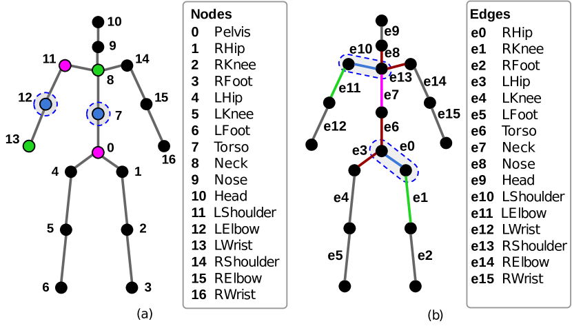
Figure 1: Graph representation of the human body: (a) Node definitions with examples of neighbor groups of two nodes, highlighted by dotted circles. Blue, pink and green show the self, parent and child neighbors respectively. (b) Edge definitions and examples of neighbor groups of two edges, highlighted by dotted ellipses. Blue, pink, green and maroon highlight the self, parent, child and junction neighbors respectively.

III-C Neighbor Groups and Adaptive Adjacency

Following PoseGraphNet [1], we apply non-uniform graph convolution by means of neighbor-group specific kernels. It allows extraction of different features for different neighbor groups. We categorize the node neighbors into three groups - a) self, b) parent (closer to the root joint), and c) child (away from the root joint). The edge neighbors are divided into four groups - a) self, b) parent, c) child, and d) junction. Junction is a special neighbor group, where the neighboring edges do not have a parent-child relationship, but the graph splits into branches, e.g. RHip and LHip; RShouhlder, Neck and LShoulder. Fig. 1 shows the graph structure along with some sample nodes/edges and their corresponding neighbors.

Based on the neighbor groups, the output features of hidden layer $l$ are computed following Eq. 3

$$H_{v}^{l+1}=\sigma{(\sum_{g\in G}\tilde{A_{vg}}(TH_{e}P_{e}+H_{v}^{l})W_{vg}})$$ (3)

$$H_{e}^{l+1}=\sigma{(\sum_{g\in G}\tilde{A_{eg}}(T^{T}H_{v}P_{v}+H_{e}^{l})W_{eg}})$$

where $G$ is the set of neighbor groups, $\tilde{A_{g}}$ contains the neighbor connections of neighbor group $g$, and $W_{g}$ is the trainable weight specific to group $g$. The degree normalized adjacency matrix $\tilde{A}$ in Eq. 2 enforces equal contribution by each neighbor. But, adaptive adjacency matrices will allow learning different contribution rates for different neighbors. So we also learn the adjacency matrices, following [1]. Additionally, as shown in [1], it will also help in learning long-range relationships between distant nodes or edges.

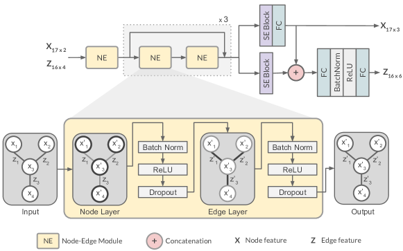
Figure 2: PoseGraphNet++ architecture. (top) Overall structure of the network. The residual block shown with a dotted box is repeated thrice. (bottom) Expanded view of the proposed Node-Edge module, showing the node and edge convolution layers.

III-D Rotation Representations

Rotations from SO(3) can be parameterized in multiple ways, e.g. with euler angles, unit quaternions or rotation matrices. Each has their own characteristics and their suitability for deep learning vary accordingly [41]. Euler angle representation suffers from ambiguity. Unit quaternions represent unique rotations, when restricted to a single hemisphere, but they are non-continuous in Euclidean space, leading to sub-optimal performance during training. Rotation matrices also represent unique rotations. However, there is a need to verify the orthogonality of the predicted rotation matrix, by either enforcing orthogonality regularization or normalization layer [41]. Zhou et al. [41] propose a novel 6D embedding of rotations, which is continuous in Euclidean space. They empirically demonstrate that the use of a continuous representation leads to better performance and stable results. The 6D representation is achieved by dropping the last column $\mathbf{r}_{3}$ of an orthogonal rotation matrix $R=[\mathbf{r}_{1}\ \mathbf{r}_{2}\ \mathbf{r}_{3}]$. i.e. $R_{6D}=[\mathbf{r}_{1}\ \mathbf{r}_{2}]$. The rotation matrix can be recovered by orthogonalizaton and normalization, specifically by $\mathbf{r^{\prime}}_{1}=\phi{(\mathbf{r}_{1}})$, $\mathbf{r^{\prime}}_{2}=\phi{(\mathbf{r}_{2}-(\mathbf{r^{\prime}}_{1}\cdot\mathbf{r}_{2})\mathbf{r^{\prime}}_{1})}$, and $\mathbf{r^{\prime}}_{3}=\mathbf{r^{\prime}}_{1}\times\mathbf{r^{\prime}}_{2}$, where $\phi$ denotes the vector normalization operation. For bone rotations we choose the 6D representation, due to its stable performance during training.

III-E Architecture

PoseGraphNet++ consists of 3 residual blocks, where each block consists of two node-edge (NE) modules. A NE module consists of a node and an edge layer, as defined in sec. III-B. The detailed architecture is described in Fig. 2. Each of the convolutional layers in NE is followed by a batch normalization layer, a ReLU activation and a dropout. A residual connection is added from the block input to the block output. The residual blocks are preceded by a NE module and succeeded by two downstream modules - the position head and the orientation head. Both downstream heads contain a Squeeze and Excitation (SE) Block [8], followed by one or more fully connected layers. The SE blocks re-calibrates the channel-wise features, following Eq. 4.

$$X^{\prime}=X\odot\mathrm{sigmoid}(W_{ex}\mathrm{relu}(W_{sq}X))$$ (4)

where $X$ and $X^{\prime}$ are the input and output of the SE Block, $W_{ex}\in R^{C\times\frac{C}{d}}$ is the excitation weight, $W_{sq}\in R^{\frac{C}{d}\times C}$ is the squeeze weight and $d$ is the squeeze ratio. The predicted joint positions from the position head are fed to the orientation head. The concatenated feature is passed to a linear layer, followed by a batch normalization, ReLU and a final linear layer, that produces the bone orientations.

III-F Loss Functions

The goal of our model is to learn joint locations and bone orientations from the 2D human pose. Eq. 5 shows the Mean Per Joint Position Error (MPJPE) loss function for joint locations that computes the mean squared error between the predicted and the ground truth joint positions.

$$L_{MPJPE}(J^{pred},J^{gt})=\frac{1}{N}\sum_{i=1}^{N}||J^{pred}_{i}-J^{gt}_{i}||_{2}^{2}$$ (5)

where $J^{pred}$ and $J^{gt}$ are the predicted and ground truth 3D joints respectively. We explore two loss functions to learn the bone orientations: the Identity deviation (IDev) loss [9] and the PLoss [31]. The IDev loss computes the distance of the product of the predicted and the transposed ground truth rotation matrix from the Identity matrix. For two identical rotation matrices, the distance should be zero. IDev is formally defined as:

$$L_{IDev}(R^{pred},R^{gt})=\frac{1}{N}\sum_{i=1}^{N}||I-R^{T}_{i,gt}R_{i,pred}||_{2}$$ (6)

where $R^{pred}$ and $R^{gt}$ are the predicted and ground truth rotation matrices. PLoss [31] computes the distance between a vector transformed by two rotations and is defined as:

$$L_{PLoss}(R^{pred},R^{gt})=\frac{1}{N}\sum_{i=1}^{N}||R_{i,pred}\hat{X}-R_{i,gt}X||_{1}$$ (7)

where $\hat{X}$ and $X$ are the predicted and ground truth joint locations. Empirically, we found that using the L1 norm instead of the L2 yielded better results. The final loss function $L$ is defined as $L=L_{MPJPE}+\lambda L_{Angle}$, where $L_{Angle}$ is either $L_{IDev}$ or $L_{Ploss}$, and $\lambda$ denotes the weight of $L_{Angle}$. For both IDev and PLoss we convert the predicted 6D rotation to a rotation matrix before computing the error.

IV Experiments

IV-A Datasets

Human3.6M [10] is a standard dataset for 3D human pose estimation task. It contains 3.6 million images of 7 subjects, from 4 different viewpoints performing 15 actions such as walking, sitting, etc. 2D locations in image space, 3D ground truth positions in camera space, and parent-relative bone orientations are available. The zero rotation pose follows the standard Vicon rest pose [7] (see supplementary materials.) As per the standard protocol [20, 3, 32, 37], we use subjects 1, 5, 6, 7, and 8 for training, and subjects 9 and 11 for evaluation.

MPI-3DHP Dataset [21] contains 3D poses in both indoor and outdoor scenes, but no ground truth rotation annotations are available. Hence, we only use this dataset to test the position error of our proposed model.

MPI-3DPW Dataset [29] contains annotations for 6D poses in-the-wild. The dataset utilizes the SMPL statistical model [18] for extracting the ground truth pose, which has a different skeletal structure than that of Human3.6M. We use the SMPL joint regressor to obtain the 2D and 3D joint locations in Human3.6M format. The zero rotation pose in this dataset is a T-Pose, unlike Human3.6M.

IV-B Metrics

Following previous work [1, 32, 7, 34], we compute Mean Per Joint Position Error (MPJPE) for evaluating the joint position prediction using two protocols: P1 and P2. As per P1, it is computed as the mean Euclidean distance of the predicted 3D joints to the ground truth joints in millimeters, as defined in Eq. 5. In P2 the predicted pose is aligned with the ground truth using Procrustes alignment before computing the error. To evaluate the performance of bone orientation prediction, we use two angular metrics - Mean Per Joint Angular Error (MPJAE) and Mean Average Accuracy (MAA). MPJAE [10] is the average geodesic distance $\theta_{sep}$ between the predicted and ground truth bone orientations $R_{pred}$ and $R_{gt}$ respectively, and ranges in $[0,\pi]$ radian. MAA [7] on the other hand is an accuracy metric. Formally, the metrics are defined as follows

$$MPJAE=\frac{1}{N}\sum_{i=1}^{N}\theta_{sep}(R_{i,gt},R_{i,pred})$$ (8)

$$MAA=\frac{1}{N}\sum_{i=1}^{N}1-\frac{\theta_{sep}(R_{i,gt},R_{i,pred})}{\pi}$$ (9)

where $\theta_{sep}(R_{i,gt},R_{i,pred})=||log(R^{T}_{i,gt}R_{i,pred})||_{2}$. The objective is to have lower MPJAE and higher MAA.

IV-C Implementation Details

Data pre-processing: We normalize the 2D inputs so that the image width is scaled to $[-1,1]$. We use the camera coordinates for the 3D output and align the root joint i.e. the pelvis to the origin. The joint angles are provided in Euler (ZXY). After normalizing the angles to $[-180,180]$ degree, they are converted to rotation matrices and then to the 6D representation (as described in sec. III-D). We predict the joint positions relative to the root joint and the bone rotations relative to their parent. The global orientation of the root is excluded from the evaluation.

Protocol #1	Dir.	Disc.	Eat	Greet	Phone	Photo	Pose	Purch.	Sit	SitD.	Smoke	Wait	WalkD.	Walk	WalkT.	Avg.
Martinez et al. [20] ICCV‘17	51.8	56.2	58.1	59.0	69.5	78.4	55.2	58.1	74.0	94.6	62.3	59.1	65.1	49.5	52.4	62.9
Cai et al. [3] ICCV‘19	46.5	48.8	47.6	50.9	52.9	61.3	48.3	45.8	59.2	64.4	51.2	48.4	53.5	39.2	41.2	50.6
Zhao et al. [36] CVPR‘19	47.3	60.7	51.4	60.5	61.1	49.9	47.3	68.1	86.2	55.0	67.8	61.0	42.1	60.6	45.3	57.6
Pavllo et al [25] CVPR‘19	47.1	50.6	49.0	51.8	53.6	61.4	49.4	47.4	59.3	67.4	52.4	49.5	55.3	39.5	42.7	51.8
Xu et al. [32] CVPR’21	45.2	49.9	47.5	50.9	54.9	66.1	48.5	46.3	59.7	71.5	51.4	48.6	53.9	39.9	44.1	51.9
Zhao et al. [37] CVPR’21	45.2	50.8	48.0	50.0	54.9	65.0	48.2	47.1	60.2	70.0	51.6	48.7	54.1	39.7	43.1	51.8
Banik et al. [1] ICIP’21	48.0	52.4	52.8	52.7	58.1	71.1	51.0	50.4	71.8	78.1	55.7	53.8	59.0	43.0	46.8	56.3
Ours	48.9	50.1	46.7	50.4	54.6	63.0	48.8	47.9	64.1	68.6	50.5	48.7	53.9	39.3	42.2	51.7
Protocol #2	Dir.	Disc.	Eat	Greet	Phone	Photo	Pose	Purch.	Sit	SitD.	Smoke	Wait	WalkD.	Walk	WalkT.	Avg.
Martinez et al. [20] ICCV‘17	39.5	43.2	46.4	47.0	51.0	56.0	41.4	40.6	56.5	69.4	49.2	45.0	49.5	38.0	43.1	47.7
Cai et al. [3] ICCV‘19	36.8	38.7	38.2	41.7	40.7	46.8	37.9	35.6	47.6	51.7	41.3	36.8	42.7	31.0	34.7	40.2
Pavllo et al [25] CVPR‘19	36.0	38.7	38.0	41.7	40.1	45.9	37.1	35.4	46.8	53.4	41.4	36.9	43.1	30.3	34.8	40.0
Zhao et al. [37] CVPR’22	41.6	45.3	46.7	46.8	51.3	56.5	43.6	43.7	56.1	62.0	50.9	46.0	50.1	39.2	45.0	48.3
Banik et al. [1] ICIP’21	36.6	41.5	41.6	42.3	43.9	52.0	39.4	38.7	56.2	61.4	44.4	41.2	48.0	33.9	38.9	44.0
Ours	38.9	39.0	37.1	40.6	40.9	46.9	37.0	35.9	50.9	54.6	40.3	36.7	41.4	30.4	34.9	40.2

TABLE I: Mean Per Joint Position Error (MPJPE) in millimeter on Human3.6M dataset under Protocol #1 (P1) and Protocol #2 (P2). CPN [4] predicted 2D keypoints are used as input. Lower MPJPE indicates better performance. The best scores are highlighted in bold.

Training details: We train our model on the Human3.6M dataset using the Adam optimizer for 20 epochs, using a batch size of 256, and a dropout rate of 0.2. The learning rate is initialized to 0.0001, and it is decayed by 0.92 after every 5 epochs. We use 256 channels in both node and edge layers of PoseGraphNet++. For the baseline model the MPJPE and the IDev loss are used. The hyperparameters $\lambda$ and the squeeze ratio $d$ are set to 20 and 8 empirically. The SoA SMPL-based methods [16, 12, 14] predict bone orientation with respect to T-pose. In contrast, PoseGraphNet++ trained on the original Human3.6M annotation predicts the orientation with respect to Vicon’s rest pose. To be able to compare these methods, we train PoseGraphNet++ also on the annotations provided by [16], which contain the ground truth orientation in the SMPL format. Due to fewer samples in this annotation, we train longer (70 epochs) with batch size 32. PoseGraphNet++ trained on the Human3.6M T-pose annotations is named as PoseGraphNet++ (T-pose).

IV-D Experimental Results

In this section, we report the position, orientation and joint-wise errors of our baseline model, which is trained on the train set of Human3.6M. Following the SoA methods [1, 32, 37], we use the noisy 2D joint predictions by Cascaded Pyramid Network (CPN) [4] as the input node features. For the bone features, the 2D bone rotations derived from the joint positions are used. To validate the generalization performance of our model, we also evaluate on the MPI-3DHP and MPI-3DPW datasets.

Position Evaluation: We evaluate the predicted positions using the MPJPE metric on Human3.6M test set. The P1 and P2 MPJPE scores for the 15 actions in Human3.6M dataset are reported in Tab. I along with the scores of the SoA methods. We do not consider image- and video-based 3D pose methods here, since they have the advantage of additional image or temporal features. PoseGraphNet++ achieves a mean MPJPE of $51.7$ mm in P1 and $40.2$ mm in P2. As can be seen in Tab. I, the performance of our model is close to the SoA performance of $50.6$ mm [3]. On 9 out of 15 actions our model’s performance is one of the top 3 performances. PoseGraphNet++ has 4.6M model parameters, and achieves an inference time of 5.37ms using Nvidia Tesla T4 GPU, in contrast to 13.1 ms by its closest competitor GraFormer [37] with 0.65M parameters.

	Position		Orientation
Method	P1 $\downarrow$	P2 $\downarrow$	MPJAE $\downarrow$	MAA $\uparrow$
SPIN [14]	54.88	36.65	0.20	93.58
HybrIK-ResNet (3DPW) [16]	50.22	32.38	0.30	90.43
HybrIK-HRNet (w/o 3DPW) [16]	44.97	27.46	0.24	92.28
Skeleton2Mesh* [34]	87.1	55.4	0.39	-
OKPS+ [7]	47.4	36.1	0.21	93.20
Ours (T-Pose)	50.60	37.21	0.23	92.78
Ours (T-Pose)*	50.60	37.21	0.21	93.34

TABLE II: Position and orientation performance of PoseGraphNet++ (T-pose) on Human3.6M along with SoA. $*$ and ⁺ indicate orientation evaluation is performed on ten joints following [34], and including global orientation following [7] respectively.

Orientation Evaluation: To the best of our knowledge, PoseGraphNet++ is the first skeletal-based human pose estimation method that predicts both joint position and bone rotations. We compare our method with SMPL-based methods [14, 16, 34] and OKPS [7], as they predict both position and orientation. Most of the SoA methods only report position error. In an effort to compare our model with the SoA, we evaluate the open-source models [14, 16] for their orientation performance following our evaluation setup, which excludes the root joint. Unlike the other SoA methods, OKPS [7] and Skeleton2Mesh [34] evaluate the orientation on a limited set of joints. For a fair comparison, we re-evaluate our method on the same joints as Skeleton2Mesh as defined in [34]. Unfortunately, this could not be pursued for OKPS, as they do not provide the exact details of the joints. We report the position and orientation performance of PoseGraphNet++ (T-pose) (refer sec. IV-C) and the SoA on Human3.6M test set in Tab. II.

Our method achieves 50.6 mm MPJPE and 0.23 rad MPJAE. PoseGraphNet++ (T-pose) is the third best model in terms of orientation error, lagging behind the best performing model SPIN [14] only by $0.03$ rad. Note, the second best model is OKPS, which is evaluated on a different set of joints including the root joint, and therefore is not comparable. Our positional performance is also on par with the SMPL-based methods, outperforming SPIN [14] and Skeleton2Mesh [34], and being very close to HybrIK-ResNet [16]. HybrIK-HRNet achieves lower position error as their HRNet predicted input pose is more accurate [26].

PoseGraphNet++ only relies on the predicted 2D pose and orientation and no additional image feature, unlike the others. Skeleton2Mesh is the closest to our method in this sense, as they also infer the joint angles only from a 2D skeleton. However, our method outperforms it by a large margin. Our results show that like 2D-to-3D pose lifting methods, it is possible to infer bone orientations from 2D poses by exploiting 2D joint and bone features and the structural bias of the skeleton. Even roll, which is unobserved in the input 2D pose, can be recovered. The yaw, roll and pitch errors are 0.11, 0.13 and 0.13 rad respectively. Similar to the action-level positional errors, the highest orientation error occurs for the actions involving sitting for example Photo and Sitting Down (0.26 and 0.29 radian respectively).

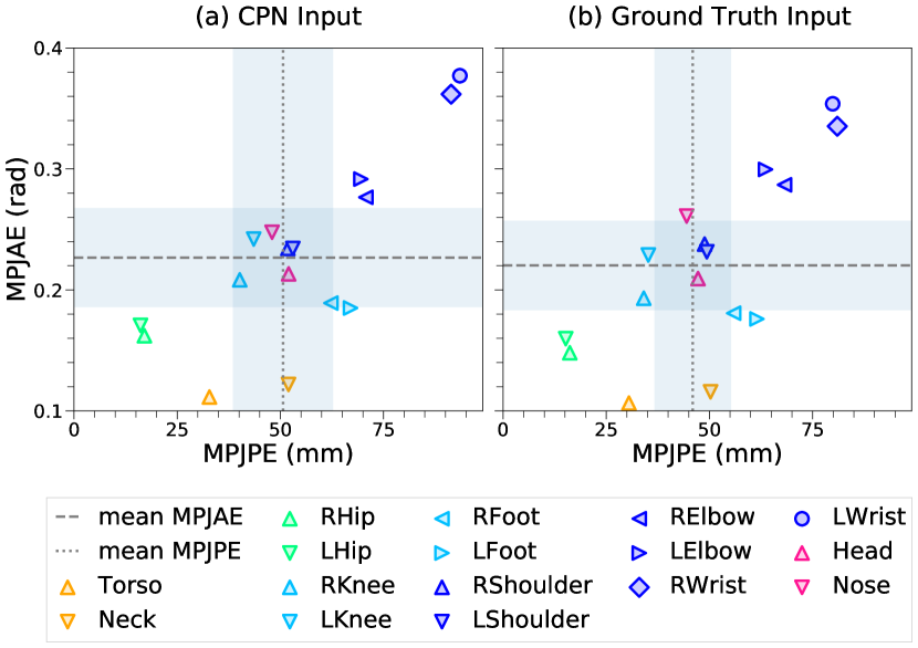
Figure 3: Joint-wise MPJAE vs MPJPE on Human3.6M test set using (a) CPN predictions, (b) 2D ground truth. The dotted lines and the shaded area denote the mean errors and one standard deviation respectively. Joints belonging to the same body part are shown with same color and are distinguished by different symbols.

Joint-wise Error Analysis: We plot the joint-wise MPJPE and MPJAE scores on Human3.6M test set for CPN predicted noisy input in Fig. 3 (a), and for the ground truth input data in Fig. 3 (b). The mean and the standard deviation in both metrics are higher for the CPN-predicted input. The majority of the errors occur for the joints wrists and elbows, and additionally for feet in case of positional error. The positional variance for these joints are higher in this dataset, which leads to high errors. The shoulders, knees and joints belonging to the torso region are the most stable ones, which is also evident in their low positional and orientation errors. With more accurate 2D input, the performance will increase, as can be seen in Fig. 3 (b). Also, temporal data will help to recover from the effect of the noisy input.

Generalization performance: To test the generalization ability of our model on other datasets, we evaluate our model on MPI-3DHP and MPI-3DPW test sets. Following [20, 37], we report the position metrics 3DPCK and AUC on 3DHP test set in Tab. III. Both of our models outperform the SoA methods on 3DHP test set in terms of 3DPCK, showing the generalization capabilities of the model. For AUC, PoseGraphNet++ performs the best, closely followed by PoseGraphNet++ (T-pose).

Methods	3DPCK $\uparrow$	AUC $\uparrow$
Martinez (H36M) [20]	42.5	17.0
Mehta (H36M) [21]	64.7	31.7
Yang (H36, MPII) [33]	69.0	32.0
Zhou (H36M, MPII) [40]	69.2	32.5
Luo (H36M) [19]	65.6	33.2
Ci (H36M) [5]	74.0	36.7
Zhou (H36M, MPII) [39]	75.3	38.0
Zhao (H36M) [37]	79.0	43.8
Xu (H36M) [32]	80.1	45.8
Ours	81.1	46.6
Ours (T-Pose)	80.2	44.4

TABLE III: 3DPCK and AUC on 3DHP test set. Our models are trained on Human3.6M. The best and the second best scores are highlighted with bold and underline. Higher scores are better.

Methods	MPJPE $\downarrow$	PMPJPE $\downarrow$	MPJAE $\downarrow$
HybrIK HRNet [16] (COCO, 3DHP, H3.6m)	88.00	48.57	0.30
SPIN [14] (H3.6m, 3DHP, LSP, MPII, COCO)	94.17	56.20	0.30
OKPS+ (H3.6m, MPII) [7]	115.40	76.70	0.41
Ours (H36M)	104.96	55.30	0.30

TABLE IV: MPJPE (mm) and MPJAE (rad) on 3DPW test set. Lower scores are better. ⁺ denotes including global orientation. Best scores are highlighted in bold.

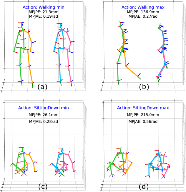
Figure 4: Qualitative results on Human3.6M test set for two actions with noisy CPN inputs. Each plot shows the ground truth skeleton on the left and the predicted one on the right. (a,c) and (b,d) show the best and failure cases respectively.

We evaluate only our PoseGraphNet++ (T-pose) model on the 3DPW dataset, as the orientations annotations in this dataset are with respect to T-pose. Tab. IV reports the position and the orientation errors of our Human3.6M trained model on 3DPW. Our method shows good generalization capability to this unseen dataset as well. OKPS performs the worst in terms of MPJPE. Their orientation error includes the global orientation, and therefore it cannot be compared with others. Though our method lags behind the SMPL-based methods in terms of positional performance by 20%, the orientation error is the same. Our bone orientation estimation is as good as the SMPL-based methods, although we use only 2D pose as input.

Fig. 4 shows samples with minimum and maximum MPJPE error for two actions Walking and Sitting down. For the best case scenarios (a, c), the overall 6D pose could be recovered with some minor discrepancies (note the head orientation and the roll of the left arm in Fig. 4 (c)). We observe that the leg pose could not be recovered for the side view example in Fig. 4 (b). This problem is due to the incorrect 2D prediction made by CPN and does not occur when the ground truth 2D pose is used as input. See supplementary materials for more examples from all datasets.

IV-E Ablation Study

We conduct several experiments to understand the impact of node-edge convolution, the significance of multi-task learning, the effect of the loss functions, and the adjacency matrices. For the multi-task learning and loss experiments, PoseGraphNet++ is trained on the ground truth 2D joints.

	H36M		3DHP
Model	MPJPE $\downarrow$	MPJAE $\downarrow$	PCK $\uparrow$	AUC $\uparrow$
Node	52.6	0.27	75.2	39.5
Node+Edge	51.7	0.26	81.1	46.6

TABLE V: MPJPE and MPJAE score of Node-only and Node-Edge models on Human3.6M and 3DHP datasets.

Effect of Node-Edge convolution: To test the utility of Node-Edge (NE) convolutions, we compare with a Node-only (NN) model. We change all edge layers to node layers and train using the concatenated node and edge features as input. The NE model performs better than the NN model on Human3.6M and especially on 3DHP (see Tab. V). The NE model learns the relationships between the joint positions and orientations accurately, and thus generalizes better.

	Loss functions	MPJPE (mm) $\downarrow$	MPJAE (rad) $\downarrow$
(a)	MPJPE	38.92 $\pm$ 10.69	2.20 $\pm$ 0.10
	Identity Deviation	448.10 $\pm$ 26.08	0.25 $\pm$ 0.06
(b)	MPJPE + Identity Deviation	38.75 $\pm$ 11.13	0.22 $\pm$ 0.05
(c)	MPJPE + PLoss	39.06 $\pm$ 12.12	0.24 $\pm$ 0.04

TABLE VI: MPJPE and MPJAE with standard deviation on Human3.6M dataset for different loss functions. Lower error is better.

Multi-task learning: The first study analyzes if it is beneficial to learn the position and the orientation simultaneously. For this purpose, we train the model for the individual tasks using either the positional loss MPJPE or the orientation loss IDev, and also for both tasks using both losses. The MPJPE and MPJAE scores are reported Tab. VI (sections a, b). The results show that when learning both tasks,the errors achieved are lower than that when learning the tasks individually. For example, the model achieves 0.22 rad MPJAE when trained on both tasks, compared to 0.25 radian for the orientation task. This indicates that PoseGraphNet++ benefits from multi-task learning.

Loss functions: We evaluate the performance of the loss functions - IDev and PLoss and report the results in Tab. VI (sections b, c). MPJPE + PLoss performs the worst according to both metrics.

Adjacency Matrices: In this experiment, we study the effect of using neighbor-group specific kernels and adaptive adjacency matrices. Tab. VII reports the MPJPE and MPJAE scores for static and adaptive adjacency matrices for neighbor-group specific kernels (split adjacency) and uniform kernels (basic adjacency). We observe that learning $A_{V}$ helps in improving the positional error significantly (see Tab. VII compare (a) with (c) and (b) with (d)). Learning $A_{E}$ on the other hand reduces the MPJAE marginally. However, it contributes to reducing the position error (compare (a) with (b), and (c) with (d) in Tab. VII). This again proves that PoseGraphNet++ benefits from utilizing the mutual relationships between edges and nodes. Similar to GraAttention [37], adaptive adjacency finds long-range dependencies between joints [1], which helps to improve the performance. The models with the split adjacency outperform their counterparts by a large margin due to their capability to extract richer neighbor-group-specific features.

Based on the conducted ablation studies, we chose the Node-Edge architecture, MPJPE + IDev loss, neighbor-group specific kernels and adaptive adjacency for the proposed PoseGraphNet++ model.

			Split Adjacency		Basic Adjacency
Exp.	$A_{V}$	$A_{E}$	MPJPE $\downarrow$	MPJAE $\downarrow$	MPJPE $\downarrow$	MPJAE $\downarrow$
(a)	Static	Static	60.2	0.27	113.2	0.32
(b)	Static	Adaptive	54.0	0.27	72.7	0.31
(c)	Adaptive	Static	52.2	0.27	82.2	0.30
(d)	Adaptive	Adaptive	51.7	0.26	79.2	0.30

TABLE VII: MPJPE and MPJAE on Human3.6M dataset for different adjacency matrices. $A_{V}$ and $A_{E}$ denote node and edge adjacency matrices.

V Conclusion and Future Work

We present the first skeletal-based human pose estimation model, PoseGraphNet++ for predicting the 3D position and orientation of joints simultaneously. Our results show that, like 3D positions, it is also possible to lift the 3D orientation from 2D poses by exploiting joint and bone features. We report both position and orientation errors on multiple benchmark datasets. Our model’s performance is close to the SoA methods on Human3.6M and MPI-3DPW datasets and is the best on MPI-3DHP. In the future, we would like to extend this work to spatio-temporal data to minimize the adverse effects of noisy input.

References

- [1] Soubarna Banik, Alejandro Mendoza GarcÍa, and Alois Knoll. 3D Human Pose Regression Using Graph Convolutional Network. In IEEE International Conference on Image Processing (ICIP), pages 924–928, Sept. 2021. ISSN: 2381-8549.
- [2] Federica Bogo, Angjoo Kanazawa, Christoph Lassner, Peter Gehler, Javier Romero, and Michael J. Black. Keep It SMPL: Automatic Estimation of 3D Human Pose and Shape from a Single Image. In European Conference on Computer Vision (ECCV), pages 561–578, Cham, 2016. Springer International Publishing.
- [3] Yujun Cai, Liuhao Ge, Jun Liu, Jianfei Cai, Tat-Jen Cham, Junsong Yuan, and Nadia Magnenat Thalmann. Exploiting Spatial-temporal Relationships for 3D Pose Estimation via Graph Convolutional Networks. In Proceedings of the IEEE International Conference on Computer Vision, 2019.
- [4] Yilun Chen, Zhicheng Wang, Yuxiang Peng, Zhiqiang Zhang, Gang Yu, and Jian Sun. Cascaded pyramid network for multi-person pose estimation. In Proceedings of the IEEE/CVF Conference on Computer Vision and Pattern Recognition, pages 7103–7112, 2018.
- [5] Hai Ci, Chunyu Wang, Xiaoxuan Ma, and Yizhou Wang. Optimizing Network Structure for 3D Human Pose Estimation. In Proceedings of the IEEE International Conference on Computer Vision, October 2019.
- [6] Bardia Doosti, Shujon Naha, Majid Mirbagheri, and David J Crandall. Hope-net: A graph-based model for hand-object pose estimation. In Proceedings of the IEEE/CVF Conference on Computer Vision and Pattern Recognition, pages 6608–6617, 2020.
- [7] Martin Adrian Fisch and Ronald Clark. Orientation keypoints for 6D human pose estimation. IEEE Transactions on Pattern Analysis and Machine Intelligence, 2021.
- [8] Jie Hu, Li Shen, and Gang Sun. Squeeze-and-excitation networks. In Proceedings of the IEEE/CVF Conference on Computer Vision and Pattern Recognition, pages 7132–7141, 2018.
- [9] Du Q Huynh. Metrics for 3D rotations: Comparison and analysis. Journal of Mathematical Imaging and Vision, 35(2):155–164, 2009.
- [10] Catalin Ionescu, Dragos Papava, Vlad Olaru, and Cristian Sminchisescu. Human3.6m: Large scale datasets and predictive methods for 3D human sensing in natural environments. IEEE Transactions on Pattern Analysis and Machine Intelligence, 36(7):1325–1339, 2013.
- [11] Xiaodong Jiang, Ronghang Zhu, Sheng Li, and Pengsheng Ji. Co-embedding of nodes and edges with graph neural networks. IEEE Transactions on Pattern Analysis and Machine Intelligence, 2020.
- [12] Angjoo Kanazawa, Michael J. Black, David W. Jacobs, and Jitendra Malik. End-to-end Recovery of Human Shape and Pose. In Proceedings of the IEEE/CVF Conference on Computer Vision and Pattern Recognition, 2018.
- [13] Thomas N. Kipf and Max Welling. Semi-Supervised Classification with Graph Convolutional Networks. In International Conference on Learning Representations, ICLR, Toulon, France, April 24-26, 2017, Conference Track Proceedings. OpenReview.net, 2017.
- [14] Nikos Kolotouros, Georgios Pavlakos, Michael J Black, and Kostas Daniilidis. Learning to reconstruct 3d human pose and shape via model-fitting in the loop. In Proceedings of the IEEE International Conference on Computer Vision, 2019.
- [15] Nikos Kolotouros, Georgios Pavlakos, and Kostas Daniilidis. Convolutional mesh regression for single-image human shape reconstruction. In Proceedings of the IEEE/CVF Conference on Computer Vision and Pattern Recognition, pages 4501–4510, 2019.
- [16] Jiefeng Li, Chao Xu, Zhicun Chen, Siyuan Bian, Lixin Yang, and Cewu Lu. Hybrik: A hybrid analytical-neural inverse kinematics solution for 3d human pose and shape estimation. In Proceedings of the IEEE/CVF Conference on Computer Vision and Pattern Recognition, pages 3383–3393, 2021.
- [17] Kenkun Liu, Rongqi Ding, Zhiming Zou, Le Wang, and Wei Tang. A comprehensive study of weight sharing in graph networks for 3D human pose estimation. In European Conference on Computer Vision (ECCV), pages 318–334. Springer, 2020.
- [18] Matthew Loper, Naureen Mahmood, Javier Romero, Gerard Pons-Moll, and Michael J. Black. SMPL: a skinned multi-person linear model. ACM Transactions on Graphics, 34(6):1–16, Nov. 2015.
- [19] Chenxu Luo, Xiao Chu, and Alan Yuille. OriNet: A Fully Convolutional Network for 3D Human Pose Estimation. In Proceedings of the British Machine Vision Conference (BMVC), 2018.
- [20] Julieta Martinez, Rayat Hossain, Javier Romero, and James J Little. A simple yet effective baseline for 3D human pose estimation. In Proceedings of the IEEE International Conference on Computer Vision, 2017.
- [21] Dushyant Mehta, Helge Rhodin, Dan Casas, Pascal Fua, Oleksandr Sotnychenko, Weipeng Xu, and Christian Theobalt. Monocular 3D Human Pose Estimation In The Wild Using Improved CNN Supervision. In 3D Vision (3DV), 2017 Fifth International Conference on. IEEE, 2017.
- [22] Georgios Pavlakos, Vasileios Choutas, Nima Ghorbani, Timo Bolkart, Ahmed A. A. Osman, Dimitrios Tzionas, and Michael J. Black. Expressive body capture: 3d hands, face, and body from a single image. In Proceedings of the IEEE/CVF Conference on Computer Vision and Pattern Recognition, 2019.
- [23] Georgios Pavlakos, Xiaowei Zhou, and Kostas Daniilidis. Ordinal Depth Supervision for 3D Human Pose Estimation. Proceedings of the IEEE/CVF Conference on Computer Vision and Pattern Recognition, 2018.
- [24] Georgios Pavlakos, Xiaowei Zhou, Konstantinos G Derpanis, and Kostas Daniilidis. Coarse-to-fine volumetric prediction for single-image 3D human pose. In Proceedings of the IEEE/CVF Conference on Computer Vision and Pattern Recognition, pages 7025–7034, 2017.
- [25] Dario Pavllo, Eth Zürich, Christoph Feichtenhofer, David Grangier, Google Brain, and Michael Auli. 3D human pose estimation in video with temporal convolutions and semi-supervised training. In Proceedings of the IEEE/CVF Conference on Computer Vision and Pattern Recognition, 2019.
- [26] Ke Sun, Bin Xiao, Dong Liu, and Jingdong Wang. Deep high-resolution representation learning for human pose estimation. In Proceedings of the IEEE/CVF conference on computer vision and pattern recognition, pages 5693–5703, 2019.
- [27] Bugra Tekin, Isinsu Katircioglu, Mathieu Salzmann, Vincent Lepetit, and Pascal Fua. Structured Prediction of 3D Human Pose with Deep Neural Networks. In Proceedings of the British Machine Vision Conference (BMVC), pages 130.1–130.11. BMVA Press, September 2016.
- [28] Denis Tome, Chris Russell, and Lourdes Agapito. Lifting from the deep: Convolutional 3D pose estimation from a single image. In Proceedings of the IEEE/CVF Conference on Computer Vision and Pattern Recognition, pages 2500–2509, 2017.
- [29] Timo von Marcard, Roberto Henschel, Michael Black, Bodo Rosenhahn, and Gerard Pons-Moll. Recovering Accurate 3D Human Pose in The Wild Using IMUs and a Moving Camera. In European Conference on Computer Vision (ECCV), sep 2018.
- [30] Yue Wang, Yongbin Sun, Ziwei Liu, Sanjay E Sarma, Michael M Bronstein, and Justin M Solomon. Dynamic graph CNN for learning on point clouds. ACM Transactions on Graphics, 38(5):1–12, 2019.
- [31] Yu Xiang, Tanner Schmidt, Venkatraman Narayanan, and Dieter Fox. PoseCNN: A Convolutional Neural Network for 6D Object Pose Estimation in Cluttered Scenes. Robotics: Science and Systems (RSS), 2018.
- [32] Tianhan Xu and Wataru Takano. Graph stacked hourglass networks for 3D human pose estimation. In Proceedings of the IEEE/CVF Conference on Computer Vision and Pattern Recognition, pages 16105–16114, 2021.
- [33] Wei Yang, Wanli Ouyang, X. Wang, Jimmy S. J. Ren, Hongsheng Li, and Xiaogang Wang. 3D Human Pose Estimation in the Wild by Adversarial Learning. Proceedings of the IEEE/CVF Conference on Computer Vision and Pattern Recognition, pages 5255–5264, 2018.
- [34] Zhenbo Yu, Junjie Wang, Jingwei Xu, Bingbing Ni, Chenglong Zhao, Minsi Wang, and Wenjun Zhang. Skeleton2Mesh: Kinematics Prior Injected Unsupervised Human Mesh Recovery. In Proceedings of the IEEE/CVF International Conference on Computer Vision, pages 8619–8629, 2021.
- [35] Hongwen Zhang, Yating Tian, Xinchi Zhou, Wanli Ouyang, Yebin Liu, Limin Wang, and Zhenan Sun. PyMAF: 3D Human Pose and Shape Regression with Pyramidal Mesh Alignment Feedback Loop. In Proceedings of the IEEE International Conference on Computer Vision, 2021.
- [36] Long Zhao, Xi Peng, Yu Tian, Mubbasir Kapadia, and Dimitris N Metaxas. Semantic Graph Convolutional Networks for 3D Human Pose Regression. In Proceedings of the IEEE/CVF Conference on Computer Vision and Pattern Recognition, 2019.
- [37] Weixi Zhao, Weiqiang Wang, and Yunjie Tian. GraFormer: Graph-Oriented Transformer for 3D Pose Estimation. In Proceedings of the IEEE/CVF Conference on Computer Vision and Pattern Recognition, pages 20438–20447, June 2022.
- [38] Jie Zhou, Ganqu Cui, Shengding Hu, Zhengyan Zhang, Cheng Yang, Zhiyuan Liu, Lifeng Wang, Changcheng Li, and Maosong Sun. Graph neural networks: A review of methods and applications. AI Open, 1:57–81, 2020.
- [39] Kun Zhou, Xiaoguang Han, Nianjuan Jiang, Kui Jia, and Jiangbo Lu. HEMlets Pose: Learning Part-Centric Heatmap Triplets for Accurate 3D Human Pose Estimation. Proceedings of the IEEE International Conference on Computer Vision, pages 2344–2353, 2019.
- [40] Xingyi Zhou, Qixing Huang, Xiao Sun, Xiangyang Xue, and Yichen Wei. Towards 3D Human Pose Estimation in the Wild: A Weakly-Supervised Approach. In Proceedings of the IEEE International Conference on Computer Vision, Oct 2017.
- [41] Yi Zhou, Connelly Barnes, Jingwan Lu, Jimei Yang, and Hao Li. On the continuity of rotation representations in neural networks. In Proceedings of the IEEE/CVF Conference on Computer Vision and Pattern Recognition, pages 5745–5753, 2019.