Integrability is attractive

Abstract

The interplay between quantum chaos and integrability has been extensively studied in the past decades. We approach this topic from the point of view of geometry encoded in the quantum geometric tensor, which describes the complexity of adiabatic transformations. In particular, we consider two generic models of spin chains that are parameterized by two independent couplings. In one, the integrability breaking perturbation is global while, in the other, integrability is broken only at the boundary. In both cases, the shortest paths in the coupling space lead towards integrable regions and we argue that this behavior is generic. These regions thus act as attractors of adiabatic flows similar to river basins in nature. Physically, the directions towards integrable regions are characterized by faster relaxation dynamics than those parallel to integrability. The anisotropy between them diverges in the thermodynamic limit as the system approaches the integrable point. As side results, we provide evidence that the transition from integrable to chaotic behavior is universal for both models, similar to continuous phase transitions, and that the model with local integrability breaking quickly becomes chaotic but avoids ergodicity even in the thermodynamic limit.

I Introduction

There has been significant progress in understanding the nature of quantum chaos and integrability in the past few decades (see Refs. [1, 2, 3, 4, 5] for review). On one hand, it is generally recognized that the random matrix behavior of quantum eigenstates and energy spectrum are sensible measures of quantum chaos or, more accurately, quantum ergodicity [6, 7]. Emergent random matrix ensembles are connected with statistical mechanics and thermodynamics via the so-called eigenstate thermalization hypothesis (ETH) [8, 9, 5]. On the other hand, Poisson statistics of the level spacings is considered a signature of quantum integrability through the Berry-Tabor conjecture [10]. From the point of view of physical observables, integrable systems are generally non-ergodic with their steady states being constrained by multiple conservation laws. In systems with local interactions, these states can be described by the so-called generalized Gibbs ensemble (GGE) [11]. In weakly nonintegrable systems, it is generally expected that these states first relax to such GGE states and then gradually relax to a true equilibrium. This slow relaxation mechanism is termed prethermalization [12, 13, 5, 14].

Figure 1: Schematic representation of the adiabatic flows in 2D parameter space. The two horizontal blue lines represent the lines of integrability while the regions outside them are chaotic. The horizontal (vertical) axis represents the integrability preserving (breaking) direction. By following the minimal $\chi$-directions, we can construct the shortest paths or flows (solid gray lines) that tend towards the integrable lines. The plot is based on the XXZ spin analyzed in this work.

A different approach for analyzing the transition between quantum chaos and integrability, which is more relevant to the present work, is based on the scaling analysis of the fidelity susceptibility $\chi$ as a function of integrability breaking perturbations [15, 16, 17, 18, 19]. This approach was previously developed to study quantum phase transitions [20, 21, 22], allowing one to classify universal properties of quantum phases and phase transitions in an observable-independent way. When applied to excited states, fidelity susceptibility, together with other probes, enables one to identify the existence of a chaotic but non-ergodic buffer region that generically separates integrable and ergodic regimes. This buffer zone is characterized by a maximally divergent fidelity susceptibility and divergent relaxation times [17, 23, 15, 16]. It was recognized that, at or near integrable points, there is a strong qualitative difference between the dynamics of integrability preserving and integrability breaking perturbations [17, 24]. If we deal with more than one coupling, then fidelity susceptibilities are the diagonal parts of the full quantum geometric tensor (QGT). The QGT defines a natural Riemannian metric structure on the eigenstate manifolds  [25, 21, 22]. While the definition of QGT sounds abstract, it is closely related to the long time response of physical observables [26], quantum Fisher information [27], quantum speed limits [28, 29], effective mass [26], superfluidity and superconductivity [30], and various other physical phenomena (see Ref. [26] for details).

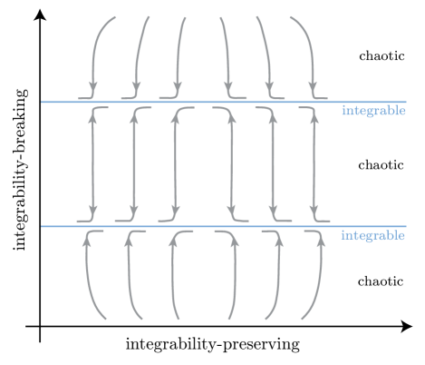
In this work, we analyze the properties of the QGT in two models, which have both integrable and chaotic regimes. At each point in the coupling space, we diagonalize the QGT and find the two orthogonal directions that maximize and minimize the fidelity susceptibilities. We then follow the minimal norm direction by infinitesimally changing the couplings and rediagonalizing the metric tensor to update this direction. From this, we obtain the flow lines similar to geodesics. This work extends that of Ref. [31] with the crucial difference that we used the norm of the full metric, not that of an approximate local adiabatic gauge potential. The latter is generally not sensitive to neither integrability nor long time relaxation. The key finding of our work is schematically illustrated in Fig. 1. Namely, we observe that integrable regions are the attractors of these flows. In other words, if we follow the minimal $\chi$-directions, we will reach regions of integrability (if they exist) as the flows abruptly turn their directions to stay within the integrable regions. Physically, the minimal $\chi$-directions correspond to the fastest relaxation dynamics of the observables conjugate to these directions. In the model with an extended integrability breaking perturbation, these fast observables avoid long prethermalization. In the model with a boundary integrability breaking term, we find that prethermalization is longer along the direction parallel to the integrability. Hence, we can reformulate our main result: following directions of fastest relaxation brings the system towards integrability. Additionally, we find universal scaling behavior of the fidelity susceptibilities along the fastest and the slowest directions, bearing close similarities between integrability breaking and critical behavior near continuous phase transitions.

II QGT and Fidelity Susceptibility

In this section, we give a brief introduction to the concepts of the quantum geometric tensor and the fidelity susceptibility and discuss their regularization such that they are well behaved in the thermodynamic limit. Much of the content here has been discussed in earlier papers (see Refs. [31, 17, 26] for further details), so we only mention details important for understanding the rest of this paper.

Suppose we have a Hamiltonian $\mathcal{H}({\bf\it\lambda})$ with coupling parameters ${\bf\it\lambda}=\{\lambda_{j}\}$. The (eigenstate averaged) quantum geometric tensor  is defined as

$$g_{ij}=\frac{1}{2\mathcal{D}}\sum_{n}\langle n|\mathcal{A}_{i}\mathcal{A}_{j}+\mathcal{A}_{j}\mathcal{A}_{i}|n\rangle_{c},$$ (1)

where $\mathcal{D}$ is the Hilbert space dimension , $|n\rangle$ is the ${\bf\it\lambda}$-dependent eigenstate of the Hamiltonian, and the subindex “c” stands for the connected part or the covariance: $\langle n|\mathcal{A}_{i}\mathcal{A}_{j}|n\rangle_{c}\equiv\langle n|\mathcal{A}_{i}\mathcal{A}_{j}|n\rangle-\langle n|\mathcal{A}_{i}|n\rangle\langle n|\mathcal{A}_{j}|n\rangle$. Here, $\mathcal{A}_{j}$ is the adiabatic gauge potential (AGP) in the $j$-th direction, defined as the derivative operator acting on the eigenstates of the Hamiltonian (we set $\hbar=1$):

$$i\partial_{\lambda_{j}}\ket{n({\bf\it\lambda})}=\mathcal{A}_{j}\ket{n({\bf\it\lambda})}\,,$$ (2)

The AGP and hence the QGT generally diverge in the thermodynamic limit and thus we consider their regularized version with the frequency cutoff $\mu$ [17]:

$$\matrixelement{m}{\mathcal{A}_{j}}{n}=-i\frac{\omega_{mn}}{\omega_{mn}^{2}+\mu^{2}}\matrixelement{m}{\partial_{j}\mathcal{H}}{n}\,,$$ (3)

where $\omega_{mn}\equiv\epsilon_{m}-\epsilon_{n}$ with $\epsilon_{n}$ and $\epsilon_{m}$ being the energy eigenvalues. In order to have a well defined self-averaging behavior of the QGT in the thermodynamic limit, $\mu$ needs to be chosen to be parametrically larger than the typical level spacing. Then, the regularized QGT reads

$$g_{ij}=\frac{1}{\mathcal{D}}\sum_{n,m}\frac{\omega_{nm}^{2}}{(\omega_{nm}^{2}+\mu^{2})^{2}}\langle m|\partial_{i}\mathcal{H}|n\rangle\langle n|\partial_{j}\mathcal{H}|m\rangle.$$ (4)

As in Ref. [17], we consider the regime $1/\mathcal{D}_{s}\ll\mu\ll\mathcal{O}(1)$ , where $\mathcal{D}_{s}$ is the Hilbert space dimension of the largest symmetry sector of the model and the upper bound frequency of order one is roughly located at the onset of relaxation. Depending on the model, this upper bound can weakly (polynomially) depend on the system size $L$, while $\mathcal{D}_{s}$ typically depends exponentially on $L$. Henceforth, we will refer to the limit $L\to\infty$ with $\mu$ satisfying the constraint above as the “effective” thermodynamic limit.

We focus on a two-dimensional control parameter space set by the couplings $h$ and $g$ (defined later for specific models) such that ${\bf\it\lambda}=(h,g)$. Let us observe that the AGP, as a derivative operator, transforms as a vector under rotations in the coupling space and hence the QGT transforms as a tensor. Suppose we have an infinitesimally small deformation such that ${\bf\it\lambda}+\differential{{\bf\it\lambda}}=(h+\differential{\lambda}\cos(\varphi),g+\differential{\lambda}\sin(\varphi))$. Then, the AGP along the direction ${\bf\it\lambda}$ is given by

$$\mathcal{A}_{\varphi}({\bf\it\lambda})=\mathcal{A}_{h}\cos(\varphi)+\mathcal{A}_{g}\sin(\varphi)\,.$$ (5)

Diagonalizing the QGT is therefore equivalent to finding the angles $\varphi_{\rm min}(h,g)$ and $\varphi_{\max}(h,g)=\varphi_{\rm min}(h,g)+\pi/2$ along which the fidelity susceptibilities

$$\chi_{\varphi}\equiv g_{\varphi\varphi}=\frac{1}{\mathcal{D}}\sum_{n}\langle n|\mathcal{A}_{\varphi}^{2}|n\rangle_{c}$$ (6)

take their minimal and maximal values. Following directions $\{\varphi_{\text{min}}(h,g)\}$, we can reach a new eigenstate at $(h+\delta\lambda\cos\varphi,g+\delta\lambda\sin\varphi)$ and obtain the adiabatic flow diagram as shown in Fig. 1.

III Flow Diagrams

Now we present our main numerical results obtained using exact diagonalization for two different models with regions of integrability and chaos. Then, we extrapolate these results to construct approximate infinite temperature flow diagrams in the thermodynamic limit.

The first model we consider is an XXZ spin chain of size $L-1$ with open boundary conditions coupled to a single spin at the boundary (coined as c-XXZ):

$$\begin{split}\mathcal{H}_{\text{c-XXZ}}&=\frac{1}{2}\sum^{L-2}_{i=2}\left[\sigma_{i}^{x}\sigma_{i+1}^{x}+\sigma_{i}^{y}\sigma_{i+1}^{y}+\Delta\sigma_{i}^{z}\sigma_{i+1}^{z}\right]\\ &+\frac{g}{2}\left(\sigma_{1}^{x}\sigma_{2}^{x}+\sigma_{1}^{y}\sigma_{2}^{y}+\Delta\sigma_{1}^{z}\sigma_{2}^{z}\right)+h\sigma_{1}^{z}\,,\end{split}$$ (7)

where $\Delta$ is the anisotropy, $h$ is the local z-magnetic field strength on the spin at site $1$, and $g$ is the boundary exchange strength between the spin at site $1$ and the XXZ spin chain. For all subsequent calculations, we set $\Delta=1.2$. Notably, when $g=1$, we have an XXZ spin chain of length $L$ with a boundary magnetic field. Since an XXZ spin chain is integrable and a local field on the boundary does not break its integrability [35, 36], this model is integrable along the line $g=1$. Furthermore, the c-XXZ model is trivially integrable along the line $g=0$, and in the limits $g\to\infty$ and $h\to\infty$. At finite couplings in regions outside of these two integrable lines, this model is expected to be chaotic as the $g$-exchange generically breaks integrability.

We also consider the Ising model with both transverse and longitudinal fields (LTFIM) with periodic boundary conditions

$$\mathcal{H}_{\text{LTFIM}}=\sum^{L}_{i=1}\sigma_{i}^{z}\sigma_{i+1}^{z}+g\sum^{L}_{i=1}\sigma^{x}_{i}+h\sum^{L}_{i=1}\sigma^{z}_{i}\,,$$ (8)

where $g$ and $h$ are the transverse and longitudinal field strengths, respectively. This model is integrable along two lines: $h=0$, as it maps to free fermions via the Jordan-Wigner transformation, and $g=0$, as it reduces to the classical Ising model. Finally, it is integrable at the point $h\to\infty$ and $g\to\infty$, as it becomes noninteracting. Outside of these regions, the model exhibits chaos [37].

In Figs. 2a and 2b, we show the flow diagrams for the c-XXZ model with $L=18$ and the Ising model with $L=20$, respectively. For the c-XXZ model, we consider the zero-magnetization sector, while we use the $k=\pi/2$ quasi-momentum sector for the Ising model. Similar to Ref. [17], we set $\mu=\alpha L/\mathcal{D}_{s}$, where $\alpha$ is a number chosen of the order of one to minimize finite size effects (see Sec. V for detailed discussions). Remarkably, we can identify integrable regions without knowing them a-priori as attractors of the flow lines, which become nearly orthogonal to the lines of integrability ($g=0,\,g=1$ for the c-XXZ model and $g=0,\,h=0$ for the Ising model) and then abruptly turn their directions after reaching integrability. As we explain below, these features become sharper with increasing system size and decreasing cutoff $\mu$. We also clearly see that the anisotropy between the two orthogonal directions increases (color darkens) near the integrable regions.

Figure 2: Flow diagrams. The paths that follow minimal $\chi$-directions are presented for the (a) coupled XXZ model with $L=18$ within the zero-magnetization sector and (b) nonintegrable Ising model with $L=20$ within the $k=\pi/2$ quasi-momentum sector. The regularizers $\mu=2L/\mathcal{D}_{s}\approx 7.4\times 10^{-4}$, where $\mathcal{D}_{s}=\binom{L}{L/2}$ is the dimension of the zero-magnetization sector, and $\mu=2.5\cdot L/\mathcal{D}_{s}\approx 9.5\times 10^{-4}$, where $\mathcal{D}_{s}=2^{L}/L$ is the dimension of each quasi-momentum sector, were used for the respective systems. Colors represent the anisotropy of $\chi$: the ratio of the $\chi_{\text{max}}$ in maximal direction over $\chi_{\text{min}}$ in the minimal direction. Along the line $g=0$ for both models, the anisotropy strongly diverges and its value is over the limits of the color bars shown.

Figure 3: Phase diagrams. Qualitative pictures of the phases that connect regions of integrability (denoted by colored regions) of the parameter space are shown for the (a) coupled XXZ model and (b) nonintegrable Ising model, both in the thermodynamic limit. The phases are denoted by A, B, and C. The integrable lines are shown as blue lines while the dashed lines serve as guidelines to denote the connectivity of integrable regions within phases. The white boundary lines in (b) signify the uncertainty of the phase boundaries due to the limits of our numerical calculations.

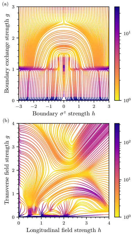
For the c-XXZ model, we can clearly identify two special points (vertices) on the integrable lines at $(h,g)=(0,0)$ and $(0,1)$. These are high degeneracy points, where, in addition to integrability, there are extra degeneracies due to the global $Z_{2}$ symmetry at $g=1$ and $Z_{2}\otimes SU(2)$ symmetry at $g=0$. Interestingly, we see that the $(0,1)$ vertex serves as an attractor of the adiabatic flows for $g<1$ but is repulsive for $g>1$. Similarly, $(0,0)$ is repulsive for $g>0$ and (though it is not shown) attractive for $g<0$. There are clearly also vertices at points $(|h|\to\infty,g=0)$ and $(|h|\to\infty,g=1)$, which can be also repulsive or attractive depending on which chaotic region they are in. For the Ising model, the flows near the whole integrable line $g=0$ become fragmented for $h\in(0,2)$ because this model has macrsocopic (exponential in the system size) degeneracies near rational values of $h$ in this interval, whose effects on the AGP were analyzed in Ref. [31]. Despite this fact, we can see that the line $g=0$ is still an attractor of the adiabatic flows. Moreover, as the system size increases, all singular behavior of the flows is pushed to lower values of $g$.

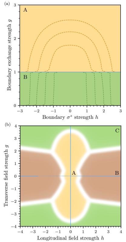
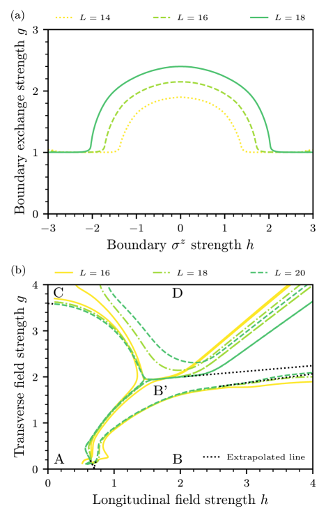
Now we do our best attempt to extrapolate the flow diagram to the thermodynamic limit by numerically examining trends of the flows for the coupled XXZ model with $L=14,16,18$ and nonintegrable Ising model with $L=16,18,20$, respectively (see Appendix A for more details). We identify boundaries separating the coupling space into distinct sectors, where, in each sector, the flows terminate at different integrable lines. The result of this extrapolation is shown in Figs. 3a and 3b. Note that there are no additional singularities near the lines separating different sectors except near integrable lines.

For the coupled XXZ model, there are two distinct sectors (denoted A and B) separated by the $g=1$ line that each connects different areas of integrability in the thermodynamic limit. Firstly, above the $g=1$ line, we have region A of paths that connect points $(\pm h,1)$ with curved arcs: that is, the shortest paths connect the integrable line $g=1$ with itself. Below the $g=1$ line, we have a distinct region B of almost vertical paths that connect the integrable lines $g=1$ and $g=0$. Finally, below the line $g=0$ line, there exists a region that connects the integrable line $g=0$ with itself (not shown in Fig. 3a).

For the nonintegrable Ising model, we find three regions denoted A, B, and C in the thermodynamic limit. Region A is characterized by paths that connect the integrable lines $h=0$ and $g=0$, B by paths that connect the integrable line $g=0$ with itself, and C by paths that connect integrable line $h=0$ with either the integrable point $\sqrt{h^{2}+g^{2}}\to\infty$ or line $g=0$. Since extrapolating precise form of the flows near the fragmented $g=0$ is difficult, we only extract the boundaries between the regions, which are robust and do not change much with the system size.

IV Universality of the Flows

In this section, we carefully analyze our numerical results presented in Sec. III, explaining their connection to prethermalization and universal long time relaxation of physical observables near the domains of integrability. In order to see why these domains act as attractors of adiabatic flows, let us rewrite $\chi_{\varphi}$ in terms of the Fourier transform of the spectral function $\Phi_{\varphi}(\omega)$ using Eq. (4):

$$\chi_{\varphi}({\bf\it\lambda})=\int^{\infty}_{-\infty}\differential{\omega}\frac{\omega^{2}}{(\omega^{2}+\mu^{2})^{2}}\Phi_{\varphi}(\omega)\,,$$ (9)

where

$$\Phi_{\varphi}(\omega)=\,\int^{\infty}_{-\infty}\frac{\differential{t}}{2\pi}e^{i\omega t}C_{\varphi}(t),$$ (10)

$$C_{\varphi}(t)\equiv\frac{1}{2\mathcal{D}}\sum_{n}\matrixelement{n}{\poissonbracket{\partial_{\varphi}\mathcal{H}(t)}{\partial_{\varphi}\mathcal{H}(0)}}{n}_{c}\,,$$ (11)

$\{\ldots\}$ is the anticommutator, $\matrixelement{n}{\partial_{\varphi}\mathcal{H}(t)\partial_{\varphi}\mathcal{H}(0)}{n}_{c}\equiv\matrixelement{n}{\partial_{\varphi}\mathcal{H}(t)\partial_{\varphi}\mathcal{H}(0)}{n}-\matrixelement{n}{\partial_{\varphi}\mathcal{H}(t)}{n}\matrixelement{n}{\partial_{\varphi}\mathcal{H}(0)}{n}$,

$$\partial_{\varphi}\mathcal{H}(t)\equiv e^{i\mathcal{H}t}\partial_{\varphi}\mathcal{H}e^{-i\mathcal{H}t}\,,$$ (12)

and $\partial_{\varphi}\mathcal{H}=\partial_{h}\mathcal{H}\cos(\varphi)+\partial_{g}\mathcal{H}\sin(\varphi)$.

Since Eq. (9) implies that $\chi_{\varphi}$ is dominated by low-frequency spectral weight, for small $\mu$ [17],

$$\chi_{\varphi}({\bf\it\lambda})\approx\begin{cases}\frac{\Phi_{\varphi}(\mu)}{\mu}&\text{if }\mu>\Delta\\ \frac{\Phi_{\varphi}(\Delta)}{\Delta}&\text{otherwise},\end{cases}$$ (13)

where $\Delta$ is the spectral gap. The angle $\varphi_{\rm min}$ ($\varphi_{\rm max}$) thus corresponds to the direction along which the spectral function takes the minimal (maximal) value.

For the Ising model at $h=0$, the spectral function vanishes at $\omega\to 0$ along the integrable direction $g$ due to the presence of a spectral gap leading to a small (polynomial in the system size) value of $\chi_{g}$ [17]. Conversely, along the integrability breaking $h$ direction, there are no selection rules for the matrix elements and the spectral function is constant at $\omega\to 0$ such that $\chi_{h}\sim 1/\mu$. Thus, we conclude that at $h=0$ we have $\varphi_{\rm min}={\pi/2}$, i.e. parallel to the $g$ direction, with $\chi_{\rm min}/\chi_{\rm max}\sim\mu\ll 1$. As we slightly increase $h$, the spectral function along the $h$ direction remains constant at small frequencies. Conversely, in the $g$ direction, it is easy to show using perturbation theory in $h$ that $\Phi_{g}(\omega)\sim h^{2}/\omega^{2}$. These considerations lead to the scaling predictions

$$\chi_{g}\sim\frac{h^{2}}{\mu^{3}}\quad\text{and}\quad\chi_{h}\sim\frac{1}{\mu}.$$ (14)

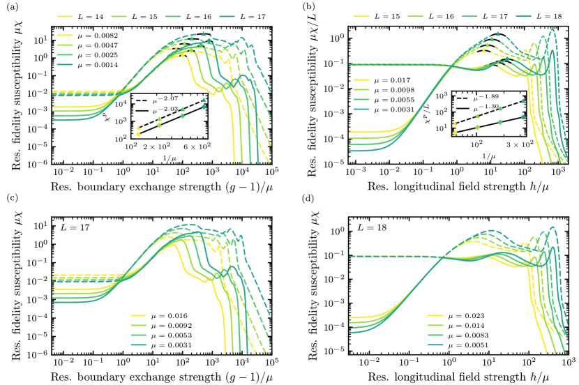
These scalings agree with numerical results (see Figs. 5b and  5d). Note that, at the critical value $h_{c}\sim\mu$ where $\chi_{g}=\chi_{h}$, the minimal and the maximal directions switch: in the regime where $h<h_{c}$, $\chi_{g}$ is smaller than $\chi_{h}$ and so $\varphi_{\text{min}}$ ($\varphi_{\text{max}}$) is aligned along the integrable (nonintegrable) direction, which is approximately parallel (perpendicular) to the line $h=0$. Similar analysis applies to the c-XXZ model such that at sufficiently large $L$ and small $\mu$ near the integrable line $g=1$, one expects

$$\chi_{g}\sim\frac{C}{\mu}\quad\text{and}\quad\chi_{h}\sim\frac{(g-1)^{2}}{\mu^{3}}\,.$$ (15)

Once again, these scalings agree with results in Figs. 5a and  5c but with slightly stronger finite-size effects, as the constant $C$ turns out to be rather small; the estimate in Eq. (13) is less accurate for smaller system sizes.

Figure 4: Relaxation dynamics of the Ising model. (a) shows the non-equal time correlation functions of $\partial_{\varphi}\mathcal{H}$ in the minimal (solid lines) and maximal (dashed lines) directions for $L=18$ at $g=1.5$ with $h=0.2,0.15,0.1$. Inset (i) shows the corresponding spectral function $\Phi_{\varphi}(\omega)$ for the same values of $h$. The dashed vertical line indicates the value of $\mu\approx 3.1\times 10^{-3}$ used while the dotted vertical line indicates the broadening $\Gamma=0.5\,\omega_{H}$, where $\omega_{H}$ is the typical level spacing, used to evaluate the spectral function (see Eqs. (17) and (18)). Inset (ii) shows $\varphi_{\text{min}}$ against $h$ near $h=0$. (b) shows $\Phi(\omega)$ in the $g$-direction (solid lines) and $h$-direction (dashed lines) for different values of $h$ with $L=18$. $\Gamma=0.5\,\omega_{H}$ is also used here. To reduce finite size effects, each $\Phi(\omega)$ is averaged over 3 different realizations of $g\in\{1.485,1.5,1.515\}$. Inset shows the same plot with frequency scaled by $h$ and the dotted line indicating perturbative result $(h/\omega)^{2}$.

Figure 5: Fidelity susceptibility vs. integrability breaking perturbation. In (a) and (c), we plot the rescaled fidelity susceptibility $\mu\chi$ against $(g-1)/\mu$ for the c-XXZ model near and above the integrable line $g=1$ at fixed $h=1.6$. Define $m=\sum_{i}\sigma_{i}^{z}$. For even (odd) $L$, we consider the $\expectationvalue{m}=0,\,\pm 2$ ($\expectationvalue{m}=\pm 1$) magnetization sectors. In (a), we vary $L$ and use $\mu=2L/\mathcal{D}_{s}$, where $\mathcal{D}_{s}=\binom{L}{\lfloor L/2\rfloor}$ and $\lfloor L/2\rfloor$ is the largest integer smaller than or equal to $L/2$. In (c), we fix $L=17$ and vary $\mu$ staying within the effective thermodynamic limit. In (b) and (d), we plot the rescaled fidelity susceptibility $\mu\chi/L$ ($\mu\chi$ for (d)) against $h/\mu$ near the integrable line $h=0$ with fixed $g=1.5$, where we use all $k\neq(0,\pi)$ quasi-momentum sectors. In (a), we vary $L$ and use $\mu=2.5\cdot L/\mathcal{D}_{s}$ with $\mathcal{D}_{s}=2^{L}/L$ while, in (d), we fix $L=18$ and vary $\mu$ within the effective thermodynamic limit. For (a)-(d), the solid (dashed) lines show fidelity susceptibility in the minimal (maximal) direction. Insets in (a) and (b) show the peaks of the minimal (maximal) $\chi$ against $1/\mu$ as diamonds (triangles) with fits given by the solid (dashed) lines.

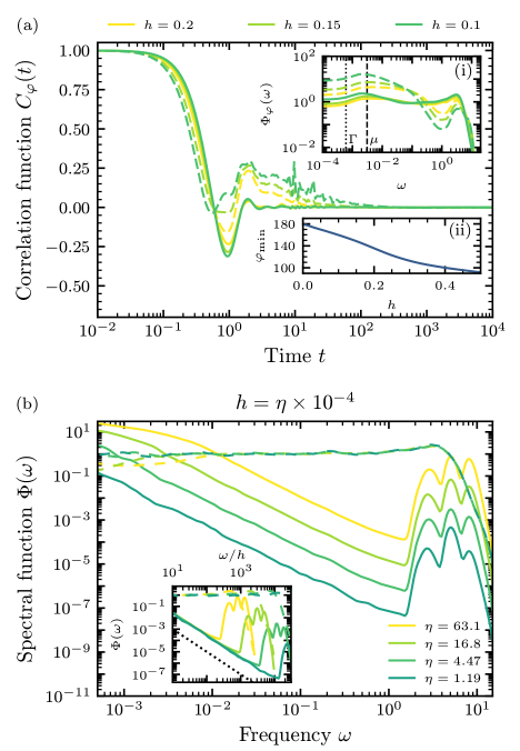
To understand the physical difference between maximal and minimal directions, let us examine the nonequal time correlation function $C_{\varphi}(t)$ and the corresponding spectral function $\Phi_{\varphi}(\omega)$. Here, we focus on the Ising model as it is more generic. For concreteness, we consider the Ising model at fixed $g=1.5$ and vary the small integrability breaking $h$. We show a similar analysis for the coupled XXZ model in Appendix C. The resulting $C_{\varphi}(t)$ computed at $L=18$ and for $h=0.2,0.15,0.1$ in both minimal ($C_{\text{min}}(t)$) and maximal ($C_{\text{max}}(t)$) directions are shown in Fig. 4a. We see that, for all values of $h$, $C_{\rm min}(t)$ relaxes much faster than $C_{\text{max}}(t)$. As we mentioned previously, the physical reason is due to the long prethermalization of observables conjugate to integrable directions. Perhaps surprisingly, we see no evidence of prethermalization in the direction $\varphi_{\rm min}$ for any value of $h$. This is in contrast to the c-XXZ model, where both minimal and maximal directions show prethermalization in the thermodynamic limit. The same conclusion can be reached by analyzing the spectral weight at low frequencies in the maximal direction (shown in inset (i) of Fig. 4a), which rapidly increases as $h\to 0$. Conversely, in the minimal direction, the spectral function only slightly depends on $h$. As $h$ approaches zero, we observe that $C_{\text{max}}\approx C_{g}$ decays at later times with increasingly noisy features marked by discrete many-body resonances due to finite level spacing [38, 16], while $C_{\text{min}}$ does not change much and so is not sensitive to these resonances.

Figure 6: Scaling of fidelity susceptibility. In (a) and (c), we plot the rescaled fidelity susceptibility $\mu^{2}\chi$ against $g-1$ for the c-XXZ model near the integrable line $g=1$ at fixed $h=1.6$. In (b) and (d), we plot the rescaled fidelity susceptibility $\mu\chi/L$ ($\mu\chi$ for (d)) against $h$ near the integrable line $h=0$ with fixed $g=1.5$. In (a) and (b), we vary $L$ and use $\mu=\alpha L/\mathcal{D}_{s}$ as defined in Fig. 5. In (c) and (d), we fix $L=17$ and $L=18$, respectively, and vary $\mu$ to be within the effective thermodynamic limit. For (a)-(d), we consider the symmetry sectors as described in Fig. 5, where the solid (dashed) lines show $\chi$ in the minimal (maximal) direction.

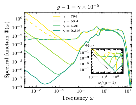
In Fig. 4b, we show the spectral function with very small integrability breaking perturbations, where the $\varphi_{\rm min}$ and $\varphi_{\rm max}$ directions approximately coincide with $g$ and $h$ directions, respectively. We see that the observable parallel to integrability $\partial_{g}\mathcal{H}$ has large overlaps with conserved operators and hence a large Drude weight at $\omega\to 0$. As the integrability breaking term is turned on, this Drude weight broadens, leading to a large spectral weight at low frequencies (see also Refs. [23, 15]). At large cutoff $\mu$, this low frequency spectral weight does not affect $\chi$ and so the minimal direction is approximately parallel to the $g$ direction. However, as $\mu$ becomes smaller, this low frequency tail dominates $\chi_{g}$ at decreasing values of $h$, leading to a sharper switch of $\varphi_{\rm min}$ from the direction orthogonal to integrability to the one parallel to it. In the inset of Fig. 4b, we show the collapse of the spectral function $\Phi_{g}(\omega)$ to the $(h/\omega)^{2}$ asymptote expected from perturbation theory.

Let us point out that in Ref. [15], contrary to this work, it was found that, even for a global integrability breaking perturbation, both integrability preserving and breaking directions showed similar scalings of the fidelity susceptibility with the system size for regions close to integrability. The reason is that the angle $\varphi_{\rm min}$ changes with the integrability breaking coupling. We found that the spectral function does not diverge as $\omega\to 0$ only along this special direction. For any other $\varphi\neq\varphi_{\rm min}$, the fidelity susceptibility is dominated by the divergent contribution coming from $\chi_{\rm max}$: $\chi_{\phi}\approx\sin^{2}(\varphi-\varphi_{\rm min})\chi_{\rm max}$, where we find that $\varphi_{\text{min}}$ scales linearly with respect to $h$ near $h=0$ as shown in inset (ii) of Fig. 4a.

V Scaling of Fidelity Susceptibility

Now we examine the scaling of the fidelity susceptibilities $\chi$ in minimal and maximal directions for both models near lines of integrability and thereby identify universal scaling of $\chi$ with integrability breaking perturbation. In Figs. 5a and 5b, we plot the rescaled $\mu\chi$’s in minimal and maximal directions against rescaled integrability breaking perturbations for the c-XXZ and Ising models, respectively. For the Ising model, we additionally divide $\chi$ by $L$ to account for the extensiveness of the perturbation $\partial_{\varphi}\mathcal{H}$. As found in Ref. [17], we find that $\mu=\alpha L/\mathcal{D}_{s}$ is a convenient scaling, where $\alpha$ is a number chosen to reduce finite size effects. These values of $\mu$ allow us to study the asymptotic limit $\mu\to 0$ as $L\to\infty$ while avoiding strong finite size effects due to discrete energy level spacing. For both plots, we achieve very good collapse, suggesting that in both directions near the integrable lines we have

$$\chi\sim\frac{1}{\mu}f_{1}\left(\frac{g-1}{\mu}\right),\quad\chi\sim\frac{L}{\mu}f_{2}\left(\frac{h}{\mu}\right),$$ (16)

for the c-XXZ and Ising models in the thermodynamic limit, respectively, where $f_{1}$ and $f_{2}$ are the scaling functions that depend on the direction. These scalings agree with Eqs. (15) and (14) but extend beyond the validity of perturbation theory, suggesting universality of the integrability to chaos transition similar to that in equilibrium continuous phase transitions. The insets in Figs. 5a and 5b show the scaling of the peaks of fidelity susceptibilities $\chi^{p}$. While we cannot extract scaling exponents accurately due to limited system sizes, the scaling of $\chi_{\text{min}}/L$ for the Ising model is consistent with $\chi^{p}\sim 1/\mu$ expected from a flat spectral function at small $\omega$, while the scalings of the other $\chi^{p}$’s are consistent with the maximally chaotic $1/\mu^{2}$ behavior [17]. Notably, in the Ising model, $\chi^{p}$ has a much stronger divergence with $\mu$ in the maximal direction, but, in the c-XXZ model, both minimal and maximal directions in thermodynamic limit saturate the upper bound of $\chi$. On the other hand, in Figs. 5c and 5d, we fix $L=17$ and $L=18$, respectively, and study the effective thermodynamic limit by varying $\mu$ within the range $1/\mathcal{D}_{s}\ll\mu\ll\mathcal{O}(1)$. For these values of $\mu$, $\chi$ is approximately system size independent up to weak power law corrections. Similar to Figs. 5a and 5b, we find very good collapse for $\mu\chi$ against $(g-1)/\mu$ and $\mu\chi$ against $h/\mu$ in Figs. 5c and 5d, respectively.

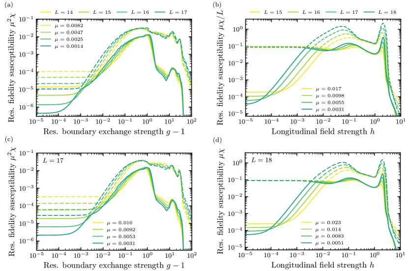
The difference between the c-XXZ and Ising models can be further highlighted by examining $\chi(L)$ with varying $L$ or $\chi(\mu)$ with fixed $L$ while varying $\mu$. In Figs. 6a and 6b, we plot $\mu^{2}\chi$ against $g-1$ and $\mu\chi/L$ against $h$ for the c-XXZ and Ising models, respectively, while varying $L$ with $\mu=\alpha L/\mathcal{D}_{s}$. On the other hand, in Figs. 6c and 6d, we plot $\mu^{2}\chi$ against $g-1$ at $L=17$ and $\mu\chi$ against $h$ at $L=18$ for the c-XXZ and Ising models, respectively, while varying $\mu$ within the range in which the effective thermodynamic limit for $\chi(\mu)$ is attainable. Focusing on integrability breaking perturbations of the order of one, we see collapses of $\mu^{2}\chi$ for the c-XXZ model and $\mu\chi$ (or $\mu\chi/L$) for the Ising model. As we discussed earlier, the latter scaling is consistent with a flat spectral function at small frequencies expected from ETH (see Ref. [5]). Hence, as in Ref. [15], we can conclude that the Ising model becomes ergodic in the thermodynamic limit for any value of $h$. On the contrary, for the c-XXZ model, the $\mu^{2}\chi$ collapse suggests that the system never becomes ergodic, i.e. the Thouless energy is zero, and so the low frequency tail of the spectral function extends all the way to the Heisenberg scale. We confirm this further by observing the lack of collapse of $\mu\chi$ for any value of $g-1$ and by analyzing the low frequency spectral functions (see Appendix C). Additionally, we see that the strength of the perturbation corresponding to the maximum value of $\chi$ rapidly falls to zero with decreasing $\mu$ for the Ising model (in agreement with Ref. [15]), while it barely changes with $\mu$ for the c-XXZ model. However, in the c-XXZ model, the range of perturbation strengths with $\mu^{2}\chi$ collapse expands towards lower strengths as $\mu$ diminishes. The reason for these behaviors is that as $\mu$ goes down and hence the time cutoff increases, the system can reach its asymptotic behavior for smaller perturbation strengths. From these observations we arrive at a very interesting conclusion: for the c-XXZ model with the boundary perturbation, chaos emerges for a tiny perturbation strength that quickly vanishes with the system size, which agrees with an earlier work in Ref. [17]. However, there is no indication that this model ever becomes truly ergodic, i.e. that it ever thermalizes. This behavior is more typical for zero-dimensional systems near the classical limit satisfying the KAM theorem [39].

VI Conclusions and Outlook

We found that integrable regions act as attractors of the adiabatic flows. Specifically, the flows in the directions that minimize the quantum geometric tensor lead towards integrable regions. We showed that the underlying reason for this behavior is due to faster relaxation of observables conjugate to these directions at small integrability breaking than for observables conjugate to directions parallel to integrability.

We analyzed two one-dimensional models representing the coupled XXZ chain and the Ising model with boundary and bulk integrability breaking perturbations, respectively. We numerically computed flow diagrams and identified distinct phases of flows that connect different or same areas of integrability. For both models, we found that the geometric tensor exhibits universal scaling behavior near integrable lines, suggesting a close analogy between emerging chaos and continuous phase transitions. As a side result, we found strong numerical indications that the Ising model becomes ergodic and so satisfies ETH in the thermodynamic limit for any value of the integrability breaking perturbation. Conversely, we found that the coupled XXZ chain for any nonzero perturbation is in a chaotic regime but never satisfies ETH: that is, it is never ergodic.

There is an interesting corollary of our results, which suggests that systems, where external couplings are treated as macroscopic dynamical degrees of freedom, can generically self tune themselves close to integrable regions during autonomous time evolutions. Thus, “integrability is attractive” not only in the mathematical sense but also as fixed points of time evolutions. This conclusion is in parallel to that of earlier works [40, 41], suggesting that, for systems close to the ground states, high symmetry or quantum critical points are natural attractors of dynamics. The physical reason of this dynamical attraction is that the divergent fidelity susceptibility comes with divergent dissipation and mass renormalization, leading to the freeze of time evolution along the directions with large $\chi$. Therefore, such dynamical systems would naturally evolve along the minimal directions.

Practically, our results pave the way to numerically finding nontrivial integrable or nearly integrable regimes either numerically by minimizing the norms of the adiabatic gauge potentials or experimentally by finding directions with fastest long-time relaxation. They also suggest that it is plausible to develop a full scaling theory of emergence of chaos similar to the theory of continuous phase transitions.

Appendix A Extrapolation of Flow Diagrams

Here, we provide details on our numerical extrapolation of the infinite temperature phase diagrams in the thermodynamic limit $L\to\infty$.

For the c-XXZ model, to visualize the growth of region A as defined in Fig. 3a, we examine the flow diagrams for system sizes $L=14,16,18$. As before, we consider the zero-magnetization sectors with $\mu=2L/\mathcal{D}_{s}$ and $\mathcal{D}_{s}=\binom{L}{L/2}$. We identify the outermost boundaries of the semicircular flows above $g=1$ and plot them for various $L$’s in Fig. 7a. As shown, the boundary grows outwards without any signs of slowing down as $L$ increases and so we expect that the region above the liine $g=1$ to be dominated by region A in the thermodynamic limit.

For the Ising model, we identify five regions A, B, B’, C, and D and then plot their boundaries for system sizes $L=16,18,20$ in Fig. 7b. Once again, we use all $k\neq(0,\pi)$ quasi-momentum sectors for $L=16,18$ and the $k=\pi/2$ quasi-momentum sector for $L=20$ with $\mu=2.5\cdot L/\mathcal{D}_{s}$ where $\mathcal{D}_{s}=2^{L}/L$. Here, region D (B’) denotes connectivity of the integrable point $I_{\infty}:\sqrt{h^{2}+g^{2}}\to\infty$ with itself (integrable line $g=0$) [see Fig. 2b for visualization of regions]. As shown, region A remains stable for $L\geq 18$ and region D tends to be pushed outward as $L$ increases. Further, the portion of region B’ that connects to the integrable point $I_{\infty}$ gets pushed rightwards as $L$ increases as shown by the extrapolated line. Then, in the thermodynamic limit, we expect region D to be nonexistent while regions B’ to become part of region B. Therefore, we only expect three regions (A, B, and C) to survive in the thermodynamic limit as shown in Fig. 3b.

Figure 7: Phase boundary lines of flows. (a) shows the growth of phase region that connects the integrable line $g=1$ with itself in the c-XXZ model for $L=14,16,18$ and (b) shows the phase regions A, B, B’, C, and D in the Ising model for $L=16,18,20$ (see text for more details). The black dotted lines in (b) are the linearly extrapolated phase boundary lines.

Appendix B Nonergodicity of the c-XXZ model

Figure 8: Fidelity susceptibility vs. boundary integrability breaking perturbation for the c-XXZ model. We plot the rescaled fidelity susceptibility $\mu\chi$ against $g-1$ for the c-XXZ model near the integrable line $g=1$ at fixed $h=1.6$.

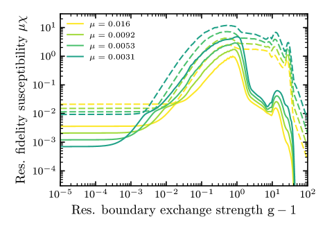
As shown in Figs. 6a and 6c of Sec. V, the fidelity susceptibility scales as $1/\mu^{2}$ in the c-XXZ model, which is a signature of maximally chaotic behavior. On the other hand, $\chi$ scales as $1/\mu$ in the Ising model, which is a necessary but not sufficient condition for ergodicity. Here, we observe that the c-XXZ model is nonergodic as $\chi$ does not scale as $1/\mu$. In Fig. 8, we plot $\mu\chi$ against $g-1$ at fixed $h=1.6$ for the c-XXZ model in the thermodynamic limit. We do not observe any signs of persistent collapse of $\mu\chi$ as $\mu\to 0$ and hence no sign of ergodicity for all values of $g-1>0$.

Appendix C Spectral analysis

As shown in Sec. V, the scaling of the fidelity susceptibility $\chi$ is quite different between the two models. Here, we systematically investigate these differences by computing the spectral functions $\Phi_{\varphi}(\omega)$ from Eq. (10), which can be calcuated using exact diagonalization

$$\Phi_{\varphi}(\omega)=\frac{1}{\mathcal{D}}\sum_{n}\sum_{m\neq n}\absolutevalue{\matrixelement{m}{\partial_{\varphi}\mathcal{H}}{n}}^{2}\delta(\omega-\omega_{mn})\,,$$ (17)

where $\delta(x)$ is replaced with the Gaussian

$$\delta(x)\to\frac{1}{\Gamma\sqrt{2\pi}}e^{-x^{2}/(2\Gamma^{2})}\,.$$ (18)

Here, $\Gamma$ is the broadening term that defines the width of the delta function. For subsequent computations (including those in the inset of Fig. 4), we use $\Gamma=\beta\,\omega_{\text{H}}>\omega_{\text{min}}$, where $\omega_{\text{H}}$ ($\omega_{\text{min}}$) is the typical (minimum) level spacing of the central $50\%$ of eigenstates and we choose $\beta\sim 0.1-0.5$ depending on the extent of the finite-size effects.

Figure 9: Spectral analysis of the Ising model. We plot the spectral function $\Phi(\omega)$ against frequency $\omega$ at $h=0.5$ in (a) and $h=1$ in (b). For each plot, the solid (dashed) lines show $\Phi(\omega)$ in the minimal (maximal) direction. Each $\Phi(\omega)$ is averaged over $3$ realizations of $g$ centered around $g=1.5$ with maximum deviation of $1\%$. The vertical dotted lines show the values of $\Gamma=0.5\,\omega_{\text{H}}$ used for different system sizes.

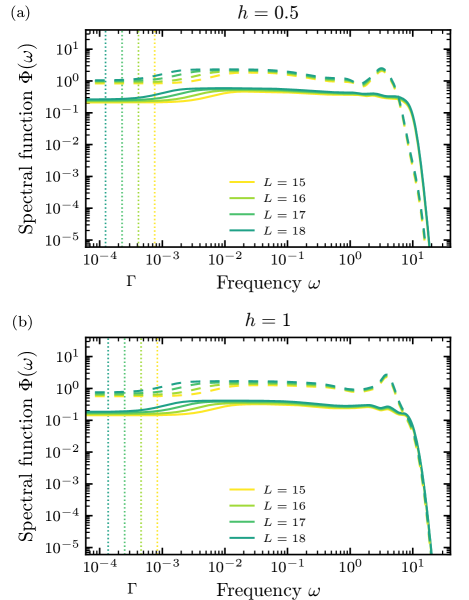
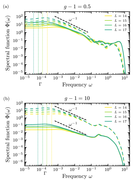
While we do not have a sufficient dynamical range to accurately extract the low-frequency asymptotes of the spectral functions, we can find their approximate power law scalings by fitting them to [23]

$$\Phi(\omega)=\frac{C}{\omega^{{\rm min}(1-1/z,0)}}\,,$$ (19)

where $C\equiv\Phi(\omega=1)$ and $z$ is the dynamical exponent. In an ergodic regime, we expect $z=2$ for regime $\omega>\omega_{\text{Th}}\sim 1/L^{2}$ while $z=0$ (exponential decay in time) when $\omega<\omega_{\text{Th}}$, where $\omega_{\text{Th}}$ is the Thouless frequency. The expected ETH scaling $\chi\sim 1/\mu$ corresponds to $z=0$ (more accurately $z<1$). In contrast, to observe $\chi\sim 1/\mu^{2}$ scaling saturating the maximum bound of fidelity susceptibility, we need $z\to\infty$ such that $\Phi(\omega)\sim 1/\omega$ . Next, we numerically verify these two expected behaviors of $\Phi(\omega)$ in the Ising and c-XXZ models, respectively.

In the Ising model, we observe signs of ergodicity, i.e. $\chi\sim 1/\mu$, for regions $h\sim 10^{-1}-10^{0}$ at fixed $g=1.5$ with the values of $\mu$’s considered in Sec. V. Hence, in Figs. 9a and 9b, we plot the spectral functions $\Phi(\omega)$ against the frequency $\omega$ at $h=0.5$ and $h=1$, respectively, for system sizes $L=15,16,17,18$. For each plot, we show $\Phi(\omega)$ in the integrable and nonintegrable directions. As expected, we find that $\Phi(\omega)$ is saturated for low frequencies as it is hard to see diffusive tail corresponding to $z=2$ for these system sizes and thus observe $\chi\sim 1/\mu$ scaling. For the c-XXZ model, we consider $g-1=0.5$ and $g-1=10$, where we observe $\mu^{2}\chi$ collapse in Figs. 6a and 6c, and plot the spectral functions for system sizes $L=14,15,16,17$ in Figs. 10a and 10b, respectively. We see that, at intermediate frequencies, $\Phi(\omega)\sim 1/\omega$ for both values of $g-1$, especially in the maximal directions, which lead to $\chi\sim 1/\mu^{2}$ scaling in the thermodynamic limit. The fit is better with some lower exponent $z$ in the minimal direction for $g-1=10$. However, the spectral function still shows tendency to diverge at $\omega\to 0$ as $L\to\infty$.

Finally, in Fig. 11, we plot the spectral function $\Phi(\omega)$ close to the integrable point $g=1$ at system size $L=17$ with $h=1.6$. As shown, the low frequency behaviors of $\Phi(\omega)$ in both minimal and maximal directions are quite similar as both directions show divergent spectral functions at $\omega\to 0$. This is in stark contrast to those shown in the Ising model (refer to $\Phi(\omega\to 0)$ in Fig. 4b), where, along the integrability breaking direction, the spectral function remains flat.

Figure 10: Spectral analysis of c-XXZ model at large integrability breaking. We plot the spectral function $\Phi(\omega)$ against frequency $\omega$ at $g-1=0.5$ in (a) and $g-1=10$ in (b). For each plot, the solid (dashed) lines show $\Phi(\omega)$ in the minimal (maximal) direction. Each $\Phi(\omega)$ is averaged over $3$ realizations of $h$ around $h=1.6$ with maximum deviation of $1\%$. The vertical dotted lines show the values of $\Gamma=0.1\,\omega_{\text{H}}$ used for different system size while the black dashed lines show the inverse frequency scaling of the spectral function: $\Phi(\omega)\sim 1/\omega$.

Figure 11: Spectral analysis of c-XXZ model at small integrability breaking. We plot the spectral function $\Phi(\omega)$ against frequency $\omega$ for several values of $g-1>0$. The solid (dashed) lines show $\Phi(\omega)$ in the $h$ ($g$ ) direction. Each $\Phi(\omega)$ is averaged over $3$ realizations of $h$ centered around $h=1.6$ with maximum deviation of $1\%$. $\Gamma=0.1\,\omega_{\text{H}}$ is used. Inset shows $\Phi(\omega)$ against $\omega/(g-1)$ while the dotted line indicates the $(\omega/(g-1))^{-2}$ asymptote.

References

- Berry [1989] M. Berry, Physica Scripta 40, 335 (1989).
- Haake [1991] F. Haake, Quantum signatures of chaos, in Quantum Coherence in Mesoscopic Systems, edited by B. Kramer (Springer US, Boston, MA, 1991) pp. 583–595.
- Stöckmann [1999] H.-J. Stöckmann, Quantum Chaos: An Introduction (Cambridge University Press, 1999).
- Borgonovi et al. [2016] F. Borgonovi, F. M. Izrailev, L. F. Santos, and V. G. Zelevinsky, Phys. Rep. 626, 1 (2016).
- D’Alessio et al. [2016] L. D’Alessio, Y. Kafri, A. Polkovnikov, and M. Rigol, Advances in Physics 65, 239 (2016).
- Brody et al. [1981] T. A. Brody, J. Flores, J. B. French, P. A. Mello, A. Pandey, and S. S. M. Wong, Rev. Mod. Phys. 53, 385 (1981).
- Guhr et al. [1998] T. Guhr, A. Müller–Groeling, and H. A. Weidenmüller, Physics Reports 299, 189 (1998).
- Srednicki [1999] M. Srednicki, Journal of Physics A: Mathematical and General 32, 1163 (1999).
- Deutsch [2018] J. M. Deutsch, Reports on Progress in Physics 81, 082001 (2018).
- Berry and Tabor [1977] M. V. Berry and M. Tabor, Proceedings of the Royal Society of London Series A 356, 375 (1977).
- Rigol et al. [2007] M. Rigol, V. Dunjko, V. Yurovsky, and M. Olshanii, Phys. Rev. Lett. 98, 050405 (2007).
- Berges et al. [2004] J. Berges, S. Borsányi, and C. Wetterich, Phys. Rev. Lett. 93, 142002 (2004).
- Moeckel and Kehrein [2008] M. Moeckel and S. Kehrein, Phys. Rev. Lett. 100, 175702 (2008).
- Durnin et al. [2021] J. Durnin, M. J. Bhaseen, and B. Doyon, Phys. Rev. Lett. 127, 130601 (2021).
- LeBlond et al. [2021] T. LeBlond, D. Sels, A. Polkovnikov, and M. Rigol, Phys. Rev. B 104, L201117 (2021).
- Bulchandani et al. [2022] V. B. Bulchandani, D. A. Huse, and S. Gopalakrishnan, Phys. Rev. B 105, 214308 (2022).
- Pandey et al. [2020] M. Pandey, P. W. Claeys, D. K. Campbell, A. Polkovnikov, and D. Sels, Phys. Rev. X 10, 041017 (2020).
- Surace and Motrunich [2023] F. M. Surace and O. Motrunich, arXiv preprint arXiv:2302.12804 10.48550/arXiv.2302.12804 (2023).
- Orlov et al. [2023] P. Orlov, A. Tiutiakina, R. Sharipov, E. Petrova, V. Gritsev, and D. V. Kurlov, Phys. Rev. B 107, 184312 (2023).
- Zanardi and Paunković [2006] P. Zanardi and N. Paunković, Phys. Rev. E 74, 031123 (2006).
- Campos Venuti and Zanardi [2007] L. Campos Venuti and P. Zanardi, Phys. Rev. Lett. 99, 095701 (2007).
- Kolodrubetz et al. [2013] M. Kolodrubetz, V. Gritsev, and A. Polkovnikov, Phys. Rev. B 88, 064304 (2013).
- Sels and Polkovnikov [2021] D. Sels and A. Polkovnikov, Phys. Rev. E 104, 054105 (2021).
- Zhang et al. [2022] Y. Zhang, L. Vidmar, and M. Rigol, Phys. Rev. E 106, 014132 (2022).
- Provost and Vallee [1980] J. Provost and G. Vallee, Commun. Math. Phys. 76, 289 (1980).
- Kolodrubetz et al. [2017] M. Kolodrubetz, D. Sels, P. Mehta, and A. Polkovnikov, Physics Reports 697, 1 (2017).
- Helstrom [1976] C. W. Helstrom, Quantum Detection and Estimation Theory, ISSN (Elsevier Science, 1976).
- Funo et al. [2017] K. Funo, J.-N. Zhang, C. Chatou, K. Kim, M. Ueda, and A. del Campo, Phys. Rev. Lett. 118, 100602 (2017).
- Bukov et al. [2019] M. Bukov, D. Sels, and A. Polkovnikov, Phys. Rev. X 9, 011034 (2019).
- Peotta et al. [2023] S. Peotta, K.-E. Huhtinen, and P. Törmä, Quantum geometry in superfluidity and superconductivity (2023), arXiv:2308.08248 [cond-mat.quant-gas] .
- Sugiura et al. [2021] S. Sugiura, P. W. Claeys, A. Dymarsky, and A. Polkovnikov, Phys. Rev. Res. 3, 013102 (2021).
- Note [1] In this paper, we are only interested in its real part also referred to as Fubini-Study metric tensor.
- Note [2] For all subsequent calculations, we always consider only the central of the eigenstates.
- Note [3] is approximately the level spacing of the system.
- Alcaraz et al. [1987] F. C. Alcaraz, M. N. Barber, M. T. Batchelor, R. Baxter, and G. Quispel, Journal of Physics A: mathematical and general 20, 6397 (1987).
- Gubin and F. Santos [2012] A. Gubin and L. F. Santos, Am. J. Phys 80, 246 (2012).
- Kim et al. [2014] H. Kim, T. N. Ikeda, and D. A. Huse, Phys. Rev. E 90, 052105 (2014).
- Bukov et al. [2016] M. Bukov, M. Heyl, D. A. Huse, and A. Polkovnikov, Phys. Rev. B 93, 155132 (2016).
- Lim et al. [shed] C. Lim, K. Matirko, A. Polkovnikov, and M. Flynn, (unpublished).
- Kofman et al. [2004] L. Kofman, A. Linde, X. Liu, A. Maloney, L. McAllister, and E. Silverstein, Journal of High Energy Physics 2004, 030 (2004).
- Kolodrubetz et al. [2015] M. Kolodrubetz, E. Katz, and A. Polkovnikov, Phys. Rev. B 91, 054306 (2015).
- Weinberg and Bukov [2017] P. Weinberg and M. Bukov, SciPost Phys. 2, 003 (2017).
- Weinberg and Bukov [2019] P. Weinberg and M. Bukov, SciPost Phys. 7, 020 (2019).
- Note [4] Note that scaling can be also explained if decays faster than but then there must exist a low frequency cutoff below which the spectral function must saturate [15].