Depleting states dictate the ideal glass and physics of glass transition

Abstract

Understanding the properties of supercooled fluids in equilibrium, even below the calorimetric glass transition $T_{g}$, is an elusive challenge. This is even more true for the properties of the ideal glass, defined as the minimum of the potential energy landscape (PEL) in the non-crystalline regime. Although its existence is a mathematical necessity due to the finite range of energies, its properties, and physical relevance are still undecided. Here we combine the million-fold acceleration of Swap Monte Carlo with PEL analysis to study a non-network 2D model glass former in equilibrium for a wide range of system sizes and temperatures. We observe the transition from fragile to strong behavior and provide a generic perspective to such observations in many experimental non-network glass formers, or the saturation of structural disorder upon cooling. Furthermore, we can identify a particular system size that shows quantitative agreement with the macroscopic limit, while allowing a complete characterization of the potential energy landscape (PEL) down to its global minimum. This implies the availability of configurational entropy down to the zero temperature limit without the detour via liquid entropy, thereby quantifying the putative entropy crisis. Through appropriate system size analysis, we can identify a low-energy depletion regime, including the ideal glass, and reveal its physical relevance for equilibrium properties over a wide temperature range, including below $T_{g}$.

Introduction— Glass, a disordered material, has remained ubiquitous in human civilization for millennia. Furthermore, the intriguing and elusive problem of the nature of glasses, emerging upon cooling a supercooled liquid, persists as an unsolved and notorious enigma in the realm of condensed matter physics Anderson (1995). With its broad range of applicability, glass finds relevance across a spectrum of materials, from polymers and alloys to colloids, thereby marking its significance in a diverse array of applications Debenedetti and Stillinger (2001). The equilibrium window of supercooling, metastability below melting, ranges from 100ps to 100s of structural relaxation in the laboratory, marking the onset ($T_{onset}$), and experimental glass transition temperature ($T_{g}$), respectively Schmidtke et al. (2012). Glass-forming liquids fall into two classes based on their temperature dependence of dynamical behavior: “strong” liquids with exponential dependence on inverse temperature (known as the Arrhenius relation) and “fragile” liquids with a super-Arrhenius (SA) behavior, exhibiting a stronger-than-exponential dependence Angell (1991a). Network formers such as silica and water display both types of dynamics, separated by a characteristic Fragile to Strong Crossover (FSC) in the supercooled regime  Saika-Voivod et al. (2001); Saksaengwijit et al. (2004).

Thermodynamics-wise, a relation between dynamics and entropy has been formulated in well-known approaches such as Adam-Gibbs Adam and Gibbs (1965) or the Random first-order transition (RFOT) theory  Lubchenko and Wolynes (2007); Kirkpatrick et al. (1989). For network formers, the emergence of the FSC indeed goes along with an inflection of the entropy Saika-Voivod et al. (2001). The distinct characteristics intrinsic to the system present a formidable obstacle in constructing a comprehensive theoretical framework to decipher the nature of glass.

The potential energy landscape (PEL), as a general approach, one studies the distribution of the inherent structures (IS), i.e., local energy minima (denoted IS-density), and their topology. This information helps to elucidate the underlying nature of thermodynamic and dynamical properties Goldstein (1969); Angell (1991b); Sastry (2001); Sciortino (2005); La Nave et al. (2006); Heuer (2008); Baity-Jesi et al. (2021). If the complete density of states, including its ground state, were known, important thermodynamic properties such as entropy or specific heat could be directly deduced for all temperatures. Thus, the PEL approach has the potential to provide answers to fundamental questions of glass physics, including the nature of fragility, the ideal glass corresponding to the ground state of the IS, and the nature of approaching the zero-temperature entropy, which so far remains unanswered due to the astronomical time scales of relaxation Berthier and Biroli (2011).

A PEL study requires the use of relatively small system sizes because for large systems, the information content is reduced due to the presence of many uncorrelated subsystems Doliwa and Heuer (2003); Heuer (2008). Thus, one looks for system sizes $N$ that are as small as possible, while ensuring minimal finite-size effects for thermodynamic, structural, and dynamical observables. Denoting $N_{c}$ as the corresponding system size, reasonable choices were $N_{c}=65$ for binary 3D Lennard-JonesKob and Andersen (1994); Doliwa and Heuer (2003), $N_{c}=99$ for 3D BKS-silica  Saksaengwijit et al. (2004), and $N_{c}=80$ for 2D silica Roy and Heuer (2022). For the network formers, it was even possible to extract the complete IS-density for $N=N_{c}$, displaying a Gaussian energy dependence with a sharp decay at low energies Saksaengwijit et al. (2004); Roy and Heuer (2022). An alternative structural approach to silica can also be found Yu et al. (2022). The emergence of this cutoff has been related to the presence of well-defined low-energy states void of defects such as dangling bonds Saksaengwijit et al. (2004), and a subtle structural change Yu et al. (2022); Roy and Heuer (2022). The FSC emerged as a consequence of that cutoff. Beyond the special case of network formers, the complete IS-density is unknown for system sizes around $N_{c}$ due to the necessity of exponentially demanding numerical burden at low energies.

Here we study a 2D non-network glass former via the swap Monte Carlo technique Ninarello et al. (2017). With the removal of previous sampling limitations, we generate a large ensemble of equilibrium configurations for system sizes $N\in[33,1056]$ and for the temperature range $T\gtrsim T_{g}/2$, i.e., even exceeding the experimentally relevant regime $T>T_{g}$, while no crystallization was observed. This allows the reconstruction of the IS-density relevant for the range $T\gtrsim T_{g}/2$. Importantly, after identifying an appropriate system size $N_{c}$, we can show that for $N\leq N_{c}$ even the complete IS-density, including the bottom state, can be determined. Consequently, for that range of system sizes, thermodynamic and structural properties can be completely described for all temperatures $T>0$ (neglecting quantum-mechanical effects), and the configurational entropy can be obtained without starting from the liquid entropy and using techniques like thermodynamic integration. For $N>N_{c}$, it will turn out that this physical insight is at least relevant for $T\gtrsim T_{g}/2$, i.e., for all experimentally relevant and exceeding supercooling. Furthermore, also an FSC can be identified at low $T$, providing unprecedented information about the presence and origin of the FSC in non-network formers. Furthermore, a comparison with corresponding experiments and conclusions about Kauzmann’s paradox is possible.

Specifically, we analyze a discrete-polydisperse mixture of purely repulsive spheres with $10$ particle types in two dimensions. The composition is kept strictly the same for all system sizes, ensuring consistency in the study; see the Methods section for details Ninarello et al. (2017); Parmar et al. (2020). Equilibrated configurations are generated for a wide range of system sizes $N\in\{33,66,132,264,528,1056\}$ and temperatures $T\in[0.0263,0.5]$, where the calorimetric glass transition temperature is $T_{g}=0.0555$, associated to time scales of 100 s. The lowest equilibrated sample from the swap moves corresponds to astronomical time scales of $10^{21}$s. The well-equilibrated independent samples from the swap MC were used as the initial sample for the NVT-MD simulations with LAMMPS Plimpton (1995). The dynamics of the system explored for $T\in[0.069,0.5]$, spanning 7(10) decades of diffusion(relaxation) below the onset temperature($T_{onset}=0.25$). The simulation at the lowest T is pushed to $t=6\cdot 10^{8}$ MD time, roughly corresponding to the millisecond time scale. In what follows, $e_{IS}=E_{IS}/N$ is the IS energy per particle.

Figure 1: Finite-size effects and dynamics. a The energy fluctuation per particle for two different temperatures. It decreases proportionally to $N^{-1/2}$. b The finite-size effect of the average IS energy relative to the fluctuations, for the same two temperatures. Included is an empirical $1/N$ asymptotic behavior (dashed line). c The inverse diffusion constant $1/D$ (scaled with $D_{o}$, diffusion at the onset temperature) covers 7 decades of glassy dynamics. It reveals the crossover from fragile to strong behavior at low T($\lesssim 0.1$). The inset presents the low and high-T activation energy ratio for all system sizes.

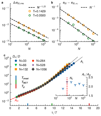
Quantifying finite-size effects— We start by evaluating the size dependence of the standard deviation and the average energy of the IS-density at two different temperatures. In the large system size limit, one expects that a system of size $2N$ can be considered as an independent superposition of two systems with size $N$. This superposition hypothesis implies that the standard deviation of the energy distribution (per particle) scales like $N^{-1/2}$ as indeed observed for all N, see Fig. 1(a). Generally, the energy $E_{N}$ will deviate by a constant $c/2$ from the large-size limit $Ne_{\infty}$. Then the relation $E_{2N}=2E_{N}$, resulting from the superposition hypothesis, yields $e_{2N}=E_{N}/N=e_{\infty}+c/(2N)$, i.e. $e_{N}-e_{\infty}\propto 1/N$. Also, this relation holds very well (Fig. 1b) for the whole range of $N$-values and for both temperatures. Thus no deviations from the superposition hypothesis are visible for $N\geq 33$.

The diffusion constant is an appropriate observable for the identification of finite-size effects of the transport behavior Rehwald et al. (2010). The results are shown in fig. 1c. The emergence of an FSC at low temperatures ($T\lesssim 0.1$) can be observed for all system sizes. The ratio of the low-T ($A_{L}$) and high-T ($A_{H}$) activation energies are displayed in fig. 1c( inset). Thus, a system as small as $N=33$ reflects the dynamics in the thermodynamic limit on a semi-quantitative level, whereas for $N=66$, even a nearly quantitative agreement can be observed. Detailed analysis shows, also for structural relaxation (SI (VI)), that the low-T dynamics is incompatible with alternative standard descriptions for supercooled liquids. The resulting choice $N_{c}=66$ is also well supported by the weak $N$-dependence of the participation ratio for $N\geq N_{c}$, quantifying the number of mobile particles in relaxation events during an IS-IS transition (see SI (V)) Vogel et al. (2004)).

Figure 2: From depletion to the bottom of the PEL. The per-particle potential energy of IS with system sizes (a) N=33 and (b) N=66, respectively. The color bar for each temperature represents the equilibrium probability distribution. The deviation from the observed Gaussian behavior in the initial supercooled regime is stressed with the dashed line fitted for the temperature range $T\in[0.1429,0.25]$. The horizontal lines represent the lowest energy of IS for both system sizes. c &d The Boltzmann energy distributions, for $N\in[66,264]$ compared with the distribution of subsystems of size $N/2$, suggest the subsystem does satisfactorily characterize the larger system. Since the $N=66$ system accesses much lower energies than the $N=33$ system, deviations for this comparison have to occur in the low-energy region (as in c).

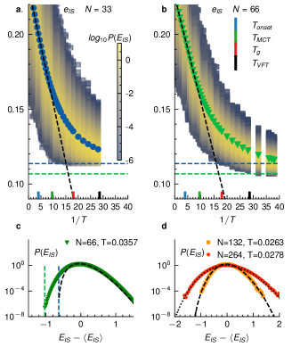
The energy distribution— A meticulous analysis of the energy distribution across various system sizes, temperatures, and energy levels yields further insights and understanding. First, we report the Boltzmann distribution $P(E_{IS},T)$ of IS energies, determined at different temperatures, as well as its first moment for $N=33$ and $N=66$, see Fig. 2(a&b). For $T>0.1$ we observe a linear behavior of the average IS energy with respect to the inverse temperature. This is known to reflect a Gaussian distribution of IS Heuer and Büchner (2000). For all systems sizes, around $T\lesssim 0.1$, the slope starts to decrease for decreasing temperature (also for $N>66$, see SI (IV)). This is caused by the depletion of low-energy states, as seen from the emerging asymmetric distribution. Importantly, the occurrence of the FSC manifests at exactly the temperature where the non-Gaussian regime of the PEL becomes relevant, independent of system size. This suggests a very strong relationship between both observations.

At still significantly lower temperatures, the bottom of the landscape is found, namely for $N=33$ at $T\approx 0.06$ (close to the calorimetric $T_{g}$), and for $N=66$ at much lower temperatures (around $T_{g}/2$). Its identification required these extensive simulations. The claim that the bottom of the PEL is indeed found is further supported by statistical arguments (see SI (VII) and SI (VIII)), stating that for $N=66$, all the 16 lowest energies are found for both the lowest two temperatures. The IS at the bottom has lower energy for $N=66$. Most importantly, for the first time, the whole IS-distribution is now accessible for system size $N_{c}$.

One might conclude that the different temperatures, required for the identification of the bottom of the PEL, is related to the different energies (per particle) at the bottom. However, as argued in SI (VI), this effect would also be present if the superposition hypothesis is strictly valid, implying identical bottom energies. This is also the reason why it is not possible to find the bottom of the PEL for $N=132$ (estimated required temperature: 0.02).

The Boltzmann distributions $P(E_{IS},T)$ can be further explored to check the superposition hypothesis, see Fig. 2(c&d). Here we show the actual distributions at different sizes $N$ and their prediction via the superposition hypothesis, based on the distribution at size $N/2$ (see Methods). The temperatures are chosen far below $T_{g}$. For the transition from $N=33$ to $N=66$, we see a very good agreement for higher energies, whereas deviations are visible on the low-energy side. This was expected due to the shifted bottom of the PEL, as observed in Fig. 2(a&b). Remarkably, we see a perfect superposition for the transitions $N=66\rightarrow N=132$ and $N=132\rightarrow N=264$ for the whole energy range, supporting the choice $N_{c}=66$ again.

Figure 3: From the energy distribution to the configurational entropy. a The energy distribution of IS for various system sizes across the ultra-stable limit. The dashed-colored lines show a Gaussian fit from the higher energy supercooled regime, revealing faster depletion of states than predicted for a pure Gaussian. The dashed-black line depicts the distribution constructed from the respective half-sized subsystem. The vertical-colored lines represent the lowest energy for IS for N=33 and 66. b For $N=33,66$, the configurational entropy is calculated from the complete IS energy distribution, including the information of the basin’s volumes from the Hessian (see SI (IX)). For $N\geq 132$, the entropy curves are shifted to agree with N=66 at $T_{MCT}=0.105$. The inset compares the ‘shifted’ entropy for $N=33$ to $N=66$ at $T_{MCT}$ and its range of (nearly) perfect agreement. The vertical dashed line represents $T_{g}/2$.

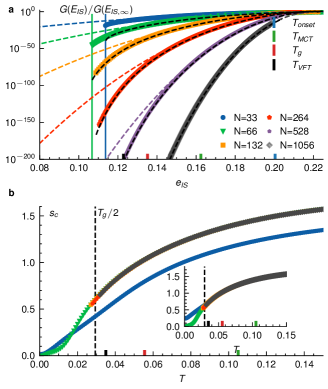
A more profound picture of the PEL can be obtained from knowledge of the IS-density, written as $G(E_{IS})$. It is defined such that the equilibrium probability is given by $P(E_{IS},T)\propto G(E_{IS})\exp(-\beta E_{IS})$ with $\beta=1/{k_{B}T}$. Thus, $G(E_{IS})$ can be obtained by reweighting Saksaengwijit et al. (2004). Strictly speaking, the IS-density additionally contains the information about the effective volume of the basin, i.e., $G(E_{IS})=\sum_{i}Y_{i}\delta(E-E_{i,IS})$ where the factor $Y_{i}$ expresses the volume contribution. Thus, one should rather speak of a volume-weighted IS-density. In harmonic approximation, $Y_{i}$ is related to its curvature at the minimum and is estimated from the eigenvalues of the Hessian Sciortino (2005) (for more details and the negligible impact of additional anharmonic corrections, see SI (IX)). In Fig. 3(a) $G(E_{IS})$ is displayed in a normalized continuous representation. One can explicitly observe the depletion of IS at low energies, giving rise to a transition from Gaussian to non-Gaussian density, as already reflected in Fig. 2. Consistent with Fig. 2(c&d), the superposition hypothesis is also valid for $G(E_{IS})$ for the whole range of energies. The only deviations are seen for the transition $N=33\rightarrow N=66$ close to the bottom of the PEL. It cannot be excluded that the superposition hypothesis is also violated for larger $N$ in the range of very low energies. However, these differences would, if at all, only be visible for $T<T_{g}/2$, and thus not relevant for experiments.

Note that the non-Gaussian energy regime becomes much more dominant for large system sizes simply because of the superposition effect, i.e., the underlying convolution of the energy distributions. In contrast, for $N=33$, the non-Gaussian regime is quite small. Note that even the $N=33$ system can be viewed as a superposition of even smaller entities, as evidenced by much smaller values of the participation ratio (see SI (V)). Thus, the non-Gaussian regime even for the $N=33$ system can be seen as a consequence of the finite energy range of the PEL. We have reported that the onset temperature of the FSC appears when the depletion of low-energy states and thus non-Gaussian effects become relevant. Based on our observations, this suggests that the FSC is influenced by the presence of the bottom of the PEL of small-scale units. As already discussed exclusively for network formers, the presence of a low-energy bottom generally leads to low-T Arrhenius behavior Saksaengwijit et al. (2004).

Of utmost relevance for the discussion of the properties of glass-forming systems is the configurational entropy, defined via the Shannon description as $S_{c}(T)=-\sum_{i}P(E_{i,IS},T)\ln P(E_{i,IS},T)$ where the sum is over all the IS. Since $P(E_{i,IS},T)\propto Y_{i}\exp(-\beta E_{i,IS})$, the configurational entropy can be rewritten as (see SI (IX)) $S_{c}=-\langle logY_{i}\rangle+\beta\langle E_{i,IS}\rangle+\ln(\sum_{i}Y_{i}\exp(-\beta E_{i,IS}))$. Whereas the first two terms are thermodynamic averages, the last term requires knowledge about the absolute number of IS, which is available for $N=33$ and $N=N_{c}=66$. Thus, the complete knowledge of the PEL for both systems unveils a unique prospect for evaluating the configurational entropy for all temperature ranges without resorting to the liquid entropy. For larger $N$, where the ground state is unknown, the entropy can be directly obtained apart from a temperature-independent shift factor and can be calculated for the temperature range, for which equilibrium simulations are available.

Fig. 3b shows the configurational entropy for various system sizes. For $N=N_{c}=66$ its temperature dependence, involving a transition from positive to negative curvature at low but finite temperature (see also SI (IX)), reflects the low-energy state depletion, including the cutoff. For the present model glass, it stems a unique footing to quantify Kauzmann’s picture of entropy crisis Kauzmann (1948) and provides a direct view of the thermodynamic behavior Angell (2008) such as the nature of the strong decrease of entropy at low temperatures Berthier et al. (2019) due to the direct relation to individual states.

One might have expected that the entropy for $N=33$ only differs for low temperatures because of the lack of low-energy states as seen, e.g., in Fig.3a. Indeed, for $T>0.04$, the shape of the entropy curve is identical. However, the absolute value differs significantly as seen in Fig. 3b, i.e., the number of IS for all energies is by a factor $exp[(s_{c}(N=66)-s_{c}(N=33))\cdot 66]\approx 10^{7}$ higher for $N=66$ as expected from the factorization properties. This reveals a surprising entropy variation, although other thermodynamic properties (i.e., average energy) or the diffusivity are qualitatively similar for $N=33$ and $N=66$ in the whole temperature range. A simple suggestion for this thermodynamic finite-size effect of the absolute number of states is provided in the SI (IX), suggesting a dominant $\ln(N)/N$-dependence of the configurational entropy.

Figure 4: Structural features across the PEL. a & b The lowest energy sample was explored during a wide range of temperatures. For N=33(66), the lowest energy configuration is shown for T=0.0385(0.0270) and T=0.0357(0.0263) with filled and dashed styles, respectively. The color scheme represents the diameter of the particle. c The disorder depicts a similar temperature dependence as the energy. d The parametric plot between the structural disorder and the potential energy provides a comprehensive approach to studying the disorder. e The mean diameter for the neighbors of the particle $i$ with diameter $\sigma_{i}\geq 1.4$ for a range of temperatures across $T_{g}$. The distinct nature of N=33 suggests that the variety of possible configurations is not large enough for the smallest system.

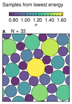
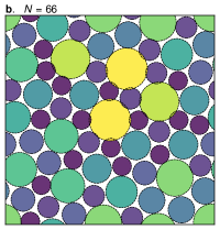
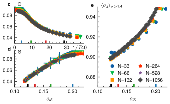
Lowest state and structure— To quantitatively characterize the low-energy state, Fig. 4a&b presents the ground states observed at various temperatures for $N=33$ and $N=66$, respectively. Evidently, the packaging suggests a strong anti-correlation between larger and smaller particles.

Inspired by the network-forming liquids, the structural features of the IS are expected to characterize the system’s disorder, depending on their energy Roy and Heuer (2019). One can quantify the disorder ($\Theta$) as the deviation from steric arrangements with the Voronoi neighbors (see methods) Tong and Tanaka (2018). Upon cooling, already above $T_{g}$ one can see the approach towards a constant disorder, see Fig. 4c. The temperature dependence is very similar to that of the energy (Fig. 2). Indeed, this is a direct consequence of the linear relationship between disorder and energy, see Fig. 4d, complemented by the presence of the low-energy cutoff. Since structural features are also accessible experimentally, a signature of the bottom of the PEL might thus be observable. This structural feature does not display any finite-size effects, even not for $N=33$.

Another structural property is a possible correlation of the diameters of adjacent particles. For this purpose, we report the mean diameter of the Voronoi neighbors for particles with $\sigma\geq 1.4$ for system sizes between $N=33$ and $N=1056$, see Fig.4e. For lower energies, a stronger anti-correlation between adjacent diameters is observed. The deviations for $N=33$ in the low-energy limit possibly reflect the smaller number of possible arrangements. The stronger anti-correlations enable a more efficient packing of the particles and thus the accessibility of lower energies. The analog of this statistical feature is the disappearance of well-defined defects in the case of network formers when reaching the low-energy limit. Such an order parameter does not exist for the present non-network system, yielding a contrasting perspective on both types of glass formers.

Experimental system— The study by Hecksher et al.  Hecksher et al. (2008) suggests a possibility of VFT-like divergence not being a complete description of the glassy dynamics, which is further corroborated by Mallamace et al.  Mallamace et al. (2010) for a variety of experimental systems suggesting strong behavior in the low-T limit in supercooled liquids. In the context of FSC, we analyze a range of fragile experimental glassy systems and observe that the low-T dynamics(below $T_{onset}$) possess 4 to 12 decades to be described with the Arrhenius relation (see SI (XI)). The exact reasoning behind such crossover is not clearly understood. Whereas, e.g., Mallamace et al.  Mallamace et al. (2010) proposed dynamics heterogeneity’s role with a crossover around a viscosity $10^{3}$ Poise, in other approaches the crossover is predicted either in the vicinity of $T_{MCT}$ Casalini et al. (2003a, b), or via excluded volume based theory close to $T_{g}$ Rah (2007). The state-of-the-art measurements for the 20 million-old amber Zhao et al. (2013), metallic glass Zhang et al. (2010), and viscosities beyond laboratory glass transition Pogna et al. (2015); Jadhao and Robbins (2017) highlight the lack of understanding of the temperature dependence of dynamics. Based on the arguments for such a wide range of systems, our study proposes a general framework to comprehend the emergence of Arrhenius behavior at low-T within the context of the PEL.

Discussion— The study accentuates a central issue regarding the relaxation dynamics of supercooled liquids near the experimental glass transition and beyond. Combining the idea of the study of relatively small systems with the swap simulation, we can investigate the energy landscape for an equilibrium relaxation time span of astronomical scale, thus achieving a view of the complete energy landscape. The non-Gaussian nature of PEL appears to be a general characteristic of glasses and not a special feature of network formers. Consequently, the crossover to Arrhenius behavior can be seen as a general glassy feature, avoiding any finite-T divergence. It also contextualizes the recent observations of low-T Arrhenius behavior, reported in other independent simulation studies Berthier and Ediger (2020); Guiselin et al. (2022); Das and Sastry (2022). The results presented in this work provide a broad perspective on glass physics, extending beyond experimental time scales.

The novel finding of crossover for the PEL and dynamics may represent a mechanism that can follow Kauzmann’s scenario for the glassy state, providing valuable insights into the fundamental nature of glass. The corresponding depletion of low-energy states is mainly a consequence of the energy cutoff, seen for the smallest studied system. Additionally, this supports the idea that systems cannot be aged without crystallizing to arbitrarily deep energies; such observation could be crucial for modeling energy landscapes and mesoscale modeling of glass. Finally, our investigation paves the way for new studies for experimental and model glass formers within the context of PEL and understanding the dynamics around and below $T_{g}$ and possibly also about the impact of the dimensionality on the low-energy and thus low-temperature properties.

Glass forming in-silico model— We study a discrete-polydisperse mixture of $N$ purely repulsive particles, consisting of $M$ species of equal mass $m$, pairwise interacting via power-law potential. The purely repulsive interaction potential for particles $i$ and $j$, at the distance $r_{ij}$ is defined as

$$e(r_{ij})=\epsilon\left(\frac{\sigma_{ij}}{r_{ij}}\right)^{12}+\sum_{k=\{0,2\}}c_{2k}\left(\frac{r_{ij}}{\sigma_{ij}}\right)^{2k},$$ (1)

with interaction range $r_{ij}/\sigma_{ij}(=r_{c,ij})\leq 1.25$. The fourth-order polynomial ensures that the potential, force, and second-order derivatives are continuous at the cutoff. We use $\epsilon$ as the unit of energy and temperature and average particle diameter $\left<\sigma\right>$ as the unit of length. The molecular dynamics time is measured in reduced units of $\sqrt{m\left<\sigma\right>^{2}/\epsilon}$, while the Monte Carlo time is reported as the MC steps performed. We study the system sizes ranging from N=33 to 1056, consists of $M=10$ species, following the diameter-distribution $P(\sigma)\propto\sigma^{-3}$  Ninarello et al. (2017), with $\sigma\in[0.73,1.62]$. Such a strategy for modeling allows for rigorous comparison of various system sizes while keeping the size-disorder identical Parmar et al. (2020)(see SI(I)). In addition to polydispersity, to ensure good glass-forming ability and avoid crystallization, we utilize non-addictive interactions in diameter: $\sigma_{ij}=0.5{(\sigma_{i}+\sigma_{j})}(1-0.2|\sigma_{i}-\sigma_{j}|)$. A system with N particles inside a square cell of area V is simulated under periodic boundary conditions with a number density of $\rho=N/V=1$.

Sample preparation and dynamics— We perform swap Monte Carlo simulations to achieve equilibrated samples in a deeply supercooled regime. One swap Monte Carlo step is consistent with 80% translation moves(local), and the rest are swap (nonlocal) Ninarello et al. (2017), while the Metropolis rule ensures a detailed balance for equilibrium sampling. Detailed examinations of the aging and relaxation ensure that samples reside in perfect equilibrium (see SI(II)).

For local dynamics, we perform molecular dynamics simulations. Well-equilibrated samples from swap Monte Carlo simulations are subjected to constant temperature (NVT) simulations using the Nośe-Hoover thermostat in the temperature range of $[0.5000,0.0690]$. Simulations have been carried out for the system sizes $N\in[33,1056]$, with the sampling size $n_{s}\in[1056,100]$, for averaging.

Dynamical observable and time scales— The long-wavelength Mermin-Wagner fluctuations can mask the particle motions relevant to the relaxation, nonetheless irrelevant to the structure and cage-escape process Illing et al. (2017). We characterize the dynamics using cage relative positions ${\bf{\bar{r}}}_{i}(t)={\bf{r}}_{i}(t)-\sum_{j}{\bf{r}}_{j}(t)/\mathcal{N}_{i}$, where the summation goes over all the neighbors, $N_{i}$, of the particle $i$, defined at the initial time t=0. The neighbors are defined by the first coordination shell of the pair-correlation function, a pair $\left<ij\right>$ is considered a neighbor if $r_{ij}/\sigma_{ij}\leq 1.33$. To characterize the dynamics, we estimate the diffusion coefficient ($D$) from the mean squared displacement ($\Delta(t)$) of the system.

$$\Delta(t)=\frac{1}{N}\left<\sum_{i=1,N}({\bf{\bar{r}}}_{i}(t)-{\bf{\bar{r}}}_{i}(0))^{2}\right>,$$ (2)

where the angular bracket represents the averaging over the independent samples. For dynamics, we use diffusivity($D$), computed from the long time limit of the MSD $\Delta(t)=\lim_{t\rightarrow\infty}4Dt$.

At the high temperature, the system acts as a simple liquid, and the dynamics expressed in the Arrhenius manner,

$$D^{-1}(T)=D_{\infty}^{-1}\exp(-\beta A),$$ (3)

where $D_{\infty}$ and $A$ are infinite temperature diffusion and the activation energy, respectively. For the high temperature, a departure from Arrhenius nature marks the onset temperature, $T_{onset}$=0.25.

The mode coupling temperature, $T_{MCT}=0.105$, is marked by fitting the power-law form- $D^{-1}(T)\propto|T-T_{MCT}|^{-\gamma}$, with exponent $\gamma=2.5$, in the first two decades of supercooled dynamics. The system’s dynamical nature is also studied with the parabolic and Vogel-Fulcher-Tammann’s depiction in the first three decades of the glassy dynamics. Such projection describes the growth of the dynamics only within the first three decades of the supercooling; which systemically overestimates at the low temperature. While the initial supercooled liquid is fragile, the four(five)-decades of diffusion(relaxation) at extreme super-cooling (T$\lesssim$0.1) adequately describes the strong behavior(further details see SI(VI)).

The experimental glass transition temperature, $T_{g}=0.0555$, corresponds to the first 12-decade of glassy relaxation. The present study advances the equilibrium description of dynamics nearer to the glass transition till $1.24T_{g}$. The seven decades of glassy relaxation provide the mili-second narration of the dynamics approaching the glass transition. With the advantage of swap-MC, studying the potential energy landscape extends to much lower temperatures exceeding the billions of years for relaxation in the ultrastable limit.

The potential energy landscape(PEL)— To accurately assess the PEL, we analyze the energy of the inherent structures ($E_{IS}$). An equilibrated sample is subjected to the conjugate gradient minimization up to machine precision using LAMMPS Plimpton (1995). The complete energy distribution is constructed for the system sizes $N\in[33,1056]$ with a sample size of $1\times 10^{7}$ to $5\times 10^{5}$.

The probability distribution for inherent structure $P(E_{IS},T)$ can be re-weighted to estimate the energy distribution of the PEL from

$$P_{W}(E_{IS},T)\propto P(E_{IS},T)\exp(\beta E_{IS}).$$ (4)

For reliable construction of the probability distribution($G(E_{IS})$) of PEL, the reweighted distributions glued with the average value for the range $\left<E_{IS}\right>\pm 1.2\sigma$, with $\sigma$ is the variance of the $E_{IS}$. We focus on the supercooled regime below the onset temperature, and the Gaussian nature of the PEL can be marked in $T\in[0.105,0.25]$. The equilibrium sampling is ensured with stringent assessments- (i) the particle size autocorrelation similar to the structural correlation, (ii) the system is not aging, (iii) and the energy-wise ratio of the weighted distribution for different temperatures ($T_{i}$,$T_{j}$) remains constant, i.e., $P_{W}(E_{IS},T_{i})/P_{W}(E_{IS},T_{j})$=constant, see also SI, section II.

The study of the smaller system is also extended to describe the bulk system. A bulk system of N particles and energy $E_{IS}$, can be considered as two coupled subsystems i(and j) of a microcanonical ensemble of size $N_{i}$($N_{j}$) and energy $E_{i,IS}$($E_{j,IS}$). Therefore, the total probability for the compound system can be expressed as

$$P(E_{IS};N)=\int dE_{i}P(E_{i,IS},N_{i})\cdot P(E-E_{i,IS},N-N_{i}),$$ (5)

where the integration is performed over all the energies $E_{i,IS}$. We strictly compare small and bulk systems past the glass transition temperature with such a strategy.

The disorder— The structural disorder, $\Theta$, measures the deviation of compactness from the steric arrangements Tong and Tanaka (2018). For the particle ‘i’ with the Voronoi neighbors $\langle j,k\rangle$, the disorder highlights the angular deviation with the central particle $i$ in the following manner

$$\Theta_{i}=\frac{1}{\mathcal{N}_{i}}\sum_{\left<j,k\right>}|\theta_{j,k}-\theta^{o}_{j,k}|,$$ (6)

where $\theta_{j,k}$ and $\theta^{o}_{j,k}$ represents the angle between i and $\langle j,k\rangle$ while the position of particle for inherent structure and all the particles in contact with each other, respectively. The $\mathcal{N}_{i}$ is the number of pairs of neighbors next to each other. For our model, the system’s mean disorder captures the pairs-wise energetic contribution and an excellent structural descriptor similar to energy.

References

- Anderson (1995) P. W. Anderson, Science 267, 1615 (1995).
- Debenedetti and Stillinger (2001) P. G. Debenedetti and F. H. Stillinger, Nature 410, 259 (2001).
- Schmidtke et al. (2012) B. Schmidtke, N. Petzold, R. Kahlau, M. Hofmann, and E. Rössler, Physical Review E 86, 041507 (2012).
- Angell (1991a) C. Angell, Journal of Non-Crystalline Solids 131, 13 (1991a).
- Saika-Voivod et al. (2001) I. Saika-Voivod, P. H. Poole, and F. Sciortino, Nature 412, 514 (2001).
- Saksaengwijit et al. (2004) A. Saksaengwijit, J. Reinisch, and A. Heuer, Physical review letters 93, 235701 (2004).
- Adam and Gibbs (1965) G. Adam and J. H. Gibbs, The journal of chemical physics 43, 139 (1965).
- Lubchenko and Wolynes (2007) V. Lubchenko and P. G. Wolynes, Annu. Rev. Phys. Chem. 58, 235 (2007).
- Kirkpatrick et al. (1989) T. R. Kirkpatrick, D. Thirumalai, and P. G. Wolynes, Physical Review A 40, 1045 (1989).
- Goldstein (1969) M. Goldstein, The Journal of Chemical Physics 51, 3728 (1969).
- Angell (1991b) C. Angell, in Hydrogen-Bonded Liquids (Springer, 1991) pp. 59–79.
- Sastry (2001) S. Sastry, Nature 409, 164 (2001).
- Sciortino (2005) F. Sciortino, Journal of Statistical Mechanics: Theory and Experiment 2005, P05015 (2005).
- La Nave et al. (2006) E. La Nave, S. Sastry, and F. Sciortino, Physical Review E 74, 050501 (2006).
- Heuer (2008) A. Heuer, Journal of Physics: Condensed Matter 20, 373101 (2008).
- Baity-Jesi et al. (2021) M. Baity-Jesi, G. Biroli, and D. R. Reichman, The European Physical Journal E 44, 1 (2021).
- Berthier and Biroli (2011) L. Berthier and G. Biroli, Reviews of modern physics 83, 587 (2011).
- Doliwa and Heuer (2003) B. Doliwa and A. Heuer, Journal of Physics: Condensed Matter 15, S849 (2003).
- Kob and Andersen (1994) W. Kob and H. C. Andersen, Physical review letters 73, 1376 (1994).
- Roy and Heuer (2022) P. K. Roy and A. Heuer, The Journal of Chemical Physics 157, 174506 (2022).
- Yu et al. (2022) Z. Yu, D. Morgan, M. Ediger, and B. Wang, Physical Review Letters 129, 018003 (2022).
- Ninarello et al. (2017) A. Ninarello, L. Berthier, and D. Coslovich, Physical Review X 7, 021039 (2017).
- Parmar et al. (2020) A. D. Parmar, M. Ozawa, and L. Berthier, Physical Review Letters 125, 085505 (2020).
- Plimpton (1995) S. Plimpton, Journal of computational physics 117, 1 (1995).
- Rehwald et al. (2010) C. Rehwald, O. Rubner, and A. Heuer, Physical review letters 105, 117801 (2010).
- Vogel et al. (2004) M. Vogel, B. Doliwa, A. Heuer, and S. C. Glotzer, The Journal of chemical physics 120, 4404 (2004).
- Heuer and Büchner (2000) A. Heuer and S. Büchner, Journal of Physics: Condensed Matter 12, 6535 (2000).
- Kauzmann (1948) W. Kauzmann, Chemical reviews 43, 219 (1948).
- Angell (2008) C. Angell, MRS bulletin 33, 544 (2008).
- Berthier et al. (2019) L. Berthier, P. Charbonneau, A. Ninarello, M. Ozawa, and S. Yaida, Nature communications 10, 1508 (2019).
- Roy and Heuer (2019) P. K. Roy and A. Heuer, Physical Review Letters 122, 016104 (2019).
- Tong and Tanaka (2018) H. Tong and H. Tanaka, Physical Review X 8, 011041 (2018).
- Hecksher et al. (2008) T. Hecksher, A. I. Nielsen, N. B. Olsen, and J. C. Dyre, Nature Physics 4, 737 (2008).
- Mallamace et al. (2010) F. Mallamace, C. Branca, C. Corsaro, N. Leone, J. Spooren, S.-H. Chen, and H. E. Stanley, Proceedings of the National Academy of Sciences 107, 22457 (2010).
- Casalini et al. (2003a) R. Casalini, M. Paluch, and C. M. Roland, Journal of Physics: Condensed Matter 15, S859 (2003a).
- Casalini et al. (2003b) R. Casalini, M. Paluch, and C. M. Roland, The Journal of chemical physics 118, 5701 (2003b).
- Rah (2007) K. Rah, Physica A: Statistical Mechanics and its Applications 378, 167 (2007).
- Zhao et al. (2013) J. Zhao, S. L. Simon, and G. B. McKenna, Nature communications 4, 1 (2013).
- Zhang et al. (2010) C. Zhang, L. Hu, Y. Yue, and J. C. Mauro, The Journal of chemical physics 133, 014508 (2010).
- Pogna et al. (2015) E. A. A. Pogna, C. Rodríguez-Tinoco, G. Cerullo, C. Ferrante, J. Rodríguez-Viejo, and T. Scopigno, Proceedings of the National Academy of Sciences 112, 2331 (2015).
- Jadhao and Robbins (2017) V. Jadhao and M. O. Robbins, Proceedings of the National Academy of Sciences 114, 7952 (2017).
- Berthier and Ediger (2020) L. Berthier and M. D. Ediger, The Journal of Chemical Physics 153, 044501 (2020).
- Guiselin et al. (2022) B. Guiselin, C. Scalliet, and L. Berthier, Nature Physics 18, 468 (2022).
- Das and Sastry (2022) P. Das and S. Sastry, Journal of Non-Crystalline Solids: X 14, 100098 (2022).
- Illing et al. (2017) B. Illing, S. Fritschi, H. Kaiser, C. L. Klix, G. Maret, and P. Keim, Proceedings of the National Academy of Sciences 114, 1856 (2017).