Sequential Experimental Design for X-Ray CT Using Deep Reinforcement Learning
Abstract
In X-ray Computed Tomography (CT), projections from many angles are acquired and used for 3D reconstruction. To make CT suitable for in-line quality control, reducing the number of angles while maintaining reconstruction quality is necessary. Sparse-angle tomography is a popular approach for obtaining 3D reconstructions from limited data. To optimize its performance, one can adapt scan angles sequentially to select the most informative angles for each scanned object. Mathematically, this corresponds to solving and optimal experimental design (OED) problem. OED problems are high-dimensional, non-convex, bi-level optimization problems that cannot be solved online, i.e., during the scan. To address these challenges, we pose the OED problem as a partially observable Markov decision process in a Bayesian framework, and solve it through deep reinforcement learning. The approach learns efficient non-greedy policies to solve a given class of OED problems through extensive offline training rather than solving a given OED problem directly via numerical optimization. As such, the trained policy can successfully find the most informative scan angles online. We use a policy training method based on the Actor-Critic approach and evaluate its performance on 2D tomography with synthetic data.
Index Terms:
X-ray CT, optimal experimental design, adaptive angle selection, reinforcement learning.I Introduction
X-ray Computed Tomography (CT) is a non-destructive method widely used to evaluate the quality of complex internal structures in industrial parts. However, there is a trade-off between high-quality reconstruction and scanning speed, as a time-consuming full 360-degree rotation is typically needed to obtain comprehensive information. Kazantsev [1] and Varga et al. [2] have pointed out that angles are not equally informative. Therefore, reducing the number of angles by extracting more informative data can help to improve the trade-off between reconstruction quality and scanning efficiency. This trade-off can be formulated as a bi-level optimization problem with respect to angle parameters [3]. The low-level optimization problem formulates the image reconstruction based on the chosen, limited projection data, while the high-level optimization problem finds angles that optimize the reconstruction quality.
Bayesian Optimal Experimental Design (OED) is a mathematical framework that enables the acquisition of informative experimental designs while minimizing experimental costs [4, 5]. In Bayesian OED, the prior distribution represents the current belief about the underlying ground truth, while the posterior distribution refers to the updated belief after taking into account the new measurements obtained through the selected design. The difference between the prior and updated posterior reflects the change in uncertainty or equivalently the amount of information gained from the experiments. In simultaneous experimental design, we apply this procedure to select the optimal viewing angles in a single step, while in sequential experimental design, the goal is to select the viewing angles step-by-step, based on the projection data that has been collected so far. It is this variant of the experimental design problem that we are interested in, as it can adapt the selected viewing angles to the object under investigation. Two widely used methods for measuring the uncertainty reduction or information gain in Bayesian OED are D-optimality, and A-optimality [6]. D-optimality measures the information gain using the Kullback-Leibler divergence to compare the posterior and prior distributions, while A-optimality computes the expected error between the underlying ground truth and the reconstruction. However, the high dimensionality, computational cost, and typically unknown or unobtainable prior distribution prevents the direct application of the aforementioned technique for sequential optimal design in real-time CT imaging.
Several methods have been proposed to address these issues. Implicit prior information has been the focus of some researchers. To this end, Batenburg et al. [7] and Dabravolski et al. [8] used a set of template images comprising Gaussian blobs to represent prior distribution samples and introduced an upper bound [9] to approximate the information gain, indicating the solution set’s diameter. Gaussian distribution has been used as a tractable method for the prior distribution in [6]. Burger et al. sequentially selected the projection angle and the source-receiver pair’s lateral position considering a specific region of interest and explored Bayesian A- and D-optimality to update the posterior in the covariance matrix and mean after each experimental step. Helin et al. [10] extended this work to non-Gaussian distributions and employed a Total Variation (TV) prior to enhance edges. In practice, a lagged diffusivity iteration generated a series of Gaussian approximations for the TV prior. Additionally, Barbano et al. [11] proposed a linearized deep image prior that incorporated information from the pilot measurements as a data-dependent prior. They then used a conjugate Gaussian-linear model to determine the next informative angles sequentially. However, these methods can be time-consuming and are not well-suited for fast in-line applications.
In an industrial context, the use of Computer-Aided Design (CAD) models is a common form of prior information. CAD models enable offline optimization by allowing angle acquisition using simulation tools. Fischer et al. [12] used a CAD model of the object to optimize task-specific trajectories based on the detectability index proposed by Stayman et al. [13]. The detectability index is computed using the modulation transfer function and noise power spectrum to evaluate its fitness with a user-defined frequency template. In addition to task-specific optimization, Herl et al. [14] considered data completeness optimization using a Tuy-based metric. Meanwhile, Victor et al. [15] obtained a complete set of angles using either a simulation model or a CAD model and then used the discrete empirical interpolation method and related variants to sub-sample from the set of angles. Once a trajectory is optimized offline sequentially by a CAD model, it can apply fast in the real application. Nonetheless, the alignment of the optimized trajectory outcome to the real-world coordinate system through proper registration is crucial before executing the real scan [16]. Hence, these methods lack genuine adaptability in in-line applications.
In terms of the methods discussed above, achieving adaptivity while maintaining a fast scan for in-line settings still presents a significant challenge. Additionally, informative angles are typically selected in a greedy manner after evaluating all available angle candidates. In the field of medical CT, Shen et al. [17] addressed this issue by training a deep reinforcement learning agent on a medical CT image data set to personalize the scanning strategy sequentially. They utilized a gated recurrent unit as a policy network that maps all the previous measurements to a probability distribution over discrete angles and a radiation dose fraction. The next angle is chosen by sampling from this distribution. This way, around are chosen sequentially.
We also leverage deep reinforcement learning to address the aforementioned challenges in our work but we focus on the application of industrial, in-line CT inspection instead of medical CT: We are considering very few scan angles ( 10), simple image features, but a potentially large inter-subject variation due to arbitrary placement and changing samples. For these reasons, we diverge from [17] by using the reconstruction space as the main state variable, avoiding problems caused by the increasing number of measurements. Due to this we use very different network architectures to parameterize the learned policy. By employing a deep reinforcement learning approach, we can train the policy to facilitate adaptive angle selection, offering a more efficient alternative to solving the high-dimensional, non-convex, bi-level optimization problem. Figure (1) illustrates the proposed reinforcement learning approach for X-ray CT to solve this OED problem.
The contributions of this work include a novel formulation of the angle selection problem as a POMDP, the use of the Actor-Critic approach from the field of reinforcement learning to address the OED problem, and the development of an adaptive approach that can be fast applied in in-line CT applications.
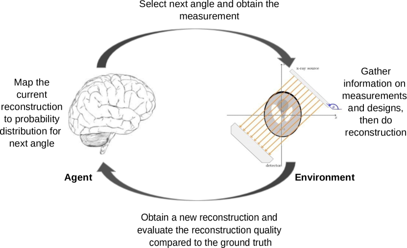
The structure of this paper is as follows. In section \@slowromancapii@, we present the background on CT reconstruction, Bayesian OED, and reinforcement learning. In section \@slowromancapiii@, we discuss the formulation of this experimental design as a POMDP and describe the computation of the policy gradient using the Actor-Critic approach. We provide a set of numerical experiments in section \@slowromancapiv@ to assess the performance of our proposed method. Finally, in section \@slowromancapv@ and section \@slowromancapvi@, we discuss and summarize our findings.
II Background
II-A CT Reconstruction
In sparse-angle tomography, the challenge lies in accurately reconstructing an image from incomplete measurement data, where only a limited number of angles are acquired. This inverse problem is severely ill-posed, meaning that small errors in the measurements could result in a large reconstruction error, or that several reconstructions are consistent with the measurements [18]. The Filtered Back-Projection (FBP) algorithm, a traditional analytical reconstruction method, has limitations when used for sparse-angle tomography. It assumes that the measurements are acquired with low noise over the full angular range, resulting in inferior reconstructions when applied to limited data [19].
To address this challenge, it is necessary to incorporate prior information into the reconstruction algorithm to compensate for the limited data [20, 19]. Regularised algebraic reconstruction methods have been proposed to incorporate such prior information efficiently. When applied to limited data, these can result in more stable and accurate reconstructions.
Therefore, we represent the object that we would like to reconstruct as where represents the number of pixels or voxels. A single noisy measurement at angle is generated as
| (1) |
with and is a discretization of the Radon transform along angle .
The reconstructed image from measurements along angles is obtained via
| (2) |
where is a regularization term representing prior information for .
II-B Bayesian OED
Bayesian OED is a statistical framework that optimizes the design of an experiment by trading off the information gain with the cost of an experiment.
In the context of X-ray CT experimental design, the utility function in Bayesian OED measures the reconstruction quality, where the true underlying ground truth is estimated by from measurements obtained under experimental conditions specified by . The optimal design maximizes the expectation of the utility function over the design space with respect to the measured data and the model parameter .
Sequential OED is an approach that adjusts the design parameters as new data is acquired. This is achieved by treating the experiment as a sequential decision-making process, where the aim is to select the most informative design parameters based on the observed data to maximize the utility function. In the step of an X-ray CT experiment, the process involves generating observed data using a data model (as shown in Equation (1)), updating the posterior distribution of given the observed data up to step (denoted by in Equation (2)), obtaining the reconstruction for the underlying ground truth. Subsequently, the most informative angle is selected as the next design parameter to be used, which maximizes the utility function.
II-C Reinforcement Learning
Reinforcement learning is a widely used approach for sequential decision-making, allowing agents to learn how to map the current state to actions that maximize the total reward for the entire process [21]. Since it considers the long-term effects of actions, reinforcement learning can realize non-greedy sequential decision-making. This approach is based on the Markov Decision Processes (MDPs) framework , which consists of a set of states , a set of actions , a transition operator representing the conditional probability distribution from the current state to the next state after selecting an action, and a reward function: that provides feedback from the environment at each time step.
A policy in reinforcement learning is a mapping from the current state to a probability distribution of actions: .
In MDPs with a finite number of states, the process begins from an initial state with a probability distribution . The agent follows a policy that maps the initial state to the first action, leading the agent to transition to the next state and receive a reward from the environment. This process is repeated until a terminal state is reached, generating a trajectory or an episode of steps.
In practical applications, the problems encountered may not conform to the idealized framework of a reinforcement learning problem. To address this, POMDPs are utilized. A POMDP can be defined as a tuple , where two additional components are included in addition to the ones in the standard MDP formulation: a finite observation set and an observation function that defines the conditional probability distribution over the observation in the underlying state after executing an action. Since the agent has limited knowledge about the underlying state in POMDPs, the policy must either map historical observations to the next action or extract information from historical observations in the form of a belief state.
Reinforcement learning aims to find the optimal policy with parameters , denoted as , that generates the trajectory or episode to maximize the expected total reward. The objective function for reinforcement learning can be expressed as follows:
| (3) | ||||
The objective function measures the expected total reward with a discount factor to account for future uncertainty, and represents the trajectory generation process by the policy.
The total rewards for one trajectory are obtained after the agent completes an episode. The expectation over all trajectories can be estimated by sampling many trajectories. To enhance the process’s efficiency, some reinforcement learning approaches utilize value functions that evaluate the expected future benefits from the step following the policy. The state-value function quantifies the expected cumulative reward from state , taking into account all possible trajectories following the current policy that start from this state.
III Methods
III-A Sequential OED as a POMDP
We take the reconstruction as a belief state rather than considering measurements as the state, as done in [17]. To formulate the problem, we adopt a Bayesian OED framework and model it as a POMDP. The POMDP formulation for the X-ray CT experiment is defined as follows:
-
•
Observation space : The observation space is defined as the set of measurements generated by the data model expressed in Equation (1).
-
•
State space : The ground truth represents the underlying state. The current reconstruction (belief state) of the underlying state, denoted by , is obtained using the SIRT algorithm with box constraints [22] as specified in Equation (2). For ease of notation, we use to represent the reconstruction at the step. In addition, we maintain a vector to keep track of the angles that have been selected before the experiment to prevent repeating the same angles.
-
•
Action space : The action space is a discrete design space consisting of 180 integer angles from the range .
-
•
Transition function and observation function : The transition function is deterministic, as the underlying state remains unchanged. On the other hand, the data model given by Equation (1) serves as the observation function, from which we only consider measurement samples.
-
•
Reward function : The reward function is defined based on the PSNR value between the reconstruction obtained after selecting the angle and its ground truth. Two reward settings are considered, both of which correspond to A-optimality in Bayesian OED.:
-
–
End-to-end setting: The reward is given as follows:
If the fixed number of angles is reached, the episode terminates, and the final PSNR value is given. Otherwise, the agent receives a reward of .
-
–
Incremental setting: The reward is given as follows:
The reward represents the improvement in the current reconstruction quality compared to the previous step.
-
–
III-B Actor-Critic method for policy optimization
The Actor-Critic method is a novel category in the field of reinforcement learning for computing the policy gradient on the objective function described in Equation (3). The proposed approach leverages the concept of value functions and utilizes a state-value function to obtain the expected future rewards at the current state, thereby expediting the learning process. Additionally, this method parameterizes the value function. The Temporal-Difference (TD) error [21] is employed in this approach, which calculates the discrepancy between the estimated value function for the current state and the sum of the current reward and the discounted estimated value function for the next state. This enables the state-value function to be updated through bootstrapping and provides a direction for policy gradient.
At the beginning of each episode, a zero matrix and a zero vector are used as the initial state and action vector, respectively. The complete algorithm is presented in Algorithm (1).
III-C Network architecture
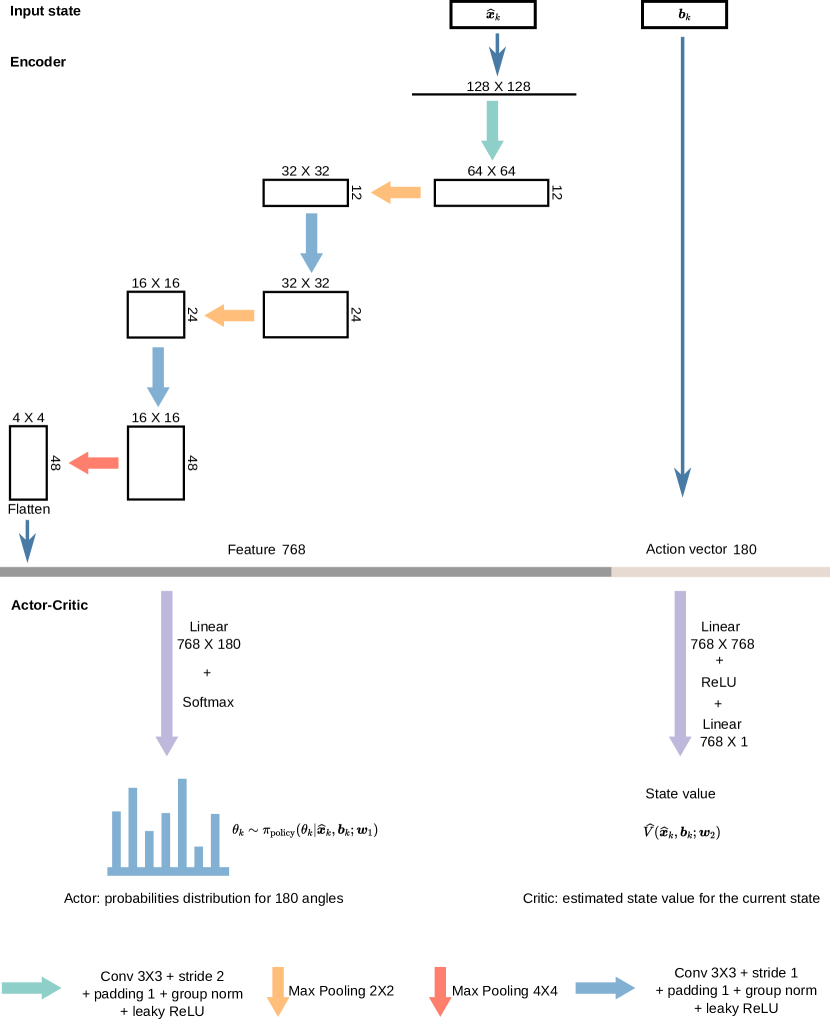
The proposed method requires the agent to extract relevant features from high-dimensional images to increase learning efficiency, which is accomplished using a deep neural encoder network. The architecture of the encoder network and the Actor-Critic network is shown in Figure (2), with the input image being of dimension . The neural network’s connection weights represent the policy parameters and the state-value function parameters .
The proposed model adopts a shared encoder network between the actor and critic networks. This shared encoder network comprises three convolutional neural networks (CNNs) each with padding and group normalization, followed by a leaky Rectified Linear Unit (ReLU) activation and a max pooling operation for down-sampling. The shared encoder network consists of a total of 13,320 parameters. Furthermore, the following actor and critic networks are separate and have 170,820 and 900,601 parameters, respectively.
Figure (2) outlines the process by which the network operates in the context of the actor-critic method. The encoder network takes the reconstruction as input and produces a feature vector in the bottleneck layer, which is flattened into a 1D vector and concatenated with the 1D action vector . The resulting information is then fed into the following actor and critic networks.
The actor network uses a Soft-max policy to map the information to a probability distribution over all possible angle candidates in the action space, while the critic network estimates the state-value function . Based on the probability distribution generated by the actor network, the agent selects the next angle and subsequently collects measurements to obtain a new reconstruction . The action vector is updated as accordingly.
To compute the policy gradient and update the parameters in the value function using TD error in Algorithm (1), the new reconstruction and the new action vector are fed into the network again. This is done to calculate a new state-value function . Once an angle is selected, both the policy parameters and the value function parameters are updated once.
IV Numerical Experiments
We examine in intuitive numerical experiments whether the learned policies are really able to sequentially adapt the scan angles to the object (a-posteriori adaptation). For this, we use various simple numerical phantoms for which the informative angles are well-known. Throughout our experiments, we focus on parallel-beam geometry and simple 2D tomography using synthetic data. The code and synthetic data are available on Github 111https://github.com/tianyuan1wang/SeqAngleRL.
IV-A Data sets
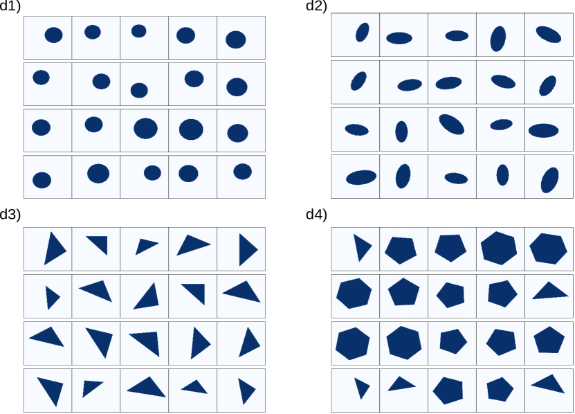
In our numerical experiments, we consider several shapes depicted in Figure (3). All phantoms in the data sets have a size of and are binary images. To assess the adaptability of the agent to dynamic environments, each data set includes phantoms with different rotations, causing a shift in their informative angles. These rotations are represented by 36 equally spaced angles ranging from to . Additionally, the phantoms in each data set exhibit various scaling and shifts. Nonetheless, these modifications do not alter the informative angles, thereby preserving the consistency of informative angles across the scaled and shifted phantoms. By including these scaling and shifts, we aim to ensure the agent’s ability to recognize the same object despite its size and location variations.
d1) Circles: The first data set consists of circles with varying locations and radii. Due to its uniform curvature, a circle does not have a relatively higher concentration of informative angles. To obtain an accurate reconstruction, angles must be equidistantly distributed.
d2) Ellipses: Unlike circles, ellipses have a major axis and a minor axis. The major axis serves as a preferential direction, making angles around it more informative, as shown in references [7] and [23].
d3) Triangles: Triangles, characterized by one angle of and two angles of , possess three preferential directions, causing the informative angles to be tangential to their edges.
d4) Mixed phantoms: The final data set consists of a mixture of phantoms, including triangles from d3), regular pentagons, and regular hexagons, each of which has its own preferential directions.
IV-B Implementation
For all of our experiments, the sequential experimental process for each data set in Figure (3) follows Algorithm (1). To generate the measurement data, we utilize the ASTRA Toolbox [24, 25], considering a projection size of . The reconstruction is performed using the SIRT algorithm with box constraints [0,1] for 150 iterations.
The encoder and Actor-Critic neural network architectures are illustrated in Figure (2). During training, we set the discount factor to 0.99 and assign weights of 1.0 and 0.5 to the actor loss and critic loss, respectively. To encourage exploration during training, we incorporate an entropy loss with a weight of 0.01. For optimization of the parameters, we employ the Adam optimizer [26] with a learning rate of and weight decay of .
The number of phantoms used for training differs between experiments, with experiments d1) to d3) consisting of 3,000 training phantoms, while experiment d) has 9,000 training phantoms. the number of episodes required for convergence during training also varies among experiments, with experiment d1) requiring 100,000 episodes, experiments d2) and d3) requiring 150,000 episodes, and experiment d4) requiring 300,000 episodes.
To assess the generalization ability of the Actor-Critic agent, a set of testing experiments for d2) to d4) is performed to evaluate its ability to identify previously unseen rotations of phantoms, representing out-of-distribution data. The number of test phantoms varies across the conducted experiments, denoted as d2) to d4). Specifically, 300 test phantoms are used in experiments d2) and d3), while 900 are used in experiments d4).
In addition, we consider two reward functions: incremental and end-to-end settings. An equidistant policy is introduced as a benchmark to compare the performance of the Actor-Critic policy with un-informed and non-adaptive angle selection method.
The subsequent sections will present the training and testing outcomes on the aforementioned data set and compare the Actor-Critic policies utilizing two reward settings and the equidistant policy.
IV-C Experiment 1 - Uniform informative angles
In the first experiment, we aim to evaluate the performance of the Actor-Critic policy on the circles data set, which have a uniform distribution of informative angles. It is known that the equidistant benchmark is the optimal policy for this data set. Our objective is to investigate whether the Actor-Critic policy approaches the equidistant policy in performance.
As depicted in Figure (4), the equidistant policy exhibits enhanced performance for the circular phantoms compared to the Actor-Critic policies with diverse reward configurations. Furthermore, we observed that the performance of the Actor-Critic policy with end-to-end reward surpasses that of the policy with incremental reward as the number of angles increases.
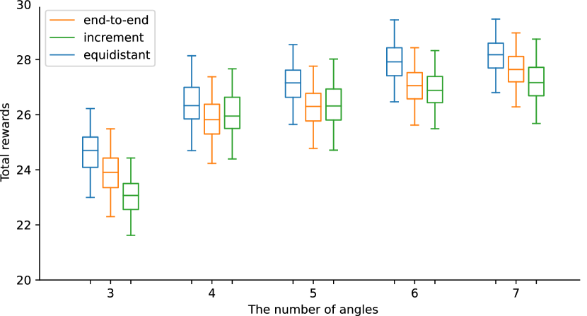
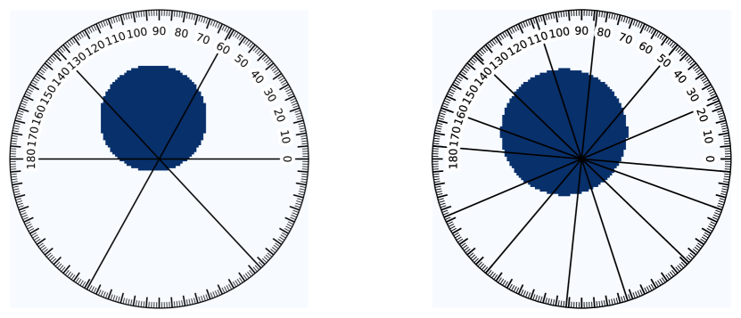
Figure (5) presents two samples considering three and seven angles obtained from the Actor-Critic policy with the end-to-end reward setting. This result demonstrates that the Actor-Critic agent tends to distribute the selected angles evenly, although the number of angles is different.
IV-D Experiment 2 - Non-uniform informative angles
In contrast to circles, informative angles in ellipses are found to be concentrated around its major axis.
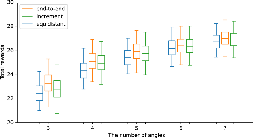
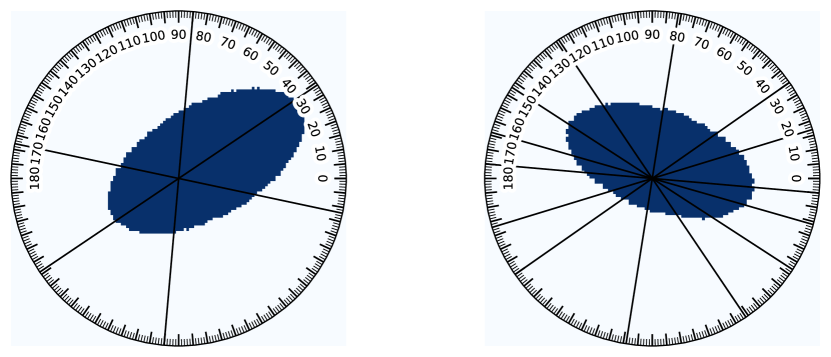
The training outcomes of the ellipse phantoms over the final 2,000 episodes are shown in Figure (6), which indicates that the Actor-Critic policies exhibit superior performance. As the number of angles increases, the results for the three policies get closer. This is because a sufficient number of angles around the major axis have already been obtained, even for the equidistant policy, to achieve a high-quality reconstruction. Notably, the Actor-Critic policy with the end-to-end reward setting achieves the best performance. Figure (7) presents the results for two ellipse phantoms, demonstrating that the agent can discern the rotation of the ellipse and concentrate the distribution of the angles around the informative area. As the number of angles increases, the agent increases the number of angles around the major axis.
Table (LABEL:tb:EllipseTest) reports the test outcomes for the ellipses data set with three to seven angles. Consistent with the training results, the Actor-Critic policies demonstrate superior performance compared to the benchmark, with the policies becoming progressively closer as the number of angles increases. The end-to-end reward setting still shows the best average performance, though it has a higher variance.
| Policies | 3 | 4 | 5 | 6 | 7 |
|---|---|---|---|---|---|
| Learned adaptive policy (end-to-end) | 23.16 1.02 | 25.10 0.72 | 25.73 1.20 | 26.31 0.82 | 26.87 1.06 |
| Learned adaptive policy (increment) | 22.78 0.92 | 24.90 0.73 | 25.67 0.77 | 26.33 0.79 | 26.86 0.73 |
| Equidistant policy | 22.40 0.74 | 24.27 0.73 | 25.35 0.69 | 26.16 0.64 | 26.73 0.62 |
IV-E Experiment 3 - Explicit informative angles
The third experiment focuses on evaluating the ability of the Actor-Critic agent to identify explicit informative angles for phantoms with sharp edges, namely triangles. These phantoms have well-defined informative angles that are tangential to their edges, and thus, it is of interest to investigate if the agent can successfully locate these angles. The results of this experiment will provide insight into the performance of the Actor-Critic agent in detecting preferential directions for phantoms with sharp edges.
In this study, a fixed number of five angles is employed. As shown in Figure (8), both reward settings for the Actor-Critic agent outperform the equidistant policy. Specifically, training using the incremental reward setting demonstrates faster convergence, whereas the end-to-end reward setting yields the best performance.
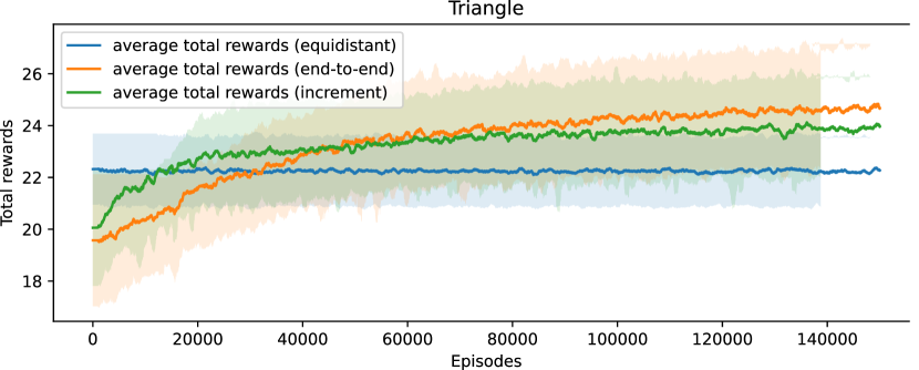
The training results demonstrate that the Actor-Critic agent tends to select the first two angles as fixed angles, with particular emphasis on the first angle, while the second angle exhibits some uncertainty. Subsequently, the agent would select three informative angles to optimize the reconstruction process. This behavior is consistent with the fact that the initial state is set as a zero matrix and a zero vector with no prior information, and the agent, therefore, prioritizes gathering information by fixing the first angle or first two angles before personalizing the strategies based on the different phantoms encountered.
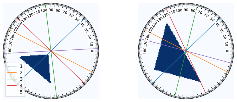
Figure (9) presents two samples of the agent’s performance in an end-to-end reward setting, in which the agent selects the initial two angles of and . Subsequently, for the right phantom, the agent selects , , and as the following three angles, while for the left phantom, the agent chooses , , and . Notably, these angles are almost tangential to the edges of the triangle phantoms.
We observe that the agent tends to select more angles around the informative angles or repeat its selection when the first two angles are close to the informative angles. Again, this behavior can be explained by the informative angles containing the most relevant information for accurate reconstruction.
| Policies | Triangles |
|---|---|
| Learned adaptive policy (end-to-end) | 24.07 2.07 |
| Learned adaptive policy (increment) | 23.78 1.80 |
| Equidistant policy | 20.64 1.05 |
In regards to the out-of-distribution test, Table (LABEL:tb:TriangleTest) demonstrates that the Actor-Critic policies outperform the equidistant benchmark. Furthermore, it is observed that the end-to-end reward setting achieves the highest quality in terms of reconstruction.
IV-F Experiment 4 - Mixed phantoms with explicit informative angles
In this study, we aim to investigate the capacity of an Actor-Critic agent to recognize and distinguish between different phantoms with varying informative angles and their rotation. In this study, a fixed number of seven angles is employed.
Similar to Experiment 3, shown in Figure (10), the training for the mixed phantoms reveals that the incremental reward setting facilitates faster convergence, while end-to-end reward setting results in better performance. Figure (11) illustrates the performance of the end-to-end reward setting. It fixes the first two angles to and for the hexagon and triangle, respectively, while it selects and for the pentagon as the first two angles because of some uncertainty for the second angle as mentioned in Experiment 3. The agent then selects the subsequent informative angles based on this prior information by the fixed angles.
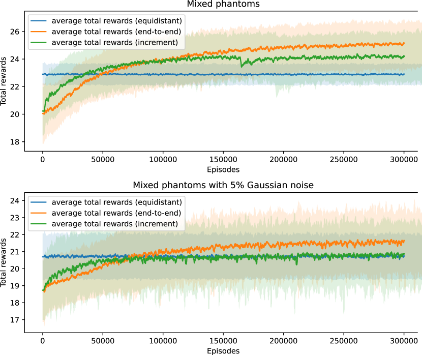
Furthermore,we investigate the impact of Gaussian noise on an Actor-Critic agent’s ability to select informative angles for phantoms. Our results, presented in Figure (10), demonstrate that the performance gap between the equidistant and Actor-Critic policies is reduced in the presence of Gaussian noise on the measurements. Specifically, our training results show that the incremental reward setting yields nearly identical total rewards to the equidistant policy, suggesting that the presence of noise negatively impacts the training process. Additionally, comparing the result samples from end-to-end rewards in Figures (11) and (12), we find that the noise in measurements has a substantial influence on the angle selection strategy, including the fixed angles and the informative angles selection orders afterward. To better understand the differences between the two policies in Figures (11) and (12), we show the policy results for triangles in Figure (13). Our analysis reveals that the policy for clean data is tightly clustered around informative angles, whereas the policy for noisy data is more broadly distributed. We also observe that the policy realizes adaptive angle selection, where the probability of a chosen angle decreases significantly, followed by an increase in the probability of some angles with a small probability.


Based on the results for the PSNR values presented in Table (LABEL:tb:MixedTest), it can be observed that the Actor-Critic policies, with both end-to-end and incremental rewards, outperform the equidistant policy. In addition, adding noise to the measurements reduces the performance gap between the policies. Notably, the end-to-end reward setting still exhibits the highest performance. Moreover, the model’s performance on noisy measurements improves when testing the model trained on clean measurements compared to the model trained on noisy measurements, confirming that the training on noisy measurements degrade the performance of the Actor-Critic policies.
| Policies | Mixed phantoms | Mixed phantoms (5%) | Mixed phantoms (5%) - clean training |
|---|---|---|---|
| Learned adaptive policy (end-to-end) | 24.85 1.64 | 21.52 1.63 | 21.82 1.83 |
| Learned adaptive policy (increment) | 24.15 1.55 | 20.98 1.75 | 21.56 1.80 |
| Equidistant policy | 22.94 0.76 | 20.75 1.37 | 20.75 1.37 |
V Discussion
The results demonstrate that for classes of phantoms with a clear informative angles, the reinforcement learning policy are able to achieve superior performance compared to the uninformed, equidistant policy. As the informative angles were differing for each individual phantom and were not shared along the whole class of phantoms, no informative angles could be known a-priori. We therefore demonstrated that the policies learned truly preform a-posteriori adaptation. This complements the findings from [17], whose numerical studies could not answer this important question.
Importantly, the trained reinforcement learning policies exhibit generalization capabilities on the test dataset, including rotations not encountered during training. Interestingly, adding measurement noise reduces the achievable gains in performance, and understanding and mitigating the reason for this will be a topic for future research.
In addition, we conducted numerical experiments to compare end-to-end and incremental reward functions. The end-to-end reward function achieves the highest average performance on both the training and test datasets. This indicates its effectiveness in guiding the reinforcement learning agent toward optimal solutions. On the other hand, the incremental reward function demonstrates faster convergence during training. In the future, we will investigate further how to design reward functions that share both of these desirable properties.
In the future, our work can be extended in the following ways: Firstly, instead of using SIRT as an image reconstruction method, we will use deep learning-based reconstruction methods, trained end-to-end. Secondly, more complex reward functions can be designed to achieve task-specific angle selection. For example, to detect defects in in-line quality control, one could reward angle selection policies that improve the contrast between the defect and its embedding. Thirdly, we restricted ourselves to a simple 2D parallel-beam geometry to obtain scenarios in which optimal angle selection strategies are known, and the results of trained policies can be interpreted more easily. In the future, we will extend the approach to more complex and realistic 3D geometries with additional degrees of freedom, such as tilting and zooming.
VI Conclusion
Compared to classical, computationally prohibitive approaches to solve the sequential OED problem of adaptive angle selection in X-ray CT, deep reinforcement learning avoids direct gradient computation on the high-dimensional, non-convex, bi-level optimization problem. Instead, it learns non-greedy strategies to solve it for a particular class of phantoms during an offline training phase which can then be applied fast and efficiently online to scans of new phantoms. We posed the sequential OED problem as a POMDP and utilized the Actor-Critic network combining a shared encoder network to learn an optimal policy. In our numerical studies with 2D CT scenarios mimicking industrial, in-line CT inspection, we could demonstrate that our approach learns efficient, truly adaptive policies that achieve better performance in terms of reconstruction quality. We introduced two different reward function settings, namely, the end-to-end and incremental reward settings. Both settings lead to stable learning processes, consolidating reinforcement learning as a reliable and extremely promising method for sequential OED. To conclude, our work demonstrates the potential of using reinforcement learning for solving sequential OED problems in inverse problems and imaging - in particular to automate angle selection and improve CT imaging efficiency, providing a flexible and adaptive approach for various CT imaging scenarios in the Industry 4.0.
Acknowledgement
This research was co-financed by the European Union H2020-MSCA-ITN-2020 under grant agreement no. 956172 (xCTing). We would like to express our gratitude to Chat Generative Pre-trained Transformer (ChatGPT) for its assistance in refining the English writing of this paper.
References
- [1] I. Kazantsev, “Information content of projections,” Inverse problems, vol. 7, no. 6, p. 887, 1991.
- [2] L. Varga, P. Balázs, and A. Nagy, “Projection selection dependency in binary tomography,” Acta Cybernetica, vol. 20, no. 1, pp. 167–187, 2011.
- [3] L. Ruthotto, J. Chung, and M. Chung, “Optimal experimental design for inverse problems with state constraints,” SIAM Journal on Scientific Computing, vol. 40, no. 4, pp. B1080–B1100, 2018.
- [4] D. V. Lindley, Bayesian statistics: A review. SIAM, 1972.
- [5] E. Ryan, C. Drovandi, J. McGree, and A. Pettitt, “Fully bayesian optimal experimental design: A review,” International Statistical Review, vol. 84, pp. 128–154, 2016.
- [6] M. Burger, A. Hauptmann, T. Helin, N. Hyvönen, and J.-P. Puska, “Sequentially optimized projections in x-ray imaging,” Inverse Problems, vol. 37, no. 7, p. 075006, 2021.
- [7] K. J. Batenburg, W. J. Palenstijn, P. Balázs, and J. Sijbers, “Dynamic angle selection in binary tomography,” Computer Vision and Image Understanding, vol. 117, no. 4, pp. 306–318, 2013.
- [8] A. Dabravolski, K. J. Batenburg, and J. Sijbers, “Dynamic angle selection in x-ray computed tomography,” Nuclear Instruments and Methods in Physics Research Section B: Beam Interactions with Materials and Atoms, vol. 324, pp. 17–24, 2014.
- [9] K. J. Batenburg, W. Fortes, L. Hajdu, and R. Tijdeman, “Bounds on the difference between reconstructions in binary tomography,” in International Conference on Discrete Geometry for Computer Imagery. Springer, 2011, pp. 369–380.
- [10] T. Helin, N. Hyvönen, and J.-P. Puska, “Edge-promoting adaptive bayesian experimental design for x-ray imaging,” SIAM Journal on Scientific Computing, vol. 44, no. 3, pp. B506–B530, 2022.
- [11] R. Barbano, J. Leuschner, J. Antorán, B. Jin, and J. M. Hernández-Lobato, “Bayesian experimental design for computed tomography with the linearised deep image prior,” arXiv preprint arXiv:2207.05714, 2022.
- [12] A. Fischer, T. Lasser, M. Schrapp, J. Stephan, and P. B. Noël, “Object specific trajectory optimization for industrial x-ray computed tomography,” Scientific reports, vol. 6, no. 1, pp. 1–9, 2016.
- [13] J. W. Stayman and J. H. Siewerdsen, “Task-based trajectories in iteratively reconstructed interventional cone-beam ct,” Proc. 12th Int. Meet. Fully Three-Dimensional Image Reconstr. Radiol. Nucl. Med, pp. 257–260, 2013.
- [14] G. Herl, J. Hiller, M. Thies, J.-N. Zaech, M. Unberath, and A. Maier, “Task-specific trajectory optimisation for twin-robotic x-ray tomography,” IEEE Transactions on Computational Imaging, vol. 7, pp. 894–907, 2021.
- [15] B. Victor, C. Vienne, and V. Kaftandjian, “Fast algorithms based on empirical interpolation methods for selecting best projections in sparse-view x-ray computed tomography using a priori information,” Available at SSRN 4170496.
- [16] F. Bauer, D. Forndran, T. Schromm, and C. U. Grosse, “Practical part-specific trajectory optimization for robot-guided inspection via computed tomography,” Journal of Nondestructive Evaluation, vol. 41, no. 3, p. 55, 2022.
- [17] Z. Shen, Y. Wang, D. Wu, X. Yang, and B. Dong, “Learning to scan: A deep reinforcement learning approach for personalized scanning in ct imaging,” Inverse Problems & Imaging, vol. 16, no. 1, 2022.
- [18] J. L. Mueller and S. Siltanen, Linear and nonlinear inverse problems with practical applications. SIAM, 2012.
- [19] P. C. Hansen, J. Jørgensen, and W. R. Lionheart, Computed Tomography: Algorithms, Insight, and Just Enough Theory. SIAM, 2021.
- [20] T. M. Buzug, Computed tomography. Springer, 2011.
- [21] R. S. Sutton and A. G. Barto, Reinforcement learning: An introduction. MIT press, 2018.
- [22] T. Elfving, P. C. Hansen, and T. Nikazad, “Semiconvergence and relaxation parameters for projected sirt algorithms,” SIAM Journal on Scientific Computing, vol. 34, no. 4, pp. A2000–A2017, 2012.
- [23] M. Venere, H. Liao, and A. Clausse, “A genetic algorithm for adaptive tomography of elliptical objects,” IEEE Signal Processing Letters, vol. 7, no. 7, pp. 176–178, 2000.
- [24] W. Van Aarle, W. J. Palenstijn, J. De Beenhouwer, T. Altantzis, S. Bals, K. J. Batenburg, and J. Sijbers, “The astra toolbox: A platform for advanced algorithm development in electron tomography,” Ultramicroscopy, vol. 157, pp. 35–47, 2015.
- [25] W. Van Aarle, W. J. Palenstijn, J. Cant, E. Janssens, F. Bleichrodt, A. Dabravolski, J. De Beenhouwer, K. J. Batenburg, and J. Sijbers, “Fast and flexible x-ray tomography using the astra toolbox,” Optics express, vol. 24, no. 22, pp. 25 129–25 147, 2016.
- [26] D. P. Kingma and J. Ba, “Adam: A method for stochastic optimization,” arXiv preprint arXiv:1412.6980, 2014.
VII Biography Section
| Tianyuan Wang received a Bsc. in Automation from Central South University in China and a Msc. in Computer Engineering from RWTH Aachen University in Germany. Currently, he is working as a Ph.D. student in the Computational Imaging group of the Centrum Wiskunde Informatics (CWI) in the Netherlands. His research is part of the xCTing network and aims to realize adaptive angle selection for in-line CT. |
| Felix Lucka is a senior researcher in the Computational Imaging group at the Centrum Wiskunde Informatica (CWI). After obtaining a first degree in mathematics and physics in 2011, he completed a PhD in applied mathematics at WWU Münster (Germany) in 2015 followed by a postdoc at University College London until 2017. His main interests are mathematical challenges arising from biomedical imaging applications that have a classical inverse problem described by partial differential equations at their core. |
| Tristan van Leeuwen is the group leader of the Computational Imaging group at the Centrum Wiskunde Informatica (CWI) in the Netherlands. He received his BSc. and MSc. in Computational Science from Utrecht University. He obtained his PhD. in geophysics at Delft University in 2010. After spending some time as a postdoctoral researcher at the University of British Columbia in Vancouver, Canada and the CWI, he returned to Utrecht University in 2014 as an assistant professor at the mathematical institute. In 2021, he moved to his current position. His research interests include: inverse problems, computational imaging, tomography and numerical optimization. |