Provably Faster Gradient Descent via Long Steps

Benjamin Grimmer111Johns Hopkins University, Department of Applied Mathematics and Statistics, grimmer@jhu.edu
Abstract

This work establishes new convergence guarantees for gradient descent in smooth convex optimization via a computer-assisted analysis technique. Our theory allows nonconstant stepsize policies with frequent long steps potentially violating descent by analyzing the overall effect of many iterations at once rather than the typical one-iteration inductions used in most first-order method analyses. We show that long steps, which may increase the objective value in the short term, lead to provably faster convergence in the long term. A conjecture towards proving a faster O(1/TlogT)𝑂1𝑇𝑇O(1/T\log T) rate for gradient descent is also motivated along with simple numerical validation.

1 Introduction

This work proposes a new analysis technique for gradient descent, establishing a path toward provably better convergence guarantees for smooth, convex optimization than is possible with existing approaches based on constant stepsizes. Instead, our theory allows for nonconstant stepsize policies, periodically taking larger steps that may violate the monotone decrease in objective value typically needed by analysis. In fact, contrary to the common intuition, we show periodic long steps, which may increase the objective value in the short term, provably speed up convergence in the long term, with increasingly large gains as longer and longer steps are periodically included. This bears a similarity to accelerated momentum methods, which also depart from ensuring a monotone objective decrease at every iteration.

Establishing this requires a proof technique capable of analyzing the overall effect of many iterations at once rather than the typical (naive) one-iteration inductions used in most first-order method analyses. Our proofs are based on the Performance Estimation Problem (PEP) ideas of [1, 2, 3], which cast computing/bounding the worst-case problem instance of a given algorithm as a Semidefinite Program (SDP). We show that the existence of a feasible solution to a related SDP proves a descent guarantee after applying a corresponding pattern of nonconstant stepsizes, from which faster convergence guarantees follow. Our technique is very similar to that first proposed by Altschuler’s Master’s thesis [4, Chapter 8] which established repeating stepsize patterns of length two or three with faster contractions towards the minimizer for smooth, strongly convex minimization. Most existing PEP literature uses computer-solves to guide the search for tighter convergence proofs [5, 3, 6, 7, 8, 9, 10, 11, 12, 13] and inform the development of new, provably faster algorithms [14, 15, 16, 17, 18]. Here computer outputs are directly used to constitute the proof, but are large (up to tens of thousands of rational numbers) and so may provide less guidance or intuition.

We consider gradient descent with a sequence of (normalized) stepsizes h=(h0,h1,h2,)subscript0subscript1subscript2h=(h_{0},h_{1},h_{2},\dots) applied to minimize a convex function f:n:𝑓superscript𝑛f\colon\mathbb{R}^{n}\rightarrow\mathbb{R} with L𝐿L-Lipschitz gradient by iterating

xk+1=xkhkLf(xk)subscript𝑥𝑘1subscript𝑥𝑘subscript𝑘𝐿𝑓subscript𝑥𝑘x_{k+1}=x_{k}-\frac{h_{k}}{L}\nabla f(x_{k}) (1.1)

given an initialization x0nsubscript𝑥0superscript𝑛x_{0}\in\mathbb{R}^{n}. We assume throughout that a minimizer xsubscript𝑥x_{\star} of f𝑓f exists and its level sets are bounded D=sup{xx2f(x)f(x0)}𝐷supremumconditionalsubscriptnorm𝑥subscript𝑥2𝑓𝑥𝑓subscript𝑥0D=\sup\{\|x-x_{\star}\|_{2}\mid f(x)\leq f(x_{0})\}222This assumption can likely be relaxed but eases our development herein.. The classic convergence guarantee [19] for gradient descent is that with constant stepsizes h=(1,1,1,)111h=(1,1,1,\dots), every T>0𝑇0T>0 has f(xT)f(x)LD2/2(T+1)𝑓subscript𝑥𝑇𝑓subscript𝑥𝐿superscript𝐷22𝑇1f(x_{T})-f(x_{\star})\leq LD^{2}/2(T+1). Using performance estimation techniques, a tight refinement of this bound was given by [1, Theorem 3.1] (and elementary proof, avoiding the use of PEP, was given by [20]): every T>0𝑇0T>0 has

f(xT)f(x)LD24T+2.𝑓subscript𝑥𝑇𝑓subscript𝑥𝐿superscript𝐷24𝑇2f(x_{T})-f(x_{\star})\leq\frac{LD^{2}}{4T+2}\ . (1.2)

By tight, we mean a matching problem instance exists that attains the above inequality. Using stepsizes between one and two, this rate can be improved by another factor of two (see [2, 20]). Stepsizes beyond length two have very little prior theory as one can no longer guarantee a decrease in objective value at each iteration.

Here we provide an analysis technique capable of handling nonconstant stepsizes, periodically longer than one can guarantee descent for, finding increasingly fast convergence (in terms of constants) follows. For example, consider gradient descent alternating stepsizes h=(2.9,1.5, 2.9,1.5,)2.91.52.91.5h=(2.9,1.5,\ 2.9,1.5,\ \dots). Such a scheme is beyond the reach of traditional descent-based analysis as one may fear the stepsizes of 2.92.92.9 can increase the function value individually more than the 1.51.51.5 is guaranteed to decrease it. Regardless, we show this “long step” converges with

f(xT)f(x)LD22.2×T+O(1/T2)𝑓subscript𝑥𝑇𝑓subscript𝑥𝐿superscript𝐷22.2𝑇𝑂1superscript𝑇2f(x_{T})-f(x_{\star})\leq\frac{LD^{2}}{2.2\times T}+O(1/T^{2})

for every even T>0𝑇0T>0. See our Theorem 3.2 characterizing many such alternating stepsize methods. The +O(1/T2)𝑂1superscript𝑇2+O(1/T^{2}) terms throughout this work are only used to suppress two universal constants, namely above, we show there exist constants s¯¯𝑠\bar{s} and C𝐶C such that all even T>2s¯𝑇2¯𝑠T>2\bar{s} have bound LD2/(2.2×TC)𝐿superscript𝐷22.2𝑇𝐶LD^{2}/(2.2\times T-C).

Using longer cycles, we derive further performance gains. For example, we show a carefully selected stepsize pattern of length 127127127 periodically taking stepsizes of 370.0370.0370.0 converges at a rate of LD2/(5.8346303×T)𝐿superscript𝐷25.8346303𝑇LD^{2}/(5.8346303\times T). Generally, given a stepsize pattern h=(h0,,ht1)tsubscript0subscript𝑡1superscript𝑡h=(h_{0},\dots,h_{t-1})\in\mathbb{R}^{t}, we consider the gradient descent method repeatedly applying the pattern of stepsizes

xk+1=xkh(k𝚖𝚘𝚍t)Lf(xk).subscript𝑥𝑘1subscript𝑥𝑘subscript𝑘𝚖𝚘𝚍𝑡𝐿𝑓subscript𝑥𝑘x_{k+1}=x_{k}-\frac{h_{(k\mathtt{\ mod\ }t)}}{L}\nabla f(x_{k})\ . (1.3)

In Theorem 2.1, we give a convergence guarantee for any straightforward stepsize pattern hh of

f(xT)f(x)LD2avg(h)T+O(1/T2)𝑓subscript𝑥𝑇𝑓subscript𝑥𝐿superscript𝐷2avg𝑇𝑂1superscript𝑇2f(x_{T})-f(x_{\star})\leq\frac{LD^{2}}{\mathrm{avg}(h)T}+O(1/T^{2}) (1.4)

where avg(h)=1ti=0t1hiavg1𝑡superscriptsubscript𝑖0𝑡1subscript𝑖\mathrm{avg}(h)=\frac{1}{t}\sum_{i=0}^{t-1}h_{i}. See Section 2 for the formal introduction of this straightforwardness property. Hence the design of provably faster nonconstant stepsize gradient descent methods amounts to seeking straightforward stepsize patterns with large average stepsize values. Certifying a given pattern is straightforward can be done via semidefinite programming (see our Theorem 3.1). So the convergence analysis of such nonconstant stepsizes methods is a natural candidate for computer assistance.

Pattern Length “Straightforward” Stepsize Pattern hh
(longest stepsize marked in bold)
Convergence Rate
(+O(1/T2)𝑂1superscript𝑇2+O(1/T^{2}) omitted)
t=2𝑡2t=2 (𝟑η,1.5)for any η(0,3)3𝜂1.5for any 𝜂03({\bf 3-\eta},1.5)\qquad\text{for\ any\ }\eta\in(0,3) LD2(2.25η/2)×T𝐿superscript𝐷22.25𝜂2𝑇\dfrac{LD^{2}}{(2.25-\eta/2)\times T}
t=3𝑡3t=3 (1.5,4.9,1.5)1.54.91.5(1.5,{\bf 4.9},1.5) LD22.63333×T𝐿superscript𝐷22.63333𝑇\dfrac{LD^{2}}{2.63333...\times T}
t=7𝑡7t=7 (1.5,2.2,1.5,12.0,1.5,2.2,1.5)1.52.21.512.01.52.21.5(1.5,2.2,1.5,{\bf 12.0},1.5,2.2,1.5) LD23.1999999×T𝐿superscript𝐷23.1999999𝑇\dfrac{LD^{2}}{3.1999999\times T}
t=15𝑡15t=15 (1.4,2.0,1.4,4.5,1.4,2.0,1.4,29.7,(1.4,2.0,1.4,4.5,1.4,2.0,1.4,{\bf 29.7},
1.4,2.0,1.4,4.5,1.4,2.0,1.4)\ ~{}\ 1.4,2.0,1.4,4.5,1.4,2.0,1.4)
LD23.8599999×T𝐿superscript𝐷23.8599999𝑇\dfrac{LD^{2}}{3.8599999\times T}
t=31𝑡31t=31 (1.4,2.0,1.4,3.9,1.4,2.0,1.4,8.2,(1.4,2.0,1.4,3.9,1.4,2.0,1.4,8.2,
1.4,2.0,1.4,3.9,1.4,2.0,1.4,72.3,1.42.01.43.91.42.01.472.3\ ~{}\ 1.4,2.0,1.4,3.9,1.4,2.0,1.4,{\bf 72.3},
1.4,2.0,1.4,3.9,1.4,2.0,1.4,8.2,1.42.01.43.91.42.01.48.2\ ~{}\ 1.4,2.0,1.4,3.9,1.4,2.0,1.4,8.2,
1.4,2.0,1.4,3.9,1.4,2.0,1.4)\ ~{}\ 1.4,2.0,1.4,3.9,1.4,2.0,1.4)
LD24.6032258×T𝐿superscript𝐷24.6032258𝑇\dfrac{LD^{2}}{4.6032258\times T}
t=63𝑡63t=63 (1.4,2.0,1.4,3.9,1.4,2.0,1.4,7.2,(1.4,2.0,1.4,3.9,1.4,2.0,1.4,7.2,
1.4,2.0,1.4,3.9,1.4,2.0,1.4,14.2,1.42.01.43.91.42.01.414.2\ ~{}\ 1.4,2.0,1.4,3.9,1.4,2.0,1.4,14.2,
1.4,2.0,1.4,3.9,1.4,2.0,1.4,7.2,1.42.01.43.91.42.01.47.2\ ~{}\ 1.4,2.0,1.4,3.9,1.4,2.0,1.4,7.2,
1.4,2.0,1.4,3.9,1.4,2.0,1.4,164.0,1.42.01.43.91.42.01.4164.0\ ~{}\ 1.4,2.0,1.4,3.9,1.4,2.0,1.4,{\bf 164.0},
1.4,2.0,1.4,3.9,1.4,2.0,1.4,7.2,1.42.01.43.91.42.01.47.2\ ~{}\ 1.4,2.0,1.4,3.9,1.4,2.0,1.4,7.2,
1.4,2.0,1.4,3.9,1.4,2.0,1.4,14.2,1.42.01.43.91.42.01.414.2\ ~{}\ 1.4,2.0,1.4,3.9,1.4,2.0,1.4,14.2,
1.4,2.0,1.4,3.9,1.4,2.0,1.4,7.2,1.42.01.43.91.42.01.47.2\ ~{}\ 1.4,2.0,1.4,3.9,1.4,2.0,1.4,7.2,
1.4,2.0,1.4,3.9,1.4,2.0,1.4)\ ~{}\ 1.4,2.0,1.4,3.9,1.4,2.0,1.4)
LD25.2253968×T𝐿superscript𝐷25.2253968𝑇\dfrac{LD^{2}}{5.2253968\times T}
t=127𝑡127t=127 (1.4,2.0,1.4,3.9,1.4,2.0,1.4,7.2,(1.4,2.0,1.4,3.9,1.4,2.0,1.4,7.2,
1.4,2.0,1.4,3.9,1.4,2.0,1.4,12.6,1.42.01.43.91.42.01.412.6\ ~{}\ 1.4,2.0,1.4,3.9,1.4,2.0,1.4,12.6,
1.4,2.0,1.4,3.9,1.4,2.0,1.4,7.2,1.42.01.43.91.42.01.47.2\ ~{}\ 1.4,2.0,1.4,3.9,1.4,2.0,1.4,7.2,
1.4,2.0,1.4,3.9,1.4,2.0,1.4,23.5,1.42.01.43.91.42.01.423.5\ ~{}\ 1.4,2.0,1.4,3.9,1.4,2.0,1.4,23.5,
1.4,2.0,1.4,3.9,1.4,2.0,1.4,7.2,1.42.01.43.91.42.01.47.2\ ~{}\ 1.4,2.0,1.4,3.9,1.4,2.0,1.4,7.2,
1.4,2.0,1.4,3.9,1.4,2.0,1.4,12.6,1.42.01.43.91.42.01.412.6\ ~{}\ 1.4,2.0,1.4,3.9,1.4,2.0,1.4,12.6,
1.4,2.0,1.4,3.9,1.4,2.0,1.4,7.2,1.42.01.43.91.42.01.47.2\ ~{}\ 1.4,2.0,1.4,3.9,1.4,2.0,1.4,7.2,
1.4,2.0,1.4,3.9,1.4,2.0,1.4,370.0,1.42.01.43.91.42.01.4370.0\ ~{}\ 1.4,2.0,1.4,3.9,1.4,2.0,1.4,{\bf 370.0},
1.4,2.0,1.4,3.9,1.4,2.0,1.4,7.2,1.42.01.43.91.42.01.47.2\ ~{}\ 1.4,2.0,1.4,3.9,1.4,2.0,1.4,7.2,
1.4,2.0,1.4,3.9,1.4,2.0,1.4,12.6,1.42.01.43.91.42.01.412.6\ ~{}\ 1.4,2.0,1.4,3.9,1.4,2.0,1.4,12.6,
1.4,2.0,1.4,3.9,1.4,2.0,1.4,7.2,1.42.01.43.91.42.01.47.2\ ~{}\ 1.4,2.0,1.4,3.9,1.4,2.0,1.4,7.2,
1.4,2.0,1.4,3.9,1.4,2.0,1.4,23.5,1.42.01.43.91.42.01.423.5\ ~{}\ 1.4,2.0,1.4,3.9,1.4,2.0,1.4,23.5,
1.4,2.0,1.4,3.9,1.4,2.0,1.4,7.2,1.42.01.43.91.42.01.47.2\ ~{}\ 1.4,2.0,1.4,3.9,1.4,2.0,1.4,7.2,
1.4,2.0,1.4,3.9,1.4,2.0,1.4,12.6,1.42.01.43.91.42.01.412.6\ ~{}\ 1.4,2.0,1.4,3.9,1.4,2.0,1.4,12.6,
1.4,2.0,1.4,3.9,1.4,2.0,1.4,7.2,1.42.01.43.91.42.01.47.2\ ~{}\ 1.4,2.0,1.4,3.9,1.4,2.0,1.4,7.2,
1.4,2.0,1.4,3.9,1.4,2.0,1.4)\ ~{}\ 1.4,2.0,1.4,3.9,1.4,2.0,1.4)
LD25.8346303×T𝐿superscript𝐷25.8346303𝑇\dfrac{LD^{2}}{5.8346303\times T}
Table 1: Improved convergence guarantees for Gradient Descent with stepsizes cycling through a “straightforward” pattern. Each convergence bound is proven by producing a certificate of feasibility for a related SDP, which is sufficient by our Theorems 2.1 and 3.1. Coefficients for t7𝑡7t\geq 7 guarantees are slightly smaller than the ideal avg(h)avg\mathrm{avg}(h) due to rounding to produce an exact arithmetic certificate.

Table 1 shows straightforward stepsize patterns with increasingly fast convergence guarantees, each proven using a computer-generated, exact-arithmetic semidefinite programming solution certificate. Future works identifying longer straightforward patterns and other tractable families of nonconstant, periodically long stepsize policies will surely be able to improve on this work’s particular guarantees.

The analysis of such nonconstant, long stepsize gradient descent methods has eluded the literature, with only a few exceptions. In 1953, Young [21] showed optimal, accelerated convergence is possible for gradient descent when minimizing a smooth, strongly convex quadratic function by using a careful nonconstant selection of hisubscript𝑖h_{i}. Namely, Young set h0hT1subscript0subscript𝑇1h_{0}\dots h_{T-1} as one over the roots of the T𝑇T-degree Chebyshev polynomial333A nice summary of this is given by the recent blog post [22].. Few works have shown faster convergence from long steps beyond quadratics. Two notable works have done so for smooth, strongly convex minimization:

Oymak [23] showed substantial speed-ups for strongly convex functions with special bimodal structured Hessians. Closely in line with this work’s reasoning, several recent Master’s and doctoral theses have addressed the optimal design and analysis of one, two, or three steps of gradient descent. The theses of Daccache [24] and Eloi [25] provide exhaustive characterizations of gradient descent’s objective gap after two or three steps for smooth convex optimization. Their results do not provide a mechanism to be applied inductively, so no convergence rates follow from repeatedly applying the studied patterns. For strongly convex optimization, Altschuler [4, Chapter 8] used PEP techniques to derive the optimal patterns of length t=1,2,3𝑡123t=1,2,3 for contracting either the distance to optimal or the gradient’s norm. Inductively applying their improved contractions, one arrives at the same moral takeaway advanced by this work: SDP-based analysis can prove faster convergence follows from periodically taking longer steps, potentially violating descent. Importantly, their length two and three patterns are optimal, meaning their patterns give the best possible contraction factor. Note their patterns differ from those presented here, only being optimal for strongly convex problems. The primary contribution in this work is identifying a tractable analysis technique for general smooth, convex optimization and showing increasing performance gains for increasingly large t>3𝑡3t>3, continuing in this seventy-year-old direction.

The search for long, straightforward stepsize patterns hh is hard; the set of all straightforward patterns is nonconvex, making local searches often unfruitful. Our patterns of length t=2m1𝑡superscript2𝑚1t=2^{m}-1 in Table 1 were created by repeating the pattern for t=2m11𝑡superscript2𝑚11t=2^{m-1}-1 twice with a new long step added in between and (by hand) shrinking the long steps in the length 2m11superscript2𝑚112^{m-1}-1 subpatterns. This recursive pattern has strong similarities to the cyclic and fractal Chebyshev patterns for quadratic minimization considered by [26, 27, 28], although we make no provable connections. This doubling procedure consistently increased avg(h)avg\mathrm{avg}(h) by 0.6absent0.6\approx 0.6. We conjecture the following.

Conjecture 1.1.

For any t𝑡t\in\mathbb{N}, there exists a straightforward stepsize pattern htsuperscript𝑡h\in\mathbb{R}^{t} with avg(h)=Ω(log(t))avgΩ𝑡\mathrm{avg}(h)=\Omega(\log(t)).

If true, this would likely yield convergence rates on the order of O(1/(Tlog(T)))𝑂1𝑇𝑇O(1/(T\log(T))), strictly improving on the classic O(1/T)𝑂1𝑇O(1/T) guarantee. If such long patterns exist, one natural question is how close to the optimal O(1/T2)𝑂1superscript𝑇2O(1/T^{2}) rate attained by momentum methods can be achieved by gradient descent with long steps. The numerics of [13, Figure 2] suggested a O(1/T1.178)𝑂1superscript𝑇1.178O(1/T^{1.178}) rate may be possible. The theory of Lee and Wright [29] showed asymptotic o(1/T)𝑜1𝑇o(1/T) convergence for constant stepsize gradient descent (although no improved guarantees in finite-time were given), which also motivates the possibility for improved finite-time convergence guarantees.
Refer to caption
Refer to caption
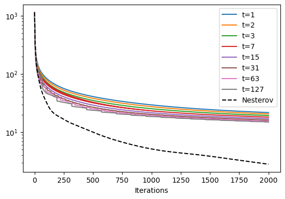
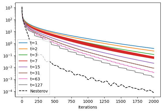
Figure 1: Least squares problems minimizing Axb22subscriptsuperscriptnorm𝐴𝑥𝑏22\|Ax-b\|^{2}_{2} (left) and Axb22+x22subscriptsuperscriptnorm𝐴𝑥𝑏22subscriptsuperscriptnorm𝑥22\|Ax-b\|^{2}_{2}+\|x\|^{2}_{2} (right) with i.i.d. normal entries in An×n𝐴superscript𝑛𝑛A\in\mathbb{R}^{n\times n} and bn𝑏superscript𝑛b\in\mathbb{R}^{n} for n=4000𝑛4000n=4000. Objective gaps are plotted over T=2000𝑇2000T=2000 iterations with h=(1)1h=(1) and with each pattern from Table 1. Note this second objective is substantially more strongly convex, so its faster linear convergence is expected. For comparison, Nesterov’s accelerated method (without modification to utilize strong convexity) is shown.

For strongly convex optimization (or, more generally, any problem satisfying a Hölder growth bound), the classic convergence rates for constant stepsize gradient descent are known to improve. We show the same improvements occur for any straightforward stepsize pattern (see Theorem 2.2) with an additional gain of avg(h)avg\mathrm{avg}(h). We validate that the convergence speed-ups of Table 1 actually occur on randomly generated least squares problems in Figure 1, seeing gains proportional to avg(h)avg\mathrm{avg}(h). These plots also showcase that descent is not ensured within the execution of a straightforward pattern as t=7𝑡7t=7 rapidly oscillates within each pattern while converging overall. Note, gradient descent is not an optimal first-order method as accelerated methods can attain a faster O(1/T2)𝑂1superscript𝑇2O(1/T^{2}) rate. A basic implementation of Nesterov’s accelerated method is included in our numerics to showcase the degree of progress in closing this gap able to be accomplished via our longer steps.

Cyclic, periodically long stepsizes have been used in neural network training schedules [30, 31, 32]. Our results only apply to convex, deterministic problems. New techniques handling nonconvexity and stochasticity would need to be developed to describe the effect of long steps in such settings of machine learning.

Outline. In the remainder of this section, we informally sketch how our proof technique proceeds. Then Section 2 formally introduces our notion of straightforward stepsize patterns, showing that any such pattern has a guarantee of the form (1.4). Section 3 shows the existence of a solution to a certain semidefinite program implies straightforwardness. Section 4 concludes by outlining several future directions of interest enabled by and hopefully able to improve on this work.

1.1 Sketch of Proof Technique - Reducing proving eventual descent to an SDP

Our analysis works by guaranteeing a sufficient decrease is achieved after applying the whole pattern h=(h0,h1,,ht1)subscript0subscript1subscript𝑡1h=(h_{0},h_{1},\dots,h_{t-1}) of t𝑡t steps (but not necessarily descending at any of the intermediate iterates). Our notion of straightforward stepsize patterns aims to ensure that for all δ>0𝛿0\delta>0 small enough, if f(x0)f(x)δ𝑓subscript𝑥0𝑓subscript𝑥𝛿f(x_{0})-f(x_{\star})\leq\delta, then xtsubscript𝑥𝑡x_{t} will always attain a descent of at least

f(xt)f(x)δi=0t1hiLD2δ2.𝑓subscript𝑥𝑡𝑓subscript𝑥𝛿superscriptsubscript𝑖0𝑡1subscript𝑖𝐿superscript𝐷2superscript𝛿2f(x_{t})-f(x_{\star})\leq\delta-\frac{\sum_{i=0}^{t-1}h_{i}}{LD^{2}}\delta^{2}\ . (1.5)

For constant stepsizes equal to one, this amounts to f(x0f(x0)/L)f(x0)δ2/LD2𝑓subscript𝑥0𝑓subscript𝑥0𝐿𝑓subscript𝑥0superscript𝛿2𝐿superscript𝐷2f(x_{0}-\nabla f(x_{0})/L)\leq f(x_{0})-\delta^{2}/LD^{2}, a classic descent result that holds for all L𝐿L-smooth convex f𝑓f.

To prove a descent lemma like (1.5), one can take a direct combination of several known inequalities. This is a well-known approach, equivalent to providing dual solutions to the dual of the associated performance estimation problem. We are given the equalities xk+1=xk(hk/L)f(xk)subscript𝑥𝑘1subscript𝑥𝑘subscript𝑘𝐿𝑓subscript𝑥𝑘x_{k+1}=x_{k}-(h_{k}/L)\nabla f(x_{k}) and f(x)=0𝑓subscript𝑥0\nabla f(x_{\star})=0 and as inequalities an initial distance bound

x0x22D2,subscriptsuperscriptnormsubscript𝑥0subscript𝑥22superscript𝐷2\|x_{0}-x_{\star}\|^{2}_{2}\leq D^{2}\ ,

an initial objective gap bound

f(x0)f(x)δ,𝑓subscript𝑥0𝑓subscript𝑥𝛿f(x_{0})-f(x_{\star})\leq\delta\ ,

and for any xisubscript𝑥𝑖x_{i} and xjsubscript𝑥𝑗x_{j} with i,j{,0,1,2,t}𝑖𝑗012𝑡i,j\in\{\star,0,1,2,\dots t\}, convexity and smoothness imply[33, (2.1.10)]

f(xi)f(xj)+f(xj)T(xixj)+12Lf(xi)f(xj)22.𝑓subscript𝑥𝑖𝑓subscript𝑥𝑗𝑓superscriptsubscript𝑥𝑗𝑇subscript𝑥𝑖subscript𝑥𝑗12𝐿subscriptsuperscriptnorm𝑓subscript𝑥𝑖𝑓subscript𝑥𝑗22f(x_{i})\geq f(x_{j})+\nabla f(x_{j})^{T}(x_{i}-x_{j})+\frac{1}{2L}\|\nabla f(x_{i})-\nabla f(x_{j})\|^{2}_{2}\ .

For any nonnegative multipliers v(δ),w(δ),λi,j(δ)0𝑣𝛿𝑤𝛿subscript𝜆𝑖𝑗𝛿0v(\delta),w(\delta),\lambda_{i,j}(\delta)\geq 0 (parameterized by the initial objective gap δ𝛿\delta), one can combine these inequalities to conclude that on every L𝐿L-smooth convex function, gradient descent (1.3) with stepsizes hh satisfies

v(δ)𝑣𝛿\displaystyle v(\delta) (x0x22D2)subscriptsuperscriptnormsubscript𝑥0subscript𝑥22superscript𝐷2\displaystyle(\|x_{0}-x_{\star}\|^{2}_{2}-D^{2}) (1.6)
+w(δ)𝑤𝛿\displaystyle+w(\delta) (f(x0)f(x)δ)𝑓subscript𝑥0𝑓subscript𝑥𝛿\displaystyle(f(x_{0})-f(x_{\star})-\delta)
+i,j{,0,t}λi,j(δ)subscript𝑖𝑗0𝑡subscript𝜆𝑖𝑗𝛿\displaystyle+\sum_{i,j\in\{\star,0,\dots t\}}\lambda_{i,j}(\delta) (f(xj)+f(xj)T(xixj)+12Lf(xi)f(xj)22f(xi))0.𝑓subscript𝑥𝑗𝑓superscriptsubscript𝑥𝑗𝑇subscript𝑥𝑖subscript𝑥𝑗12𝐿subscriptsuperscriptnorm𝑓subscript𝑥𝑖𝑓subscript𝑥𝑗22𝑓subscript𝑥𝑖0\displaystyle\left(f(x_{j})+\nabla f(x_{j})^{T}(x_{i}-x_{j})+\frac{1}{2L}\|\nabla f(x_{i})-\nabla f(x_{j})\|^{2}_{2}-f(x_{i})\right)\leq 0\ .

Our proof then proceeds by showing carefully selected functions w(δ),v(δ),λ(δ)𝑤𝛿𝑣𝛿𝜆𝛿w(\delta),v(\delta),\lambda(\delta) reduce this inequality to guaranteeing (1.5). We find to prove our guarantees in Table 1, it suffices to set v(δ)=i=0t1hiLD4δ2𝑣𝛿superscriptsubscript𝑖0𝑡1subscript𝑖𝐿superscript𝐷4superscript𝛿2v(\delta)=\frac{\sum_{i=0}^{t-1}h_{i}}{LD^{4}}\delta^{2}, w(δ)=12i=0t1hiLD2δ𝑤𝛿12superscriptsubscript𝑖0𝑡1subscript𝑖𝐿superscript𝐷2𝛿w(\delta)=1-\frac{2\sum_{i=0}^{t-1}h_{i}}{LD^{2}}\delta, and use a linear function λ(δ)=λ+δγ𝜆𝛿𝜆𝛿𝛾\lambda(\delta)=\lambda+\delta\gamma. For this choice of v(δ)𝑣𝛿v(\delta) and w(δ)𝑤𝛿w(\delta), our Theorem 3.1 shows (1.6) implies (1.5) if (λ,γ)𝜆𝛾(\lambda,\gamma) is feasible to a certain SDP. Hence, proving a t𝑡t iteration descent lemma of the form (1.5) can be done by semidefinite programming. Our Theorem 2.1 then completes the argument by showing such a periodic descent guarantee implies the guarantee (1.4).

2 Straightforward Stepsize Patterns

To analyze a given stepsize pattern, we first aim to understand its worst-case problem instance. We do so through the “Performance-Estimation Problem” (PEP) framework of [1]. Given a pattern hh and bounds on smoothness L𝐿L, initial distance to optimal D𝐷D, and initial objective gap δ𝛿\delta, the worst final objective gap able to be produced by one application of the stepsize pattern is given by

pL,D(δ):={maxx0,x,ff(xt)f(x)s.t.f is convex, L-smoothx0x2Df(x0)f(x)δf(x)=0xk+1=xkhkLf(xk)k=0,,t1.assignsubscript𝑝𝐿𝐷𝛿casessubscriptsubscript𝑥0subscript𝑥𝑓𝑓subscript𝑥𝑡𝑓subscript𝑥formulae-sequencest𝑓 is convex, 𝐿-smoothotherwisesubscriptnormsubscript𝑥0subscript𝑥2𝐷otherwise𝑓subscript𝑥0𝑓subscript𝑥𝛿otherwise𝑓subscript𝑥0otherwiseformulae-sequencesubscript𝑥𝑘1subscript𝑥𝑘subscript𝑘𝐿𝑓subscript𝑥𝑘for-all𝑘0𝑡1p_{L,D}(\delta):=\begin{cases}\max_{x_{0},x_{\star},f}&f(x_{t})-f(x_{\star})\\ \mathrm{s.t.}&f\text{ is convex, }L\text{-smooth}\\ &\|x_{0}-x_{\star}\|_{2}\leq D\\ &f(x_{0})-f(x_{\star})\leq\delta\\ &\nabla f(x_{\star})=0\\ &x_{k+1}=x_{k}-\frac{h_{k}}{L}\nabla f(x_{k})\quad\forall k=0,\dots,t-1\ .\end{cases} (2.1)

Note this problem is infinite-dimensional as it optimizes over functions f:n:𝑓superscript𝑛f\colon\mathbb{R}^{n}\rightarrow\mathbb{R} and vectors x0,xnsubscript𝑥0subscript𝑥superscript𝑛x_{0},x_{\star}\in\mathbb{R}^{n} for some given problem dimension n𝑛n. The key insight of Drori and Teboulle [1] is that such infinite-dimensional problems can be relaxed to a finite-dimensional semidefinite program. Subsequently, Taylor et al. [2] showed this relaxation can be made an exact reformulation. We formalize and utilize these insights in Section 3. We note one particular nice property here: pL,Dsubscript𝑝𝐿𝐷p_{L,D} is concave.

Lemma 2.1.

For any L,D>0𝐿𝐷0L,D>0, pL,Dsubscript𝑝𝐿𝐷p_{L,D} is concave.

Proof.

Consider any δ(1),δ(2)superscript𝛿1superscript𝛿2\delta^{(1)},\delta^{(2)}\in\mathbb{R} and λ(0,1)𝜆01\lambda\in(0,1). Denote feasible solutions to the problem defining pL,D(δ(i))subscript𝑝𝐿𝐷superscript𝛿𝑖p_{L,D}(\delta^{(i)}) for each i=1,2𝑖12i=1,2 by f(i),x0(i),x(i)superscript𝑓𝑖subscriptsuperscript𝑥𝑖0subscriptsuperscript𝑥𝑖f^{(i)},x^{(i)}_{0},x^{(i)}_{\star}. Note if no feasible solution exists for either of these problems, one vacuously has concavity as

λpL,D(δ(1))+(1λ)pL,D(δ(2))=pL,D(λδ(1)+(1λ)δ(2)).𝜆subscript𝑝𝐿𝐷superscript𝛿11𝜆subscript𝑝𝐿𝐷superscript𝛿2subscript𝑝𝐿𝐷𝜆superscript𝛿11𝜆superscript𝛿2\lambda p_{L,D}(\delta^{(1)})+(1-\lambda)p_{L,D}(\delta^{(2)})=-\infty\leq p_{L,D}(\lambda\delta^{(1)}+(1-\lambda)\delta^{(2)})\ .

Note without loss of generality, x(i)=0subscriptsuperscript𝑥𝑖0x^{(i)}_{\star}=0 and f(i)(x(i))=0superscript𝑓𝑖subscriptsuperscript𝑥𝑖0f^{(i)}(x^{(i)}_{\star})=0. Then one can easily check λf(1)+(1λ)f(2),λx0(1)+(1λ)x0(2),λx(1)+(1λ)x(2)𝜆superscript𝑓11𝜆superscript𝑓2𝜆superscriptsubscript𝑥011𝜆superscriptsubscript𝑥02𝜆superscriptsubscript𝑥11𝜆superscriptsubscript𝑥2\lambda f^{(1)}+(1-\lambda)f^{(2)},\lambda x_{0}^{(1)}+(1-\lambda)x_{0}^{(2)},\lambda x_{\star}^{(1)}+(1-\lambda)x_{\star}^{(2)} is feasible to the problem defining pL,D(λδ(1)+(1λ)δ(2))subscript𝑝𝐿𝐷𝜆superscript𝛿11𝜆superscript𝛿2p_{L,D}(\lambda\delta^{(1)}+(1-\lambda)\delta^{(2)}). Consequently, taking the supremum over choices of f(i),x0(i)superscript𝑓𝑖superscriptsubscript𝑥0𝑖f^{(i)},x_{0}^{(i)} gives concavity as

λpL,D(δ(1))+(1λ)pL,D(δ(2))pL,D(λδ(1)+(1λ)δ(2)).𝜆subscript𝑝𝐿𝐷superscript𝛿11𝜆subscript𝑝𝐿𝐷superscript𝛿2subscript𝑝𝐿𝐷𝜆superscript𝛿11𝜆superscript𝛿2\displaystyle\lambda p_{L,D}(\delta^{(1)})+(1-\lambda)p_{L,D}(\delta^{(2)})\leq p_{L,D}(\lambda\delta^{(1)}+(1-\lambda)\delta^{(2)})\ .

Generally, the worst-case functions f𝑓f attaining (2.1) can be nontrivial. To find a tractable family of stepsizes for analysis, we focus on ones where this worst-case behavior is no worse than a simple one-dimensional setting: Consider the one-dimensional (nonsmooth) convex function linearly decreasing from x0subscript𝑥0x_{0} to xsubscript𝑥x_{\star} and constant thereafter. That is, given L,D,δ𝐿𝐷𝛿L,D,\delta, consider the problem instance f(x)=max{δx/D,0}𝑓𝑥𝛿𝑥𝐷0f(x)=\max\{\delta x/D,0\}, x0=Dsubscript𝑥0𝐷x_{0}=D, and x=0subscript𝑥0x_{\star}=0. Provided δ𝛿\delta is small enough (i.e., δLD2/i=0t1hi𝛿𝐿superscript𝐷2superscriptsubscript𝑖0𝑡1subscript𝑖\delta\leq LD^{2}/\sum_{i=0}^{t-1}h_{i}), the gradient descent iteration xk+1=xkhkLf(xk)subscript𝑥𝑘1subscript𝑥𝑘subscript𝑘𝐿𝑓subscript𝑥𝑘x_{k+1}=x_{k}-\frac{h_{k}}{L}\nabla f(x_{k}) has

δt=δ0i=0t1hiLD2δ02subscript𝛿𝑡subscript𝛿0superscriptsubscript𝑖0𝑡1subscript𝑖𝐿superscript𝐷2superscriptsubscript𝛿02\displaystyle\delta_{t}=\delta_{0}-\frac{\sum_{i=0}^{t-1}h_{i}}{LD^{2}}\delta_{0}^{2} (2.2)

where δk=f(xk)f(x)subscript𝛿𝑘𝑓subscript𝑥𝑘𝑓subscript𝑥\delta_{k}=f(x_{k})-f(x_{\star}) denotes the objective gap. In this example, gradient descent spends all t𝑡t iterations moving straight forward in a line along the slope. So the descent achieved is just controlled by the objective’s slope δ0/Dsubscript𝛿0𝐷\delta_{0}/D (squared) and the total length of steps taken i=0t1hi/Lsuperscriptsubscript𝑖0𝑡1subscript𝑖𝐿\sum_{i=0}^{t-1}h_{i}/L.

We say that a stepsize pattern hh is straightforward if its worst-case behavior (over all smooth functions, as defined in (2.1)) is no worse than this one-dimensional piecewise linear setting for δ𝛿\delta small enough. Formally, we say that a stepsize pattern hh of length t𝑡t is straightforward if for some Δ(0,1/2]Δ012\Delta\in(0,1/2],

pL,D(δ)δi=0t1hiLD2δ2δ[0,LD2Δ]formulae-sequencesubscript𝑝𝐿𝐷𝛿𝛿superscriptsubscript𝑖0𝑡1subscript𝑖𝐿superscript𝐷2superscript𝛿2for-all𝛿0𝐿superscript𝐷2Δp_{L,D}(\delta)\leq\delta-\frac{\sum_{i=0}^{t-1}h_{i}}{LD^{2}}\delta^{2}\qquad\forall\delta\in[0,LD^{2}\Delta]

for any L,D>0𝐿𝐷0L,D>0. Our analysis of gradient descent with long steps then proceeds by:
(i) Certifying hh is straightforward (able to be computer automated) see Theorem 3.1,
(ii) Solving a resulting recurrence, showing δTLD2avg(h)T+O(1/T2)subscript𝛿𝑇𝐿superscript𝐷2avg𝑇𝑂1superscript𝑇2\delta_{T}\leq\frac{LD^{2}}{\mathrm{avg}(h)T}+O(1/T^{2}) see Theorem 2.1.
The second step is simpler, so we address it first. Additionally, we show the same factor of guarantee improvement avg(h)avg\mathrm{avg}(h) carries over to more structured domains like strongly convex optimization.

2.1 Convergence Guarantees for Straightforward Stepsize Patterns

Note straightforwardness provides no guarantees on the intermediate objective values at iterations k=1,2,t1𝑘12𝑡1k=1,2,\dots t-1. We show in our theorem below descent at every t𝑡tth iteration. To allow for some numerical flexibility, we say a pattern is ϵitalic-ϵ\epsilon-straightforward if for some Δ(0,1/2]Δ012\Delta\in(0,1/2], all δ[0,LD2Δ]𝛿0𝐿superscript𝐷2Δ\delta\in[0,LD^{2}\Delta] have value function bounded by pL,D(δ)δi=0t1(hiϵ)LD2δ2subscript𝑝𝐿𝐷𝛿𝛿superscriptsubscript𝑖0𝑡1subscript𝑖italic-ϵ𝐿superscript𝐷2superscript𝛿2p_{L,D}(\delta)\leq\delta-\frac{\sum_{i=0}^{t-1}(h_{i}-\epsilon)}{LD^{2}}\delta^{2}.

Theorem 2.1.

Consider any L𝐿L-smooth, convex f𝑓f. If h=(h0,,ht1)subscript0subscript𝑡1h=(h_{0},\dots,h_{t-1}) is ϵitalic-ϵ\epsilon-straightforward with parameter Δ(0,1/2]Δ012\Delta\in(0,1/2], then gradient descent (1.3) has, for any s𝑠s\in\mathbb{N}, after T=st𝑇𝑠𝑡T=st gradient steps

f(xT)f(x){(1i=0t1(hiϵ)Δ)s(f(x0)f(x)) if ss¯LD2(avg(h)ϵ)(Ts¯t)+1Δ if s>s¯𝑓subscript𝑥𝑇𝑓subscript𝑥casessuperscript1superscriptsubscript𝑖0𝑡1subscript𝑖italic-ϵΔ𝑠𝑓subscript𝑥0𝑓subscript𝑥 if 𝑠¯𝑠𝐿superscript𝐷2avgitalic-ϵ𝑇¯𝑠𝑡1Δ if 𝑠¯𝑠f(x_{T})-f(x_{\star})\leq\begin{cases}(1-\sum_{i=0}^{t-1}(h_{i}-\epsilon)\Delta)^{s}(f(x_{0})-f(x_{\star}))&\text{ if }s\leq\bar{s}\\ \dfrac{LD^{2}}{(\mathrm{avg}(h)-\epsilon)(T-\bar{s}t)+\frac{1}{\Delta}}&\text{ if }s>\bar{s}\end{cases} (2.3)

where s¯=log(f(x0)f(x)LD2Δ)log(1i=0t1(hiϵ)Δ)¯𝑠𝑓subscript𝑥0𝑓subscript𝑥𝐿superscript𝐷2Δ1superscriptsubscript𝑖0𝑡1subscript𝑖italic-ϵΔ\bar{s}=\left\lceil\frac{\log\left(\frac{f(x_{0})-f(x_{\star})}{LD^{2}\Delta}\right)}{\log(1-\sum_{i=0}^{t-1}(h_{i}-\epsilon)\Delta)}\right\rceil. In particular, suppressing lower-order terms, this guarantee is

f(xT)f(x)LD2(avg(h)ϵ)T+O(1/T2).𝑓subscript𝑥𝑇𝑓subscript𝑥𝐿superscript𝐷2avgitalic-ϵ𝑇𝑂1superscript𝑇2f(x_{T})-f(x_{\star})\leq\frac{LD^{2}}{(\mathrm{avg}(h)-\epsilon)T}+O(1/T^{2})\ .
Proof.

For any ϵ0italic-ϵ0\epsilon\geq 0, we begin by showing ϵitalic-ϵ\epsilon-straightforwardness implies that for any s𝑠s\in\mathbb{N}, the recurrence relation

δ(s+1)t{δsti=0t1(hiϵ)LD2δst2 if δstLD2Δ(1i=0t1(hiϵ)Δ)δst if δst>LD2Δ.subscript𝛿𝑠1𝑡casessubscript𝛿𝑠𝑡superscriptsubscript𝑖0𝑡1subscript𝑖italic-ϵ𝐿superscript𝐷2superscriptsubscript𝛿𝑠𝑡2 if subscript𝛿𝑠𝑡𝐿superscript𝐷2Δ1superscriptsubscript𝑖0𝑡1subscript𝑖italic-ϵΔsubscript𝛿𝑠𝑡 if subscript𝛿𝑠𝑡𝐿superscript𝐷2Δ\delta_{(s+1)t}\leq\begin{cases}\delta_{st}-\frac{\sum_{i=0}^{t-1}(h_{i}-\epsilon)}{LD^{2}}\delta_{st}^{2}&\text{ if }\delta_{st}\leq LD^{2}\Delta\\ \left(1-\sum_{i=0}^{t-1}(h_{i}-\epsilon)\Delta\right)\delta_{st}&\text{ if }\delta_{st}>LD^{2}\Delta\ .\end{cases} (2.4)

Consider first s=0𝑠0s=0. The first case of (2.4) follows from the definition of straightforwardness as δtpL,D(δ0)δ0i=0t1(hiϵ)LD2δ02subscript𝛿𝑡subscript𝑝𝐿𝐷subscript𝛿0subscript𝛿0superscriptsubscript𝑖0𝑡1subscript𝑖italic-ϵ𝐿superscript𝐷2superscriptsubscript𝛿02\delta_{t}\leq p_{L,D}(\delta_{0})\leq\delta_{0}-\frac{\sum_{i=0}^{t-1}(h_{i}-\epsilon)}{LD^{2}}\delta_{0}^{2}. For the second case of (2.4), first note that pL,D()subscript𝑝𝐿𝐷p_{L,D}(\cdot) is concave by Lemma 2.1. Then since pL,D(0)=0subscript𝑝𝐿𝐷00p_{L,D}(0)=0 and pL,D(LD2Δ)LD2(Δi=0t1(hiϵ)Δ2)subscript𝑝𝐿𝐷𝐿superscript𝐷2Δ𝐿superscript𝐷2Δsuperscriptsubscript𝑖0𝑡1subscript𝑖italic-ϵsuperscriptΔ2p_{L,D}\left(LD^{2}\Delta\right)\leq LD^{2}\left(\Delta-\sum_{i=0}^{t-1}(h_{i}-\epsilon)\Delta^{2}\right), every δ0>LD2Δsubscript𝛿0𝐿superscript𝐷2Δ\delta_{0}>LD^{2}\Delta must have

δtpL,D(δ0)δ0LD2ΔpL,D(LD2Δ)δ0(1i=0t1(hiϵ)Δ).subscript𝛿𝑡subscript𝑝𝐿𝐷subscript𝛿0subscript𝛿0𝐿superscript𝐷2Δsubscript𝑝𝐿𝐷𝐿superscript𝐷2Δsubscript𝛿01superscriptsubscript𝑖0𝑡1subscript𝑖italic-ϵΔ\delta_{t}\leq p_{L,D}(\delta_{0})\leq\frac{\delta_{0}}{LD^{2}\Delta}p_{L,D}\left(LD^{2}\Delta\right)\leq\delta_{0}\left(1-\sum_{i=0}^{t-1}(h_{i}-\epsilon)\Delta\right)\ .

As a result, applying the sequence of steps from the straightforward pattern hh from x0subscript𝑥0x_{0} yields δtδ0subscript𝛿𝑡subscript𝛿0\delta_{t}\leq\delta_{0}. Hence xtxDnormsubscript𝑥𝑡subscript𝑥𝐷\|x_{t}-x_{\star}\|\leq D since xtsubscript𝑥𝑡x_{t} lies in the initial level set {xf(x)f(x0)}conditional-set𝑥𝑓𝑥𝑓subscript𝑥0\{x\mid f(x)\leq f(x_{0})\}. Thus the above reasoning can apply inductively, giving the claimed recurrence.

Next, we show this recurrence implies the claimed convergence guarantee (2.3). Suppose first, δstsubscript𝛿𝑠𝑡\delta_{st} is larger than LD2Δ𝐿superscript𝐷2ΔLD^{2}\Delta. Then applying the pattern hh contracts the objective gap444Interestingly, this contraction factor is independent of L,D𝐿𝐷L,D. As a result, problem conditioning plays a minimal role in this initial phase of convergence. Instead, only hh and the associated straightforwardness parameter ΔΔ\Delta matter., inductively giving δst(1i=0t1(hiϵ)Δ)sδ0subscript𝛿𝑠𝑡superscript1superscriptsubscript𝑖0𝑡1subscript𝑖italic-ϵΔ𝑠subscript𝛿0\delta_{st}\leq(1-\sum_{i=0}^{t-1}(h_{i}-\epsilon)\Delta)^{s}\delta_{0}. After at most s¯¯𝑠\bar{s} executions of the stepsize pattern, one must have δstLD2Δsubscript𝛿𝑠𝑡𝐿superscript𝐷2Δ\delta_{st}\leq LD^{2}\Delta. Afterward, for any s>s¯𝑠¯𝑠s>\bar{s}, the objective gap decreases by at least

δ(s+1)tδsti=0t1(hiϵ)LD2δst2.subscript𝛿𝑠1𝑡subscript𝛿𝑠𝑡superscriptsubscript𝑖0𝑡1subscript𝑖italic-ϵ𝐿superscript𝐷2superscriptsubscript𝛿𝑠𝑡2\delta_{(s+1)t}\leq\delta_{st}-\frac{\sum_{i=0}^{t-1}(h_{i}-\epsilon)}{LD^{2}}\delta_{st}^{2}\ .

Solving this recurrence with the initial condition δs¯tLD2Δsubscript𝛿¯𝑠𝑡𝐿superscript𝐷2Δ\delta_{\bar{s}t}\leq LD^{2}\Delta gives

δstLD2i=0t1(hiϵ)(ss¯)+1Δ.subscript𝛿𝑠𝑡𝐿superscript𝐷2superscriptsubscript𝑖0𝑡1subscript𝑖italic-ϵ𝑠¯𝑠1Δ\displaystyle\delta_{st}\leq\frac{LD^{2}}{\sum_{i=0}^{t-1}(h_{i}-\epsilon)(s-\bar{s})+\frac{1}{\Delta}}\ .

2.2 Faster Convergence for Straightforward Patterns given Growth Bounds

A function f𝑓f is μ𝜇\mu-strongly convex if fμ222f-\frac{\mu}{2}\|\cdot\|^{2}_{2} is convex. This condition is well-known to lead to linear convergence for most first-order methods in smooth optimization. More generally, faster convergence occurs whenever f𝑓f satisfies a Hölder growth or error bound condition. Here we consider settings where all xn𝑥superscript𝑛x\in\mathbb{R}^{n} within the level set f(x)f(x0)𝑓𝑥𝑓subscript𝑥0f(x)\leq f(x_{0}) satisfy

f(x)f(x)μqxx2q.𝑓𝑥𝑓subscript𝑥𝜇𝑞subscriptsuperscriptnorm𝑥subscript𝑥𝑞2f(x)-f(x_{\star})\geq\frac{\mu}{q}\|x-x_{\star}\|^{q}_{2}\ . (2.5)

Strong convexity implies this condition with q=2𝑞2q=2 and leads gradient descent with constant h=(1,1,)11h=(1,1,\dots) to converge at a rate of O((1μ/L)T)𝑂superscript1𝜇𝐿𝑇O((1-\mu/L)^{T}). When q>2𝑞2q>2, improved sublinear guarantees of O((L/μ2/qT)q/(q2))𝑂superscript𝐿superscript𝜇2𝑞𝑇𝑞𝑞2O((L/\mu^{2/q}T)^{q/(q-2)}) follow. Below, we show that any straightforward stepsize pattern enjoys the same convergence improvements, gaining a similar factor of avg(h)avg\mathrm{avg}(h).

Theorem 2.2.

Consider any L𝐿L-smooth, convex objective f𝑓f satisfying (2.5). If h=(h0,,ht1)subscript0subscript𝑡1h=(h_{0},\dots,h_{t-1}) is ϵitalic-ϵ\epsilon-straightforward with parameter Δ(0,1/2]Δ012\Delta\in(0,1/2], then gradient descent (1.3) has, for any T=st𝑇𝑠𝑡T=st

f(xT)f(x)(1min{Δ,μ2L}i=0t1(hiϵ))s(f(x0)f(x))𝑓subscript𝑥𝑇𝑓subscript𝑥superscript1Δ𝜇2𝐿superscriptsubscript𝑖0𝑡1subscript𝑖italic-ϵ𝑠𝑓subscript𝑥0𝑓subscript𝑥f(x_{T})-f(x_{\star})\leq\left(1-\min\left\{\Delta,\ \frac{\mu}{2L}\right\}\sum_{i=0}^{t-1}(h_{i}-\epsilon)\right)^{s}(f(x_{0})-f(x_{\star}))

when q=2𝑞2q=2 and when q>2𝑞2q>2 and s>s¯:=log(f(x0)f(x)μ2/(q2)q2/(q2)(LΔ)q/(q2))log(1i=0t1(hiϵ)Δ)𝑠¯𝑠assign𝑓subscript𝑥0𝑓subscript𝑥superscript𝜇2𝑞2superscript𝑞2𝑞2superscript𝐿Δ𝑞𝑞21superscriptsubscript𝑖0𝑡1subscript𝑖italic-ϵΔs>\bar{s}:=\left\lceil\frac{\log\left(\frac{f(x_{0})-f(x_{\star})\mu^{2/(q-2)}}{q^{2/(q-2)}(L\Delta)^{q/(q-2)}}\right)}{\log(1-\sum_{i=0}^{t-1}(h_{i}-\epsilon)\Delta)}\right\rceil has

f(xT)f(x)q(Lμ2/q(q2)(avg(h)ϵ)((ss¯)t))q/(q2).𝑓subscript𝑥𝑇𝑓subscript𝑥𝑞superscript𝐿superscript𝜇2𝑞𝑞2avgitalic-ϵ𝑠¯𝑠𝑡𝑞𝑞2f(x_{T})-f(x_{\star})\leq q\left(\dfrac{L}{\mu^{2/q}(q-2)(\mathrm{avg}(h)-\epsilon)((s-\bar{s})t)}\right)^{q/(q-2)}\ .
Proof.

Let Dk=sup{xxf(x)f(xk)}subscript𝐷𝑘supremumconditionalnorm𝑥subscript𝑥𝑓𝑥𝑓subscript𝑥𝑘D_{k}=\sup\{\|x-x_{\star}\|\mid f(x)\leq f(x_{k})\} denote the size of each level set visited by gradient descent. The growth bound (2.5) ensures Dk(qμδk)1/qsubscript𝐷𝑘superscript𝑞𝜇subscript𝛿𝑘1𝑞D_{k}\leq(\frac{q}{\mu}\delta_{k})^{1/q}. Then the recurrence (2.4) implies

δ(s+1)t{δstμ2/qi=0t1(hiϵ)Lq2/qδst22/q if δstLDst2Δ(1i=0t1(hiϵ)Δ)δst if δst>LDst2Δ.subscript𝛿𝑠1𝑡casessubscript𝛿𝑠𝑡superscript𝜇2𝑞superscriptsubscript𝑖0𝑡1subscript𝑖italic-ϵ𝐿superscript𝑞2𝑞superscriptsubscript𝛿𝑠𝑡22𝑞 if subscript𝛿𝑠𝑡𝐿subscriptsuperscript𝐷2𝑠𝑡Δ1superscriptsubscript𝑖0𝑡1subscript𝑖italic-ϵΔsubscript𝛿𝑠𝑡 if subscript𝛿𝑠𝑡𝐿superscriptsubscript𝐷𝑠𝑡2Δ\delta_{(s+1)t}\leq\begin{cases}\delta_{st}-\frac{\mu^{2/q}\sum_{i=0}^{t-1}(h_{i}-\epsilon)}{Lq^{2/q}}\delta_{st}^{2-2/q}&\text{ if }\delta_{st}\leq LD^{2}_{st}\Delta\\ \left(1-\sum_{i=0}^{t-1}(h_{i}-\epsilon)\Delta\right)\delta_{st}&\text{ if }\delta_{st}>LD_{st}^{2}\Delta\ .\end{cases}

One can bound this recurrence relation by the maximum of the two cases. If q=2𝑞2q=2, both cases give a contraction and so

δst(1min{Δ,μ2L}i=0t1(hiϵ))sδ0.subscript𝛿𝑠𝑡superscript1Δ𝜇2𝐿superscriptsubscript𝑖0𝑡1subscript𝑖italic-ϵ𝑠subscript𝛿0\delta_{st}\leq\left(1-\min\left\{\Delta,\ \frac{\mu}{2L}\right\}\sum_{i=0}^{t-1}(h_{i}-\epsilon)\right)^{s}\delta_{0}\ .

If q>2𝑞2q>2, one has

δ(s+1)tmax{δstμ2/qi=0t1(hiϵ)Lq2/qδst22/q,(1i=0t1(hiϵ)Δ)δst}.subscript𝛿𝑠1𝑡subscript𝛿𝑠𝑡superscript𝜇2𝑞superscriptsubscript𝑖0𝑡1subscript𝑖italic-ϵ𝐿superscript𝑞2𝑞superscriptsubscript𝛿𝑠𝑡22𝑞1superscriptsubscript𝑖0𝑡1subscript𝑖italic-ϵΔsubscript𝛿𝑠𝑡\delta_{(s+1)t}\leq\max\left\{\delta_{st}-\frac{\mu^{2/q}\sum_{i=0}^{t-1}(h_{i}-\epsilon)}{Lq^{2/q}}\delta_{st}^{2-2/q},\ \left(1-\sum_{i=0}^{t-1}(h_{i}-\epsilon)\Delta\right)\delta_{st}\right\}\ .

Solving this recurrence gives linear convergence until the objective gap is less than (q2/qLΔμ2/q)qq2superscriptsuperscript𝑞2𝑞𝐿Δsuperscript𝜇2𝑞𝑞𝑞2\left(\frac{q^{2/q}L\Delta}{\mu^{2/q}}\right)^{\frac{q}{q-2}} is reached, which must occur by iteration s¯¯𝑠\bar{s}, and then afterwards gives a sublinear convergence rate (for example, see [34, Lemma A.1] for this calculation), giving the claim. ∎

Note that the above bound for the case of q>2𝑞2q>2 is independent of D𝐷D. Asymptotically, this is reasonable as better bounds on distance to optimal are eventually available, namely (qμδk)1/qsuperscript𝑞𝜇subscript𝛿𝑘1𝑞(\frac{q}{\mu}\delta_{k})^{1/q}. One could give a bound depending on D=D0𝐷subscript𝐷0D=D_{0} early onby using the stronger bound Dkmin{(qμδk)1/q,D0}subscript𝐷𝑘superscript𝑞𝜇subscript𝛿𝑘1𝑞subscript𝐷0D_{k}\leq\min\{(\frac{q}{\mu}\delta_{k})^{1/q},D_{0}\}. However, once the gap is small enough for the first term to dominate, the bound will again be independent of D0subscript𝐷0D_{0}.

3 Certificates of Straightforwardness

All that remains is to show how one can certify the straightforwardness of a stepsize pattern. We do this in two steps. First, Section 3.1 shows that pL,D(δ)subscript𝑝𝐿𝐷𝛿p_{L,D}(\delta) is upper bounded by an SDP minimization problem using previously developed PEP techniques. Hence straightforwardness is implied by showing the SDP corresponding to each δ[0,LD2Δ]𝛿0𝐿superscript𝐷2Δ\delta\in[0,LD^{2}\Delta] has a sufficiently good feasible solution. Second, Section 3.2 shows that another semidefinite programming feasibility problem can certify that such an interval of solutions exists.

3.1 The Worst-Case Value Function is Upper Bounded by an SDP

We first reformulate the infinite-dimensional problem (2.1) as a finite-dimensional nonconvex quadratically constrained quadratic problem (see (3.1)), relax that formulation into an SDP (see (3.2)), and then upper bound the SDP by its dual problem (see (3.3)). This process was been developed by [1, 2, 3] and is carried out in our particular setting below.

Step 1: A QCQP reformulation. First, as proposed by Drori and Teboulle [1], one can discretize the infinite-dimensional problem defining pL,D(δ)subscript𝑝𝐿𝐷𝛿p_{L,D}(\delta) over all possible objective values fksubscript𝑓𝑘f_{k} and gradients gksubscript𝑔𝑘g_{k} at the points xksubscript𝑥𝑘x_{k} with kIt:={,0,1,t}𝑘superscriptsubscript𝐼𝑡assign01𝑡k\in I_{t}^{\star}:=\{\star,0,1,\dots t\} as done below. Using the interpolation theorem of Taylor et al. [2], this is an exact reformulation rather than a relaxation, giving

pL,D(δ)={maxx0,f,gftfs.t.fifj+gjT(xixj)+12Lgigj22i,jItx0x22D2f0fδx=0,f=0,g=0xi+1=xihiLgii=0,,t1subscript𝑝𝐿𝐷𝛿casessubscriptsubscript𝑥0𝑓𝑔subscript𝑓𝑡subscript𝑓formulae-sequencestformulae-sequencesubscript𝑓𝑖subscript𝑓𝑗superscriptsubscript𝑔𝑗𝑇subscript𝑥𝑖subscript𝑥𝑗12𝐿subscriptsuperscriptnormsubscript𝑔𝑖subscript𝑔𝑗22for-all𝑖𝑗superscriptsubscript𝐼𝑡otherwisesubscriptsuperscriptnormsubscript𝑥0subscript𝑥22superscript𝐷2otherwisesubscript𝑓0subscript𝑓𝛿otherwiseformulae-sequencesubscript𝑥0formulae-sequencesubscript𝑓0subscript𝑔0otherwiseformulae-sequencesubscript𝑥𝑖1subscript𝑥𝑖subscript𝑖𝐿subscript𝑔𝑖for-all𝑖0𝑡1p_{L,D}(\delta)=\begin{cases}\max_{x_{0},f,g}&f_{t}-f_{\star}\\ \mathrm{s.t.}&f_{i}\geq f_{j}+g_{j}^{T}(x_{i}-x_{j})+\frac{1}{2L}\|g_{i}-g_{j}\|^{2}_{2}\qquad\forall i,j\in I_{t}^{\star}\\ &\|x_{0}-x_{\star}\|^{2}_{2}\leq D^{2}\\ &f_{0}-f_{\star}\leq\delta\\ &x_{\star}=0,f_{\star}=0,g_{\star}=0\\ &x_{i+1}=x_{i}-\frac{h_{i}}{L}g_{i}\qquad\forall i=0,\dots,t-1\end{cases} (3.1)

where, without loss of generality, we have fixed x=0,f=0,g=0formulae-sequencesubscript𝑥0formulae-sequencesubscript𝑓0subscript𝑔0x_{\star}=0,f_{\star}=0,g_{\star}=0.

Step 2: An SDP relaxation. Second, one can relax the nonconvex problem (3.1) to the following SDP as done in [2, 3, 15]. We follow the particular notational choices of [13], which recently considered globally, numerically optimizing gradient descent’s stepsizes with fixed total iterations, defining

H𝐻\displaystyle H :=[x0g0g1gt]d×(t+2),assignabsentdelimited-[]subscript𝑥0delimited-∣∣subscript𝑔0subscript𝑔1delimited-∣∣subscript𝑔𝑡superscript𝑑𝑡2\displaystyle:=[x_{0}\mid g_{0}\mid g_{1}\mid\ldots\mid g_{t}]\in\mathbb{R}^{d\times(t+2)}\ ,
G𝐺\displaystyle G :=HTH𝕊+t+2,assignabsentsuperscript𝐻𝑇𝐻superscriptsubscript𝕊𝑡2\displaystyle:=H^{T}H\in\mathbb{S}_{+}^{t+2}\ ,
F𝐹\displaystyle F :=[f0f1ft]1×(t+1),assignabsentdelimited-[]conditionalsubscript𝑓0delimited-∣∣subscript𝑓1subscript𝑓𝑡superscript1𝑡1\displaystyle:=[f_{0}\mid f_{1}\mid\ldots\mid f_{t}]\in\mathbb{R}^{1\times(t+1)}\ ,

with the following notation for selecting columns and elements of H𝐻H and F𝐹F:

𝐠subscript𝐠\displaystyle\mathbf{g}_{\star} :=0t+2,𝐠i:=ei+2t+2,i[0:t]\displaystyle:=0\in\mathbb{R}^{t+2},\;\mathbf{g}_{i}:=e_{i+2}\in\mathbb{R}^{t+2},\quad i\in[0:t]
𝐱0subscript𝐱0\displaystyle\mathbf{x}_{0} :=e1t+2,𝐱:=0t+2,formulae-sequenceassignabsentsubscript𝑒1superscript𝑡2assignsubscript𝐱0superscript𝑡2\displaystyle:=e_{1}\in\mathbb{R}^{t+2},\;\mathbf{x}_{\star}:=0\in\mathbb{R}^{t+2}\ ,
𝐱isubscript𝐱𝑖\displaystyle\mathbf{x}_{i} :=𝐱01Lj=0i1hj𝐠jt+2,i[1:t]\displaystyle:=\mathbf{x}_{0}-\frac{1}{L}\sum_{j=0}^{i-1}h_{j}\mathbf{g}_{j}\in\mathbb{R}^{t+2},\quad i\in[1:t]
𝐟subscript𝐟\displaystyle\mathbf{f}_{\star} :=0t+1,𝐟i:=ei+1t+1,i[0:t].\displaystyle:=0\in\mathbb{R}^{t+1},\;\mathbf{f}_{i}:=e_{i+1}\in\mathbb{R}^{t+1},\quad i\in[0:t]\ .

This notation ensures xi=H𝐱isubscript𝑥𝑖𝐻subscript𝐱𝑖x_{i}=H\mathbf{x}_{i}, gi=H𝐠isubscript𝑔𝑖𝐻subscript𝐠𝑖g_{i}=H\mathbf{g}_{i}, and fi=F𝐟i.subscript𝑓𝑖𝐹subscript𝐟𝑖f_{i}=F\mathbf{f}_{i}. Furthermore, for i,jIt𝑖𝑗superscriptsubscript𝐼𝑡i,j\in I_{t}^{\star}, define

Ai,j(h)subscript𝐴𝑖𝑗\displaystyle A_{i,j}(h) :=𝐠j(𝐱i𝐱j)𝕊t+2,assignabsentdirect-productsubscript𝐠𝑗subscript𝐱𝑖subscript𝐱𝑗superscript𝕊𝑡2\displaystyle:=\mathbf{g}_{j}\odot(\mathbf{x}_{i}-\mathbf{x}_{j})\in\mathbb{S}^{t+2}\ ,
Bi,j(h)subscript𝐵𝑖𝑗\displaystyle B_{i,j}(h) :=(𝐱i𝐱j)(𝐱i𝐱j)𝕊+t+2,assignabsentdirect-productsubscript𝐱𝑖subscript𝐱𝑗subscript𝐱𝑖subscript𝐱𝑗superscriptsubscript𝕊𝑡2\displaystyle:=(\mathbf{x}_{i}-\mathbf{x}_{j})\odot(\mathbf{x}_{i}-\mathbf{x}_{j})\in\mathbb{S}_{+}^{t+2}\ ,
Ci,jsubscript𝐶𝑖𝑗\displaystyle C_{i,j} :=(𝐠i𝐠j)(𝐠i𝐠j)𝕊+t+2,assignabsentdirect-productsubscript𝐠𝑖subscript𝐠𝑗subscript𝐠𝑖subscript𝐠𝑗superscriptsubscript𝕊𝑡2\displaystyle:=(\mathbf{g}_{i}-\mathbf{g}_{j})\odot(\mathbf{g}_{i}-\mathbf{g}_{j})\in\mathbb{S}_{+}^{t+2}\ ,
ai,jsubscript𝑎𝑖𝑗\displaystyle a_{i,j} :=𝐟j𝐟it+1assignabsentsubscript𝐟𝑗subscript𝐟𝑖superscript𝑡1\displaystyle:=\mathbf{f}_{j}-\mathbf{f}_{i}\in\mathbb{R}^{t+1}

where xy=12(xyT+yxT)direct-product𝑥𝑦12𝑥superscript𝑦𝑇𝑦superscript𝑥𝑇x\odot y=\frac{1}{2}(xy^{T}+yx^{T}) denotes the symmetric outer product. This notation is defined so that gjT(xixj)=TrGAi,j(h)superscriptsubscript𝑔𝑗𝑇subscript𝑥𝑖subscript𝑥𝑗Tr𝐺subscript𝐴𝑖𝑗g_{j}^{T}(x_{i}-x_{j})=\mathrm{Tr}GA_{i,j}(h), xixj22=TrGBi,j(h)subscriptsuperscriptnormsubscript𝑥𝑖subscript𝑥𝑗22Tr𝐺subscript𝐵𝑖𝑗\|x_{i}-x_{j}\|^{2}_{2}=\mathrm{Tr}GB_{i,j}(h), and gigj22=TrGCi,jsubscriptsuperscriptnormsubscript𝑔𝑖subscript𝑔𝑗22Tr𝐺subscript𝐶𝑖𝑗\|g_{i}-g_{j}\|^{2}_{2}=\mathrm{Tr}GC_{i,j} for any i,jIt𝑖𝑗superscriptsubscript𝐼𝑡i,j\in I_{t}^{\star}. Then the QCQP formulation (3.1) can be relaxed to

pL,D(δ)subscript𝑝𝐿𝐷𝛿absent\displaystyle p_{L,D}(\delta)\leq {maxF,GF𝐟ts.t.Fai,j+TrGAi,j(h)+12LTrGCi,j0,i,jIt:ijG0TrGB0,D2F𝐟0δ.casessubscript𝐹𝐺𝐹subscript𝐟𝑡s.t.:formulae-sequence𝐹subscript𝑎𝑖𝑗Tr𝐺subscript𝐴𝑖𝑗12𝐿Tr𝐺subscript𝐶𝑖𝑗0for-all𝑖𝑗superscriptsubscript𝐼𝑡𝑖𝑗otherwiseprecedes-or-equals𝐺0otherwiseTr𝐺subscript𝐵0superscript𝐷2otherwise𝐹subscript𝐟0𝛿\displaystyle\begin{cases}\max_{F,G}&F\mathbf{f}_{t}\\ \textrm{s.t.}&Fa_{i,j}+\mathrm{Tr}GA_{i,j}(h)+\frac{1}{2L}\mathrm{Tr}GC_{i,j}\leq 0,\quad\forall i,j\in I_{t}^{\star}:i\neq j\\ &-G\preceq 0\\ &\mathrm{Tr}GB_{0,\star}\leq D^{2}\\ &F\mathbf{f}_{0}\leq\delta\ .\end{cases} (3.2)

Equality holds above if one adds the constraint that rankGnrank𝐺𝑛\mathrm{rank\ }G\leq n where n𝑛n is the dimension of problem instances considered when defining pL,Dsubscript𝑝𝐿𝐷p_{L,D}. This constraint is vacuously true if the considered problem dimension n𝑛n exceeds t+2𝑡2t+2. Consequently, the QCQP (3.1) and the SDP (3.2) are equivalent, provided one allows sufficiently high-dimensional objectives, but may differ if one restricts to finding the worst-case over lower-dimensional problem instances. However, this equality is not needed for our analysis, so we make no such assumption.

Step 3: The upper bounding dual SDP. Third, note the maximization SDP (3.2) is bounded above by its dual minimization SDP by weak duality, giving

pL,D(δ){minλ,v,w,ZD2v+δws.t.i,jIt:ijλi,jai,j=a,twa,0vB0,+i,jIt:ijλi,j(Ai,j(h)+12LCi,j)=ZZ0v,w0,λi,j0,i,jIt:ij.p_{L,D}(\delta)\leq\begin{cases}\min_{\lambda,v,w,Z}&D^{2}v+\delta w\\ \textrm{s.t.}&\sum_{i,j\in I_{t}^{\star}:i\neq j}\lambda_{i,j}a_{i,j}=a_{\star,t}-wa_{\star,0}\\ &vB_{0,\star}+\sum_{i,j\in I_{t}^{\star}:i\neq j}\lambda_{i,j}\left(A_{i,j}(h)+\frac{1}{2L}C_{i,j}\right)=Z\\ &Z\succeq 0\\ &v,w\geq 0,\;\lambda_{i,j}\geq 0,\quad\forall i,j\in I_{t}^{\star}:i\neq j\ .\end{cases} (3.3)

Although it is not needed for our analysis, equality holds here as well (i.e., strong duality holds) due to [2, Theorem 6].

3.2 An SDP Feasibility Certificate that implies Straightforwardness

The preceding bound (3.3) establishes that ϵ0italic-ϵ0\epsilon\geq 0-straightforwardness holds if for some Δ(0,1/2]Δ012\Delta\in(0,1/2], every δ[0,LD2Δ]𝛿0𝐿superscript𝐷2Δ\delta\in[0,LD^{2}\Delta] has a corresponding dual feasible solution with objective at most δi=0t1(hiϵ)LD2δ2𝛿superscriptsubscript𝑖0𝑡1subscript𝑖italic-ϵ𝐿superscript𝐷2superscript𝛿2\delta-\frac{\sum_{i=0}^{t-1}(h_{i}-\epsilon)}{LD^{2}}\delta^{2}. We claim that it suffices to fix L=1,D=1formulae-sequence𝐿1𝐷1L=1,D=1 without loss of generality. For any L𝐿L-smooth f𝑓f with x0xDnormsubscript𝑥0subscript𝑥𝐷\|x_{0}-x_{\star}\|\leq D, this follows by instead considering minimizing f~(x~)=1LD2f(Dx~)~𝑓~𝑥1𝐿superscript𝐷2𝑓𝐷~𝑥\tilde{f}(\tilde{x})=\frac{1}{LD^{2}}f(D\tilde{x}). One can easily verify f~~𝑓\tilde{f} is 111-smooth, has x~0x~1normsubscript~𝑥0subscript~𝑥1\|\tilde{x}_{0}-\tilde{x}_{\star}\|\leq 1 for x~0=Dx0,x~=Dxformulae-sequencesubscript~𝑥0𝐷subscript𝑥0subscript~𝑥𝐷subscript𝑥\tilde{x}_{0}=Dx_{0},\tilde{x}_{\star}=Dx_{\star}, and gradient descent x~k+1=x~khkf~(xk)subscript~𝑥𝑘1subscript~𝑥𝑘subscript𝑘~𝑓subscript𝑥𝑘\tilde{x}_{k+1}=\tilde{x}_{k}-h_{k}\nabla\tilde{f}(x_{k}) produces exactly the iterates of xk+1=xkhk/Lf(xk)subscript𝑥𝑘1subscript𝑥𝑘subscript𝑘𝐿𝑓subscript𝑥𝑘x_{k+1}=x_{k}-h_{k}/L\nabla f(x_{k}) rescaled by D𝐷D. Hence pL,D(δ)=LD2p1,1(δ/LD2)subscript𝑝𝐿𝐷𝛿𝐿superscript𝐷2subscript𝑝11𝛿𝐿superscript𝐷2p_{L,D}(\delta)=LD^{2}p_{1,1}(\delta/LD^{2}).

We restrict our search for dual certificates bounding p1,1(δ)subscript𝑝11𝛿p_{1,1}(\delta) to a special case, which we numerically observed to hold approximately at the minimizers of (3.3): given δ𝛿\delta, fix v=i=0t1(hi+ϵ)δ2𝑣superscriptsubscript𝑖0𝑡1subscript𝑖italic-ϵsuperscript𝛿2v=\sum_{i=0}^{t-1}(h_{i}+\epsilon)\delta^{2} and w=12i=0t1hiδ𝑤12superscriptsubscript𝑖0𝑡1subscript𝑖𝛿w=1-2\sum_{i=0}^{t-1}h_{i}\delta. Noting this fixed variable setting has v+δw=δi=0t1(hiϵ)δ2𝑣𝛿𝑤𝛿superscriptsubscript𝑖0𝑡1subscript𝑖italic-ϵsuperscript𝛿2v+\delta w=\delta-\sum_{i=0}^{t-1}(h_{i}-\epsilon)\delta^{2}, ϵitalic-ϵ\epsilon-straightforwardness follows if one can show feasible solutions with these fixed values exist.

Given δ𝛿\delta and a selection of λ(t+2)×(t+2)𝜆superscript𝑡2𝑡2\lambda\in\mathbb{R}^{(t+2)\times(t+2)} and fixing v𝑣v as above, we define

Zh,ϵ(λ,δ):=i=0t1(hi+ϵ)δ2B0,+i,jIt:ijλi,j(Ai,j(h)+12Ci,j).assignsubscript𝑍italic-ϵ𝜆𝛿superscriptsubscript𝑖0𝑡1subscript𝑖italic-ϵsuperscript𝛿2subscript𝐵0subscript:𝑖𝑗superscriptsubscript𝐼𝑡𝑖𝑗subscript𝜆𝑖𝑗subscript𝐴𝑖𝑗12subscript𝐶𝑖𝑗\displaystyle Z_{h,\epsilon}(\lambda,\delta):=\sum_{i=0}^{t-1}(h_{i}+\epsilon)\delta^{2}B_{0,\star}+\sum_{i,j\in I_{t}^{\star}:i\neq j}\lambda_{i,j}\left(A_{i,j}(h)+\frac{1}{2}C_{i,j}\right)\ . (3.4)

Observe that Zh,ϵ(λ,δ)subscript𝑍italic-ϵ𝜆𝛿Z_{h,\epsilon}(\lambda,\delta) is nearly linear: the first entry has the only nonlinear behavior, depending quadratically on δ𝛿\delta, with the rest depending only linearly on λ𝜆\lambda. Written in block form, we denote

Zh,ϵ(λ,δ)=:[i=0t1(hi+ϵ)δ2mh(λ)Tmh(λ)Mh(λ)]\displaystyle Z_{h,\epsilon}(\lambda,\delta)=:\begin{bmatrix}\sum_{i=0}^{t-1}(h_{i}+\epsilon)\delta^{2}&m_{h}(\lambda)^{T}\\ m_{h}(\lambda)&M_{h}(\lambda)\end{bmatrix} (3.5)

where mh:(t+2)×(t+2)t+1:subscript𝑚superscript𝑡2𝑡2superscript𝑡1m_{h}\colon\mathbb{R}^{(t+2)\times(t+2)}\rightarrow\mathbb{R}^{t+1} and Mh:(t+2)×(t+2)(t+1)×(t+1):subscript𝑀superscript𝑡2𝑡2superscript𝑡1𝑡1M_{h}\colon\mathbb{R}^{(t+2)\times(t+2)}\rightarrow\mathbb{R}^{(t+1)\times(t+1)} are linear functions. Certifying p1,1(δ)δi=0t1(hiϵ)δ2subscript𝑝11𝛿𝛿superscriptsubscript𝑖0𝑡1subscript𝑖italic-ϵsuperscript𝛿2p_{1,1}(\delta)\leq\delta-\sum_{i=0}^{t-1}(h_{i}-\epsilon)\delta^{2} for fixed δ𝛿\delta then follows by showing the following spectral set is nonempty

h,ϵ,δ={λ(t+2)×(t+2)i,jIt:ijλi,jai,j=a,t(12i=0t1hiδ)a,0λ0Zh,ϵ(λ,δ)0}.\displaystyle\mathcal{R}_{h,\epsilon,\delta}=\left\{\lambda\in\mathbb{R}^{(t+2)\times(t+2)}\mid\begin{array}[]{l}\sum_{i,j\in I_{t}^{\star}:i\neq j}\lambda_{i,j}a_{i,j}=a_{\star,t}-\left(1-2\sum_{i=0}^{t-1}h_{i}\delta\right)a_{\star,0}\\ \lambda\geq 0\\ Z_{h,\epsilon}(\lambda,\delta)\succeq 0\end{array}\right\}\ . (3.9)
Lemma 3.1.

A stepsize pattern htsuperscript𝑡h\in\mathbb{R}^{t} is ϵ0italic-ϵ0\epsilon\geq 0-straightforward if for some Δ(0,1/2]Δ012\Delta\in(0,1/2], h,ϵ,δsubscriptitalic-ϵ𝛿\mathcal{R}_{h,\epsilon,\delta} is nonempty for all δ[0,Δ]𝛿0Δ\delta\in[0,\Delta]. Straightforwardness of hh is implied by each h,0,δsubscript0𝛿\mathcal{R}_{h,0,\delta} being nonempty.

This lemma alone does not directly enable the computation of a convergence-proof certificate. One would need certificates of feasibility for the infinitely many sets given by each δ[0,Δ]𝛿0Δ\delta\in[0,\Delta]. The following theorem shows that the existence of such solutions can be certified via a single feasible solution to yet another semidefinite program.

Theorem 3.1.

A stepsize pattern htsuperscript𝑡h\in\mathbb{R}^{t} is ϵ0italic-ϵ0\epsilon\geq 0-straightforward if for some Δ(0,1/2]Δ012\Delta\in(0,1/2], 𝒮h,ϵ,Δsubscript𝒮italic-ϵΔ\mathcal{S}_{h,\epsilon,\Delta} is nonempty where

𝒮h,ϵ,Δ={(λ,γ)(t+2)×(t+2)×(t+2)×(t+2)i,jIt:ijλi,jai,j=a,ta,0i,jIt:ijγi,jai,j=2i=0t1hia,0mh(λ)=0λ0,λ+Δγ0[i=0t1(hi+ϵ)mh(γ)Tmh(γ)Mh(λ)]0[i=0t1(hi+ϵ)mh(γ)Tmh(γ)Mh(λ+Δγ)]0}.\mathcal{S}_{h,\epsilon,\Delta}=\left\{(\lambda,\gamma)\in\mathbb{R}^{(t+2)\times(t+2)}\times\mathbb{R}^{(t+2)\times(t+2)}\mid\begin{array}[]{l}\sum_{i,j\in I_{t}^{\star}:i\neq j}\lambda_{i,j}a_{i,j}=a_{\star,t}-a_{\star,0}\\ \sum_{i,j\in I_{t}^{\star}:i\neq j}\gamma_{i,j}a_{i,j}=2\sum_{i=0}^{t-1}h_{i}a_{\star,0}\\ m_{h}(\lambda)=0\\ \lambda\geq 0,\lambda+\Delta\gamma\geq 0\\ \begin{bmatrix}\sum_{i=0}^{t-1}(h_{i}+\epsilon)&m_{h}(\gamma)^{T}\\ m_{h}(\gamma)&M_{h}(\lambda)\end{bmatrix}\succeq 0\\ \begin{bmatrix}\sum_{i=0}^{t-1}(h_{i}+\epsilon)&m_{h}(\gamma)^{T}\\ m_{h}(\gamma)&M_{h}(\lambda+\Delta\gamma)\end{bmatrix}\succeq 0\end{array}\right\}\ .
Proof.

Let (λ,γ)𝒮h,ϵ,Δ𝜆𝛾subscript𝒮italic-ϵΔ(\lambda,\gamma)\in\mathcal{S}_{h,\epsilon,\Delta}. We prove this by showing λ(δ):=λ+δγh,ϵ,δassignsuperscript𝜆𝛿𝜆𝛿𝛾subscriptitalic-ϵ𝛿\lambda^{(\delta)}:=\lambda+\delta\gamma\in\mathcal{R}_{h,\epsilon,\delta} for every δ[0,Δ]𝛿0Δ\delta\in[0,\Delta] by Lemma 3.1. This amounts to verifying the three conditions defining h,ϵ,δsubscriptitalic-ϵ𝛿\mathcal{R}_{h,\epsilon,\delta} for each λ(δ)superscript𝜆𝛿\lambda^{(\delta)}.

First, we check i,jIt:ijλi,j(δ)ai,j=a,t(12i=0t1hiδ)a,0subscript:𝑖𝑗superscriptsubscript𝐼𝑡𝑖𝑗subscriptsuperscript𝜆𝛿𝑖𝑗subscript𝑎𝑖𝑗subscript𝑎𝑡12superscriptsubscript𝑖0𝑡1subscript𝑖𝛿subscript𝑎0\sum_{i,j\in I_{t}^{\star}:i\neq j}\lambda^{(\delta)}_{i,j}a_{i,j}=a_{\star,t}-\left(1-2\sum_{i=0}^{t-1}h_{i}\delta\right)a_{\star,0}. The first equality defining 𝒮h,ϵ,Δsubscript𝒮italic-ϵΔ\mathcal{S}_{h,\epsilon,\Delta} ensures this for λ(0)=λsuperscript𝜆0𝜆\lambda^{(0)}=\lambda. Adding δ𝛿\delta times the second equality defining 𝒮h,ϵ,Δsubscript𝒮italic-ϵΔ\mathcal{S}_{h,\epsilon,\Delta} establishes the equality for every λ(δ)superscript𝜆𝛿\lambda^{(\delta)} as i,jIt:ij(λi,j(δ)+δγi,j)ai,j=a,t(12i=0t1hiδ)a,0subscript:𝑖𝑗superscriptsubscript𝐼𝑡𝑖𝑗subscriptsuperscript𝜆𝛿𝑖𝑗𝛿subscript𝛾𝑖𝑗subscript𝑎𝑖𝑗subscript𝑎𝑡12superscriptsubscript𝑖0𝑡1subscript𝑖𝛿subscript𝑎0\sum_{i,j\in I_{t}^{\star}:i\neq j}(\lambda^{(\delta)}_{i,j}+\delta\gamma_{i,j})a_{i,j}=a_{\star,t}-\left(1-2\sum_{i=0}^{t-1}h_{i}\delta\right)a_{\star,0}. Second, we check nonnegativity λ(δ)0superscript𝜆𝛿0\lambda^{(\delta)}\geq 0. This follows by noting λ(δ)superscript𝜆𝛿\lambda^{(\delta)} is a convex combination of λ𝜆\lambda and λ+Δγ𝜆Δ𝛾\lambda+\Delta\gamma, which are nonnegative by construction. Finally, we check the nonlinear (but nearly linear) condition Zh,ϵ(λ(δ),δ)0succeeds-or-equalssubscript𝑍italic-ϵsuperscript𝜆𝛿𝛿0Z_{h,\epsilon}(\lambda^{(\delta)},\delta)\succeq 0. We consider the block-form (3.5) of this semidefinite inequality, seeking

Zh,ϵ(λ(δ),δ)=[i=0t1(hi+ϵ)δ2mh(λ(δ))Tmh(λ(δ)))Mh(λ(δ))]0.Z_{h,\epsilon}(\lambda^{(\delta)},\delta)=\begin{bmatrix}\sum_{i=0}^{t-1}(h_{i}+\epsilon)\delta^{2}&m_{h}(\lambda^{(\delta)})^{T}\\ m_{h}(\lambda^{(\delta)}))&M_{h}(\lambda^{(\delta)})\end{bmatrix}\succeq 0\ .

Since mh(λ)=0subscript𝑚𝜆0m_{h}(\lambda)=0, using the linearity of mhsubscript𝑚m_{h} and Mhsubscript𝑀M_{h}, the above can be expanded to equal

[i=0t1(hi+ϵ)δ2δmh(γ)Tδmh(γ)Mh(λ)+δMh(γ)]0.succeeds-or-equalsmatrixsuperscriptsubscript𝑖0𝑡1subscript𝑖italic-ϵsuperscript𝛿2𝛿subscript𝑚superscript𝛾𝑇𝛿subscript𝑚𝛾subscript𝑀𝜆𝛿subscript𝑀𝛾0\begin{bmatrix}\sum_{i=0}^{t-1}(h_{i}+\epsilon)\delta^{2}&\delta m_{h}(\gamma)^{T}\\ \delta m_{h}(\gamma)&M_{h}(\lambda)+\delta M_{h}(\gamma)\end{bmatrix}\succeq 0\ .

Rescaling the first row and column by 1/δ1𝛿1/\delta gives an equivalent condition, which is now linear in δ𝛿\delta,

[i=0t1(hi+ϵ)mh(γ)Tmh(γ)Mh(λ)+δMh(γ)]0.succeeds-or-equalsmatrixsuperscriptsubscript𝑖0𝑡1subscript𝑖italic-ϵsubscript𝑚superscript𝛾𝑇subscript𝑚𝛾subscript𝑀𝜆𝛿subscript𝑀𝛾0\begin{bmatrix}\sum_{i=0}^{t-1}(h_{i}+\epsilon)&m_{h}(\gamma)^{T}\\ m_{h}(\gamma)&M_{h}(\lambda)+\delta M_{h}(\gamma)\end{bmatrix}\succeq 0\ .

When δ=0𝛿0\delta=0 or ΔΔ\Delta, this condition is explicitly ensured by the definition of 𝒮h,ϵ,Δsubscript𝒮italic-ϵΔ\mathcal{S}_{h,\epsilon,\Delta}. Then the linearity and convexity of this condition imply it holds for all intermediate λ(δ)superscript𝜆𝛿\lambda^{(\delta)}, completing the proof. ∎

Note computing a member of 𝒮h,ϵ,Δsubscript𝒮italic-ϵΔ\mathcal{S}_{h,\epsilon,\Delta} does not correspond to solving a particular performance estimation problem. Instead, each member provides a “line segment” of solutions to a series of the performance estimation problems pL,D(δ)subscript𝑝𝐿𝐷𝛿p_{L,D}(\delta) for an interval of possible δ𝛿\delta values.

3.3 Certificates of Straightforwardness Proving Guarantees in Table 1

To prove a given pattern hh converges at rate LD2/avg(h)T𝐿superscript𝐷2avg𝑇LD^{2}/\mathrm{avg}(h)T, we only need to show some 𝒮h,0,Δsubscript𝒮0Δ\mathcal{S}_{h,0,\Delta} is nonempty. The most natural path is to provide an exact member of this set. For all of the stepsizes in Table 1, it was relatively easy to find a feasible solution 𝒮h,0,Δsubscript𝒮0Δ\mathcal{S}_{h,0,\Delta} in floating point arithmetic via an interior point method. However, exactly identifying a member of 𝒮h,0,Δsubscript𝒮0Δ\mathcal{S}_{h,0,\Delta} from this can still be hard.

First, we prove the claimed guarantees for the t=2𝑡2t=2 and t=3𝑡3t=3 stepsize patterns of Table 1 by presenting exact members of 𝒮h,0,Δsubscript𝒮0Δ\mathcal{S}_{h,0,\Delta}. Then, to handle larger values of t𝑡t, we present a simple rounding approach able to produce members of 𝒮h,ϵ,Δsubscript𝒮italic-ϵΔ\mathcal{S}_{h,\epsilon,\Delta}, often with ϵitalic-ϵ\epsilon around the accuracy of our SDP solves 109absentsuperscript109\approx 10^{-9}. This approach produced rational-valued certificates proving the rest of the claimed convergence guarantees in Table 1.

The exact rational arithmetic verifying the correctness of all certificates (λ,γ)𝜆𝛾(\lambda,\gamma) was done in Mathematica 13.0.1.0. Note that the entries in these certificates for t7𝑡7t\geq 7 are entirely computer-generated and lack real human insight. As an example for reference, the certificate for t=7𝑡7t=7 is included in the appendix. Larger certificates are impractical to include here. For example, our t=127𝑡127t=127 guarantee is certificate (λ,γ)𝜆𝛾(\lambda,\gamma) has 326403264032640 nonzero entries. Certificates for every pattern in Table 1 and exact verifying computations are available at github.com/bgrimmer/LongStepCertificates.

Theorem 3.2.

For any η(0,3)𝜂03\eta\in(0,3), the stepsize pattern h=(3η,1.5)3𝜂1.5h=(3-\eta,1.5) is straightforward. Hence gradient descent (1.3) alternating between these two stepsizes has every even T𝑇T satisfy

f(xT)f(x)LD2(2.25η/2)×T+O(1/T2).𝑓subscript𝑥𝑇𝑓subscript𝑥𝐿superscript𝐷22.25𝜂2𝑇𝑂1superscript𝑇2f(x_{T})-f(x_{\star})\leq\frac{LD^{2}}{(2.25-\eta/2)\times T}+O(1/T^{2})\ .
Proof.

For any η(0,3)𝜂03\eta\in(0,3), consider the selection of (λ,γ)𝜆𝛾(\lambda,\gamma) given by

λ=[0000001212000120000],γ=[03η6η26η200(6η)2(6η)200000000].formulae-sequence𝜆matrix0000001212000120000𝛾matrix03𝜂6𝜂26𝜂2006𝜂26𝜂200000000\displaystyle\lambda=\begin{bmatrix}0&0&0&0\\ 0&0&\frac{1}{2}&\frac{1}{2}\\ 0&0&0&\frac{1}{2}\\ 0&0&0&0\end{bmatrix}\ ,\qquad\gamma=\begin{bmatrix}0&3-\eta&\frac{6-\eta}{2}&\frac{6-\eta}{2}\\ 0&0&\frac{-(6-\eta)}{2}&\frac{-(6-\eta)}{2}\\ 0&0&0&0\\ 0&0&0&0\end{bmatrix}\ .

It suffices to show for some Δ(0,1/2]Δ012\Delta\in(0,1/2], (λ,γ)𝒮h,0,Δ𝜆𝛾subscript𝒮0Δ(\lambda,\gamma)\in\mathcal{S}_{h,0,\Delta}. One can easily verify the needed equalities and nonnegativities hold for all 0Δ1/(6η)0Δ16𝜂0\leq\Delta\leq 1/(6-\eta). The first positive semidefiniteness condition of (λ,γ)𝒮h,0,Δ𝜆𝛾subscript𝒮0Δ(\lambda,\gamma)\in\mathcal{S}_{h,0,\Delta} amounts to checking every η(0,3)𝜂03\eta\in(0,3) has

[i=0t1(hi+ϵ)mh(γ)Tmh(γ)Mh(λ)]=[92η2(3η)2(6η)4(6η)4(3η)2122η42η4(6η)42η41212(6η)42η41212]0.matrixsuperscriptsubscript𝑖0𝑡1subscript𝑖italic-ϵsubscript𝑚superscript𝛾𝑇subscript𝑚𝛾subscript𝑀𝜆matrix92𝜂23𝜂26𝜂46𝜂43𝜂2122𝜂42𝜂46𝜂42𝜂412126𝜂42𝜂41212succeeds-or-equals0\begin{bmatrix}\sum_{i=0}^{t-1}(h_{i}+\epsilon)&m_{h}(\gamma)^{T}\\ m_{h}(\gamma)&M_{h}(\lambda)\end{bmatrix}=\begin{bmatrix}\frac{9-2\eta}{2}&\frac{-(3-\eta)}{2}&\frac{-(6-\eta)}{4}&\frac{-(6-\eta)}{4}\\ \frac{-(3-\eta)}{2}&\frac{1}{2}&\frac{2-\eta}{4}&\frac{2-\eta}{4}\\ \frac{-(6-\eta)}{4}&\frac{2-\eta}{4}&\frac{1}{2}&\frac{1}{2}\\ \frac{-(6-\eta)}{4}&\frac{2-\eta}{4}&\frac{1}{2}&\frac{1}{2}\end{bmatrix}\succeq 0\ .

Since this convex condition is linear in η𝜂\eta, it suffices to check it at η=0𝜂0\eta=0 and η=3𝜂3\eta=3. Moreover, for any η(0,3)𝜂03\eta\in(0,3), note this matrix has exactly two zero eigenvalues with associated eigenvectors spanning (1/2,1/2,1,0)121210(1/2,1/2,1,0) and (1/2,1/2,0,1)121201(1/2,1/2,0,1). The second positive semidefiniteness condition amounts to checking an update to this matrix of size ΔΔ\Delta remains positive semidefinite, namely [i=0t1(hi+ϵ)mh(γ)Tmh(γ)Mh(λ+Δγ)]matrixsuperscriptsubscript𝑖0𝑡1subscript𝑖italic-ϵsubscript𝑚superscript𝛾𝑇subscript𝑚𝛾subscript𝑀𝜆Δ𝛾\begin{bmatrix}\sum_{i=0}^{t-1}(h_{i}+\epsilon)&m_{h}(\gamma)^{T}\\ m_{h}(\gamma)&M_{h}(\lambda+\Delta\gamma)\end{bmatrix} which equals

[92η2(3η)2(6η)4(6η)4(3η)2122η42η4(6η)42η41212(6η)42η41212]+[00000326η46η406η40006η400]Δmatrix92𝜂23𝜂26𝜂46𝜂43𝜂2122𝜂42𝜂46𝜂42𝜂412126𝜂42𝜂41212matrix00000326𝜂46𝜂406𝜂40006𝜂400Δ\begin{bmatrix}\frac{9-2\eta}{2}&\frac{-(3-\eta)}{2}&\frac{-(6-\eta)}{4}&\frac{-(6-\eta)}{4}\\ \frac{-(3-\eta)}{2}&\frac{1}{2}&\frac{2-\eta}{4}&\frac{2-\eta}{4}\\ \frac{-(6-\eta)}{4}&\frac{2-\eta}{4}&\frac{1}{2}&\frac{1}{2}\\ \frac{-(6-\eta)}{4}&\frac{2-\eta}{4}&\frac{1}{2}&\frac{1}{2}\end{bmatrix}+\begin{bmatrix}0&0&0&0\\ 0&\frac{-3}{2}&\frac{6-\eta}{4}&\frac{6-\eta}{4}\\ 0&\frac{6-\eta}{4}&0&0\\ 0&\frac{6-\eta}{4}&0&0\end{bmatrix}\Delta

must be positive semidefinite. One can check this added matrix term is positive semidefinite on the subspace spanned by (1/2,1/2,1,0)121210(1/2,1/2,1,0) and (1/2,1/2,0,1)121201(1/2,1/2,0,1) (again by checking when η=0𝜂0\eta=0 and η=3𝜂3\eta=3 and then using convexity). As a result, positive semidefiniteness is maintained for ΔΔ\Delta small enough. Exact arithmetic verifying all of these claims are given in the associated Mathematica notebook. Hence (λ,γ)𝒮h,0,Δ𝜆𝛾subscript𝒮0Δ(\lambda,\gamma)\in\mathcal{S}_{h,0,\Delta}, proving the main claim by Theorem 3.1 and the claimed convergence guarantee by Theorem 2.1. ∎

Theorem 3.3.

The stepsize pattern h=(1.5,4.9,1.5)1.54.91.5h=(1.5,4.9,1.5) is straightforward. Hence gradient descent (1.3) cycling through these three stepsizes has every T=3s𝑇3𝑠T=3s satisfy

f(xT)f(x)LD22.63333×T+O(1/T2).𝑓subscript𝑥𝑇𝑓subscript𝑥𝐿superscript𝐷22.63333𝑇𝑂1superscript𝑇2f(x_{T})-f(x_{\star})\leq\frac{LD^{2}}{2.63333...\times T}+O(1/T^{2})\ .
Proof.

This result is certified with Δ=104Δsuperscript104\Delta=10^{-4} by the following exact values for (λ,γ)𝒮h,0,Δ𝜆𝛾subscript𝒮0Δ(\lambda,\gamma)\in\mathcal{S}_{h,0,\Delta} of

λ=[00000001.950.0030.00700.9500.50.500.006000.5100.00400.0130],γ=[00.0057.8253.94974.0203005.2410.55500007.95.31500001.294700000].formulae-sequence𝜆matrix00000001.950.0030.00700.9500.50.500.006000.5100.00400.0130𝛾matrix00.0057.8253.94974.0203005.2410.55500007.95.31500001.294700000\displaystyle\lambda=\begin{bmatrix}0&0&0&0&0\\ 0&0&1.95&0.003&0.007\\ 0&0.95&0&0.5&0.5\\ 0&0.006&0&0&0.51\\ 0&0.004&0&0.013&0\end{bmatrix},\ \gamma=\begin{bmatrix}0&0.005&7.825&3.9497&4.0203\\ 0&0&-5.24&-10.555&0\\ 0&0&0&7.9&-5.315\\ 0&0&0&0&1.2947\\ 0&0&0&0&0\end{bmatrix}.

Based on numerical exploration, we conjecture that patterns of the form (3η,1.5)3𝜂1.5(3-\eta,1.5) are the longest straightforward patterns of length two and (1.5,5η,1.5)1.55𝜂1.5(1.5,5-\eta,1.5) are the longest of length three.

For larger settings t7𝑡7t\geq 7, determining an exact member of 𝒮h,0,Δsubscript𝒮0Δ\mathcal{S}_{h,0,\Delta} proved difficult. So we resort to a fully automated construction of a convergence guarantee certificate by first numerically computing an approximate member of 𝒮h,0,Δsubscript𝒮0Δ\mathcal{S}_{h,0,\Delta} (via an interior point method) and then rounding to a nearby rational-valued exact member of 𝒮h,ϵ,Δsubscript𝒮italic-ϵΔ\mathcal{S}_{h,\epsilon,\Delta} for some small ϵitalic-ϵ\epsilon. In light of our Theorem 2.1, such rounding only weakens the resulting guarantee’s coefficient from avg(h)avg\mathrm{avg}(h) to avg(h)ϵavgitalic-ϵ\mathrm{avg}(h)-\epsilon.

Computer Generation of Convergence Proof Certificates. Given hh and ΔΔ\Delta,
(i) Numerically compute some (λ~,γ~)~𝜆~𝛾(\tilde{\lambda},\tilde{\gamma}) approximately in 𝒮h,0,Δsubscript𝒮0Δ\mathcal{S}_{h,0,\Delta},
(ii) Compute rational (λ^,γ^)^𝜆^𝛾(\hat{\lambda},\hat{\gamma}) near (λ~,γ~)~𝜆~𝛾(\tilde{\lambda},\tilde{\gamma}) exactly satisfying the three needed equalities,
(iii) Check in exact arithmetic nonnegativity and positive definiteness of Mh(λ^)subscript𝑀^𝜆M_{h}(\hat{\lambda}) and Mh(λ^+Δγ^)subscript𝑀^𝜆Δ^𝛾M_{h}(\hat{\lambda}+\Delta\hat{\gamma}),
(iv) If so, (λ^,γ^)𝒮h,ϵ,Δ^𝜆^𝛾subscript𝒮italic-ϵΔ(\hat{\lambda},\hat{\gamma})\in\mathcal{S}_{h,\epsilon,\Delta}, certifying LD2(avg(h)ϵ)T+O(1/T2)𝐿superscript𝐷2avgitalic-ϵ𝑇𝑂1superscript𝑇2\frac{LD^{2}}{(\mathrm{avg}(h)-\epsilon)T}+O(1/T^{2}) convergence, for

ϵ=max{mh(γ^)TMh(λ^)1mh(γ^),mh(γ^)TMh(λ^+Δγ^)1mh(γ^)}tavg(h).italic-ϵsubscript𝑚superscript^𝛾𝑇subscript𝑀superscript^𝜆1subscript𝑚^𝛾subscript𝑚superscript^𝛾𝑇subscript𝑀superscript^𝜆Δ^𝛾1subscript𝑚^𝛾𝑡avg\epsilon=\frac{\max\{m_{h}(\hat{\gamma})^{T}M_{h}(\hat{\lambda})^{-1}m_{h}(\hat{\gamma}),\ m_{h}(\hat{\gamma})^{T}M_{h}(\hat{\lambda}+\Delta\hat{\gamma})^{-1}m_{h}(\hat{\gamma})\}}{t}-\mathrm{avg}(h)\ .

The above value of ϵitalic-ϵ\epsilon is the smallest value with (λ^,γ^)𝒮h,ϵ,Δ^𝜆^𝛾subscript𝒮italic-ϵΔ(\hat{\lambda},\hat{\gamma})\in\mathcal{S}_{h,\epsilon,\Delta}, since by considering their Schur complements, the two needed positive semidefinite conditions hold if and only if

i=0t1(hi+ϵ)mh(γ^)TMh(λ^)1mh(γ^)0 and i=0t1(hi+ϵ)mh(γ^)TMh(λ^+Δγ^)1mh(γ^)0.superscriptsubscript𝑖0𝑡1subscript𝑖italic-ϵsubscript𝑚superscript^𝛾𝑇subscript𝑀superscript^𝜆1subscript𝑚^𝛾0 and superscriptsubscript𝑖0𝑡1subscript𝑖italic-ϵsubscript𝑚superscript^𝛾𝑇subscript𝑀superscript^𝜆Δ^𝛾1subscript𝑚^𝛾0\sum_{i=0}^{t-1}(h_{i}+\epsilon)-m_{h}(\hat{\gamma})^{T}M_{h}(\hat{\lambda})^{-1}m_{h}(\hat{\gamma})\geq 0\ \text{ and }\sum_{i=0}^{t-1}(h_{i}+\epsilon)-m_{h}(\hat{\gamma})^{T}M_{h}(\hat{\lambda}+\Delta\hat{\gamma})^{-1}m_{h}(\hat{\gamma})\geq 0\ .
Theorem 3.4.

The stepsize patterns of lengths t{7,15,31,63,127}𝑡7153163127t\in\{7,15,31,63,127\} in Table 1 are all ϵitalic-ϵ\epsilon-straightforward for ϵ{109,109,1011,103,104}italic-ϵsuperscript109superscript109superscript1011superscript103superscript104\epsilon\in\{10^{-9},10^{-9},10^{-11},10^{-3},10^{-4}\} with Δ{105,106,108,107,108}Δsuperscript105superscript106superscript108superscript107superscript108\Delta\in\{10^{-5},10^{-6},10^{-8},10^{-7},10^{-8}\}. Hence the convergence guarantees claimed in Table 1 hold for each corresponding “long step” gradient descent method.

Proof.

Certificates (λ^,γ^)𝒮h,ϵ,Δ^𝜆^𝛾subscript𝒮italic-ϵΔ(\hat{\lambda},\hat{\gamma})\in\mathcal{S}_{h,\epsilon,\Delta} (produced via the above procedure) with exact arithmetic validation are available at github.com/bgrimmer/LongStepCertificates. ∎

4 Future Directions

Building on existing performance estimation ideas, we have demonstrated an analysis technique capable of proving convergence of gradient descent using nonconstant, long stepsize patterns, which gain in strength as longer patterns are considered. This runs contrary to widely held intuitions regarding constant stepsize selections and the importance of monotone objective decreases. Instead, we show that long-run performance can improve by periodically taking (very) long steps that may increase the objective value in the short term. We accomplish this via computer-generated proof certificates bounding the effect of many steps collectively by providing solutions for a sequence of related performance estimation problems. We conclude by discussing a few possible future improvements on and shortcomings of this technique.

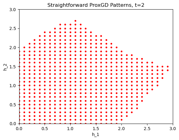
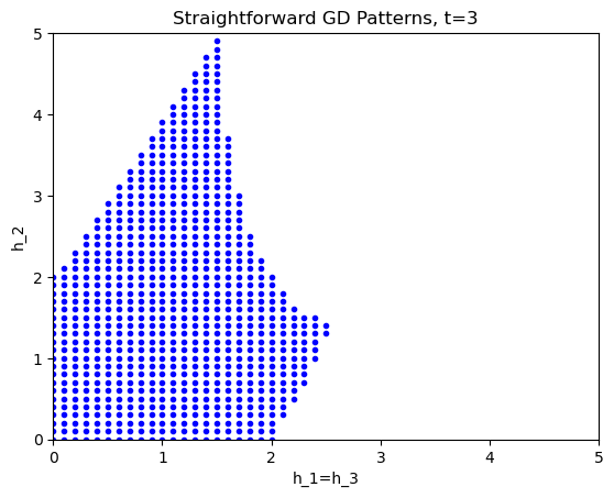
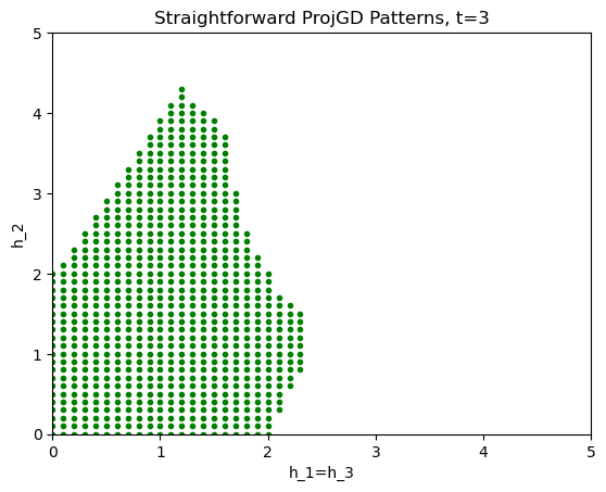
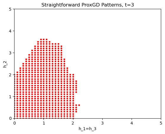
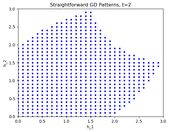
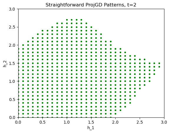
Possible Extension to More Families of Gradient Methods. Often, analysis techniques for gradient descent and its accelerated variants extend rather directly to constrained minimization or minimizing composite objectives f(x)+r(x)𝑓𝑥𝑟𝑥f(x)+r(x) by utilizing projections and proximal operators. PEP techniques naturally extend to these settings. Drori [35, Theorem 2.7 and 2.9] shows the tight convergence rate for projected gradient descent is strictly worse than the unconstrained setting, having rate LD2/4T𝐿superscript𝐷24𝑇LD^{2}/4T instead of (1.2). A similar (small) worsening of the optimal rate also holds for accelerated proximal gradient methods [36]. This difficulty appears to extend to our straightforward analysis technique. Figure 2 shows the length two and three stepsize patterns that numerically satisfy a generalized notion of straightforwardness for gradient descent, projected gradient descent, and proximal gradient descent. The set of “straightforward” patterns for constrained is strictly smaller and composite yet strictly smaller. Consequently, strictly less aggressive stepsizes than Table 1 would be required for future projected or proximal extensions.

The PEP framework has previously been successfully employed in handling settings of inexact gradients [37] and relatively smooth optimization (via Bregman divergences) [7]. Determining the degree to which utilizing periodic long steps can improve the convergence of inexact, Bregman, and stochastic variations of gradient descent also provides interesting future directions.
Refer to caption
Refer to caption
Refer to caption
Refer to caption
Refer to caption
Refer to caption
Figure 2: For unconstrained, constrained, and composite minimization, the stepsize patterns satisfying a natural generalization of straightforwardness are shown. Patterns (h1,h2)subscript1subscript2(h_{1},h_{2}) of length two and symmetric patterns (h1,h2,h1)subscript1subscript2subscript1(h_{1},h_{2},h_{1}) of length three were sampled at every 0.10.10.1 increment. Straightforwardness was approximated by solving a performance estimation problem determining if f(xt)p𝑓subscript𝑥𝑡subscript𝑝f(x_{t})-p_{\star} (or f(xt)+r(xt)p𝑓subscript𝑥𝑡𝑟subscript𝑥𝑡subscript𝑝f(x_{t})+r(x_{t})-p_{\star} for composite problems) is always at most f(x0)phiLD2(f(x0)p)2𝑓subscript𝑥0subscript𝑝subscript𝑖𝐿superscript𝐷2superscript𝑓subscript𝑥0subscript𝑝2f(x_{0})-p_{\star}-\frac{\sum h_{i}}{LD^{2}}(f(x_{0})-p_{\star})^{2} (or f(x0)+r(x0)phiLD2(f(x0)+r(x0)p)2𝑓subscript𝑥0𝑟subscript𝑥0subscript𝑝subscript𝑖𝐿superscript𝐷2superscript𝑓subscript𝑥0𝑟subscript𝑥0subscript𝑝2f(x_{0})+r(x_{0})-p_{\star}-\frac{\sum h_{i}}{LD^{2}}(f(x_{0})+r(x_{0})-p_{\star})^{2}) given the initial gap was at most Δ=104Δsuperscript104\Delta=10^{-4}.

Future Improvements in Algorithm Design. The search for long, straightforward stepsize patterns hh is hard. The patterns presented in Table 1 resulted from substantial brute force searching. The task of maximizing avg(h)avg\mathrm{avg}(h) subject to hh being straightforward, although nonconvex, may be approachable using branch-and-bound techniques similar to those recently developed by Gupta et al. [13] and applied to a range of PEP parameter optimization problems. Such an approach may yield numerically, globally optimal hh for fixed length t𝑡t. This may also generate insights into the general form of the longest straightforward stepsize patterns for each fixed t𝑡t.

One practical drawback of the method (1.3) is the requirement that one knows L𝐿L. Since our analysis in Theorem 2.1 only relies on decreases in objective value after t𝑡t steps, backtracking linesearch schemes or other adaptive ideas may be applicable. For example, one could consider an Armijo-type linesearching procedure, backtracking with an estimate of L~~𝐿\tilde{L} seeking f(xt)f(x0)hiL~f(x0)2𝑓subscript𝑥𝑡𝑓subscript𝑥0subscript𝑖~𝐿superscriptnorm𝑓subscript𝑥02f(x_{t})\leq f(x_{0})-\frac{\sum h_{i}}{\tilde{L}}\|\nabla f(x_{0})\|^{2}. Since convexity ensures f(x0)2δ02/D2superscriptnorm𝑓subscript𝑥02superscriptsubscript𝛿02superscript𝐷2\|\nabla f(x_{0})\|^{2}\geq\delta_{0}^{2}/D^{2}, this condition guarantees the descent required by straightforwardness. Analysis and practical development of such ideas are beyond our scope.

Future Improvements in Analysis Techniques. Future works may improve our analysis by considering other Lyapunov functions. The distance to optimal and norm of the gradient were both used in [4, Chapter 8]. Our proofs are only concerned with the eventual decrease of the objective gap. The analysis of optimal accelerated and subgradient methods relies additionally on the decreasing distance to a minimizer or a decreasing combination thereof. Identifying better Lyapunovs and stepsize patterns guaranteed to eventually decrease them may lead to stronger guarantees.

Future Improvements in Computational Aspects. We observed that numerically computed primal optimal solutions to (3.2) were rank-one for all considered straightforward patterns. This corresponds to the worst-case objective function being essentially one-dimensional. This is in line with many prior PEP-based analyses finding one-dimensional Huber functions often attain the worst-case performance. This property was not used herein but could likely be leveraged to enable customized solvers for evaluating pL,D(δ)subscript𝑝𝐿𝐷𝛿p_{L,D}(\delta) and checking membership of 𝒮h,0,Δsubscript𝒮0Δ\mathcal{S}_{h,0,\Delta}. Such improvements in tractability for SDPs with rank-one solutions have been studied widely [38, 39, 40, 41, 42, 43, 44] and may enable the search for longer, provably faster straightforward stepsize patterns than shown here.

As another avenue of improvement, note that any certificates produced by using floating point arithmetic followed by a rounding step (as done here) will likely lose a small ϵitalic-ϵ\epsilon amount in the guarantee. The use of an algebraic solver, like SPECTRA [45], could enable the automated production of exact certificates of straightforwardness as well as being able to certify when 𝒮h,0,Δsubscript𝒮0Δ\mathcal{S}_{h,0,\Delta} is empty.

Acknowledgements.

The author thanks Jason Altschuler for conversations at the Simons Insitute in Spring 2017 about the preliminary ideas subsequently developed in his excellent Master’s thesis work, Fanghua Chen for preliminary discussions based on numerical observations that motivated this work, and Adrien Taylor and Axel Böhm for providing useful feedback on the initial presentation of this work. The openly released Performance Estimation Problem Branch-and-Bound software of [13] was especially helpful in early explorations and building intuitions.

References

  • [1] Yoel Drori and Marc Teboulle. Performance of first-order methods for smooth convex minimization: a novel approach. Mathematical Programming, 145:451–482, 2012.
  • [2] Adrien Taylor, Julien Hendrickx, and François Glineur. Smooth strongly convex interpolation and exact worst-case performance of first-order methods. Mathematical Programming, 161:307–345, 2017.
  • [3] Adrien Taylor, Julien Hendrickx, and François Glineur. Exact worst-case performance of first-order methods for composite convex optimization. SIAM Journal on Optimization, 27(3):1283–1313, 2017.
  • [4] Jason Altschuler. Greed, hedging, and acceleration in convex optimization. PhD thesis, Massachusetts Institute of Technology, 2018.
  • [5] Etienne de Klerk, François Glineur, and Adrien Taylor. On the worst-case complexity of the gradient method with exact line search for smooth strongly convex functions. Optimization Letters, 11:1185–1199, 2016.
  • [6] Adrien Taylor, Bryan Van Scoy, and Laurent Lessard. Lyapunov functions for first-order methods: Tight automated convergence guarantees. In Proceedings of the 35th International Conference on Machine Learning, volume 80, pages 4897–4906. PMLR, 10–15 Jul 2018.
  • [7] Radu-Alexandru Dragomir, Adrien Taylor, Alexandre d’Aspremont, and Jérôme Bolte. Optimal complexity and certification of bregman first-order methods. Mathematical Programming, 194:41 – 83, 2019.
  • [8] Adrien Taylor and Francis Bach. Stochastic first-order methods: non-asymptotic and computer-aided analyses via potential functions. ArXiv, abs/1902.00947, 2019.
  • [9] Felix Lieder. On the convergence rate of the halpern-iteration. Optimization Letters, pages 1–14, 2020.
  • [10] Ernest Ryu, Adrien Taylor, Carolina Bergeling, and Pontus Giselsson. Operator splitting performance estimation: Tight contraction factors and optimal parameter selection. SIAM Journal on Optimization, 30(3):2251–2271, 2020.
  • [11] Guoyong Gu and Junfeng Yang. Tight sublinear convergence rate of the proximal point algorithm for maximal monotone inclusion problems. SIAM Journal on Optimization, 30(3):1905–1921, 2020.
  • [12] Mathieu Barré, Adrien Taylor, and Francis Bach. Principled analyses and design of first-order methods with inexact proximal operators. Mathematical Programming, 2022.
  • [13] Shuvomoy Das Gupta, Bart P.G. Van Parys, and Ernest Ryu. Branch-and-bound performance estimation programming: A unified methodology for constructing optimal optimization methods. Mathematical Programming, 2023.
  • [14] Donghwan Kim and Jeffrey A. Fessler. Optimized first-order methods for smooth convex minimization. Math. Program., 159(1–2):81–107, sep 2016.
  • [15] Yoel Drori and Adrien Taylor. Efficient first-order methods for convex minimization: a constructive approach. Mathematical Programming, 184:183 – 220, 2018.
  • [16] Donghwan Kim and Jeffrey A. Fessler. Optimizing the efficiency of first-order methods for decreasing the gradient of smooth convex functions. J. Optim. Theory Appl., 188(1):192–219, jan 2021.
  • [17] Donghwan Kim. Accelerated proximal point method for maximally monotone operators. Math. Program., 190(1–2):57–87, nov 2021.
  • [18] Adrien Taylor and Yoel Drori. An optimal gradient method for smooth strongly convex minimization. Math. Program., 199(1–2):557–594, jun 2022.
  • [19] Dimitri P. Bertsekas. Convex optimization algorithms. 2015.
  • [20] Marc Teboulle and Yakov Vaisbourd. An elementary approach to tight worst case complexity analysis of gradient based methods. Math. Program., 201(1–2):63–96, oct 2022.
  • [21] David Young. On richardson’s method for solving linear systems with positive definite matrices. Journal of Mathematics and Physics, 32(1-4):243–255, 1953.
  • [22] Fabian Pedregosa. Acceleration without momentum, 2021.
  • [23] Samet Oymak. Provable super-convergence with a large cyclical learning rate. IEEE Signal Process. Lett., 28:1645–1649, 2021.
  • [24] Antoine Daccache. Performance estimation of the gradient method with fixed arbitrary step sizes. Master’s thesis, Université Catholique de Louvain, 2019.
  • [25] Diego Eloi. Worst-case functions for the gradient method with fixed variable step sizes. Master’s thesis, Université Catholique de Louvain, 2022.
  • [26] V.I. Lebedev and S.A. Finogenov. Ordering of the iterative parameters in the cyclical chebyshev iterative method. USSR Computational Mathematics and Mathematical Physics, 11(2):155–170, 1971.
  • [27] Naman Agarwal, Surbhi Goel, and Cyril Zhang. Acceleration via fractal learning rate schedules. In Proceedings of the 38th International Conference on Machine Learning, volume 139, pages 87–99, 2021.
  • [28] Baptiste Goujaud, Damien Scieur, Aymeric Dieuleveut, Adrien B. Taylor, and Fabian Pedregosa. Super-acceleration with cyclical step-sizes. In Proceedings of The 25th International Conference on Artificial Intelligence and Statistics, pages 3028–3065, 2022.
  • [29] Ching-Pei Lee and Stephen Wright. First-order algorithms converge faster than o(1/k)𝑜1𝑘o(1/k) on convex problems. In Proceedings of the 36th International Conference on Machine Learning, volume 97, pages 3754–3762, 2019.
  • [30] Ilya Loshchilov and Frank Hutter. Sgdr: Stochastic gradient descent with restarts. ArXiv, abs/1608.03983, 2016.
  • [31] Leslie N. Smith. Cyclical learning rates for training neural networks. 2017 IEEE Winter Conference on Applications of Computer Vision (WACV), pages 464–472, 2015.
  • [32] Leslie N. Smith and Nicholay Topin. Super-convergence: very fast training of neural networks using large learning rates. In Defense + Commercial Sensing, 2017.
  • [33] Yurii Nesterov. Introductory Lectures on Convex Optimization: A Basic Course. Springer Publishing Company, Incorporated, 1 edition, 2014.
  • [34] Mateo Díaz and Benjamin Grimmer. Optimal convergence rates for the proximal bundle method. SIAM Journal on Optimization, 33(2):424–454, 2023.
  • [35] Yoel Drori. Contributions to the complexity analysis of optimization algorithms. PhD thesis, Tel-Aviv University, 2014.
  • [36] Uijeong Jang, Shuvomoy Das Gupta, and Ernest K. Ryu. Computer-assisted design of accelerated composite optimization methods: Optista, 2023.
  • [37] Etienne De Klerk, François Glineur, and Adrien B. Taylor. Worst-case convergence analysis of inexact gradient and newton methods through semidefinite programming performance estimation. SIAM Journal on Optimization, 30(3):2053–2082, 2020.
  • [38] Stefania Bellavia, Jacek Gondzio, and Margherita Porcelli. A relaxed interior point method for low-rank semidefinite programming problems with applications to matrix completion. Journal of Scientific Computing, 89, 2019.
  • [39] Lijun Ding, Alp Yurtsever, Volkan Cevher, Joel A. Tropp, and Madeleine Udell. An optimal-storage approach to semidefinite programming using approximate complementarity. SIAM Journal on Optimization, 31(4):2695–2725, 2021.
  • [40] Alp Yurtsever, Joel A. Tropp, Olivier Fercoq, Madeleine Udell, and Volkan Cevher. Scalable semidefinite programming. SIAM Journal on Mathematics of Data Science, 3(1):171–200, 2021.
  • [41] Mario Souto, Joaquim D. Garcia, and Álvaro Veiga. Exploiting low-rank structure in semidefinite programming by approximate operator splitting. Optimization, 71(1):117–144, 2022.
  • [42] Alex L. Wang, Yunlei Lu, and Fatma Kilinç-Karzan. Implicit regularity and linear convergence rates for the generalized trust-region subproblem. SIAM Journal on Optimization, 33(2):1250–1278, 2023.
  • [43] Lijun Ding and Benjamin Grimmer. Revisiting spectral bundle methods: Primal-dual (sub)linear convergence rates. SIAM Journal on Optimization, 33(2):1305–1332, 2023.
  • [44] Alex L. Wang and Fatma Kilinc-Karzan. Accelerated first-order methods for a class of semidefinite programs, 2022.
  • [45] Didier Henrion, Simone Naldi, and Mohab Safey El Din. Spectra – a maple library for solving linear matrix inequalities in exact arithmetic. Optimization Methods and Software, 34:62 – 78, 2016.

Appendix A A Computer-Generated Straightforwardness Certificate with Δ=105Δsuperscript105\Delta=10^{-5} and ϵ=109italic-ϵsuperscript109\epsilon=10^{-9} for h=(1.5,2.2,1.5,12.0,1.5,2.2,1.5)1.52.21.512.01.52.21.5h=(1.5,2.2,1.5,12.0,1.5,2.2,1.5)

Below is a certificate (λ^,γ^)𝒮h,ϵ,Δ^𝜆^𝛾subscript𝒮italic-ϵΔ(\hat{\lambda},\hat{\gamma})\in\mathcal{S}_{h,\epsilon,\Delta}, completely computer generated, proving a LD2/(3.1999999×T)𝐿superscript𝐷23.1999999𝑇LD^{2}/(3.1999999\times T) rate for the pattern of length t=7𝑡7t=7 in Table 1. Given the length of these 9×9999\times 9 matrices, we display their first five and last four columns separately below. Exact calculations verifying the feasibility of these values are given in the associated publicly posted Mathematica notebook.

λ^1:5=[00000008837407518919583450359962737049653706881408023112305843009213693952960254226721649144115188075855872021915229643354572251799813685248041182905385552732251799813685248268840956528327545035996273704960672167833172040123058430092136939524407991053556385180143985094819840580112362698432911258999068426240131368118986041111529215046068469762695784755734549225179981368524880688660105248332251799813685248001137203495150241461168601842738790446889262252128259223372036854775808457297275897709746116860184273879041182579142099203115292150460684697605789750435206701184467440737095516164956986009057139922337203685477580852042470889583454611686018427387904537592724670354592233720368547758080796511593423823336893488147419103232665341869170294992233720368547758084849791056907609461168601842738790472886858194389519223372036854775808019778100933741399223372036854775808122231631113773511529215046068469766194623724653895461168601842738790415040519345775451152921504606846976],subscript^𝜆:15matrix00000008837407518919583450359962737049653706881408023112305843009213693952960254226721649144115188075855872021915229643354572251799813685248041182905385552732251799813685248268840956528327545035996273704960672167833172040123058430092136939524407991053556385180143985094819840580112362698432911258999068426240131368118986041111529215046068469762695784755734549225179981368524880688660105248332251799813685248001137203495150241461168601842738790446889262252128259223372036854775808457297275897709746116860184273879041182579142099203115292150460684697605789750435206701184467440737095516164956986009057139922337203685477580852042470889583454611686018427387904537592724670354592233720368547758080796511593423823336893488147419103232665341869170294992233720368547758084849791056907609461168601842738790472886858194389519223372036854775808019778100933741399223372036854775808122231631113773511529215046068469766194623724653895461168601842738790415040519345775451152921504606846976\hat{\lambda}_{1:5}=\begin{bmatrix}0&0&0&0&0\\ 0&0&\frac{8837407518919583}{4503599627370496}&\frac{5370688140802311}{2305843009213693952}&\frac{960254226721649}{144115188075855872}\\ 0&\frac{2191522964335457}{2251799813685248}&0&\frac{4118290538555273}{2251799813685248}&\frac{2688409565283275}{4503599627370496}\\ 0&\frac{6721678331720401}{2305843009213693952}&\frac{4407991053556385}{18014398509481984}&0&\frac{5801123626984329}{1125899906842624}\\ 0&\frac{1313681189860411}{1152921504606846976}&\frac{2695784755734549}{2251799813685248}&\frac{8068866010524833}{2251799813685248}&0\\ 0&\frac{1137203495150241}{4611686018427387904}&\frac{4688926225212825}{9223372036854775808}&\frac{4572972758977097}{4611686018427387904}&\frac{1182579142099203}{1152921504606846976}\\ 0&\frac{5789750435206701}{18446744073709551616}&\frac{4956986009057139}{9223372036854775808}&\frac{5204247088958345}{4611686018427387904}&\frac{5375927246703545}{9223372036854775808}\\ 0&\frac{7965115934238233}{36893488147419103232}&\frac{6653418691702949}{9223372036854775808}&\frac{4849791056907609}{4611686018427387904}&\frac{7288685819438951}{9223372036854775808}\\ 0&\frac{1977810093374139}{9223372036854775808}&\frac{1222316311137735}{1152921504606846976}&\frac{6194623724653895}{4611686018427387904}&\frac{1504051934577545}{1152921504606846976}\\ \end{bmatrix},
λ^6:9=[00004697224493034383922337203685477580883683942720759532305843009213693952612827862608699392233720368547758088054372350113659936893488147419103232773337087194602546116860184273879045388133457257119230584300921369395281194395504844794611686018427387904197971868574958379223372036854775808274068257324002757646075230342348852903337777407811152921504606846976487738150614220511529215046068469761248592960200977523058430092136939528956652459407733720575940379279364723166920241497180143985094819845356440120675597180143985094819843393190207843073091152921504606846976077284464919982745035996273704962338413531710477288230376151711744133814325576754752305843009213693952692900783119436128823037615171174408173541145090013360287970189639683837009581398546887184467440737095516163923691798295005144115188075855872125043808424772928823037615171174401898568301224761428336893488147419103232130370578063692251799813685248736785953323368957646075230342348828763967105421892882303761517117440],subscript^𝜆:69matrix00004697224493034383922337203685477580883683942720759532305843009213693952612827862608699392233720368547758088054372350113659936893488147419103232773337087194602546116860184273879045388133457257119230584300921369395281194395504844794611686018427387904197971868574958379223372036854775808274068257324002757646075230342348852903337777407811152921504606846976487738150614220511529215046068469761248592960200977523058430092136939528956652459407733720575940379279364723166920241497180143985094819845356440120675597180143985094819843393190207843073091152921504606846976077284464919982745035996273704962338413531710477288230376151711744133814325576754752305843009213693952692900783119436128823037615171174408173541145090013360287970189639683837009581398546887184467440737095516163923691798295005144115188075855872125043808424772928823037615171174401898568301224761428336893488147419103232130370578063692251799813685248736785953323368957646075230342348828763967105421892882303761517117440\hat{\lambda}_{6:9}=\begin{bmatrix}0&0&0&0\\ \frac{4697224493034383}{9223372036854775808}&\frac{8368394272075953}{2305843009213693952}&\frac{6128278626086993}{9223372036854775808}&\frac{80543723501136599}{36893488147419103232}\\ \frac{7733370871946025}{4611686018427387904}&\frac{5388133457257119}{2305843009213693952}&\frac{8119439550484479}{4611686018427387904}&\frac{19797186857495837}{9223372036854775808}\\ \frac{2740682573240027}{576460752303423488}&\frac{5290333777740781}{1152921504606846976}&\frac{4877381506142205}{1152921504606846976}&\frac{12485929602009775}{2305843009213693952}\\ \frac{8956652459407733}{72057594037927936}&\frac{4723166920241497}{18014398509481984}&\frac{5356440120675597}{18014398509481984}&\frac{339319020784307309}{1152921504606846976}\\ 0&\frac{772844649199827}{4503599627370496}&\frac{2338413531710477}{288230376151711744}&\frac{13381432557675475}{2305843009213693952}\\ \frac{6929007831194361}{288230376151711744}&0&\frac{8173541145090013}{36028797018963968}&\frac{3837009581398546887}{18446744073709551616}\\ \frac{3923691798295005}{144115188075855872}&\frac{1250438084247729}{288230376151711744}&0&\frac{18985683012247614283}{36893488147419103232}\\ \frac{13037057806369}{2251799813685248}&\frac{7367859533233689}{576460752303423488}&\frac{2876396710542189}{288230376151711744}&0\\ \end{bmatrix},
γ^1:5=[014450477826654193602879701896396804403953050470099360287970189639681206392980772683714411518807585587231585679433228910031441151880758558720048762141361048311407374883553288833525210676647112589990684262421733428293627432814749767106560345274475575430170368744177664063374930117086773602879701896396861754824480557312251799813685248058651891156720773602879701896396876944642360060672814749767106560576108595312145114411518807585587208990085085489805562949953421312818072422166392390071992547409921706502409602277036874417766400814636363991245225179981368524850023822230448799007199254740992582432428987248745035996273704965420042187723199225179981368524803576868018334213180143985094819843095322656598895180143985094819844741216870166437450359962737049687421076781189271801439850948198407467009600885335720575940379279367502387060304591180143985094819842299019529082251225179981368524852260163911291054503599627370496051714542687839551801439850948198449760896598818554503599627370496849946842273963112589990684262440413780731262392251799813685248],subscript^𝛾:15matrix014450477826654193602879701896396804403953050470099360287970189639681206392980772683714411518807585587231585679433228910031441151880758558720048762141361048311407374883553288833525210676647112589990684262421733428293627432814749767106560345274475575430170368744177664063374930117086773602879701896396861754824480557312251799813685248058651891156720773602879701896396876944642360060672814749767106560576108595312145114411518807585587208990085085489805562949953421312818072422166392390071992547409921706502409602277036874417766400814636363991245225179981368524850023822230448799007199254740992582432428987248745035996273704965420042187723199225179981368524803576868018334213180143985094819843095322656598895180143985094819844741216870166437450359962737049687421076781189271801439850948198407467009600885335720575940379279367502387060304591180143985094819842299019529082251225179981368524852260163911291054503599627370496051714542687839551801439850948198449760896598818554503599627370496849946842273963112589990684262440413780731262392251799813685248\hat{\gamma}_{1:5}=\begin{bmatrix}0&\frac{1445047782665419}{360287970189639680}&\frac{4403953050470099}{36028797018963968}&\frac{12063929807726837}{144115188075855872}&\frac{3158567943322891003}{144115188075855872}\\ 0&0&-\frac{4876214136104831}{140737488355328}&-\frac{8833525210676647}{1125899906842624}&-\frac{2173342829362743}{281474976710656}\\ 0&-\frac{3452744755754301}{70368744177664}&0&-\frac{6337493011708677}{36028797018963968}&-\frac{6175482448055731}{2251799813685248}\\ 0&\frac{5865189115672077}{36028797018963968}&-\frac{7694464236006067}{281474976710656}&0&-\frac{5761085953121451}{144115188075855872}\\ 0&\frac{8990085085489805}{562949953421312}&\frac{8180724221663923}{9007199254740992}&-\frac{170650240960227}{70368744177664}&0\\ 0&\frac{814636363991245}{2251799813685248}&-\frac{5002382223044879}{9007199254740992}&-\frac{5824324289872487}{4503599627370496}&-\frac{5420042187723199}{2251799813685248}\\ 0&\frac{3576868018334213}{18014398509481984}&-\frac{3095322656598895}{18014398509481984}&-\frac{4741216870166437}{4503599627370496}&\frac{8742107678118927}{18014398509481984}\\ 0&\frac{7467009600885335}{72057594037927936}&\frac{7502387060304591}{18014398509481984}&-\frac{2299019529082251}{2251799813685248}&\frac{5226016391129105}{4503599627370496}\\ 0&\frac{5171454268783955}{18014398509481984}&\frac{4976089659881855}{4503599627370496}&-\frac{849946842273963}{1125899906842624}&\frac{4041378073126239}{2251799813685248}\\ \end{bmatrix},
γ^6:9=[8427712788787704752882303761517117441763107326300397405288230376151711744490223898427757151720575940379279362460369054769201053602879701896396875753742647470131125899906842624847735720154307140737488355328364417869530403356294995342131220658178574857592814749767106562568666508774535629499534213122501054473773415112589990684262410082188662074672814749767106566366578400890641225179981368524848191577422531212251799813685248813010563985332318014398509481984201941918877692711258999068426242348470109478957281474976710656451884763914337281474976710656774282369337669518014398509481984290807669822923522517998136852486004115926843261112589990684262403545908575737889288230376151711744308210308568884718014398509481984363184768493823511258999068426246392823462111415720575940379279360226196870745667900719925474099252339388360387392251799813685248345410204791487590071992547409922760923356849777360287970189639680664739622472857225179981368524819574219564881814503599627370496717413743890708745035996273704964503200630060789360287970189639680].subscript^𝛾:69matrix8427712788787704752882303761517117441763107326300397405288230376151711744490223898427757151720575940379279362460369054769201053602879701896396875753742647470131125899906842624847735720154307140737488355328364417869530403356294995342131220658178574857592814749767106562568666508774535629499534213122501054473773415112589990684262410082188662074672814749767106566366578400890641225179981368524848191577422531212251799813685248813010563985332318014398509481984201941918877692711258999068426242348470109478957281474976710656451884763914337281474976710656774282369337669518014398509481984290807669822923522517998136852486004115926843261112589990684262403545908575737889288230376151711744308210308568884718014398509481984363184768493823511258999068426246392823462111415720575940379279360226196870745667900719925474099252339388360387392251799813685248345410204791487590071992547409922760923356849777360287970189639680664739622472857225179981368524819574219564881814503599627370496717413743890708745035996273704964503200630060789360287970189639680\hat{\gamma}_{6:9}=\begin{bmatrix}\frac{842771278878770475}{288230376151711744}&\frac{1763107326300397405}{288230376151711744}&\frac{490223898427757151}{72057594037927936}&\frac{246036905476920105}{36028797018963968}\\ -\frac{7575374264747013}{1125899906842624}&-\frac{847735720154307}{140737488355328}&-\frac{3644178695304033}{562949953421312}&-\frac{2065817857485759}{281474976710656}\\ \frac{256866650877453}{562949953421312}&-\frac{2501054473773415}{1125899906842624}&-\frac{1008218866207467}{281474976710656}&-\frac{6366578400890641}{2251799813685248}\\ \frac{4819157742253121}{2251799813685248}&\frac{8130105639853323}{18014398509481984}&\frac{2019419188776927}{1125899906842624}&\frac{2348470109478957}{281474976710656}\\ \frac{451884763914337}{281474976710656}&\frac{7742823693376695}{18014398509481984}&\frac{2908076698229235}{2251799813685248}&-\frac{6004115926843261}{1125899906842624}\\ 0&-\frac{3545908575737889}{288230376151711744}&\frac{3082103085688847}{18014398509481984}&\frac{3631847684938235}{1125899906842624}\\ -\frac{6392823462111415}{72057594037927936}&0&\frac{226196870745667}{9007199254740992}&-\frac{5233938836038739}{2251799813685248}\\ -\frac{3454102047914875}{9007199254740992}&-\frac{2760923356849777}{36028797018963968}&0&-\frac{664739622472857}{2251799813685248}\\ -\frac{1957421956488181}{4503599627370496}&-\frac{7174137438907087}{4503599627370496}&-\frac{4503200630060789}{36028797018963968}&0\\ \end{bmatrix}.