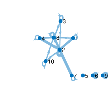
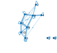
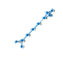
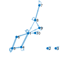
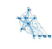
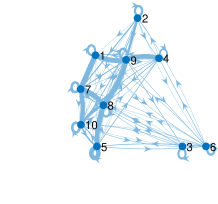
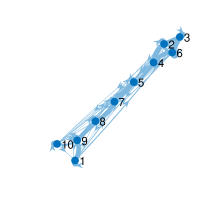
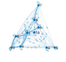
Sparse Graphical Linear Dynamical Systems

\nameEmilie Chouzenoux \emailemilie.chouzenoux@inria.fr
\addrCenter for Visual Computing
Inria, University Paris Saclay
91190 Gif-sur-Yvette, France \AND\nameVíctor Elvira \emailvictor.elvira@ed.ac.uk
\addrSchool of Mathematics
University of Edinburgh
EH9 3FD Edinburgh, UK
Abstract

Time-series datasets are central in numerous fields of science and engineering, such as biomedicine, Earth observation, and network analysis. Extensive research exists on state-space models (SSMs), which are powerful mathematical tools that allow for probabilistic and interpretable learning on time series. Estimating the model parameters in SSMs is arguably one of the most complicated tasks, and the inclusion of prior knowledge is known to both ease the interpretation but also to complicate the inferential tasks. Very recent works have attempted to incorporate a graphical perspective on some of those model parameters, but they present notable limitations that this work addresses. More generally, existing graphical modeling tools are designed to incorporate either static information, focusing on statistical dependencies among independent random variables (e.g., graphical Lasso approach), or dynamic information, emphasizing causal relationships among time series samples (e.g., graphical Granger approaches). However, there are no joint approaches combining static and dynamic graphical modeling within the context of SSMs. This work proposes a novel approach to fill this gap by introducing a joint graphical modeling framework that bridges the static graphical Lasso model and a causal-based graphical approach for the linear-Gaussian SSM. We present DGLASSO (Dynamic Graphical Lasso), a new inference method within this framework that implements an efficient block alternating majorization-minimization algorithm. The algorithm’s convergence is established by departing from modern tools from nonlinear analysis. Experimental validation on synthetic and real weather variability data showcases the effectiveness of the proposed model and inference algorithm. This work will significantly contribute to the understanding and utilization of time-series data in diverse scientific and engineering applications where incorporating a graphical approach is essential to perform the inference.

Keywords: State-space models, graph inference, sparsity, graphical lasso, expectation-maximization, proximal algorithm

1 Introduction

Time series appear in applications of most fields of science and engineering, ranging from biomedicine, Earth observation, or network analysis, to name a few. The literature of time-series analysis in the last century is vast, mostly dominated by auto-regressive moving-averaging (ARMA) models and their extensions (Hamilton, 2020).

With the surge of the Bayesian paradigm, state-space models (SSMs) have became very popular in the last decades (Hamilton, 1994; Kim and Nelson, 1999; Sarkka, 2013) for time series modeling. SSMs characterize complex systems through discrete-time models composed of a hidden (or latent) state that evolves in a Markovian manner. SSMs are composed of a state model, which can mimic realistically the complicated dynamics of the system, and the observation model, which links the temporal observations to the hidden state at the same time step. In SSMs, the Bayesian filtering task consists on computing the posterior probability density function (pdf) of the hidden state at a given time step, given all observations from the time series available up to that time. However, in most SSMs the posterior pdf is intractable and must be approximated, generally through particle filters (Djuric et al., 2003; Doucet et al., 2009; Naesseth et al., 2019). One relevant exception is the linear-Gaussian state-space model (LG-SSM), which allows for exact inference, when the model parameters are known, through the Kalman filter and the Rauch-Tung-Striebel (RTS) smoother (Sarkka, 2013, Chapter 8). The LG-SSM is arguably the most popular model and is still subject of intense research (Sarkka, 2013, Chapter 4). The literature of parameter estimation for LG-SSMs considers both probabilistic and point-wise approaches. The former methods can be applied for a wider class of SSMs (i.e., beyond LG-SSMs) and include for instance particle Markov chain Monte Carlo (Andrieu et al., 2010), sequential Monte Carlo squared (Chopin et al., 2013), and nested particle filters (Crisan and Miguez, 2018; Pérez-Vieites and Míguez, 2021) (see (Kantas et al., 2015) for a review).

One of the main challenges in SSMs is the estimation of the model parameters. In its canonical version, the LG-SSM is composed of four parameters. The state model is parametrized by the so-called transition matrix, which linearly links consecutive states, and the covariance matrix of the additive Gaussian state noise. The observation model is parametrized by the observation matrix, which connects (also linearly) the state with the observation at the same time-step, and the covariance matrix of the additive Gaussian observation noise. Point-wise approaches are generally based on maximum likelihood estimation of the model parameters in LG-SSMs (Sarkka, 2013, Chap. 12). A first family of methods implement recursive schemes to compute first and second derivatives of the likelihood with respect to the unknown parameters (Segal and Weinstein, 1988, 1989; Nagakura, 2021; Gupta and Mehra, 1974) (see the discussion in (Cappe et al., 2005, Sec. 10.2.4)). Iterative optimizers such as quasi-Newton (Olsson et al., 2007) or Newton-Raphson (Gupta and Mehra, 1974) are then employed to get a maximum likelihood estimate. However, due to the intricate form of the likelihood function, these optimization solvers must be used in a black-box setting, which prevents from the implementation of efficient linesearch procedures, and limits considerably the convergence guarantees. The second family of point-wise methods is based on expectation-minimization (EM) algorithms (Shumway and Stoffer, 1982)(Cappe et al., 2005, Sec. 10.4)(Sarkka, 2013, Sec. 12.2.3). EM algorithm for parameter estimation in LG-SSM exhibits a good convergence stability (Dempster et al., 1977; Wu, 1983), and a simplicity of implementation, which might explain its wide use on practical applied fields, such as finance, electrical engineering, and radar (Sharma et al., 2020, 2021; Frenkel and Feder, 1999). The benefits and drawbacks of these algorithms are discussed in (Shumway and Stoffer, 1982, Sec. 1).

Another important family of approaches for time series analysis relies on graphical modeling. Static models for representing correlation properties within multivariate times series (assuming the series element as independant samples from a random variable), have been explored for decades (Maathuis et al., 2019). Let us mention the famous Graphical Lasso algorithm (Friedman et al., 2008), and its multiple variants (Chandrasekaran et al., 2012; Benfenati et al., 2020; Belilovsky et al., 2017; Bach and Jordan, 2004; Ying et al., 2020), for inference of sparse Gaussian graphical models. Modeling (non-independant) dynamical behaviors through (directed) graph representations, and in particular, causality, has also been explored (Eichler, 2012; Ioannidis et al., 2019; Giannakis et al., 2018).

There is actually a tight link between state-space modeling and dynamical graphical modeling, as emphasized in (Barber and Cemgil, 2010). For instance, in Sagi et al. (2023) the extended Kalman filter (EKF) is enhanced by taking a graphical perspective. (Ioannidis et al., 2018) takes an approach of jointly estimating latent processes and the topology of a related graph. (Alippi and Zambon, 2023) also adopts a graphical perspective in linear-Gaussian models (or linearized versions of them through the EKF) in order to learn model parameters through deep neural networks. This approach bears links with differentiable particle filters (DPFs) (Corenflos et al., 2021; Chen et al., 2021). In particular, the causality (in the Granger sense) within the hidden state of the state space model is directly related to the transition matrix of the model. As emphasized in (Elvira and Chouzenoux, 2022), such matrix has an interpretation as the adjacency matrix of a directed graph.

For the above reason, the approaches for graphical model inference and model parameter estimation are actually sometimes very similar, algorithmically speaking, the difference being mostly related to the interpretation of the parameters and their representation. The graphical modeling brings new insights such as the choice of specific priors (typically, sparsity) and algorithms (e.g., binary edge selection tools). In most works of graphical modeling, sparsity usually plays a key role (Brendan and Tenenbaum, 2010). Indeed, the interpretation of graphical model requires an edge selection procedure, that can be enforced by imposing a sparsity prior at the graph inference stage. A typical choice is the 1subscript1\ell_{1} (i.e., Lasso) penalty (Friedman et al., 2008; Meinshausen and Bühlmann, 2006; Chouzenoux and Elvira, 2020), which has the advantage of being convex111See also (Gao et al., 2015) for state-space model inference under 1subscript1\ell_{1} prior, although not related to graphical modeling. Other types of priors have also been explored in (Ying et al., 2020; Benfenati et al., 2020; Chandrasekaran et al., 2012; Chouzenoux and Elvira, 2023; Elvira and Chouzenoux, 2022; Kumar et al., 2020; Hippert-Ferrer et al., 2022), with the aim of imposing specific graph structures (e.g., low rank, bounded spectrum, block sparsity). For static graph modeling, proximal algorithms (Combettes and Pesquet, 2011) (also including augmented Lagrangian primal-dual methods (Komodakis and Pesquet, 2015)) are typically the answer of choice for accounting for the various class of priors of interest in graphical inference. Discrete optimization techniques for edge selection have also been explored (see (Benfenati et al., 2018) and references therein). Dynamic graph inference has also been performed using proximal tools (Ioannidis et al., 2019). In the particular case of state-space models, as we explained earlier, several methods, for instance based on Newton or EM, are available for parameter inference. But a common drawback of most available methods is that none allow to introduce in a direct manner a graphical aware prior. Newton-based techniques are, by essence, limited to differentiable priors which prevents the use of Lasso and low-rank penalties. EM methods can be modified to incorporate a prior term on the surrogate majorant function. But this usually leads to an M-step without close form, which prevents a directly implementable algorithmic solution. In our recent works (Chouzenoux and Elvira, 2023; Elvira and Chouzenoux, 2022), we introduced more sophisticated EM-based schemes to cope with generic convex regularizations. The goal was to estimate the transition matrix within an LG-SSM, adopting a Granger-based graphical interpretation of such matrix. A fully Bayesian approach to estimate the transition matrix was taken in (Cox and Elvira, 2022, 2023) where the space of sparse matrices was explored via reversible jump Markov chain Monte Carlo (Green and Hastie, 2009).

Despite this prolific literature, there exists a gap that we propose to fill in this work. Graphical modeling tools are either dedicated to represent static information related to statistical dependence between independent realizations of random variables (e.g., graphical Lasso approach), or to represent dynamic information related to causality behavior between time series samples. For the latter case, time series are either processed directly (Ioannidis et al., 2019), or through a state-space modeling including hidden state (Elvira and Chouzenoux, 2022). However, we are not aware of any joint approach which includes both static and dynamic graphical modeling (hence, two graphs with two distinct purposes), in the context of state-space models. Our contribution lies within this goal, as we describe in the next section.

1.1 Summary of our main contributions

In this work, we introduce a joint graphical modeling for representing static and dynamical behaviors in the hidden state of a linear Gaussian state-space model, bridging the gap between the static graphical Lasso model from (Friedman et al., 2008) and the dynamic model from (Elvira and Chouzenoux, 2022). We then present a novel Bayesian inference method, called DGLASSO (Dynamic Graphical Lasso), to estimate both graphs, under a sparsity prior, jointly with the construction of the filtering/smoothing distribution for the time series. The method relies on an original optimization algorithm, implementing a block alternating proximal algorithm with efficient majorization-minimization inner steps. We establish the convergence of our algorithm using recent tools from nonlinear analysis. We then perform an extensive experimental validation of the proposed model and inference algorithm by means of experiments on synthetic data and real data from weather variability analysis. For reproducibility purpose, the code for DGLASSO algorithm, is available at https://pages.saclay.inria.fr/emilie.chouzenoux/log/DGLASSO_toolbox.zip.

2 Problem setup

2.1 Notation

Bold symbols are used for matrix and vectors. We denote by 𝐱2=𝐱𝐱subscriptnorm𝐱2superscript𝐱top𝐱\|{\mathbf{x}}\|_{2}={\sqrt{{\mathbf{x}}^{\top}{\mathbf{x}}}} the Euclidean norm of 𝐱N𝐱superscript𝑁{\mathbf{x}}\in\mathbb{R}^{N}, where top\top states from the transpose operation and Nsuperscript𝑁\mathbb{R}^{N} is the N𝑁N-dimensional Euclidean space. We also introduce 𝐗Fsubscriptnorm𝐗𝐹\|\mathbf{X}\|_{F}, 𝐗2subscriptnorm𝐗2\|\mathbf{X}\|_{2} and tr(𝐗)tr𝐗\text{tr}(\mathbf{X}), the Frobenius norm, the spectral norm (i.e., largest singular value), and the trace, respectively, of elements 𝐗=(X(n,))1nN,1MN×M𝐗subscript𝑋𝑛formulae-sequence1𝑛𝑁1𝑀superscript𝑁𝑀\mathbf{X}=(X(n,\ell))_{1\leq n\leq N,1\leq\ell\leq M}\in\mathbb{R}^{N\times M}. IdNsubscriptId𝑁{\textbf{Id}}_{N} is the identity matrix of Nsuperscript𝑁\mathbb{R}^{N}. 𝒮Nsubscript𝒮𝑁\mathcal{S}_{N} denotes symmetric matrices of N×Nsuperscript𝑁𝑁\mathbb{R}^{N\times N}. Both N×Nsuperscript𝑁𝑁\mathbb{R}^{N\times N} and 𝒮Nsubscript𝒮𝑁\mathcal{S}_{N} are Hilbert spaces, endowed with the Frobenius norm F\|\cdot\|_{F} and the trace scalar product 𝐗,𝐘=tr(𝐗𝐘)𝐗𝐘tr𝐗𝐘\left\langle\mathbf{X},\mathbf{Y}\right\rangle=\text{tr}(\mathbf{X}\mathbf{Y}). 𝒮N+superscriptsubscript𝒮𝑁\mathcal{S}_{N}^{+} (resp. 𝒮N++superscriptsubscript𝒮𝑁absent\mathcal{S}_{N}^{++}) is the set of N×N𝑁𝑁N\times N symmetric positive semidefinite (resp. definite) matrices of Nsuperscript𝑁\mathbb{R}^{N}. Given a sequence of elements {𝐱k}k=1Ksuperscriptsubscriptsubscript𝐱𝑘𝑘1𝐾\{{\mathbf{x}}_{k}\}_{k=1}^{K} of length K1𝐾1K\geq 1 and size N𝑁N, we denote each element as 𝐱k=(𝐱k(n))1nNsubscript𝐱𝑘subscriptsubscript𝐱𝑘𝑛1𝑛𝑁{\mathbf{x}}_{k}=({\mathbf{x}}_{k}(n))_{1\leq n\leq N} and we use the notation 𝐱k1:k2subscript𝐱:subscript𝑘1subscript𝑘2{\mathbf{x}}_{k_{1}:k_{2}} to refer to the subsequence {𝐱k}k=k1k2superscriptsubscriptsubscript𝐱𝑘𝑘subscript𝑘1subscript𝑘2\{{\mathbf{x}}_{k}\}_{k=k_{1}}^{k_{2}}, for 1k1<k2K1subscript𝑘1subscript𝑘2𝐾1\leq k_{1}<k_{2}\leq K. For convex analysis concepts, we rely on the notation in the reference textbook by Bauschke and Combettes (2017). We denote Γ0()subscriptΓ0\Gamma_{0}(\mathcal{H}) the set of proper, lower semi continuous convex functions from a Hilbert space \mathcal{H} to (,+](-\infty,+\infty] (Bauschke and Combettes, 2017, Chap. 9), and f𝑓\partial f the subdifferential of fΓ0()𝑓subscriptΓ0f\in\Gamma_{0}(\mathcal{H}) (Bauschke and Combettes, 2017, Chap. 16). With a slight abuse of notation, we make use of the extended form of the minus logarithm determinant function, defined as

(𝐏𝒮N)logdet(𝐏)={log|𝐏|,if 𝐏𝒮N++,+,otherwise,for-all𝐏subscript𝒮𝑁𝐏cases𝐏if 𝐏superscriptsubscript𝒮𝑁absentotherwise(\forall{\mathbf{P}}\in\mathcal{S}_{N})\quad-{\log\det}({\mathbf{P}})=\begin{cases}-\log|{\mathbf{P}}|,&\text{if }{\mathbf{P}}\in\mathcal{S}_{N}^{++},\\ +\infty,&\text{otherwise},\end{cases} (1)

with |𝐏|𝐏|{\mathbf{P}}| the product of the eigenvalues of 𝐏𝐏{\mathbf{P}}. According to (Bauschke and Combettes, 2017), the function in Eq. (1) belongs to Γ0(𝒮N)subscriptΓ0subscript𝒮𝑁\Gamma_{0}(\mathcal{S}_{N}).

2.1.1 Graphs

We introduce here our notation for describing graphs. Most of our notation is inherited from (Bühlmann and Van De Geer, 2011).

Let us define a graph 𝒢𝒢\mathcal{G} made of set of N𝑁N vertices 𝒱={v(n)s.t.n{1,,N}}𝒱superscript𝑣𝑛s.t.𝑛1𝑁\mathcal{V}=\{v^{(n)}\,\text{s.t.}\,n\in\{1,\ldots,N\}\} and of a set of edges ={e(n,)s.t.(n,)𝔼}superscript𝑒𝑛s.t.𝑛𝔼\mathcal{E}=\{e^{(n,\ell)}\,\text{s.t.}\,(n,\ell)\in\mathbb{E}\}. The latter gathers ordered pairs of distinct vertices, and as such, 𝔼{1,,N}2𝔼superscript1𝑁2\mathbb{E}\subset\{1,\ldots,N\}^{2}. Undirected graphs are made of undirected edges, that is such that (n,)𝔼𝑛𝔼(n,\ell)\in\mathbb{E} and (m,n)𝔼𝑚𝑛𝔼(m,n)\in\mathbb{E}, for every (m,n){1,,N}2𝑚𝑛superscript1𝑁2(m,n)\in\{1,\ldots,N\}^{2}. In contrast, directed graphs consist of directed edges, where we say that some e(n,)superscript𝑒𝑛e^{(n,\ell)}\in\mathcal{E} is directed (from n𝑛n to \ell) if (,n)𝑛(\ell,n)\notin\mathcal{E}. We can also distinguish reflexive graphs if self-loops are allowed (i.e., one can have (n,n)𝑛𝑛(n,n)\in\mathcal{E}), and nonreflexive graphs otherwise. Given these definitions, one can simply bound the cardinality of 𝔼𝔼\mathbb{E} for each category. For instance, for an undirected nonreflexive graph, Card(𝔼)N(N1)/2Card𝔼𝑁𝑁12\text{Card}(\mathbb{E})\leq N(N-1)/2, while a directed nonreflexive graph has Card(𝔼)N2Card𝔼superscript𝑁2\text{Card}(\mathbb{E})\leq N^{2} and a directed reflexive graph has Card(𝔼)N(N1)Card𝔼𝑁𝑁1\text{Card}(\mathbb{E})\leq N(N-1). Such graph definitions are binary, as it only described presence/absence of edges between vertex pairs. In this work, we require the notion of a weighted graph, where the edges (e(n,))(n,)𝔼subscriptsuperscript𝑒𝑛𝑛𝔼(e^{(n,\ell)})_{(n,\ell)\in\mathbb{E}} are associated to real valued weights (ω(n,))(n,)𝔼subscriptsuperscript𝜔𝑛𝑛𝔼(\omega^{(n,\ell)})_{(n,\ell)\in\mathbb{E}}. The edge positions and weight values of a graph are summarized in a matrix 𝐌N×N𝐌superscript𝑁𝑁{\mathbf{M}}\in\mathbb{R}^{N\times N}, where, for every (n,)𝔼𝑛𝔼(n,\ell)\in\mathbb{E}, M(n,)=ω(n,)𝑀𝑛superscript𝜔𝑛M(n,\ell)=\omega^{(n,\ell)} and, for every (n,){1,,N}2𝔼𝑛superscript1𝑁2𝔼(n,\ell)\in\{1,\ldots,N\}^{2}\notin\mathbb{E}, M(n,)=0𝑀𝑛0M(n,\ell)=0. An undirected (resp. directed) graph is thus associated to a symmetric (non symmetric) matrix 𝐌𝐌{\mathbf{M}}. A reflexive (resp. non reflexive) graph has non zero (resp. zero) entries in the diagonal of 𝐌𝐌{\mathbf{M}}. The number of edges is simply obtained as the number of non-zero entries in 𝐌𝐌{\mathbf{M}}. We finally define the so-called binary support of the (possibly sparse) matrix 𝐌𝐌{\mathbf{M}}. For every 𝐌N×N𝐌superscript𝑁𝑁{\mathbf{M}}\in\mathbb{R}^{N\times N}, supp(𝐌)=𝐒{0,1}N×Nsupp𝐌𝐒superscript01𝑁𝑁\text{supp}({\mathbf{M}})={\mathbf{S}}\in\{0,1\}^{N\times N}, with, for every (n,){1,,N}2𝑛superscript1𝑁2(n,\ell)\in\{1,\ldots,N\}^{2}, S(n,)=0𝑆𝑛0S(n,\ell)=0 if and only if M(n,)=0𝑀𝑛0M(n,\ell)=0 (i.e., (n,)𝔼𝑛𝔼(n,\ell)\in\mathbb{E}).

2.2 Dynamical modeling

We consider the LG-SSM described, for k=1,,K𝑘1𝐾k=1,\ldots,K, as:

𝐱ksubscript𝐱𝑘\displaystyle{\mathbf{x}}_{k} =𝐀𝐱k1+𝐪k,absentsubscript𝐀𝐱𝑘1subscript𝐪𝑘\displaystyle={\mathbf{A}}{\mathbf{x}}_{k-1}+{\mathbf{q}}_{k}, (2)
𝐲ksubscript𝐲𝑘\displaystyle{\mathbf{y}}_{k} =𝐇k𝐱k+𝐫k,absentsubscript𝐇𝑘subscript𝐱𝑘subscript𝐫𝑘\displaystyle={\mathbf{H}}_{k}{\mathbf{x}}_{k}+{\mathbf{r}}_{k}, (3)

where,

  • {𝐱k}k=1KNxsuperscriptsubscriptsubscript𝐱𝑘𝑘1𝐾superscriptsubscript𝑁𝑥\{{\mathbf{x}}_{k}\}_{k=1}^{K}\in\mathbb{R}^{N_{x}} and {𝐲k}k=1KNysuperscriptsubscriptsubscript𝐲𝑘𝑘1𝐾superscriptsubscript𝑁𝑦\{{\mathbf{y}}_{k}\}_{k=1}^{K}\in\mathbb{R}^{N_{y}}, are the hidden state and the observations at each time k𝑘k respectively,

  • 𝐀Nx×Nx𝐀superscriptsubscript𝑁𝑥subscript𝑁𝑥{\mathbf{A}}\in\mathbb{R}^{N_{x}\times N_{x}} is the transition matrix that we aim at estimating,

  • {𝐇k}k=1KNy×Nxsuperscriptsubscriptsubscript𝐇𝑘𝑘1𝐾superscriptsubscript𝑁𝑦subscript𝑁𝑥\{{\mathbf{H}}_{k}\}_{k=1}^{K}\in\mathbb{R}^{N_{y}\times N_{x}} maps the observation model matrices, possibly varying with k𝑘k, that are assumed to be known,

  • {𝐪k}k=1K𝒩(0,𝐐)similar-tosuperscriptsubscriptsubscript𝐪𝑘𝑘1𝐾𝒩0𝐐\{{\mathbf{q}}_{k}\}_{k=1}^{K}\sim\mathcal{N}(0,{{\mathbf{Q}}}) is the i.i.d. state noise process, assumed to follow a zero-mean Gaussian model with covariance matrix 𝐐𝒮Nx++𝐐superscriptsubscript𝒮subscript𝑁𝑥absent{\mathbf{Q}}\in\mathcal{S}_{N_{x}}^{++} that we also aim at estimating,

  • {𝐫k}k=1K𝒩(0,𝐑k)similar-tosuperscriptsubscriptsubscript𝐫𝑘𝑘1𝐾𝒩0subscript𝐑𝑘\{{\mathbf{r}}_{k}\}_{k=1}^{K}\sim\mathcal{N}(0,{\mathbf{R}}_{k}) is the i.i.d. observation noise process, again zero-mean Gaussian with known covariance matrices 𝐑k𝒮Ny++subscript𝐑𝑘superscriptsubscript𝒮subscript𝑁𝑦absent{\mathbf{R}}_{k}\in\mathcal{S}_{N_{y}}^{++}.

Throughout the paper, we denote 𝐏=𝐐1𝐏superscript𝐐1{\mathbf{P}}={\mathbf{Q}}^{-1} the precision matrix of the state noise. We furthermore assume an initial state distributed such that 𝐱0𝒩(𝐱0;𝝁0,𝚺0)similar-tosubscript𝐱0𝒩subscript𝐱0subscript𝝁0subscript𝚺0{\mathbf{x}}_{0}\sim\mathcal{N}({\mathbf{x}}_{0};\bm{\mu}_{0},{\bm{\Sigma}}_{0}) with known 𝝁0Nxsubscript𝝁0superscriptsubscript𝑁𝑥\bm{\mu}_{0}\in\mathbb{R}^{N_{x}} and 𝚺0𝒮Nx++subscript𝚺0subscriptsuperscript𝒮absentsubscript𝑁𝑥{\bm{\Sigma}}_{0}\in\mathcal{S}^{++}_{N_{x}}. The state noises and the observation noises are mutually independent and also independent of the initial state 𝐱0subscript𝐱0{\mathbf{x}}_{0}.

In the next subsection, we provide some reminders about filtering/smoothing procedures for time series described by an LG-SSM.

2.3 Filtering and smoothing algorithms in linear dynamical systems

Both filtering and smoothing algorithms consist on the computation of a posterior probability density function (pdf) of the hidden state {𝐱k}k=1Ksuperscriptsubscriptsubscript𝐱𝑘𝑘1𝐾\{{\mathbf{x}}_{k}\}_{k=1}^{K}. For every k{1,,K}𝑘1𝐾k\in\{1,\ldots,K\}, the filtering distribution is p(𝐱k|𝐲1:k)𝑝conditionalsubscript𝐱𝑘subscript𝐲:1𝑘p({\mathbf{x}}_{k}|{\mathbf{y}}_{1:k}), where we denote as 𝐲1:k={𝐲j}j=1ksubscript𝐲:1𝑘superscriptsubscriptsubscript𝐲𝑗𝑗1𝑘{\mathbf{y}}_{1:k}=\{{\mathbf{y}}_{j}\}_{j=1}^{k} the set of observations available up to the time step k𝑘k, i.e., no future observations can be used to estimate 𝐱ksubscript𝐱𝑘{\mathbf{x}}_{k}. The filtering problem is suitable for online processing of the observations. The smoothing distribution is p(𝐱k|𝐲1:K)𝑝conditionalsubscript𝐱𝑘subscript𝐲:1𝐾p({\mathbf{x}}_{k}|{\mathbf{y}}_{1:K}), where K𝐾K is the final time-step for which there is an available observation, i.e., for k{1,,K1}𝑘1𝐾1k\in\{1,\ldots,K-1\} (note that it is also possible to condition on a subset of future observations, e.g., p(𝐱k|𝐲1:k+τ)𝑝conditionalsubscript𝐱𝑘subscript𝐲:1𝑘𝜏p({\mathbf{x}}_{k}|{\mathbf{y}}_{1:k+\tau}) with τ𝒩𝜏𝒩\tau\in\mathcal{N}).

The filtering and smoothing distributions are in general intractable for most SSMs of interest. The LG-SSM is one of the exceptions that admit closed-form solutions.

Estimating the filtering and smoothing distributions is in general a challenging problem, since obtaining these distributions of interest is possible only in few models of interest. For instance, for the LG-SSM described in (2)-(3), it is possible to obtain the filtering and smoothing distributions, for k=1,,K𝑘1𝐾k=1,\ldots,K, in the case where the model parameters 𝐀𝐀{\mathbf{A}}, 𝐐𝐐{\mathbf{Q}}, {𝐇k}k=1Ksuperscriptsubscriptsubscript𝐇𝑘𝑘1𝐾\{{\mathbf{H}}_{k}\}_{k=1}^{K}, and {𝐑k}k=1Ksuperscriptsubscriptsubscript𝐑𝑘𝑘1𝐾\{{\mathbf{R}}_{k}\}_{k=1}^{K} are known. Interestingly, these distributions can be obtained in an efficient sequential manner. In particular, the Kalman filter (KF) (Kalman, 1960) allows to obtain recursively (in a forward manner) the sequence of filtering distributions. Its smoothing counterpart, the Rauch-Tung-Striebel (RTS) smoother (Briers et al., 2010), runs backwards to obtain the sequence of smoothing distributions. We note that both algorithms require the model parameters to be known, which in the case of the LG-SSM presented in the previous section are 𝐀𝐀{\mathbf{A}}, 𝐐=𝐏1𝐐superscript𝐏1{\mathbf{Q}}={\mathbf{P}}^{-1}, {𝐇k}k=1Ksuperscriptsubscriptsubscript𝐇𝑘𝑘1𝐾\{{\mathbf{H}}_{k}\}_{k=1}^{K}, and {𝐑k}k=1Ksuperscriptsubscriptsubscript𝐑𝑘𝑘1𝐾\{{\mathbf{R}}_{k}\}_{k=1}^{K}. Algorithm 1 describes KF, which at each time step k{1,,K}𝑘1𝐾k\in\{1,\ldots,K\} performs the (a) prediction/propagation step, where the mean 𝝁k|k1subscript𝝁conditional𝑘𝑘1\bm{\mu}_{k|k-1} and covariance 𝚺k|k1subscript𝚺conditional𝑘𝑘1{\bm{\Sigma}}_{k|k-1} of the (state) predictive distribution are obtained; and the (b) update step, where the mean 𝝁ksubscript𝝁𝑘\bm{\mu}_{k} and covariance 𝚺ksubscript𝚺𝑘{\bm{\Sigma}}_{k} of the filtering distribution are obtained. Algorithm 2 describes the RTS smoother. In this case, the iteration starts at k=K𝑘𝐾k=K and runs backwards. It can be interpreted as a a refinement from the mean and covariance matrices of the filtering distribution, given by Kalman, updating them with information present in future observations. However, note that the observations are not re-used in the RTS algorithm, i.e., all the required information in the observations is absorbed by the filtering distributions, which are used to produce the smoothing distributions.

Algorithm 1
Kalman Filter Input. Prior parameters 𝝁0subscript𝝁0\bm{\mu}_{0} and 𝚺0subscript𝚺0{\bm{\Sigma}}_{0}; model parameters 𝐀𝐀{\mathbf{A}}, 𝐏𝐏{{\mathbf{P}}}, {𝐇k}k=1Ksuperscriptsubscriptsubscript𝐇𝑘𝑘1𝐾\{{\mathbf{H}}_{k}\}_{k=1}^{K}, and {𝐑k}k=1Ksuperscriptsubscriptsubscript𝐑𝑘𝑘1𝐾\{{\mathbf{R}}_{k}\}_{k=1}^{K}; set of observations {𝐲k}k=1Ksuperscriptsubscriptsubscript𝐲𝑘𝑘1𝐾\{{\mathbf{y}}_{k}\}_{k=1}^{K}. Recursive step. For k=1,,K𝑘1𝐾k=1,\ldots,K (a) Prediction/propagation step. 𝝁k|k1subscript𝝁conditional𝑘𝑘1\displaystyle\bm{\mu}_{k|k-1} =\displaystyle= 𝐀𝝁k1𝐀subscript𝝁𝑘1\displaystyle{\mathbf{A}}\bm{\mu}_{k-1} (4) 𝚺k|k1subscript𝚺conditional𝑘𝑘1\displaystyle{\bm{\Sigma}}_{k|k-1} =\displaystyle= 𝐀𝚺k1𝐀+𝐏1𝐀subscript𝚺𝑘1superscript𝐀topsuperscript𝐏1\displaystyle{\mathbf{A}}{\bm{\Sigma}}_{k-1}{\mathbf{A}}^{\top}+{{\mathbf{P}}^{-1}} (5) (b) Update step. 𝝂ksubscript𝝂𝑘\displaystyle{\bm{\nu}}_{k} =\displaystyle= 𝐇k𝝁k|k1subscript𝐇𝑘subscript𝝁conditional𝑘𝑘1\displaystyle{\mathbf{H}}_{k}\bm{\mu}_{k|k-1} (6) 𝐯ksubscript𝐯𝑘\displaystyle{\mathbf{v}}_{k} =\displaystyle= 𝐲k𝝂ksubscript𝐲𝑘subscript𝝂𝑘\displaystyle{\mathbf{y}}_{k}-{\bm{\nu}}_{k} (7) 𝐒ksubscript𝐒𝑘\displaystyle{\mathbf{S}}_{k} =\displaystyle= 𝐇k𝚺k|k1𝐇k+𝐑ksubscript𝐇𝑘subscript𝚺conditional𝑘𝑘1superscriptsubscript𝐇𝑘topsubscript𝐑𝑘\displaystyle{\mathbf{H}}_{k}{\bm{\Sigma}}_{k|k-1}{\mathbf{H}}_{k}^{\top}+{{\mathbf{R}}_{k}} (8) 𝐊ksubscript𝐊𝑘\displaystyle{\bf K}_{k} =\displaystyle= 𝚺k|k1𝐇k𝐒k1subscript𝚺conditional𝑘𝑘1superscriptsubscript𝐇𝑘topsuperscriptsubscript𝐒𝑘1\displaystyle{\bm{\Sigma}}_{k|k-1}{\mathbf{H}}_{k}^{\top}{\mathbf{S}}_{k}^{-1} (9) 𝝁ksubscript𝝁𝑘\displaystyle\bm{\mu}_{k} =\displaystyle= 𝝁k|k1+𝐊k𝐯ksubscript𝝁conditional𝑘𝑘1subscript𝐊𝑘subscript𝐯𝑘\displaystyle\bm{\mu}_{k|k-1}+{\bf K}_{k}{\mathbf{v}}_{k} (10) 𝚺ksubscript𝚺𝑘\displaystyle{\bm{\Sigma}}_{k} =\displaystyle= 𝚺k|k1𝐊k𝐒k𝐊ksubscript𝚺conditional𝑘𝑘1subscript𝐊𝑘subscript𝐒𝑘superscriptsubscript𝐊𝑘top\displaystyle{\bm{\Sigma}}_{k|k-1}-{\bf K}_{k}{\mathbf{S}}_{k}{\bf K}_{k}^{\top} (11) Output. {𝝁k,𝚺k}k=1Ksuperscriptsubscriptsubscript𝝁𝑘subscript𝚺𝑘𝑘1𝐾\{\bm{\mu}_{k},{\bm{\Sigma}}_{k}\}_{k=1}^{K}. Then, for each k=1,,K𝑘1𝐾k=1,...,K: state filtering pdf: p(𝐱k|𝐲1:k)=𝒩(𝐱k;𝝁k,𝚺k)𝑝conditionalsubscript𝐱𝑘subscript𝐲:1𝑘𝒩subscript𝐱𝑘subscript𝝁𝑘subscript𝚺𝑘p({\mathbf{x}}_{k}|{\mathbf{y}}_{1:k})={\mathcal{N}}({\mathbf{x}}_{k};\bm{\mu}_{k},{\bm{\Sigma}}_{k}) observation predictive pdf: p(𝐲k|𝐲1:k1)=𝒩(𝐲k;𝝂k,𝐒k)𝑝conditionalsubscript𝐲𝑘subscript𝐲:1𝑘1𝒩subscript𝐲𝑘subscript𝝂𝑘subscript𝐒𝑘p({\mathbf{y}}_{k}|{\mathbf{y}}_{1:k-1})={\mathcal{N}}({\mathbf{y}}_{k};{\bm{\nu}}_{k},{\mathbf{S}}_{k})
Algorithm 2
RTS Smoother Input. Filtering parameters {𝝁k,𝚺k}k=0Ksuperscriptsubscriptsubscript𝝁𝑘subscript𝚺𝑘𝑘0𝐾\{\bm{\mu}_{k},{\bm{\Sigma}}_{k}\}_{k={0}}^{K} from the Kalman filter; model parameters 𝐀𝐀{\mathbf{A}} and 𝐏𝐏{\mathbf{P}}. Initialization. Set 𝝁Ks=𝝁Ksubscriptsuperscript𝝁s𝐾subscript𝝁𝐾\bm{\mu}^{\text{s}}_{K}=\bm{\mu}_{K} and 𝚺Ks=𝚺Ksubscriptsuperscript𝚺s𝐾subscript𝚺𝐾{\bm{\Sigma}}^{\text{s}}_{K}={\bm{\Sigma}}_{K}. Recursive step. For k=K,K1,,0𝑘𝐾𝐾10k=K,K-1,...,{0} 𝝁k+1superscriptsubscript𝝁𝑘1\displaystyle\bm{\mu}_{k+1}^{-} =𝐀𝝁kabsent𝐀subscript𝝁𝑘\displaystyle={\mathbf{A}}\bm{\mu}_{k} (12) 𝚺k+1superscriptsubscript𝚺𝑘1\displaystyle{\bm{\Sigma}}_{k+1}^{-} =𝐀𝚺k𝐀+𝐏1absent𝐀subscript𝚺𝑘superscript𝐀topsuperscript𝐏1\displaystyle={\mathbf{A}}{\bm{\Sigma}}_{k}{\mathbf{A}}^{\top}+{{\mathbf{P}}^{-1}} (13) 𝐆ksubscript𝐆𝑘\displaystyle{\mathbf{G}}_{k} =𝚺k𝐀(𝚺k+1)1absentsubscript𝚺𝑘superscript𝐀topsuperscriptsuperscriptsubscript𝚺𝑘11\displaystyle={\bm{\Sigma}}_{k}{\mathbf{A}}^{\top}\Big{(}{\bm{\Sigma}}_{k+1}^{-}\Big{)}^{-1} (14) 𝝁kssubscriptsuperscript𝝁s𝑘\displaystyle\bm{\mu}^{\text{s}}_{k} =𝝁k|k1+𝐆k(𝝁k+1s𝝁k+1)absentsubscript𝝁conditional𝑘𝑘1subscript𝐆𝑘subscriptsuperscript𝝁s𝑘1superscriptsubscript𝝁𝑘1\displaystyle=\bm{\mu}_{k|k-1}+{\mathbf{G}}_{k}\left(\bm{\mu}^{\text{s}}_{k+1}-\bm{\mu}_{k+1}^{-}\right) (15) 𝚺kssubscriptsuperscript𝚺s𝑘\displaystyle{\bm{\Sigma}}^{\text{s}}_{k} =𝚺k|k1𝐆k(𝚺k+1s𝚺k+1)𝐆kabsentsubscript𝚺conditional𝑘𝑘1subscript𝐆𝑘subscriptsuperscript𝚺s𝑘1superscriptsubscript𝚺𝑘1superscriptsubscript𝐆𝑘top\displaystyle={\bm{\Sigma}}_{k|k-1}-{\mathbf{G}}_{k}\left({\bm{\Sigma}}^{\text{s}}_{k+1}-{\bm{\Sigma}}_{k+1}^{-}\right){\mathbf{G}}_{k}^{\top} (16) Output. {𝝁ks,𝚺ks}k=1Ksuperscriptsubscriptsubscriptsuperscript𝝁s𝑘subscriptsuperscript𝚺s𝑘𝑘1𝐾\{\bm{\mu}^{\text{s}}_{k},{\bm{\Sigma}}^{\text{s}}_{k}\}_{k=1}^{K}. Then, for each k=1,,K𝑘1𝐾k=1,...,K: state smoothing pdf: p(𝐱k|𝐲1:K)=𝒩(𝐱k;𝝁ks,𝚺ks)𝑝conditionalsubscript𝐱𝑘subscript𝐲:1𝐾𝒩subscript𝐱𝑘subscriptsuperscript𝝁s𝑘subscriptsuperscript𝚺s𝑘p({\mathbf{x}}_{k}|{\mathbf{y}}_{1:K})={\mathcal{N}}({\mathbf{x}}_{k};\bm{\mu}^{\text{s}}_{k},{\bm{\Sigma}}^{\text{s}}_{k})

2.4 Problem statement

Algorithms 1 and 2 are simple and efficient. However, they require the knowledge of the model parameters. In this paper, we assume {𝐇k}k=1Ksuperscriptsubscriptsubscript𝐇𝑘𝑘1𝐾\{{\mathbf{H}}_{k}\}_{k=1}^{K}, and {𝐑k}k=1Ksuperscriptsubscriptsubscript𝐑𝑘𝑘1𝐾\{{\mathbf{R}}_{k}\}_{k=1}^{K} to be known, and we address the problem of obtaining the filtering and smoothing distributions when matrices 𝐀𝐀{\mathbf{A}} and 𝐏𝐏{\mathbf{P}} are unknown, and must be estimated jointly with the filtering/smoothing step. To do so, we introduce a double graphical modeling of the state equations, where each matrix 𝐀𝐀{\mathbf{A}} and 𝐏𝐏{\mathbf{P}} now represents the weights of graphs with a specific, and complementary, statistical interpretation. We then propose an efficient and convergent inference approach to estimate both graphs under sparse priors given the observed sequence {𝐲k}k=1Ksuperscriptsubscriptsubscript𝐲𝑘𝑘1𝐾\{{\mathbf{y}}_{k}\}_{k=1}^{K}, while also obtaining its filtering and smoothing distributions at every time steps.

3 Proposed model and inference method

We now introduce our graphical modeling perspective of the LG-SSM. This novel view gives a graph-based interpretation of the transition matrix 𝐀𝐀{\mathbf{A}} and precision matrix 𝐏𝐏{\mathbf{P}}. Then, we present the optimization methodology in order to estimate such matrices by exploiting the graphical perspective.

3.1 Sparse dynamical graphical model

Our novel approach interprets the transition matrix 𝐀𝐀{\mathbf{A}} and precision matrix 𝐏𝐏{\mathbf{P}} as a (weighted) directed and undirected graph, respectively. We now particularize this perspective for each matrix, deepening into the interpretability of such novel view, the complementarity of both graphs, and its benefits during the inference process.

3.1.1 State transition matrix

Matrix 𝐀𝐀{\mathbf{A}} governs the hidden process in (2) and can be seen as the matrix parameter of an order-one vector auto-regressive (VAR) unobserved process. For every n{1,,Nx}𝑛1subscript𝑁𝑥n\in\{1,\ldots,N_{x}\} and {1,,Nx}1subscript𝑁𝑥\ell\in\{1,\ldots,N_{x}\}, the entry A(n,)𝐴𝑛A(n,\ell) contains the information of how the n𝑛n-th time series {𝐱k(n)}k=1Ksuperscriptsubscriptsubscript𝐱𝑘𝑛𝑘1𝐾\{{\mathbf{x}}_{k}(n)\}_{k=1}^{K} is affected by the \ell-th time series {𝐱k()}k=1Ksuperscriptsubscriptsubscript𝐱𝑘𝑘1𝐾\{{\mathbf{x}}_{k}(\ell)\}_{k=1}^{K} in consecutive time steps. More precisely, we can express the update n𝑛n-th dimension of the latent state in the generative model as

𝐱k(n)==1NxA(n,)𝐱k1()+𝐪k(n).subscript𝐱𝑘𝑛superscriptsubscript1subscript𝑁𝑥𝐴𝑛subscript𝐱𝑘1subscript𝐪𝑘𝑛{\mathbf{x}}_{k}(n)=\sum_{\ell=1}^{N_{x}}A(n,\ell){\mathbf{x}}_{k-1}(\ell)+{\mathbf{q}}_{k}(n). (17)

Thus, if A(n,)=0𝐴𝑛0A(n,\ell)=0, it implies that the \ell-th time series of the latent state does not provide any information to predict the n𝑛n-th time series one time step ahead conditioned to observing the information in all time series for which A(n,m)0𝐴𝑛𝑚0A({n,m})\neq 0, m{1,,Nx}𝑚1subscript𝑁𝑥m\in\{1,\ldots,N_{x}\}\setminus\ell. We express this conditional independence by denoting 𝐱(n)𝐱()|𝒳n{\mathbf{x}}(n)\perp\!\!\!\perp{\mathbf{x}}(\ell)|\mathcal{X}_{n}. Here, for every n{1,,Nx}𝑛1subscript𝑁𝑥n\in\{1,\ldots,N_{x}\}, we denote the set 𝒳n={𝐱(m)|A(n,m)0,m{1,,Nx}}subscript𝒳𝑛conditional-set𝐱𝑚formulae-sequence𝐴𝑛𝑚0𝑚1subscript𝑁𝑥\mathcal{X}_{n}=\{{\mathbf{x}}(m)|A(n,m)\neq 0,m\in\{1,\ldots,N_{x}\}\}, i.e., the prediction of 𝐱(n)𝐱𝑛{\mathbf{x}}(n) observing the past of the time series in 𝒳nsubscript𝒳𝑛\mathcal{X}_{n} cannot be improved by observing the other time series. Note that in general, one can have A(n,)A(n,)𝐴𝑛𝐴𝑛A(n,\ell)\neq A(n,\ell) and A(n,n)0𝐴𝑛𝑛0A(n,n)\neq 0. Our interpretation is clearly connected to Granger causality (Granger, 1969), and more in particular to conditional Granger causality (Luengo et al., 2019). In particular, A(,n)0𝐴𝑛0A(\ell,n)\neq 0 for some (n,){1,,Nx}2𝑛superscript1subscript𝑁𝑥2(n,\ell)\in\{1,\ldots,N_{x}\}^{2}, it means that 𝐱k1(n)subscript𝐱𝑘1𝑛{\mathbf{x}}_{k-1}(n) causes (in conditional Granger sense) 𝐱k()subscript𝐱𝑘{\mathbf{x}}_{k}(\ell), for every k{1,,K}𝑘1𝐾k\in\{1,\ldots,K\}. The conditional Granger causality directional relationships within the entries of the multivariate latent state time series 𝐱𝐱{\mathbf{x}} can hence be represented as a graphical model made of a reflexive directed graph with Nxsubscript𝑁𝑥N_{x} vertices, whose weights are those of the transpose matrix 𝐀superscript𝐀top{\mathbf{A}}^{\top}. The perspective of matrix 𝐀𝐀{\mathbf{A}} interpreted as a (weighted) directed graph bears some links with the work of graphical Granger causality by (Shojaie and Michailidis, 2010), although we here model the interactions in the latent space instead of directly on the observations. In our case the graphical modeling is simpler, since the work by Shojaie and Michailidis (2010) considers all possible interactions in the observation space across time (i.e., the interpreted graph size is KNy𝐾subscript𝑁𝑦K\cdot N_{y}). The price to pay of our modeling is the difficulty in inferring 𝐀𝐀{\mathbf{A}}, since it governs the latent process, hence it is never observed. We propose an advanced methodology to address the inferential task in Section 3.

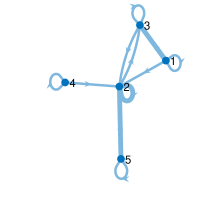
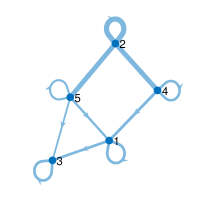
Illustrative example. In Figure 1, we display an illustrative example of the graphical model associated to the following state equations for Nx=5subscript𝑁𝑥5N_{x}=5, for every k1,,K𝑘1𝐾k\in 1,\ldots,K, with 𝐪kNxsubscript𝐪𝑘superscriptsubscript𝑁𝑥{\mathbf{q}}_{k}\in\mathbb{R}^{N_{x}} the latent state noise:

{𝐱k(1)= 0.9𝐱k1(1)+0.7𝐱k1(2)+𝐪k(1),𝐱k(2)=0.3𝐱k1(3)+𝐪k(2),𝐱k(3)= 0.8𝐱k1(5)+𝐪k(3),𝐱k(4)=0.1𝐱k1(2)+𝐪k(4),𝐱k(5)= 0.5𝐱k1(3)+𝐪k(5).casessubscript𝐱𝑘10.9subscript𝐱𝑘110.7subscript𝐱𝑘12subscript𝐪𝑘1otherwisesubscript𝐱𝑘20.3subscript𝐱𝑘13subscript𝐪𝑘2otherwisesubscript𝐱𝑘30.8subscript𝐱𝑘15subscript𝐪𝑘3otherwisesubscript𝐱𝑘40.1subscript𝐱𝑘12subscript𝐪𝑘4otherwisesubscript𝐱𝑘50.5subscript𝐱𝑘13subscript𝐪𝑘5otherwise\begin{cases}{\mathbf{x}}_{k}(1)=\,0.9\,{\mathbf{x}}_{k-1}(1)+0.7{\mathbf{x}}_{k-1}(2)+{\mathbf{q}}_{k}(1),\\ {\mathbf{x}}_{k}(2)=-0.3\,{\mathbf{x}}_{k-1}(3)+{\mathbf{q}}_{k}(2),\\ {\mathbf{x}}_{k}(3)=\,0.8\,{\mathbf{x}}_{k-1}(5)+{\mathbf{q}}_{k}(3),\\ {\mathbf{x}}_{k}(4)=-0.1\,{\mathbf{x}}_{k-1}(2)+{\mathbf{q}}_{k}(4),\\ {\mathbf{x}}_{k}(5)=\,0.5\,{\mathbf{x}}_{k-1}(3)+{\mathbf{q}}_{k}(5).\end{cases} (18)

We display the matrix 𝐀𝐀{\mathbf{A}}, the associated binary matrix supp(𝐀)supp𝐀\rm{supp}({\mathbf{A}}) and the resulting reflexive directed graph under this interpretation.

𝐀=(0.90.7000000.30000000.800.1000000.500)𝐀0.90.7000000.30000000.800.1000000.500{\mathbf{A}}=\left(\begin{array}[]{ccccc}0.9&0.7&0&0&0\\ 0&0&-0.3&0&0\\ 0&0&0&0&0.8\\ 0&-0.1&0&0&0\\ 0&0&0.5&0&0\end{array}\right)
(a) Matrix 𝐀𝐀{\mathbf{A}}.
supp(𝐀)=(1100000100000010100000100)supp𝐀1100000100000010100000100\rm{supp}({\mathbf{A}})=\left(\begin{array}[]{ccccc}1&1&0&0&0\\ 0&0&1&0&0\\ 0&0&0&0&1\\ 0&1&0&0&0\\ 0&0&1&0&0\end{array}\right)

(b) Binary support.
111222333555444A(1,2)𝐴12A(1,2)A(2,3)𝐴23A(2,3)A(4,2)𝐴42A(4,2)A(5,3)𝐴53A(5,3)A(3,5)𝐴35A(3,5)A(1,1)𝐴11A(1,1)
(c) Associated directed graph.
Figure 1: Graphical model associated to (18). Matrix 𝐀𝐀{\mathbf{A}} (a), its binary support (b) and associated reflexive directed graph (c). The edges are defined as non-zero entries of 𝐀superscript𝐀top{\mathbf{A}}^{\top}. Their thickness is proportional to the absolute entries of 𝐀superscript𝐀top{\mathbf{A}}^{\top}.

3.1.2 State noise precision matrix

Matrix 𝐐𝐐{\mathbf{Q}} denotes the noise covariance in the state Eq. (2). Since the noise is assumed to be Gaussian, this matrix, and more precisely, the associated precision matrix 𝐏=𝐐1𝐏superscript𝐐1{\mathbf{P}}={\mathbf{Q}}^{-1}, also has a direct interpretation in terms of graphical modeling, using the notion of Gaussian graphical model (GGM) (Bühlmann and Van De Geer, 2011, Section 13.4)(Uhler, 2017). Since we consider 𝐐𝐐{\mathbf{Q}} constant during the whole time series, let us denote the multivariate state noise r.v. at any time step as 𝐪𝒩(0,𝐐)similar-to𝐪𝒩0𝐐{\mathbf{q}}\sim\mathcal{N}(0,{\mathbf{Q}}). The GGM consists in a graphical modeling of the independence (or not) between the scalar random variables 𝐪(1),,𝐪(Nx)𝐪1𝐪subscript𝑁𝑥{\mathbf{q}}(1),\ldots,{\mathbf{q}}(N_{x}). It is easy to prove that

𝐪(n)𝐪()|{𝐪(j),j1,,Nx\{n,}}𝐏(n,)=𝐏(,n)=0,{\mathbf{q}}(n)\perp\!\!\!\perp{\mathbf{q}}(\ell)|\{{\mathbf{q}}(j),j\in{1,\ldots,N_{x}}\backslash\{n,\ell\}\}\Longleftrightarrow{\mathbf{P}}(n,\ell)={\mathbf{P}}(\ell,n)=0, (19)

i.e., the dimensions n𝑛n and \ell of 𝐪𝐪{\mathbf{q}} are independent given all other dimensions if and only if the entry 𝐏(n,)𝐏𝑛{\mathbf{P}}(n,\ell) is zero (and obviously also 𝐏(,n)𝐏𝑛{\mathbf{P}}(\ell,n) since the precision matrix is symmetric). Note that it is possible to condition in the l.h.s. of (19) only to the dimensions 𝐪(j)𝐪𝑗{\mathbf{q}}(j) for which 𝐏(n,j)0𝐏𝑛𝑗0{\mathbf{P}}(n,j)\neq 0 and the equivalence would still hold. The GGM relies on an undirected graph associated to a symmetric weight matrix equals to the inverse of the covariance matrix 𝐏=𝚺1𝐏superscript𝚺1{\mathbf{P}}={\bm{\Sigma}}^{-1}. In particular, namely (n,)𝔼𝑛𝔼(n,\ell)\notin\mathbb{E} if and only if P(n,)=P(,n)=0𝑃𝑛𝑃𝑛0P(n,\ell)=P(\ell,n)=0.

This GGM construction is at the core of the famous GLASSO (Graphical Lasso) formulation (Friedman et al., 2008)(Maathuis et al., 2019, Section 9.7), whose goal is to build the maximum a posteriori estimator of 𝐏𝐏{\mathbf{P}} given realizations of the random vector 𝐪𝐪{\mathbf{q}} under a sparsity assumption on matrix 𝐏𝐏{\mathbf{P}}. The sparsity is here interpreted as a way to eliminate spurious edges in the graph associated to 𝐏𝐏{\mathbf{P}}.

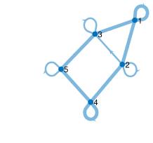
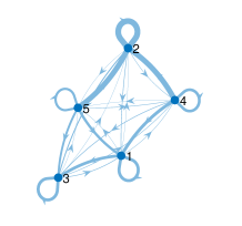
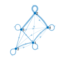
Illustrative example. In Figure 2, we display an illustrative example on the GGM associated to a given precision matrix 𝐏𝐏{\mathbf{P}} for Nx=5subscript𝑁𝑥5N_{x}=5. We show the associated binary support matrix supp(𝐏)supp𝐏\rm{supp}({\mathbf{P}}) and the resulting undirected graph under this interpretation. Although self-loops (i.e., non-zero diagonal elements) occur, we removed them from the graphical representation for ease of readability.

𝐏=(200.10000.90.30.20.50.10.30.80000.202000.5001.5)𝐏200.10000.90.30.20.50.10.30.80000.202000.5001.5{\mathbf{P}}=\left(\begin{array}[]{ccccc}2&0&-0.1&0&0\\ 0&0.9&0.3&-0.2&0.5\\ -0.1&0.3&0.8&0&0\\ 0&-0.2&0&2&0\\ 0&0.5&0&0&1.5\end{array}\right)

(a) Matrix 𝐏𝐏{\mathbf{P}}.
supp(𝐏)=(1010001111111000101001001)supp𝐏1010001111111000101001001\rm{supp}({\mathbf{P}})=\left(\begin{array}[]{ccccc}1&0&1&0&0\\ 0&1&1&1&1\\ 1&1&1&0&0\\ 0&1&0&1&0\\ 0&1&0&0&1\end{array}\right)
(b) Support matrix.
111222333555444A(1,2)𝐴12A(1,2)A(2,3)𝐴23A(2,3)A(4,2)𝐴42A(4,2)A(5,3)𝐴53A(5,3)A(3,5)𝐴35A(3,5)A(1,1)𝐴11A(1,1)111222333555444P(2,5)𝑃25P(2,5)P(2,3)𝑃23P(2,3)P(1,3)𝑃13P(1,3)P(2,4)𝑃24P(2,4)
(c) Associated undirected graph.
Figure 2: Matrix 𝐏𝐏{\mathbf{P}} (a), its binary support (b), and the associated undirected graph (c) with edge thickness proportional to the absolute entries of 𝐏𝐏{\mathbf{P}}.

3.1.3 Proposed unifying view

We now summarize the graphical perspective on both 𝐀𝐀{\mathbf{A}} and 𝐐𝐐{\mathbf{Q}} and describe an unifying approach, where sparsity plays a key role. Matrix 𝐀𝐀{\mathbf{A}} is interpreted as the weight matrix of a directed graph with Nxsubscript𝑁𝑥N_{x} vertices. Sparsity (i.e., absence of edge in the graph) in 𝐀𝐀{\mathbf{A}} is interpreted as pair-wise partial/conditional independence, given a subset of the remaining time series, for a one-step ahead prediction of the hidden state. Matrix 𝐏=𝐐1𝐏superscript𝐐1{\mathbf{P}}={\mathbf{Q}}^{-1} is interpreted as the weight matrix of an undirected graph, related to a GGM describing the noise in the latent space. Sparsity in 𝐏𝐏{\mathbf{P}} is interpreted as pair-wise partial/conditional independence of two dimensions of the additive state noise, given a subset of the remaining dimensions. Both graphs are reflexive, with Nxsubscript𝑁𝑥N_{x} nodes and a maximum of Nx2superscriptsubscript𝑁𝑥2N_{x}^{2} edges for 𝐀𝐀{\mathbf{A}} (Nx(Nx1)subscript𝑁𝑥subscript𝑁𝑥1N_{x}(N_{x}-1) for 𝐏𝐏{\mathbf{P}}) associated to Nx2superscriptsubscript𝑁𝑥2N_{x}^{2} weights (i.e., the Nx2superscriptsubscript𝑁𝑥2N_{x}^{2} entries of 𝐀𝐀{\mathbf{A}} or 𝐏𝐏{\mathbf{P}}).

Our perspective in the state process of the LG-SSM in (2) is that 𝐀𝐀{\mathbf{A}} encodes the way the information flows in consecutive time-steps between the nodes (state dimensions) of the network (vector state). Thus, its properties shape how the energy/information is transferred and dissipated (under the noise). In contrast, 𝐏=𝐐1𝐏superscript𝐐1{\mathbf{P}}={\mathbf{Q}}^{-1} encodes how information that is not in the system at time k1𝑘1k-1 enters in the system at time k𝑘k. In that respect, the interpreted graph with weight matrix 𝐏𝐏{\mathbf{P}} encodes the dependency of the new information across the nodes of the network.

We adopt the above perspective to estimate both 𝐀𝐀{\mathbf{A}} and 𝐐𝐐{\mathbf{Q}} by promoting properties in both graphs. Specifically, we introduce sparsity priors on the matrices, as the sparsity property is key to reach interpretability and compactness of the whole model. In particular, it allows to understand the inner structure of the latent space. Moreover, it can be helpful to speed up computations as the sparsity level is increased, e.g., when running the Kalman filter and RTS smoother. Our proposed method DGLASSO (Dynamic Graphical Lasso) hence aims at providing the maximum a posteriori (MAP) estimator of 𝐀𝐀{\mathbf{A}} and 𝐏𝐏{\mathbf{P}} (i.e., the weight matrices related to the graphical modeling of the latent state correlation and causality) under Lasso sparsity regularization on both matrices, given the observed sequence 𝐲1:Ksubscript𝐲:1𝐾{\mathbf{y}}_{1:K}. A visual representation of DGLASSO graphical model is given in Figure 3. The figure summarizes the relationships among the state entries of an LG-SSM using matrices (𝐀,𝐏)𝐀𝐏({\mathbf{A}},{\mathbf{P}}) from Figures 1 and 2.

Related works:

Our approach DGLASSO generalizes important existing sparse graphical inference ones. For instance, our model with 𝐀=0𝐀0{\mathbf{A}}=0 (degenerate case) has no memory, and all the energy/information of the system is lost at each time step, thus the state dimensions only incorporate exogenous energy/information through the additive noises. This degenerate case is the same model than GLASSO (Friedman et al., 2008) in the case when 𝐑k0subscript𝐑𝑘0{\mathbf{R}}_{k}\equiv 0, and same than the robust GLASSO model (Benfenati et al., 2020, Sec.5.2) when 𝐑kσR2𝐈𝐝subscript𝐑𝑘superscriptsubscript𝜎𝑅2𝐈𝐝{\mathbf{R}}_{k}\equiv\sigma_{R}^{2}\bf{Id}. In contrast, if the state noise covariance matrix 𝐐𝐐{\mathbf{Q}} is known, DGLASSO coincides with our recent GraphEM framework (Elvira and Chouzenoux, 2022). Probably the closer related work is (Ioannidis et al., 2019), which also introduces a joint graph modeling within an LG-SSM, capturing order-one causal relationships and instantaneous influence (i.e., order zero), through two sparse graphs. Their proposed inference method is an alternating optimization technique, that infers the two graphs under Lasso prior, jointly with the estimation of hidden state. In contrast with DGLASSO, in (Ioannidis et al., 2019), (i) the state model follows a structural vector autoregressive model (SVAR) where instantaneous causality and noise are distinguished, while DGLASSO assumes an order-one VAR in the hidden state; and (ii) the cost function does not result from a Bayesian modeling, and as such it is not related to a maximum a posteriori loss for the graph variables, (iii) the state estimation is point wise defined as the solution of an handcrafted optimization problem, while DGLASSO preserves a full Bayesian interpretation and hence allows the complete characterization of the filtering/smoothing state distributions. In particular, (Ioannidis et al., 2019) model does not recover GLASSO as a particular case.

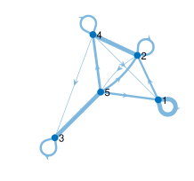
111222333555444A(1,2)𝐴12A(1,2)A(2,3)𝐴23A(2,3)A(4,2)𝐴42A(4,2)A(5,3)𝐴53A(5,3)A(3,5)𝐴35A(3,5)A(1,1)𝐴11A(1,1)111222333555444P(2,5)𝑃25P(2,5)P(2,3)𝑃23P(2,3)P(1,3)𝑃13P(1,3)P(2,4)𝑃24P(2,4) 𝐱k1(1)subscript𝐱𝑘11{\mathbf{x}}_{k-1}(1) 𝐱k1(2)subscript𝐱𝑘12{\mathbf{x}}_{k-1}(2) 𝐱k=1(3)subscript𝐱𝑘13{\mathbf{x}}_{k=1}(3) 𝐱k1(4)subscript𝐱𝑘14{\mathbf{x}}_{k-1}(4) 𝐱k1(5)subscript𝐱𝑘15{\mathbf{x}}_{k-1}(5) 𝐱k(1)subscript𝐱𝑘1{\mathbf{x}}_{k}(1) 𝐱k(2)subscript𝐱𝑘2{\mathbf{x}}_{k}(2) 𝐱k(3)subscript𝐱𝑘3{\mathbf{x}}_{k}(3) 𝐱k(4)subscript𝐱𝑘4{\mathbf{x}}_{k}(4) 𝐱k(5)subscript𝐱𝑘5{\mathbf{x}}_{k}(5) 𝐱k+1(1)subscript𝐱𝑘11{\mathbf{x}}_{k+1}(1) 𝐱k+1(2)subscript𝐱𝑘12{\mathbf{x}}_{k+1}(2) 𝐱k+1(3)subscript𝐱𝑘13{\mathbf{x}}_{k+1}(3) 𝐱k+1(4)subscript𝐱𝑘14{\mathbf{x}}_{k+1}(4) 𝐱k+1(5)subscript𝐱𝑘15{\mathbf{x}}_{k+1}(5)
Figure 3: Summary representation of the DGLASSO graphical model, for the example graphs presented in Figs. 1 and 2. Blue (oriented) edges represent Granger causality between state entries among consecutive time steps, encoded in matrix 𝐀𝐀{\mathbf{A}} (Fig. 1). Magenta edges represent static (i.e., instantaneous) relationships between the state entries, at every time step, due to correlated state noise described by matrix 𝐏𝐏{\mathbf{P}} (Fig. 2).

3.2 Optimization problem

The considered MAP inference problem reads as an optimization problem that we formulate hereafter. More specifically, let us denote the posterior of the unknown parameter, p(𝐀,𝐏|𝐲1:K)𝑝𝐀conditional𝐏subscript𝐲:1𝐾p({\mathbf{A}},{\mathbf{P}}|{\mathbf{y}}_{1:K}), where the hidden states have been marginalized. It is direct to show, using Bayes rule and composition with the (strictly increasing) logarithmic function, that the maximum of p(𝐀,𝐏|𝐲1:K)p(𝐀,𝐏)p(𝐲1:K|𝐀,𝐏)proportional-to𝑝𝐀conditional𝐏subscript𝐲:1𝐾𝑝𝐀𝐏𝑝conditionalsubscript𝐲:1𝐾𝐀𝐏p({\mathbf{A}},{\mathbf{P}}|{\mathbf{y}}_{1:K})\propto p({\mathbf{A}},{\mathbf{P}})p({\mathbf{y}}_{1:K}|{\mathbf{A}},{\mathbf{P}}), with p(𝐀,𝐏)𝑝𝐀𝐏p({\mathbf{A}},{\mathbf{P}}) some prior on the parameters 𝐀𝐀{\mathbf{A}} and 𝐏𝐏{\mathbf{P}}, coincides with the minimum of the following loss function:

(𝐀Nx×Nx)(𝐏𝒮Nx)(𝐀,𝐏)for-all𝐀superscriptsubscript𝑁𝑥subscript𝑁𝑥for-all𝐏subscript𝒮subscript𝑁𝑥𝐀𝐏\displaystyle(\forall{\mathbf{A}}\in\mathbb{R}^{N_{x}\times N_{x}})(\forall{\mathbf{P}}\in\mathcal{S}_{N_{x}})\quad\mathcal{L}({\mathbf{A}},{\mathbf{P}}) 1:K(𝐀,𝐏)+0(𝐀,𝐏).absentsubscript:1𝐾𝐀𝐏subscript0𝐀𝐏\displaystyle\triangleq\mathcal{L}_{1:K}({\mathbf{A}},{\mathbf{P}})+\mathcal{L}_{0}({\mathbf{A}},{\mathbf{P}}). (20)

with 1:K(𝐀,𝐏)logp(𝐲1:K|𝐀,𝐏)subscript:1𝐾𝐀𝐏𝑝conditionalsubscript𝐲:1𝐾𝐀𝐏\mathcal{L}_{1:K}({\mathbf{A}},{\mathbf{P}})\triangleq-\log p({\mathbf{y}}_{1:K}|{\mathbf{A}},{\mathbf{P}}) and 0(𝐀,𝐏)=logp(𝐀,𝐏)subscript0𝐀𝐏𝑝𝐀𝐏\mathcal{L}_{0}({\mathbf{A}},{\mathbf{P}})=-\log p({\mathbf{A}},{\mathbf{P}}). According to (Sarkka, 2013, Chap. 12),

(𝐀Nx×Nx)(𝐏𝒮Nx)1:K(𝐀,𝐏)=k=1K12logdet(2π𝐒k)+12𝐳k𝐒k1𝐳k,for-all𝐀superscriptsubscript𝑁𝑥subscript𝑁𝑥for-all𝐏subscript𝒮subscript𝑁𝑥subscript:1𝐾𝐀𝐏superscriptsubscript𝑘1𝐾122𝜋subscript𝐒𝑘12superscriptsubscript𝐳𝑘topsuperscriptsubscript𝐒𝑘1subscript𝐳𝑘(\forall{\mathbf{A}}\in\mathbb{R}^{N_{x}\times N_{x}})(\forall{\mathbf{P}}\in\mathcal{S}_{N_{x}})\quad\mathcal{L}_{1:K}({\mathbf{A}},{\mathbf{P}})=\sum_{k=1}^{K}\tfrac{1}{2}\log\det(2\pi{\mathbf{S}}_{k})+\frac{1}{2}{\mathbf{z}}_{k}^{\top}{\mathbf{S}}_{k}^{-1}{\mathbf{z}}_{k}, (21)

where 𝐳k=𝐲k𝐇k𝐀𝝁k1subscript𝐳𝑘subscript𝐲𝑘subscript𝐇𝑘𝐀subscript𝝁𝑘1{\mathbf{z}}_{k}={\mathbf{y}}_{k}-{\mathbf{H}}_{k}{\mathbf{A}}\bm{\mu}_{k-1} and 𝐒ksubscript𝐒𝑘{\mathbf{S}}_{k} is the covariance matrix of the predictive distribution p(𝐲k|𝐲1:k1,𝐀,𝐏)=𝒩(𝐲k;𝐇𝐀𝝁k1,𝐒k)𝑝conditionalsubscript𝐲𝑘subscript𝐲:1𝑘1𝐀𝐏𝒩subscript𝐲𝑘𝐇𝐀subscript𝝁𝑘1subscript𝐒𝑘p({\mathbf{y}}_{k}|{\mathbf{y}}_{1:k-1},{\mathbf{A}},{\mathbf{P}})=\mathcal{N}\left({\mathbf{y}}_{k};{\mathbf{H}}{\mathbf{A}}\bm{\mu}_{k-1},{\mathbf{S}}_{k}\right), both being obtained by the KF in Alg. 1 run for given (𝐀,𝐏)𝐀𝐏({\mathbf{A}},{\mathbf{P}}) (see (Sarkka, 2013, Section 4.3)).

As already mentioned, the introduction of priors that induce sparsity is advantageous due to several reasons. First, it generally reduces over-fitting, particularly when K𝐾K is low compared to the number of parameters to be estimated. Also, it enhances the interpretability. The zero elements in 𝐀𝐀{\mathbf{A}} and 𝐏𝐏{\mathbf{P}} have a clear interpretation of conditional independence between the time series. Ideally, we would use the 0subscript0\ell_{0} norm of 𝐀𝐀{\mathbf{A}} and 𝐏𝐏{\mathbf{P}}, i.e., penalizing the number of non-zero entries of the matrix. However, this norm is known to have undesirable properties such as being non-convex, non continuous, and associated to a improper law p(𝐀)𝑝𝐀p({\mathbf{A}}). We thus propose instead the regularization term

(𝐀Nx×Nx)(𝐏𝒮Nx)0(𝐀,𝐏)=λA𝐀1+λP𝐏1.for-all𝐀superscriptsubscript𝑁𝑥subscript𝑁𝑥for-all𝐏subscript𝒮subscript𝑁𝑥subscript0𝐀𝐏subscript𝜆𝐴subscriptnorm𝐀1subscript𝜆𝑃subscriptnorm𝐏1(\forall{\mathbf{A}}\in\mathbb{R}^{N_{x}\times N_{x}})(\forall{\mathbf{P}}\in\mathcal{S}_{N_{x}})\quad\mathcal{L}_{0}({\mathbf{A}},{\mathbf{P}})=\lambda_{A}\|{\mathbf{A}}\|_{1}+\lambda_{P}\|{\mathbf{P}}\|_{1}. (22)

The 1subscript1\ell_{1} norm in (22), defined as the sum of absolute values of the matrix entries, is a proper convex function, that leads to the so-called Lasso regularization (Bach et al., 2012). Note that this penalty, used in numerous works of signal processing and machine learning (Tibshirani, 1996; Chaux et al., 2007), including graph signal processing (Friedman et al., 2008; Benfenati et al., 2020), is associated with a joint Laplace prior distribution on 𝐀𝐀{\mathbf{A}} and 𝐏𝐏{\mathbf{P}}. Such joint distribution factorizes (i.e., the prior assumes independence on both parameters), the means are zero, and the scale parameters are proportional to, respectively, λAsubscript𝜆𝐴\lambda_{A} and λPsubscript𝜆𝑃\lambda_{P}. The larger the regularization parameter λAsubscript𝜆𝐴\lambda_{A} (or λP)\lambda_{P}), the higher sparsity of 𝐀𝐀{\mathbf{A}} (or 𝐏){\mathbf{P}}), with the degenerate case of a null 𝐀𝐀{\mathbf{A}} (and 𝐏𝐏{\mathbf{P}}) when the regularization parameter grows.

3.3 General minimization procedure

The expressions (21)-(22) provide an effective way to evaluate (20). However, due to the recursive form in (21), it is challenging to derive direct quantities (e.g., gradient) for 1:Ksubscript:1𝐾\mathcal{L}_{1:K}. Moreover, despite its simple expression, the regularization term (22) is non differentiable. For both reasons, the minimization of (20) is a challenging question.

We propose a block alternating majorization-minimization (MM) technique to jointly infer the probabilistic filtering/smoothing distributions of the SSM, along with MAP estimates of (𝐀,𝐏)𝐀𝐏({\mathbf{A}},{\mathbf{P}}). Our method presents the advantage of sound convergence guarantees and the ability to incorporate sparsity priors on both 𝐀𝐀{\mathbf{A}} and 𝐏𝐏{\mathbf{P}}. The general idea of MM is to replace a complicated optimization problem by a sequence of more tractable ones (Sun et al., 2016; Hunter and Lange, 2004). Surrogate approximations of the cost function are built iteratively, following a majorization principle. For any estimates 𝐀~Nx×Nx~𝐀superscriptsubscript𝑁𝑥subscript𝑁𝑥\widetilde{{\mathbf{A}}}\in\mathbb{R}^{N_{x}\times N_{x}} and 𝐏~𝒮Nx++~𝐏superscriptsubscript𝒮subscript𝑁𝑥absent\widetilde{{\mathbf{P}}}\in\mathcal{S}_{N_{x}}^{++} (i.e., in the interior domain of definition of \mathcal{L}) of (𝐀,𝐏)𝐀𝐏({\mathbf{A}},{\mathbf{P}}), a majorizing approximation is constructed for the likelihood term. It is required to satisfy both

(𝐀Nx×Nx)(𝐏𝒮Nx)𝒬(𝐀,𝐏;𝐀~,𝐏~)1:K(𝐀,𝐏),for-all𝐀superscriptsubscript𝑁𝑥subscript𝑁𝑥for-all𝐏subscript𝒮subscript𝑁𝑥𝒬𝐀𝐏~𝐀~𝐏subscript:1𝐾𝐀𝐏(\forall{\mathbf{A}}\in\mathbb{R}^{N_{x}\times N_{x}})(\forall{\mathbf{P}}\in\mathcal{S}_{N_{x}})\quad\mathcal{Q}({\mathbf{A}},{\mathbf{P}};\widetilde{{\mathbf{A}}},\widetilde{{\mathbf{P}}})\geq\mathcal{L}_{1:K}({\mathbf{A}},{\mathbf{P}}), (23)

and also the so-called tangency condition

𝒬(𝐀~,𝐏~;𝐀~,𝐏~)=1:K(𝐀~,𝐏~).𝒬~𝐀~𝐏~𝐀~𝐏subscript:1𝐾~𝐀~𝐏\mathcal{Q}(\widetilde{{\mathbf{A}}},\widetilde{{\mathbf{P}}};\widetilde{{\mathbf{A}}},\widetilde{{\mathbf{P}}})=\mathcal{L}_{1:K}(\widetilde{{\mathbf{A}}},\widetilde{{\mathbf{P}}}). (24)

The MM algorithm then alternates between Majorization step to build function 𝒬+0𝒬subscript0\mathcal{Q}+\mathcal{L}_{0} satisfying conditions (23) and (24), and Minimization step to minimize this majorizing approximation. In our proposed approach, we adopt a block alternating implementation of the MM method, where only one variable (i.e., 𝐀𝐀{\mathbf{A}} or 𝐏𝐏{\mathbf{P}}) is updated at each iteration, following a cyclic rule (Jacobson and Fessler, 2007; Hong et al., 2016). This alternating strategy considerably simplifies the majorizing function construction as well as its minimization. We furthermore add so-called proximal terms in both updates. Let us recall that, for a function ϕ:(,+]Γ0():italic-ϕmaps-tosubscriptΓ0\phi:\mathcal{H}\mapsto(-\infty,+\infty]\in\Gamma_{0}(\mathcal{H}), with \mathcal{H} a Hilbert space with endowed norm \|\cdot\|, the proximity operator222See also http://proximity-operator.net/ of function f𝑓f at 𝐕~~𝐕\widetilde{{\mathbf{V}}}\in\mathcal{H} is defined as (Combettes and Pesquet, 2011)

proxϕ(𝐕~)=argmin𝐕(ϕ(𝐕)+12𝐕𝐕~2).subscriptproxitalic-ϕ~𝐕𝐕argminitalic-ϕ𝐕12superscriptnorm𝐕~𝐕2\operatorname{prox}_{\phi}(\widetilde{{\mathbf{V}}})=\underset{\begin{subarray}{c}{{\mathbf{V}}\in\mathcal{H}}\end{subarray}}{\operatorname{argmin}}\;\;\left(\phi({\mathbf{V}})+\frac{1}{2}\|{\mathbf{V}}-\widetilde{{\mathbf{V}}}\|^{2}\right). (25)

In our context, the considered Hilbert space is either Nx×Nxsuperscriptsubscript𝑁𝑥subscript𝑁𝑥\mathbb{R}^{N_{x}\times N_{x}} for the update of the transition matrix or 𝒮Nxsubscript𝒮subscript𝑁𝑥\mathcal{S}_{N_{x}} for the update of the precision matrix, and the endowed norm is in both cases the Frobenius norm F\|\cdot\|_{F}. Introducing proximity terms thus amounts to adding to each majorizing function a quadratic distance to the previous iterate, weighted by a positive factor. This modification preserves the MM interpretation of the method, while ensuring improved stability and convergence guarantees. As we show below, the iterates belong to the interior of domain of the loss function by construction. Namely for every i𝑖i\in\mathbb{N}, (𝐀(i),𝐏(i))Nx×Nx×𝒮Nx++superscript𝐀𝑖superscript𝐏𝑖superscriptsubscript𝑁𝑥subscript𝑁𝑥superscriptsubscript𝒮subscript𝑁𝑥absent({\mathbf{A}}^{(i)},{\mathbf{P}}^{(i)})\in\mathbb{R}^{N_{x}\times N_{x}}\times\mathcal{S}_{N_{x}}^{++}, so the precision matrix remains invertible along the iterations and the algorithm is well defined. The resulting DGLASSO approach is summarized in Algorithm 3. DGLASSO aims at providing ultimately the MAP estimates for the matrix parameters (𝐀,𝐏)𝐀𝐏({\mathbf{A}},{\mathbf{P}}) of the considered LG-SSM, through the minimization of (20). The covariance state noise MAP estimate is straightforwardly obtained by inversion of the precision state noise matrix provided as an output of DGLASSO. The state filtering/smoothing pdf associated to each estimates are obtained by running KF/RTS loops when setting (𝐀,𝐏)𝐀𝐏({\mathbf{A}},{\mathbf{P}}) equal to DGLASSO outputs. Next sections are dedicated to the (i) construction of the majorizing function, (ii) discussion about the resolution of each inner step, and (iii) convergence analysis.

Algorithm 3
DGLASSO algorithm Inputs. Prior parameters 𝝁0subscript𝝁0\bm{\mu}_{0} and 𝚺0subscript𝚺0{\bm{\Sigma}}_{0}; model parameters {𝐇k}k=1Ksuperscriptsubscriptsubscript𝐇𝑘𝑘1𝐾\{{\mathbf{H}}_{k}\}_{k=1}^{K} and {𝐑k}k=1Ksuperscriptsubscriptsubscript𝐑𝑘𝑘1𝐾\{{\mathbf{R}}_{k}\}_{k=1}^{K}; set of observations {𝐲k}k=1Ksuperscriptsubscriptsubscript𝐲𝑘𝑘1𝐾\{{\mathbf{y}}_{k}\}_{k=1}^{K}; hyper-parameters (λA,λP)>0subscript𝜆𝐴subscript𝜆𝑃0(\lambda_{A},\lambda_{P})>0; stepsizes (θA,θP)>0subscript𝜃𝐴subscript𝜃𝑃0(\theta_{A},\theta_{P})>0; precisions (ε,ξ)>0𝜀𝜉0(\varepsilon,\xi)>0. Initialization. Set (𝐀(0),𝐏(0))Nx×Nx×𝒮Nx++superscript𝐀0superscript𝐏0superscriptsubscript𝑁𝑥subscript𝑁𝑥superscriptsubscript𝒮subscript𝑁𝑥absent({\mathbf{A}}^{(0)},{\mathbf{P}}^{(0)})\in\mathbb{R}^{N_{x}\times N_{x}}\times\mathcal{S}_{N_{x}}^{++}. Recursive step. For i=0,1,𝑖01i=0,1,\ldots: (a) //Update transition matrix (i) Build surrogate function satisfying (23) and (24) at 𝐀~=𝐀(i)~𝐀superscript𝐀𝑖\widetilde{{\mathbf{A}}}={\mathbf{A}}^{(i)} and 𝐏~=𝐏(i)~𝐏superscript𝐏𝑖\widetilde{{\mathbf{P}}}={\mathbf{P}}^{(i)}. (ii) Run Algorithm 4 with precision ξ𝜉\xi to solve 𝐀(i+1)=prox𝐀θA𝒬(𝐀,𝐏(i);𝐀(i),𝐏(i))+θAλA𝐀1(𝐀(i)),=argmin𝐀Nx×Nx𝒬(𝐀,𝐏(i);𝐀(i),𝐏(i))+λA𝐀1+12θA𝐀𝐀(i)F2.superscript𝐀𝑖1absentsubscriptprox𝐀subscript𝜃𝐴𝒬𝐀superscript𝐏𝑖superscript𝐀𝑖superscript𝐏𝑖subscript𝜃𝐴subscript𝜆𝐴subscriptnorm𝐀1superscript𝐀𝑖missing-subexpressionabsent𝐀superscriptsubscript𝑁𝑥subscript𝑁𝑥argmin𝒬𝐀superscript𝐏𝑖superscript𝐀𝑖superscript𝐏𝑖subscript𝜆𝐴subscriptnorm𝐀112subscript𝜃𝐴subscriptsuperscriptnorm𝐀superscript𝐀𝑖2𝐹\begin{array}[]{ll}{\mathbf{A}}^{(i+1)}&=\operatorname{prox}_{{\mathbf{A}}\to\theta_{A}\mathcal{Q}({\mathbf{A}},{\mathbf{P}}^{(i)};{\mathbf{A}}^{(i)},{\mathbf{P}}^{(i)})+\theta_{A}\lambda_{A}\|{\mathbf{A}}\|_{1}}\left({\mathbf{A}}^{(i)}\right),\\ &=\underset{\begin{subarray}{c}{{\mathbf{A}}\in\mathbb{R}^{N_{x}\times N_{x}}}\end{subarray}}{\operatorname{argmin}}\;\;\mathcal{Q}({\mathbf{A}},{\mathbf{P}}^{(i)};{\mathbf{A}}^{(i)},{\mathbf{P}}^{(i)})+\lambda_{A}\|{\mathbf{A}}\|_{1}+\frac{1}{2\theta_{A}}\|{\mathbf{A}}-{\mathbf{A}}^{(i)}\|^{2}_{F}.\end{array} (26) (b) //Update noise precision matrix (i) Build surrogate function satisfying (23) and (24) at 𝐀~=𝐀(i+1)~𝐀superscript𝐀𝑖1\widetilde{{\mathbf{A}}}={\mathbf{A}}^{(i+1)} and 𝐏~=𝐏(i)~𝐏superscript𝐏𝑖\widetilde{{\mathbf{P}}}={\mathbf{P}}^{(i)}. (ii) Run Algorithm 5 with precision ξ𝜉\xi to solve 𝐏(i+1)=prox𝐏θP𝒬(𝐀(i+1),𝐏;𝐀(i+1),𝐏(i))+θPλP𝐏1(𝐏(i)),=argmin𝐏𝒮Nx𝒬(𝐀(i+1),𝐏;𝐀(i+1),𝐏(i))+λP𝐏1+12θP𝐏𝐏(i)F2.superscript𝐏𝑖1absentsubscriptprox𝐏subscript𝜃𝑃𝒬superscript𝐀𝑖1𝐏superscript𝐀𝑖1superscript𝐏𝑖subscript𝜃𝑃subscript𝜆𝑃subscriptnorm𝐏1superscript𝐏𝑖missing-subexpressionabsent𝐏subscript𝒮subscript𝑁𝑥argmin𝒬superscript𝐀𝑖1𝐏superscript𝐀𝑖1superscript𝐏𝑖subscript𝜆𝑃subscriptnorm𝐏112subscript𝜃𝑃subscriptsuperscriptnorm𝐏superscript𝐏𝑖2𝐹\begin{array}[]{ll}{\mathbf{P}}^{(i+1)}&=\operatorname{prox}_{{\mathbf{P}}\to\theta_{P}\mathcal{Q}({\mathbf{A}}^{(i+1)},{\mathbf{P}};{\mathbf{A}}^{(i+1)},{\mathbf{P}}^{(i)})+\theta_{P}\lambda_{P}\|{\mathbf{P}}\|_{1}}\left({\mathbf{P}}^{(i)}\right),\\ &=\underset{\begin{subarray}{c}{{\mathbf{P}}\in\mathcal{S}_{N_{x}}}\end{subarray}}{\operatorname{argmin}}\;\;\mathcal{Q}({\mathbf{A}}^{(i+1)},{\mathbf{P}};{\mathbf{A}}^{(i+1)},{\mathbf{P}}^{(i)})+\lambda_{P}\|{\mathbf{P}}\|_{1}+\frac{1}{2\theta_{P}}\|{\mathbf{P}}-{\mathbf{P}}^{(i)}\|^{2}_{F}.\end{array} (27) If 𝐀(i+1)𝐀(i)Fε𝐀(i)Fsubscriptnormsuperscript𝐀𝑖1superscript𝐀𝑖𝐹𝜀subscriptnormsuperscript𝐀𝑖𝐹\|{\mathbf{A}}^{(i+1)}-{\mathbf{A}}^{(i)}\|_{F}\leq\varepsilon\|{\mathbf{A}}^{(i)}\|_{F} and 𝐏(i+1)𝐏(i)Fε𝐏(i)Fsubscriptnormsuperscript𝐏𝑖1superscript𝐏𝑖𝐹𝜀subscriptnormsuperscript𝐏𝑖𝐹\|{\mathbf{P}}^{(i+1)}-{\mathbf{P}}^{(i)}\|_{F}\leq\varepsilon\|{\mathbf{P}}^{(i)}\|_{F}, stop the recursion by returning (𝐀(i+1),𝐏(i+1))superscript𝐀𝑖1superscript𝐏𝑖1({\mathbf{A}}^{(i+1)},{\mathbf{P}}^{(i+1)}). Output. MAP estimates of the transition and state noise precision matrices.

3.4 Building the majorizing function

In this section, we derive a theorem regarding the expression of the loss function 1:Ksubscript:1𝐾\mathcal{L}_{1:K} and a valid majorant function for it.

Theorem 1

The loss function can be expressed as

(𝐀Nx×Nx)(𝐏𝒮Nx)1:K(𝐀,𝐏)=12k=1K((𝐱k𝐀𝐱k1)𝐏(𝐱k𝐀𝐱k1))K2logdet(2π𝐏)+logp(𝐱0:K|𝐲1:K,𝐀,𝐏)+logp(𝐱0)k=1Kp(𝐲k|𝐱k).for-all𝐀superscriptsubscript𝑁𝑥subscript𝑁𝑥for-all𝐏subscript𝒮subscript𝑁𝑥subscript:1𝐾𝐀𝐏12superscriptsubscript𝑘1𝐾superscriptsubscript𝐱𝑘subscript𝐀𝐱𝑘1top𝐏subscript𝐱𝑘subscript𝐀𝐱𝑘1𝐾22𝜋𝐏𝑝conditionalsubscript𝐱:0𝐾subscript𝐲:1𝐾𝐀𝐏𝑝subscript𝐱0superscriptsubscript𝑘1𝐾𝑝conditionalsubscript𝐲𝑘subscript𝐱𝑘(\forall{\mathbf{A}}\in\mathbb{R}^{N_{x}\times N_{x}})(\forall{\mathbf{P}}\in\mathcal{S}_{N_{x}})\quad\mathcal{L}_{1:K}({\mathbf{A}},{\mathbf{P}})=\frac{{1}}{2}\sum_{k=1}^{K}\left(\left({\mathbf{x}}_{k}-{\mathbf{A}}{\mathbf{x}}_{k-1}\right)^{\top}{\mathbf{P}}\left({\mathbf{x}}_{k}-{\mathbf{A}}{\mathbf{x}}_{k-1}\right)\right)\\ -\frac{K}{2}\log\det({2\pi}{{\mathbf{P}}})+\log p({\mathbf{x}}_{0:K}|{\mathbf{y}}_{1:K},{\mathbf{A}},{\mathbf{P}})+\log p({\mathbf{x}}_{0})-\sum_{k=1}^{K}p({\mathbf{y}}_{k}|{\mathbf{x}}_{k}). (28)

Moreover, consider the outputs of Algs. 1 and 2 for a given 𝐀~Nx×Nx~𝐀superscriptsubscript𝑁𝑥subscript𝑁𝑥\widetilde{{\mathbf{A}}}\in\mathbb{R}^{N_{x}\times N_{x}} and 𝐏~𝒮Nx++~𝐏subscript𝒮superscriptsubscript𝑁𝑥absent\widetilde{{\mathbf{P}}}\in\mathcal{S}_{N_{x}^{++}}. Denote

{𝚿=1Kk=1K(𝚺ks+𝝁ks(𝝁ks)),𝚫=1Kk=1K(𝚺ks𝐆k1+𝝁ks(𝝁k1s)),𝚽=1Kk=1K(𝚺k1s+𝝁k1s(𝝁k1s)),cases𝚿absent1𝐾superscriptsubscript𝑘1𝐾subscriptsuperscript𝚺s𝑘subscriptsuperscript𝝁s𝑘superscriptsubscriptsuperscript𝝁s𝑘top𝚫absent1𝐾superscriptsubscript𝑘1𝐾subscriptsuperscript𝚺s𝑘superscriptsubscript𝐆𝑘1topsubscriptsuperscript𝝁s𝑘superscriptsubscriptsuperscript𝝁s𝑘1top𝚽absent1𝐾superscriptsubscript𝑘1𝐾subscriptsuperscript𝚺s𝑘1subscriptsuperscript𝝁s𝑘1superscriptsubscriptsuperscript𝝁s𝑘1top\begin{cases}{\bm{\Psi}}&=\frac{1}{K}\sum_{k=1}^{K}\left({\bm{\Sigma}}^{\text{s}}_{k}+\bm{\mu}^{\text{s}}_{k}(\bm{\mu}^{\text{s}}_{k})^{\top}\right),\\ {\bm{\Delta}}&=\frac{1}{K}\sum_{k=1}^{K}\left({\bm{\Sigma}}^{\text{s}}_{k}{\mathbf{G}}_{k-1}^{\top}+\bm{\mu}^{\text{s}}_{k}(\bm{\mu}^{\text{s}}_{k-1})^{\top}\right),\\ {\bm{\Phi}}&=\frac{1}{K}\sum_{k=1}^{K}\left({\bm{\Sigma}}^{\text{s}}_{k-1}+\bm{\mu}^{\text{s}}_{k-1}(\bm{\mu}^{\text{s}}_{k-1})^{\top}\right),\end{cases} (29)

where, for every k{1,,K}𝑘1𝐾k\in\{1,\ldots,K\}, 𝐆k=𝚺k𝐀~(𝐀~𝚺k𝐀~+𝐏~1)1subscript𝐆𝑘subscript𝚺𝑘superscript~𝐀topsuperscript~𝐀subscript𝚺𝑘superscript~𝐀topsuperscript~𝐏11{\mathbf{G}}_{k}={\bm{\Sigma}}_{k}\widetilde{{\mathbf{A}}}^{\top}(\widetilde{{\mathbf{A}}}{\bm{\Sigma}}_{k}\widetilde{{\mathbf{A}}}^{\top}+\widetilde{{\mathbf{P}}}^{-1})^{-1} (see Alg. 2). Then, conditions (23) and (24) hold with

(𝐀Nx×Nx)(𝐏𝒮Nx)𝒬(𝐀,𝐏;𝐀~,𝐏~)=K2tr(𝐏(𝚿𝚫𝐀𝐀𝚫+𝐀𝚽𝐀))K2logdet(2π𝐏).for-all𝐀superscriptsubscript𝑁𝑥subscript𝑁𝑥for-all𝐏subscript𝒮subscript𝑁𝑥𝒬𝐀𝐏~𝐀~𝐏𝐾2tr𝐏𝚿𝚫superscript𝐀top𝐀superscript𝚫top𝐀𝚽superscript𝐀top𝐾22𝜋𝐏(\forall{\mathbf{A}}\in\mathbb{R}^{N_{x}\times N_{x}})(\forall{\mathbf{P}}\in\mathcal{S}_{N_{x}})\quad\mathcal{Q}({\mathbf{A}},{\mathbf{P}};\widetilde{{\mathbf{A}}},\widetilde{{\mathbf{P}}})=\frac{K}{2}\operatorname{tr}\left({\mathbf{P}}({\bm{\Psi}}-{\bm{\Delta}}{\mathbf{A}}^{\top}-{\mathbf{A}}{\bm{\Delta}}^{\top}+{\mathbf{A}}{\bm{\Phi}}{\mathbf{A}}^{\top})\right)\\ -\frac{K}{2}\log\det({2\pi}{{\mathbf{P}}}). (30)

As a consequence, for every (θA,θP)>0subscript𝜃𝐴subscript𝜃𝑃0(\theta_{A},\theta_{P})>0,

(𝐀Nx×Nx)(𝐏𝒮Nx)(𝐀,𝐏)𝒬(𝐀,𝐏;𝐀~,𝐏~)+1:K(𝐀~,𝐏~)𝒬(𝐀~,𝐏~;𝐀~,𝐏~)+λA𝐀1+λP𝐏1+12θA𝐀𝐀~F2+12θP𝐏𝐏~F2,for-all𝐀superscriptsubscript𝑁𝑥subscript𝑁𝑥for-all𝐏subscript𝒮subscript𝑁𝑥𝐀𝐏𝒬𝐀𝐏~𝐀~𝐏subscript:1𝐾~𝐀~𝐏𝒬~𝐀~𝐏~𝐀~𝐏subscript𝜆𝐴subscriptdelimited-∥∥𝐀1subscript𝜆𝑃subscriptdelimited-∥∥𝐏112subscript𝜃𝐴subscriptsuperscriptdelimited-∥∥𝐀~𝐀2𝐹12subscript𝜃𝑃subscriptsuperscriptdelimited-∥∥𝐏~𝐏2𝐹(\forall{\mathbf{A}}\in\mathbb{R}^{N_{x}\times N_{x}})(\forall{\mathbf{P}}\in\mathcal{S}_{N_{x}})\quad\mathcal{L}({\mathbf{A}},{\mathbf{P}})\leq\mathcal{Q}({\mathbf{A}},{\mathbf{P}};\widetilde{{\mathbf{A}}},\widetilde{{\mathbf{P}}})+\mathcal{L}_{1:K}(\widetilde{{\mathbf{A}}},\widetilde{{\mathbf{P}}})-\mathcal{Q}(\widetilde{{\mathbf{A}}},\widetilde{{\mathbf{P}}};\widetilde{{\mathbf{A}}},\widetilde{{\mathbf{P}}})\\ +\lambda_{A}\|{\mathbf{A}}\|_{1}+\lambda_{P}\|{\mathbf{P}}\|_{1}+\frac{1}{2\theta_{A}}\|{\mathbf{A}}-\widetilde{{\mathbf{A}}}\|^{2}_{F}+\frac{1}{2\theta_{P}}\|{\mathbf{P}}-\widetilde{{\mathbf{P}}}\|^{2}_{F}, (31)

with equality holding for 𝐀=𝐀~𝐀~𝐀{\mathbf{A}}=\widetilde{{\mathbf{A}}} and 𝐏=𝐏~𝐏~𝐏{\mathbf{P}}=\widetilde{{\mathbf{P}}}.

Proof  See Appendix A.  

Theorem 1 allows to build, for any tangent point (𝐀~,𝐏~)~𝐀~𝐏(\widetilde{{\mathbf{A}}},\widetilde{{\mathbf{P}}}), a majorizing approximation (31) for \mathcal{L}. DGLASSO method leverages this property designing a block alternating MM scheme. At each iteration i𝑖i\in\mathbb{N}, two steps are conducted, namely the update of (a) the transition matrix, (b) the noise precision matrix. Each steps follows an MM structure, that is it first builds a majorizing approximation for \mathcal{L} at the current estimates, using Theorem 1, and then minimizes it with respect to the active variable (𝐀𝐀{\mathbf{A}} in step (a), or 𝐏𝐏{\mathbf{P}} in step (b)). Processing the variables in two distinct steps allows to build upon the desirable convex structure of (31) with respect to one of the variable, the other being fixed. The good performance of MM approaches combined with block alternating steps have been illustrated in (Hong et al., 2016; Chouzenoux et al., 2016; Hien et al., 2020). In particular, convergence guarantees are at reach, as we will show in Section 4.

Remark 2

From Theorem 1, the construction of the majorizing function of \mathcal{L} at each tangent point (𝐀~,𝐏~)~𝐀~𝐏(\widetilde{{\mathbf{A}}},\widetilde{{\mathbf{P}}}) requires to run the KF Algorithm 1 and the RTS Algorithm 2. This feature was already present in previous EM-based approaches for LG-SSM parameter estimations (see for instance (Sarkka, 2013, Chap. 12) and (Elvira and Chouzenoux, 2022)). Due to its block alternating form, the proposed DGLASSO algorithm requires to build twice per iteration a majorizing approximation, which means that the data must be processed by KF/RTS twice per iteration. In contrast, gradient-based methods relying on sensitivity equations (Gupta and Mehra, 1974) only require the KF recursions for building their updates, but not the RTS recursions, being thus more computationally efficient. However, such approaches cannot easily encompass non-smooth sparsity priors. Moreover, if no prior is assumed (i.e., λA=λP=0subscript𝜆𝐴subscript𝜆𝑃0\lambda_{A}=\lambda_{P}=0), the aforementioned methods exhibit very slow convergence in this problem as we will show in our numerical experiments. This might be because the gradient of the neg-log-likelihood is extremely ill-conditioned in this context.

3.5 Resolution of the inner problems

We now discuss the structure and resolution of the inner problems (26) and (27) arising in Algorithm 3.

Minimization with respect to 𝐀𝐀{\mathbf{A}}:

Let 𝐀~Nx×Nx~𝐀superscriptsubscript𝑁𝑥subscript𝑁𝑥\widetilde{{\mathbf{A}}}\in\mathbb{R}^{N_{x}\times N_{x}} and 𝐏~𝒮Nx++~𝐏superscriptsubscript𝒮subscript𝑁𝑥absent\widetilde{{\mathbf{P}}}\in\mathcal{S}_{N_{x}}^{++}. By definition of the proximity operator (25) and the majorant expression in (30), Eq. (26) amounts to minimizing the following function

minimize𝐀Nx×Nx(𝒞1(𝐀)θAK2tr(𝐏~(𝚿𝚫𝐀𝐀𝚫+𝐀𝚽𝐀))+θAλA𝐀1+12𝐀𝐀~F2).subscriptminimize𝐀superscriptsubscript𝑁𝑥subscript𝑁𝑥subscript𝒞1𝐀subscript𝜃𝐴𝐾2tr~𝐏𝚿𝚫superscript𝐀top𝐀superscript𝚫top𝐀𝚽superscript𝐀topsubscript𝜃𝐴subscript𝜆𝐴subscriptdelimited-∥∥𝐀112subscriptsuperscriptdelimited-∥∥𝐀~𝐀2𝐹\text{minimize}_{{\mathbf{A}}\in\mathbb{R}^{N_{x}\times N_{x}}}\left(\mathcal{C}_{1}({\mathbf{A}})\triangleq\frac{\theta_{A}K}{2}\text{tr}\left(\widetilde{{\mathbf{P}}}({\bm{\Psi}}-{\bm{\Delta}}{\mathbf{A}}^{\top}-{\mathbf{A}}{\bm{\Delta}}^{\top}+{\mathbf{A}}{\bm{\Phi}}{\mathbf{A}}^{\top})\right)+\theta_{A}\lambda_{A}\|{\mathbf{A}}\|_{1}\right.\\ \left.+\frac{1}{2}\|{\mathbf{A}}-\widetilde{{\mathbf{A}}}\|^{2}_{F}\right). (32)

Remarkably, the problem above is a special instance of a multivariate Lasso regression problem (Tibshirani, 1996), for which many efficient iterative solvers are available. The specificity here is that the problem is strongly convex thanks to the proximal term. We thus suggest the use of the Dykstra-like algorithm by Bauschke and Combettes (2008), whose iterations are recalled in the Appendix B. This method presents the advantage of fast convergence rate, ease of implementation and no parameter tuning.

Minimization with respect to 𝐏𝐏{\mathbf{P}}:

Let 𝐀~Nx×Nx~𝐀superscriptsubscript𝑁𝑥subscript𝑁𝑥\widetilde{{\mathbf{A}}}\in\mathbb{R}^{N_{x}\times N_{x}} and 𝐏~𝒮Nx++~𝐏superscriptsubscript𝒮subscript𝑁𝑥absent\widetilde{{\mathbf{P}}}\in\mathcal{S}_{N_{x}}^{++}. The update of Eq. (27) solves a minimization problem with generic form

minimize𝐏𝒮Nx(𝒞2(𝐏)θPK2tr(𝐏𝚷)θPK2logdet𝐏+θPλP𝐏1+12𝐏𝐏~F2),subscriptminimize𝐏subscript𝒮subscript𝑁𝑥subscript𝒞2𝐏subscript𝜃𝑃𝐾2tr𝐏𝚷subscript𝜃𝑃𝐾2𝐏subscript𝜃𝑃subscript𝜆𝑃subscriptnorm𝐏112subscriptsuperscriptnorm𝐏~𝐏2𝐹\text{minimize}_{{\mathbf{P}}\in\mathcal{S}_{N_{x}}}\left(\mathcal{C}_{2}({\mathbf{P}})\triangleq\frac{\theta_{P}K}{2}\text{tr}\left({\mathbf{P}}{\bm{\Pi}}\right)-\frac{\theta_{P}K}{2}\log\det{{{\mathbf{P}}}}+\theta_{P}\lambda_{P}\|{\mathbf{P}}\|_{1}+\frac{1}{2}\|{\mathbf{P}}-\widetilde{{\mathbf{P}}}\|^{2}_{F}\right), (33)

where we denote

𝚷=𝚿𝚫𝐀~𝐀~𝚫+𝐀~𝚽𝐀~.𝚷𝚿𝚫superscript~𝐀top~𝐀superscript𝚫top~𝐀𝚽superscript~𝐀top{\bm{\Pi}}={\bm{\Psi}}-{\bm{\Delta}}\widetilde{{\mathbf{A}}}^{\top}-\widetilde{{\mathbf{A}}}{\bm{\Delta}}^{\top}+\widetilde{{\mathbf{A}}}{\bm{\Phi}}\widetilde{{\mathbf{A}}}^{\top}. (34)

Here we have used the definition of the proximity operator (25) and the majorant expression in (30) (ignoring the constant multiplicative term in the logarithm). Matrix 𝚷𝒮Nx𝚷subscript𝒮subscript𝑁𝑥{\bm{\Pi}}\in\mathcal{S}_{N_{x}} in (34) is constant with respect to variable 𝐏𝐏{\mathbf{P}}. Remarkably, (33) reads as a regularized form of the famous GLASSO problem (Friedman et al., 2008), and gets actually equivalent to it when θPsubscript𝜃𝑃\theta_{P}\to\infty. Matrix 𝚷𝚷{\bm{\Pi}} plays the role of the empirical covariance matrix in GLASSO, and 2λPK2subscript𝜆𝑃𝐾\frac{2\lambda_{P}}{K} acts as the weight on the 1subscript1\ell_{1} term. The proximal term works as a Tikhonov-like regularizer, ensuring the strong convexity of the problem and thus the unicity of its minimizer. Moreover, by the definition of the log-determinant in Eq. (1), the solution of (33) belongs to 𝐏𝒮Nx++𝐏superscriptsubscript𝒮subscript𝑁𝑥absent{\mathbf{P}}\in\mathcal{S}_{N_{x}}^{++}, i.e., the precision matrix is invertible and thus a covariance matrix can be deduced from it by inversion. Standard GLASSO solvers can be easily modified to solve (33). We present in the Appendix B the complete derivations, when applying the Dykstra-like algorithm from (Bauschke and Combettes, 2008), which presents the advantage of fast convergence and ease of implementation.

4 Convergence analysis

We now present our convergence proof for the proposed DGLASSO algorithm presented in Algorithm 3. Our analysis is made assuming that the inner steps (26) and (27) are solved in an exact manner. The extension of the result to the case of an inexact resolution of the subproblems is discussed at the end of the section.

4.1 Descent property

Lemma 1

Assuming exact resolution of (26) and (27), the sequence {𝐀(i),𝐏(i)}isubscriptsuperscript𝐀𝑖superscript𝐏𝑖𝑖\{{\mathbf{A}}^{(i)},{\mathbf{P}}^{(i)}\}_{i\in\mathbb{N}} produced by DGLASSO algorithm satisfies

(i)(𝐀(i+1),𝐏(i+1))(𝐀(i),𝐏(i)).for-all𝑖superscript𝐀𝑖1superscript𝐏𝑖1superscript𝐀𝑖superscript𝐏𝑖(\forall i\in\mathbb{N})\quad\mathcal{L}({\mathbf{A}}^{(i+1)},{\mathbf{P}}^{(i+1)})\leq\mathcal{L}({\mathbf{A}}^{(i)},{\mathbf{P}}^{(i)}). (35)

Proof  Let i𝑖i\in\mathbb{N}. First, let us Theorem 1 at (𝐀~,𝐏~)=(𝐀(i+1),𝐏(i))~𝐀~𝐏superscript𝐀𝑖1superscript𝐏𝑖(\widetilde{{\mathbf{A}}},\widetilde{{\mathbf{P}}})=({\mathbf{A}}^{(i+1)},{\mathbf{P}}^{(i)}) (Inequality (a)), and the definition of 𝐏(i+1)superscript𝐏𝑖1{\mathbf{P}}^{(i+1)} in (27) (Inequality (b)),

(𝐀(i+1),𝐏(i+1))superscript𝐀𝑖1superscript𝐏𝑖1\displaystyle\mathcal{L}({\mathbf{A}}^{(i+1)},{\mathbf{P}}^{(i+1)}) (a)𝒬(𝐀(i+1),𝐏(i+1);𝐀(i+1),𝐏(i))+1:K(𝐀(i+1),𝐏(i))𝒬(𝐀(i+1),𝐏(i);𝐀(i+1),𝐏(i))𝑎𝒬superscript𝐀𝑖1superscript𝐏𝑖1superscript𝐀𝑖1superscript𝐏𝑖subscript:1𝐾superscript𝐀𝑖1superscript𝐏𝑖𝒬superscript𝐀𝑖1superscript𝐏𝑖superscript𝐀𝑖1superscript𝐏𝑖\displaystyle\overset{(a)}{\leq}\mathcal{Q}({\mathbf{A}}^{(i+1)},{\mathbf{P}}^{(i+1)};{\mathbf{A}}^{(i+1)},{\mathbf{P}}^{(i)})+\mathcal{L}_{1:K}({\mathbf{A}}^{(i+1)},{\mathbf{P}}^{(i)})-\mathcal{Q}({\mathbf{A}}^{(i+1)},{\mathbf{P}}^{(i)};{\mathbf{A}}^{(i+1)},{\mathbf{P}}^{(i)})
+λA𝐀(i+1)1+λP𝐏(i+1)1+12θA𝐀(i+1)𝐀(i+1)F2+12θP𝐏(i+1)𝐏(i)F2subscript𝜆𝐴subscriptnormsuperscript𝐀𝑖11subscript𝜆𝑃subscriptnormsuperscript𝐏𝑖1112subscript𝜃𝐴subscriptsuperscriptnormsuperscript𝐀𝑖1superscript𝐀𝑖12𝐹12subscript𝜃𝑃subscriptsuperscriptnormsuperscript𝐏𝑖1superscript𝐏𝑖2𝐹\displaystyle+\lambda_{A}\|{\mathbf{A}}^{(i+1)}\|_{1}+\lambda_{P}\|{\mathbf{P}}^{(i+1)}\|_{1}+\frac{1}{2\theta_{A}}\|{\mathbf{A}}^{(i+1)}-{\mathbf{A}}^{(i+1)}\|^{2}_{F}+\frac{1}{2\theta_{P}}\|{\mathbf{P}}^{(i+1)}-{\mathbf{P}}^{(i)}\|^{2}_{F} (36)
(b)𝒬(𝐀(i+1),𝐏(i);𝐀(i+1),𝐏(i))+1:K(𝐀(i+1),𝐏(i))𝒬(𝐀(i+1),𝐏(i);𝐀(i+1),𝐏(i))𝑏𝒬superscript𝐀𝑖1superscript𝐏𝑖superscript𝐀𝑖1superscript𝐏𝑖subscript:1𝐾superscript𝐀𝑖1superscript𝐏𝑖𝒬superscript𝐀𝑖1superscript𝐏𝑖superscript𝐀𝑖1superscript𝐏𝑖\displaystyle\overset{(b)}{\leq}\mathcal{Q}({\mathbf{A}}^{(i+1)},{\mathbf{P}}^{(i)};{\mathbf{A}}^{(i+1)},{\mathbf{P}}^{(i)})+\mathcal{L}_{1:K}({\mathbf{A}}^{(i+1)},{\mathbf{P}}^{(i)})-\mathcal{Q}({\mathbf{A}}^{(i+1)},{\mathbf{P}}^{(i)};{\mathbf{A}}^{(i+1)},{\mathbf{P}}^{(i)})
+λA𝐀(i+1)1+λP𝐏(i)1+12θA𝐀(i+1)𝐀(i+1)F2+12θP𝐏(i)𝐏(i)F2.subscript𝜆𝐴subscriptnormsuperscript𝐀𝑖11subscript𝜆𝑃subscriptnormsuperscript𝐏𝑖112subscript𝜃𝐴subscriptsuperscriptnormsuperscript𝐀𝑖1superscript𝐀𝑖12𝐹12subscript𝜃𝑃subscriptsuperscriptnormsuperscript𝐏𝑖superscript𝐏𝑖2𝐹\displaystyle+\lambda_{A}\|{\mathbf{A}}^{(i+1)}\|_{1}+\lambda_{P}\|{\mathbf{P}}^{(i)}\|_{1}+\frac{1}{2\theta_{A}}\|{\mathbf{A}}^{(i+1)}-{\mathbf{A}}^{(i+1)}\|^{2}_{F}+\frac{1}{2\theta_{P}}\|{\mathbf{P}}^{(i)}-{\mathbf{P}}^{(i)}\|^{2}_{F}. (37)

Inequality (37) simplifies into

(𝐀(i+1),𝐏(i+1))1:K(𝐀(i+1),𝐏(i))+λA𝐀(i+1)1+λP𝐏(i)1=(𝐀(i+1),𝐏(i)).superscript𝐀𝑖1superscript𝐏𝑖1subscript:1𝐾superscript𝐀𝑖1superscript𝐏𝑖subscript𝜆𝐴subscriptnormsuperscript𝐀𝑖11subscript𝜆𝑃subscriptnormsuperscript𝐏𝑖1superscript𝐀𝑖1superscript𝐏𝑖\mathcal{L}({\mathbf{A}}^{(i+1)},{\mathbf{P}}^{(i+1)})\leq\mathcal{L}_{1:K}({\mathbf{A}}^{(i+1)},{\mathbf{P}}^{(i)})+\lambda_{A}\|{\mathbf{A}}^{(i+1)}\|_{1}+\lambda_{P}\|{\mathbf{P}}^{(i)}\|_{1}=\mathcal{L}({\mathbf{A}}^{(i+1)},{\mathbf{P}}^{(i)}). (38)

Applying Theorem 1 now at (𝐀~,𝐏~)=(𝐀(i),𝐏(i))~𝐀~𝐏superscript𝐀𝑖superscript𝐏𝑖(\widetilde{{\mathbf{A}}},\widetilde{{\mathbf{P}}})=({\mathbf{A}}^{(i)},{\mathbf{P}}^{(i)}) (Inequality (a)), and the definition of 𝐀(i+1)superscript𝐀𝑖1{\mathbf{A}}^{(i+1)} in (26) (Inequality (b)), leads to

(𝐀(i+1),𝐏(i))superscript𝐀𝑖1superscript𝐏𝑖\displaystyle\mathcal{L}({\mathbf{A}}^{(i+1)},{\mathbf{P}}^{(i)}) (a)𝒬(𝐀(i+1),𝐏(i);𝐀(i),𝐏(i))+1:K(𝐀(i),𝐏(i))𝒬(𝐀(i),𝐏(i);𝐀(i),𝐏(i))𝑎𝒬superscript𝐀𝑖1superscript𝐏𝑖superscript𝐀𝑖superscript𝐏𝑖subscript:1𝐾superscript𝐀𝑖superscript𝐏𝑖𝒬superscript𝐀𝑖superscript𝐏𝑖superscript𝐀𝑖superscript𝐏𝑖\displaystyle\overset{(a)}{\leq}\mathcal{Q}({\mathbf{A}}^{(i+1)},{\mathbf{P}}^{(i)};{\mathbf{A}}^{(i)},{\mathbf{P}}^{(i)})+\mathcal{L}_{1:K}({\mathbf{A}}^{(i)},{\mathbf{P}}^{(i)})-\mathcal{Q}({\mathbf{A}}^{(i)},{\mathbf{P}}^{(i)};{\mathbf{A}}^{(i)},{\mathbf{P}}^{(i)})
+λA𝐀(i+1)1+λP𝐏(i)1+12θA𝐀(i+1)𝐀(i)F2+12θP𝐏(i)𝐏(i)F2subscript𝜆𝐴subscriptnormsuperscript𝐀𝑖11subscript𝜆𝑃subscriptnormsuperscript𝐏𝑖112subscript𝜃𝐴subscriptsuperscriptnormsuperscript𝐀𝑖1superscript𝐀𝑖2𝐹12subscript𝜃𝑃subscriptsuperscriptnormsuperscript𝐏𝑖superscript𝐏𝑖2𝐹\displaystyle+\lambda_{A}\|{\mathbf{A}}^{(i+1)}\|_{1}+\lambda_{P}\|{\mathbf{P}}^{(i)}\|_{1}+\frac{1}{2\theta_{A}}\|{\mathbf{A}}^{(i+1)}-{\mathbf{A}}^{(i)}\|^{2}_{F}+\frac{1}{2\theta_{P}}\|{\mathbf{P}}^{(i)}-{\mathbf{P}}^{(i)}\|^{2}_{F} (39)
(b)𝒬(𝐀(i),𝐏(i);𝐀(i),𝐏(i))+1:K(𝐀(i),𝐏(i))𝒬(𝐀(i),𝐏(i);𝐀(i),𝐏(i))𝑏𝒬superscript𝐀𝑖superscript𝐏𝑖superscript𝐀𝑖superscript𝐏𝑖subscript:1𝐾superscript𝐀𝑖superscript𝐏𝑖𝒬superscript𝐀𝑖superscript𝐏𝑖superscript𝐀𝑖superscript𝐏𝑖\displaystyle\overset{(b)}{\leq}\mathcal{Q}({\mathbf{A}}^{(i)},{\mathbf{P}}^{(i)};{\mathbf{A}}^{(i)},{\mathbf{P}}^{(i)})+\mathcal{L}_{1:K}({\mathbf{A}}^{(i)},{\mathbf{P}}^{(i)})-\mathcal{Q}({\mathbf{A}}^{(i)},{\mathbf{P}}^{(i)};{\mathbf{A}}^{(i)},{\mathbf{P}}^{(i)})
+λA𝐀(i)1+λP𝐏(i)1+12θA𝐀(i)𝐀(i)F2+12θP𝐏(i)𝐏(i)F2,subscript𝜆𝐴subscriptnormsuperscript𝐀𝑖1subscript𝜆𝑃subscriptnormsuperscript𝐏𝑖112subscript𝜃𝐴subscriptsuperscriptnormsuperscript𝐀𝑖superscript𝐀𝑖2𝐹12subscript𝜃𝑃subscriptsuperscriptnormsuperscript𝐏𝑖superscript𝐏𝑖2𝐹\displaystyle+\lambda_{A}\|{\mathbf{A}}^{(i)}\|_{1}+\lambda_{P}\|{\mathbf{P}}^{(i)}\|_{1}+\frac{1}{2\theta_{A}}\|{\mathbf{A}}^{(i)}-{\mathbf{A}}^{(i)}\|^{2}_{F}+\frac{1}{2\theta_{P}}\|{\mathbf{P}}^{(i)}-{\mathbf{P}}^{(i)}\|^{2}_{F}, (40)

which simplifies into

(𝐀(i+1),𝐏(i))1:K(𝐀(i),𝐏(i))+λA𝐀(i)1+λP𝐏(i)1=(𝐀(i),𝐏(i)),superscript𝐀𝑖1superscript𝐏𝑖subscript:1𝐾superscript𝐀𝑖superscript𝐏𝑖subscript𝜆𝐴subscriptnormsuperscript𝐀𝑖1subscript𝜆𝑃subscriptnormsuperscript𝐏𝑖1superscript𝐀𝑖superscript𝐏𝑖\mathcal{L}({\mathbf{A}}^{(i+1)},{\mathbf{P}}^{(i)})\leq\mathcal{L}_{1:K}({\mathbf{A}}^{(i)},{\mathbf{P}}^{(i)})+\lambda_{A}\|{\mathbf{A}}^{(i)}\|_{1}+\lambda_{P}\|{\mathbf{P}}^{(i)}\|_{1}=\mathcal{L}({\mathbf{A}}^{(i)},{\mathbf{P}}^{(i)}), (41)

and concludes the proof.  
If the cost function \mathcal{L} is lower bounded (e.g., if it is coercive), Lemma 35 implies the convergence of sequence {(𝐀(i),𝐏(i))}isubscriptsuperscript𝐀𝑖superscript𝐏𝑖𝑖\left\{\mathcal{L}({\mathbf{A}}^{(i)},{\mathbf{P}}^{(i)})\right\}_{i\in\mathbb{N}} to a finite value and, as such, the existence of cluster points in {𝐀(i),𝐏(i)}isubscriptsuperscript𝐀𝑖superscript𝐏𝑖𝑖\{{\mathbf{A}}^{(i)},{\mathbf{P}}^{(i)}\}_{i\in\mathbb{N}}. This is however a rather weak convergence result and we propose hereafter a thorough analysis relying on recent tools of nonlinear analysis (Attouch et al., 2010; Bolte et al., 2014) combined with the works (Tien et al., 2020; Hien et al., 2020) on the convergence of block alternating MM schemes.

4.2 Convergence guarantees

Theorem 3

Consider the sequence {𝐀(i),𝐏(i)}isubscriptsuperscript𝐀𝑖superscript𝐏𝑖𝑖\{{\mathbf{A}}^{(i)},{\mathbf{P}}^{(i)}\}_{i\in\mathbb{N}} generated by DGLASSO, assuming exact resolution of both inner steps (26) and (27). If the sequence {𝐀(i),𝐏(i)}isubscriptsuperscript𝐀𝑖superscript𝐏𝑖𝑖\{{\mathbf{A}}^{(i)},{\mathbf{P}}^{(i)}\}_{i\in\mathbb{N}} is bounded, then {𝐀(i),𝐏(i)}isubscriptsuperscript𝐀𝑖superscript𝐏𝑖𝑖\{{\mathbf{A}}^{(i)},{\mathbf{P}}^{(i)}\}_{i\in\mathbb{N}} converges to a critical point of \mathcal{L}.

Proof  The convergence analysis relies in proving that the exact form of DGLASSO algorithm is a special instance of TITAN algorithm from (Tien et al., 2020), and as such, inherits (Tien et al., 2020, Theorem 7) and (Tien et al., 2020, Theorem 8), under our assumptions.

\bullet Let us introduce the following notations.

(𝐀Nx×Nx)(𝐏𝒮Nx)f(𝐀,𝐏)=12k=1K((𝐱k𝐀𝐱k1)𝐏(𝐱k𝐀𝐱k1))+logp(𝐱0:K|𝐲1:K,𝐀,𝐏)logp(𝐱0)k=1Klogp(𝐲k|𝐱k),for-all𝐀superscriptsubscript𝑁𝑥subscript𝑁𝑥for-all𝐏subscript𝒮subscript𝑁𝑥𝑓𝐀𝐏12superscriptsubscript𝑘1𝐾superscriptsubscript𝐱𝑘subscript𝐀𝐱𝑘1top𝐏subscript𝐱𝑘subscript𝐀𝐱𝑘1𝑝conditionalsubscript𝐱:0𝐾subscript𝐲:1𝐾𝐀𝐏𝑝subscript𝐱0superscriptsubscript𝑘1𝐾𝑝conditionalsubscript𝐲𝑘subscript𝐱𝑘(\forall{\mathbf{A}}\in\mathbb{R}^{N_{x}\times N_{x}})(\forall{\mathbf{P}}\in\mathcal{S}_{N_{x}})\quad f({\mathbf{A}},{\mathbf{P}})=\frac{{1}}{2}\sum_{k=1}^{K}\left(\left({\mathbf{x}}_{k}-{\mathbf{A}}{\mathbf{x}}_{k-1}\right)^{\top}{\mathbf{P}}\left({\mathbf{x}}_{k}-{\mathbf{A}}{\mathbf{x}}_{k-1}\right)\right)\\ +\log p({\mathbf{x}}_{0:K}|{\mathbf{y}}_{1:K},{\mathbf{A}},{\mathbf{P}})-\log p({\mathbf{x}}_{0})-\sum_{k=1}^{K}\log p({\mathbf{y}}_{k}|{\mathbf{x}}_{k}), (42)
(𝐀Nx×Nx)for-all𝐀superscriptsubscript𝑁𝑥subscript𝑁𝑥\displaystyle(\forall{\mathbf{A}}\in\mathbb{R}^{N_{x}\times N_{x}}) g1(𝐀)=λA𝐀1,subscript𝑔1𝐀subscript𝜆𝐴subscriptnorm𝐀1\displaystyle\quad g_{1}({\mathbf{A}})=\lambda_{A}\|{\mathbf{A}}\|_{1}, (43)
(𝐏𝒮Nx)for-all𝐏subscript𝒮subscript𝑁𝑥\displaystyle(\forall{\mathbf{P}}\in\mathcal{S}_{N_{x}}) g2(𝐏)=K2logdet(2π𝐏)+λP𝐏1,subscript𝑔2𝐏𝐾22𝜋𝐏subscript𝜆𝑃subscriptnorm𝐏1\displaystyle\quad g_{2}({\mathbf{P}})=-\frac{K}{2}\log\det(2\pi{\mathbf{P}})+\lambda_{P}\|{\mathbf{P}}\|_{1}, (44)

so that

(𝐀Nx×Nx)(𝐏𝒮Nx)(𝐀,𝐏)=f(𝐀,𝐏)+g1(𝐀)+g2(𝐏),for-all𝐀superscriptsubscript𝑁𝑥subscript𝑁𝑥for-all𝐏subscript𝒮subscript𝑁𝑥𝐀𝐏𝑓𝐀𝐏subscript𝑔1𝐀subscript𝑔2𝐏(\forall{\mathbf{A}}\in\mathbb{R}^{N_{x}\times N_{x}})(\forall{\mathbf{P}}\in\mathcal{S}_{N_{x}})\quad\mathcal{L}({\mathbf{A}},{\mathbf{P}})=f({\mathbf{A}},{\mathbf{P}})+g_{1}({\mathbf{A}})+g_{2}({\mathbf{P}}), (45)

with f𝑓f lower semi-continuous function, g1Γ0(Nx×Nx)subscript𝑔1subscriptΓ0superscriptsubscript𝑁𝑥subscript𝑁𝑥g_{1}\in\Gamma_{0}(\mathbb{R}^{N_{x}\times N_{x}}) and g2Γ0(𝒮Nx)subscript𝑔2subscriptΓ0subscript𝒮subscript𝑁𝑥g_{2}\in\Gamma_{0}(\mathcal{S}_{N_{x}}). Moreover, let us denote

(𝐀Nx×Nx)(𝐏𝒮Nx)𝒥(𝐀,𝐏)=K2tr(𝐏(𝚿𝚫𝐀𝐀𝚫+𝐀𝚽𝐀)),for-all𝐀superscriptsubscript𝑁𝑥subscript𝑁𝑥for-all𝐏subscript𝒮subscript𝑁𝑥𝒥𝐀𝐏𝐾2tr𝐏𝚿𝚫superscript𝐀top𝐀superscript𝚫top𝐀𝚽superscript𝐀top(\forall{\mathbf{A}}\in\mathbb{R}^{N_{x}\times N_{x}})(\forall{\mathbf{P}}\in\mathcal{S}_{N_{x}})\quad\mathcal{J}({\mathbf{A}},{\mathbf{P}})=\frac{K}{2}\text{tr}\left({{\mathbf{P}}}({\bm{\Psi}}-{\bm{\Delta}}{\mathbf{A}}^{\top}-{\mathbf{A}}{\bm{\Delta}}^{\top}+{\mathbf{A}}{\bm{\Phi}}{\mathbf{A}}^{\top})\right), (46)

and, for every 𝐀~Nx×Nx~𝐀superscriptsubscript𝑁𝑥subscript𝑁𝑥\widetilde{{\mathbf{A}}}\in\mathbb{R}^{N_{x}\times N_{x}} and 𝐏~𝒮Nx++~𝐏superscriptsubscript𝒮subscript𝑁𝑥absent\widetilde{{\mathbf{P}}}\in\mathcal{S}_{N_{x}}^{++},

(𝐀Nx×Nx)u1(𝐀;𝐀~,𝐏~)=𝒥(𝐀,𝐏~)+12θA𝐀𝐀~F2+f(𝐀~,𝐏~)𝒥(𝐀~,𝐏~),for-all𝐀superscriptsubscript𝑁𝑥subscript𝑁𝑥subscript𝑢1𝐀~𝐀~𝐏𝒥𝐀~𝐏12subscript𝜃𝐴subscriptsuperscriptnorm𝐀~𝐀2𝐹𝑓~𝐀~𝐏𝒥~𝐀~𝐏(\forall{\mathbf{A}}\in\mathbb{R}^{N_{x}\times N_{x}})\quad u_{1}({\mathbf{A}};\widetilde{{\mathbf{A}}},\widetilde{{\mathbf{P}}})=\mathcal{J}({\mathbf{A}},\widetilde{{\mathbf{P}}})+\frac{1}{2\theta_{A}}\|{\mathbf{A}}-\widetilde{{\mathbf{A}}}\|^{2}_{F}+f(\widetilde{{\mathbf{A}}},\widetilde{{\mathbf{P}}})-\mathcal{J}(\widetilde{{\mathbf{A}}},\widetilde{{\mathbf{P}}}), (47)
(𝐏𝒮Nx)u2(𝐏;𝐀~,𝐏~)=𝒥(𝐀~,𝐏)+12θP𝐏𝐏~F2+f(𝐀~,𝐏~)𝒥(𝐀~,𝐏~).for-all𝐏subscript𝒮subscript𝑁𝑥subscript𝑢2𝐏~𝐀~𝐏𝒥~𝐀𝐏12subscript𝜃𝑃subscriptsuperscriptnorm𝐏~𝐏2𝐹𝑓~𝐀~𝐏𝒥~𝐀~𝐏(\forall{\mathbf{P}}\in\mathcal{S}_{N_{x}})\quad u_{2}({\mathbf{P}};\widetilde{{\mathbf{A}}},\widetilde{{\mathbf{P}}})=\mathcal{J}(\widetilde{{\mathbf{A}}},{\mathbf{P}})+\frac{1}{2\theta_{P}}\|{\mathbf{P}}-\widetilde{{\mathbf{P}}}\|^{2}_{F}+f(\widetilde{{\mathbf{A}}},\widetilde{{\mathbf{P}}})-\mathcal{J}(\widetilde{{\mathbf{A}}},\widetilde{{\mathbf{P}}}). (48)

By Theorem 1, the following majorization properties hold for every 𝐀~Nx×Nx~𝐀superscriptsubscript𝑁𝑥subscript𝑁𝑥\widetilde{{\mathbf{A}}}\in\mathbb{R}^{N_{x}\times N_{x}} and 𝐏~𝒮Nx++~𝐏superscriptsubscript𝒮subscript𝑁𝑥absent\widetilde{{\mathbf{P}}}\in\mathcal{S}_{N_{x}}^{++},

(𝐀Nx×Nx)u1(𝐀;𝐀~,𝐏~)for-all𝐀superscriptsubscript𝑁𝑥subscript𝑁𝑥subscript𝑢1𝐀~𝐀~𝐏\displaystyle(\forall{\mathbf{A}}\in\mathbb{R}^{N_{x}\times N_{x}})\quad u_{1}({\mathbf{A}};\widetilde{{\mathbf{A}}},\widetilde{{\mathbf{P}}}) f(𝐀,𝐏~),absent𝑓𝐀~𝐏\displaystyle\geq f({\mathbf{A}},\widetilde{{\mathbf{P}}}), (49)
(𝐏𝒮Nx)u2(𝐏;𝐀~,𝐏~)for-all𝐏subscript𝒮subscript𝑁𝑥subscript𝑢2𝐏~𝐀~𝐏\displaystyle(\forall{\mathbf{P}}\in\mathcal{S}_{N_{x}})\quad u_{2}({\mathbf{P}};\widetilde{{\mathbf{A}}},\widetilde{{\mathbf{P}}}) f(𝐀~,𝐏).absent𝑓~𝐀𝐏\displaystyle\geq f(\widetilde{{\mathbf{A}}},{\mathbf{P}}). (50)

and we have the tangency condition, for every 𝐀~Nx×Nx~𝐀superscriptsubscript𝑁𝑥subscript𝑁𝑥\widetilde{{\mathbf{A}}}\in\mathbb{R}^{N_{x}\times N_{x}} and 𝐏~𝒮Nx++~𝐏superscriptsubscript𝒮subscript𝑁𝑥absent\widetilde{{\mathbf{P}}}\in\mathcal{S}_{N_{x}}^{++},

u1(𝐀~;𝐀~,𝐏~)subscript𝑢1~𝐀~𝐀~𝐏\displaystyle u_{1}(\widetilde{{\mathbf{A}}};\widetilde{{\mathbf{A}}},\widetilde{{\mathbf{P}}}) =f(𝐀~,𝐏~),absent𝑓~𝐀~𝐏\displaystyle=f(\widetilde{{\mathbf{A}}},\widetilde{{\mathbf{P}}}), (51)
u2(𝐏~;𝐀~,𝐏~)subscript𝑢2~𝐏~𝐀~𝐏\displaystyle u_{2}(\widetilde{{\mathbf{P}}};\widetilde{{\mathbf{A}}},\widetilde{{\mathbf{P}}}) =f(𝐀~,𝐏~).absent𝑓~𝐀~𝐏\displaystyle=f(\widetilde{{\mathbf{A}}},\widetilde{{\mathbf{P}}}). (52)

Then, straightforward computations allow to rewrite the iterates of Algorithm 3 as follows:

(i){𝐀(i+1)=argmin𝐀Nx×Nxu1(𝐀;𝐀(i),𝐏(i))+g1(𝐀),𝐏(i+1)=argmin𝐏𝒮Nxu2(𝐏;𝐀(i+1),𝐏(i))+g2(𝐏),for-all𝑖casessuperscript𝐀𝑖1𝐀superscriptsubscript𝑁𝑥subscript𝑁𝑥argminsubscript𝑢1𝐀superscript𝐀𝑖superscript𝐏𝑖subscript𝑔1𝐀otherwisesuperscript𝐏𝑖1𝐏subscript𝒮subscript𝑁𝑥argminsubscript𝑢2𝐏superscript𝐀𝑖1superscript𝐏𝑖subscript𝑔2𝐏otherwise(\forall i\in\mathbb{N})\quad\begin{cases}{\mathbf{A}}^{(i+1)}=\underset{\begin{subarray}{c}{{\mathbf{A}}\in\mathbb{R}^{N_{x}\times N_{x}}}\end{subarray}}{\operatorname{argmin}}\;\;u_{1}({\mathbf{A}};{\mathbf{A}}^{(i)},{\mathbf{P}}^{(i)})+g_{1}({\mathbf{A}}),\\ {\mathbf{P}}^{(i+1)}=\underset{\begin{subarray}{c}{{\mathbf{P}}\in\mathcal{S}_{N_{x}}}\end{subarray}}{\operatorname{argmin}}\;\;u_{2}({\mathbf{P}};{\mathbf{A}}^{(i+1)},{\mathbf{P}}^{(i)})+g_{2}({\mathbf{P}}),\\ \end{cases} (53)

which identifies with the iterative scheme TITAN from (Tien et al., 2020), in the case of two blocks and setting the extrapolation step to zero. The rest of the proof amounts to check the fulfillment of the assumptions required for (Tien et al., 2020, Theorem 7) and (Tien et al., 2020, Theorem 8).

\bullet Let us denote, for every 𝐀~Nx×Nx~𝐀superscriptsubscript𝑁𝑥subscript𝑁𝑥\widetilde{{\mathbf{A}}}\in\mathbb{R}^{N_{x}\times N_{x}} and 𝐏~𝒮Nx++~𝐏superscriptsubscript𝒮subscript𝑁𝑥absent\widetilde{{\mathbf{P}}}\in\mathcal{S}_{N_{x}}^{++},

(𝐀Nx×Nx)for-all𝐀superscriptsubscript𝑁𝑥subscript𝑁𝑥\displaystyle(\forall{\mathbf{A}}\in\mathbb{R}^{N_{x}\times N_{x}})\quad u~1(𝐀;𝐀~,𝐏~)=u1(𝐀;𝐀~,𝐏~)+g1(𝐀),subscript~𝑢1𝐀~𝐀~𝐏subscript𝑢1𝐀~𝐀~𝐏subscript𝑔1𝐀\displaystyle\tilde{u}_{1}({\mathbf{A}};\widetilde{{\mathbf{A}}},\widetilde{{\mathbf{P}}})=u_{1}({\mathbf{A}};\widetilde{{\mathbf{A}}},\widetilde{{\mathbf{P}}})+g_{1}({\mathbf{A}}), (54)
(𝐏𝒮Nx)for-all𝐏subscript𝒮subscript𝑁𝑥\displaystyle(\forall{\mathbf{P}}\in\mathcal{S}_{N_{x}})\quad u~2(𝐏;𝐀~,𝐏~)=u2(𝐏;𝐀~,𝐏~)+g2(𝐏).subscript~𝑢2𝐏~𝐀~𝐏subscript𝑢2𝐏~𝐀~𝐏subscript𝑔2𝐏\displaystyle\tilde{u}_{2}({\mathbf{P}};\widetilde{{\mathbf{A}}},\widetilde{{\mathbf{P}}})=u_{2}({\mathbf{P}};\widetilde{{\mathbf{A}}},\widetilde{{\mathbf{P}}})+g_{2}({\mathbf{P}}). (55)

Functions u1subscript𝑢1u_{1} and u2subscript𝑢2u_{2} are quadratic and strongly convex with respective strong convexity constants θA1superscriptsubscript𝜃𝐴1\theta_{A}^{-1} and θP1superscriptsubscript𝜃𝑃1\theta_{P}^{-1}. Since both g1subscript𝑔1g_{1} and g2subscript𝑔2g_{2} are convex, functions u~1subscript~𝑢1\tilde{u}_{1} and u~2subscript~𝑢2\tilde{u}_{2} are also strongly convex, with respective strong convexity constants θA1superscriptsubscript𝜃𝐴1\theta_{A}^{-1} and θP1superscriptsubscript𝜃𝑃1\theta_{P}^{-1}. Let i𝑖i\in\mathbb{N}. According to the optimality conditions of both equations in (53), there exists 𝐓1(i+1)u~1(𝐀(i+1);𝐀(i),𝐏(i))Nx×Nxsuperscriptsubscript𝐓1𝑖1subscript~𝑢1superscript𝐀𝑖1superscript𝐀𝑖superscript𝐏𝑖superscriptsubscript𝑁𝑥subscript𝑁𝑥\mathbf{T}_{1}^{(i+1)}\in\partial\tilde{u}_{1}({\mathbf{A}}^{(i+1)};{\mathbf{A}}^{(i)},{\mathbf{P}}^{(i)})\in\mathbb{R}^{N_{x}\times N_{x}} and 𝐓2(i+1)u~2(𝐏(i+1);𝐀(i+1),𝐏(i))𝒮Nxsuperscriptsubscript𝐓2𝑖1subscript~𝑢2superscript𝐏𝑖1superscript𝐀𝑖1superscript𝐏𝑖subscript𝒮subscript𝑁𝑥\mathbf{T}_{2}^{(i+1)}\in\partial\tilde{u}_{2}({\mathbf{P}}^{(i+1)};{\mathbf{A}}^{(i+1)},{\mathbf{P}}^{(i)})\in\mathcal{S}_{N_{x}} such that

{tr(𝐓1(i+1)(𝐀(i)𝐀(i+1)))0,tr(𝐓2(i+1)(𝐏(i)𝐏(i+1)))0.casestrsuperscriptsubscript𝐓1𝑖1superscript𝐀𝑖superscript𝐀𝑖10otherwisetrsuperscriptsubscript𝐓2𝑖1superscript𝐏𝑖superscript𝐏𝑖10otherwise\begin{cases}\text{tr}\left(\mathbf{T}_{1}^{(i+1)}({\mathbf{A}}^{(i)}-{\mathbf{A}}^{(i+1)})\right)\geq 0,\\ \text{tr}\left(\mathbf{T}_{2}^{(i+1)}({\mathbf{P}}^{(i)}-{\mathbf{P}}^{(i+1)})\right)\geq 0.\end{cases} (56)

Moreover, by strong convexity of both u~1subscript~𝑢1\tilde{u}_{1} and u~2subscript~𝑢2\tilde{u}_{2},

{u~1(𝐀(i);𝐀(i),𝐏(i))u~1(𝐀(i+1);𝐀(i),𝐏(i))+tr(𝐓1(i+1)(𝐀(i)𝐀(i+1)))+12θA𝐀(i+1)𝐀(i+1)F2,u~2(𝐏(i);𝐀(i+1),𝐏(i))u~2(𝐏(i+1);𝐀(i+1),𝐏(i))+tr(𝐓2(i+1)(𝐏(i)𝐏(i+1)))+12θP𝐏(i+1)𝐏(i+1)F2.casessubscript~𝑢1superscript𝐀𝑖superscript𝐀𝑖superscript𝐏𝑖subscript~𝑢1superscript𝐀𝑖1superscript𝐀𝑖superscript𝐏𝑖trsuperscriptsubscript𝐓1𝑖1superscript𝐀𝑖superscript𝐀𝑖112subscript𝜃𝐴subscriptsuperscriptnormsuperscript𝐀𝑖1superscript𝐀𝑖12𝐹otherwisesubscript~𝑢2superscript𝐏𝑖superscript𝐀𝑖1superscript𝐏𝑖subscript~𝑢2superscript𝐏𝑖1superscript𝐀𝑖1superscript𝐏𝑖trsuperscriptsubscript𝐓2𝑖1superscript𝐏𝑖superscript𝐏𝑖112subscript𝜃𝑃subscriptsuperscriptnormsuperscript𝐏𝑖1superscript𝐏𝑖12𝐹otherwise\begin{cases}\tilde{u}_{1}({\mathbf{A}}^{(i)};{\mathbf{A}}^{(i)},{\mathbf{P}}^{(i)})\geq\tilde{u}_{1}({\mathbf{A}}^{(i+1)};{\mathbf{A}}^{(i)},{\mathbf{P}}^{(i)})+\text{tr}\left(\mathbf{T}_{1}^{(i+1)}({\mathbf{A}}^{(i)}-{\mathbf{A}}^{(i+1)})\right)+\frac{1}{2\theta_{A}}\|{\mathbf{A}}^{(i+1)}-{\mathbf{A}}^{(i+1)}\|^{2}_{F},\\ \tilde{u}_{2}({\mathbf{P}}^{(i)};{\mathbf{A}}^{(i+1)},{\mathbf{P}}^{(i)})\geq\tilde{u}_{2}({\mathbf{P}}^{(i+1)};{\mathbf{A}}^{(i+1)},{\mathbf{P}}^{(i)})+\text{tr}\left(\mathbf{T}_{2}^{(i+1)}({\mathbf{P}}^{(i)}-{\mathbf{P}}^{(i+1)})\right)+\frac{1}{2\theta_{P}}\|{\mathbf{P}}^{(i+1)}-{\mathbf{P}}^{(i+1)}\|^{2}_{F}.\\ \end{cases} (57)

Hence, using (56),

{u~1(𝐀(i);𝐀(i),𝐏(i))u~1(𝐀(i+1);𝐀(i),𝐏(i))+12θA𝐀(i+1)𝐀(i+1)F2,u~2(𝐏(i);𝐀(i+1),𝐏(i))u~2(𝐏(i+1);𝐀(i+1),𝐏(i))+12θP𝐏(i+1)𝐏(i+1)F2,casessubscript~𝑢1superscript𝐀𝑖superscript𝐀𝑖superscript𝐏𝑖subscript~𝑢1superscript𝐀𝑖1superscript𝐀𝑖superscript𝐏𝑖12subscript𝜃𝐴subscriptsuperscriptnormsuperscript𝐀𝑖1superscript𝐀𝑖12𝐹otherwisesubscript~𝑢2superscript𝐏𝑖superscript𝐀𝑖1superscript𝐏𝑖subscript~𝑢2superscript𝐏𝑖1superscript𝐀𝑖1superscript𝐏𝑖12subscript𝜃𝑃subscriptsuperscriptnormsuperscript𝐏𝑖1superscript𝐏𝑖12𝐹otherwise\begin{cases}\tilde{u}_{1}({\mathbf{A}}^{(i)};{\mathbf{A}}^{(i)},{\mathbf{P}}^{(i)})\geq\tilde{u}_{1}({\mathbf{A}}^{(i+1)};{\mathbf{A}}^{(i)},{\mathbf{P}}^{(i)})+\frac{1}{2\theta_{A}}\|{\mathbf{A}}^{(i+1)}-{\mathbf{A}}^{(i+1)}\|^{2}_{F},\\ \tilde{u}_{2}({\mathbf{P}}^{(i)};{\mathbf{A}}^{(i+1)},{\mathbf{P}}^{(i)})\geq\tilde{u}_{2}({\mathbf{P}}^{(i+1)};{\mathbf{A}}^{(i+1)},{\mathbf{P}}^{(i)})+\frac{1}{2\theta_{P}}\|{\mathbf{P}}^{(i+1)}-{\mathbf{P}}^{(i+1)}\|^{2}_{F},\end{cases} (58)

and, using (49)-(50)-(51)-(52),

{(𝐀(i),𝐏(i))(𝐀(i+1),𝐏(i))+12θA𝐀(i+1)𝐀(i+1)F2,(𝐀(i+1),𝐏(i))(𝐀(i+1),𝐏(i+1))+12θP𝐏(i+1)𝐏(i+1)F2.casessuperscript𝐀𝑖superscript𝐏𝑖superscript𝐀𝑖1superscript𝐏𝑖12subscript𝜃𝐴subscriptsuperscriptnormsuperscript𝐀𝑖1superscript𝐀𝑖12𝐹otherwisesuperscript𝐀𝑖1superscript𝐏𝑖superscript𝐀𝑖1superscript𝐏𝑖112subscript𝜃𝑃subscriptsuperscriptnormsuperscript𝐏𝑖1superscript𝐏𝑖12𝐹otherwise\begin{cases}\mathcal{L}({\mathbf{A}}^{(i)},{\mathbf{P}}^{(i)})\geq\mathcal{L}({\mathbf{A}}^{(i+1)},{\mathbf{P}}^{(i)})+\frac{1}{2\theta_{A}}\|{\mathbf{A}}^{(i+1)}-{\mathbf{A}}^{(i+1)}\|^{2}_{F},\\ \mathcal{L}({\mathbf{A}}^{(i+1)},{\mathbf{P}}^{(i)})\geq\mathcal{L}({\mathbf{A}}^{(i+1)},{\mathbf{P}}^{(i+1)})+\frac{1}{2\theta_{P}}\|{\mathbf{P}}^{(i+1)}-{\mathbf{P}}^{(i+1)}\|^{2}_{F}.\end{cases} (59)

It means that the so-called NDSP (nearly sufficiently decreasing property) condition from (Tien et al., 2020) holds with, for every i𝑖i\in\mathbb{N}, (γ1(i),γ2(i),η1(i),η2(i))(0,0,θA1,θP1)superscriptsubscript𝛾1𝑖superscriptsubscript𝛾2𝑖superscriptsubscript𝜂1𝑖superscriptsubscript𝜂2𝑖00superscriptsubscript𝜃𝐴1superscriptsubscript𝜃𝑃1(\gamma_{1}^{(i)},\gamma_{2}^{(i)},\eta_{1}^{(i)},\eta_{2}^{(i)})\equiv(0,0,\theta_{A}^{-1},\theta_{P}^{-1}). Remark that our proof for (59) constitutes an alternative proof for Lemma 35.

\bullet According to (Gupta and Mehra, 1974), function f𝑓f is continuously differentiable. As g1Γ0(Nx×Nx)subscript𝑔1subscriptΓ0superscriptsubscript𝑁𝑥subscript𝑁𝑥g_{1}\in\Gamma_{0}(\mathbb{R}^{N_{x}\times N_{x}}) and g2Γ0(𝒮Nx)subscript𝑔2subscriptΓ0subscript𝒮subscript𝑁𝑥g_{2}\in\Gamma_{0}(\mathcal{S}_{N_{x}}), we have for every 𝐀Nx×Nx𝐀superscriptsubscript𝑁𝑥subscript𝑁𝑥{\mathbf{A}}\in\mathbb{R}^{N_{x}\times N_{x}} and 𝐏𝒮Nx𝐏subscript𝒮subscript𝑁𝑥{\mathbf{P}}\in\mathcal{S}_{N_{x}},

{A(f(𝐀,𝐏)+g1(𝐀))=Af(𝐀,𝐏)+g1(𝐀),P(f(𝐀,𝐏)+g2(𝐏))=Pf(𝐀,𝐏)+g2(𝐏),casessubscript𝐴𝑓𝐀𝐏subscript𝑔1𝐀subscript𝐴𝑓𝐀𝐏subscript𝑔1𝐀otherwisesubscript𝑃𝑓𝐀𝐏subscript𝑔2𝐏subscript𝑃𝑓𝐀𝐏subscript𝑔2𝐏otherwise\begin{cases}\partial_{A}\left(f({\mathbf{A}},{\mathbf{P}})+g_{1}({\mathbf{A}})\right)=\nabla_{A}f({\mathbf{A}},{\mathbf{P}})+\partial g_{1}({\mathbf{A}}),\\ \partial_{P}\left(f({\mathbf{A}},{\mathbf{P}})+g_{2}({\mathbf{P}})\right)=\nabla_{P}f({\mathbf{A}},{\mathbf{P}})+\partial g_{2}({\mathbf{P}}),\\ \end{cases} (60)

so that (Tien et al., 2020, Assumption 3(i)) holds. Moreover, by construction of the majorizing function 𝒥𝒥\mathcal{J}, it is also continuously differentiable and we have the coincidence of the gradient at the majorization point, namely for every 𝐀~Nx×Nx~𝐀superscriptsubscript𝑁𝑥subscript𝑁𝑥\widetilde{{\mathbf{A}}}\in\mathbb{R}^{N_{x}\times N_{x}} and 𝐏~𝒮Nx++~𝐏superscriptsubscript𝒮subscript𝑁𝑥absent\widetilde{{\mathbf{P}}}\in\mathcal{S}_{N_{x}}^{++},

Af(𝐀~,𝐏~)=u~1(𝐀~;𝐀~,𝐏~),subscript𝐴𝑓~𝐀~𝐏subscript~𝑢1~𝐀~𝐀~𝐏\displaystyle\nabla_{A}f(\widetilde{{\mathbf{A}}},\widetilde{{\mathbf{P}}})=\nabla\tilde{u}_{1}(\widetilde{{\mathbf{A}}};\widetilde{{\mathbf{A}}},\widetilde{{\mathbf{P}}}), (61)
Pf(𝐀~,𝐏~)=u~2(𝐏~;𝐀~,𝐏~).subscript𝑃𝑓~𝐀~𝐏subscript~𝑢2~𝐏~𝐀~𝐏\displaystyle\nabla_{P}f(\widetilde{{\mathbf{A}}},\widetilde{{\mathbf{P}}})=\nabla\tilde{u}_{2}(\widetilde{{\mathbf{P}}};\widetilde{{\mathbf{A}}},\widetilde{{\mathbf{P}}}). (62)

Thus, according to (Tien et al., 2020, Lem.2), (Tien et al., 2020, Assumption 2) is verified. Moreover, as the restriction of 𝒥𝒥\mathcal{J} to both of its variables is quadratic, the partial gradients u1subscript𝑢1\nabla u_{1} and u2subscript𝑢2\nabla u_{2} are linear and thus Lipschitz continuous on any bounded subset of Nx×Nxsuperscriptsubscript𝑁𝑥subscript𝑁𝑥\mathbb{R}^{N_{x}\times N_{x}} and 𝒮Nxsubscript𝒮subscript𝑁𝑥\mathcal{S}_{N_{x}}, respectively, which yields the fulfillment of (Tien et al., 2020, Assumption 3).

\bullet Since NSDP and (Tien et al., 2020, Assumption 2) hold, the result (Tien et al., 2020, Theorem 6) allows to show that, if the sequence {𝐀(i),𝐏(i)}isubscriptsuperscript𝐀𝑖superscript𝐏𝑖𝑖\{{\mathbf{A}}^{(i)},{\mathbf{P}}^{(i)}\}_{i\in\mathbb{N}} is bounded, then every limit point (𝐀,𝐏)superscript𝐀superscript𝐏({\mathbf{A}}^{*},{\mathbf{P}}^{*}) of it is a critical point of \mathcal{L}. Moreover, (Tien et al., 2020, Assumption 3) is satisfied and (Tien et al., 2020, Cond.1) and (Tien et al., 2020, Cond.4) are trivially met in our case. We can also show that the loss function \mathcal{L} satisfies the Kurdyka-Lojasiewicz property (Bolte et al., 2014) (using a similar proof than (Chouzenoux et al., 2019, Lemma 2)). Thus, (Tien et al., 2020, Theorem 7) holds which concludes our proof.


4.3 Discussion

The proof of Theorem 3 is grounded on the recent works by Tien et al. (2020) and Hien et al. (2020), generalizing the works by Bolte et al. (2014) and Chouzenoux et al. (2016), for establishing the convergence of block alternating MM schemes under the Kurdyka-Lojasiewicz (KL) inequality assumption (Lojasiewicz, 1963). The latter assumption is a powerful tool of nonlinear functional analysis that has been popularized in the seminal paper by Attouch et al. (2010). In their paper, the authors show how to prove the convergence of the iterates generated by a large family of minimization schemes, under the sole requirement that the function to minimize satisfies the KL inequality. The latter requirement is very mild, as it holds for a large class of functions, non necessarily convex, as soon as they can be embedded within an o-minimal structure. Semi-algebraic and analytical functions are example of such functions. In our analysis, for the sake of conciseness, we skipped the proof showing that \mathcal{L} satisfies KL as it is identical to the one of (Chouzenoux et al., 2019, Lem.2) .

Theorem 3 assumes that both inner steps (26) and (27) are solved in an exact manner. Due to strong convexity, each problem has a unique solution, which ensures the well posedness of the study. However, in both case, the solution does not take a closed form (except when λAsubscript𝜆𝐴\lambda_{A} or λPsubscript𝜆𝑃\lambda_{P} equals zero, in such case we retrieve the MLEM updates from (Sarkka, 2013, Chap. 12)). Iterative inner solvers are thus necessary, and we proposed some efficient ones in Section 3.5. The extension of our convergence study to the case of inexact resolution of (26) and (27) is not straightforward, up to our knowledge. Convergence of inexact proximal schemes for KL losses has been studied in various works, such as (Attouch et al., 2013; Cherni et al., 2020; Chouzenoux et al., 2014) to name a few. But we are not aware of any study covering the block alternating MM scheme considered here, and thus left the convergence study of the inexact implementation of DGLASSO as future work. In practice, we impose a rather demanding condition on the stopping rule for the inner solvers of (26) and (27) and did not observe any numerical instabilities of the proposed algorithm.

5 Experiments

We perform a thorough evaluation study on various controlled scenarios where the ground truth matrices denoted (𝐀,𝐏)superscript𝐀superscript𝐏({\mathbf{A}}^{*},{\mathbf{P}}^{*}) (as well as 𝐐=(𝐏)1superscript𝐐superscriptsuperscript𝐏1{\mathbf{Q}}^{*}=({\mathbf{P}}^{*})^{-1}) are predefined, and the time series {𝐲k,𝐱k}k=1Ksuperscriptsubscriptsubscript𝐲𝑘subscript𝐱𝑘𝑘1𝐾\{{\mathbf{y}}_{k},{\mathbf{x}}_{k}\}_{k=1}^{K} are build directly from the LG-SSM model (2)-(3) using such matrices. The goal is then to provide estimates (𝐀^,𝐏^,𝐐^)^𝐀^𝐏^𝐐(\widehat{{\mathbf{A}}},\widehat{{\mathbf{P}}},\widehat{{\mathbf{Q}}}) of (𝐀,𝐏,𝐐)superscript𝐀superscript𝐏superscript𝐐({\mathbf{A}}^{*},{\mathbf{P}}^{*},{\mathbf{Q}}^{*}), given the observation of {𝐲k}k=1Ksuperscriptsubscriptsubscript𝐲𝑘𝑘1𝐾\{{\mathbf{y}}_{k}\}_{k=1}^{K}. Except otherwise stated, all the compared methods have moreover access to a perfect knowledge of (𝐑k,𝐇k,𝝁0,𝚺0)subscript𝐑𝑘subscript𝐇𝑘subscript𝝁0subscript𝚺0({\mathbf{R}}_{k},{\mathbf{H}}_{k},\bm{\mu}_{0},{\bm{\Sigma}}_{0}), in top of accessing the time series {𝐲k}k=1Ksuperscriptsubscriptsubscript𝐲𝑘𝑘1𝐾\{{\mathbf{y}}_{k}\}_{k=1}^{K}. The hidden state {𝐱k}k=1Ksuperscriptsubscriptsubscript𝐱𝑘𝑘1𝐾\{{\mathbf{x}}_{k}\}_{k=1}^{K} is, by definition, not assumed to be known, and is only used to compute quality metrics on test sets. We first work on synthetic data in Section 5.1, where the structure, the sparsity level, the conditioning, of the sought matrices (𝐀,𝐏)superscript𝐀superscript𝐏({\mathbf{A}}^{*},{\mathbf{P}}^{*}) is controlled. This allows us to evaluate our method on multiple cases, to discuss its parameter tuning, and to compare it to benchmarks in terms of inference quality and complexity. We then address in Section 5.2, a set of realistic problems of graph inference arising in weather variability analysis, using four datasets built upon the Neurips data challenge (Runge et al., 2020). This second set of experiments aims at evaluating the ability of DGLASSO to model and estimate a large class of graph structures (here, 200 different graphs per dataset), in comparison with other state-of-the-art graph detection methods.

All codes are run on a Desktop Dell Latitude computer, with 11th Gen Intel(R) Core(TM) i7-1185G7 at 3.00GHz, equipped with 32Go Ram, using Matlab R2021a software. The code is publicly available at https://pages.saclay.inria.fr/emilie.chouzenoux/log/DGLASSO_toolbox.zip, for reproducibility purpose.

5.1 Synthetic data

5.1.1 Datasets

We set K=103𝐾superscript103K=10^{3}, 𝐑k=σ𝐑2IdNysubscript𝐑𝑘superscriptsubscript𝜎𝐑2subscriptIdsubscript𝑁𝑦{\mathbf{R}}_{k}=\sigma_{\mathbf{R}}^{2}{{\textbf{Id}}}_{N_{y}} for every k{1,,K}𝑘1𝐾k\in\{1,\ldots,K\}, 𝝁0Nxsubscript𝝁0superscriptsubscript𝑁𝑥\bm{\mu}_{0}\in\mathbb{R}^{N_{x}} is a vector of ones, 𝚺0=σ02IdNxsubscript𝚺0superscriptsubscript𝜎02subscriptIdsubscript𝑁𝑥{\bm{\Sigma}}_{0}=\sigma_{0}^{2}{{\textbf{Id}}}_{N_{x}} with (σ𝐑,σ0)=(101,104)subscript𝜎𝐑subscript𝜎0superscript101superscript104(\sigma_{\mathbf{R}},\sigma_{0})=(10^{-1},10^{-4}). Matrix 𝐇ksubscript𝐇𝑘{\mathbf{H}}_{k} is set to identity matrix for every k{1,,K}𝑘1𝐾k\in\{1,\ldots,K\}, so that Nx=Nysubscript𝑁𝑥subscript𝑁𝑦N_{x}=N_{y}. This setting models a one-to-one correspondence between states and observations. Identifiability issues are hence avoided.

We set Nx=Ny=9subscript𝑁𝑥subscript𝑁𝑦9N_{x}=N_{y}=9, and we rely on block-diagonal matrices (𝐀,𝐏)superscript𝐀superscript𝐏({\mathbf{A}}^{*},{\mathbf{P}}^{*}), made of 333 blocks with dimensions 3×3333\times 3. The diagonal blocks of 𝐀superscript𝐀{\mathbf{A}}^{*} are randomly set as matrices of auto-regressive processes of order one, AR(1), rescaled to have a spectral norm equals 0.90.90.9 to ensure the process stability. The diagonal blocks of 𝐏superscript𝐏{\mathbf{P}}^{*} are randomly set following the procedure from (Moré and Toraldo, 1989), with predefined conditioning number c𝑐c, with log10(c){0.1,0.2,0.5,1}subscript10𝑐0.10.20.51\log_{10}(c)\in\{0.1,0.2,0.5,1\}, leading to datasets A, B, C and D, respectively.

DGLASSO provides estimates (𝐀^,𝐏^)^𝐀^𝐏(\widehat{{\mathbf{A}}},\widehat{{\mathbf{P}}}) as a direct output. The estimate 𝐐^^𝐐\widehat{{\mathbf{Q}}} is simply deduced as 𝐐^=(𝐏^)1^𝐐superscript^𝐏1\widehat{{\mathbf{Q}}}=(\widehat{{\mathbf{P}}})^{-1}. Precision parameters in DGLASSO are set to (ε,ξ)=(103,104)𝜀𝜉superscript103superscript104(\varepsilon,\xi)=(10^{-3},10^{-4}). We initialize DGLASSO with 𝐏(0)=101IdNxsuperscript𝐏0superscript101subscriptIdsubscript𝑁𝑥{\mathbf{P}}^{(0)}=10^{-1}{{\textbf{Id}}}_{N_{x}}, and 𝐀(0)superscript𝐀0{\mathbf{A}}^{(0)} equals to a stable auto-regressive order one matrix with entries A(0)(n,m)=(101)|nm|superscript𝐴0𝑛𝑚superscriptsuperscript101𝑛𝑚A^{(0)}(n,m)=(10^{-1})^{|n-m|}, rescaled to have spectral norm equals to 0.99. The setting of regularization parameters (λA,λP)subscript𝜆𝐴subscript𝜆𝑃(\lambda_{A},\lambda_{P}) is discussed in the dedicated Section 5.1.4. Performance of the method for varying initializations is discussed in Appendix C.2.

5.1.2 Comparisons to other methods

In our experiments, we also compare DGLASSO with other model inference techniques for LG-SSM.

We consider the EM method from (Shumway and Stoffer, 1982) (denoted after by MLEM) to compute (𝐀^,𝐐^)^𝐀^𝐐(\widehat{{\mathbf{A}}},\widehat{{\mathbf{Q}}}) as maximum likelihood estimates (i.e., no regularization is employed) of matrices (𝐀,𝐐)superscript𝐀superscript𝐐({\mathbf{A}}^{*},{\mathbf{Q}}^{*}), the estimation 𝐏^^𝐏\widehat{{\mathbf{P}}} being defined here as the inverse of 𝐐^^𝐐\widehat{{\mathbf{Q}}}. Comparison with another state-of-the-art approach for maximum likelihood computation, relying on sensitivity function minimization from (Gupta and Mehra, 1974), is presented in Appendix C.1.

Second, we consider three model inference techniques that explicitly incorporate a sparse graphical prior knowledge on the sought matrices. Namely, we compare to GLASSO (Friedman et al., 2008), that considers a simple static and noiseless version of the LG-SSM (i.e., 𝐀^^𝐀\widehat{{\mathbf{A}}} is empirically set to zero and observation noise is neglected). Matrix 𝐏^^𝐏\widehat{{\mathbf{P}}} is then obtained through a maximum a posteriori formulation under an 1subscript1\ell_{1} prior. The convex GLASSO loss is minimized using the proximal splitting method described in (Benfenati et al., 2020, Alg.1). Matrix 𝐐^^𝐐\widehat{{\mathbf{Q}}} is deduced by inversion of the resulting 𝐏^^𝐏\widehat{{\mathbf{P}}}. We also compare with the robust GLASSO (rGLASSO) approach introduced in (Benfenati et al., 2020), that explicitly accounts for the expression of 𝐑ksubscript𝐑𝑘{\mathbf{R}}_{k} in the maximum a posteriori loss expression. For the sake of fair comparison, we use hereagain an 1subscript1\ell_{1} penalty to obtain 𝐏^^𝐏\widehat{{\mathbf{P}}} although more sophisticated priors could be encompassed by rGLASSO. For both aforementioned methods, we rely on the Matlab toolbox provided by the authors333http://www-syscom.univ-mlv.fr/ benfenat/Software.html. Finally, we provide the results obtained with the GRAPHEM method we recently introduced in (Elvira and Chouzenoux, 2022). GRAPHEM provides a maximum a posteriori estimate 𝐀^^𝐀\widehat{{\mathbf{A}}} under an 1subscript1\ell_{1} prior, while 𝐐^^𝐐\widehat{{\mathbf{Q}}} is empirically set to σ𝐐2IdNysuperscriptsubscript𝜎𝐐2subscriptIdsubscript𝑁𝑦\sigma_{\mathbf{Q}}^{2}{{\textbf{Id}}}_{N_{y}}, with a finetuned σ𝐐>0subscript𝜎𝐐0\sigma_{\mathbf{Q}}>0. The Matlab toolbox provided by the authors444https://pages.saclay.inria.fr/emilie.chouzenoux/LogicielEN.html is used to produce the results for this method.

All the comparative methods are programmed in the same language, they are initialized using a similar strategy as our DGLASSO method, and similar stopping criteria and hyper-parameter tuning approach are employed, for fair comparisons.

5.1.3 Evaluation metrics

We first evaluate the results of our method, as well as the comparative benchmarks, through quality assessment metrics. Namely, we use the relative mean square error (RMSE) between the ground truth matrices (𝐀,𝐏,𝐐)superscript𝐀superscript𝐏superscript𝐐({\mathbf{A}}^{*},{\mathbf{P}}^{*},{\mathbf{Q}}^{*}) and the estimated (𝐀^,𝐏^,𝐐^)^𝐀^𝐏^𝐐(\widehat{{\mathbf{A}}},\widehat{{\mathbf{P}}},\widehat{{\mathbf{Q}}}) (when available). For instance,

RMSE(𝐀,𝐀^)=𝐀𝐀^F2𝐀F2.RMSEsuperscript𝐀^𝐀subscriptsuperscriptnormsuperscript𝐀^𝐀2Fsubscriptsuperscriptnormsuperscript𝐀2F\text{RMSE}({\mathbf{A}}^{*},\widehat{{\mathbf{A}}})=\frac{\|{\mathbf{A}}^{*}-\widehat{{\mathbf{A}}}\|^{2}_{\text{F}}}{\|{\mathbf{A}}^{*}\|^{2}_{\text{F}}}. (63)

RMSE(𝐏,𝐏^)RMSEsuperscript𝐏^𝐏\text{RMSE}({\mathbf{P}}^{*},\widehat{{\mathbf{P}}}) and RMSE(𝐐,𝐐^)RMSEsuperscript𝐐^𝐐\text{RMSE}({\mathbf{Q}}^{*},\widehat{{\mathbf{Q}}}) are defined in a similar fashion. We also compute area-under-curve (AUC) and F1 score comparing the non-zero entries (that is, the graph edges positions) of the sparse matrices (𝐀,𝐏)superscript𝐀superscript𝐏({\mathbf{A}}^{*},{\mathbf{P}}^{*}) and their estimates (𝐀^,𝐏^)^𝐀^𝐏(\widehat{{\mathbf{A}}},\widehat{{\mathbf{P}}}). A threshold value of 1010superscript101010^{-10} (in absolute value) is used for the detection hypothesis. We furthermore evaluate the ability of the estimated model parameters to actually describe and infer the time series (both observed and hidden states). To that end, we build test time series (𝐱test,𝐲test)superscript𝐱testsuperscript𝐲test({\mathbf{x}}^{\text{test}},{\mathbf{y}}^{\text{test}}), not seen by the algorithms, constructed by running the ground truth LG-SSM (i.e., with ground truth matrix parameters (𝐀,𝐏,𝐐)superscript𝐀superscript𝐏superscript𝐐({\mathbf{A}}^{*},{\mathbf{P}}^{*},{\mathbf{Q}}^{*})). We then run KF and RTS algorithms 1 and 2, respectively, using either the ground truth matrices (𝐀,𝐏,𝐐)superscript𝐀superscript𝐏superscript𝐐({\mathbf{A}}^{*},{\mathbf{P}}^{*},{\mathbf{Q}}^{*}) or their estimations (𝐀^,𝐏^,𝐐^)^𝐀^𝐏^𝐐(\widehat{{\mathbf{A}}},\widehat{{\mathbf{P}}},\widehat{{\mathbf{Q}}}), to build, for every k{1,,K}𝑘1𝐾k\in\{1,\ldots,K\}, the predictive distribution means (𝝁k,𝝂k,𝝁ks)superscriptsubscript𝝁𝑘superscriptsubscript𝝂𝑘superscriptsubscript𝝁𝑘s(\bm{\mu}_{k}^{*},{\bm{\nu}}_{k}^{*},\bm{\mu}_{k}^{\text{s}*}) and (𝝁^k,𝝂^k,𝝁^ks)subscript^𝝁𝑘subscript^𝝂𝑘superscriptsubscript^𝝁𝑘s(\widehat{\bm{\mu}}_{k},\widehat{{\bm{\nu}}}_{k},\widehat{\bm{\mu}}_{k}^{\text{s}}), respectively.

This allows in particular to compute the cumulative normalized mean squared error (cNMSE) between the predictive distribution means using either the ground truth model matrices or the estimated ones. Namely, we calculate

cNMSE(𝝂,𝝂^)=k=1K𝝂k𝝂^2k=1K𝝂k2,cNMSEsuperscript𝝂^𝝂superscriptsubscript𝑘1𝐾superscriptnormsuperscriptsubscript𝝂𝑘^𝝂2superscriptsubscript𝑘1𝐾superscriptnormsuperscriptsubscript𝝂𝑘2\text{cNMSE}({\bm{\nu}}^{*},\widehat{{\bm{\nu}}})=\frac{\sum_{k=1}^{K}\|{\bm{\nu}}_{k}^{*}-\widehat{{\bm{\nu}}}\|^{2}}{\sum_{k=1}^{K}\|{\bm{\nu}}_{k}^{*}\|^{2}}, (64)

as well as cNMSE(𝝁,𝝁^)cNMSEsuperscript𝝁^𝝁\text{cNMSE}(\bm{\mu}^{*},\widehat{\bm{\mu}}), and cNMSE(𝝁s,𝝁^s)cNMSEsuperscript𝝁ssuperscript^𝝁s\text{cNMSE}(\bm{\mu}^{\text{s}*},\widehat{\bm{\mu}}^{\text{s}}).

Finally, we evaluate the negative logarithm of the marginal likelihood 1:K(𝐀^,𝐏^)subscript:1𝐾^𝐀^𝐏\mathcal{L}_{1:K}(\widehat{{\mathbf{A}}},\widehat{{\mathbf{P}}}) as defined in (21), on the test time series.

5.1.4 Tuning the regularization parameters

Let us first discuss the setting of the DGLASSO hyper-parameters (λA,λP)subscript𝜆𝐴subscript𝜆𝑃(\lambda_{A},\lambda_{P}), accounting for the sparsity priors on 𝐀𝐀{\mathbf{A}} and 𝐏𝐏{\mathbf{P}}, respectively. To that aim, we ran DGLASSO for 100 values of hyperparameters (λA,λP)subscript𝜆𝐴subscript𝜆𝑃(\lambda_{A},\lambda_{P}), regularly spaced on a log-scale grid between 111 and 102superscript10210^{2}, and repeated the experience on 50 randomly generated time series, for dataset A. We display in Figure 4 the averaged values, over the random runs, of several quantitative metrics, as a function of hyperparameters (λA,λP)subscript𝜆𝐴subscript𝜆𝑃(\lambda_{A},\lambda_{P}). We also report in the caption the averaged RMSE scores obtained when running DGLASSO with (λA,λP)=(0,0)subscript𝜆𝐴subscript𝜆𝑃00(\lambda_{A},\lambda_{P})=(0,0) (i.e., MLEM result). As it can be observed, both F1/RMSE for the estimation of the transition matrix 𝐀𝐀{\mathbf{A}} are mostly governed by the value of λAsubscript𝜆𝐴\lambda_{A}, while the quality scores for the state noise precision matrix 𝐏𝐏{\mathbf{P}} are mostly influenced by λPsubscript𝜆𝑃\lambda_{P}. Note that the RMSE scores on 𝐐𝐐{\mathbf{Q}}, not shown here, follow similar evolution than RMSE on 𝐏𝐏{\mathbf{P}}. Just inspecting F1/RMSE appears not informative enough to set parameters (λA,λP)subscript𝜆𝐴subscript𝜆𝑃(\lambda_{A},\lambda_{P}), as each metric and each parameter seems to push towards a different goal. The maps of cNMSE(𝝂,𝝂^)superscript𝝂^𝝂({\bm{\nu}}^{*},\widehat{{\bm{\nu}}}) and of the marginal likelihood log-loss 1:Ksubscript:1𝐾\mathcal{L}_{1:K} show very similar behavior. Note that the later is a practically interesting metric, because it does not require the knowledge of the ground truth matrices. On this example, it however appears not discriminative enough. Typically, it stays almost constant for a (too) wide value range of (λA,λP)subscript𝜆𝐴subscript𝜆𝑃(\lambda_{A},\lambda_{P}), which confirms again the ill-posedness of the minimization problem. The maps for cNMSE(𝝁,𝝁^)superscript𝝁^𝝁(\bm{\mu}^{*},\widehat{\bm{\mu}}) and cNMSE(𝝁s,𝝁^s)superscript𝝁ssuperscript^𝝁s(\bm{\mu}^{\text{s}*},\widehat{\bm{\mu}}^{\text{s}}) are very similar. Interestingly, the minimization of both these quantities, related to the state mean distributions, seems to provide a meaningful value range for the regularization parameters, narrowing down around values that achieve an optimal compromise between (i) good estimation of the sought matrices, (ii) good estimation of the sparse matrices support, and (iii) good predictive behavior for time series inference by KF/RTS techniques. Same conclusions were reached for the other three datasets. Note additionally that the DGLASSO results outperform for a wide range of (λA,λP)subscript𝜆𝐴subscript𝜆𝑃(\lambda_{A},\lambda_{P}) those obtained with MLEM, confirming the validity of the proposed sparsity prior. This will be more deeply examined in an upcoming section. In our forthcoming experiments, except otherwise stated, we fixed (λA,λP)subscript𝜆𝐴subscript𝜆𝑃(\lambda_{A},\lambda_{P}) through a rough grid search to minimize cNMSE(𝝁,𝝁^)superscript𝝁^𝝁(\bm{\mu}^{*},\widehat{\bm{\mu}}) averaged on few (typically 555) runs. On real datasets, we advocate the use of the marginal likelihood on test trials, as a control variate.
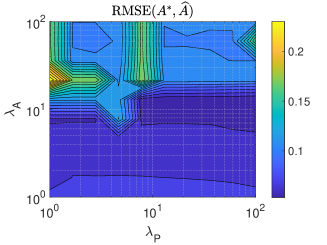
Refer to caption Refer to caption
Figure 4: Evolution of RMSE, F1, cNMSE and loss scores on the estimation of 𝐀𝐀{\mathbf{A}} (left) and 𝐏𝐏{\mathbf{P}} (right) by DGLASSO, as a function of hyperparameters (λA,λP)subscript𝜆𝐴subscript𝜆𝑃(\lambda_{A},\lambda_{P}), for dataset A (averaged on 10 runs). As a comparison, the averaged RMSE scores for (λA,λP)=(0,0)subscript𝜆𝐴subscript𝜆𝑃00(\lambda_{A},\lambda_{P})=(0,0) (i.e., MLEM) on this example were (0.077,0.106)0.0770.106(0.077,0.106) for (𝐀,𝐏)𝐀𝐏({\mathbf{A}},{\mathbf{P}}), respectively.

5.1.5 Influence of conditioning number

We report in Table 1 the results, averaged over 50 realizations of the time series generation. We do not provide the scores for the estimation of 𝐀𝐀{\mathbf{A}} (resp. (𝐏,𝐐)𝐏𝐐({\mathbf{P}},{\mathbf{Q}})) for GLASSO/rGLASSO (resp. GRAPHEM), as those methods are not designed for such task. The general trend in the results is a slight decrease of the quality of estimation for all methods, when cQsubscript𝑐𝑄c_{Q} increases (i.e., from dataset A to D). This is expected, as an ill-conditioned matrix 𝐐𝐐{\mathbf{Q}} complicates the mathematical structure of the likelihood term.

Regarding the estimation of 𝐀𝐀{\mathbf{A}}, GRAPHEM method presents the best results for the three considered metrics. DGLASSO is second best, while MLEM follows. As already stated, GLASSO/rGLASSO do not estimate 𝐀𝐀{\mathbf{A}} (i.e., they assume this matrix to be zero, that is the process is i.i.d. without any Markov structure). Regarding the estimation of (𝐏,𝐐)𝐏𝐐({\mathbf{P}},{\mathbf{Q}}), DGLASSO is outperforming the benchmarks in terms of RMSE score. The second best, in terms of RMSE is MLEM. GLASSO and rGLASSO gets very bad RMSE scores, probably because of the model mismatch induced by assuming 𝐀𝐀{\mathbf{A}} to be zero. The edge detection performance of DGLASSO are excellent, except in few cases where rGLASSO gets slightly better results. MLEM gets poorer results than DGLASSO in all metrics. In particular it exhibits a bad F1 score, as it does not include sparse prior, and thus does not succeed to eliminate any spurious edges.

Regarding the distribution mean calculation, it is remarkable that DGLASSO outperforms in all examples the benchmarks, which shows that the proposed formulation allows to provide model parameters that are best suited for inference using KF/RTS at test phase. The marginal likelihood log-loss is also minimized with the quantities provided by our method. This could appear as counter-intuitive, as the method is not specifically designed to minimize this loss (while MLEM is). The advantage of DGLASSO is that it accounts for prior knowledge, making the inferred model more robust, and less prone to overfitting, which is translated into better behavior on an independent test time series.

We display in Figure 5 box plots assessing the variability to the RMSE and F1 scores, for both MLEM and DGLASSO methods, on 50 runs on dataset A and dataset D. The RMSE values are in most runs lower (i.e., better) for the proposed method. Both methods are quite stable with respect to the time series generation, as the plots show few outliers. For dataset D, corresponding to a more challenging case with an ill-conditioned matrix 𝐏superscript𝐏{\mathbf{P}}^{*}, the results are slightly more spread, especially for the metrics related to the recovery quality of this matrix. Remark that the F1 scores of MLEM are constant, equal to 0.5. As already pointing out, this is expected as MLEM is not designed to perform an edge detection task.

We refer the reader to Appendix C.3 for extra experiments on the synthetic datasets, assessing the performance of DGLASSO when the sparsity level of 𝐀superscript𝐀{\mathbf{A}}^{*} increases.

Refer to caption Refer to caption
Figure 5: Box plots for the RMSE and F1 scores when running MLEM (left) and DGLASSO (right) on 50 randomly generated LG-SSM time series, for dataset A (top) and dataset D (bottom). DGLASSO outperforms MLEM on all runs, in terms of accuracy metrics (the higher, the better), while its RMSE scores are better (i.e., lower) for DGLASSO for most runs. Dataset D is more challenging, in terms of inference, thus yielding to more spread results for both methods.
Table 1: Results for the four considered datasets A to D, with an increasing conditioning number of 𝐏superscript𝐏{\mathbf{P}}^{*} equals to log10(c){0.1,0.2,0.1,1}subscript10𝑐0.10.20.11\log_{10}(c)\in\{0.1,0.2,0.1,1\}, respectively. We evaluate the methods in terms of estimation quality for (𝐀,𝐏,𝐐)𝐀𝐏𝐐({\mathbf{A}},{\mathbf{P}},{\mathbf{Q}}), using either RMSE as defined in (63), and edge detection scores (AUC, F1), as well as in terms of inference quality using cNMSE metrics defined in (64).
Estimation of 𝐀𝐀{\mathbf{A}} Estimation of 𝐏𝐏{\mathbf{P}} Estim. 𝐐𝐐{\mathbf{Q}} State distrib. Predictive distrib.
Method RMSE AUC F1 RMSE AUC F1 RMSE cNMSE(𝝁,𝝁^)superscript𝝁^𝝁(\bm{\mu}^{*},\widehat{\bm{\mu}}) cNMSE(𝝁s,𝝁^s)superscript𝝁ssuperscript^𝝁s(\bm{\mu}^{\text{s}*},\widehat{\bm{\mu}}^{\text{s}}) cNMSE(𝝂,𝝂^)superscript𝝂^𝝂({\bm{\nu}}^{*},\widehat{{\bm{\nu}}}) 1:K(𝐀^,𝐏^)subscript:1𝐾^𝐀^𝐏\mathcal{L}_{1:K}(\widehat{{\mathbf{A}}},\widehat{{\mathbf{P}}})
Dataset A DGLASSO 0.060 5250.0605250.060\,525 0.842 550.842550.842\,55 0.640 570.640570.640\,57 0.081 9270.0819270.081\,927 0.778 010.778010.778\,01 0.698 120.698120.698\,12 0.082 6010.0826010.082\,601 6.393 5×𝟏𝟎𝟎𝟖6.3935E-086.393\,5\text{\times}{10}^{-08} 1.050 4×𝟏𝟎𝟎𝟕1.0504E-071.050\,4\text{\times}{10}^{-07} 2.983 7×𝟏𝟎𝟒2.9837E-42.983\,7\text{\times}{10}^{-4} 12 307.168 712307.168712\,307.168\,7
MLEM 0.076 0630.0760630.076\,063 0.816 930.816930.816\,93 0.50.50.5 0.105 280.105280.105\,28 0.857 390.857390.857\,39 0.50.50.5 0.101 520.101520.101\,52 1.094 7×10071.0947E-071.094\,7\text{\times}{10}^{-07} 1.802 5×10071.8025E-071.802\,5\text{\times}{10}^{-07} 4.842 5×1044.8425E-44.842\,5\text{\times}{10}^{-4} 12 341.204 512341.204512\,341.204\,5
GLASSO NA NA NA 0.818 380.818380.818\,38 0.803 940.803940.803\,94 0.496 160.496160.496\,16 1 073.510 41073.51041\,073.510\,4 4.485 3×10064.4853E-064.485\,3\text{\times}{10}^{-06} 7.180 4×10067.1804E-067.180\,4\text{\times}{10}^{-06} 111 28 459.293 528459.293528\,459.293\,5
rGLASSO NA NA NA 0.763 760.763760.763\,76 0.923 770.923770.923\,77 0.597 590.597590.597\,59 31.689 131.689131.689\,1 2.825 6×10062.8256E-062.825\,6\text{\times}{10}^{-06} 5.492 4×10065.4924E-065.492\,4\text{\times}{10}^{-06} 111 22 957.692 822957.692822\,957.692\,8
GRAPHEM 0.044 6310.0446310.044\,631 0.894 810.894810.894\,81 0.846 540.846540.846\,54 NA NA NA NA 4.364 2×10064.3642E-064.364\,2\text{\times}{10}^{-06} 6.944 3×10066.9443E-066.944\,3\text{\times}{10}^{-06} 2.98×1042.98E-42.98\text{\times}{10}^{-4} 29 035.029 629035.029629\,035.029\,6
Dataset B DGLASSO 0.068 3310.0683310.068\,331 0.833 170.833170.833\,17 0.603 220.603220.603\,22 0.070 2990.0702990.070\,299 0.893 40.89340.893\,4 0.835 360.835360.835\,36 0.070 780.070780.070\,78 7.489 9×𝟏𝟎𝟎𝟖7.4899E-087.489\,9\text{\times}{10}^{-08} 1.236 1×𝟏𝟎𝟎𝟕1.2361E-071.236\,1\text{\times}{10}^{-07} 3.280 8×𝟏𝟎𝟒3.2808E-43.280\,8\text{\times}{10}^{-4} 11 806.743 911806.743911\,806.743\,9
MLEM 0.079 5440.0795440.079\,544 0.814 950.814950.814\,95 0.50.50.5 0.105 860.105860.105\,86 0.8980.8980.898 0.50.50.5 0.100 190.100190.100\,19 1.298 7×10071.2987E-071.298\,7\text{\times}{10}^{-07} 2.133 2×10072.1332E-072.133\,2\text{\times}{10}^{-07} 4.618 5×1044.6185E-44.618\,5\text{\times}{10}^{-4} 11 833.447 811833.447811\,833.447\,8
GLASSO NA NA NA 0.827 480.827480.827\,48 0.825 650.825650.825\,65 0.505 310.505310.505\,31 341.872 6341.8726341.872\,6 5.068 9×10065.0689E-065.068\,9\text{\times}{10}^{-06} 8.071 8×10068.0718E-068.071\,8\text{\times}{10}^{-06} 111 27 744.964 227744.964227\,744.964\,2
rGLASSO NA NA NA 0.733 850.733850.733\,85 0.930 290.930290.930\,29 0.607 940.607940.607\,94 33.895 533.895533.895\,5 3.214 5×10063.2145E-063.214\,5\text{\times}{10}^{-06} 6.186 6×10066.1866E-066.186\,6\text{\times}{10}^{-06} 111 22 530.036 322530.036322\,530.036\,3
GRAPHEM 0.046 7950.0467950.046\,795 0.893 390.893390.893\,39 0.847 790.847790.847\,79 NA NA NA NA 5.158 4×10065.1584E-065.158\,4\text{\times}{10}^{-06} 8.036 2×10068.0362E-068.036\,2\text{\times}{10}^{-06} 2.912 2×1042.9122E-42.912\,2\text{\times}{10}^{-4} 29 031.411 629031.411629\,031.411\,6
Dataset C DGLASSO 0.070 2270.0702270.070\,227 0.829 030.829030.829\,03 0.581 260.581260.581\,26 0.090 3610.0903610.090\,361 0.953 720.953720.953\,72 0.829 540.829540.829\,54 0.077 9050.0779050.077\,905 1.896 2×𝟏𝟎𝟎𝟕1.8962E-071.896\,2\text{\times}{10}^{-07} 2.994 1×𝟏𝟎𝟎𝟕2.9941E-072.994\,1\text{\times}{10}^{-07} 3.955 6×𝟏𝟎𝟒3.9556E-43.955\,6\text{\times}{10}^{-4} 10 311.10410311.10410\,311.104
MLEM 0.081 2040.0812040.081\,204 0.810 250.810250.810\,25 0.50.50.5 0.097 3570.0973570.097\,357 0.973 610.973610.973\,61 0.50.50.5 0.094 3660.0943660.094\,366 2.582 7×10072.5827E-072.582\,7\text{\times}{10}^{-07} 4.179 6×10074.1796E-074.179\,6\text{\times}{10}^{-07} 5.052 6×1045.0526E-45.052\,6\text{\times}{10}^{-4} 10 326.409 910326.409910\,326.409\,9
GLASSO NA NA NA 0.901 320.901320.901\,32 0.804 980.804980.804\,98 0.489 250.489250.489\,25 3.926×10173.926E+173.926\text{\times}{10}^{17} 0.012 0270.0120270.012\,027 0.012 0320.0120320.012\,032 111 26 634.891 726634.891726\,634.891\,7
rGLASSO NA NA NA 0.805 170.805170.805\,17 0.927 810.927810.927\,81 0.614 210.614210.614\,21 29.530 229.530229.530\,2 7.194 8×10067.1948E-067.194\,8\text{\times}{10}^{-06} 1.319 5×10051.3195E-051.319\,5\text{\times}{10}^{-05} 111 21 322.246 521322.246521\,322.246\,5
GRAPHEM 0.049 2760.0492760.049\,276 0.891 850.891850.891\,85 0.8570.8570.857 NA NA NA NA 1.054 8×10051.0548E-051.054\,8\text{\times}{10}^{-05} 1.640 5×10051.6405E-051.640\,5\text{\times}{10}^{-05} 3.912 1×1043.9121E-43.912\,1\text{\times}{10}^{-4} 29 023.36929023.36929\,023.369
Dataset D DGLASSO 0.073 4610.0734610.073\,461 0.835 140.835140.835\,14 0.574 520.574520.574\,52 0.083 3770.0833770.083\,377 𝟏11 0.598 280.598280.598\,28 0.080 4250.0804250.080\,425 5.127 2×𝟏𝟎𝟎𝟕5.1272E-075.127\,2\text{\times}{10}^{-07} 8.243 4×𝟏𝟎𝟎𝟕8.2434E-078.243\,4\text{\times}{10}^{-07} 3.372 9×𝟏𝟎𝟒3.3729E-43.372\,9\text{\times}{10}^{-4} 7 911.943 17911.94317\,911.943\,1
MLEM 0.097 630.097630.097\,63 0.808 190.808190.808\,19 0.50.50.5 0.094 5630.0945630.094\,563 𝟏11 0.50.50.5 0.083 5010.0835010.083\,501 6.295 6×10076.2956E-076.295\,6\text{\times}{10}^{-07} 1.026 6×10061.0266E-061.026\,6\text{\times}{10}^{-06} 4.218 8×1044.2188E-44.218\,8\text{\times}{10}^{-4} 7 923.849 97923.84997\,923.849\,9
GLASSO NA NA NA 0.964 140.964140.964\,14 0.940 640.940640.940\,64 0.550 360.550360.550\,36 187.822 7187.8227187.822\,7 2.347 8×10052.3478E-052.347\,8\text{\times}{10}^{-05} 3.701 2×10053.7012E-053.701\,2\text{\times}{10}^{-05} 111 23 684.177 823684.177823\,684.177\,8
rGLASSO NA NA NA 0.881 820.881820.881\,82 0.956 090.956090.956\,09 0.645 090.645090.645\,09 28.702 728.702728.702\,7 1.886 4×10051.8864E-051.886\,4\text{\times}{10}^{-05} 3.239 1×10053.2391E-053.239\,1\text{\times}{10}^{-05} 111 20 100.49120100.49120\,100.491
GRAPHEM 0.060 6150.0606150.060\,615 0.891 70.89170.891\,7 0.864 380.864380.864\,38 NA NA NA NA 2.503×10052.503E-052.503\text{\times}{10}^{-05} 3.838 8×10053.8388E-053.838\,8\text{\times}{10}^{-05} 3.743 1×1043.7431E-43.743\,1\text{\times}{10}^{-4} 29 016.320 929016.320929\,016.320\,9

5.1.6 Complexity analysis

We now examine the time complexity of the method, as well as of MLEM, when processing dataset A, for various values of the time series length K𝐾K, namely K{100,200,500,1000,2000,5000}𝐾100200500100020005000K\in\{100,200,500,1000,2000,5000\} (we recall that our previous experiments were all done with K=1000𝐾1000K=1000). We display in Figure 6(left) the computing time in seconds for computing (𝐀^,𝐏^)^𝐀^𝐏(\widehat{{\mathbf{A}}},\widehat{{\mathbf{P}}}), for DGLASSO and MLEM, averaged over 50 realizations. We also display, in Figure 6(middle) for the same experiment, the RMSE between 𝐀superscript𝐀{\mathbf{A}}^{*} and 𝐀^^𝐀\widehat{{\mathbf{A}}}, and in Figure 6(right) the metric cNMSE(𝝁,𝝁^)cNMSEsuperscript𝝁^𝝁\text{cNMSE}(\bm{\mu}^{*},\widehat{\bm{\mu}}). One can notice that our method is slightly more demanding in terms of computational time, but it scales similarly than its non regularized version MLEM. Moreover, as already observed in our previous experiments, DGLASSO outperforms MLEM on both metrics shown here, in all tested values of K𝐾K. As expected, the results are better for higher values of K𝐾K, at the price of an increased computational time. Interestingly, the regularization still yields improved results for very large K𝐾K.

Refer to caption Refer to caption Refer to caption
Figure 6: Evolution of the complexity time (left), RMSE(𝐀,𝐀^)superscript𝐀^𝐀({\mathbf{A}}^{*},\widehat{{\mathbf{A}}}) (middle) and cNMSE(𝝁,𝝁^)cNMSEsuperscript𝝁^𝝁\text{cNMSE}(\bm{\mu}^{*},\widehat{\bm{\mu}}) (right) metrics, as a function of the time series length K𝐾K, for experiments on dataset A averaged over 50 runs.

5.2 Weather data

5.2.1 Experimental settings

We now evaluate our method on realistic graph datasets arising from causal discovery studies in the field of weather variability tracking. Specifically, we consider two sets of 200200200 sparse matrices 𝐀Nxsuperscript𝐀superscriptsubscript𝑁𝑥{\mathbf{A}}^{*}\in\mathbb{R}^{N_{x}}, with Nx=5subscript𝑁𝑥5N_{x}=5 or 101010 respectively, representing the ground truth causal graphs used to produce WEATH datasets in the Neurips 2019 data challenge (Runge et al., 2020)555https://causeme.uv.es/static/datasets/TestWEATH/. For each 𝐀superscript𝐀{\mathbf{A}}^{*}, we create times series (𝐱k,𝐲k)k=1Ksuperscriptsubscriptsubscript𝐱𝑘subscript𝐲𝑘𝑘1𝐾({\mathbf{x}}_{k},{\mathbf{y}}_{k})_{k=1}^{K} using (2)-(3), with K=103𝐾superscript103K=10^{3}, 𝐇=Idsuperscript𝐇Id{\mathbf{H}}^{*}={\textbf{Id}} (i.e., Ny=Nxsubscript𝑁𝑦subscript𝑁𝑥N_{y}=N_{x}), and (σ𝐑,σ0)=(101,104)subscript𝜎𝐑subscript𝜎0superscript101superscript104(\sigma_{{\mathbf{R}}},\sigma_{0})=(10^{-1},10^{-4}). We set 𝐐superscript𝐐{\mathbf{Q}}^{*} as a block diagonal matrix of J𝐽J blocks with dimensions Bj1jJsubscriptsubscript𝐵𝑗1𝑗𝐽{B_{j}}_{1\leq j\leq J}, with j=1JBj=Nxsuperscriptsubscript𝑗1𝐽subscript𝐵𝑗subscript𝑁𝑥\sum_{j=1}^{J}B_{j}=N_{x}. Here, we consider two settings for the conditioning of 𝐐superscript𝐐{\mathbf{Q}}^{*}, namely one with a condition number close to one (i.e., 𝐐superscript𝐐{\mathbf{Q}}^{*} is close to identity matrix) and another with high condition number. The main characteristics of the datasets and their names are summarized in Table 2.

We evaluate our results in terms on quality assessment metrics of the estimated 𝐀^^𝐀\widehat{{\mathbf{A}}} when compared to its ground truth 𝐀superscript𝐀{\mathbf{A}}^{*}, as this is the quantity of interest for these datasets. We compute RMSE(𝐀^,𝐀)^𝐀superscript𝐀(\widehat{{\mathbf{A}}},{\mathbf{A}}^{*}), as well as the precision, recall, specificity, accuracy, and F1 score for detecting the non-zero entries of the transition matrix (that is, the graph edges positions). A threshold value of 1010superscript101010^{-10} on the absolute entries is used for the detection hypothesis.

As for comparison, we also provide the results obtained with MLEM and GRAPHEM approaches, as in our previous experiments. The same stopping criterion than in our previous set of experiments is used. The hyperparameters are finetuned using the strategy depicted on the previous section. We used rough grids for the finetuning and keep the parameters fixed for all the dataset, to avoid any overfitting behavior. In addition to these EM-based methods, we provide comparisons with two Granger-causality approaches for graphical modeling, namely pairwise Granger Causality (PGC) and conditional Granger Causality (CGC). Those approaches are based on sparse vector autoregressive (VAR) models. We allow the order of the VAR process to be up to p=11𝑝11p=11, CGC is run with a maximum distance of 555 causal links, and in each experiment we display the best results (in F1 score) for the statistical tests performed with the significance level α{0.01,0.05,0.1}𝛼0.010.050.1\alpha\in\{0.01,0.05,0.1\} (see more details in (Luengo et al., 2019)). As PGC and CGC do not provide a weighted graph estimation, no RMSE score is computed in those cases.

5.2.2 Results

We summarize our results in Table 3. We also report the averaged inference time for all methods. Remarkably, the proposed method outperforms all benchmarks in all the considered metrics, related to the inference of the graph weights (RMSE metric) and the edge detection task (binary classification metrics). As expected, the result quality tends to slightly degrade when a more complicated structure is assumed for 𝐐superscript𝐐{\mathbf{Q}}^{*} (see, for instance, WeathN5a versus WeathN5b), and when the dataset size increases (see, for instance, WeathN5a versus WeathN10a). MLEM has very poor edge detection metrics, since it does not exploit any sparsity prior on the sought matrix. GRAPHEM has better behavior, but, in these datasets, it stays way behind the quality of DGLASSO, by all metrics (which was not the case for the synthetic data). This shows that our method really makes the change when dealing with complex graphs and correlated noise in the observations. In terms of computational time, the proposed method has similar complexity than the two other EM-based approaches. The results of CGC and PGC are satisfactory in the first two examples although the binary metrics are far from the performance of DGLASSO. PGC still gives meaningful results in the last two examples, but CGC has a low performance due to a high number of false negatives (i.e., many existing links are not discovered). We also note that while PGC and CGC have significantly lower running times for the case with Ny=5subscript𝑁𝑦5N_{y}=5, the computational cost for Ny=10subscript𝑁𝑦10N_{y}=10 is closer to DGLASSO while the performance gap is higher. Thus, in this examples we show that as the dimension grows, the computational cost of all methods is comparable while the proposed method has clearly a better performance. We also display some examples of inferred graphs in Figures 7 and 8. We can observe that DGLASSO is able to capture in a very accurate manner the structure of the graphs, despite the wide variability of the dataset. MLEM and GRAPHEM capture the main edges, but their graphs are perturbed by several spurious edges, which shows how important it is to adopt a joint graph modeling, with sparsity priors on each.

Dataset Nx=Nysubscript𝑁𝑥subscript𝑁𝑦N_{x}=N_{y} (Bj)1jJsubscriptsubscript𝐵𝑗1𝑗𝐽(B_{j})_{1\leq j\leq J} log10(cond(𝐐))subscript10condsuperscript𝐐\log_{10}(\text{cond}({\mathbf{Q}}^{*}))
WeathN5a 555 (2,3)23(2,3) 0.10.10.1
WeathN5b 555 (2,3)23(2,3) 111
WeathN10a 101010 (5,5)55(5,5) 0.10.10.1
WeathN10b 101010 (5,5)55(5,5) 111
Table 2: Details about the datasets. Each dataset is associated with 200200200 examples for matrix 𝐀superscript𝐀{\mathbf{A}}^{*}.
Table 3: Results for climate datasets along with computing times. All the metrics are averaged over the 200200200 examples of the dataset.
method RMSE accur. prec. recall spec. F1 Time (s.)
WeathN5a DGLASSO 0.107 540.107540.107\,54 0.937 40.93740.937\,4 0.894 220.894220.894\,22 0.998 140.998140.998\,14 0.894 020.894020.894\,02 0.937 450.937450.937\,45 0.607 790.607790.607\,79
MLEM 0.139 740.139740.139\,74 0.412 80.41280.412\,8 0.412 80.41280.412\,8 𝟏11 00 0.584 040.584040.584\,04 0.595 860.595860.595\,86
GRAPHEM 0.126 60.12660.126\,6 0.703 40.70340.703\,4 0.595 240.595240.595\,24 𝟏11 0.495 830.495830.495\,83 0.741 50.74150.741\,5 0.605 810.605810.605\,81
PGC - 0.772 40.77240.772\,4 0.902 070.902070.902\,07 0.514 930.514930.514\,93 0.952 620.952620.952\,62 0.652 20.65220.652\,2 0.018 7220.0187220.018\,722
CGC - 0.672 40.67240.672\,4 0.827 890.827890.827\,89 0.284 570.284570.284\,57 0.944 850.944850.944\,85 0.414 570.414570.414\,57 0.025 6290.0256290.025\,629
WeathN5b DGLASSO 0.165 890.165890.165\,89 0.772 80.77280.772\,8 0.667 510.667510.667\,51 0.991 910.991910.991\,91 0.619 460.619460.619\,46 0.787 980.787980.787\,98 0.629 550.629550.629\,55
MLEM 0.197 220.197220.197\,22 0.412 80.41280.412\,8 0.412 80.41280.412\,8 𝟏11 00 0.584 040.584040.584\,04 0.375 520.375520.375\,52
GRAPHEM 0.185 820.185820.185\,82 0.6290.6290.629 0.535 710.535710.535\,71 𝟏11 0.368 330.368330.368\,33 0.694 460.694460.694\,46 0.469 60.46960.469\,6
PGC - 0.675 20.67520.675\,2 0.677 350.677350.677\,35 0.469 330.469330.469\,33 0.818 970.818970.818\,97 0.544 320.544320.544\,32 0.016 8510.0168510.016\,851
CGC - 0.6340.6340.634 0.658 770.658770.658\,77 0.262 710.262710.262\,71 0.895 010.895010.895\,01 0.369 080.369080.369\,08 0.023 1020.0231020.023\,102
WeathN10a DGLASSO 0.201 950.201950.201\,95 0.9480.9480.948 0.898 480.898480.898\,48 0.925 430.925430.925\,43 0.954 120.954120.954\,12 0.890 220.890220.890\,22 1.363 41.36341.363\,4
MLEM 0.264 380.264380.264\,38 0.219 150.219150.219\,15 0.219 150.219150.219\,15 𝟏11 00 0.3590.3590.359 0.833 960.833960.833\,96
GRAPHEM 0.224 30.22430.224\,3 0.510 950.510950.510\,95 0.311 130.311130.311\,13 0.999 790.999790.999\,79 0.373 860.373860.373\,86 0.473 330.473330.473\,33 1.444 91.44491.444\,9
PGC - 0.878 60.87860.878\,6 0.904 20.90420.904\,2 0.504 160.504160.504\,16 0.983 460.983460.983\,46 0.643 80.64380.643\,8 0.232 040.232040.232\,04
CGC - 0.773 250.773250.773\,25 0.539 470.539470.539\,47 0.210 570.210570.210\,57 0.931 920.931920.931\,92 0.278 020.278020.278\,02 0.357 70.35770.357\,7
WeathN10b DGLASSO 0.192 220.192220.192\,22 0.865 850.865850.865\,85 0.633 40.63340.633\,4 0.994 40.99440.994\,4 0.829 30.82930.829\,3 0.769 150.769150.769\,15 0.556 890.556890.556\,89
MLEM 0.342 080.342080.342\,08 0.219 150.219150.219\,15 0.219 150.219150.219\,15 𝟏11 00 0.3590.3590.359 0.988 910.988910.988\,91
GRAPHEM 0.219 360.219360.219\,36 0.854 50.85450.854\,5 0.619 830.619830.619\,83 0.994 040.994040.994\,04 0.815 520.815520.815\,52 0.757 180.757180.757\,18 0.655 450.655450.655\,45
PGC - 0.798 70.79870.798\,7 0.558 290.558290.558\,29 0.473 250.473250.473\,25 0.889 880.889880.889\,88 0.506 040.506040.506\,04 0.153 7570.1537570.153\,757
CGC - 0.750 350.750350.750\,35 0.406 680.406680.406\,68 0.217 620.217620.217\,62 0.900 20.90020.900\,2 0.264 620.264620.264\,62 0.178 460.178460.178\,46
Refer to caption Refer to caption Refer to caption Refer to caption
Figure 7: Graph inference results on 444 examples extracted from the dataset WeathN5a. From top to bottom: Original graph representation of 𝐀superscript𝐀{\mathbf{A}}^{*}, and of its estimation 𝐀^^𝐀\widehat{{\mathbf{A}}}, using DGLASSO, MLEM, GRAPHEM, respectively.
Refer to caption Refer to caption Refer to caption Refer to caption
Figure 8: Graph inference results on 444 examples extracted from the dataset WeathN10a. From top to bottom: Original graph representation of 𝐀superscript𝐀{\mathbf{A}}^{*}, and of its estimation 𝐀^^𝐀\widehat{{\mathbf{A}}}, using DGLASSO, MLEM, GRAPHEM, respectively.

6 Conclusion

This paper proposes a joint graphical modeling approach that incorporates a graphical perspective on the dynamics of the hidden state of a linear Gaussian state-space model. In particular, we propose a joint approach that considers a sparse undirected graph as a prior on the precision matrix of the hidden state noise and a sparse directed graph for the transition matrix that models the state dynamics. By bridging the gap between the static graphical Lasso model and the dynamic state-space model, we provide a novel comprehensive framework for interpretable inference with time-series data. The presented inference method, based on an efficient block alternating majorization-minimization algorithm, enables simultaneous estimation of both graphs and the construction of the filtering/smoothing distribution for the time series. The established convergence of our algorithm, departing from recent nonlinear analysis tools, enhances the reliability and practicality of our approach. Through extensive experimental validation on synthetic and real weather variability data, we have demonstrated the effectiveness and potential of our proposed model and inference algorithm. The results showcase its ability to uncover meaningful insights from time-series data, contributing not only to better forecasting performance but also to a better understanding of complex phenomena in various scientific and engineering domains. Future research can further explore and extend the presented framework to tackle even more challenging state-space models, and more complex graphical structures.


Acknowledgments

É.C. acknowledges support from the European Research Council Starting Grant MAJORIS ERC-2019-STG-850925. The work of V. E. is supported by the Agence Nationale de la Recherche of France under PISCES (ANR-17-CE40-0031-01), the Leverhulme Research Fellowship (RF-2021-593), and by ARL/ARO under grant W911NF-22-1-0235.
The authors thank Gustau Camps-Valls and his team, for providing the ground truth data for (Runge et al., 2020).

Appendix A Proof of Theorem 1

For any initial state 𝐱0:Ksubscript𝐱:0𝐾{\mathbf{x}}_{0:K}, with non zero probability, the neg-log-likelihood (𝐀,𝐏)(1:K(𝐀,𝐏)=logp(𝐲1:K|𝐀,𝐏))𝐀𝐏subscript:1𝐾𝐀𝐏𝑝conditionalsubscript𝐲:1𝐾𝐀𝐏({\mathbf{A}},{\mathbf{P}})\to\left(\mathcal{L}_{1:K}({\mathbf{A}},{\mathbf{P}})=-\log p({\mathbf{y}}_{1:K}|{\mathbf{A}},{\mathbf{P}})\right) reads, according to Bayes’ rule,

(𝐀Nx×Nx)(𝐏𝒮Nx)1:K(𝐀,𝐏)=logp(𝐱0:K,𝐲1:K|𝐀,𝐏)+logp(𝐱0:K|𝐲1:K,𝐀,𝐏).for-all𝐀superscriptsubscript𝑁𝑥subscript𝑁𝑥for-all𝐏subscript𝒮subscript𝑁𝑥subscript:1𝐾𝐀𝐏𝑝subscript𝐱:0𝐾conditionalsubscript𝐲:1𝐾𝐀𝐏𝑝conditionalsubscript𝐱:0𝐾subscript𝐲:1𝐾𝐀𝐏(\forall{\mathbf{A}}\in\mathbb{R}^{N_{x}\times N_{x}})(\forall{\mathbf{P}}\in\mathcal{S}_{N_{x}})\\ \mathcal{L}_{1:K}({\mathbf{A}},{\mathbf{P}})=-\log p({\mathbf{x}}_{0:K},{\mathbf{y}}_{1:K}|{\mathbf{A}},{\mathbf{P}})+\log p({\mathbf{x}}_{0:K}|{\mathbf{y}}_{1:K},{\mathbf{A}},{\mathbf{P}}). (65)

According to Eqs. (2)-(3)

logp(𝐱0:K,𝐲1:K|𝐀,𝐏)=logp(𝐱0)+k=1Klogp(𝐱k|𝐱k1,𝐀,𝐏)+k=1Klogp(𝐲k|𝐱k).𝑝subscript𝐱:0𝐾conditionalsubscript𝐲:1𝐾𝐀𝐏𝑝subscript𝐱0superscriptsubscript𝑘1𝐾𝑝conditionalsubscript𝐱𝑘subscript𝐱𝑘1𝐀𝐏superscriptsubscript𝑘1𝐾𝑝conditionalsubscript𝐲𝑘subscript𝐱𝑘\log p({\mathbf{x}}_{0:K},{\mathbf{y}}_{1:K}|{\mathbf{A}},{\mathbf{P}})=\log p({\mathbf{x}}_{0})+\sum_{k=1}^{K}\log p({\mathbf{x}}_{k}|{\mathbf{x}}_{k-1},{\mathbf{A}},{\mathbf{P}})+\sum_{k=1}^{K}\log p({\mathbf{y}}_{k}|{\mathbf{x}}_{k}). (66)

Moreover, using again Eq. (2) and the statistical model of the state noise,

(𝐀Nx×Nx)for-all𝐀superscriptsubscript𝑁𝑥subscript𝑁𝑥\displaystyle(\forall{\mathbf{A}}\in\mathbb{R}^{N_{x}\times N_{x}}) (𝐏𝒮Nx)for-all𝐏subscript𝒮subscript𝑁𝑥\displaystyle(\forall{\mathbf{P}}\in\mathcal{S}_{N_{x}}) (67)
k=1Klogp(𝐱k|𝐱k1,𝐀,𝐏)superscriptsubscript𝑘1𝐾𝑝conditionalsubscript𝐱𝑘subscript𝐱𝑘1𝐀𝐏\displaystyle\sum_{k=1}^{K}\log p({\mathbf{x}}_{k}|{\mathbf{x}}_{k-1},{\mathbf{A}},{\mathbf{P}}) =12k=1K((𝐱k𝐀𝐱k1)𝐏(𝐱k𝐀𝐱k1)logdet(2π𝐏)),absent12superscriptsubscript𝑘1𝐾superscriptsubscript𝐱𝑘subscript𝐀𝐱𝑘1top𝐏subscript𝐱𝑘subscript𝐀𝐱𝑘12𝜋𝐏\displaystyle=-\frac{{1}}{2}\sum_{k=1}^{K}\left(\left({\mathbf{x}}_{k}-{\mathbf{A}}{\mathbf{x}}_{k-1}\right)^{\top}{\mathbf{P}}\left({\mathbf{x}}_{k}-{\mathbf{A}}{\mathbf{x}}_{k-1}\right)-\log\det({2\pi}{{\mathbf{P}}})\right), (68)
=12k=1K((𝐱k𝐀𝐱k1)𝐏(𝐱k𝐀𝐱k1))+K2logdet(2π𝐏),absent12superscriptsubscript𝑘1𝐾superscriptsubscript𝐱𝑘subscript𝐀𝐱𝑘1top𝐏subscript𝐱𝑘subscript𝐀𝐱𝑘1𝐾22𝜋𝐏\displaystyle=-\frac{{1}}{2}\sum_{k=1}^{K}\left(\left({\mathbf{x}}_{k}-{\mathbf{A}}{\mathbf{x}}_{k-1}\right)^{\top}{\mathbf{P}}\left({\mathbf{x}}_{k}-{\mathbf{A}}{\mathbf{x}}_{k-1}\right)\right)+\frac{K}{2}\log\det({2\pi}{{\mathbf{P}}}), (69)

which concludes the first part of the proof.
Let us now consider some 𝐀~Nx×Nx~𝐀superscriptsubscript𝑁𝑥subscript𝑁𝑥\widetilde{{\mathbf{A}}}\in\mathbb{R}^{N_{x}\times N_{x}} and 𝐏~𝒮Nx++~𝐏superscriptsubscript𝒮subscript𝑁𝑥absent\widetilde{{\mathbf{P}}}\in\mathcal{S}_{N_{x}}^{++}. We start by recalling some known results arising from the EM methodology (Dempster et al., 1977; Wu, 1983), that we specify here for our context for the sake of clarity. First, we notice that

(𝐀Nx×Nx)(𝐏𝒮Nx)1:K(𝐀,𝐏)=logp(𝐲1:K|𝐀,𝐏)p(𝐱0:K|𝐲1:K,𝐀~,𝐏~)d𝐱0:K,for-all𝐀superscriptsubscript𝑁𝑥subscript𝑁𝑥for-all𝐏subscript𝒮subscript𝑁𝑥subscript:1𝐾𝐀𝐏𝑝conditionalsubscript𝐲:1𝐾𝐀𝐏𝑝conditionalsubscript𝐱:0𝐾subscript𝐲:1𝐾~𝐀~𝐏differential-dsubscript𝐱:0K(\forall{\mathbf{A}}\in\mathbb{R}^{N_{x}\times N_{x}})(\forall{\mathbf{P}}\in\mathcal{S}_{N_{x}})\\ \mathcal{L}_{1:K}({\mathbf{A}},{\mathbf{P}})=-\int\log p({\mathbf{y}}_{1:K}|{\mathbf{A}},{\mathbf{P}})p({\mathbf{x}}_{0:K}|{\mathbf{y}}_{1:K},\widetilde{{\mathbf{A}}},\widetilde{{\mathbf{P}}})\rm{d}{\mathbf{x}}_{0:K}, (70)

since logp(𝐲1:K|𝐀,𝐏)𝑝conditionalsubscript𝐲:1𝐾𝐀𝐏\log p({\mathbf{y}}_{1:K}|{\mathbf{A}},{\mathbf{P}}) is constant with respect to the integration variable, and the distribution p(𝐱0:K|𝐲1:K,𝐀~,𝐏~)𝑝conditionalsubscript𝐱:0𝐾subscript𝐲:1𝐾~𝐀~𝐏p({\mathbf{x}}_{0:K}|{\mathbf{y}}_{1:K},\widetilde{{\mathbf{A}}},\widetilde{{\mathbf{P}}}) integrates to one. Then, according to (65) and (70), the expectation of the neg-log-likelihood multiplied by p(𝐱0:K|𝐲1:K,𝐀~,𝐏~)𝑝conditionalsubscript𝐱:0𝐾subscript𝐲:1𝐾~𝐀~𝐏p({\mathbf{x}}_{0:K}|{\mathbf{y}}_{1:K},\widetilde{{\mathbf{A}}},\widetilde{{\mathbf{P}}}) over all possible values of the unknown state reads:

(𝐀Nx×Nx)(𝐏𝒮Nx)1:K(𝐀,𝐏)=p(𝐱0:K|𝐲1:K,𝐀~,𝐏~)logp(𝐱0:K,𝐲1:K|𝐀,𝐏)d𝐱0:Kq(𝐀,𝐏;𝐀~,𝐏~)+p(𝐱0:K|𝐲1:K,𝐀~,𝐏~)logp(𝐱0:K|𝐲1:K,𝐀,𝐏)d𝐱0:Kh(𝐀,𝐏;𝐀~,𝐏~).for-all𝐀superscriptsubscript𝑁𝑥subscript𝑁𝑥for-all𝐏subscript𝒮subscript𝑁𝑥subscript:1𝐾𝐀𝐏superscript𝑝conditionalsubscript𝐱:0𝐾subscript𝐲:1𝐾~𝐀~𝐏𝑝subscript𝐱:0𝐾conditionalsubscript𝐲:1𝐾𝐀𝐏differential-dsubscript𝐱:0K𝑞𝐀𝐏~𝐀~𝐏superscript𝑝conditionalsubscript𝐱:0𝐾subscript𝐲:1𝐾~𝐀~𝐏𝑝conditionalsubscript𝐱:0𝐾subscript𝐲:1𝐾𝐀𝐏differential-dsubscript𝐱:0K𝐀𝐏~𝐀~𝐏(\forall{\mathbf{A}}\in\mathbb{R}^{N_{x}\times N_{x}})(\forall{\mathbf{P}}\in\mathcal{S}_{N_{x}})\quad\mathcal{L}_{1:K}({\mathbf{A}},{\mathbf{P}})=\overbrace{-\int p({\mathbf{x}}_{0:K}|{\mathbf{y}}_{1:K},\widetilde{{\mathbf{A}}},\widetilde{{\mathbf{P}}})\log p({\mathbf{x}}_{0:K},{\mathbf{y}}_{1:K}|{\mathbf{A}},{\mathbf{P}})\rm{d}{\mathbf{x}}_{0:K}}^{q({\mathbf{A}},{\mathbf{P}};\widetilde{{\mathbf{A}}},\widetilde{{\mathbf{P}}})}\\ +\overbrace{\int p({\mathbf{x}}_{0:K}|{\mathbf{y}}_{1:K},\widetilde{{\mathbf{A}}},\widetilde{{\mathbf{P}}})\log p({\mathbf{x}}_{0:K}|{\mathbf{y}}_{1:K},{\mathbf{A}},{\mathbf{P}})\rm{d}{\mathbf{x}}_{0:K}}^{h({\mathbf{A}},{\mathbf{P}};\widetilde{{\mathbf{A}}},\widetilde{{\mathbf{P}}})}. (71)

In particular, for (𝐀,𝐏)=(𝐀~,𝐏~)𝐀𝐏~𝐀~𝐏({\mathbf{A}},{\mathbf{P}})=(\widetilde{{\mathbf{A}}},\widetilde{{\mathbf{P}}}), 1:K(𝐀~,𝐏~)=q(𝐀~,𝐏~;𝐀~,𝐏~)+h(𝐀~,𝐏~;𝐀~,𝐏~)subscript:1𝐾~𝐀~𝐏𝑞~𝐀~𝐏~𝐀~𝐏~𝐀~𝐏~𝐀~𝐏\mathcal{L}_{1:K}(\widetilde{{\mathbf{A}}},\widetilde{{\mathbf{P}}})=q(\widetilde{{\mathbf{A}}},\widetilde{{\mathbf{P}}};\widetilde{{\mathbf{A}}},\widetilde{{\mathbf{P}}})+h(\widetilde{{\mathbf{A}}},\widetilde{{\mathbf{P}}};\widetilde{{\mathbf{A}}},\widetilde{{\mathbf{P}}}) so that

(𝐀Nx×Nx)(𝐏𝒮Nx)1:K(𝐀,𝐏)1:K(𝐀~,𝐏~)=q(𝐀,𝐏;𝐀~,𝐏~)q(𝐀~,𝐏~;𝐀~,𝐏~)+h(𝐀,𝐏;𝐀~,𝐏~)h(𝐀~,𝐏~;𝐀~,𝐏~).for-all𝐀superscriptsubscript𝑁𝑥subscript𝑁𝑥for-all𝐏subscript𝒮subscript𝑁𝑥subscript:1𝐾𝐀𝐏subscript:1𝐾~𝐀~𝐏𝑞𝐀𝐏~𝐀~𝐏𝑞~𝐀~𝐏~𝐀~𝐏𝐀𝐏~𝐀~𝐏~𝐀~𝐏~𝐀~𝐏(\forall{\mathbf{A}}\in\mathbb{R}^{N_{x}\times N_{x}})(\forall{\mathbf{P}}\in\mathcal{S}_{N_{x}})\quad\mathcal{L}_{1:K}({\mathbf{A}},{\mathbf{P}})-\mathcal{L}_{1:K}(\widetilde{{\mathbf{A}}},\widetilde{{\mathbf{P}}})=q({\mathbf{A}},{\mathbf{P}};\widetilde{{\mathbf{A}}},\widetilde{{\mathbf{P}}})-q(\widetilde{{\mathbf{A}}},\widetilde{{\mathbf{P}}};\widetilde{{\mathbf{A}}},\widetilde{{\mathbf{P}}})\\ +h({\mathbf{A}},{\mathbf{P}};\widetilde{{\mathbf{A}}},\widetilde{{\mathbf{P}}})-h(\widetilde{{\mathbf{A}}},\widetilde{{\mathbf{P}}};\widetilde{{\mathbf{A}}},\widetilde{{\mathbf{P}}}). (72)

Using Gibbs’s inequality, h(𝐀,𝐏;𝐀~,𝐏~)h(𝐀~,𝐏~;𝐀~,𝐏~)𝐀𝐏~𝐀~𝐏~𝐀~𝐏~𝐀~𝐏h({\mathbf{A}},{\mathbf{P}};\widetilde{{\mathbf{A}}},\widetilde{{\mathbf{P}}})\leq h(\widetilde{{\mathbf{A}}},\widetilde{{\mathbf{P}}};\widetilde{{\mathbf{A}}},\widetilde{{\mathbf{P}}}), with equality at (𝐀,𝐏)=(𝐀~,𝐏~)𝐀𝐏~𝐀~𝐏({\mathbf{A}},{\mathbf{P}})=(\widetilde{{\mathbf{A}}},\widetilde{{\mathbf{P}}}). Thus, using (72), that is

(𝐀Nx×Nx)(𝐏𝒮Nx)1:K(𝐀,𝐏)q(𝐀,𝐏;𝐀~,𝐏~)+1:K(𝐀~,𝐏~)q(𝐀~,𝐏~;𝐀~,𝐏~),for-all𝐀superscriptsubscript𝑁𝑥subscript𝑁𝑥for-all𝐏subscript𝒮subscript𝑁𝑥subscript:1𝐾𝐀𝐏𝑞𝐀𝐏~𝐀~𝐏subscript:1𝐾~𝐀~𝐏𝑞~𝐀~𝐏~𝐀~𝐏(\forall{\mathbf{A}}\in\mathbb{R}^{N_{x}\times N_{x}})(\forall{\mathbf{P}}\in\mathcal{S}_{N_{x}})\quad\mathcal{L}_{1:K}({\mathbf{A}},{\mathbf{P}})\leq q({\mathbf{A}},{\mathbf{P}};\widetilde{{\mathbf{A}}},\widetilde{{\mathbf{P}}})+\mathcal{L}_{1:K}(\widetilde{{\mathbf{A}}},\widetilde{{\mathbf{P}}})-q(\widetilde{{\mathbf{A}}},\widetilde{{\mathbf{P}}};\widetilde{{\mathbf{A}}},\widetilde{{\mathbf{P}}}), (73)

where equality holds at (𝐀,𝐏)=(𝐀~,𝐏~)𝐀𝐏~𝐀~𝐏({\mathbf{A}},{\mathbf{P}})=(\widetilde{{\mathbf{A}}},\widetilde{{\mathbf{P}}}). Notice that, for any function reading

(𝐀Nx×Nx)(𝐏𝒮Nx)𝒬(𝐀,𝐏;𝐀~,𝐏~)=q(𝐀,𝐏;𝐀~,𝐏~)+ct/𝐀,𝐏,for-all𝐀superscriptsubscript𝑁𝑥subscript𝑁𝑥for-all𝐏subscript𝒮subscript𝑁𝑥𝒬𝐀𝐏~𝐀~𝐏𝑞𝐀𝐏~𝐀~𝐏subscriptctabsent𝐀𝐏(\forall{\mathbf{A}}\in\mathbb{R}^{N_{x}\times N_{x}})(\forall{\mathbf{P}}\in\mathcal{S}_{N_{x}})\quad\mathcal{Q}({\mathbf{A}},{\mathbf{P}};\widetilde{{\mathbf{A}}},\widetilde{{\mathbf{P}}})=q({\mathbf{A}},{\mathbf{P}};\widetilde{{\mathbf{A}}},\widetilde{{\mathbf{P}}})+{\mathrm{ct}_{/\mathbf{A},\mathbf{P}}}, (74)

we obviously still have

(𝐀Nx×Nx)(𝐏𝒮Nx)1:K(𝐀,𝐏)𝒬(𝐀,𝐏;𝐀~,𝐏~)+1:K(𝐀~,𝐏~)𝒬(𝐀~,𝐏~;𝐀~,𝐏~),for-all𝐀superscriptsubscript𝑁𝑥subscript𝑁𝑥for-all𝐏subscript𝒮subscript𝑁𝑥subscript:1𝐾𝐀𝐏𝒬𝐀𝐏~𝐀~𝐏subscript:1𝐾~𝐀~𝐏𝒬~𝐀~𝐏~𝐀~𝐏(\forall{\mathbf{A}}\in\mathbb{R}^{N_{x}\times N_{x}})(\forall{\mathbf{P}}\in\mathcal{S}_{N_{x}})\quad\mathcal{L}_{1:K}({\mathbf{A}},{\mathbf{P}})\leq\mathcal{Q}({\mathbf{A}},{\mathbf{P}};\widetilde{{\mathbf{A}}},\widetilde{{\mathbf{P}}})+\mathcal{L}_{1:K}(\widetilde{{\mathbf{A}}},\widetilde{{\mathbf{P}}})-\mathcal{Q}(\widetilde{{\mathbf{A}}},\widetilde{{\mathbf{P}}};\widetilde{{\mathbf{A}}},\widetilde{{\mathbf{P}}}), (75)

where equality hereagain holds at (𝐀,𝐏)=(𝐀~,𝐏~)𝐀𝐏~𝐀~𝐏({\mathbf{A}},{\mathbf{P}})=(\widetilde{{\mathbf{A}}},\widetilde{{\mathbf{P}}}). Using (75), (20), (22) and noticing that, for every (θA,θP)>0subscript𝜃𝐴subscript𝜃𝑃0(\theta_{A},\theta_{P})>0,

(𝐀Nx×Nx)(𝐏𝒮Nx)12θA𝐀𝐀~F20,12θP𝐏𝐏~F20,formulae-sequencefor-all𝐀superscriptsubscript𝑁𝑥subscript𝑁𝑥for-all𝐏subscript𝒮subscript𝑁𝑥12subscript𝜃𝐴subscriptsuperscriptnorm𝐀~𝐀2𝐹012subscript𝜃𝑃subscriptsuperscriptnorm𝐏~𝐏2𝐹0(\forall{\mathbf{A}}\in\mathbb{R}^{N_{x}\times N_{x}})(\forall{\mathbf{P}}\in\mathcal{S}_{N_{x}})\quad\frac{1}{2\theta_{A}}\|{\mathbf{A}}-\widetilde{{\mathbf{A}}}\|^{2}_{F}\geq 0,\quad\frac{1}{2\theta_{P}}\|{\mathbf{P}}-\widetilde{{\mathbf{P}}}\|^{2}_{F}\geq 0, (76)

with equality holding at (𝐀,𝐏)=(𝐀~,𝐏~)𝐀𝐏~𝐀~𝐏({\mathbf{A}},{\mathbf{P}})=(\widetilde{{\mathbf{A}}},\widetilde{{\mathbf{P}}}), we deduce the desired majorizing property

(𝐀Nx×Nx)(𝐏𝒮Nx)(𝐀,𝐏)𝒬(𝐀,𝐏;𝐀~,𝐏~)+1:K(𝐀~,𝐏~)𝒬(𝐀~,𝐏~;𝐀~,𝐏~)+λA𝐀1+λP𝐏1+12θA𝐀𝐀~F2+12θP𝐏𝐏~F2,for-all𝐀superscriptsubscript𝑁𝑥subscript𝑁𝑥for-all𝐏subscript𝒮subscript𝑁𝑥𝐀𝐏𝒬𝐀𝐏~𝐀~𝐏subscript:1𝐾~𝐀~𝐏𝒬~𝐀~𝐏~𝐀~𝐏subscript𝜆𝐴subscriptdelimited-∥∥𝐀1subscript𝜆𝑃subscriptdelimited-∥∥𝐏112subscript𝜃𝐴subscriptsuperscriptdelimited-∥∥𝐀~𝐀2𝐹12subscript𝜃𝑃subscriptsuperscriptdelimited-∥∥𝐏~𝐏2𝐹(\forall{\mathbf{A}}\in\mathbb{R}^{N_{x}\times N_{x}})(\forall{\mathbf{P}}\in\mathcal{S}_{N_{x}})\quad\mathcal{L}({\mathbf{A}},{\mathbf{P}})\leq\mathcal{Q}({\mathbf{A}},{\mathbf{P}};\widetilde{{\mathbf{A}}},\widetilde{{\mathbf{P}}})+\mathcal{L}_{1:K}(\widetilde{{\mathbf{A}}},\widetilde{{\mathbf{P}}})-\mathcal{Q}(\widetilde{{\mathbf{A}}},\widetilde{{\mathbf{P}}};\widetilde{{\mathbf{A}}},\widetilde{{\mathbf{P}}})\\ +\lambda_{A}\|{\mathbf{A}}\|_{1}+\lambda_{P}\|{\mathbf{P}}\|_{1}+\frac{1}{2\theta_{A}}\|{\mathbf{A}}-\widetilde{{\mathbf{A}}}\|^{2}_{F}+\frac{1}{2\theta_{P}}\|{\mathbf{P}}-\widetilde{{\mathbf{P}}}\|^{2}_{F}, (77)

with equality holding at (𝐀,𝐏)=(𝐀~,𝐏~)𝐀𝐏~𝐀~𝐏({\mathbf{A}},{\mathbf{P}})=(\widetilde{{\mathbf{A}}},\widetilde{{\mathbf{P}}}). The remaining of the proof amounts to expliciting the expression for (𝐀,𝐏)𝒬(𝐀,𝐏;𝐀~,𝐏~)𝐀𝐏𝒬𝐀𝐏~𝐀~𝐏({\mathbf{A}},{\mathbf{P}})\to\mathcal{Q}({\mathbf{A}},{\mathbf{P}};\widetilde{{\mathbf{A}}},\widetilde{{\mathbf{P}}}) satisfying (74) with function q𝑞q defined as in (71):

(𝐀Nx×Nx)(𝐏𝒮Nx)q(𝐀,𝐏;𝐀~,𝐏~)=p(𝐱0:K|𝐲1:K,𝐀~,𝐏~)logp(𝐱0:K,𝐲1:K|𝐀,𝐏)d𝐱0:K.for-all𝐀superscriptsubscript𝑁𝑥subscript𝑁𝑥for-all𝐏subscript𝒮subscript𝑁𝑥𝑞𝐀𝐏~𝐀~𝐏𝑝conditionalsubscript𝐱:0𝐾subscript𝐲:1𝐾~𝐀~𝐏𝑝subscript𝐱:0𝐾conditionalsubscript𝐲:1𝐾𝐀𝐏differential-dsubscript𝐱:0K(\forall{\mathbf{A}}\in\mathbb{R}^{N_{x}\times N_{x}})(\forall{\mathbf{P}}\in\mathcal{S}_{N_{x}})\\ q({\mathbf{A}},{\mathbf{P}};\widetilde{{\mathbf{A}}},\widetilde{{\mathbf{P}}})=-\int p({\mathbf{x}}_{0:K}|{\mathbf{y}}_{1:K},\widetilde{{\mathbf{A}}},\widetilde{{\mathbf{P}}})\log p({\mathbf{x}}_{0:K},{\mathbf{y}}_{1:K}|{\mathbf{A}},{\mathbf{P}})\rm{d}{\mathbf{x}}_{0:K}. (78)

Following (Sarkka, 2013, Theorem 12.4) (see also an alternative proof in (Elvira and Chouzenoux, 2022, Sec.III-B)), (71)-(74) hold for

(𝐀Nx×Nx)(𝐏𝒮Nx)𝒬(𝐀,𝐏;𝐀~,𝐏~)=K2tr(𝐏(𝚿𝚫𝐀𝐀𝚫+𝐀𝚽𝐀))K2logdet(2π𝐏),for-all𝐀superscriptsubscript𝑁𝑥subscript𝑁𝑥for-all𝐏subscript𝒮subscript𝑁𝑥𝒬𝐀𝐏~𝐀~𝐏𝐾2tr𝐏𝚿𝚫superscript𝐀top𝐀superscript𝚫top𝐀𝚽superscript𝐀top𝐾22𝜋𝐏(\forall{\mathbf{A}}\in\mathbb{R}^{N_{x}\times N_{x}})(\forall{\mathbf{P}}\in\mathcal{S}_{N_{x}})\quad\mathcal{Q}({\mathbf{A}},{\mathbf{P}};\widetilde{{\mathbf{A}}},\widetilde{{\mathbf{P}}})=\frac{K}{2}\text{tr}\left({\mathbf{P}}({\bm{\Psi}}-{\bm{\Delta}}{\mathbf{A}}^{\top}-{\mathbf{A}}{\bm{\Delta}}^{\top}+{\mathbf{A}}{\bm{\Phi}}{\mathbf{A}}^{\top})\right)-\frac{K}{2}\log\det({2\pi}{{\mathbf{P}}}), (79)

and

𝚿𝚿\displaystyle{\bm{\Psi}} =1Kk=1K(𝚺ks+𝝁ks(𝝁ks)),absent1𝐾superscriptsubscript𝑘1𝐾subscriptsuperscript𝚺s𝑘subscriptsuperscript𝝁s𝑘superscriptsubscriptsuperscript𝝁s𝑘top\displaystyle=\frac{1}{K}\sum_{k=1}^{K}\left({\bm{\Sigma}}^{\text{s}}_{k}+\bm{\mu}^{\text{s}}_{k}(\bm{\mu}^{\text{s}}_{k})^{\top}\right), (80)
𝚫𝚫\displaystyle{\bm{\Delta}} =1Kk=1K(𝚺ks𝐆k1+𝝁ks(𝝁k1s)),absent1𝐾superscriptsubscript𝑘1𝐾subscriptsuperscript𝚺s𝑘superscriptsubscript𝐆𝑘1topsubscriptsuperscript𝝁s𝑘superscriptsubscriptsuperscript𝝁s𝑘1top\displaystyle=\frac{1}{K}\sum_{k=1}^{K}\left({\bm{\Sigma}}^{\text{s}}_{k}{\mathbf{G}}_{k-1}^{\top}+\bm{\mu}^{\text{s}}_{k}(\bm{\mu}^{\text{s}}_{k-1})^{\top}\right), (81)
𝚽𝚽\displaystyle{\bm{\Phi}} =1Kk=1K(𝚺k1s+𝝁k1s(𝝁k1s)).absent1𝐾superscriptsubscript𝑘1𝐾subscriptsuperscript𝚺s𝑘1subscriptsuperscript𝝁s𝑘1superscriptsubscriptsuperscript𝝁s𝑘1top\displaystyle=\frac{1}{K}\sum_{k=1}^{K}\left({\bm{\Sigma}}^{\text{s}}_{k-1}+\bm{\mu}^{\text{s}}_{k-1}(\bm{\mu}^{\text{s}}_{k-1})^{\top}\right). (82)

Hereabove, (𝝁ks,𝚺ks)0kK1subscriptsubscriptsuperscript𝝁s𝑘subscriptsuperscript𝚺s𝑘0𝑘𝐾1(\bm{\mu}^{\text{s}}_{k},{\bm{\Sigma}}^{\text{s}}_{k})_{0\leq k\leq K-1} denotes the mean and covariance of the smoothing distribution obtained when running Algs. 1-2 using (𝐀~,𝐏~)~𝐀~𝐏(\widetilde{{\mathbf{A}}},\widetilde{{\mathbf{P}}}). Moreover, the matrix

𝐆k=𝚺k𝐀~(𝐀~𝚺k𝐀~+𝐏~1)subscript𝐆𝑘subscript𝚺𝑘superscript~𝐀top~𝐀subscript𝚺𝑘superscript~𝐀topsuperscript~𝐏1{\mathbf{G}}_{k}={\bm{\Sigma}}_{k}\widetilde{{\mathbf{A}}}^{\top}\left(\widetilde{{\mathbf{A}}}{\bm{\Sigma}}_{k}\widetilde{{\mathbf{A}}}^{\top}+\widetilde{{\mathbf{P}}}^{-1}\right) (83)

is defined in Alg. 2. This concludes the proof.

Appendix B Proximal algorithms to solve the inner steps

We present Algorithms 4 and 5, that are proximal splitting algorithms to solve, respectively, the inner problems (32) and (33). Specifically, both algorithms are special instances of the Dykstra-like splitting algorithm from (Bauschke and Combettes, 2008) (see also (Combettes and Pesquet, 2011, Sec.5)), for the minimization of the sum of two convex but non-differentiable functions. Sequence (𝐀n)nsubscriptsubscript𝐀𝑛𝑛({\mathbf{A}}_{n})_{n\in\mathbb{N}} (resp. (𝐏n)nsubscriptsubscript𝐏𝑛𝑛({\mathbf{P}}_{n})_{n\in\mathbb{N}}) is guaranteed to converge to the solution of problem (32) (resp. (33)). The proximity steps involved in Algorithms 4 and 5 have closed form expressions that can be found for instance in the reference book (Bauschke and Combettes, 2017). We explicit them hereafter for the sake of completeness.

Proximity of 1subscript1\ell_{1}.

Let γ>0𝛾0\gamma>0 and 𝐕~Nx×Nx~𝐕superscriptsubscript𝑁𝑥subscript𝑁𝑥\widetilde{{\mathbf{V}}}\in\mathbb{R}^{N_{x}\times N_{x}}. Then,

proxγ1(𝐕~)subscriptprox𝛾subscript1~𝐕\displaystyle\operatorname{prox}_{\gamma\ell_{1}}(\widetilde{{\mathbf{V}}}) (84)
=(sign(V~(n,)max(0,V~(n,)γ))1n,Nx,\displaystyle=\left(\text{sign}(\widetilde{V}(n,\ell)\max(0,\widetilde{V}(n,\ell)-\gamma)\right)_{1\leq n,\ell\leq N_{x}}, (85)

which amounts to applying the soft thresholding operator with weight γ𝛾\gamma on every entry of the matrix input 𝐕~~𝐕\widetilde{{\mathbf{V}}}.

Proximity of quadratic term.

Let γ>0𝛾0\gamma>0 and 𝐖~Nx×Nx~𝐖superscriptsubscript𝑁𝑥subscript𝑁𝑥\widetilde{{\mathbf{W}}}\in\mathbb{R}^{N_{x}\times N_{x}}. Then, by definition,

𝐙^^𝐙\displaystyle\widehat{{\mathbf{Z}}} =prox𝐖γtr(𝐏~𝚫𝐖𝐏~𝐖𝚫+𝐏~𝐖𝚿𝐖)(𝐖~)absentsubscriptprox𝐖𝛾tr~𝐏𝚫𝐖~𝐏𝐖superscript𝚫top~𝐏𝐖𝚿superscript𝐖top~𝐖\displaystyle=\operatorname{prox}_{{\mathbf{W}}\to\gamma\rm{tr}\left(-\widetilde{{\mathbf{P}}}{\bm{\Delta}}{\mathbf{W}}-\widetilde{{\mathbf{P}}}{\mathbf{W}}{\bm{\Delta}}^{\top}+\widetilde{{\mathbf{P}}}{\mathbf{W}}{\bm{\Psi}}{\mathbf{W}}^{\top}\right)}\left(\widetilde{{\mathbf{W}}}\right) (86)
=argmin𝐖Nx×Nxγtr(𝐏~𝚫𝐖𝐏~𝐖𝚫+𝐏~𝐖𝚿𝐖)+12𝐖𝐖~F2.absent𝐖superscriptsubscript𝑁𝑥subscript𝑁𝑥argmin𝛾tr~𝐏𝚫superscript𝐖top~𝐏𝐖superscript𝚫top~𝐏𝐖𝚿superscript𝐖top12superscriptsubscriptnorm𝐖~𝐖F2\displaystyle=\underset{\begin{subarray}{c}{{\mathbf{W}}\in\mathbb{R}^{N_{x}\times N_{x}}}\end{subarray}}{\operatorname{argmin}}\;\;\gamma\rm{tr}\left(-\widetilde{{\mathbf{P}}}{\bm{\Delta}}{\mathbf{W}}^{\top}-\widetilde{{\mathbf{P}}}{\mathbf{W}}{\bm{\Delta}}^{\top}+\widetilde{{\mathbf{P}}}{\mathbf{W}}{\bm{\Psi}}{\mathbf{W}}^{\top}\right)+\frac{1}{2}\|{\mathbf{W}}-\widetilde{{\mathbf{W}}}\|_{F}^{2}. (87)

The optimality condition for (87) gives

γ𝐏~𝚫γ𝚫𝐏~+γ𝐏~𝐙^𝚿+γ𝐏~𝐙^𝚿+𝐙^𝐖~=𝟎.𝛾~𝐏𝚫𝛾superscript𝚫top~𝐏𝛾~𝐏^𝐙𝚿𝛾superscript~𝐏top^𝐙superscript𝚿top^𝐙~𝐖0-\gamma\widetilde{{\mathbf{P}}}{\bm{\Delta}}-\gamma{\bm{\Delta}}^{\top}\widetilde{{\mathbf{P}}}+\gamma\widetilde{{\mathbf{P}}}\widehat{{\mathbf{Z}}}{\bm{\Psi}}+\gamma\widetilde{{\mathbf{P}}}^{\top}\widehat{{\mathbf{Z}}}{\bm{\Psi}}^{\top}+\widehat{{\mathbf{Z}}}-\widetilde{{\mathbf{W}}}=\mathbf{0}. (88)

Since 𝐏~𝒮Nx++~𝐏superscriptsubscript𝒮subscript𝑁𝑥absent\widetilde{{\mathbf{P}}}\in\mathcal{S}_{N_{x}}^{++}, and 𝚿𝒮Nx𝚿subscript𝒮subscript𝑁𝑥{\bm{\Psi}}\in\mathcal{S}_{N_{x}} (by construction), we have equivalently,

γ𝚫γ𝐏~1𝚫𝐏~+2γ𝐙^𝚿+𝐏~1𝐙^𝐏~1𝐖~=𝟎.𝛾𝚫𝛾superscript~𝐏1superscript𝚫top~𝐏2𝛾^𝐙𝚿superscript~𝐏1^𝐙superscript~𝐏1~𝐖0-\gamma{\bm{\Delta}}-\gamma\widetilde{{\mathbf{P}}}^{-1}{\bm{\Delta}}^{\top}\widetilde{{\mathbf{P}}}+2\gamma\widehat{{\mathbf{Z}}}{\bm{\Psi}}+\widetilde{{\mathbf{P}}}^{-1}\widehat{{\mathbf{Z}}}-\widetilde{{\mathbf{P}}}^{-1}\widetilde{{\mathbf{W}}}=\mathbf{0}. (89)

Thus,

𝐙^=lyapunov(𝐏~1,2γ𝚿,γ(𝚫+𝐏~1𝚫𝐏~)+𝐏~1𝐖~),^𝐙lyapunovsuperscript~𝐏12𝛾𝚿𝛾𝚫superscript~𝐏1superscript𝚫top~𝐏superscript~𝐏1~𝐖\widehat{{\mathbf{Z}}}=\operatorname{lyapunov}\left(\widetilde{{\mathbf{P}}}^{-1},2\gamma{\bm{\Psi}},\gamma({\bm{\Delta}}+\widetilde{{\mathbf{P}}}^{-1}{\bm{\Delta}}^{\top}\widetilde{{\mathbf{P}}})+\widetilde{{\mathbf{P}}}^{-1}\widetilde{{\mathbf{W}}}\right), (90)

where 𝖠=lyapunov(𝖷,𝖸,𝖹)𝖠lyapunov𝖷𝖸𝖹\mathsf{A}=\operatorname{lyapunov}(\mathsf{X},\mathsf{Y},\mathsf{Z}) provides the solution to the Lyapunov equation 𝖷𝖠+𝖠𝖸=𝖹𝖷𝖠𝖠𝖸𝖹\mathsf{XA+AY=Z}.

Proximity of log-determinant term.

Let γ>0𝛾0\gamma>0 and 𝐖~𝒮Nx++~𝐖superscriptsubscript𝒮subscript𝑁𝑥absent\widetilde{{\mathbf{W}}}\in\mathcal{S}_{N_{x}}^{++}. Then, by definition,

𝐙^^𝐙\displaystyle\widehat{{\mathbf{Z}}} =prox𝐖γ(logdet(𝐖)+tr(𝐖𝚷))(𝐖~)absentsubscriptprox𝐖𝛾𝐖tr𝐖𝚷~𝐖\displaystyle=\operatorname{prox}_{{\mathbf{W}}\to\gamma(-\log\det({\mathbf{W}})+\text{tr}({\mathbf{W}}{\bm{\Pi}}))}\left(\widetilde{{\mathbf{W}}}\right) (91)
=argmin𝐖𝒮Nxγlogdet(𝐖)+γtr(𝐖𝚷)+12𝐖𝐖~F2.absent𝐖subscript𝒮subscript𝑁𝑥argmin𝛾𝐖𝛾tr𝐖𝚷12superscriptsubscriptnorm𝐖~𝐖𝐹2\displaystyle=\underset{\begin{subarray}{c}{{\mathbf{W}}\in\mathcal{S}_{N_{x}}}\end{subarray}}{\operatorname{argmin}}\;\;-\gamma\log\det({\mathbf{W}})+\gamma\text{tr}({\mathbf{W}}{\bm{\Pi}})+\frac{1}{2}\|{\mathbf{W}}-\widetilde{{\mathbf{W}}}\|_{F}^{2}. (92)

Using (Bauschke and Combettes, 2017, Chap. 24) (see also (Benfenati et al., 2020)), for every α>0𝛼0\alpha>0,

𝐙^^𝐙\displaystyle\widehat{{\mathbf{Z}}} =𝐔Diag((12(ω(n)+ω(n)2+4γ))1nNx)𝐔absent𝐔Diagsubscript12𝜔𝑛𝜔superscript𝑛24𝛾1𝑛subscript𝑁𝑥superscript𝐔top\displaystyle={\mathbf{U}}\text{Diag}\left(\left(\frac{1}{2}(\omega(n)+\sqrt{\omega(n)^{2}+4\gamma})\right)_{1\leq n\leq N_{x}}\right){\mathbf{U}}^{\top} (93)

where 𝝎=(ω(n))1nNx𝝎subscript𝜔𝑛1𝑛subscript𝑁𝑥\bm{\omega}=(\omega(n))_{1\leq n\leq N_{x}} gathers the eigenvalues of 𝐖~γ𝚷𝒮Nx~𝐖𝛾𝚷subscript𝒮subscript𝑁𝑥\widetilde{{\mathbf{W}}}-\gamma{\bm{\Pi}}\in\mathcal{S}_{N_{x}} and 𝐔Nx×Nx𝐔superscriptsubscript𝑁𝑥subscript𝑁𝑥{\mathbf{U}}\in\mathbb{R}^{N_{x}\times N_{x}} is an orthogonal matrix such that

𝐖~γ𝚷=𝐔Diag(𝝎)𝐔.~𝐖𝛾𝚷𝐔Diag𝝎superscript𝐔top\widetilde{{\mathbf{W}}}-\gamma{\bm{\Pi}}={\mathbf{U}}\text{Diag}(\bm{\omega}){\mathbf{U}}^{\top}. (94)
Algorithm 4
Proximal splitting method to solve (32) Inputs. 𝐀~,𝐏~,𝚿,𝚫,𝚽~𝐀~𝐏𝚿𝚫𝚽\widetilde{{\mathbf{A}}},\widetilde{{\mathbf{P}}},{\bm{\Psi}},{\bm{\Delta}},{\bm{\Phi}}. Precision ξ>0𝜉0\xi>0. 1. Setting. Set stepsize ϑ(0,2)italic-ϑ02\vartheta\in(0,2). 2. Initialization. Set 𝐕0=𝐀~subscript𝐕0~𝐀{\mathbf{V}}_{0}=\widetilde{{\mathbf{A}}}. 3. Recursive step. For n=1,2,𝑛12n=1,2,\ldots: 𝐀n=proxθAλA1(𝐀~𝐕n)𝐖n=𝐕n+ϑ𝐀n𝐙n=prox𝐖ϑθAK2tr(𝐏~𝚫𝐖𝐏~𝐖𝚫+𝐏~𝐖𝚿𝐖)(ϑ1𝐖n)𝐕n+1=𝐖nϑ𝐙n.subscript𝐀𝑛subscriptproxsubscript𝜃𝐴subscript𝜆𝐴subscript1~𝐀subscript𝐕𝑛subscript𝐖𝑛subscript𝐕𝑛italic-ϑsubscript𝐀𝑛subscript𝐙𝑛subscriptprox𝐖italic-ϑsubscript𝜃𝐴𝐾2tr~𝐏𝚫𝐖~𝐏𝐖superscript𝚫top~𝐏𝐖𝚿superscript𝐖topsuperscriptitalic-ϑ1subscript𝐖𝑛subscript𝐕𝑛1subscript𝐖𝑛italic-ϑsubscript𝐙𝑛\begin{array}[]{l}{\mathbf{A}}_{n}=\operatorname{prox}_{\theta_{A}\lambda_{A}\ell_{1}}\left(\widetilde{{\mathbf{A}}}-{\mathbf{V}}_{n}\right)\\ {\mathbf{W}}_{n}={\mathbf{V}}_{n}+\vartheta{\mathbf{A}}_{n}\\ {\mathbf{Z}}_{n}=\operatorname{prox}_{{\mathbf{W}}\to\frac{\vartheta\theta_{A}K}{2}\rm{tr}\left(-\widetilde{{\mathbf{P}}}{\bm{\Delta}}{\mathbf{W}}-\widetilde{{\mathbf{P}}}{\mathbf{W}}{\bm{\Delta}}^{\top}+\widetilde{{\mathbf{P}}}{\mathbf{W}}{\bm{\Psi}}{\mathbf{W}}^{\top}\right)}\left(\vartheta^{-1}{\mathbf{W}}_{n}\right)\\ {\mathbf{V}}_{n+1}={\mathbf{W}}_{n}-\vartheta{\mathbf{Z}}_{n}.\end{array} (95) If |𝒞1(𝐀n)𝒞1(𝐀n1)|ξsubscript𝒞1subscript𝐀𝑛subscript𝒞1subscript𝐀𝑛1𝜉|\mathcal{C}_{1}({\mathbf{A}}_{n})-\mathcal{C}_{1}({\mathbf{A}}_{n-1})|\leq\xi, stop the recursion. Output. Transition matrix 𝐀^=𝐀n^𝐀subscript𝐀𝑛\widehat{{\mathbf{A}}}={\mathbf{A}}_{n}.
Algorithm 5
Proximal splitting method to solve (33) Inputs. 𝐀~,𝐏~,𝚿,𝚫,𝚽~𝐀~𝐏𝚿𝚫𝚽\widetilde{{\mathbf{A}}},\widetilde{{\mathbf{P}}},{\bm{\Psi}},{\bm{\Delta}},{\bm{\Phi}}. Precision ξ>0𝜉0\xi>0. 1. Setting. Set stepsize ϑ(0,2)italic-ϑ02\vartheta\in(0,2) and 𝚷𝚷{\bm{\Pi}} as in (34). 2. Initialization. Set 𝐕0=𝐏~subscript𝐕0~𝐏{\mathbf{V}}_{0}=\widetilde{{\mathbf{P}}}. 3. Recursive step. For n=1,2,𝑛12n=1,2,\ldots: 𝐏n=proxθPλP1(𝐏~𝐕n)𝐖n=𝐕n+ϑ𝐏n𝐙n=prox𝐖ϑθPK2(logdet(𝐖)+tr(𝚷𝐖))(ϑ1𝐖n)𝐕n+1=𝐖nϑ𝐙n.subscript𝐏𝑛subscriptproxsubscript𝜃𝑃subscript𝜆𝑃subscript1~𝐏subscript𝐕𝑛subscript𝐖𝑛subscript𝐕𝑛italic-ϑsubscript𝐏𝑛subscript𝐙𝑛subscriptprox𝐖italic-ϑsubscript𝜃𝑃𝐾2𝐖tr𝚷𝐖superscriptitalic-ϑ1subscript𝐖𝑛subscript𝐕𝑛1subscript𝐖𝑛italic-ϑsubscript𝐙𝑛\begin{array}[]{l}{\mathbf{P}}_{n}=\operatorname{prox}_{\theta_{P}\lambda_{P}\ell_{1}}\left(\widetilde{{\mathbf{P}}}-{\mathbf{V}}_{n}\right)\\ {\mathbf{W}}_{n}={\mathbf{V}}_{n}+\vartheta{\mathbf{P}}_{n}\\ {\mathbf{Z}}_{n}=\operatorname{prox}_{{\mathbf{W}}\to\frac{\vartheta\theta_{P}K}{2}\left(-\log\det({\mathbf{W}})+\rm{tr}({\bm{\Pi}}{\mathbf{W}})\right)}\left(\vartheta^{-1}{\mathbf{W}}_{n}\right)\\ {\mathbf{V}}_{n+1}={\mathbf{W}}_{n}-\vartheta{\mathbf{Z}}_{n}.\end{array} (96) If |𝒞2(𝐀n)𝒞2(𝐀n1)|ξsubscript𝒞2subscript𝐀𝑛subscript𝒞2subscript𝐀𝑛1𝜉|\mathcal{C}_{2}({\mathbf{A}}_{n})-\mathcal{C}_{2}({\mathbf{A}}_{n-1})|\leq\xi, stop the recursion. Output. Precision matrix 𝐏^=𝐏n^𝐏subscript𝐏𝑛\widehat{{\mathbf{P}}}={\mathbf{P}}_{n}.

Appendix C Additional experiments

We present here additional experimental results completing Section 5.1.

C.1 Maximum likelihood calculation

We compare MLEM approach from (Shumway and Stoffer, 1982) with the sensitivity equation approach from (Segal and Weinstein, 1989), for computing maximum likelihood estimates of the sought matrices. For the latter, we use the gradient expressions from (Nagakura, 2021), and performed the minimization using a Quasi-Newton routine from the Optimization Toolbox from Matlab, and used the notation MLQN. We ran both MLEM and MLQN methods on the four synthetic datasets A to D. Figure 9 displays the evolution of the loss function along iterations for both MLEM and MLQN algorithms. One can notice that both reach a similar value at convergence. Moreover, MLEM requires very few iterations (typically, less than 10) to stabilize, while MLQN displays a slower convergence profile despite the quasi-Newton (i.e., second-order) acceleration strategy. This might be due to the ill conditioning of the minimization problem. In terms of time complexity, both methods are comparable, requiring a full pass on the time series, through a Kalman update, at each iteration. Given these results, we decided to keep only MLEM as a comparative benchmark for our experiments.
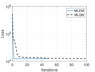
Refer to caption Refer to caption
Dataset A Dataset B
Refer to caption Refer to caption
Dataset C Dataset D
Figure 9: Evolution of 1:K(𝐀(i),𝐐(i))subscript:1𝐾superscript𝐀𝑖superscript𝐐𝑖\mathcal{L}_{1:K}({\mathbf{A}}^{(i)},{\mathbf{Q}}^{(i)}) along iterations using either MLEM or MLQN approach.

C.2 Robustness to initialization

DGLASSO algorithm amounts to minimizing a non-convex loss function. As such, its results might be sensitive to the initialization of the algorithm. To evaluate this aspect, we consider the computation of (𝐀^,𝐏^)^𝐀^𝐏(\widehat{{\mathbf{A}}},\widehat{{\mathbf{P}}}) given the observation of a single time series generated by the ground truth LG-SSM, when using 50 different initializations of DGLASSO algorithm. To do so, we use the same initialization strategy as discussed above, now with (a,p)𝑎𝑝(a,p) randomly selected as p𝒰([0,1])similar-to𝑝𝒰01p\sim\mathcal{U}([0,1]) and a𝒰([0,1])similar-to𝑎𝒰01a\sim\mathcal{U}([0,1]). Figure 10 displays the box plots for RMSE and F1 scores obtained for dataset A. One can notice that the box plots are very concentrated, showing a good robustness of the method to its initialization, with the wider spreading observed for the F1 score on 𝐀𝐀{\mathbf{A}}. Similar behavior was observed for the other three datasets.
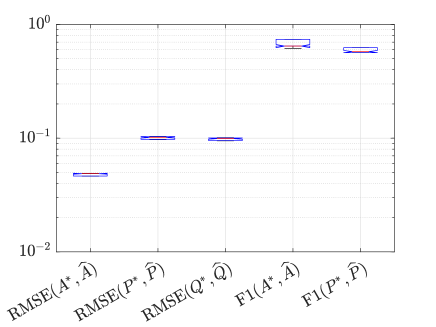
Refer to caption
Figure 10: Box plots for the RMSE and F1 scores for retrieving (𝐀,𝐏,𝐐)𝐀𝐏𝐐({\mathbf{A}},{\mathbf{P}},{\mathbf{Q}}) matrices, when running DGLASSO on one single LG-SSM time series using dataset A, and 50 random initializations (𝐀(0),𝐏(0))superscript𝐀0superscript𝐏0({\mathbf{A}}^{(0)},{\mathbf{P}}^{(0)}). Noticeably, low variability is observed for all metrics.

C.3 Influence of sparsity level

We evaluate here the performance of DGLASSO, as well as the benchmarks, when varying the sparsity level of the ground truth matrices. To do so, we perform slight changes in the dataset, to vary the sparsity pattern of the matrices (i.e., the edge structure of the graphs). First, we modify the ground truth matrix 𝐀superscript𝐀{\mathbf{A}}^{*} by keeping sA{27,15,10,5}subscript𝑠𝐴2715105s_{A}\in\{27,15,10,5\} entries of it, within the 272727 block diagonal ones, to be non-zero, the others being set to zero. We then rescaled the matrix to keep a spectral norm equals 0.990.990.99. Matrix 𝐐superscript𝐐{\mathbf{Q}}^{*} is taken from dataset A. The results are reported in Table 4.

As we can observe, the performance of MLEM, in terms of RMSE and F1 score, drop dramatically when the sparsity level on 𝐀𝐀{\mathbf{A}} increases. This is expected as this approach does not promote any sparsity prior on matrix 𝐀𝐀{\mathbf{A}}. The best AUC are either obtained by MLEM, DGLASSO or rGLASSO (for 𝐏𝐏{\mathbf{P}}), depending on the test cases. GLASSO/rGLASSO metrics slightly improve when 𝐀superscript𝐀{\mathbf{A}}^{*} gets sparser, which is expected, as their assumption of a zero transition matrix gets more realistic. Hereagain, DGLASSO outperforms the benchmarks in most cases.

Table 4: Results for sparsity levels sA{27,15,10,5}subscript𝑠𝐴2715105s_{A}\in\{27,15,10,5\} of 𝐀superscript𝐀{\mathbf{A}}^{*}, using (𝐏,𝐐)superscript𝐏superscript𝐐({\mathbf{P}}^{*},{\mathbf{Q}}^{*}) from dataset A. The first set of results, with sA=27subscript𝑠𝐴27s_{A}=27 identifies with the first row block of Tab. 1.
Estimation of 𝐀𝐀{\mathbf{A}} Estimation of 𝐏𝐏{\mathbf{P}} Estim. 𝐐𝐐{\mathbf{Q}} State distrib. Predictive distrib.
Method RMSE AUC F1 RMSE AUC F1 RMSE cNMSE(𝝁,𝝁^)superscript𝝁^𝝁(\bm{\mu}^{*},\widehat{\bm{\mu}}) cNMSE(𝝁s,𝝁^s)superscript𝝁ssuperscript^𝝁s(\bm{\mu}^{\text{s}*},\widehat{\bm{\mu}}^{\text{s}}) cNMSE(𝝂,𝝂^)superscript𝝂^𝝂({\bm{\nu}}^{*},\widehat{{\bm{\nu}}}) 1:K(𝐀^,𝐏^)subscript:1𝐾^𝐀^𝐏\mathcal{L}_{1:K}(\widehat{{\mathbf{A}}},\widehat{{\mathbf{P}}})
sA=27subscript𝑠𝐴27s_{A}=27 DGLASSO 0.060 5250.0605250.060\,525 0.842 550.842550.842\,55 0.640 570.640570.640\,57 0.081 9270.0819270.081\,927 0.778 010.778010.778\,01 0.698 120.698120.698\,12 0.082 6010.0826010.082\,601 6.393 5×𝟏𝟎𝟎𝟖6.3935E-086.393\,5\text{\times}{10}^{-08} 1.050 4×𝟏𝟎𝟎𝟕1.0504E-071.050\,4\text{\times}{10}^{-07} 2.983 7×𝟏𝟎𝟒2.9837E-42.983\,7\text{\times}{10}^{-4} 12 307.168 712307.168712\,307.168\,7
MLEM 0.076 0630.0760630.076\,063 0.816 930.816930.816\,93 0.50.50.5 0.105 280.105280.105\,28 0.857 390.857390.857\,39 0.50.50.5 0.101 520.101520.101\,52 1.094 7×10071.0947E-071.094\,7\text{\times}{10}^{-07} 1.802 5×10071.8025E-071.802\,5\text{\times}{10}^{-07} 4.842 5×1044.8425E-44.842\,5\text{\times}{10}^{-4} 12 341.204 512341.204512\,341.204\,5
GLASSO NA NA NA 0.818 380.818380.818\,38 0.803 940.803940.803\,94 0.496 160.496160.496\,16 1 073.510 41073.51041\,073.510\,4 4.485 3×10064.4853E-064.485\,3\text{\times}{10}^{-06} 7.180 4×10067.1804E-067.180\,4\text{\times}{10}^{-06} 111 28 459.293 528459.293528\,459.293\,5
rGLASSO NA NA NA 0.763 760.763760.763\,76 0.923 770.923770.923\,77 0.597 590.597590.597\,59 31.689 131.689131.689\,1 2.825 6×10062.8256E-062.825\,6\text{\times}{10}^{-06} 5.492 4×10065.4924E-065.492\,4\text{\times}{10}^{-06} 111 22 957.692 822957.692822\,957.692\,8
GRAPHEM 0.044 6310.0446310.044\,631 0.894 810.894810.894\,81 0.846 540.846540.846\,54 NA NA NA NA 4.364 2×10064.3642E-064.364\,2\text{\times}{10}^{-06} 6.944 3×10066.9443E-066.944\,3\text{\times}{10}^{-06} 2.98×1042.98E-42.98\text{\times}{10}^{-4} 29 035.029 629035.029629\,035.029\,6
sA=15subscript𝑠𝐴15s_{A}=15 DGLASSO 0.108 450.108450.108\,45 0.916 440.916440.916\,44 0.781 160.781160.781\,16 0.077 3960.0773960.077\,396 0.883 350.883350.883\,35 0.855 430.855430.855\,43 0.075 470.075470.075\,47 8.267 5×𝟏𝟎𝟎𝟕8.2675E-078.267\,5\text{\times}{10}^{-07} 1.157 4×𝟏𝟎𝟎𝟔1.1574E-061.157\,4\text{\times}{10}^{-06} 5.183×𝟏𝟎𝟑5.183E-35.183\text{\times}{10}^{-3} 11 801.220 211801.220211\,801.220\,2
MLEM 0.158 940.158940.158\,94 0.933 430.933430.933\,43 0.312 50.31250.312\,5 0.105 010.105010.105\,01 0.899 480.899480.899\,48 0.50.50.5 0.100 880.100880.100\,88 1.297 5×10061.2975E-061.297\,5\text{\times}{10}^{-06} 2.109 5×10062.1095E-062.109\,5\text{\times}{10}^{-06} 6.051 7×1036.0517E-36.051\,7\text{\times}{10}^{-3} 11 806.483 311806.483311\,806.483\,3
GLASSO NA NA NA 0.463 090.463090.463\,09 0.702 220.702220.702\,22 0.575 790.575790.575\,79 7.087 57.08757.087\,5 2.063 8×10052.0638E-052.063\,8\text{\times}{10}^{-05} 3.722 9×10053.7229E-053.722\,9\text{\times}{10}^{-05} 111 14 258.009 514258.009514\,258.009\,5
rGLASSO NA NA NA 0.424 590.424590.424\,59 0.722 550.722550.722\,55 0.597 720.597720.597\,72 4.562 44.56244.562\,4 1.378 9×10051.3789E-051.378\,9\text{\times}{10}^{-05} 2.768 4×10052.7684E-052.768\,4\text{\times}{10}^{-05} 111 14 432.765 314432.765314\,432.765\,3
GRAPHEM 0.126 80.12680.126\,8 0.927 660.927660.927\,66 0.720 610.720610.720\,61 NA NA NA NA 5.076 6×10055.0766E-055.076\,6\text{\times}{10}^{-05} 6.454 7×10056.4547E-056.454\,7\text{\times}{10}^{-05} 3.801 5×1033.8015E-33.801\,5\text{\times}{10}^{-3} 29 034.715 429034.715429\,034.715\,4
sA=10subscript𝑠𝐴10s_{A}=10 DGLASSO 0.089 2270.0892270.089\,227 0.981 440.981440.981\,44 0.938 490.938490.938\,49 0.083 7830.0837830.083\,783 0.767 860.767860.767\,86 0.685 620.685620.685\,62 0.084 4880.0844880.084\,488 9.385 6×𝟏𝟎𝟎𝟕9.3856E-079.385\,6\text{\times}{10}^{-07} 1.414 5×𝟏𝟎𝟎𝟔1.4145E-061.414\,5\text{\times}{10}^{-06} 9.747 5×𝟏𝟎𝟑9.7475E-39.747\,5\text{\times}{10}^{-3} 12 290.789 112290.789112\,290.789\,1
MLEM 0.167 310.167310.167\,31 0.999 940.999940.999\,94 0.219 780.219780.219\,78 0.105 360.105360.105\,36 0.899 590.899590.899\,59 0.50.50.5 0.101 030.101030.101\,03 2.383 1×10062.3831E-062.383\,1\text{\times}{10}^{-06} 3.917 9×10063.9179E-063.917\,9\text{\times}{10}^{-06} 2.591 7×1022.5917E-22.591\,7\text{\times}{10}^{-2} 11 819.738 911819.738911\,819.738\,9
GLASSO NA NA NA 0.364 810.364810.364\,81 0.666 670.666670.666\,67 0.50.50.5 0.468 890.468890.468\,89 3.025 8×10053.0258E-053.025\,8\text{\times}{10}^{-05} 5.958×10055.958E-055.958\text{\times}{10}^{-05} 111 13 173.462 113173.462113\,173.462\,1
rGLASSO NA NA NA 0.338 570.338570.338\,57 0.749 420.749420.749\,42 0.698 610.698610.698\,61 0.632 110.632110.632\,11 1.970 2×10051.9702E-051.970\,2\text{\times}{10}^{-05} 4.374 6×10054.3746E-054.374\,6\text{\times}{10}^{-05} 111 13 497.060 913497.060913\,497.060\,9
GRAPHEM 0.117 480.117480.117\,48 0.999 860.999860.999\,86 0.744 780.744780.744\,78 NA NA NA NA 8.955 6×10058.9556E-058.955\,6\text{\times}{10}^{-05} 1.124 4×1041.1244E-41.124\,4\text{\times}{10}^{-4} 1.225 5×1021.2255E-21.225\,5\text{\times}{10}^{-2} 29 034.726 829034.726829\,034.726\,8
sA=5subscript𝑠𝐴5s_{A}=5 DGLASSO 0.099 7340.0997340.099\,734 0.822 790.822790.822\,79 0.773 690.773690.773\,69 0.084 2390.0842390.084\,239 0.764 210.764210.764\,21 0.682 260.682260.682\,26 0.085 3780.0853780.085\,378 9.217 4×𝟏𝟎𝟎𝟕9.2174E-079.217\,4\text{\times}{10}^{-07} 1.205 5×𝟏𝟎𝟎𝟔1.2055E-061.205\,5\text{\times}{10}^{-06} 9.981 3×𝟏𝟎𝟑9.9813E-39.981\,3\text{\times}{10}^{-3} 12 268.667 112268.667112\,268.667\,1
MLEM 0.233 80.23380.233\,8 0.893 050.893050.893\,05 0.116 280.116280.116\,28 0.105 810.105810.105\,81 0.856 020.856020.856\,02 0.50.50.5 0.101 820.101820.101\,82 2.231 8×10062.2318E-062.231\,8\text{\times}{10}^{-06} 3.537 5×10063.5375E-063.537\,5\text{\times}{10}^{-06} 5.610 4×1025.6104E-25.610\,4\text{\times}{10}^{-2} 12 312.748 712312.748712\,312.748\,7
GLASSO NA NA NA 0.242 410.242410.242\,41 0.666 670.666670.666\,67 0.50.50.5 0.305 840.305840.305\,84 1.406 3×10051.4063E-051.406\,3\text{\times}{10}^{-05} 3.095 2×10053.0952E-053.095\,2\text{\times}{10}^{-05} 111 12 892.143 912892.143912\,892.143\,9
rGLASSO NA NA NA 0.261 810.261810.261\,81 0.703 540.703540.703\,54 0.566 270.566270.566\,27 0.451 220.451220.451\,22 1.195 3×10051.1953E-051.195\,3\text{\times}{10}^{-05} 2.884 2×10052.8842E-052.884\,2\text{\times}{10}^{-05} 111 12 834.736 712834.736712\,834.736\,7
GRAPHEM 0.127 230.127230.127\,23 0.930 530.930530.930\,53 0.573 280.573280.573\,28 NA NA NA NA 1.060 3×1041.0603E-41.060\,3\text{\times}{10}^{-4} 1.224 5×1041.2245E-41.224\,5\text{\times}{10}^{-4} 1.477×1021.477E-21.477\text{\times}{10}^{-2} 29 034.456 329034.456329\,034.456\,3

References

  • Alippi and Zambon (2023) C. Alippi and D. Zambon. Graph Kalman filters. Technical report, 2023. https://arxiv.org/pdf/2303.12021.pdf.
  • Andrieu et al. (2010) C. Andrieu, A. Doucet, and R. Holenstein. Particle Markov chain Monte Carlo methods. Journal of the Royal Statistical Society: Series B (Statistical Methodology), 72(3):269–342, 2010.
  • Attouch et al. (2010) H. Attouch, J. Bolte, P. Redont, and A. Soubeyran. Proximal alternating minimization and projection methods for nonconvex problems:an approach based on the kurdyka-lojasiewicz inequality. Mathematics of Operation Research, 35(2):438–457, 2010.
  • Attouch et al. (2013) H. Attouch, J. Bolte, and B. Svaiter. Convergence of descent methods for semi-algebraic and tame problems: proximal algorithms,forward–backward splitting. Mathematical Programming, 137(1):91–129, Feb. 2013.
  • Bach et al. (2012) F. Bach, R. Jenatton, J. Mairal, and G. Obozinski. Optimization with sparsity-inducing penalties. Foundations and Trends in Machine Learning, 4(1):1–106, Jan. 2012.
  • Bach and Jordan (2004) F. R. Bach and M. I. Jordan. Learning graphical models for stationary time series. IEEE Transactions on Signal Processing, 52(8):2189–2199, Aug. 2004. doi: 10.1109/TSP.2004.831032.
  • Barber and Cemgil (2010) D. Barber and A. T. Cemgil. Graphical models for time-series. IEEE Signal Processing Magazine, 27(6):18–28, Nov 2010. doi: 10.1109/MSP.2010.938028.
  • Bauschke and Combettes (2008) H. H. Bauschke and P. L. Combettes. A Dykstra-like algorithm for two monotone operators. Pacific Journal of Optimization, 4:383–391, 2008.
  • Bauschke and Combettes (2017) H. H. Bauschke and P. L. Combettes. Convex Analysis and Monotone Operator Theory in Hilbert Spaces. Springer, 2017. doi: 10.1007/978-3-319-48311-5.
  • Belilovsky et al. (2017) E. Belilovsky, K. Kastner, G. Varoquaux, and M. B. Blaschko. Learning to discover sparse graphical models. In Proceedings of the 34th International Conference on Machine Learning (ICML 2017), volume 70, pages 440–448, 2017.
  • Benfenati et al. (2018) A. Benfenati, E. Chouzenoux, L. Duval, J.-C. Pesquet, and A. Pirayre. A review on graph optimization and algorithmic frameworks. Technical report, 2018. https://hal.science/hal-01901499/document.
  • Benfenati et al. (2020) A. Benfenati, E. Chouzenoux, and J.-C. Pesquet. Proximal approaches for matrix optimization problems: Application to robust precision matrix estimation. Signal Processing, 169:107417, Apr. 2020.
  • Bolte et al. (2014) J. Bolte, S. Sabach, and M. Teboulle. Proximal alternating linearized minimization for nonconvex and nonsmooth problems. Mathematical Programming, 146(1):459–494, Aug. 2014.
  • Brendan and Tenenbaum (2010) L. Brendan and J. Tenenbaum. Discovering structure by learning sparse graphs. In Proceedings of the 32nd Annual Meeting of the Cognitive Science Society (CogSci 2010), pages 778–784, Portland, Oregon, USA, 11-14 Aug. 2010.
  • Briers et al. (2010) M. Briers, A. Doucet, and S. Maskell. Smooting algorithms for state-space models. Annals of the Institute of Statistical Mathematics, 62(61), 2010.
  • Bühlmann and Van De Geer (2011) P. Bühlmann and S. Van De Geer. Statistics for High-Dimensional Data: Methods, Theory and Applications. Springer Science & Business Media, 2011.
  • Cappe et al. (2005) O. Cappe, E. Moulines, and T. Ridden. Inference in Hidden Markov Models. Springer Series in Statistics. Springer New York, NY, 1st edition, 2005.
  • Chandrasekaran et al. (2012) V. Chandrasekaran, P. Parrilo, and A. Willsky. Latent variable graphical model selection via convex optimization. The Annals of Statistics, 40(4):1935–1967, 2012.
  • Chaux et al. (2007) C. Chaux, P. L. Combettes, J.-C. Pesquet, and V. R. Wajs. A variational formulation for frame-based inverse problems. Inverse Problems, 23(4):1495–1518, June 2007.
  • Chen et al. (2021) X. Chen, H. Wen, and Y. Li. Differentiable particle filters through conditional normalizing flow. In Proceedings of the IEEE 24th International Conference on Information Fusion (FUSION 2021), pages 1–6, 2021.
  • Cherni et al. (2020) A. Cherni, E. Chouzenoux, L. Duval, and J.-C. Pesquet. SPOQ lp-over-lq regularization for sparse signal recovery applied to mass spectrometry. IEEE Transactions on Signal Processing, 68:6070–6084, 2020.
  • Chopin et al. (2013) N. Chopin, P. E. Jacob, and O. Papaspiliopoulos. Smc2: an efficient algorithm for sequential analysis of state space models. Journal of the Royal Statistical Society Series B: Statistical Methodology, 75(3):397–426, 2013.
  • Chouzenoux and Elvira (2020) E. Chouzenoux and V. Elvira. GraphEM: EM algorithm for blind Kalman filtering under graphical sparsity constraints. In In Proceedings of the 45th IEEE International Conference on Acoustics, Speech, and Signal Processing (ICASSP 2020), pages 5840–5844, 4–8 May 2020.
  • Chouzenoux and Elvira (2023) E. Chouzenoux and V. Elvira. Graphit: Iterative reweighted l1 algorithm for sparse graph inference in state-space models. In Proceedings of the International Conference on Acoustics, Speech, and Signal Processing (ICASSP 2023), Rhodes Island, Greece, 4-10 June 2023.
  • Chouzenoux et al. (2014) E. Chouzenoux, J.-C. Pesquet, and A. Repetti. Variable metric forward-backward algorithm for minimizing the sum of a differentiable function and a convex function. Journal of Optimization Theory and Applications, 162(1):107–132, 2014.
  • Chouzenoux et al. (2016) E. Chouzenoux, J.-C. Pesquet, and A. Repetti. A block coordinate variable metric forward-backward algorithm. Journal of Global Optimization, 66(3):457–485, 2016.
  • Chouzenoux et al. (2019) E. Chouzenoux, T. T.-K. Lau, and J.-C. Pesquet. Optimal multivariate Gaussian fitting with applications to PSF modeling in two-photon microscopy imaging. Journal of Mathematical Imaging and Vision, 61(7):1037–1050, 2019.
  • Combettes and Pesquet (2011) P. L. Combettes and J.-C. Pesquet. Proximal splitting methods in signal processing. In Fixed-point algorithms for inverse problems in science and engineering, pages 185–212. Springer, 2011.
  • Corenflos et al. (2021) A. Corenflos, J. Thornton, G. Deligiannidis, and A. Doucet. Differentiable particle filtering via entropy-regularized optimal transport. In Proceedings of the 38th International Conference on Machine Learning (ICML 2021), page 2100–2111, Jul 2021.
  • Cox and Elvira (2022) B. Cox and V. Elvira. Parameter estimation in sparse linear-Gaussian state-space models via reversible jump Markov Chain Monte Carlo. In Proceedings of the 30th European Signal Processing Conference (EUSIPCO 2022), pages 797–801, Belgrade, Serbia, 29 Aug.-2 Sep. 2022.
  • Cox and Elvira (2023) B. Cox and V. Elvira. Sparse Bayesian estimation of parameters in linear-Gaussian state-space models. IEEE Transactions on Signal Processing (to appear in), 2023.
  • Crisan and Miguez (2018) D. Crisan and J. Miguez. Nested particle filters for online parameter estimation in discrete-time state-space markov models. 2018.
  • Dempster et al. (1977) A. P. Dempster, N. M. Laird, and D. B. Rubin. Maximum likelihood from incomplete data via the em algorithm. Journal of the Royal Statistical Society. Series B (Methodological), 39(1):1–38, 1977.
  • Djuric et al. (2003) P. M. Djuric, J. H. Kotecha, J. Zhang, Y. Huang, T. Ghirmai, M. F. Bugallo, and J. Miguez. Particle filtering. IEEE signal processing magazine, 20(5):19–38, 2003.
  • Doucet et al. (2009) A. Doucet, A. M. Johansen, et al. A tutorial on particle filtering and smoothing: Fifteen years later. Handbook of nonlinear filtering, 12(656-704):3, 2009.
  • Eichler (2012) M. Eichler. Graphical modelling of multivariate time series. Probability Theory and Related Fields, 153(1):233–268, Jun. 2012. ISSN 1432-2064. doi: 10.1007/s00440-011-0345-8. URL https://doi.org/10.1007/s00440-011-0345-8.
  • Elvira and Chouzenoux (2022) V. Elvira and E. Chouzenoux. Graphical inference in linear-Gaussian state-space models. IEEE Transactions on Signal Processing, 70:4757–4771, 2022.
  • Frenkel and Feder (1999) L. Frenkel and M. Feder. Recursive expectation-maximization (EM) algorithms for time-varying parameters with applications to multiple target tracking. IEEE Transactions on Signal Processing, 47(2):306–320, 1999.
  • Friedman et al. (2008) J. Friedman, T. Hastie, and R. Tibshirani. Sparse inverse covariance estimation with the graphical LASSO. Biostatistics, 9(3):432–441, jul 2008.
  • Gao et al. (2015) R. Gao, F. Tronarp, and S. Sarkka. Iterated extended Kalman smoother-based variable splitting for l1-regularized state estimation. IEEE Transactions on Signal Processing, 67(19):5078–5092, 2015.
  • Giannakis et al. (2018) G. Giannakis, Y. Shen, and G. Karanikolas. Topology identification and learning over graphs: Accounting for nonlinearities and dynamics. Proceedings of the IEEE, 106(5):787–807, May 2018.
  • Granger (1969) C. W. Granger. Investigating causal relations by econometric models and cross-spectral methods. Econometrica: Journal of the Econometric Society, pages 424–438, 1969.
  • Green and Hastie (2009) P. J. Green and D. I. Hastie. Reversible jump MCMC. Genetics, 155(3):1391–1403, 2009.
  • Gupta and Mehra (1974) N. Gupta and R. Mehra. Computational aspects of maximum likelihood estimation and reduction in sensitivity function calculations. IEEE Transactions on Automatic Control, 19(6):774–783, 1974.
  • Hamilton (1994) J. D. Hamilton. State-space models. Handbook of Econometrics, 4:3039–3080, 1994.
  • Hamilton (2020) J. D. Hamilton. Time series analysis. Princeton university press, 2020.
  • Hien et al. (2020) T. Hien, N. Gillis, and P. Patrinos. Inertial block proximal method for non-convex nonsmooth optimization. In Proceedings of the Thirty-seventh International Conference on Machine Learning (ICML 2020), 2020.
  • Hippert-Ferrer et al. (2022) A. Hippert-Ferrer, F. Bouchard, A. Mian, T. Vayer, and A. Breloy. Learning graphical factor models with Riemannian optimization. Technical report, 2022. https://arxiv.org/abs/2210.11950.
  • Hong et al. (2016) M. Hong, M. Razaviyayn, Z.-Q. Luo, and J. S. Pang. A unified algorithmic framework for block-structured optimization involving big data: With applications in machine learning and signal processing. IEEE Signal Process. Mag., 33(1):57–77, Jan. 2016.
  • Hunter and Lange (2004) D. R. Hunter and K. Lange. A tutorial on MM algorithms. Amer. Stat., 58(1):30–37, Feb. 2004.
  • Ioannidis et al. (2018) V. Ioannidis, D. Romero, and G. Giannakis. Inference of spatio-temporal functions over graphs via multikernel kriged Kalman filtering. IEEE Transactions on Signal Processing, 66(12):3228–3239, 2018.
  • Ioannidis et al. (2019) V. Ioannidis, Y. Shen, and G. Giannakis. Semi-blind inference of topologies and dynamical processes over dynamic graphs. IEEE Transactions on Signal Processing, 67(9):2263–2274, May 2019.
  • Jacobson and Fessler (2007) M. Jacobson and J. Fessler. An expanded theoretical treatment of iteration-dependent majorize-minimize algorithms. IEEE Transactions on Image Processing, 16(10):2411–2422, 2007.
  • Kalman (1960) R. E. Kalman. A new approach to linear filtering and prediction problems. Journal of Basic Engineering, 82:35–45, 1960.
  • Kantas et al. (2015) N. Kantas, A. Doucet, S. S. Singh, J. Maciejowski, and N. Chopin. On particle methods for parameter estimation in state-space models. Technical report, 2015. https://arxiv.org/abs/1412.8695.
  • Kim and Nelson (1999) C.-J. Kim and C. R. Nelson. State-space models with regime switching: classical and Gibbs-sampling approaches with applications. MIT Press Books, 1st edition, 1999.
  • Komodakis and Pesquet (2015) N. Komodakis and J.-C. Pesquet. Playing with duality: An overview of recent primal-dual approaches for solving large-scale optimization problems. IEEE Signal Processing Magazine, 32(6):31–54, 2015.
  • Kumar et al. (2020) S. Kumar, J. Ying, J. V. de Miranda Cardoso, and D. P. Palomar. A unified framework for structured graph learning via spectral constraints. Journal of Machine Learning Research, 21(22):1–60, 2020.
  • Lojasiewicz (1963) S. Lojasiewicz. Unepropriété topologique des sous-ensembles analytiques réels. Editions du Centre National de la Recherche Scientifique, pages 87–89, 1963.
  • Luengo et al. (2019) D. Luengo, G. Rios-Munoz, V. Elvira, C. Sanchez, and A. Artes-Rodriguez. Hierarchical algorithms for causality retrieval in atrial fibrillation intracavitary electrograms. IEEE Journal of Biomedical and Health Informatics, 12(1):143–155, Jan. 2019.
  • Maathuis et al. (2019) M. Maathuis, M. Drton, S. Lauritzen, and M. Wainwright. Handbook of Graphical Models. CRC Press, Boca Raton, FL, 2019.
  • Meinshausen and Bühlmann (2006) N. Meinshausen and P. Bühlmann. High-dimensional graphs and variable selection with the lasso. The Annals of Statistics, pages 1436–1462, 2006.
  • Moré and Toraldo (1989) J. Moré and G. Toraldo. Algorithms for bound constrained quadratic programming problems. Numerical Mathematics, 55:377–400, 1989.
  • Naesseth et al. (2019) C. A. Naesseth, F. Lindsten, T. B. Schön, et al. Elements of sequential monte carlo. Foundations and Trends® in Machine Learning, 12(3):307–392, 2019.
  • Nagakura (2021) D. Nagakura. Computing exact score vectors for linear Gaussian state space models. Communications in Statistics - Simulation and Computation, 50(8):2313–2326, 2021.
  • Olsson et al. (2007) R. Olsson, K. Petersen, and T. Lehn-Schioler. State-space models: from the EM algorithm to a gradient approach. Neural Computation, 19(4):1097–1111, 2007.
  • Pérez-Vieites and Míguez (2021) S. Pérez-Vieites and J. Míguez. Nested gaussian filters for recursive bayesian inference and nonlinear tracking in state space models. Signal Processing, 189:108295, 2021.
  • Runge et al. (2020) J. Runge, X.-A. Tibau, M. Bruhns, J. Muñoz-Marí, and G. Camps-Valls. The causality for climate competition. In Proceedings of the NeurIPS 2019 Competition and Demonstration Track, volume 123, pages 110–120, 2020.
  • Sagi et al. (2023) G. Sagi, N. Shlezinger, and T. Routtenberg. Extended Kalman filter for graph signals in nonlinear dynamic systems. In Proceedings of the International Conference on Acoustics, Speech, and Signal Processing (ICASSP 2023), Rhodes Island, Greece, 4-10 June 2023.
  • Sarkka (2013) S. Sarkka. Bayesian Filtering and Smoothing. 3 edition, 2013.
  • Segal and Weinstein (1988) M. Segal and E. Weinstein. A new method for evaluating the log-likelihood gradient (score) of linear dynamic systems. IEEE Transactions on Automatic Control, 33(8):763–766, 1988. doi: 10.1109/9.1295.
  • Segal and Weinstein (1989) M. Segal and E. Weinstein. A new method for evaluating the log-likelihood gradient, the hessian, and the fisher information matrix for linear dynamic systems. IEEE Transactions on Information Theory, 35(3):682–687, 1989. doi: 10.1109/18.30995.
  • Sharma et al. (2020) S. Sharma, A. Majumdar, V. Elvira, and E. Chouzenoux. Blind Kalman filtering for short-term load forecasting. IEEE Transactions on Power Systems, 35(6):4916–4919, Nov. 2020.
  • Sharma et al. (2021) S. Sharma, V. Elvira, E. Chouzenoux, and A. Majumdar. Recurrent dictionary learning for state-space models with an application in stock forecasting. Neurocomputing, 450:1–13, Aug. 2021.
  • Shojaie and Michailidis (2010) A. Shojaie and G. Michailidis. Discovering graphical granger causality using the truncating lasso penalty. Bioinformatics, 26(18):i517–i523, 2010.
  • Shumway and Stoffer (1982) R. H. Shumway and D. S. Stoffer. An approach to time series smoothing and forecasting using the EM algorithm. Journal of Time Series Analysis, 3(4):253–264, 1982.
  • Sun et al. (2016) Y. Sun, P. Babu, and D. P. Palomar. Majorization-minimization algorithms in signal processing, communications, and machine learning. IEEE Transactions on Signal Processing, 65(3):794 – 816, 2016.
  • Tibshirani (1996) R. Tibshirani. Regression shrinkage and selection via the lasso. Journal of the Royal Statistical Society. Series B (Methodological), 58(1):267–288, 1996.
  • Tien et al. (2020) L. T. K. Tien, D. N. Phan, and N. Gillis. An inertial block majorization minimization framework for nonsmooth nonconvex optimization. Technical report, 2020. https://arxiv.org/abs/2010.12133.
  • Uhler (2017) C. Uhler. Gaussian graphical models: An algebraic and geometric perspective. Technical report, 2017. https://arxiv.org/abs/1707.04345.
  • Wu (1983) C. F. J. Wu. On the convergence properties of the EM algorithm. The Annals of Statistics, 11(1):95–103, 1983.
  • Ying et al. (2020) J. Ying, J. V. d. M. Cardoso, and D. P. Palomar. Does the 1subscript1\ell_{1}-norm learn a sparse graph under Laplacian constrained graphical models? Technical report, 2020. https://arxiv.org/abs/2006.14925.