Value of Information in Games with Multiple Strategic Information Providersthanks: Research of the authors was supported in part by the ARO MURI Grant AG285 and in part by ARL-DCIST Grant AK868.

Raj Kiriti Velicheti   Melih Bastopcu   Tamer Başar
Coordinated Science Laboratory
University of Illinois Urbana-Champaign
Urbana IL 61801
(rkv4,bastopcu,basar1)@illinois.edu
Abstract

In the classical communication setting multiple senders having access to the same source of information and transmitting it over channel(s) to a receiver in general leads to a decrease in estimation error at the receiver as compared with the single sender case. However, if the objectives of the information providers are different from that of the estimator, this might result in interesting strategic interactions and outcomes. In this work, we consider a hierarchical signaling game between multiple senders (information designers) and a single receiver (decision maker) each having their own, possibly misaligned, objectives. The senders lead the game by committing to individual information disclosure policies simultaneously, within the framework of a non-cooperative Nash game among themselves. This is followed by the receiver’s action decision. With Gaussian information structure and quadratic objectives (which depend on underlying state and receiver’s action) for all the players, we show that in general the equilibrium is not unique. We hence identify a set of equilibria and further show that linear noiseless policies can achieve a minimal element of this set. Additionally, we show that competition among the senders is beneficial to the receiver, as compared with cooperation among the senders. Further, we extend our analysis to a dynamic signaling game of finite horizon with Markovian information evolution. We show that linear memoryless policies can achieve equilibrium in this dynamic game. We also consider an extension to a game with multiple receivers having coupled objectives. We provide algorithms to compute the equilibrium strategies in all these cases. Finally, via extensive simulations, we analyze the effects of multiple senders in varying degrees of alignment among their objectives.

I Introduction

With increasing ease of communication and emergence of remote estimation, questions about the incentives of the data sources take the center stage. Consider, for example, the community notes feature rolled out recently by Twitter to combat misinformation. This feature lets volunteered users to post a note on a Tweet that might possibly be incorrect. However, since this may lead to strategic reporting, Twitter further aggregates data from a group of volunteers with diverse views. This brings us to the following two questions: How diverse should the views be? Is there a systematic way to understand the amount of information revealed given a prior on possible personal biases that people can have? As another example, consider a robot learning to perform a task based on human demonstrations. In order to perform the task efficiently a large number of human demonstrations need to be collected but since humans might have their own biases, this causes a possible mismatch in objectives[1]. Learning the underlying task amidst these mismatched (possibly strategic) objectives is still a problem of active interest[2]. Such an estimation with strategic sources occurs in multiple situations including estimation from strategic sensors in cyber-physical systems, Federated Learning, and information theory [3, 4, 5]. We aim to model these interactions as a communication game and analyze the resulting outcome.

A model of strategic communication was introduced in the seminal work [6] which considers a game between a sender and a receiver with simultaneous strategy commitment. Different from the traditional communication setting, their work considers a sender and a receiver with mismatched objectives and noise-free channels, which makes the problem a communication game. Under few regularity assumptions, they have shown that all Nash Equilibria are quantization based mappings. Following [6], several extensions to the model have been considered in the literature such as multiple senders[7, 8], adding of a strategic mediation channel[9], considering dynamic information disclosure[10], and multidimensional settings[11], all under Nash equilibrium.

An alternate line of work pioneered in [12, 13] (termed as Bayesian Persuasion), however, considers instead a hierarchical signaling game where the receiver responds to a strategy committed by the sender. This commitment power adds benefit to the sender, and hence can be used to characterize the optimal utility that a sender can derive in such a communication game. The key idea to solve for the optimal sender strategy in such a game is to pose an equivalent optimization problem in the space of posteriors using the splitting lemma [14]. Due to the natural hierarchical structure occurring in many scenarios, (such as the ones described earlier), the last decade has seen a surge of interest in this model from various disciplines including control theory[15, 11, 16], machine learning [17], information theory [18], and mechanism design[19]. A follow-up work [20] identifies that the optimal sender strategy can be computed by solving a linear program. Extensions to the dynamic case with discrete states evolving as a Markov chain are studied in [21, 22]. [23] provides a more detailed review regarding recent works along this line. Additionally, outside the communication context, games with mismatched objectives between multiple principals (players who are similar to senders in this work) and a social optimizer are considered broadly under the name of common agent games in [24, 25].

In spirit, our work adds on to the growing literature of multi-sender hierarchical communication games. References [26, 27] solve for Nash equilibrium (NE) among senders, assuming access to arbitrarily correlated signaling policies, by utilizing concavification. They show that there can be more than one equilibrium with full revelation by all senders always being an equilibrium. Such intuitive results also extend to our setting although proving them requires different mathematical tools which we will formalize in the following sections. Studies in [28, 29] consider a slightly different game where senders can commit sequentially and prove the uniqueness of equilibrium in such a game. On the other hand, works [30, 31, 32] analyze a game consisting of multiple receivers and investigate the effects of public and private signaling but confine attention to a single sender. All these works mentioned above consider finite state and action spaces where state is a one-dimensional variable.

In contrast, in this work we consider a more general infinite multidimensional state and action spaces while restricting our attention to a Gaussian prior and quadratic utilities. Multidimensional signaling games require a significantly different set of tools than those described previously. In one of the initial works in this direction, [33] utilizes semi-definite programming (SDP) to solve for a lower bound on sender’s cost111In line with the control literature, most of the works discussed here consider the scenario where each player wants to minimize their individual cost function rather than maximize their own utility function. and prove that for Gaussian information structures, linear policies can be used to achieve this lower bound. Reference [34] extends this by considering a dynamic sender receiver game and shows that equilibrium posteriors follow a recursive structure which can still be achieved by using linear policies. [35] shows that noisy linear policies are sufficient to identify an SDP which is equivalent to sender’s optimization problem. Reference [36] goes beyond Gaussian distribution and utilizes techniques from co-positive programming to identify lower bounds for arbitrary prior distributions when players have quadratic objectives. Finally, [33] mentions a game with multiple senders as an extension to their earlier work, and presents a necessary condition for existence of a partially revealing equilibrium for the underlying game. However, [33] does not characterize equilibrium posteriors nor do they specify Nash equilibrium strategies for the senders. Although [15] considers the multi-sender communication game, it restricts attention to symmetric sender objectives while allowing for private realization of state for each sender and solving for a herding equilibrium.

Coming to the specifics of this paper, our contributions are multi-fold. Firstly, we pose a strategic communication game between multiple senders and a single receiver. We then solve for a hierarchical equilibrium where all senders commit to an information disclosure strategy222In this work, we use the terms strategy and policy interchangeably. simultaneously (and thus, play a Nash game among themselves) followed by the receiver taking a decision (and as a result, play a Stackelberg game between senders and the receiver)[37]. Due to the presence of multiple senders, each sender faces an equilibrium computation problem which can be significantly different from the optimization problem in a single sender game discussed in [33, 34].In particular, each sender needs to compute a strategy accounting for the presence of other senders with possibly misaligned utilities. Further, as will be illustrated in the following sections, the game under consideration is a general sum game but is not convex in each players action. To ease computation of the equilibrium, we pose the problem in space of posterior covariance, propose a notion of stable posterior and design an algorithm to identify such posteriors. We show that the equilibrium might not be unique and identify necessary conditions that equilibrium policies should satisfy. Additionally, we propose an equilibrium refinement, termed as partially informative equilibrium, to identify equilibria which are robust against more informative deviation by all the senders. Although noiseless signaling policies restrict the space of possible posteriors[33], we show that these equilibria can be achieved by linear noiseless signaling policies. For ease of exposition, we start by considering a game with two senders and a single receiver and then extend it to a game with more than two senders. Next, we formulate a dynamic game and extend the result of [34] to the multiple-sender setting. We show that greedy equilibrium computation for a single stage game results in posteriors that are stable for the dynamic game, and thus we identify a recursive structure for equilibrium posteriors. Further, similar to the single-stage case, we also show that these equilibrium posteriors can be achieved by linear noiseless signaling policies. We also provide extension to a game with multiple receivers with possibly coupled objectives. Finally, we provide extensive numerical results to demonstrate the effect of competition in information revelation. A key takeaway from our work, apart from the technical tools developed, is that in line with [26], even in multidimensional infinite state spaces with quadratic cost333In this work we use the terms objective and cost interchangeably. functions, competition among multiple senders is beneficial to the receiver. However, unlike in [26], we do not require arbitrary correlation between senders’ signaling policies, and thus overcome limitations of the work in [26].

The paper is organized as follows: In Section II, we introduce our system model with a single-stage and formulate the strategic information disclosure problem for an m𝑚m-sender and a single receiver game. In Section III, we first consider a sub-class with 2 senders and identify the equilibrium policies and prove the optimality of linear policies. Then, we extend this result to a more general case with m>2𝑚2m>2 senders. In Section IV, we formulate the multi-stage dynamic strategic information disclosure problem with multiple senders. Here, we show that applying the same solution technique developed for the single-stage problem greedily to the multi-stage game achieves the equilibrium, which can also be obtained by using linear signaling strategies. In Section V, we extend our results to a game with multiple receivers. In Section VI, we provide extensive numerical results to understand the effect of multiple senders and the achieved equilibrium policies in various scenarios. Section VII provides insights on the commitment structure assumed in this work and discusses other possible equilibrium definitions for multi-sender games. Finally, we conclude the paper with some major highlights of our work and potential future directions in Section VIII.

Notations

We denote by [m]delimited-[]𝑚[m] the set {1,,m}1𝑚\{1,\dots,m\}. (0,Σ)0Σ\mathbb{N}(0,\Sigma) denotes a Gaussian distribution with mean 0 and co-variance ΣΣ\Sigma where ΣΣ\Sigma is a positive semi-definite (psd) matrix. For a psd matrix S𝑆S, we use S12superscript𝑆12S^{\frac{1}{2}} to denote its unique psd square root. We use 𝒩(.)\mathcal{N}(.) to denote the null set of a matrix. 𝒩¯¯𝒩\bar{\mathcal{N}} denotes a set of possible ordering. Tr(.)Tr(.) denotes the trace of a matrix. We denote vectors with bold lower symbols. For a given matrix A𝐴A and a vector 𝒚𝒚\bm{y}, Asuperscript𝐴topA^{\top} and 𝒚superscript𝒚top\bm{y}^{\top} denote the transposes of that matrix and the vector, respectively. We use Bsuperscript𝐵B^{\dagger} to denote the pseudo-inverse of matrix B𝐵B. The identity and zero matrices are denoted by I𝐼I and O𝑂O, respectively. For two symmetric matrices A𝐴A and B𝐵B, ABsucceeds𝐴𝐵A\succ B (ABsucceeds-or-equals𝐴𝐵A\succeq B) means that AB𝐴𝐵A-B is a positive (semi-)definite matrix. For a set 𝑿𝑿\bm{X}, we use (𝑿)𝑿\mathcal{B}(\bm{X}) to denote the Borel set of 𝑿𝑿\bm{X}.

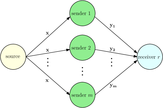
Refer to caption

Figure 1: The strategic communication system consisting of m𝑚m senders denoted by i=1,,m𝑖1𝑚i=1,\dots,m and a receiver r𝑟r. Each sender i𝑖i observes the state of the world 𝒙𝒙\bm{x} and designs its signaling policy so as to minimize its cost Jisubscript𝐽𝑖J_{i} while the receiver estimates the state of the world based on the signals that it receives to minimize its cost Jrsubscript𝐽𝑟J_{r}.

II System Model and Problem Formulation

Consider a non-cooperative game among a group of m+1𝑚1m+1 players, comprised of m𝑚m senders denoted by i=1,,m𝑖1𝑚i=1,\dots,m, and a receiver denoted by r𝑟r. The senders have access to a random state variable 𝒙𝑿p𝒙𝑿superscript𝑝\bm{x}\in\bm{X}\subseteq\mathbb{R}^{p}, which is sampled from a zero-mean Gaussian distribution with positive-definite covariance ΣxsubscriptΣ𝑥\Sigma_{x}, i.e., 𝒙(0,Σx)similar-to𝒙0subscriptΣ𝑥\bm{x}\sim\mathbb{N}(0,\Sigma_{x}) with ΣxOsucceedssubscriptΣ𝑥𝑂\Sigma_{x}\succ O. After observing the state realization 𝒙𝒙\bm{x}, the senders send signals {𝒚i}i[m]subscriptsubscript𝒚𝑖𝑖delimited-[]𝑚\{\bm{y}_{i}\}_{i\in[m]} to the receiver. After observing these signals, the receiver forms an estimate of 𝒙𝒙\bm{x} and takes an action 𝒖𝒖\bm{u}. Thus, let the action of sender i𝑖i be 𝒚i𝒀isubscript𝒚𝑖subscript𝒀𝑖\bm{y}_{i}\in\bm{Y}_{i} and that of the receiver be 𝒖𝑼𝒖𝑼\bm{u}\in\bm{U}, where 𝒀ipsubscript𝒀𝑖superscript𝑝\bm{Y}_{i}\subseteq\mathbb{R}^{p} and 𝐔t𝐔superscript𝑡\mathbf{U}\subseteq\mathbb{R}^{t} are the action spaces of sender i𝑖i and the receiver, respectively.

All players have their own individual loss functions Li(𝒙;𝒖)subscript𝐿𝑖𝒙𝒖L_{i}(\bm{x};\bm{u}) for i=1,,m,r𝑖1𝑚𝑟i=1,\ldots,m,r, mapping from 𝑿×𝑼𝑿𝑼\bm{X}\times\bm{U}\rightarrow\mathbb{R}. Let Ii(𝑿×𝒀1×𝒀m)subscript𝐼𝑖𝑿subscript𝒀1subscript𝒀𝑚I_{i}\subseteq\mathcal{B}(\bm{X}\times\bm{Y}_{1}\times\ldots\bm{Y}_{m}) denote the information structure of player i=1,,m,r𝑖1𝑚𝑟i=1,\ldots,m,r. Formally, we have Ii={𝒙}subscript𝐼𝑖𝒙I_{i}=\{\bm{x}\} for all the senders i[m]𝑖delimited-[]𝑚i\in[m] and Ir={𝒚1,,𝒚m}subscript𝐼𝑟subscript𝒚1subscript𝒚𝑚I_{r}=\{\bm{y}_{1},\ldots,\bm{y}_{m}\} as shown in Fig. 1. We specifically consider quadratic loss functions which are of the form:

Li(𝒙;𝒖)=Qi𝒙+Ri𝒖2,i=1,,m,r.formulae-sequencesubscript𝐿𝑖𝒙𝒖superscriptnormsubscript𝑄𝑖𝒙subscript𝑅𝑖𝒖2𝑖1𝑚𝑟\displaystyle L_{i}(\bm{x};\bm{u})=\|Q_{i}\bm{x}+R_{i}\bm{u}\|^{2},\quad i=1,\ldots,m,r. (1)

Let the strategy of sender i𝑖i be ηi:Ii𝒀i:subscript𝜂𝑖subscript𝐼𝑖subscript𝒀𝑖\eta_{i}:I_{i}\rightarrow\bm{Y}_{i} such that 𝒚i=ηi(𝒙)subscript𝒚𝑖subscript𝜂𝑖𝒙\bm{y}_{i}=\eta_{i}(\bm{x}) is transmitted to the receiver. We denote by ΩΩ\Omega the policy space of each sender (i.e., ηiΩsubscript𝜂𝑖Ω\eta_{i}\in\Omega for i[m]𝑖delimited-[]𝑚i\in[m]) which we consider to be the space of all Borel-measurable functions from psuperscript𝑝\mathbb{R}^{p} to psuperscript𝑝\mathbb{R}^{p}.444We note that this is the most general case that provides maximum flexibility to the sender. As to be shown through simulations in Section VI a message space ssuperscript𝑠\mathbb{R}^{s} with s<p𝑠𝑝s<p suffices in specific instances. Let the strategy of the receiver be γ:Ir𝑼:𝛾subscript𝐼𝑟𝑼\gamma:I_{r}\rightarrow\bm{U} such that the receiver selects an action 𝐮=γ({𝒚i}i[m])𝐮𝛾subscriptsubscript𝒚𝑖𝑖delimited-[]𝑚\mathbf{u}=\gamma(\{\bm{y}_{i}\}_{i\in[m]}) based on the policy γΓ𝛾Γ\gamma\in\Gamma where ΓΓ\Gamma is a set of all Borel measurable functions from mpsuperscript𝑚𝑝\mathbb{R}^{mp} to tsuperscript𝑡\mathbb{R}^{t}. Finally, the expected cost function of each player i=1,,m,r𝑖1𝑚𝑟i=1,\ldots,m,r is given by

Ji(η1,,ηm;γ)=𝔼[Li(𝒙;𝒖=γ(Ir))],subscript𝐽𝑖subscript𝜂1subscript𝜂𝑚𝛾𝔼delimited-[]subscript𝐿𝑖𝒙𝒖𝛾subscript𝐼𝑟\displaystyle J_{i}(\eta_{1},\ldots,\eta_{m};\gamma)=\mathbb{E}[L_{i}(\bm{x};\bm{u}=\gamma(I_{r}))], (2)

where the dependence on ηisubscript𝜂𝑖\eta_{i} appears through the information structure of the receiver, Irsubscript𝐼𝑟I_{r}.

We consider a hierarchical commitment structure where the senders announce, and thus commit to their policies followed by the receiver’s reaction optimizing its expected cost. This structure leads to a Nash game played between the senders, followed by a Stackelberg game between the senders and the receiver[37]. Due to this commitment structure, the receiver’s strategy γ𝛾\gamma can depend on senders’ signaling policies, i.e., γ({𝒚i}i[m])=γ({ηi}i[m])({𝒚i}i[m])𝛾subscriptsubscript𝒚𝑖𝑖delimited-[]𝑚𝛾subscriptsubscript𝜂𝑖𝑖delimited-[]𝑚subscriptsubscript𝒚𝑖𝑖delimited-[]𝑚\gamma(\{\bm{y}_{i}\}_{i\in[m]})=\gamma(\{\eta_{i}\}_{i\in[m]})(\{\bm{y}_{i}\}_{i\in[m]}). Let Γ({ηi}i[m])superscriptΓsubscriptsubscript𝜂𝑖𝑖delimited-[]𝑚\Gamma^{*}(\{\eta_{i}\}_{i\in[m]}) denote receiver r𝑟r’s best response set for given tuple of senders’ policies ({ηi}i[m])subscriptsubscript𝜂𝑖𝑖delimited-[]𝑚(\{\eta_{i}\}_{i\in[m]}). This is a subset of ΓΓ\Gamma and is given by the following expression where we assume that a minimum exists (which turns out to be the case as to be shown later):

Γ({ηi}i[m])=argminγΓJr({ηi}i[m],γ({ηi}i[m])).superscriptΓsubscriptsubscript𝜂𝑖𝑖delimited-[]𝑚subscript𝛾Γsubscript𝐽𝑟subscriptsubscript𝜂𝑖𝑖delimited-[]𝑚𝛾subscriptsubscript𝜂𝑖𝑖delimited-[]𝑚\displaystyle\Gamma^{*}(\{\eta_{i}\}_{i\in[m]})=\operatorname*{\arg\!\min}_{\gamma\in\Gamma}J_{r}(\{\eta_{i}\}_{i\in[m]},\gamma(\{\eta_{i}\}_{i\in[m]})).

Under certain assumptions such as the convexity of the receiver’s utility, which is true in our setting due to the quadratic cost structure as given by (1), the receiver’s best response set ΓsuperscriptΓ\Gamma^{*} forms an equivalence class, and hence results in the same random variable 𝒖𝒖\bm{u} for any γΓsuperscript𝛾superscriptΓ\gamma^{*}\in\Gamma^{*} almost surely. Therefore, the set of signaling rules ({ηi}i[m],γ)subscriptsubscriptsuperscript𝜂𝑖𝑖delimited-[]𝑚superscript𝛾(\{\eta^{*}_{i}\}_{i\in[m]},\gamma^{*}) are said to achieve equilibrium if

Ji(ηi,{ηi},γ(ηi,{ηi}))Ji(ηi,{ηi},γ(ηi,{ηi})),ηiΩ,i[m],γ({ηi}i[m])=argminγΓJr({ηi}i[m],γ({ηi}i[m]),\displaystyle\begin{split}J_{i}(\eta_{i}^{*},\{\eta_{-i}^{*}\},\gamma^{*}(\eta_{i}^{*},\{\eta_{-i}^{*}\}))&\leq J_{i}(\eta_{i},\{\eta_{-i}^{*}\},\gamma^{*}(\eta_{i},\{\eta_{-i}^{*}\})),\quad\forall\eta_{i}\in\Omega,\forall i\in[m],\\ \gamma^{*}(\{\eta_{i}\}_{i\in[m]})&=\operatorname*{\arg\!\min}_{\gamma\in\Gamma}J_{r}(\{\eta_{i}\}_{i\in[m]},\gamma(\{\eta_{i}\}_{i\in[m]}),\end{split} (3)

where ηisuperscriptsubscript𝜂𝑖\eta_{-i}^{*} denotes the equilibrium strategies of all senders other than sender i𝑖i, and we assumed that the best response set of the receiver, ΓsuperscriptΓ\Gamma^{*}, forms an equivalence class, and thus leads to a unique 𝒖𝒖\bm{u} almost surely.

Note that in the equilibrium formulation provided in (3), all senders select their strategies independent of the signal realizations. Thus each sender is assumed to minimize its expected cost. In the following section we analyze equilibrium strategies for all players considering quadratic costs.

III Multi Sender Strategic Information Disclosure

In this section, we first start by considering a three-player communication game consisting of two senders, to be referred to as sender 111 and sender 222, and one receiver r𝑟r, and then extend the analysis to a general m>2𝑚2m>2 sender communication game. As illustrated in Section II, we consider expected cost functions for each player, given by

Ji(η1,η2;γ)=𝔼[Li(𝒙;𝒖=γ(Ir))]=𝔼[Qi𝒙+Ri𝒖2],subscript𝐽𝑖subscript𝜂1subscript𝜂2𝛾𝔼delimited-[]subscript𝐿𝑖𝒙𝒖𝛾subscript𝐼𝑟𝔼delimited-[]superscriptnormsubscript𝑄𝑖𝒙subscript𝑅𝑖𝒖2\displaystyle J_{i}(\eta_{1},\eta_{2};\gamma)=\mathbb{E}[L_{i}(\bm{x};\bm{u}=\gamma(I_{r}))]=\mathbb{E}[||Q_{i}\bm{x}+R_{i}\bm{u}||^{2}], (4)

where i=1,2,r𝑖12𝑟i=1,2,r; Qiq×psubscript𝑄𝑖superscript𝑞𝑝Q_{i}\in\mathbb{R}^{q\times p}, Riq×tsubscript𝑅𝑖superscript𝑞𝑡R_{i}\in\mathbb{R}^{q\times t} such that tq𝑡𝑞t\leq q and RrRrsuperscriptsubscript𝑅𝑟topsubscript𝑅𝑟R_{r}^{\top}R_{r} is invertible; 𝒖=γ(η1,η2)(𝒚1,𝒚2)𝒖𝛾subscript𝜂1subscript𝜂2subscript𝒚1subscript𝒚2\bm{u}=\gamma(\eta_{1},\eta_{2})(\bm{y}_{1},\bm{y}_{2}), and Li(𝒙;𝒖=γ(Ir))subscript𝐿𝑖𝒙𝒖𝛾subscript𝐼𝑟L_{i}(\bm{x};\bm{u}=\gamma(I_{r})) is given in (1). By using first order optimality conditions, the receiver’s (essentially unique) best response is given by

γ(𝒚𝟏,𝒚𝟐)=(RrRr)1RrQr𝒙^(η1,η2).superscript𝛾subscript𝒚1subscript𝒚2superscriptsuperscriptsubscript𝑅𝑟topsubscript𝑅𝑟1superscriptsubscript𝑅𝑟topsubscript𝑄𝑟^𝒙subscript𝜂1subscript𝜂2\displaystyle\gamma^{*}(\bm{y_{1}},\bm{y_{2}})=-(R_{r}^{\top}R_{r})^{-1}R_{r}^{\top}Q_{r}\hat{\bm{x}}(\eta_{1},\eta_{2}). (5)

where, 𝒙^(η1,η2)=𝔼[𝒙|𝒚1,𝒚2]bold-^𝒙subscript𝜂1subscript𝜂2𝔼delimited-[]conditional𝒙subscript𝒚1subscript𝒚2\bm{\hat{x}}(\eta_{1},\eta_{2})=\mathbb{E}[\bm{x}|\bm{y}_{1},\bm{y}_{2}] denotes the explicit dependence of the receiver’s posterior on senders’ strategies. Notice that for a given pair of sender strategies (η1,η2)subscript𝜂1subscript𝜂2(\eta_{1},\eta_{2}), the receiver’s optimum response is unique which is in line with the assumption made while defining equilibrium in (3). Incorporating this into the senders’ objective functions, lets us obtain the best response correspondence maps [37] which we utilize to compute Nash equilibrium policies (η1,η2)superscriptsubscript𝜂1superscriptsubscript𝜂2(\eta_{1}^{*},\eta_{2}^{*}). Particularly, the optimal response of sender i𝑖i for i=1,2𝑖12i=1,2 to a fixed strategy ηisubscript𝜂𝑖\eta_{-i} of the other sender can be obtained by solving the following optimization problem

minηiΩ𝔼[Qi𝒙Ri(RrRr)1RrQr𝒙^(ηi,ηi)2].subscriptsubscript𝜂𝑖Ω𝔼delimited-[]superscriptnormsubscript𝑄𝑖𝒙subscript𝑅𝑖superscriptsuperscriptsubscript𝑅𝑟topsubscript𝑅𝑟1superscriptsubscript𝑅𝑟topsubscript𝑄𝑟^𝒙subscript𝜂𝑖subscript𝜂𝑖2\displaystyle\min_{\eta_{i}\in\Omega}\mathbb{E}[||Q_{i}\bm{x}-R_{i}(R_{r}^{\top}R_{r})^{-1}R_{r}^{\top}Q_{r}\hat{\bm{x}}(\eta_{i},\eta_{-i})||^{2}]. (6)

The problem in (6) is a functional optimization problem for each sender on Borel measurable functions in ΩΩ\Omega which can be intractable. Thus, in order to find these functions following the approach of [34, 33], we first relax the optimization problem of each sender in (6) to a semi-definite program (SDP). Then, we provide an optimal solution to the SDP formulation which lower bounds the original optimization problem in (6) for each sender. Finally, we find the functions ηiΩsubscript𝜂𝑖Ω\eta_{i}\in\Omega that can achieve this lower-bound, and thus provide the optimal solution to the problem in (6) for each i=1,2𝑖12i=1,2.

First, we note that the objective function in (6) is quadratic in 𝒙𝒙\bm{x}, and, 𝒙^^𝒙\hat{\bm{x}} and senders’ policies can only affect the cost through influencing 𝒙^^𝒙\hat{\bm{x}}. Thus, we can simplify the senders’ optimization problem in (6) as

𝔼[Qi𝒙Ri(RrRr)1RrQr𝒙^2]=𝔼[𝒙QiQi𝒙]2𝔼[𝒙^ΛiQi𝒙]+𝔼[𝒙^ΛiΛi𝒙^],𝔼delimited-[]superscriptnormsubscript𝑄𝑖𝒙subscript𝑅𝑖superscriptsuperscriptsubscript𝑅𝑟topsubscript𝑅𝑟1superscriptsubscript𝑅𝑟topsubscript𝑄𝑟^𝒙2𝔼delimited-[]superscript𝒙topsuperscriptsubscript𝑄𝑖topsubscript𝑄𝑖𝒙2𝔼delimited-[]superscript^𝒙topsuperscriptsubscriptΛ𝑖topsubscript𝑄𝑖𝒙𝔼delimited-[]superscript^𝒙topsuperscriptsubscriptΛ𝑖topsubscriptΛ𝑖^𝒙\displaystyle\mathbb{E}[||Q_{i}\bm{x}-R_{i}(R_{r}^{\top}R_{r})^{-1}R_{r}^{\top}Q_{r}\hat{\bm{x}}||^{2}]=\mathbb{E}[\bm{x}^{\top}Q_{i}^{\top}Q_{i}\bm{x}]-2\mathbb{E}[\hat{\bm{x}}^{\top}\Lambda_{i}^{\top}Q_{i}\bm{x}]+\mathbb{E}[\hat{\bm{x}}^{\top}\Lambda_{i}^{\top}\Lambda_{i}\hat{\bm{x}}], (7)

where Λi=Ri(RrRr)1RrQrsubscriptΛ𝑖subscript𝑅𝑖superscriptsuperscriptsubscript𝑅𝑟topsubscript𝑅𝑟1superscriptsubscript𝑅𝑟topsubscript𝑄𝑟\Lambda_{i}=R_{i}(R_{r}^{\top}R_{r})^{-1}R_{r}^{\top}Q_{r}. The first term in (7) does not depend on senders’ strategies. By using the law of iterated expectation, the second term in (7) can be shown to be equal to

𝔼[𝒙^ΛiQi𝒙]=𝔼[𝔼[𝒙^ΛiQi𝒙|𝒚1,𝒚2]]=𝔼[𝒙^ΛiQi𝔼[𝒙|𝒚1,𝒚2]]=𝔼[𝒙^ΛiQi𝒙^].𝔼delimited-[]superscript^𝒙topsuperscriptsubscriptΛ𝑖topsubscript𝑄𝑖𝒙𝔼delimited-[]𝔼delimited-[]conditionalsuperscript^𝒙topsuperscriptsubscriptΛ𝑖topsubscript𝑄𝑖𝒙subscript𝒚1subscript𝒚2𝔼delimited-[]superscript^𝒙topsuperscriptsubscriptΛ𝑖topsubscript𝑄𝑖𝔼delimited-[]conditional𝒙subscript𝒚1subscript𝒚2𝔼delimited-[]superscript^𝒙topsuperscriptsubscriptΛ𝑖topsubscript𝑄𝑖^𝒙\displaystyle\mathbb{E}[\hat{\bm{x}}^{\top}\Lambda_{i}^{\top}Q_{i}\bm{x}]=\mathbb{E}[\mathbb{E}[\hat{\bm{x}}^{\top}\Lambda_{i}^{\top}Q_{i}\bm{x}|\bm{y}_{1},\bm{y}_{2}]]=\mathbb{E}[\hat{\bm{x}}^{\top}\Lambda_{i}^{\top}Q_{i}\mathbb{E}[\bm{x}|\bm{y}_{1},\bm{y}_{2}]]=\mathbb{E}[\hat{\bm{x}}^{\top}\Lambda_{i}^{\top}Q_{i}\hat{\bm{x}}].

Then, we can rewrite the optimization problem in (6) equivalently as

minηiΩ(ηi)𝔼[𝒙^Vi𝒙^],subscriptsubscript𝜂𝑖Ωsubscript𝜂𝑖𝔼delimited-[]superscript^𝒙topsubscript𝑉𝑖^𝒙\displaystyle\min_{\eta_{i}\in\Omega(\eta_{-i})}\mathbb{E}[\hat{\bm{x}}^{\top}V_{i}\hat{\bm{x}}], (8)

where

Vi=ΛiΛiΛiQiQiΛi.subscript𝑉𝑖superscriptsubscriptΛ𝑖topsubscriptΛ𝑖superscriptsubscriptΛ𝑖topsubscript𝑄𝑖superscriptsubscript𝑄𝑖topsubscriptΛ𝑖\displaystyle V_{i}=\Lambda_{i}^{\top}\Lambda_{i}-\Lambda_{i}^{\top}Q_{i}-Q_{i}^{\top}\Lambda_{i}. (9)

Here, we use Ω(ηi)Ωsubscript𝜂𝑖\Omega(\eta_{-i}), or equivalently Ω(Σi)ΩsubscriptΣ𝑖\Omega(\Sigma_{-i}), to denote the space of all Borel measurable policies of sender i𝑖i that induce a posterior covariance ΣΣ\Sigma such that ΣxΣΣisucceeds-or-equalssubscriptΣ𝑥Σsucceeds-or-equalssubscriptΣ𝑖\Sigma_{x}\succeq\Sigma\succeq\Sigma_{-i}.555Although sender i𝑖i can commit to any strategy in ΩΩ\Omega, we note that sender i𝑖i cannot induce a posterior at the receiver that is less informative than the posterior already induced by the other senders, i.e., ΣiΣOsucceeds-or-equalssubscriptΣ𝑖Σsucceeds-or-equals𝑂\Sigma_{-i}\succeq\Sigma\succeq O where ΣisubscriptΣ𝑖\Sigma_{-i} denotes the posterior of the receiver induced by other senders. Note that the first moment of 𝒙^^𝒙\hat{\bm{x}} is equal to 𝔼[𝒙]𝔼delimited-[]𝒙\mathbb{E}[\bm{x}] which we take to be 0 without loss of generality. Thus, the posterior covariance denoted by ΣΣ\Sigma is given by 𝔼[𝒙^𝔼[𝒙^]2]=𝔼[𝒙^𝒙^]𝔼delimited-[]superscriptnorm^𝒙𝔼delimited-[]^𝒙2𝔼delimited-[]^𝒙superscript^𝒙top\mathbb{E}[||\hat{\bm{x}}-\mathbb{E}[\hat{\bm{x}}]||^{2}]=\mathbb{E}[\hat{\bm{x}}\hat{\bm{x}}^{\top}].

To illustrate the above simplification, we provide an example below where the state of the world 𝒙3𝒙superscript3\bm{x}\in\mathbb{R}^{3} consists of 3 scalar random variables z𝑧z, θAsubscript𝜃𝐴\theta_{A}, and θBsubscript𝜃𝐵\theta_{B}.

Example 1

Consider senders 111 and 222 where each sender wants to deceive the receiver about a variable of interest. We consider the state of the world as 𝐱=[zθAθB]𝐱superscriptmatrix𝑧subscript𝜃𝐴subscript𝜃𝐵top\bm{x}=\begin{bmatrix}z&\theta_{A}&\theta_{B}\end{bmatrix}^{\top}. For this example, while the receiver is only interested in z𝑧z, the senders, being self interested, want the receiver to track a biased version of the variable of interest. Formally, let sender 111 have the objective J1=𝔼[(z+θAu)2]subscript𝐽1𝔼delimited-[]superscript𝑧subscript𝜃𝐴𝑢2J_{1}=\mathbb{E}[(z+\theta_{A}-u)^{2}] and sender 222 have the objective function J2=𝔼[(z+θBu)2]subscript𝐽2𝔼delimited-[]superscript𝑧subscript𝜃𝐵𝑢2J_{2}=\mathbb{E}[(z+\theta_{B}-u)^{2}]. On the other hand, the receiver is only interested in z𝑧z, and thus has the objective function Jr=𝔼[(zu)2]subscript𝐽𝑟𝔼delimited-[]superscript𝑧𝑢2J_{r}=\mathbb{E}[(z-u)^{2}]. With these objective functions, we have the following matrices:

Q1=[110],R1=1,Q2=[101],R2=1,Qr=[100],Rr=1.formulae-sequencesubscript𝑄1matrix110formulae-sequencesubscript𝑅11formulae-sequencesubscript𝑄2matrix101formulae-sequencesubscript𝑅21formulae-sequencesubscript𝑄𝑟matrix100subscript𝑅𝑟1\displaystyle Q_{1}=\begin{bmatrix}1&1&0\end{bmatrix},\quad R_{1}=-1,\quad Q_{2}=\begin{bmatrix}1&0&1\end{bmatrix},\quad R_{2}=-1,\quad Q_{r}=\begin{bmatrix}1&0&0\end{bmatrix},\quad R_{r}=-1.

Thus, by using the definition of Visubscript𝑉𝑖V_{i} in (9), we have

V1=[110100000],V2=[101000100].formulae-sequencesubscript𝑉1matrix110100000subscript𝑉2matrix101000100\displaystyle V_{1}=\begin{bmatrix}-1&-1&0\\ -1&0&0\\ 0&0&0\end{bmatrix},\qquad V_{2}=\begin{bmatrix}-1&0&-1\\ 0&0&0\\ -1&0&0\end{bmatrix}.

Later in Section VI, we provide a complete solution to Example 1 after characterizing the overall solution for the general problem in (4). In what follows, we first state and prove a few lemmas which will help identify the reaction set of sender i𝑖i for a fixed strategy of the other sender i𝑖-i.

Lemma 1

For a fixed strategy of the other sender i𝑖-i, if the posterior covariance at the receiver is ΣisubscriptΣ𝑖\Sigma_{-i}, sender i𝑖i can only induce posterior covariance ΣΣ\Sigma in the interval of ΣxΣΣisucceeds-or-equalssubscriptΣ𝑥Σsucceeds-or-equalssubscriptΣ𝑖\Sigma_{x}\succeq\Sigma\succeq\Sigma_{-i}, holding for i=1,2𝑖12i=1,2.

Proof:  Since 𝔼[𝒙^Vi𝒙^]=Tr(𝔼[Vi𝒙^𝒙^])𝔼delimited-[]superscript^𝒙topsubscript𝑉𝑖^𝒙𝑇𝑟𝔼delimited-[]subscript𝑉𝑖^𝒙superscript^𝒙top\mathbb{E}[\hat{\bm{x}}^{\top}V_{i}\hat{\bm{x}}]=Tr(\mathbb{E}[V_{i}\hat{\bm{x}}\hat{\bm{x}}^{\top}]), the optimization problem in (6) for sender i𝑖i for i=1,2𝑖12i=1,2, can be written as

minηiΩ(ηi)Tr(𝔼[Vi𝒙^𝒙^])=minηiΩ(ηi)Tr(ViΣ)=minηiΩ(Σi)Tr(ViΣ).subscriptsubscript𝜂𝑖Ωsubscript𝜂𝑖𝑇𝑟𝔼delimited-[]subscript𝑉𝑖^𝒙superscript^𝒙topsubscriptsubscript𝜂𝑖Ωsubscript𝜂𝑖𝑇𝑟subscript𝑉𝑖Σsubscriptsubscript𝜂𝑖ΩsubscriptΣ𝑖𝑇𝑟subscript𝑉𝑖Σ\displaystyle\min_{\eta_{i}\in\Omega(\eta_{-i})}Tr(\mathbb{E}[V_{i}\hat{\bm{x}}\hat{\bm{x}}^{\top}])=\min_{\eta_{i}\in\Omega(\eta_{-i})}Tr(V_{i}\Sigma)=\min_{\eta_{i}\in\Omega(\Sigma_{-i})}Tr(V_{i}\Sigma).

Note that senders’ strategies only affect the cost through the second moment of the posterior estimate. Further, each sender i𝑖i’s strategy ηisubscript𝜂𝑖\eta_{i} induces a posterior covariance matrix which by definition is positive semi-definite and symmetric. Thus, it follows that

𝔼[(𝒙𝒙^)(𝒙𝒙^)]=ΣxΣO,𝔼delimited-[]𝒙^𝒙superscript𝒙^𝒙topsubscriptΣ𝑥Σsucceeds-or-equals𝑂\displaystyle\mathbb{E}[(\bm{x}-\hat{\bm{x}})(\bm{x}-\hat{\bm{x}})^{\top}]=\Sigma_{x}-\Sigma\succeq O,

which proves the upper-bound on ΣΣ\Sigma, i.e., ΣxΣsucceeds-or-equalssubscriptΣ𝑥Σ\Sigma_{x}\succeq\Sigma. Next, we show the lower-bound on ΣΣ\Sigma. For that, we write

𝔼[(𝒙^𝔼[𝒙|𝒚i])(𝒙^𝔼[𝒙|𝒚i])]=𝔼delimited-[]^𝒙𝔼delimited-[]conditional𝒙subscript𝒚𝑖superscript^𝒙𝔼delimited-[]conditional𝒙subscript𝒚𝑖topabsent\displaystyle\mathbb{E}[(\hat{\bm{x}}-\mathbb{E}[\bm{x}|\bm{y}_{-i}])(\hat{\bm{x}}-\mathbb{E}[\bm{x}|\bm{y}_{-i}])^{\top}]= 𝔼[𝒙^𝒙^]2𝔼[𝔼[𝒙|𝒚i]𝔼[𝒙|𝒚i,𝒚i]]𝔼delimited-[]^𝒙superscript^𝒙top2𝔼delimited-[]𝔼delimited-[]conditional𝒙subscript𝒚𝑖𝔼superscriptdelimited-[]conditional𝒙subscript𝒚𝑖subscript𝒚𝑖top\displaystyle\mathbb{E}[\hat{\bm{x}}\hat{\bm{x}}^{\top}]-2\mathbb{E}[\mathbb{E}[\bm{x}|\bm{y}_{-i}]\mathbb{E}[\bm{x}|\bm{y}_{-i},\bm{y}_{i}]^{\top}]
+𝔼[𝔼[𝒙|𝒚i]𝔼[𝒙|𝒚i]].𝔼delimited-[]𝔼delimited-[]conditional𝒙subscript𝒚𝑖𝔼superscriptdelimited-[]conditional𝒙subscript𝒚𝑖top\displaystyle+\mathbb{E}[\mathbb{E}[\bm{x}|\bm{y}_{-i}]\mathbb{E}[\bm{x}|\bm{y}_{-i}]^{\top}]. (10)

By using the law of iterated expectations, the second term can be shown to be equal to

𝔼[𝔼[𝒙|𝒚i]𝔼[𝒙|𝒚i,𝒚i]]=𝔼[𝔼[[𝔼[𝒙|𝒚i]𝔼[𝒙|𝒚i,𝒚i]|𝒚i]]=𝔼[𝔼[𝒙|𝒚i]𝔼[𝒙|𝒚i]].\displaystyle\mathbb{E}[\mathbb{E}[\bm{x}|\bm{y}_{-i}]\mathbb{E}[\bm{x}|\bm{y}_{-i},\bm{y}_{i}]^{\top}]=\mathbb{E}[\mathbb{E}[[\mathbb{E}[\bm{x}|\bm{y}_{-i}]\mathbb{E}[\bm{x}|\bm{y}_{-i},\bm{y}_{i}]^{\top}|\bm{y}_{-i}]]=\mathbb{E}[\mathbb{E}[\bm{x}|\bm{y}_{-i}]\mathbb{E}[\bm{x}|\bm{y}_{-i}]^{\top}]. (11)

Thus, by using (11), we can write (III) as

𝔼[(𝒙^𝔼[𝒙|𝒚i])(𝒙^𝔼[𝒙|𝒚i])]=ΣΣiO.𝔼delimited-[]^𝒙𝔼delimited-[]conditional𝒙subscript𝒚𝑖superscript^𝒙𝔼delimited-[]conditional𝒙subscript𝒚𝑖topΣsubscriptΣ𝑖succeeds-or-equals𝑂\displaystyle\mathbb{E}[(\hat{\bm{x}}-\mathbb{E}[\bm{x}|\bm{y}_{-i}])(\hat{\bm{x}}-\mathbb{E}[\bm{x}|\bm{y}_{-i}])^{\top}]=\Sigma-\Sigma_{-i}\succeq O.

Finally, we obtain ΣxΣΣisucceeds-or-equalssubscriptΣ𝑥Σsucceeds-or-equalssubscriptΣ𝑖\Sigma_{x}\succeq\Sigma\succeq\Sigma_{-i}, which completes the proof. \blacksquare

Therefore the real, symmetric posterior covariance matrix ΣΣ\Sigma induced by sender i𝑖i’s policy ηisubscript𝜂𝑖\eta_{i} should at least follow the condition provided in Lemma 1. This result in Lemma 1 is intuitive. If sender i𝑖i’s policy is to reveal the state of the world 𝒙𝒙\bm{x} entirely, then the posterior covariance induced by this strategy is Σ=ΣxΣsubscriptΣ𝑥\Sigma=\Sigma_{x}. On the other hand, if the sender i𝑖i chooses a policy with no information disclosure, then the receiver can always use the signal from the sender i𝑖-i and as a result, its posterior covariance becomes equal to Σ=ΣiΣsubscriptΣ𝑖\Sigma=\Sigma_{-i}. Thus, any partial information disclosure strategy from sender i𝑖i leads to the posterior covariance ΣxΣΣisucceedssubscriptΣ𝑥ΣsucceedssubscriptΣ𝑖\Sigma_{x}\succ\Sigma\succ\Sigma_{-i}. In the following lemma, we relax the optimization problem in (6) by an SDP problem formulation.

Lemma 2

There exists an SDP problem formulation which lower bounds the optimization problem in (6) and is given by

minS𝕊psubscript𝑆superscript𝕊𝑝\displaystyle\min_{S\in\mathbb{S}^{p}} Tr(ViS)𝑇𝑟subscript𝑉𝑖𝑆\displaystyle\quad Tr(V_{i}S)
s.t. ΣxSΣiO,succeeds-or-equalssubscriptΣ𝑥𝑆succeeds-or-equalssubscriptΣ𝑖succeeds-or-equals𝑂\displaystyle\quad\Sigma_{x}\succeq S\succeq\Sigma_{-i}\succeq O, (12)

where 𝕊psuperscript𝕊𝑝\mathbb{S}^{p} denotes the space of psd matrices with dimension p×p𝑝𝑝p\times p. Moreover (12) is a convex optimization problem.

Proof:  Lemma 1 shows that the constraint in optimization problem (12) is necessary.666Although [35] proves that using linear plus noise strategies would make this an equivalent optimization problem, we are interested in purely linear strategies (without any additive noise) for reasons that would be evident soon, and hence this forms a lower bound to the original optimization problem as in [34]. Thus, the SDP problem (12) constitutes a lower bound to the original optimization problem of each sender in (6). \blacksquare

Next, we introduce a few quantities that build on the above two lemmas and will be useful in identifying the equilibrium posteriors.

Definition 1

A posterior covariance ΣΣ\Sigma is said to be stable for sender i𝑖i if

minΣxSΣOTr(ViS)=Tr(ViΣ).subscriptsucceeds-or-equalssubscriptΣ𝑥𝑆succeeds-or-equalsΣsucceeds-or-equals𝑂𝑇𝑟subscript𝑉𝑖𝑆𝑇𝑟subscript𝑉𝑖Σ\displaystyle\min_{\Sigma_{x}\succeq S\succeq\Sigma\succeq O}Tr(V_{i}S)=Tr(V_{i}\Sigma).

For the relaxed optimization problem in (12), at a stable equilibrium ΣΣ\Sigma, none of the players (senders) wants to reveal any more information. We note that since this definition is for the relaxed optimization problem, not every stable posterior covariance can be attained by the signaling policies ηiΩ(Σ)subscript𝜂𝑖ΩΣ\eta_{i}\in\Omega(\Sigma) for a considered policy class Ω()Ω\Omega(\cdot) defined earlier. To address this, we provide the following definition.

Definition 2

A posterior covariance ΣΣ\Sigma is said to be stable and achievable for sender i𝑖i if there exists a strategy ηiΩsubscript𝜂𝑖Ω\eta_{i}\in\Omega such that 𝔼[𝔼[𝐱|𝐲𝐢]𝔼[𝐱|𝐲𝐢]]=𝔼[𝔼[𝐱|𝐲𝐢,𝐲𝐢]𝔼[𝐱|𝐲𝐢,𝐲𝐢]]=Σ𝔼delimited-[]𝔼delimited-[]conditional𝐱subscript𝐲𝐢𝔼superscriptdelimited-[]conditional𝐱subscript𝐲𝐢top𝔼delimited-[]𝔼delimited-[]conditional𝐱subscript𝐲𝐢subscript𝐲𝐢𝔼superscriptdelimited-[]conditional𝐱subscript𝐲𝐢subscript𝐲𝐢topΣ\mathbb{E}[\mathbb{E}[\bm{x}|\bm{y_{-i}}]\mathbb{E}[\bm{x}|\bm{y_{-i}}]^{\top}]=\mathbb{E}[\mathbb{E}[\bm{x}|\bm{y_{i}},\bm{y_{-i}}]\mathbb{E}[\bm{x}|\bm{y_{i}},\bm{y_{-i}}]^{\top}]=\Sigma, where 𝐲𝐢=ηi(𝐱)subscript𝐲𝐢subscript𝜂𝑖𝐱\bm{y_{i}}=\eta_{i}(\bm{x}).

In other words, in Definition 2, we say that a stable posterior covariance ΣΣ\Sigma is achievable if it can be induced by a strategy ηiΩsubscript𝜂𝑖Ω\eta_{i}\in\Omega for sender i𝑖i in the considered policy class while sender i𝑖-i already induces the same posterior covariance.

Lemma 3

If a posterior covariance ΣsuperscriptΣ\Sigma^{*} is stable and is achievable for both senders in the chosen class of sender policies ηiΩsubscript𝜂𝑖Ω{\eta_{i}}\in\Omega, i=1,2𝑖12i=1,2, then ΣsuperscriptΣ\Sigma^{*} is an equilibrium posterior covariance.

Proof:  Consider a posterior covariance ΣsuperscriptΣ\Sigma^{*} which is stable and achievable for both senders. This implies that there exists a strategy ηisuperscriptsubscript𝜂𝑖\eta_{-i}^{\prime} for sender i𝑖-i which can induce the posterior ΣsuperscriptΣ\Sigma^{*}. If ΣsuperscriptΣ\Sigma^{*} is a stable posterior for sender i𝑖i then, from Definition 1, we have

minΣxSΣTr(ViS)=Tr(ViΣ).subscriptsucceeds-or-equalssubscriptΣ𝑥𝑆succeeds-or-equalssuperscriptΣ𝑇𝑟subscript𝑉𝑖𝑆𝑇𝑟subscript𝑉𝑖superscriptΣ\displaystyle\min_{\Sigma_{x}\succeq S\succeq\Sigma^{*}}Tr(V_{i}S)=Tr(V_{i}\Sigma^{*}).

That is, given sender i𝑖-i’s policy ηisuperscriptsubscript𝜂𝑖\eta_{-i}^{\prime}, sender i𝑖i also prefers the same posterior covariance. Furthermore, if ΣsuperscriptΣ\Sigma^{*} is achievable by sender i𝑖i, then there exists a strategy ηiΩsuperscriptsubscript𝜂𝑖Ω\eta_{i}^{\prime}\in\Omega for sender i𝑖i such that 𝔼[𝔼[𝒙|𝒚𝒊]𝔼[𝒙|𝒚𝒊]]=𝔼[𝔼[𝒙|𝒚𝒊,𝒚𝒊]𝔼[𝒙|𝒚𝒊,𝒚𝒊]]=Σ𝔼delimited-[]𝔼delimited-[]conditional𝒙subscript𝒚𝒊𝔼superscriptdelimited-[]conditional𝒙subscript𝒚𝒊top𝔼delimited-[]𝔼delimited-[]conditional𝒙subscript𝒚𝒊subscript𝒚𝒊𝔼superscriptdelimited-[]conditional𝒙subscript𝒚𝒊subscript𝒚𝒊topsuperscriptΣ\mathbb{E}[\mathbb{E}[\bm{x}|\bm{y_{-i}}]\mathbb{E}[\bm{x}|\bm{y_{-i}}]^{\top}]=\mathbb{E}[\mathbb{E}[\bm{x}|\bm{y_{i}},\bm{y_{-i}}]\mathbb{E}[\bm{x}|\bm{y_{i}},\bm{y_{-i}}]^{\top}]=\Sigma^{*}, where 𝒚𝒊=ηi(𝒙)subscript𝒚𝒊subscript𝜂𝑖𝒙\bm{y_{i}}=\eta_{i}(\bm{x}). As a result, if ΣsuperscriptΣ\Sigma^{*} is also stable and achievable posterior for sender i𝑖i, then ΣsuperscriptΣ\Sigma^{*} indeed constitutes a posterior that is the result of equilibrium strategies. \blacksquare

Thus, to identify the NE among the senders for the two-sender strategic communication game, it is sufficient to identify posteriors which are stable and achievable by both senders777We will see later that this property of NE between two senders is equally valid in the m>2𝑚2m>2 sender problem as well.. To identify such posteriors, we reformulate the relaxed SDP problem given in (12) using the following lemma.

Lemma 4

For any ΣsuperscriptΣ\Sigma^{\prime} such that ΣxΣOsucceeds-or-equalssubscriptΣ𝑥superscriptΣsucceeds-or-equals𝑂\Sigma_{x}\succeq\Sigma^{\prime}\succeq O, the optimization problem

minS𝕊psubscript𝑆superscript𝕊𝑝\displaystyle\min_{S\in\mathbb{S}^{p}} Tr(ViS)𝑇𝑟subscript𝑉𝑖𝑆\displaystyle\quad Tr(V_{i}S)
s.t. ΣxSΣ,succeeds-or-equalssubscriptΣ𝑥𝑆succeeds-or-equalssuperscriptΣ\displaystyle\quad\Sigma_{x}\succeq S\succeq\Sigma^{\prime}, (13)

can be equivalently written as

minZ𝕊psubscript𝑍superscript𝕊𝑝\displaystyle\min_{Z\in\mathbb{S}^{p}} Tr(WiZ)+Tr(ViΣ)𝑇𝑟subscript𝑊𝑖𝑍𝑇𝑟subscript𝑉𝑖superscriptΣ\displaystyle\quad Tr(W_{i}Z)+Tr(V_{i}\Sigma^{\prime})
s.t. IZO,succeeds-or-equals𝐼𝑍succeeds-or-equals𝑂\displaystyle\quad I\succeq Z\succeq O, (14)

where Wi=(ΣxΣ)12Vi(ΣxΣ)12subscript𝑊𝑖superscriptsubscriptΣ𝑥superscriptΣ12subscript𝑉𝑖superscriptsubscriptΣ𝑥superscriptΣ12W_{i}=(\Sigma_{x}-\Sigma^{\prime})^{\frac{1}{2}}V_{i}(\Sigma_{x}-\Sigma^{\prime})^{\frac{1}{2}}.

Proof:  Let Z:=IK2assign𝑍𝐼superscript𝐾2Z:=I-K^{2}, where

K=((ΣxΣ)12)(ΣxS)12,𝐾superscriptsuperscriptsubscriptΣ𝑥superscriptΣ12superscriptsubscriptΣ𝑥𝑆12\displaystyle K=\left((\Sigma_{x}-\Sigma^{\prime})^{\frac{1}{2}}\right)^{\dagger}(\Sigma_{x}-S)^{\frac{1}{2}}, (15)

where (.)(.)^{\dagger} denotes the pseudo-inverse of a matrix and S𝑆S satisfies the constraint in (4).888We note that since ΣxΣsubscriptΣ𝑥superscriptΣ\Sigma_{x}-\Sigma^{\prime} might not be invertible, we use pseudo-inverse of a matrix which always exists. Further, let λ(K)𝜆𝐾\lambda(K) denote the largest eigenvalue of K𝐾K. Then λ(K)[0,1]𝜆𝐾01\lambda(K)\in[0,1] [38]. By using the fact that any non-zero vector is an eigenvector of the identity matrix, it follows that λ(Z)[0,1]𝜆𝑍01\lambda(Z)\in[0,1]. Thus, we have IZOsucceeds-or-equals𝐼𝑍succeeds-or-equals𝑂I\succeq Z\succeq O.

Next, for ease of exposition, we let Q:=ΣxSassign𝑄subscriptΣ𝑥𝑆Q:=\Sigma_{x}-S. Then, we have (ΣxΣ)12K=Q12superscriptsubscriptΣ𝑥superscriptΣ12𝐾superscript𝑄12(\Sigma_{x}-\Sigma^{\prime})^{\frac{1}{2}}K=Q^{\frac{1}{2}} and Q𝑄Q can equivalently be written as

Q=(ΣxΣ)12K2(ΣxΣ)12.𝑄superscriptsubscriptΣ𝑥superscriptΣ12superscript𝐾2superscriptsubscriptΣ𝑥superscriptΣ12\displaystyle Q=(\Sigma_{x}-\Sigma^{\prime})^{\frac{1}{2}}K^{2}(\Sigma_{x}-\Sigma^{\prime})^{\frac{1}{2}}. (16)

Since Z=IK2𝑍𝐼superscript𝐾2Z=I-K^{2}, Q𝑄Q in (16) is equal to

Q=(ΣxΣ)(ΣxΣ)12Z(ΣxΣ)12.𝑄subscriptΣ𝑥superscriptΣsuperscriptsubscriptΣ𝑥superscriptΣ12𝑍superscriptsubscriptΣ𝑥superscriptΣ12\displaystyle Q=(\Sigma_{x}-\Sigma^{\prime})-(\Sigma_{x}-\Sigma^{\prime})^{\frac{1}{2}}Z(\Sigma_{x}-\Sigma^{\prime})^{\frac{1}{2}}. (17)

Then, we have S=Σ+(ΣxΣ)12Z(ΣxΣ)12𝑆superscriptΣsuperscriptsubscriptΣ𝑥superscriptΣ12𝑍superscriptsubscriptΣ𝑥superscriptΣ12S=\Sigma^{\prime}+(\Sigma_{x}-\Sigma^{\prime})^{\frac{1}{2}}Z(\Sigma_{x}-\Sigma^{\prime})^{\frac{1}{2}}. Thus, the objective function Tr(ViS)𝑇𝑟subscript𝑉𝑖𝑆Tr(V_{i}S) in (4) is equal to the objective function Tr(WiZ)+Tr(ViΣ)𝑇𝑟subscript𝑊𝑖𝑍𝑇𝑟subscript𝑉𝑖superscriptΣTr(W_{i}Z)+Tr(V_{i}\Sigma^{\prime}) in (4) where Wi=(ΣxΣ)12Vi(ΣxΣ)12subscript𝑊𝑖superscriptsubscriptΣ𝑥superscriptΣ12subscript𝑉𝑖superscriptsubscriptΣ𝑥superscriptΣ12W_{i}=(\Sigma_{x}-\Sigma^{\prime})^{\frac{1}{2}}V_{i}(\Sigma_{x}-\Sigma^{\prime})^{\frac{1}{2}}, which completes the proof. \blacksquare

Based on Lemmas 3 and 4, we have the following result:

Proposition 1

If Tr(ViΣi)=minΣxSOTr(ViS)𝑇𝑟subscript𝑉𝑖subscriptsuperscriptΣ𝑖subscriptsucceeds-or-equalssubscriptΣ𝑥𝑆succeeds-or-equals𝑂𝑇𝑟subscript𝑉𝑖𝑆Tr(V_{i}\Sigma^{*}_{i})\!=\!\min_{\Sigma_{x}\succeq S\succeq O}Tr(V_{i}S), then Wi=(ΣxΣi)12Vi(ΣxΣi)12O.superscriptsubscript𝑊𝑖superscriptsubscriptΣ𝑥superscriptsubscriptΣ𝑖12subscript𝑉𝑖superscriptsubscriptΣ𝑥superscriptsubscriptΣ𝑖12succeeds-or-equals𝑂W_{i}^{*}\!=\!(\Sigma_{x}-\Sigma_{i}^{*})^{\frac{1}{2}}V_{i}(\Sigma_{x}-\Sigma_{i}^{*})^{\frac{1}{2}}\!\succeq\!O.

Proof:  We note that if Tr(ViΣi)=minΣxSOTr(ViS)𝑇𝑟subscript𝑉𝑖subscriptsuperscriptΣ𝑖subscriptsucceeds-or-equalssubscriptΣ𝑥𝑆succeeds-or-equals𝑂𝑇𝑟subscript𝑉𝑖𝑆Tr(V_{i}\Sigma^{*}_{i})=\min_{\Sigma_{x}\succeq S\succeq O}Tr(V_{i}S), then we have

Tr(ViΣi)=minΣxSΣiTr(ViS).𝑇𝑟subscript𝑉𝑖subscriptsuperscriptΣ𝑖subscriptsucceeds-or-equalssubscriptΣ𝑥𝑆succeeds-or-equalssubscriptsuperscriptΣ𝑖𝑇𝑟subscript𝑉𝑖𝑆\displaystyle Tr(V_{i}\Sigma^{*}_{i})=\min_{\Sigma_{x}\succeq S\succeq\Sigma^{*}_{i}}Tr(V_{i}S). (18)

Then, by using Lemma 4, we rewrite (18) as

minZ𝕊psubscript𝑍superscript𝕊𝑝\displaystyle\min_{Z\in\mathbb{S}^{p}} Tr(WiZ)+Tr(ViΣi)𝑇𝑟superscriptsubscript𝑊𝑖𝑍𝑇𝑟subscript𝑉𝑖subscriptsuperscriptΣ𝑖\displaystyle\quad Tr(W_{i}^{*}Z)+Tr(V_{i}\Sigma^{*}_{i})
s.t. IZO,succeeds-or-equals𝐼𝑍succeeds-or-equals𝑂\displaystyle\quad I\succeq Z\succeq O, (19)

where Wi=(ΣxΣi)12Vi(ΣxΣi)12superscriptsubscript𝑊𝑖superscriptsubscriptΣ𝑥superscriptsubscriptΣ𝑖12subscript𝑉𝑖superscriptsubscriptΣ𝑥superscriptsubscriptΣ𝑖12W_{i}^{*}=(\Sigma_{x}-\Sigma_{i}^{*})^{\frac{1}{2}}V_{i}(\Sigma_{x}-\Sigma_{i}^{*})^{\frac{1}{2}}. Since the minimum value in (III) is equal to Tr(ViΣi)𝑇𝑟subscript𝑉𝑖subscriptsuperscriptΣ𝑖Tr(V_{i}\Sigma^{*}_{i}), we must have minIZOTr(WiZ)=0subscriptsucceeds-or-equals𝐼𝑍succeeds-or-equals𝑂𝑇𝑟subscript𝑊𝑖𝑍0\min_{I\succeq Z\succeq O}Tr(W_{i}Z)=0 which happens when Wisuperscriptsubscript𝑊𝑖W_{i}^{*} is a positive semi-definite matrix, i.e., Wi=(ΣxΣi)12Vi(ΣxΣi)12Osuperscriptsubscript𝑊𝑖superscriptsubscriptΣ𝑥superscriptsubscriptΣ𝑖12subscript𝑉𝑖superscriptsubscriptΣ𝑥superscriptsubscriptΣ𝑖12succeeds-or-equals𝑂W_{i}^{*}=(\Sigma_{x}-\Sigma_{i}^{*})^{\frac{1}{2}}V_{i}(\Sigma_{x}-\Sigma_{i}^{*})^{\frac{1}{2}}\succeq O. To show this, suppose that there exists a Qp×r𝑄superscript𝑝𝑟Q\in\mathbb{R}^{p\times r} where r𝑟r is a positive integer such that Z=QQ𝑍𝑄superscript𝑄topZ=QQ^{\top}. Then, we have

Tr(WiZ)=Tr(QWiQ)==1rqWiq,𝑇𝑟superscriptsubscript𝑊𝑖𝑍𝑇𝑟superscript𝑄topsuperscriptsubscript𝑊𝑖𝑄superscriptsubscript1𝑟superscriptsubscript𝑞topsuperscriptsubscript𝑊𝑖subscript𝑞\displaystyle Tr(W_{i}^{*}Z)=Tr(Q^{\top}W_{i}^{*}Q)=\sum_{\ell=1}^{r}q_{\ell}^{\top}W_{i}^{*}q_{\ell}, (20)

where qsubscript𝑞q_{\ell} is the \ellth column of Q𝑄Q. We note that if Wisuperscriptsubscript𝑊𝑖W_{i}^{*} is not a positive semi-definite matrix, then we can find a Q𝑄Q matrix such that Tr(WiZ)𝑇𝑟superscriptsubscript𝑊𝑖𝑍Tr(W_{i}^{*}Z) in (20) is less than 00. However, since we have minIZOTr(WiZ)=0subscriptsucceeds-or-equals𝐼𝑍succeeds-or-equals𝑂𝑇𝑟superscriptsubscript𝑊𝑖𝑍0\min_{I\succeq Z\succeq O}Tr(W_{i}^{*}Z)=0, we conclude that Wisuperscriptsubscript𝑊𝑖W_{i}^{*} is a positive semi-definite matrix. \blacksquare

In Proposition 1, we have shown that when there is no constraint on the posterior covariance in the relaxed optimization problem in (12), i.e., when Σi=OsubscriptΣ𝑖𝑂\Sigma_{-i}=O, the overall minimum value achieved in (12) is given by Tr(ViΣi)𝑇𝑟subscript𝑉𝑖subscriptsuperscriptΣ𝑖Tr(V_{i}\Sigma^{*}_{i}). Further, such a ΣisubscriptsuperscriptΣ𝑖\Sigma^{*}_{i} in Proposition 1 may not be unique. In other words, there can be multiple ΣisubscriptsuperscriptΣ𝑖\Sigma^{*}_{i}s with WiOsucceeds-or-equalssuperscriptsubscript𝑊𝑖𝑂W_{i}^{*}\succeq O and achieve the same minimum value Tr(ViΣi)𝑇𝑟subscript𝑉𝑖subscriptsuperscriptΣ𝑖Tr(V_{i}\Sigma^{*}_{i}). Moreover, we may not have a strict ordering between such ΣisubscriptsuperscriptΣ𝑖\Sigma^{*}_{i} posterior covariances. We utilize tools developed thus far to prove that any ΣΣisucceeds-or-equalssuperscriptΣsuperscriptsubscriptΣ𝑖\Sigma^{\prime}\succeq\Sigma_{i}^{*} is stable for sender i𝑖i.

Lemma 5

Let Tr(ViΣi)=minΣxSOTr(ViS)𝑇𝑟subscript𝑉𝑖subscriptsuperscriptΣ𝑖subscriptsucceeds-or-equalssubscriptΣ𝑥𝑆succeeds-or-equals𝑂𝑇𝑟subscript𝑉𝑖𝑆Tr(V_{i}\Sigma^{*}_{i})=\min_{\Sigma_{x}\succeq S\succeq O}Tr(V_{i}S). Then, for any ΣsuperscriptΣ\Sigma^{\prime} such that ΣxΣΣiOsucceeds-or-equalssubscriptΣ𝑥superscriptΣsucceeds-or-equalssubscriptsuperscriptΣ𝑖succeeds-or-equals𝑂\Sigma_{x}\succeq\Sigma^{\prime}\succeq\Sigma^{*}_{i}\succeq O, we have

minΣxSΣTr(ViS)=Tr(ViΣ).subscriptsucceeds-or-equalssubscriptΣ𝑥𝑆succeeds-or-equalssuperscriptΣ𝑇𝑟subscript𝑉𝑖𝑆𝑇𝑟subscript𝑉𝑖superscriptΣ\displaystyle\min_{\Sigma_{x}\succeq S\succeq\Sigma^{\prime}}Tr(V_{i}S)=Tr(V_{i}\Sigma^{\prime}). (21)

Proof:  By using Lemma 4, we have

minΣxSΣTr(ViS)=minIZOTr(WiZ)+Tr(ViΣ),subscriptsucceeds-or-equalssubscriptΣ𝑥𝑆succeeds-or-equalssuperscriptΣ𝑇𝑟subscript𝑉𝑖𝑆subscriptsucceeds-or-equals𝐼𝑍succeeds-or-equals𝑂𝑇𝑟subscript𝑊𝑖𝑍𝑇𝑟subscript𝑉𝑖superscriptΣ\displaystyle\min_{\Sigma_{x}\succeq S\succeq\Sigma^{\prime}}Tr(V_{i}S)=\min_{I\succeq Z\succeq O}Tr(W_{i}Z)+Tr(V_{i}\Sigma^{\prime}),

where S=Σ+(ΣxΣ)12Z(ΣxΣ)12𝑆superscriptΣsuperscriptsubscriptΣ𝑥superscriptΣ12𝑍superscriptsubscriptΣ𝑥superscriptΣ12S=\Sigma^{\prime}+(\Sigma_{x}-\Sigma^{\prime})^{\frac{1}{2}}Z(\Sigma_{x}-\Sigma^{\prime})^{\frac{1}{2}} and Wi=(ΣxΣ)12Vi(ΣxΣ)12subscript𝑊𝑖superscriptsubscriptΣ𝑥superscriptΣ12subscript𝑉𝑖superscriptsubscriptΣ𝑥superscriptΣ12W_{i}=(\Sigma_{x}-\Sigma^{\prime})^{\frac{1}{2}}V_{i}(\Sigma_{x}-\Sigma^{\prime})^{\frac{1}{2}}. By definition, ΣxΣiΣxΣsucceeds-or-equalssubscriptΣ𝑥superscriptsubscriptΣ𝑖subscriptΣ𝑥superscriptΣ\Sigma_{x}-\Sigma_{i}^{*}\succeq\Sigma_{x}-\Sigma^{\prime}. Hence, there exists a matrix Ksuperscript𝐾K^{\prime} with λ(K)[0,1]𝜆superscript𝐾01\lambda(K^{\prime})\subseteq[0,1] such that (ΣxΣi)12K=(ΣxΣ)12OsuperscriptsubscriptΣ𝑥superscriptsubscriptΣ𝑖12superscript𝐾superscriptsubscriptΣ𝑥superscriptΣ12succeeds-or-equals𝑂(\Sigma_{x}-\Sigma_{i}^{*})^{\frac{1}{2}}K^{\prime}=(\Sigma_{x}-\Sigma^{\prime})^{\frac{1}{2}}\succeq O [38]. This leads to

Wi=(ΣxΣ)12Vi(ΣxΣ)12=K(ΣxΣi)12Vi(ΣxΣi)12KO,subscript𝑊𝑖superscriptsubscriptΣ𝑥superscriptΣ12subscript𝑉𝑖superscriptsubscriptΣ𝑥superscriptΣ12superscript𝐾topsuperscriptsubscriptΣ𝑥superscriptsubscriptΣ𝑖12subscript𝑉𝑖superscriptsubscriptΣ𝑥superscriptsubscriptΣ𝑖12superscript𝐾succeeds-or-equals𝑂\displaystyle W_{i}=(\Sigma_{x}-\Sigma^{\prime})^{\frac{1}{2}}V_{i}(\Sigma_{x}-\Sigma^{\prime})^{\frac{1}{2}}=K^{\prime\top}(\Sigma_{x}-\Sigma_{i}^{*})^{\frac{1}{2}}V_{i}(\Sigma_{x}-\Sigma_{i}^{*})^{\frac{1}{2}}K^{\prime}\succeq O,

since Wi=(ΣxΣi)12Vi(ΣxΣi)12Osuperscriptsubscript𝑊𝑖superscriptsubscriptΣ𝑥superscriptsubscriptΣ𝑖12subscript𝑉𝑖superscriptsubscriptΣ𝑥superscriptsubscriptΣ𝑖12succeeds-or-equals𝑂W_{i}^{*}=(\Sigma_{x}-\Sigma_{i}^{*})^{\frac{1}{2}}V_{i}(\Sigma_{x}-\Sigma_{i}^{*})^{\frac{1}{2}}\succeq O from Proposition 1. Thus, minIZOTr(WiZ)subscriptsucceeds-or-equals𝐼𝑍succeeds-or-equals𝑂𝑇𝑟subscript𝑊𝑖𝑍\min_{I\succeq Z\succeq O}Tr(W_{i}Z) is equal to 00, and we have minΣxSΣTr(ViS)=Tr(ViΣ)subscriptsucceeds-or-equalssubscriptΣ𝑥𝑆succeeds-or-equalssuperscriptΣ𝑇𝑟subscript𝑉𝑖𝑆𝑇𝑟subscript𝑉𝑖superscriptΣ\min_{\Sigma_{x}\succeq S\succeq\Sigma^{\prime}}Tr(V_{i}S)=Tr(V_{i}\Sigma^{\prime}). \blacksquare

Lemma 5 hints at the possibility of existence of multiple equilibria. To formalize this, we first characterize the set of stable posteriors:

Proposition 2

The full set of posterior covariances that are stable for sender i𝑖i for i=1,2𝑖12i=1,2 is given by the set {ΣWi=(ΣxΣ)12Vi(ΣxΣ)12O}conditional-setsuperscriptΣsubscript𝑊𝑖superscriptsubscriptΣ𝑥superscriptΣ12subscript𝑉𝑖superscriptsubscriptΣ𝑥superscriptΣ12succeeds-or-equals𝑂\{\Sigma^{\prime}\mid W_{i}=(\Sigma_{x}-\Sigma^{\prime})^{\frac{1}{2}}V_{i}(\Sigma_{x}-\Sigma^{\prime})^{\frac{1}{2}}\succeq O\}.

Proof:  For a given posterior covariance ΣsuperscriptΣ\Sigma^{\prime}, sender i𝑖i solves the following optimization problem

minΣxSΣTr(ViS),subscriptsucceeds-or-equalssubscriptΣ𝑥𝑆succeeds-or-equalssuperscriptΣ𝑇𝑟subscript𝑉𝑖𝑆\displaystyle\min_{\Sigma_{x}\succeq S\succeq\Sigma^{\prime}}Tr(V_{i}S), (22)

which can equivalently be written, by using Lemma 4, as

minIZOTr(WiZ)+Tr(ViΣ).subscriptsucceeds-or-equals𝐼𝑍succeeds-or-equals𝑂𝑇𝑟subscript𝑊𝑖𝑍𝑇𝑟subscript𝑉𝑖superscriptΣ\displaystyle\min_{I\succeq Z\succeq O}Tr(W_{i}Z)+Tr(V_{i}\Sigma^{\prime}). (23)

Since Wi=(ΣxΣ)12Vi(ΣxΣ)12Osubscript𝑊𝑖superscriptsubscriptΣ𝑥superscriptΣ12subscript𝑉𝑖superscriptsubscriptΣ𝑥superscriptΣ12succeeds-or-equals𝑂W_{i}=(\Sigma_{x}-\Sigma^{\prime})^{\frac{1}{2}}V_{i}(\Sigma_{x}-\Sigma^{\prime})^{\frac{1}{2}}\succeq O, the minimum value of (23) is equal to Tr(ViΣ)𝑇𝑟subscript𝑉𝑖superscriptΣTr(V_{i}\Sigma^{\prime}). Thus, every ΣsuperscriptΣ\Sigma^{\prime} that generates WiOsucceeds-or-equalssubscript𝑊𝑖𝑂W_{i}\succeq O is stable for sender i𝑖i in the sense that the sender i𝑖i does not reveal any more information to the receiver. \blacksquare

Proposition 2 is in line with the observation made in [33] as a necessary and sufficient condition for existence of a partially revealing equilibrium for a game with multiple senders. In particular, by using Lemma 5 and Proposition 2, it follows that any posterior covariance Σi=12𝒟isuperscriptΣsuperscriptsubscript𝑖12subscript𝒟𝑖\Sigma^{*}\in\cap_{i=1}^{2}\mathcal{D}_{i} where 𝒟i={ΣΣxΣΣi}subscript𝒟𝑖conditional-setsuperscriptΣsucceeds-or-equalssubscriptΣ𝑥superscriptΣsucceeds-or-equalssuperscriptsubscriptΣ𝑖\mathcal{D}_{i}=\{\Sigma^{\prime}\mid\Sigma_{x}\succeq\Sigma^{\prime}\succeq\Sigma_{i}^{*}\} is a stable posterior. However, only a subset of these stable posteriors can be achieved by using linear noiseless signaling policies considered in this work. In the following proposition, we show that full revelation is always an equilibrium.

Proposition 3

Full information revelation is always an equilibrium.

Proof: 

In the case of full information revelation the proof follows directly from noticing that Wi=OO,subscript𝑊𝑖𝑂succeeds-or-equals𝑂W_{i}=O\succeq O, i[m]for-all𝑖delimited-[]𝑚\forall i\in[m]. Since ΣxsubscriptΣ𝑥\Sigma_{x} is stable and achievable for all senders, it is also an equilibrium posterior covariance. \blacksquare

This is in line with the observations of [26, 39] for finite state and action spaces. It can be seen that even if all senders have identical preferences, full revelation is an equilibrium outcome although there might be other equilibria which are less informative and preferable by all the senders. This calls for a refinement to identify non-trivial equilibrium outcomes. We utilize the following definition to propose a refinement[37].

Definition 3

An equilibrium is said to be partially informative if there exists at least one sender for whom deviating to a more informative equilibrium does not lead to a better cost.

Definition 3 says that when the senders are at a partially informative equilibrium posterior, there is no other more informative equilibrium that is preferred by all senders.

III-A Sequential Optimization Technique to Find Equilibrium Posteriors

We now propose two algorithms to identify partially informative equilibrium posteriors for the two-sender game. The algorithms differ in the techniques utilized to solve the underlying SDP. The first algorithm uses an analytical approach similar to [40] to solve the SDP explicitly whereas the second algorithm uses the standard SDP solver in [41] with minor variations.

Algorithm 1 Finding an Equilibrium Posterior via [40]
1:Parameters: ΣxsubscriptΣ𝑥\Sigma_{x}
2:Compute Visubscript𝑉𝑖V_{i} for i{1,2}𝑖12i\in\{1,2\} by using (9)
3:Variables: Si𝕊psubscript𝑆𝑖superscript𝕊𝑝S_{i}\in\mathbb{S}^{p} with SiOsucceeds-or-equalssubscript𝑆𝑖𝑂S_{i}\succeq O i{1,2}for-all𝑖12\forall i\in\{1,2\}
4:Compute W1=Σx12V1Σx12subscript𝑊1superscriptsubscriptΣ𝑥12subscript𝑉1superscriptsubscriptΣ𝑥12W_{1}=\Sigma_{x}^{\frac{1}{2}}V_{1}\Sigma_{x}^{\frac{1}{2}}
5:Define Q1=[q1,,qr]subscript𝑄1subscript𝑞1subscript𝑞𝑟Q_{1}=[q_{1},\cdots,q_{r}] consisting of eigenvectors of negative eigenvalues of W1subscript𝑊1W_{1}
6:Compute: P1=Q1(Q1Q1)1Q1superscriptsubscript𝑃1subscript𝑄1superscriptsuperscriptsubscript𝑄1topsubscript𝑄11superscriptsubscript𝑄1topP_{1}^{*}=Q_{1}(Q_{1}^{\top}Q_{1})^{-1}Q_{1}^{\top} and S1=Σx12P1Σx12subscript𝑆1superscriptsubscriptΣ𝑥12superscriptsubscript𝑃1superscriptsubscriptΣ𝑥12S_{1}=\Sigma_{x}^{\frac{1}{2}}P_{1}^{*}\Sigma_{x}^{\frac{1}{2}}
7:Σ1S1subscriptΣ1subscript𝑆1\Sigma_{-1}\leftarrow S_{1}
8:Compute W2=(ΣxΣ1)12V2(ΣxΣ1)12subscript𝑊2superscriptsubscriptΣ𝑥subscriptΣ112subscript𝑉2superscriptsubscriptΣ𝑥subscriptΣ112W_{2}=(\Sigma_{x}-\Sigma_{-1})^{\frac{1}{2}}V_{2}(\Sigma_{x}-\Sigma_{-1})^{\frac{1}{2}}
9:Define Q2=[q1,,qr]subscript𝑄2subscriptsuperscript𝑞1subscriptsuperscript𝑞𝑟Q_{2}=[q^{\prime}_{1},\cdots,q^{\prime}_{r}] consisting of eigenvectors of negative eigenvalues of W2subscript𝑊2W_{2}
10:Compute: P2=Q2(Q2Q2)1Q2superscriptsubscript𝑃2subscript𝑄2superscriptsuperscriptsubscript𝑄2topsubscript𝑄21superscriptsubscript𝑄2topP_{2}^{*}=Q_{2}(Q_{2}^{\top}Q_{2})^{-1}Q_{2}^{\top} and S2=Σ1+(ΣxΣ1)12P2(ΣxΣ1)12subscript𝑆2subscriptΣ1superscriptsubscriptΣ𝑥subscriptΣ112superscriptsubscript𝑃2superscriptsubscriptΣ𝑥subscriptΣ112S_{2}=\Sigma_{-1}+(\Sigma_{x}-\Sigma_{-1})^{\frac{1}{2}}P_{2}^{*}(\Sigma_{x}-\Sigma_{-1})^{\frac{1}{2}}
11:Return: ΣS2superscriptΣsubscript𝑆2\Sigma^{*}\leftarrow S_{2}

More precisely, in Algorithm 1, we use the fact that the following optimization problem

minΣxSOTr(ViS)subscriptsucceeds-or-equalssubscriptΣ𝑥𝑆succeeds-or-equals𝑂𝑇𝑟subscript𝑉𝑖𝑆\displaystyle\min_{\Sigma_{x}\succeq S\succeq O}Tr(V_{i}S) (24)

admits a solution of the form

Si=Σx12PiΣx12,superscriptsubscript𝑆𝑖superscriptsubscriptΣ𝑥12superscriptsubscript𝑃𝑖superscriptsubscriptΣ𝑥12\displaystyle S_{i}^{*}=\Sigma_{x}^{\frac{1}{2}}P_{i}^{*}\Sigma_{x}^{\frac{1}{2}}, (25)

where Pi=Qi(QiQi)1Qisuperscriptsubscript𝑃𝑖subscript𝑄𝑖superscriptsuperscriptsubscript𝑄𝑖topsubscript𝑄𝑖1superscriptsubscript𝑄𝑖topP_{i}^{*}=Q_{i}(Q_{i}^{\top}Q_{i})^{-1}Q_{i}^{\top} is a projection matrix. Here, Qi=[q1,,qr]subscript𝑄𝑖subscript𝑞1subscript𝑞𝑟Q_{i}=[q_{1},\cdots,q_{r}] is a matrix consisting of the eigenvectors qrsubscript𝑞𝑟q_{r}s that correspond to the non-positive eigenvalues of Wi=Σx12ViΣx12subscript𝑊𝑖superscriptsubscriptΣ𝑥12subscript𝑉𝑖superscriptsubscriptΣ𝑥12W_{i}=\Sigma_{x}^{\frac{1}{2}}V_{i}\Sigma_{x}^{\frac{1}{2}}. Due to the sequential nature of the algorithm, for a two sender problem, we are able to find two equilibrium posteriors. Here, we emphasize that the sequential nature of the algorithm is just to find a partially informative equilibrium posterior but this does not imply anything about commitment orders for policy computation. We later prove that this posterior can be achieved by simultaneous commitment by the senders.

In Algorithm 2, we propose another way to reach such equilibrium posteriors. Since Visubscript𝑉𝑖V_{i} can be rank deficient, the SDP problem (at line 4) in Algorithm 2 may have multiple equivalent (minimal) solutions. Similar to Algorithm 1, in order to provide the largest feasible posterior set among these solutions, we choose the one obtained from the following optimization problem

minΣxSiOsubscriptsucceeds-or-equalssubscriptΣ𝑥subscriptsuperscript𝑆𝑖succeeds-or-equals𝑂\displaystyle\min_{\Sigma_{x}\succeq S^{\prime}_{i}\succeq O} Σx12SiΣx12subscriptnormsuperscriptsubscriptΣ𝑥12subscriptsuperscript𝑆𝑖superscriptsubscriptΣ𝑥12\displaystyle\quad||\Sigma_{x}^{-\frac{1}{2}}S^{\prime}_{i}\Sigma_{x}^{-\frac{1}{2}}||_{*}
s.t. Tr(ViSi)Tr(ViSi),𝑇𝑟subscript𝑉𝑖subscript𝑆𝑖𝑇𝑟subscript𝑉𝑖superscriptsubscript𝑆𝑖\displaystyle\quad Tr(V_{i}S_{i})\geq Tr(V_{i}S_{i}^{\prime}), (26)

where ||.||||.||_{*} denotes the nuclear norm which is the summation of the singular values of a matrix. Since the objective function in (III-A) is a psd matrix, the nuclear norm in this case is equal to the summation of the eigen-values of the matrix Σx12SiΣx12superscriptsubscriptΣ𝑥12subscriptsuperscript𝑆𝑖superscriptsubscriptΣ𝑥12\Sigma_{x}^{-\frac{1}{2}}S^{\prime}_{i}\Sigma_{x}^{-\frac{1}{2}} which has a similar form as Pisuperscriptsubscript𝑃𝑖P_{i}^{*} in (25) with one difference, which is that the eigenvalues of Σx12SiΣx12superscriptsubscriptΣ𝑥12subscriptsuperscript𝑆𝑖superscriptsubscriptΣ𝑥12\Sigma_{x}^{-\frac{1}{2}}S^{\prime}_{i}\Sigma_{x}^{-\frac{1}{2}} are in [0,1]01[0,1]. To be more precise, the eigen-values of Σx12SiΣx12superscriptsubscriptΣ𝑥12subscriptsuperscript𝑆𝑖superscriptsubscriptΣ𝑥12\Sigma_{x}^{-\frac{1}{2}}S^{\prime}_{i}\Sigma_{x}^{-\frac{1}{2}} are equal to 1 corresponding to the negative eigen-values of W1=Σx12V1Σx12subscript𝑊1superscriptsubscriptΣ𝑥12subscript𝑉1superscriptsubscriptΣ𝑥12W_{1}=\Sigma_{x}^{\frac{1}{2}}V_{1}\Sigma_{x}^{\frac{1}{2}} and take arbitrary values in [0,1]01[0,1] for the 0 eigen-values of W1subscript𝑊1W_{1}. The nuclear norm minimization problem in (III-A) is a convex optimization problem [42] which finds an equilibrium posterior where Σx12SiΣx12superscriptsubscriptΣ𝑥12subscriptsuperscript𝑆𝑖superscriptsubscriptΣ𝑥12\Sigma_{x}^{-\frac{1}{2}}S^{\prime}_{i}\Sigma_{x}^{-\frac{1}{2}} is a projection matrix. Thus, Sisubscriptsuperscript𝑆𝑖S^{\prime}_{i} obtained in Algorithm 2 has the same form as the posteriors obtained in Algorithm 1. Due to Lemma 5, the posterior covariance ΣsuperscriptΣ\Sigma^{*} obtained from both of these algorithms is stable for both senders, i.e., neither of the senders wants to reveal more information to the receiver.

Algorithm 2 Finding an Equilibrium Posterior via SDP
1:Parameters: ΣxsubscriptΣ𝑥\Sigma_{x}
2:Compute Visubscript𝑉𝑖V_{i} i{1,2}for-all𝑖12\forall i\in\{1,2\} by using (9)
3:Variables: Si,Si𝕊psubscript𝑆𝑖superscriptsubscript𝑆𝑖superscript𝕊𝑝S_{i},S_{i}^{\prime}\in\mathbb{S}^{p} with Si,SiOsucceeds-or-equalssubscript𝑆𝑖superscriptsubscript𝑆𝑖𝑂S_{i},S_{i}^{\prime}\succeq O i{1,2}for-all𝑖12\forall i\in\{1,2\}
4:Solve: minΣxS1OTr(V1S1),subscriptsucceeds-or-equalssubscriptΣ𝑥subscript𝑆1succeeds-or-equals𝑂𝑇𝑟subscript𝑉1subscript𝑆1\min_{\Sigma_{x}\succeq S_{1}\succeq O}Tr(V_{1}S_{1}), by using CVX toolbox in MatLab
5:Solve: minΣxS1OΣx12S1Σx12,subscriptsucceeds-or-equalssubscriptΣ𝑥subscriptsuperscript𝑆1succeeds-or-equals𝑂subscriptnormsuperscriptsubscriptΣ𝑥12subscriptsuperscript𝑆1superscriptsubscriptΣ𝑥12\min_{\Sigma_{x}\succeq S^{\prime}_{1}\succeq O}||\Sigma_{x}^{-\frac{1}{2}}S^{\prime}_{1}\Sigma_{x}^{-\frac{1}{2}}||_{*},
6:         s.t. Tr(V1S1)Tr(V1S1)succeeds-or-equals𝑇𝑟subscript𝑉1subscript𝑆1𝑇𝑟subscript𝑉1superscriptsubscript𝑆1Tr(V_{1}S_{1})\succeq Tr(V_{1}S_{1}^{\prime}) by using CVX toolbox in MatLab
7:Σ1S1superscriptsubscriptΣ1subscript𝑆1\Sigma_{1}^{*}\leftarrow S_{1}
8:Solve: minΣxS2Σ1Tr(V2S2),subscriptsucceeds-or-equalssubscriptΣ𝑥subscript𝑆2succeeds-or-equalssuperscriptsubscriptΣ1𝑇𝑟subscript𝑉2subscript𝑆2\min_{\Sigma_{x}\succeq S_{2}\succeq\Sigma_{1}^{*}}Tr(V_{2}S_{2}), by using CVX toolbox in MatLab
9:Solve: minΣxS2Σ1Σx12S2Σx12,subscriptsucceeds-or-equalssubscriptΣ𝑥subscriptsuperscript𝑆2succeeds-or-equalssuperscriptsubscriptΣ1subscriptnormsuperscriptsubscriptΣ𝑥12subscriptsuperscript𝑆2superscriptsubscriptΣ𝑥12\min_{\Sigma_{x}\succeq S^{\prime}_{2}\succeq\Sigma_{1}^{*}}||\Sigma_{x}^{-\frac{1}{2}}S^{\prime}_{2}\Sigma_{x}^{-\frac{1}{2}}||_{*},
10:         s.t. Tr(V2S2)Tr(V2S2)succeeds-or-equals𝑇𝑟subscript𝑉2subscript𝑆2𝑇𝑟subscript𝑉2superscriptsubscript𝑆2Tr(V_{2}S_{2})\succeq Tr(V_{2}S_{2}^{\prime}) by using CVX toolbox in MatLab
11:Return: ΣS2superscriptΣsubscriptsuperscript𝑆2\Sigma^{*}\leftarrow S^{\prime}_{2}

Next we analyze the structure of equilibrium posteriors computed by using Algorithms 1 or 2, and find a linear strategy that can achieve this posterior. For ease of exposition, we follow the analysis in Algorithm 2. In the following corollary, we state the form of the stable posterior covariance ΣsuperscriptΣ\Sigma^{*}.

Corollary 1

Stable posteriors obtained from Algorithm 2 are of the form

Σ=Σi+(ΣxΣi)12P(ΣxΣi)12,superscriptΣsuperscriptsubscriptΣ𝑖superscriptsubscriptΣ𝑥superscriptsubscriptΣ𝑖12𝑃superscriptsubscriptΣ𝑥superscriptsubscriptΣ𝑖12\displaystyle\Sigma^{*}=\Sigma_{i}^{*}+(\Sigma_{x}-\Sigma_{i}^{*})^{\frac{1}{2}}P(\Sigma_{x}-\Sigma_{i}^{*})^{\frac{1}{2}}, (27)

for some projection matrix P𝑃P, where Tr(ViΣi)=minΣxSOTr(ViS)𝑇𝑟subscript𝑉𝑖superscriptsubscriptΣ𝑖subscriptsucceeds-or-equalssubscriptΣ𝑥𝑆succeeds-or-equals𝑂𝑇𝑟subscript𝑉𝑖𝑆Tr(V_{i}\Sigma_{i}^{*})=\min_{\Sigma_{x}\succeq S\succeq O}Tr(V_{i}S).

Proof:  For the sake of simplifying the notation in the proof, in Algorithm 2 we consider the SDP optimization steps in line 4 as V1subscript𝑉1V_{1} and in line 8 as V2subscript𝑉2V_{2}. First note that the posterior Σ1superscriptsubscriptΣ1\Sigma_{1}^{*} obtained in line 7 of Algorithm 2 is of the form Σ1=Σx12P1Σx12superscriptsubscriptΣ1superscriptsubscriptΣ𝑥12superscriptsubscript𝑃1superscriptsubscriptΣ𝑥12\Sigma_{1}^{*}=\Sigma_{x}^{\frac{1}{2}}P_{1}^{*}\Sigma_{x}^{\frac{1}{2}}, which follows from (25). The remaining part of Algorithm 2 solves for

minΣxSΣ1Tr(V2S).subscriptsucceeds-or-equalssubscriptΣ𝑥𝑆succeeds-or-equalssuperscriptsubscriptΣ1𝑇𝑟subscript𝑉2𝑆\displaystyle\min_{\Sigma_{x}\succeq S\succeq\Sigma_{1}^{*}}Tr(V_{2}S). (28)

By using Lemma 4, we can rewrite the optimization problem in (28) as

minIZOTr(W2Z)+Tr(V2Σ1).subscriptsucceeds-or-equals𝐼𝑍succeeds-or-equals𝑂𝑇𝑟subscript𝑊2𝑍𝑇𝑟subscript𝑉2superscriptsubscriptΣ1\displaystyle\min_{I\succeq Z\succeq O}Tr(W_{2}Z)+Tr(V_{2}\Sigma_{1}^{*}). (29)

It has been shown in [40, 34] that the solution to the optimization problem in (29) is of the form of a projection matrix, i.e., Z=P~𝑍~𝑃Z=\tilde{P}. Thus, the posterior obtained from Algorithm 2 is of the form

Σ=Σ1+(ΣxΣ1)12P~(ΣxΣ1)12,superscriptΣsuperscriptsubscriptΣ1superscriptsubscriptΣ𝑥superscriptsubscriptΣ112~𝑃superscriptsubscriptΣ𝑥superscriptsubscriptΣ112\displaystyle\Sigma^{*}=\Sigma_{1}^{*}+(\Sigma_{x}-\Sigma_{1}^{*})^{\frac{1}{2}}\tilde{P}(\Sigma_{x}-\Sigma_{1}^{*})^{\frac{1}{2}}, (30)

where Σ1=Σx12P1Σx12superscriptsubscriptΣ1superscriptsubscriptΣ𝑥12superscriptsubscript𝑃1superscriptsubscriptΣ𝑥12\Sigma_{1}^{*}=\Sigma_{x}^{\frac{1}{2}}P_{1}^{*}\Sigma_{x}^{\frac{1}{2}}. A similar approach can be used to solve for the posterior structure with V2subscript𝑉2V_{2} in line 4 and V1subscript𝑉1V_{1} in line 8 of Algorithm 2, which provides the general ΣsuperscriptΣ\Sigma^{*} expression in (27). \blacksquare

We note that the posterior obtained from the proposed algorithm is stable for both the senders. This follows for sender i𝑖-i because ΣΣisucceeds-or-equalssuperscriptΣsuperscriptsubscriptΣ𝑖\Sigma^{*}\succeq\Sigma_{i}^{*} from line 8 of Algorithm 2, and is true for sender i𝑖i because ΣsuperscriptΣ\Sigma^{*} is the solution of the optimization problem in lines 9 and 10 of Algorithm 2, which implies WiOsucceeds-or-equalssubscript𝑊𝑖𝑂W_{i}\succeq O. Below, we provide policies that can achieve the computed equilibrium posterior.

III-B Achievability of Nash Equilibrium using Linear Strategies

Following Corollary 1, we still have to show that the stable posteriors can be achieved as a result of simultaneous policy commitment by the senders, that is that there exists a pair of policies that achieve the posterior covariance and constitute of a NE as given in (3). One way to achieve Nash equilibrium is to design strategies such that each sender achieves the same stable posterior. This is because from Definition 1, the posterior is stable for each sender given the other sender’s policy. Further, this satisfies Definition 2 and hence such posterior covariances are achievable. In the following theorem we show that linear strategies can indeed achieve a stable equilibrium posterior of the form given in Corollary 1.

Theorem 1

Let ΣsuperscriptΣ\Sigma^{*} be a stable posterior covariance obtained from Algorithm 2. Then, policies η1(𝐱)=G1L𝐱subscript𝜂1𝐱subscript𝐺1𝐿𝐱\eta_{1}(\bm{x})=G_{1}L\bm{x} and η2(𝐱)=G2L𝐱subscript𝜂2𝐱subscript𝐺2𝐿𝐱\eta_{2}(\bm{x})=G_{2}L\bm{x}, where L=Σx12UPΛPsuperscript𝐿topsuperscriptsubscriptΣ𝑥12subscript𝑈superscript𝑃subscriptΛsuperscript𝑃L^{\top}=\Sigma_{x}^{-\frac{1}{2}}U_{P^{\prime}}\Lambda_{P^{\prime}}, P=Σx12ΣΣx12=UPΛPUPsuperscript𝑃superscriptsubscriptΣ𝑥12superscriptΣsuperscriptsubscriptΣ𝑥12subscript𝑈superscript𝑃subscriptΛsuperscript𝑃superscriptsubscript𝑈superscript𝑃topP^{\prime}=\Sigma_{x}^{-\frac{1}{2}}\Sigma^{*}\Sigma_{x}^{-\frac{1}{2}}=U_{P^{\prime}}\Lambda_{P^{\prime}}U_{P^{\prime}}^{\top}, and G1subscript𝐺1G_{1}, G2subscript𝐺2G_{2} are arbitrary full-rank matrices in p×psuperscript𝑝𝑝\mathbb{R}^{p\times p} with orthonormal columns, achieve Nash equilibrium, resulting in a posterior ΣsuperscriptΣ\Sigma^{*} in (27).

Proof:  As a result of Corollary 1, the equilibrium posterior is of the form

Σ=Σi+(ΣxΣi)12P(ΣxΣi)12.superscriptΣsuperscriptsubscriptΣ𝑖superscriptsubscriptΣ𝑥superscriptsubscriptΣ𝑖12𝑃superscriptsubscriptΣ𝑥superscriptsubscriptΣ𝑖12\displaystyle\Sigma^{*}=\Sigma_{i}^{*}+(\Sigma_{x}-\Sigma_{i}^{*})^{\frac{1}{2}}P(\Sigma_{x}-\Sigma_{i}^{*})^{\frac{1}{2}}. (31)

Since ΣxΣxΣisucceeds-or-equalssubscriptΣ𝑥subscriptΣ𝑥subscriptsuperscriptΣ𝑖\Sigma_{x}\succeq\Sigma_{x}-\Sigma^{*}_{i}, we have (ΣxΣi)12=Σx12KsuperscriptsubscriptΣ𝑥superscriptsubscriptΣ𝑖12superscriptsubscriptΣ𝑥12𝐾(\Sigma_{x}-\Sigma_{i}^{*})^{\frac{1}{2}}=\Sigma_{x}^{\frac{1}{2}}K for some K with λ(K)[0,1]𝜆𝐾01\lambda(K)\subseteq[0,1]. Then, ΣsuperscriptΣ\Sigma^{*} in (31) can be written as

Σ=Σx12(Pi+KPK)Σx12.superscriptΣsuperscriptsubscriptΣ𝑥12subscriptsuperscript𝑃𝑖𝐾𝑃superscript𝐾topsuperscriptsubscriptΣ𝑥12\displaystyle\Sigma^{*}=\Sigma_{x}^{\frac{1}{2}}(P^{*}_{i}+KPK^{\top})\Sigma_{x}^{\frac{1}{2}}.

Moreover, since ΣxΣi=Σx12KKΣx12subscriptΣ𝑥superscriptsubscriptΣ𝑖superscriptsubscriptΣ𝑥12𝐾superscript𝐾topsuperscriptsubscriptΣ𝑥12\Sigma_{x}-\Sigma_{i}^{*}=\Sigma_{x}^{\frac{1}{2}}KK^{\top}\Sigma_{x}^{\frac{1}{2}}, we have KK=IPi𝐾superscript𝐾top𝐼superscriptsubscript𝑃𝑖KK^{\top}=I-P_{i}^{*}, and thus KK𝐾superscript𝐾topKK^{\top} is a projection matrix. If we multiply KK𝐾superscript𝐾topKK^{\top} with Pisuperscriptsubscript𝑃𝑖P_{i}^{*}, we have PiKK=0superscriptsubscript𝑃𝑖𝐾superscript𝐾top0P_{i}^{*}KK^{\top}=0 and also PiKKPi=0superscriptsubscript𝑃𝑖𝐾superscript𝐾topsuperscriptsubscript𝑃𝑖0P_{i}^{*}KK^{\top}P_{i}^{*}=0. Thus, PiK=KPi=0superscriptsubscript𝑃𝑖𝐾superscript𝐾topsuperscriptsubscript𝑃𝑖0P_{i}^{*}K=K^{\top}P_{i}^{*}=0.

Further, the singular value decomposition (SVD) of K𝐾K is given by K=UkΛkVk𝐾subscript𝑈𝑘subscriptΛ𝑘superscriptsubscript𝑉𝑘topK=U_{k}\Lambda_{k}V_{k}^{\top} which implies that KK=UkΛk2Uk𝐾superscript𝐾topsubscript𝑈𝑘subscriptsuperscriptΛ2𝑘superscriptsubscript𝑈𝑘topKK^{\top}=U_{k}\Lambda^{2}_{k}U_{k}^{\top}. However, since KK𝐾superscript𝐾topKK^{\top} is a projection matrix, it has eigenvalues 00 or 111, and thus ΛksubscriptΛ𝑘\Lambda_{k} is a diagonal matrix with entries either 0 or 1. Finally, as K𝐾K is a square matrix, Uksubscript𝑈𝑘U_{k} and Vksubscript𝑉𝑘V_{k} are unitary matrices which form an orthonormal basis.

Next, we prove that KPK𝐾𝑃superscript𝐾topKPK^{\top} is a projection matrix. By following Corollary 1 and noting that Wi=KΣx12ViΣx12Ksubscript𝑊𝑖superscript𝐾topsuperscriptsubscriptΣ𝑥12subscript𝑉𝑖superscriptsubscriptΣ𝑥12𝐾W_{-i}=K^{\top}\Sigma_{x}^{\frac{1}{2}}V_{-i}\Sigma_{x}^{\frac{1}{2}}K, the optimization problem for sender i𝑖-i, i.e., minIPOTr(WiP)subscriptsucceeds-or-equals𝐼𝑃succeeds-or-equals𝑂𝑇𝑟subscript𝑊𝑖𝑃\min_{I\succeq P\succeq O}Tr(W_{-i}P), can equivalently be written as

minIPOTr(KΣx12ViΣx12KP).subscriptsucceeds-or-equals𝐼𝑃succeeds-or-equals𝑂𝑇𝑟superscript𝐾topsuperscriptsubscriptΣ𝑥12subscript𝑉𝑖superscriptsubscriptΣ𝑥12𝐾𝑃\displaystyle\min_{I\succeq P\succeq O}Tr(K^{\top}\Sigma_{x}^{\frac{1}{2}}V_{-i}\Sigma_{x}^{\frac{1}{2}}KP). (32)

As given in (25), the solution to the SDP problem in (32) is a projection matrix P𝑃P which is given by

P=Qi(QiQi)1Qi,𝑃superscriptsubscript𝑄𝑖superscriptsuperscriptsubscript𝑄𝑖absenttopsuperscriptsubscript𝑄𝑖1superscriptsubscript𝑄𝑖absenttop\displaystyle P=Q_{-i}^{-}(Q_{-i}^{-\top}Q_{-i}^{-})^{-1}Q_{-i}^{-\top}, (33)

where Qisuperscriptsubscript𝑄𝑖Q_{-i}^{-} is a matrix consisting of eigenvectors corresponding to the negative eigenvalues of Wisubscript𝑊𝑖W_{-i}. Note that 𝒩(K)𝒩(Wi)𝒩𝐾𝒩subscript𝑊𝑖\mathcal{N}(K)\subseteq\mathcal{N}(W_{-i}) where 𝒩()𝒩\mathcal{N}(\cdot) denotes the null space of a matrix. Similarly, we have (Wi)(K)subscript𝑊𝑖𝐾\mathcal{R}(W_{-i})\subseteq\mathcal{R}(K), where ()\mathcal{R}(\cdot) denotes the range space of a matrix. Thus, any eigenvector corresponding to the non-zero eigenvalues of Wisubscript𝑊𝑖W_{-i} can be expressed as a linear combination of columns of Vksubscript𝑉𝑘V_{k} that has non-zero singular values. Let us assume that the number of negative eigenvalues of Wisubscript𝑊𝑖W_{-i} is \ell (or equivalently Qisuperscriptsubscript𝑄𝑖Q_{-i}^{-} has rank \ell). If we assume that rank(Λk)=rank(IP)=k𝑟𝑎𝑛𝑘subscriptΛ𝑘𝑟𝑎𝑛𝑘𝐼superscript𝑃superscript𝑘rank(\Lambda_{k})=rank(I-P^{*})=k^{\prime}, we would have ksuperscript𝑘k^{\prime} columns of Vksubscript𝑉𝑘V_{k} which correspond to non-zero singular values. We note that by changing the columns of Uksubscript𝑈𝑘U_{k} and Vksubscript𝑉𝑘V_{k}, it is possible to change the order of the singular values in ΛksubscriptΛ𝑘\Lambda_{k}. Without loss of generality, we assume that ΛksubscriptΛ𝑘\Lambda_{k} has the following form

Λk=[IOOO],subscriptΛ𝑘matrix𝐼𝑂𝑂𝑂\displaystyle\Lambda_{k}=\begin{bmatrix}I&O\\ O&O\end{bmatrix},

where Ik×k𝐼superscriptsuperscript𝑘superscript𝑘I\in\mathbb{R}^{k^{\prime}\times k^{\prime}}. Since (Wi)(K)subscript𝑊𝑖𝐾\mathcal{R}(W_{-i})\subseteq\mathcal{R}(K), it follows that ksuperscript𝑘\ell\leq k^{\prime}. Let P=CΛpC𝑃𝐶subscriptΛ𝑝superscript𝐶topP=C\Lambda_{p}C^{\top} be the eigen-decomposition of P𝑃P where C𝐶C consists of orthogonal eigenvectors of P𝑃P. Similarly, by arranging the columns of C𝐶C, we can bring ΛpsubscriptΛ𝑝\Lambda_{p} to the form

Λp=[IOOO],subscriptΛ𝑝matrix𝐼𝑂𝑂𝑂\displaystyle\Lambda_{p}=\begin{bmatrix}I&O\\ O&O\end{bmatrix},

where Ip×p𝐼superscript𝑝𝑝I\in\mathbb{R}^{p\times p}. Since P𝑃P is a projection matrix, it defines a subspace. Any vector 𝒗𝒗\bm{v} chosen from this subspace is an eigenvector of P𝑃P corresponding to eigenvalue 1 as we have P𝒗=𝒗𝑃𝒗𝒗P\bm{v}=\bm{v}. Any vector 𝒖𝒖\bm{u} that is orthogonal to that subspace is an eigenvector with eigenvalue 0. From the above discussion it follows that there exists a matrix M such that C=VkM𝐶subscript𝑉𝑘𝑀C=V_{k}M with

M=[EOOF],𝑀matrix𝐸𝑂𝑂𝐹\displaystyle M=\begin{bmatrix}E&O\\ O&F\end{bmatrix},

where E×𝐸superscriptE\in\mathbb{R}^{\ell\times\ell}. The block structure follows from the fact that there exists ksuperscript𝑘\ell\leq k^{\prime} vectors in Vksubscript𝑉𝑘V_{k} (corresponding to the non-zero singular values) that can span the space of Qisuperscriptsubscript𝑄𝑖Q_{-i}^{-}, and the rest of the vectors in Vksubscript𝑉𝑘V_{k} would span the space perpendicular to the space spanned by these \ell vectors. The latter follows from the fact that the columns of Vksubscript𝑉𝑘V_{k} are orthonormal. Further, since CC=VkVk=Isuperscript𝐶top𝐶superscriptsubscript𝑉𝑘topsubscript𝑉𝑘𝐼C^{\top}C=V_{k}^{\top}V_{k}=I, we have MM=Isuperscript𝑀top𝑀𝐼M^{\top}M=I. Thus, we have

KPKKPK𝐾𝑃superscript𝐾top𝐾𝑃superscript𝐾top\displaystyle KPK^{\top}KPK^{\top} =UΛkVkCΛpCVkΛkUUΛkVkCΛpCVkΛkUabsent𝑈subscriptΛ𝑘superscriptsubscript𝑉𝑘top𝐶subscriptΛ𝑝superscript𝐶topsubscript𝑉𝑘subscriptΛ𝑘superscript𝑈top𝑈subscriptΛ𝑘superscriptsubscript𝑉𝑘top𝐶subscriptΛ𝑝superscript𝐶topsubscript𝑉𝑘subscriptΛ𝑘superscript𝑈top\displaystyle=U\Lambda_{k}V_{k}^{\top}C\Lambda_{p}C^{\top}V_{k}\Lambda_{k}U^{\top}U\Lambda_{k}V_{k}^{\top}C\Lambda_{p}C^{\top}V_{k}\Lambda_{k}U^{\top}
=(a)UΛkVkCΛpCVkΛkVkCΛpCVkΛkU𝑎𝑈subscriptΛ𝑘superscriptsubscript𝑉𝑘top𝐶subscriptΛ𝑝superscript𝐶topsubscript𝑉𝑘subscriptΛ𝑘superscriptsubscript𝑉𝑘top𝐶subscriptΛ𝑝superscript𝐶topsubscript𝑉𝑘subscriptΛ𝑘superscript𝑈top\displaystyle\overset{(a)}{=}U\Lambda_{k}V_{k}^{\top}C\Lambda_{p}C^{\top}V_{k}\Lambda_{k}V_{k}^{\top}C\Lambda_{p}C^{\top}V_{k}\Lambda_{k}U^{\top}
=UΛkVkCΛpMΛkMΛpCVkΛkUabsent𝑈subscriptΛ𝑘superscriptsubscript𝑉𝑘top𝐶subscriptΛ𝑝superscript𝑀topsubscriptΛ𝑘𝑀subscriptΛ𝑝superscript𝐶topsubscript𝑉𝑘subscriptΛ𝑘superscript𝑈top\displaystyle=U\Lambda_{k}V_{k}^{\top}C\Lambda_{p}M^{\top}\Lambda_{k}M\Lambda_{p}C^{\top}V_{k}\Lambda_{k}U^{\top}
=(b)UΛkVkCMΛpΛkΛpMCVkΛkU𝑏𝑈subscriptΛ𝑘superscriptsubscript𝑉𝑘top𝐶superscript𝑀topsubscriptΛ𝑝subscriptΛ𝑘subscriptΛ𝑝𝑀superscript𝐶topsubscript𝑉𝑘subscriptΛ𝑘superscript𝑈top\displaystyle\overset{(b)}{=}U\Lambda_{k}V_{k}^{\top}CM^{\top}\Lambda_{p}\Lambda_{k}\Lambda_{p}MC^{\top}V_{k}\Lambda_{k}U^{\top}
=(c)UΛkVkCMΛpMCVkΛkU𝑐𝑈subscriptΛ𝑘superscriptsubscript𝑉𝑘top𝐶superscript𝑀topsubscriptΛ𝑝𝑀superscript𝐶topsubscript𝑉𝑘subscriptΛ𝑘superscript𝑈top\displaystyle\overset{(c)}{=}U\Lambda_{k}V_{k}^{\top}CM^{\top}\Lambda_{p}MC^{\top}V_{k}\Lambda_{k}U^{\top}
=(d)UΛkVkCΛpCVkΛkU𝑑𝑈subscriptΛ𝑘subscriptsuperscript𝑉top𝑘𝐶subscriptΛ𝑝superscript𝐶topsubscript𝑉𝑘subscriptΛ𝑘superscript𝑈top\displaystyle\overset{(d)}{=}U\Lambda_{k}V^{\top}_{k}C\Lambda_{p}C^{\top}V_{k}\Lambda_{k}U^{\top}
=KPK,absent𝐾𝑃superscript𝐾top\displaystyle=KPK^{\top}, (34)

where (a) follows from the facts that UU=Isuperscript𝑈top𝑈𝐼U^{\top}U=I and Λk2=ΛksuperscriptsubscriptΛ𝑘2subscriptΛ𝑘\Lambda_{k}^{2}=\Lambda_{k}, (b) follows since M𝑀M is a block diagonal matrix where block E𝐸E has size ×\ell\times\ell and ΛpsubscriptΛ𝑝\Lambda_{p} has also rank \ell, they commute with each other, (c) follows from the observation that ΛksubscriptΛ𝑘\Lambda_{k} and ΛpsubscriptΛ𝑝\Lambda_{p} are diagonal matrices with entries as 0 or 1, and rank(Λk)rank(Λp)𝑟𝑎𝑛𝑘subscriptΛ𝑘𝑟𝑎𝑛𝑘subscriptΛ𝑝rank(\Lambda_{k})\geq rank(\Lambda_{p}), and finally (d) follows from the fact that MΛpM=ΛpMM=Λpsuperscript𝑀topsubscriptΛ𝑝𝑀subscriptΛ𝑝superscript𝑀top𝑀subscriptΛ𝑝M^{\top}\Lambda_{p}M=\Lambda_{p}M^{\top}M=\Lambda_{p}.

By using (III-B), we can finally show that Pi+KPKsuperscriptsubscript𝑃𝑖𝐾𝑃superscript𝐾topP_{i}^{*}+KPK^{\top} is a projection matrix, i.e.,

(Pi+KPK)(Pi+KPK)=Pi+KPK.superscriptsubscript𝑃𝑖𝐾𝑃superscript𝐾topsuperscriptsubscript𝑃𝑖𝐾𝑃superscript𝐾topsuperscriptsubscript𝑃𝑖𝐾𝑃superscript𝐾top\displaystyle(P_{i}^{*}+KPK^{\top})(P_{i}^{*}+KPK^{\top})=P_{i}^{*}+KPK^{\top}.

This is true for any P which is a solution of (32), and thus is true for P~~𝑃\tilde{P} in (30). Therefore, P=Pi+KP~Ksuperscript𝑃superscriptsubscript𝑃𝑖𝐾~𝑃superscript𝐾topP^{\prime}=P_{i}^{*}+K\tilde{P}K^{\top} is a projection matrix. Now consider the linear policies for both senders given by η1(𝒙)=η2(𝒙)=L𝒙subscript𝜂1𝒙subscript𝜂2𝒙𝐿𝒙\eta_{1}(\bm{x})=\eta_{2}(\bm{x})=L\bm{x}. Then the posterior induced by such policies is given by ΣxL(LΣxL)LΣxsubscriptΣ𝑥superscript𝐿topsuperscript𝐿subscriptΣ𝑥superscript𝐿top𝐿subscriptΣ𝑥\Sigma_{x}L^{\top}(L\Sigma_{x}L^{\top})^{\dagger}L\Sigma_{x}. The stable posterior in (30) can be achieved by L=Σx12UPΛPsuperscript𝐿topsuperscriptsubscriptΣ𝑥12subscript𝑈superscript𝑃subscriptΛsuperscript𝑃L^{\top}=\Sigma_{x}^{-\frac{1}{2}}U_{P^{\prime}}\Lambda_{P^{\prime}} since 𝔼[𝔼[𝒙|𝒚𝒊]𝔼[𝒙|𝒚𝒊]]=𝔼[𝔼[𝒙|𝒚𝒊,𝒚𝒊]𝔼[𝒙|𝒚𝒊,𝒚𝒊]]=Σ𝔼delimited-[]𝔼delimited-[]conditional𝒙subscript𝒚𝒊𝔼superscriptdelimited-[]conditional𝒙subscript𝒚𝒊top𝔼delimited-[]𝔼delimited-[]conditional𝒙subscript𝒚𝒊subscript𝒚𝒊𝔼superscriptdelimited-[]conditional𝒙subscript𝒚𝒊subscript𝒚𝒊topsuperscriptΣ\mathbb{E}[\mathbb{E}[\bm{x}|\bm{y_{-i}}]\mathbb{E}[\bm{x}|\bm{y_{-i}}]^{\top}]=\mathbb{E}[\mathbb{E}[\bm{x}|\bm{y_{i}},\bm{y_{-i}}]\mathbb{E}[\bm{x}|\bm{y_{i}},\bm{y_{-i}}]^{\top}]=\Sigma^{*}, where 𝒚𝒊=L𝒙subscript𝒚𝒊𝐿𝒙\bm{y_{i}}=L\bm{x}. Thus, the Nash equilibrium posterior can be achieved by using the linear strategies.

Further, consider 𝒚𝒊=ηi(𝒙)=GiL𝒙subscript𝒚𝒊superscriptsubscript𝜂𝑖𝒙subscript𝐺𝑖𝐿𝒙\bm{y_{i}}=\eta_{i}^{\prime}(\bm{x})=G_{i}L\bm{x}. By just observing 𝒚1subscript𝒚1\bm{y}_{1}, corresponding posterior formed by the receiver, Σ1superscriptsubscriptΣ1\Sigma_{1}^{*}, is given by

Σ1=Σx(G1L)((G1L)Σx(G1L))(G1L)Σx=ΣxLG1(G1LΣxLG1)G1LΣx.superscriptsubscriptΣ1subscriptΣ𝑥superscriptsubscript𝐺1𝐿topsuperscriptsubscript𝐺1𝐿subscriptΣ𝑥superscriptsubscript𝐺1𝐿topsubscript𝐺1𝐿subscriptΣ𝑥subscriptΣ𝑥superscript𝐿topsuperscriptsubscript𝐺1topsuperscriptsubscript𝐺1𝐿subscriptΣ𝑥superscript𝐿topsuperscriptsubscript𝐺1topsubscript𝐺1𝐿subscriptΣ𝑥\displaystyle\Sigma_{1}^{*}=\Sigma_{x}(G_{1}L)^{\top}((G_{1}L)\Sigma_{x}(G_{1}L)^{\top})^{\dagger}(G_{1}L)\Sigma_{x}=\Sigma_{x}L^{\top}G_{1}^{\top}(G_{1}L\Sigma_{x}L^{\top}G_{1}^{\top})^{\dagger}G_{1}L\Sigma_{x}. (35)

We note that (AB)=BAsuperscript𝐴𝐵superscript𝐵superscript𝐴(AB)^{\dagger}=B^{\dagger}A^{\dagger} if A𝐴A has orthonormal columns, or similarly, B𝐵B has orthonormal rows. Then, we have

Σ1=ΣxLG1(G1)(LΣxL)G1G1LΣx.superscriptsubscriptΣ1subscriptΣ𝑥superscript𝐿topsuperscriptsubscript𝐺1topsuperscriptsuperscriptsubscript𝐺1topsuperscript𝐿subscriptΣ𝑥superscript𝐿topsuperscriptsubscript𝐺1subscript𝐺1𝐿subscriptΣ𝑥\displaystyle\Sigma_{1}^{*}=\Sigma_{x}L^{\top}G_{1}^{\top}(G_{1}^{\top})^{\dagger}(L\Sigma_{x}L^{\top})^{\dagger}G_{1}^{\dagger}G_{1}L\Sigma_{x}. (36)

Since G1G1=Isuperscriptsubscript𝐺1subscript𝐺1𝐼G_{1}^{\dagger}G_{1}=I and G1(G1)=Isuperscriptsubscript𝐺1topsuperscriptsuperscriptsubscript𝐺1top𝐼G_{1}^{\top}(G_{1}^{\top})^{\dagger}=I, we obtain Σ1superscriptsubscriptΣ1\Sigma_{1}^{*} as

Σ1=ΣxL(LΣxL)LΣx,superscriptsubscriptΣ1subscriptΣ𝑥superscript𝐿topsuperscript𝐿subscriptΣ𝑥superscript𝐿top𝐿subscriptΣ𝑥\displaystyle\Sigma_{1}^{*}=\Sigma_{x}L^{\top}(L\Sigma_{x}L^{\top})^{\dagger}L\Sigma_{x}, (37)

which is the same Nash equilibrium posterior ΣsuperscriptΣ\Sigma^{*}. Additionally, the innovation in observing 𝒚𝟐subscript𝒚2\bm{y_{2}}, after observing 𝒚𝟏subscript𝒚1\bm{y_{1}} becomes 𝒚~𝟐=𝒚𝟐𝔼[𝒚𝟐|𝒚𝟏]=0subscriptbold-~𝒚2subscript𝒚2𝔼delimited-[]conditionalsubscript𝒚2subscript𝒚10\bm{\tilde{y}_{2}}=\bm{y_{2}}-\mathbb{E}[\bm{y_{2}}|\bm{y_{1}}]=0. Thus, we have 𝔼[𝒙|𝒚𝟏,𝒚𝟐]=𝔼[𝒙|𝒚𝟏]𝔼delimited-[]conditional𝒙subscript𝒚1subscript𝒚2𝔼delimited-[]conditional𝒙subscript𝒚1\mathbb{E}[\bm{x}|\bm{y_{1}},\bm{y_{2}}]=\mathbb{E}[\bm{x}|\bm{y_{1}}]. As the posterior estimation after observing only 𝒚𝟏subscript𝒚1\bm{y_{1}}, i.e., Σ1superscriptsubscriptΣ1\Sigma_{1}^{*} in (37), is equal to Nash equilibrium posterior ΣsuperscriptΣ\Sigma^{*}, and the innovation of observing 𝒚𝟐subscript𝒚2\bm{y_{2}} is equal to 0, we conclude that the signaling policies ηi(𝒙)=GiL𝒙superscriptsubscript𝜂𝑖𝒙subscript𝐺𝑖𝐿𝒙\eta_{i}^{\prime}(\bm{x})=G_{i}L\bm{x} also form Nash equilibrium strategies. \blacksquare

For ease of exposition, for the rest of this paper, among these different strategies, we choose the Nash equilibrium policy as the symmetric one η1(𝒙)=η2(𝒙)=L𝒙subscript𝜂1𝒙subscript𝜂2𝒙𝐿𝒙\eta_{1}(\bm{x})=\eta_{2}(\bm{x})=L\bm{x}. Before we generalize our results to the multiple sender case with m>2𝑚2m>2 in the following subsection, we consider a sequential single sender game.

III-C Sequentially adding a sender to the one-stage game

It might be of interest to study the effect of adding a sender to an existing single-sender one-stage game, and thus we present a solution to such a problem in this subsection and highlight its relation to the Nash Equilibrium obtained in the previous section. Consider a single-stage, base strategic communication game with a single sender and a single receiver. Following the notation described in Section III, a policy pair (η~1,γ~)superscriptsubscript~𝜂1~superscript𝛾(\tilde{\eta}_{1}^{*},\tilde{\gamma^{*}}) is the Stackelberg equilibrium of this base game, with the sender as the leader, if

η1~superscript~subscript𝜂1\displaystyle\tilde{\eta_{1}}^{*} =argminη1Ω()J1(η1,γ~(η1)),absentsubscriptsubscript𝜂1Ωsubscript𝐽1subscript𝜂1superscript~𝛾subscript𝜂1\displaystyle=\operatorname*{\arg\!\min}_{\eta_{1}\in\Omega(\cdot)}J_{1}(\eta_{1},\tilde{\gamma}^{*}(\eta_{1})), (38)
γ~superscript~𝛾\displaystyle\tilde{\gamma}^{*} =argminγ~Γ~Jr(η1,γ~(η1)),absentsubscript~𝛾~Γsubscript𝐽𝑟subscript𝜂1~𝛾subscript𝜂1\displaystyle=\operatorname*{\arg\!\min}_{\tilde{\gamma}\in\tilde{\Gamma}}J_{r}(\eta_{1},\tilde{\gamma}(\eta_{1})), (39)

where we assume uniqueness in the receiver’s best response (which holds in our case). For this game with a single sender (denoted by sender 1), the equilibrium described in (38) can be obtained by solving the following trace minimization [34, 33]:

minΣxS1OTr(V1S1),subscriptsucceeds-or-equalssubscriptΣ𝑥subscript𝑆1succeeds-or-equals𝑂𝑇𝑟subscript𝑉1subscript𝑆1\displaystyle\min_{\Sigma_{x}\succeq S_{1}\succeq O}Tr(V_{1}S_{1}),

i.e., line 4 of Algorithm 2. Here, the equilibrium posterior covariance is of the form Σ1=Σx12P1Σx12superscriptsubscriptΣ1superscriptsubscriptΣ𝑥12superscriptsubscript𝑃1superscriptsubscriptΣ𝑥12\Sigma_{1}^{*}=\Sigma_{x}^{\frac{1}{2}}P_{1}^{*}\Sigma_{x}^{\frac{1}{2}} for some projection matrix P1superscriptsubscript𝑃1P_{1}^{*}.999We assume that, if the sender has two policies which result in the same cost value, a policy which reveals only the required information (resulting in lower rank posterior covariance) is chosen. Hence, linear strategies of the form η~1(𝒙)=A𝒙superscriptsubscript~𝜂1𝒙𝐴𝒙\tilde{\eta}_{1}^{*}(\bm{x})=A\bm{x} where A=Σx12U1Λ1superscript𝐴topsuperscriptsubscriptΣ𝑥12superscriptsubscript𝑈1superscriptsubscriptΛ1A^{\top}=\Sigma_{x}^{-\frac{1}{2}}U_{1}^{*}\Lambda_{1}^{*} and P1=U1Λ1U1superscriptsubscript𝑃1superscriptsubscript𝑈1superscriptsubscriptΛ1superscriptsubscript𝑈1absenttopP_{1}^{*}=U_{1}^{*}\Lambda_{1}^{*}U_{1}^{*\top} achieve the equilibrium.

Now suppose, after this commitment of η~1superscriptsubscript~𝜂1\tilde{\eta}_{1}^{*} by sender 111, sender 222 enters the game. For this fixed strategy (η~1superscriptsubscript~𝜂1\tilde{\eta}_{1}^{*}) of sender 1, we can define a Stackelberg equilibrium of the game between sender 222 and the receiver. A policy pair (η2,γsuperscriptsubscript𝜂2superscript𝛾\eta_{2}^{*},\gamma^{*}) is said to be in equilibrium if

η2(η~1)superscriptsubscript𝜂2superscriptsubscript~𝜂1\displaystyle\eta_{2}^{*}(\tilde{\eta}_{1}^{*}) =argminη2Ω(η~1)J2(η~1,η2(η~1),γ),absentsubscriptsubscript𝜂2Ωsuperscriptsubscript~𝜂1subscript𝐽2superscriptsubscript~𝜂1subscript𝜂2superscriptsubscript~𝜂1superscript𝛾\displaystyle=\operatorname*{\arg\!\min}_{\eta_{2}\in\Omega(\tilde{\eta}_{1}^{*})}J_{2}(\tilde{\eta}_{1}^{*},\eta_{2}(\tilde{\eta}_{1}^{*}),\gamma^{*}), (40)
γ(η~1,η2)superscript𝛾superscriptsubscript~𝜂1subscript𝜂2\displaystyle\gamma^{*}(\tilde{\eta}_{1}^{*},\eta_{2}) =argminγΓJr(η~1,η2(η~1),γ(η~1,η2)),absentsubscript𝛾Γsubscript𝐽𝑟superscriptsubscript~𝜂1subscript𝜂2superscriptsubscript~𝜂1𝛾superscriptsubscript~𝜂1subscript𝜂2\displaystyle=\operatorname*{\arg\!\min}_{\gamma\in\Gamma}J_{r}(\tilde{\eta}_{1}^{*},\eta_{2}(\tilde{\eta}_{1}^{*}),\gamma(\tilde{\eta}_{1}^{*},\eta_{2})), (41)

where we assumed uniqueness of the receiver’s response as stated in (3). Equivalently, sender 2 faces a problem of Stackelberg equilibrium computation when the receiver has a side information (due to prior commitment of sender 1). Utilizing this equilibrium definition and the techniques developed in this section, the optimization problem of sender 2 considering the receiver’s best response is lower bounded by the following SDP:

minΣxS2ΣTr(V2S2).subscriptsucceeds-or-equalssubscriptΣ𝑥subscript𝑆2succeeds-or-equalssuperscriptΣ𝑇𝑟subscript𝑉2subscript𝑆2\displaystyle\min_{\Sigma_{x}\succeq S_{2}\succeq\Sigma^{\prime}}Tr(V_{2}S_{2}).

Note that this is a single-agent optimization problem because the second sender enters the game after the first one who is already in the game and has determined its policy. In this scenario, we assume that the first sender does not know the existence of the second sender while it commits to a policy. This is a natural situation that might occur in real-world markets where a player enters and disrupts an existing monopoly. We defer a discussion on the setting of the anticipated second player’s entry to Section VII. Since the above optimization problem mimics a sequential approach described in Algorithms 1 and 2, the same arguments can be used to identify the posterior reached in this sequential setting. We now show that sender 2 can attain an equilibrium in such a game by using linear policies.

Theorem 2

Consider the scenario where the first sender does not know the existence of the second sender while it commits to a policy. Then, let ΣsuperscriptΣ\Sigma^{*} be the stable posterior covariance obtained from Algorithm 1 and Σ1superscriptsubscriptΣ1\Sigma_{1}^{*} be the equilibrium posterior covariance of the base game described in (38). Then, we have η2(𝐱)=B𝐱superscriptsubscript𝜂2𝐱𝐵𝐱\eta_{2}^{*}(\bm{x})=B\bm{x} with B=(ΣxΣ1)12U2Λ2superscript𝐵topsuperscriptsubscriptΣ𝑥superscriptsubscriptΣ1absent12superscriptsubscript𝑈2superscriptsubscriptΛ2B^{\top}=(\Sigma_{x}-\Sigma_{1}^{*})^{\dagger\frac{1}{2}}U_{2}^{*}\Lambda_{2}^{*} where P~2=U2Λ2U2subscript~𝑃2superscriptsubscript𝑈2superscriptsubscriptΛ2superscriptsubscript𝑈2absenttop\tilde{P}_{2}=U_{2}^{*}\Lambda_{2}^{*}U_{2}^{*\top} is a projection matrix such that P~2=(ΣxΣ1)12(ΣΣ1)(ΣxΣ1)12subscript~𝑃2superscriptsubscriptΣ𝑥superscriptsubscriptΣ112superscriptΣsuperscriptsubscriptΣ1superscriptsubscriptΣ𝑥superscriptsubscriptΣ112\tilde{P}_{2}=(\Sigma_{x}-\Sigma_{1}^{*})^{-\frac{1}{2}}(\Sigma^{*}-\Sigma_{1}^{*})(\Sigma_{x}-\Sigma_{1}^{*})^{-\frac{1}{2}} yields an equilibrium (as defined in (40) and (41)) with posterior covariance ΣsuperscriptΣ\Sigma^{*}, in (30) when we solve senders’ optimization problems sequentially, with sender 111 moving first within the general class of policies.

Proof:  The optimization problem faced by Sender 2 after the commitment of Sender 1 is

minΣxS2Σ1Tr(V2S2).subscriptsucceeds-or-equalssubscriptΣ𝑥subscript𝑆2succeeds-or-equalssuperscriptsubscriptΣ1𝑇𝑟subscript𝑉2subscript𝑆2\displaystyle\min_{\Sigma_{x}\succeq S_{2}\succeq\Sigma_{1}^{*}}Tr(V_{2}S_{2}).

This is exactly the optimization problem solved in lines 8 and 9 of Algorithm 2. Hence ΣsuperscriptΣ\Sigma^{*} is the equilibrium posterior for this sequential game as defined in (40) and (41). Further, Σ=Σ1+(ΣxΣ1)12P~(ΣxΣ1)12superscriptΣsuperscriptsubscriptΣ1superscriptsubscriptΣ𝑥superscriptsubscriptΣ112~𝑃superscriptsubscriptΣ𝑥superscriptsubscriptΣ112\Sigma^{*}=\Sigma_{1}^{*}+(\Sigma_{x}-\Sigma_{1}^{*})^{\frac{1}{2}}\tilde{P}(\Sigma_{x}-\Sigma_{1}^{*})^{\frac{1}{2}} for some projection matrix P~~𝑃\tilde{P} as proved in Corollary 1.

Now, consider η2(𝒙)=B𝒙superscriptsubscript𝜂2𝒙𝐵𝒙\eta_{2}^{*}(\bm{x})=B\bm{x} with B=(ΣxΣ1)12U2Λ2superscript𝐵topsuperscriptsubscriptΣ𝑥superscriptsubscriptΣ1absent12superscriptsubscript𝑈2superscriptsubscriptΛ2B^{\top}=(\Sigma_{x}-\Sigma_{1}^{*})^{\dagger\frac{1}{2}}U_{2}^{*}\Lambda_{2}^{*} where P~2=U2Λ2U2subscript~𝑃2superscriptsubscript𝑈2superscriptsubscriptΛ2superscriptsubscript𝑈2absenttop\tilde{P}_{2}=U_{2}^{*}\Lambda_{2}^{*}U_{2}^{*\top} and the estimation process 𝒙=𝔼[𝒙|𝒚1,𝒚2]𝒙𝔼delimited-[]conditional𝒙subscript𝒚1subscript𝒚2\bm{x}=\mathbb{E}[\bm{x}|\bm{y}_{1},\bm{y}_{2}]. Viewing this as a sequential observation process of 𝒚1subscript𝒚1\bm{y}_{1} and 𝒚2subscript𝒚2\bm{y}_{2}. After observing 𝒚𝟏subscript𝒚1\bm{y_{1}}, the corresponding posterior formed by the receiver is 𝒙^𝟏=𝔼[𝒙|𝒚𝟏]subscriptbold-^𝒙1𝔼delimited-[]conditional𝒙subscript𝒚1\bm{\hat{x}_{1}}=\mathbb{E}[\bm{x}|\bm{y_{1}}], which is given by

𝒙^𝟏=𝔼[𝒙|𝒚𝟏]=ΣxA(AΣxA)A𝒙.subscriptbold-^𝒙1𝔼delimited-[]conditional𝒙subscript𝒚1subscriptΣ𝑥superscript𝐴topsuperscript𝐴subscriptΣ𝑥superscript𝐴top𝐴𝒙\displaystyle\bm{\hat{x}_{1}}=\mathbb{E}[\bm{x}|\bm{y_{1}}]=\Sigma_{x}A^{\top}(A\Sigma_{x}A^{\top})^{\dagger}A\bm{x}. (42)

Then, the receiver can estimate 𝒙~=𝒙𝒙^𝟏bold-~𝒙𝒙subscriptbold-^𝒙1\bm{\tilde{x}}=\bm{x}-\bm{\hat{x}_{1}} using the innovation in observing 𝒚𝟐subscript𝒚2\bm{y_{2}}, i.e., 𝒚~𝟐=𝒚𝟐𝔼[𝒚𝟐|𝒚𝟏]=𝒚𝟐B𝒙^𝟏subscriptbold-~𝒚2subscript𝒚2𝔼delimited-[]conditionalsubscript𝒚2subscript𝒚1subscript𝒚2𝐵subscriptbold-^𝒙1\bm{\tilde{y}_{2}}=\bm{y_{2}}-\mathbb{E}[\bm{y_{2}}|\bm{y_{1}}]=\bm{y_{2}}-B\bm{\hat{x}_{1}}. Since 𝔼[𝒚~𝟐]=0𝔼delimited-[]subscriptbold-~𝒚20\mathbb{E}[\bm{\tilde{y}_{2}}]=0, we have

𝔼[𝒙𝒙^𝟏|𝒚~𝟐]=𝔼[𝒙|𝒚𝟏,𝒚𝟐]𝒙^𝟏=C𝒙~𝒚~𝟐C𝒚~𝟐𝒚~𝟐𝒚~𝟐,𝔼delimited-[]𝒙conditionalsubscriptbold-^𝒙1subscriptbold-~𝒚2𝔼delimited-[]conditional𝒙subscript𝒚1subscript𝒚2subscriptbold-^𝒙1subscript𝐶bold-~𝒙subscriptbold-~𝒚2subscriptsuperscript𝐶subscriptbold-~𝒚2subscriptbold-~𝒚2subscriptbold-~𝒚2\displaystyle\mathbb{E}[\bm{x}-\bm{\hat{x}_{1}}|\bm{\tilde{y}_{2}}]=\mathbb{E}[\bm{x}|\bm{y_{1}},\bm{y_{2}}]-\bm{\hat{x}_{1}}=C_{\bm{\tilde{x}}\bm{\tilde{y}_{2}}}C^{\dagger}_{\bm{\tilde{y}_{2}}\bm{\tilde{y}_{2}}}\bm{\tilde{y}_{2}},

where

C𝒚~𝟐𝒚~𝟐subscript𝐶subscriptbold-~𝒚2subscriptbold-~𝒚2\displaystyle C_{\bm{\tilde{y}_{2}}\bm{\tilde{y}_{2}}} =𝔼[(𝒚𝟐B𝒙^𝟏)(𝒚𝟐B𝒙^𝟏)]=B𝔼[(𝒙𝒙^𝟏)(𝒙𝒙^𝟏)]B,absent𝔼delimited-[]subscript𝒚2𝐵subscriptbold-^𝒙1superscriptsubscript𝒚2𝐵subscriptbold-^𝒙1top𝐵𝔼delimited-[]𝒙subscriptbold-^𝒙1superscript𝒙subscriptbold-^𝒙1topsuperscript𝐵top\displaystyle=\mathbb{E}[(\bm{y_{2}}-B\bm{\hat{x}_{1}})(\bm{y_{2}}-B\bm{\hat{x}_{1}})^{\top}]=B\mathbb{E}[(\bm{x}-\bm{\hat{x}_{1}})(\bm{x}-\bm{\hat{x}_{1}})^{\top}]B^{\top},
C𝒙~𝒚~𝟐subscript𝐶bold-~𝒙subscriptbold-~𝒚2\displaystyle C_{\bm{\tilde{x}}\bm{\tilde{y}_{2}}} =𝔼[(𝒙𝒙^𝟏)(𝒙𝒙^𝟏)]B.absent𝔼delimited-[]𝒙subscriptbold-^𝒙1superscript𝒙subscriptbold-^𝒙1topsuperscript𝐵top\displaystyle=\mathbb{E}[(\bm{x}-\bm{\hat{x}_{1}})(\bm{x}-\bm{\hat{x}_{1}})^{\top}]B^{\top}.

Since 𝔼[𝒙𝒙^𝟏]=𝔼[𝔼[𝒙𝒙^𝟏|𝒚𝟏]]=𝔼[𝒙^𝟏𝒙^𝟏]𝔼delimited-[]𝒙superscriptsubscriptbold-^𝒙1top𝔼delimited-[]𝔼delimited-[]conditional𝒙superscriptsubscriptbold-^𝒙1topsubscript𝒚1𝔼delimited-[]subscriptbold-^𝒙1superscriptsubscriptbold-^𝒙1top\mathbb{E}[\bm{x}\bm{\hat{x}_{1}}^{\top}]=\mathbb{E}[\mathbb{E}[\bm{x}\bm{\hat{x}_{1}}^{\top}|\bm{y_{1}}]]=\mathbb{E}[\bm{\hat{x}_{1}}\bm{\hat{x}_{1}}^{\top}], we have 𝔼[(𝒙𝒙^𝟏)(𝒙𝒙^𝟏)]=ΣxΣ1𝔼delimited-[]𝒙subscriptbold-^𝒙1superscript𝒙subscriptbold-^𝒙1topsubscriptΣ𝑥subscriptΣ1\mathbb{E}[(\bm{x}-\bm{\hat{x}_{1}})(\bm{x}-\bm{\hat{x}_{1}})^{\top}]=\Sigma_{x}-\Sigma_{1} where Σ1=𝔼[𝒙^𝟏𝒙^𝟏]subscriptΣ1𝔼delimited-[]subscriptbold-^𝒙1superscriptsubscriptbold-^𝒙1top\Sigma_{1}=\mathbb{E}[\bm{\hat{x}_{1}}\bm{\hat{x}_{1}}^{\top}]. Thus, we write 𝔼[𝒙|𝒚𝟏,𝒚𝟐]𝔼delimited-[]conditional𝒙subscript𝒚1subscript𝒚2\mathbb{E}[\bm{x}|\bm{y_{1}},\bm{y_{2}}] as

𝔼[𝒙|𝒚𝟏,𝒚𝟐]=𝒙^𝟏+(ΣxΣ1)B(B(ΣxΣ1)B)(𝒚𝟐B𝒙^𝟏).𝔼delimited-[]conditional𝒙subscript𝒚1subscript𝒚2subscriptbold-^𝒙1subscriptΣ𝑥subscriptΣ1superscript𝐵topsuperscript𝐵subscriptΣ𝑥subscriptΣ1superscript𝐵topsubscript𝒚2𝐵subscriptbold-^𝒙1\displaystyle\mathbb{E}[\bm{x}|\bm{y_{1}},\bm{y_{2}}]=\bm{\hat{x}_{1}}+(\Sigma_{x}-\Sigma_{1})B^{\top}(B(\Sigma_{x}-\Sigma_{1})B^{\top})^{\dagger}(\bm{y_{2}}-B\bm{\hat{x}_{1}}). (43)

We use 𝒙^=𝔼[𝒙|𝒚𝟏,𝒚𝟐]bold-^𝒙𝔼delimited-[]conditional𝒙subscript𝒚1subscript𝒚2\bm{\hat{x}}=\mathbb{E}[\bm{x}|\bm{y_{1}},\bm{y_{2}}] in (43) to find the posterior 𝔼[𝒙^𝒙^]𝔼delimited-[]bold-^𝒙superscriptbold-^𝒙top\mathbb{E}[\bm{\hat{x}}\bm{\hat{x}}^{\top}] attained by the linear strategies. Since 𝔼[𝒙^𝟏(𝒚𝟐B𝒙^𝟏)]=𝔼[𝔼[𝒙^𝟏𝒙|𝒚𝟏]]B𝔼[𝒙^𝟏𝒙^𝟏]B=0𝔼delimited-[]subscriptbold-^𝒙1superscriptsubscript𝒚2𝐵subscriptbold-^𝒙1top𝔼delimited-[]𝔼delimited-[]conditionalsubscriptbold-^𝒙1superscript𝒙topsubscript𝒚1superscript𝐵top𝔼delimited-[]subscriptbold-^𝒙1subscriptbold-^𝒙1superscript𝐵top0\mathbb{E}[\bm{\hat{x}_{1}}(\bm{y_{2}}-B\bm{\hat{x}_{1}})^{\top}]=\mathbb{E}[\mathbb{E}[\bm{\hat{x}_{1}}\bm{x}^{\top}|\bm{y_{1}}]]B^{\top}-\mathbb{E}[\bm{\hat{x}_{1}}\bm{\hat{x}_{1}}]B^{\top}=0, we have

𝔼[𝒙^𝒙^]=Σ1+(ΣxΣ1)B(B(ΣxΣ1)B)B(ΣxΣ1).𝔼delimited-[]bold-^𝒙superscriptbold-^𝒙topsubscriptΣ1subscriptΣ𝑥subscriptΣ1superscript𝐵topsuperscript𝐵subscriptΣ𝑥subscriptΣ1superscript𝐵top𝐵subscriptΣ𝑥subscriptΣ1\displaystyle\mathbb{E}[\bm{\hat{x}}\bm{\hat{x}}^{\top}]=\Sigma_{1}+(\Sigma_{x}-\Sigma_{1})B^{\top}(B(\Sigma_{x}-\Sigma_{1})B^{\top})^{\dagger}B(\Sigma_{x}-\Sigma_{1}). (44)

Next, we define 𝒞:=(ΣxΣ1)12Bassign𝒞superscriptsubscriptΣ𝑥subscriptΣ112superscript𝐵top\mathcal{C}:=(\Sigma_{x}-\Sigma_{1})^{\frac{1}{2}}B^{\top}. Then, 𝔼[𝒙^𝒙^]𝔼delimited-[]bold-^𝒙superscriptbold-^𝒙top\mathbb{E}[\bm{\hat{x}}\bm{\hat{x}}^{\top}] in (44) becomes

𝔼[𝒙^𝒙^]=Σ1+(ΣxΣ1)12P(ΣxΣ1)12,𝔼delimited-[]bold-^𝒙superscriptbold-^𝒙topsubscriptΣ1superscriptsubscriptΣ𝑥subscriptΣ112superscript𝑃superscriptsubscriptΣ𝑥subscriptΣ112\displaystyle\mathbb{E}[\bm{\hat{x}}\bm{\hat{x}}^{\top}]=\Sigma_{1}+(\Sigma_{x}-\Sigma_{1})^{\frac{1}{2}}P^{\prime}(\Sigma_{x}-\Sigma_{1})^{\frac{1}{2}},

where P=𝒞(𝒞𝒞)𝒞superscript𝑃𝒞superscriptsuperscript𝒞top𝒞superscript𝒞topP^{\prime}=\mathcal{C}(\mathcal{C}^{\top}\mathcal{C})^{\dagger}\mathcal{C}^{\top} is a projection matrix. Thus, the posterior covariance obtained from linear strategies follows an equation similar to equilibrium posterior given by (30). In particular, for the equilibrium posterior ΣsuperscriptΣ\Sigma^{*} in (30), we define P1=U1Λ1U1superscriptsubscript𝑃1superscriptsubscript𝑈1superscriptsubscriptΛ1superscriptsubscript𝑈1absenttopP_{1}^{*}=U_{1}^{*}\Lambda_{1}^{*}U_{1}^{*\top}, and P~=U2Λ2U2~𝑃superscriptsubscript𝑈2superscriptsubscriptΛ2superscriptsubscript𝑈2absenttop\tilde{P}=U_{2}^{*}\Lambda_{2}^{*}U_{2}^{*\top}. Substituting 𝒞=U2Λ2𝒞superscriptsubscript𝑈2superscriptsubscriptΛ2\mathcal{C}=U_{2}^{*}\Lambda_{2}^{*} we have P=U2Λ2U2=P~superscript𝑃superscriptsubscript𝑈2superscriptsubscriptΛ2superscriptsubscript𝑈2absenttop~𝑃P^{\prime}=U_{2}^{*}\Lambda_{2}^{*}U_{2}^{*\top}=\tilde{P}. Similarly, let 𝒟=U1Λ1=Σx12A𝒟superscriptsubscript𝑈1superscriptsubscriptΛ1superscriptsubscriptΣ𝑥12superscript𝐴top\mathcal{D}=U_{1}^{*}\Lambda_{1}^{*}=\Sigma_{x}^{\frac{1}{2}}A^{\top}, then Σ1=ΣxA(AΣxA)AΣx=Σx12𝒟(𝒟𝒟)𝒟Σx12=Σx12P1Σx12subscriptΣ1subscriptΣ𝑥superscript𝐴topsuperscript𝐴subscriptΣ𝑥superscript𝐴topabsent𝐴subscriptΣ𝑥superscriptsubscriptΣ𝑥12𝒟superscriptsuperscript𝒟top𝒟superscript𝒟topsuperscriptsubscriptΣ𝑥12superscriptsubscriptΣ𝑥12superscriptsubscript𝑃1superscriptsubscriptΣ𝑥12\Sigma_{1}=\Sigma_{x}A^{\top}(A\Sigma_{x}A^{\top})^{-\dagger}A\Sigma_{x}=\Sigma_{x}^{\frac{1}{2}}\mathcal{D}(\mathcal{D}^{\top}\mathcal{D})^{\dagger}\mathcal{D}^{\top}\Sigma_{x}^{\frac{1}{2}}=\Sigma_{x}^{\frac{1}{2}}P_{1}^{*}\Sigma_{x}^{\frac{1}{2}}. Thus, for these choices of A𝐴A and B𝐵B, we have

𝔼[𝒙^𝒙^]=Σx12P1Σx12+(ΣxΣ1)12P~(ΣxΣ1)12,𝔼delimited-[]bold-^𝒙superscriptbold-^𝒙topsuperscriptsubscriptΣ𝑥12superscriptsubscript𝑃1superscriptsubscriptΣ𝑥12superscriptsubscriptΣ𝑥subscriptΣ112~𝑃superscriptsubscriptΣ𝑥subscriptΣ112\displaystyle\mathbb{E}[\bm{\hat{x}}\bm{\hat{x}}^{\top}]=\Sigma_{x}^{\frac{1}{2}}P_{1}^{*}\Sigma_{x}^{\frac{1}{2}}+(\Sigma_{x}-\Sigma_{1})^{\frac{1}{2}}\tilde{P}(\Sigma_{x}-\Sigma_{1})^{\frac{1}{2}},

which is the same as (30). Thus, we obtain the linear policies η1(𝒙)=A𝒙subscript𝜂1𝒙𝐴𝒙\eta_{1}(\bm{x})=A\bm{x} and η2(𝒙)=B𝒙subscript𝜂2𝒙𝐵𝒙\eta_{2}(\bm{x})=B\bm{x} where A=Σx12U1Λ1superscript𝐴topsuperscriptsubscriptΣ𝑥12superscriptsubscript𝑈1superscriptsubscriptΛ1A^{\top}=\Sigma_{x}^{-\frac{1}{2}}U_{1}^{*}\Lambda_{1}^{*} and B=(ΣxΣ1)12U2Λ2superscript𝐵topsuperscriptsubscriptΣ𝑥subscriptΣ1absent12subscript𝑈2subscriptΛ2B^{\top}=(\Sigma_{x}-\Sigma_{1})^{\dagger\frac{1}{2}}U_{2}\Lambda_{2} that yield the equilibrium posterior ΣsuperscriptΣ\Sigma^{*} in (30) within the general class of policies.

\blacksquare

We note that a different order of commitment would lead to a different equilibrium posterior which can be obtained by interchanging V1subscript𝑉1V_{1}, V2subscript𝑉2V_{2} in lines 4 and 8 of Algorithm 1, but the analysis would follow similarly. Thus, the order of commitment is important in sequential games. In the next subsection, we consider the Nash equilibrium strategies for a general m2𝑚2m\geq 2 sender game.

III-D Multiple-Sender Strategic Communication

We now extend the results from the 2-sender game discussed heretofore to an m𝑚m-sender game, structured in a similar way, as an m+1𝑚1m+1 player game where m𝑚m players (referred to as senders), who have access to an underlying random state of the world 𝒙𝒙\bm{x}, denoted by i𝑖i for i=[m]𝑖delimited-[]𝑚i=[m], compete to disclose information to a receiver, denoted by r𝑟r, whose action affects the costs of all the players. Each player i=1,,m,r𝑖1𝑚𝑟i=1,\ldots,m,r has an expected cost function given by

Ji(η1,,ηm;γ)=𝔼[Li(𝒙;𝒖=γ(Ir))]=𝔼[Qi𝒙+Ri𝒖2],subscript𝐽𝑖subscript𝜂1subscript𝜂𝑚𝛾𝔼delimited-[]subscript𝐿𝑖𝒙𝒖𝛾subscript𝐼𝑟𝔼delimited-[]superscriptnormsubscript𝑄𝑖𝒙subscript𝑅𝑖𝒖2\displaystyle J_{i}(\eta_{1},\ldots,\eta_{m};\gamma)=\mathbb{E}[L_{i}(\bm{x};\bm{u}=\gamma(I_{r}))]=\mathbb{E}[||Q_{i}\bm{x}+R_{i}\bm{u}||^{2}],

where 𝒖𝒖\bm{u} is the receiver’s action and Li(𝒙;𝒖=γ(Ir))subscript𝐿𝑖𝒙𝒖𝛾subscript𝐼𝑟L_{i}(\bm{x};\bm{u}=\gamma(I_{r})) is given in (1). Our goal is to find hierarchical equilibrium as defined in (3). We first start by identifying stable posteriors for the m𝑚m-sender game.

Lemma 6

A posterior ΣsuperscriptΣ\Sigma^{{}^{\prime}} is stable for all senders i[m]𝑖delimited-[]𝑚i\in[m] if and only if Wi=(ΣxΣ)12Vi(ΣxΣ)12Osuperscriptsubscript𝑊𝑖superscriptsubscriptΣ𝑥superscriptΣ12subscript𝑉𝑖superscriptsubscriptΣ𝑥superscriptΣ12succeeds-or-equals𝑂W_{i}^{*}=(\Sigma_{x}-\Sigma^{{}^{\prime}})^{\frac{1}{2}}V_{i}(\Sigma_{x}-\Sigma^{{}^{\prime}})^{\frac{1}{2}}\succeq O for all i[m]𝑖delimited-[]𝑚i\in[m].

The proof follows from extending Proposition 2 to the m𝑚m-sender case. For the 2-sender case, Lemma 6 showed that there can be multiple posteriors which are stable. This hints naturally at the possibility of multiple equilibria in the general m𝑚m-sender communication game as well. Further, if ΣsuperscriptΣ\Sigma^{{}^{\prime}}, Σ′′superscriptΣ′′\Sigma^{{}^{\prime\prime}} are both stable and achievable posteriors (thus, equilibrium posteriors) for all senders i[m]𝑖delimited-[]𝑚i\in[m] and can be ordered as Σ′′Σsucceeds-or-equalssuperscriptΣ′′superscriptΣ\Sigma^{{}^{\prime\prime}}\succeq\Sigma^{{}^{\prime}}, then all senders i[m]𝑖delimited-[]𝑚i\in[m] prefer ΣsuperscriptΣ\Sigma^{{}^{\prime}} over Σ′′superscriptΣ′′\Sigma^{{}^{\prime\prime}}. Thus not all equilibrium posteriors are partially informative as defined earlier. We propose Algorithm 3 as a way to achieve a set of partially informative equilibria, which is proved using the following proposition.

Algorithm 3 Finding an Equilibrium Posterior for the m𝑚m-Sender Game via SDP
1:Parameters: ΣxsubscriptΣ𝑥\Sigma_{x}, N={k1,k2,,km}𝒩¯𝑁subscript𝑘1subscript𝑘2subscript𝑘𝑚¯𝒩N=\{k_{1},k_{2},\dots,k_{m}\}\in\bar{\mathcal{N}}
2:Compute Visubscript𝑉𝑖V_{i} i[m]for-all𝑖delimited-[]𝑚\forall i\in[m] by using (9)
3:Variables: Si𝕊psubscript𝑆𝑖superscript𝕊𝑝S_{i}\in\mathbb{S}^{p} with SiOsucceeds-or-equalssubscript𝑆𝑖𝑂S_{i}\succeq O i[m]for-all𝑖delimited-[]𝑚\forall i\in[m]
4:Σi=OsubscriptΣ𝑖𝑂\Sigma_{-i}=O
5:for j=1,,m𝑗1𝑚j=1,\ldots,m do
6:     ikj𝑖subscript𝑘𝑗i\leftarrow k_{j}
7:     Solve: minΣxSiΣiTr(ViSi),subscriptsucceeds-or-equalssubscriptΣ𝑥subscript𝑆𝑖succeeds-or-equalssubscriptΣ𝑖𝑇𝑟subscript𝑉𝑖subscript𝑆𝑖\min_{\Sigma_{x}\succeq S_{i}\succeq\Sigma_{-i}}Tr(V_{i}S_{i}), by using CVX toolbox in MatLab
8:     Solve: minΣxSiΣiΣx12SiΣx12,subscriptsucceeds-or-equalssubscriptΣ𝑥subscriptsuperscript𝑆𝑖succeeds-or-equalssubscriptΣ𝑖subscriptnormsuperscriptsubscriptΣ𝑥12subscriptsuperscript𝑆𝑖superscriptsubscriptΣ𝑥12\min_{\Sigma_{x}\succeq S^{\prime}_{i}\succeq\Sigma_{-i}}||\Sigma_{x}^{-\frac{1}{2}}S^{\prime}_{i}\Sigma_{x}^{-\frac{1}{2}}||_{*},
9:              s.t. Tr(ViSi)Tr(ViSi)succeeds-or-equals𝑇𝑟subscript𝑉𝑖subscript𝑆𝑖𝑇𝑟subscript𝑉𝑖superscriptsubscript𝑆𝑖Tr(V_{i}S_{i})\succeq Tr(V_{i}S_{i}^{\prime}) by using CVX toolbox in MatLab
10:     ΣiSisubscriptΣ𝑖subscriptsuperscript𝑆𝑖\Sigma_{-i}\leftarrow S^{\prime}_{i}
11:Return: ΣSmsuperscriptΣsubscriptsuperscript𝑆𝑚\Sigma^{*}\leftarrow S^{\prime}_{m}
Proposition 4

Let the stable posterior obtained from Algorithm 3 be ΣsuperscriptΣ\Sigma^{*}. There does not exist a stable posterior ΣsuperscriptΣ\Sigma^{\prime} such that ΣΣsucceeds-or-equalssuperscriptΣsuperscriptΣ\Sigma^{\prime}\succeq\Sigma^{*} and ΣsuperscriptΣ\Sigma^{\prime} is preferred by all senders compared to the posterior ΣsuperscriptΣ\Sigma^{*}.

Proof:  We prove this by contradiction. Assume that there is a stable posterior ΣsuperscriptΣ\Sigma^{\prime} which is preferred by all senders compared to ΣsuperscriptΣ\Sigma^{*} such that we have ΣΣsucceeds-or-equalssuperscriptΣsuperscriptΣ\Sigma^{\prime}\succeq\Sigma^{*}. Let us consider the iteration j{1,,m}𝑗1𝑚j\in\{1,\dots,m\} of Algorithm 3 that gives ΣsuperscriptΣ\Sigma^{*} as the solution for the first time. If there were such a ΣsuperscriptΣ\Sigma^{\prime} that is preferred by all senders compared to ΣsuperscriptΣ\Sigma^{*}, such a ΣsuperscriptΣ\Sigma^{\prime} would be a solution to the optimization problem at iteration jjsuperscript𝑗𝑗j^{\prime}\leq j. If it is stable, no sender would add any more information, and thus the Algorithm 3 would have returned ΣsuperscriptΣ\Sigma^{\prime} instead of ΣsuperscriptΣ\Sigma^{*}. Hence, we reach a contradiction and there does not exist a stable posterior ΣsuperscriptΣ\Sigma^{\prime} that is preferred by all senders compared to ΣsuperscriptΣ\Sigma^{*}. \blacksquare

As a result of Proposition 4, Algorithm 3 can identify at least one partially informative posterior. Note that Algorithm 3 takes an additional ordering parameter N={k1,k2,,km}𝒩¯𝑁subscript𝑘1subscript𝑘2subscript𝑘𝑚¯𝒩N=\{k_{1},k_{2},\dots,k_{m}\}\in\bar{\mathcal{N}} as an input which is a particular ordering of Visubscript𝑉𝑖V_{i}’s in the algorithm iterations. Since there are at most m!𝑚m! possible orderings, there can be m!𝑚m! partially informative posteriors that can be achieved by Algorithm 3. By following a similar procedure as in the 2-sender case, we provide the structure of equilibrium posterior in the following corollary.

Corollary 2

Stable posteriors obtained from Algorithm 3 are of the form Σ=ΣmsuperscriptΣsubscriptΣ𝑚\Sigma^{*}=\Sigma_{m}, where ΣmsubscriptΣ𝑚\Sigma_{m} can be obtained by the recursion

Σj=Σj1+(ΣxΣj1)12Pj(ΣxΣj1)12,subscriptΣ𝑗subscriptΣ𝑗1superscriptsubscriptΣ𝑥subscriptΣ𝑗112subscript𝑃𝑗superscriptsubscriptΣ𝑥subscriptΣ𝑗112\displaystyle\Sigma_{j}=\Sigma_{j-1}+(\Sigma_{x}-\Sigma_{j-1})^{\frac{1}{2}}P_{j}(\Sigma_{x}-\Sigma_{j-1})^{\frac{1}{2}}, (45)

where 2jm2𝑗𝑚2\leq j\leq m, and Σ1=argminΣxSOTr(V1S)subscriptΣ1subscriptsucceeds-or-equalssubscriptΣ𝑥𝑆succeeds-or-equals𝑂𝑇𝑟subscript𝑉1𝑆\Sigma_{1}=\operatorname*{\arg\!\min}_{\Sigma_{x}\succeq S\succeq O}Tr(V_{1}S) for some projection matrix sequence P1,,Pnsubscript𝑃1subscript𝑃𝑛P_{1},\ldots,P_{n}.

Proof:  This can be proven by induction. From the structure of Algorithm 3, and Corollary 1, the statement is already true for iterations j=1,2𝑗12j=1,2. Assume that the statement is true for j=k>2𝑗𝑘2j=k>2, which returns ΣksubscriptΣ𝑘\Sigma_{k}. For the next iteration k+1𝑘1k+1, the optimization problem solved by the algorithm is Σk+1=argminΣxSΣkTr(Vk+1S)subscriptΣ𝑘1subscriptsucceeds-or-equalssubscriptΣ𝑥𝑆succeeds-or-equalssubscriptΣ𝑘𝑇𝑟subscript𝑉𝑘1𝑆\Sigma_{k+1}=\operatorname*{\arg\!\min}_{\Sigma_{x}\succeq S\succeq\Sigma_{k}}Tr(V_{k+1}S). By using Lemma 4, this optimization problem can be written as

minIZOTr(Wk+1Z)+Tr(Vk+1Σk).subscriptsucceeds-or-equals𝐼𝑍succeeds-or-equals𝑂𝑇𝑟subscript𝑊𝑘1𝑍𝑇𝑟subscript𝑉𝑘1subscriptΣ𝑘\displaystyle\min_{I\succeq Z\succeq O}Tr(W_{k+1}Z)+Tr(V_{k+1}\Sigma_{k}). (46)

Since the second term (Tr(Vk+1Σk)𝑇𝑟subscript𝑉𝑘1subscriptΣ𝑘Tr(V_{k+1}\Sigma_{k})) is constant and does not affect the optimization problem, the problem in (46) is equivalent to solving minIZOTr(Wk+1Z)subscriptsucceeds-or-equals𝐼𝑍succeeds-or-equals𝑂𝑇𝑟subscript𝑊𝑘1𝑍\min_{I\succeq Z\succeq O}Tr(W_{k+1}Z). Since the solution to this SDP has a projection matrix form, the above recursion is true for j=k+1𝑗𝑘1j=k+1, and hence by induction, the statement is true for any m2𝑚2m\geq 2. \blacksquare

We note that the posterior achieved by Algorithm 3 is stable. This is because Sisubscript𝑆𝑖S_{i} obtained after loop j𝑗j in Algorithm 3 satisfies (ΣxSi)12Vi(ΣxSi)12Osucceeds-or-equalssuperscriptsubscriptΣ𝑥subscript𝑆𝑖12subscript𝑉𝑖superscriptsubscriptΣ𝑥subscript𝑆𝑖12𝑂(\Sigma_{x}-S_{i})^{\frac{1}{2}}V_{i}(\Sigma_{x}-S_{i})^{\frac{1}{2}}\succeq O. Since from Lemma 5 any SSisucceeds-or-equals𝑆subscript𝑆𝑖S\succeq S_{i} satisfies (ΣxS)12Vi(ΣxS)12Osucceeds-or-equalssuperscriptsubscriptΣ𝑥𝑆12subscript𝑉𝑖superscriptsubscriptΣ𝑥𝑆12𝑂(\Sigma_{x}-S)^{\frac{1}{2}}V_{i}(\Sigma_{x}-S)^{\frac{1}{2}}\succeq O, we have that any SSisucceeds-or-equals𝑆subscript𝑆𝑖S\succeq S_{i} is also stable for sender i𝑖i.

Lemma 7

The matrix Sisuperscriptsubscript𝑆𝑖S_{i}^{\prime} obtained after each iteration of Algorithm 3 is of the form Σx12P~iΣx12superscriptsubscriptΣ𝑥12subscript~𝑃𝑖superscriptsubscriptΣ𝑥12\Sigma_{x}^{\frac{1}{2}}\tilde{P}_{i}\Sigma_{x}^{\frac{1}{2}} for some projection matrix P~isubscript~𝑃𝑖\tilde{P}_{i}. In particular, this is also true for the final posterior returned by Algorithm 3.

Proof:  We prove this by induction. It can be seen from Theorem 1 that the statement is true for the first 2 iterations, i.e., j=1,2𝑗12j=1,2, of Algorithm 3. Assume that the statement is true for j=k>2𝑗𝑘2j=k>2, which implies the matrix Sk=Σx12P~kΣx12superscriptsubscript𝑆𝑘superscriptsubscriptΣ𝑥12subscript~𝑃𝑘superscriptsubscriptΣ𝑥12S_{k}^{\prime}=\Sigma_{x}^{\frac{1}{2}}\tilde{P}_{k}\Sigma_{x}^{\frac{1}{2}}. From Corollary 2, we can see that Sk+1=Sk+(ΣxSk)12Pk+1(ΣxSk)12superscriptsubscript𝑆𝑘1superscriptsubscript𝑆𝑘superscriptsubscriptΣ𝑥superscriptsubscript𝑆𝑘12subscript𝑃𝑘1superscriptsubscriptΣ𝑥superscriptsubscript𝑆𝑘12S_{k+1}^{\prime}=S_{k}^{\prime}+(\Sigma_{x}-S_{k}^{\prime})^{\frac{1}{2}}P_{k+1}(\Sigma_{x}-S_{k}^{\prime})^{\frac{1}{2}} where Pk+1subscript𝑃𝑘1P_{k+1} is a projection matrix. Using the structure of Sksuperscriptsubscript𝑆𝑘S_{k}^{\prime} and Theorem 1, it can be seen that Sk+1=Σx12P~k+1Σx12superscriptsubscript𝑆𝑘1superscriptsubscriptΣ𝑥12subscript~𝑃𝑘1superscriptsubscriptΣ𝑥12S_{k+1}^{\prime}=\Sigma_{x}^{\frac{1}{2}}\tilde{P}_{k+1}\Sigma_{x}^{\frac{1}{2}}. Hence the statement is true for j=k+1𝑗𝑘1j=k+1 which completes the proof. \blacksquare

Next, we state a theorem to achieve such a stable posterior by using linear policies.

Theorem 3

Let ΣsuperscriptΣ\Sigma^{*} be a stable posterior covariance obtained from Algorithm 3. The policies ηi(𝐱)=L𝐱subscript𝜂𝑖𝐱𝐿𝐱\eta_{i}(\bm{x})=L\bm{x}, ifor-all𝑖\forall i, where L=Σx12UPΛPsuperscript𝐿topsuperscriptsubscriptΣ𝑥12subscript𝑈superscript𝑃subscriptΛsuperscript𝑃L^{\top}=\Sigma_{x}^{-\frac{1}{2}}U_{P^{\prime}}\Lambda_{P^{\prime}} and P=Σx12ΣΣx12=UPΛPUPsuperscript𝑃superscriptsubscriptΣ𝑥12superscriptΣsuperscriptsubscriptΣ𝑥12subscript𝑈superscript𝑃subscriptΛsuperscript𝑃superscriptsubscript𝑈superscript𝑃topP^{\prime}=\Sigma_{x}^{-\frac{1}{2}}\Sigma^{*}\Sigma_{x}^{-\frac{1}{2}}=U_{P^{\prime}}\Lambda_{P^{\prime}}U_{P^{\prime}}^{\top} are Nash equilibrium policies for the m𝑚m-sender communication game.

Proof:  From Lemma 7 it can be seen that the structure of stable posterior matrix obtained from Algorithm 3 is of the form Σ=Σx12PΣx12superscriptΣsuperscriptsubscriptΣ𝑥12superscript𝑃superscriptsubscriptΣ𝑥12\Sigma^{*}=\Sigma_{x}^{\frac{1}{2}}P^{\prime}\Sigma_{x}^{\frac{1}{2}}, and thus ΣsuperscriptΣ\Sigma^{*} can be reached by ηi(𝒙)=L𝒙=ΛPUPΣx12𝒙subscript𝜂𝑖𝒙𝐿𝒙subscriptΛsuperscript𝑃subscript𝑈superscript𝑃superscriptsubscriptΣ𝑥12𝒙\eta_{i}(\bm{x})=L\bm{x}=\Lambda_{P^{\prime}}U_{P^{\prime}}\Sigma_{x}^{-\frac{1}{2}}\bm{x}. \blacksquare

As in the 2-sender game, senders can use different policies obtained by scaling of the policy given in Theorem 3 with full rank matrices that have orthonormal columns, but still reach the same posteriors and hence are NE policies.

As a summary, we have generalized above the results for the 2-sender strategic communication game setting in Subsections III-A and III-B to a general m>2𝑚2m>2 sender case. We can obtain at most m!𝑚m! different stable posteriors by using Algorithm 3. Further, these posteriors form partially informative equilibria, and hence cannot be dominated by any other more informative posteriors. Finally, since these posteriors can be achieved by using linear strategies, they are both stable and achievable posteriors, and thus they are equilibrium posteriors.

Now that we have characterized possible equilibrium posteriors, we return below to a natural question of interest which is the effect of multiple senders on information revelation.

III-E Competition in Information Revelation

We show here that competition increases information revelation in the following sense: Let ΣcsuperscriptΣ𝑐\Sigma^{c} be a posterior covariance obtained when the senders collaborate and minimize a (possibly weighted) sum of their payoffs.101010One such collaborative minimization problem is provided as Example 6 in Section VI. Let σcsuperscript𝜎𝑐\sigma^{c} be a set of all such possible Pareto optimal posterior covariances from the senders’ perspective. Similarly, we denote by σsuperscript𝜎\sigma^{*} as the set of all NE posteriors.

Remark 1

If there is a posterior covariance obtained by a collaborative minimization of a common objective, and it is more informative than any NE solution, then it must also be a NE. In other words, letting ΣσsuperscriptΣsuperscript𝜎\Sigma^{*}\in\sigma^{*} and ΣcσcsuperscriptΣ𝑐superscript𝜎𝑐\Sigma^{c}\in\sigma^{c}, we have that if ΣcΣsucceeds-or-equalssuperscriptΣ𝑐superscriptΣ\Sigma^{c}\succeq\Sigma^{*} then ΣcσsuperscriptΣ𝑐superscript𝜎\Sigma^{c}\in\sigma^{*}.

The proof of this remark follows directly by noting that if ΣsuperscriptΣ\Sigma^{*} is an equilibrium posterior, any ΣΣ\Sigma with ΣxΣΣsucceeds-or-equalssubscriptΣ𝑥Σsucceeds-or-equalssuperscriptΣ\Sigma_{x}\succeq\Sigma\succeq\Sigma^{*} is also a stable posterior. Further, such ΣcsuperscriptΣ𝑐\Sigma^{c} can be obtained by utilizing linear noiseless policies because it boils down to a single sender optimization problem provided in (4), and thus solution techniques from [33] can be used to obtain such policies. Hence, collaborative posterior set σcsuperscript𝜎𝑐\sigma^{c} cannot be more informative than the NE set σsuperscript𝜎\sigma^{*}. Further, adding senders is weakly beneficial for the receiver in the following sense.

Proposition 5

Let σsuperscript𝜎\sigma^{*} and σsuperscript𝜎superscript\sigma^{*^{\prime}} be the sets of NE posteriors obtained when the sets of senders are I𝐼I and Isuperscript𝐼I^{\prime}, respectively. If II𝐼superscript𝐼I\subset I^{\prime}, then we have σσsuperscript𝜎superscriptsuperscript𝜎\sigma^{*^{\prime}}\subseteq\sigma^{*}.

Proof:  Let ΣσsuperscriptΣsuperscriptsuperscript𝜎superscript\Sigma^{*^{\prime}}\in\sigma^{*^{\prime}}. Then, (ΣxΣ)12Vi(ΣxΣ)120succeeds-or-equalssuperscriptsubscriptΣ𝑥superscriptΣsuperscript12subscript𝑉𝑖superscriptsubscriptΣ𝑥superscriptΣsuperscript120(\Sigma_{x}-\Sigma^{*^{\prime}})^{\frac{1}{2}}V_{i}(\Sigma_{x}-\Sigma^{*^{\prime}})^{\frac{1}{2}}\succeq 0 for all iI𝑖superscript𝐼i\in I^{\prime}. This implies that it is also true for all iI𝑖𝐼i\in I since II𝐼superscript𝐼I\subset I^{\prime} which can be verified for all ΣσsuperscriptΣsuperscriptsuperscript𝜎superscript\Sigma^{*^{\prime}}\in\sigma^{*^{\prime}}, and as a result we have σσsuperscript𝜎superscriptsuperscript𝜎\sigma^{*^{\prime}}\subseteq\sigma^{*}. \blacksquare

By Proposition 3, full information revelation is always an equilibrium outcome and Proposition 5 implies that the equilibrium set shrinks on adding another sender, hence intuitively we can see that the equilibrium shrinks towards full revelation in line with similar observation in the discrete state case [26]. In the following section, we extend the single-stage game setting for the m𝑚m-sender case to the multi-stage game setting.

IV Dynamic Information Disclosure

In this section we extend the formulation in the previous section to analyze a finite horizon hierarchical signaling game between multiple senders and a single receiver.

Consider a dynamic state 𝒙𝒌psubscript𝒙𝒌superscript𝑝\bm{x_{k}}\in\mathbb{R}^{p} that evolves according to an uncontrolled Markov process described by

𝒙𝒌=A𝒙𝒌𝟏+𝒘𝒌𝟏,subscript𝒙𝒌𝐴subscript𝒙𝒌1subscript𝒘𝒌1\displaystyle\bm{x_{k}}=A\bm{x_{k-1}}+\bm{w_{k-1}}, (47)

for each stage k=1,,n𝑘1𝑛k=1,\ldots,n, where 𝒙𝒌subscript𝒙𝒌\bm{x_{k}} is a zero-mean Gaussian process with 𝒙𝟎(0,Σ0)similar-tosubscript𝒙00subscriptΣ0\bm{x_{0}}\sim\mathbb{N}(0,\Sigma_{0}) and 𝒘𝒌subscript𝒘𝒌\bm{w_{k}} is a Gaussian noise vector sampled independently at every time instant from a distribution given by (0,Σw)0subscriptΣ𝑤\mathbb{N}(0,\Sigma_{w}). Thus, for each k=1,,n𝑘1𝑛k=1,\ldots,n, the covariance of 𝒙𝒌subscript𝒙𝒌\bm{x_{k}} is generated by the Lyapunov equation Σk=AΣk1A+ΣwsubscriptΣ𝑘𝐴subscriptΣ𝑘1superscript𝐴topsubscriptΣ𝑤\Sigma_{k}=A\Sigma_{k-1}A^{\top}+\Sigma_{w}. After observing the state realization 𝒙𝒌subscript𝒙𝒌\bm{x_{k}}, sender i𝑖i sends signal 𝒚𝒌𝒊𝒀kisubscriptsuperscript𝒚𝒊𝒌superscriptsubscript𝒀𝑘𝑖\bm{y^{i}_{k}}\in\bm{Y}_{k}^{i} to the receiver. Based on the received signals, at stage k𝑘k, the receiver forms an estimate of 𝒙𝒌subscript𝒙𝒌\bm{x_{k}} denoted by 𝒖𝒌𝑼ksubscript𝒖𝒌subscript𝑼𝑘\bm{u_{k}}\in\bm{U}_{k} where 𝒀kipsuperscriptsubscript𝒀𝑘𝑖superscript𝑝\bm{Y}_{k}^{i}\subseteq\mathbb{R}^{p} and 𝑼ktsubscript𝑼𝑘superscript𝑡\bm{U}_{k}\subseteq\mathbb{R}^{t} are respectively the action spaces of sender i𝑖i and the receiver at time instant k𝑘k.

In this dynamic game, the information structure of sender i𝑖i and the receiver at stage k𝑘k are Ii(k)={𝒙[𝒌]}subscript𝐼𝑖𝑘subscript𝒙delimited-[]𝒌I_{i}(k)=\{\bm{x_{[k]}}\} and Ir(k)={𝒚[𝒌]𝒊}i[m]subscript𝐼𝑟𝑘subscriptsubscriptsuperscript𝒚𝒊delimited-[]𝒌𝑖delimited-[]𝑚I_{r}(k)=\{\bm{y^{i}_{[k]}}\}_{i\in[m]}, respectively. At each stage k𝑘k, each player j𝑗j has a possibly different finite-horizon quadratic loss function which is given by

Lj(𝒙𝒌;𝒖𝒌=γk(Ir(k)))=Qj,k𝒙𝒌+Rj,k𝒖𝒌2.subscript𝐿𝑗subscript𝒙𝒌subscript𝒖𝒌subscript𝛾𝑘subscript𝐼𝑟𝑘superscriptnormsubscript𝑄𝑗𝑘subscript𝒙𝒌subscript𝑅𝑗𝑘subscript𝒖𝒌2\displaystyle L_{j}(\bm{x_{k}};\bm{u_{k}}=\gamma_{k}(I_{r}(k)))=||Q_{j,k}\bm{x_{k}}+R_{j,k}\bm{u_{k}}||^{2}. (48)

The game proceeds as follows. At stage k𝑘k, each sender i𝑖i simultaneously commits to a policy η[k]i:Ii(k)𝒀ki:subscriptsuperscript𝜂𝑖delimited-[]𝑘subscript𝐼𝑖𝑘subscriptsuperscript𝒀𝑖𝑘\eta^{i}_{[k]}:I_{i}(k)\rightarrow\bm{Y}^{i}_{k} such that 𝒚𝒊=η[k]i(𝒙[𝒌])superscript𝒚𝒊subscriptsuperscript𝜂𝑖delimited-[]𝑘subscript𝒙delimited-[]𝒌\bm{y^{i}}=\eta^{i}_{[k]}(\bm{x_{[k]}}). Following this, receiver r𝑟r selects a strategy γk:Ir(k)𝑼𝒌:subscript𝛾𝑘subscript𝐼𝑟𝑘subscript𝑼𝒌\gamma_{k}:I_{r}(k)\rightarrow\bm{U_{k}} such that 𝒖𝒌=γk({𝒚[𝒌]𝒊}i[m])subscript𝒖𝒌subscript𝛾𝑘subscriptsubscriptsuperscript𝒚𝒊delimited-[]𝒌𝑖delimited-[]𝑚\bm{u_{k}}=\gamma_{k}(\{\bm{y^{i}_{[k]}}\}_{i\in[m]}). Thus, at each stage, the game follows a solution concept of Nash equilibrium among senders followed by a Stackelberg response by the receiver. Explicitly, a tuple of signaling rules ({η[n]i}i[m],γ[n])subscriptsubscriptsuperscript𝜂𝑖delimited-[]𝑛𝑖delimited-[]𝑚subscriptsuperscript𝛾delimited-[]𝑛(\{\eta^{i*}_{[n]}\}_{i\in[m]},\gamma^{*}_{[n]}) achieve multistage Nash hierarchical equilibrium if

Ji(η[k]i,η[k]i,γ[k](η[k]i,η[k]i))subscript𝐽𝑖subscriptsuperscript𝜂𝑖delimited-[]𝑘subscriptsuperscript𝜂𝑖delimited-[]𝑘superscriptsubscript𝛾delimited-[]𝑘subscriptsuperscript𝜂𝑖delimited-[]𝑘subscriptsuperscript𝜂𝑖delimited-[]𝑘\displaystyle J_{i}(\eta^{i*}_{[k]},\eta^{-i*}_{[k]},\gamma_{[k]}^{*}(\eta^{i*}_{[k]},\eta^{-i*}_{[k]})) Ji(η[k]i,η[k]i,γ[k](η[k]i,η[k]i)),i[m],k[n],formulae-sequenceabsentsubscript𝐽𝑖subscriptsuperscript𝜂𝑖delimited-[]𝑘subscriptsuperscript𝜂𝑖delimited-[]𝑘superscriptsubscript𝛾delimited-[]𝑘subscriptsuperscript𝜂𝑖delimited-[]𝑘subscriptsuperscript𝜂𝑖delimited-[]𝑘formulae-sequencefor-all𝑖delimited-[]𝑚for-all𝑘delimited-[]𝑛\displaystyle\leq J_{i}(\eta^{i}_{[k]},\eta^{-i*}_{[k]},\gamma_{[k]}^{*}(\eta^{i}_{[k]},\eta^{-i*}_{[k]})),\quad\forall i\in[m],\hskip 5.69054pt\forall k\in[n],
γ[k]({η[k]i}i[m])superscriptsubscript𝛾delimited-[]𝑘subscriptsubscriptsuperscript𝜂𝑖delimited-[]𝑘𝑖delimited-[]𝑚\displaystyle\gamma_{[k]}^{*}(\{\eta^{i}_{[k]}\}_{i\in[m]}) =argminγkΓkJr({η[k]i}i[m],γ[k]({η[k]i}i[m])),k[n],formulae-sequenceabsentsubscriptsubscript𝛾𝑘subscriptΓ𝑘subscript𝐽𝑟subscriptsubscriptsuperscript𝜂𝑖delimited-[]𝑘𝑖delimited-[]𝑚subscript𝛾delimited-[]𝑘subscriptsubscriptsuperscript𝜂𝑖delimited-[]𝑘𝑖delimited-[]𝑚for-all𝑘delimited-[]𝑛\displaystyle=\operatorname*{\arg\!\min}_{\gamma_{k}\in\Gamma_{k}}J_{r}(\{\eta^{i}_{[k]}\}_{i\in[m]},\gamma_{[k]}(\{\eta^{i}_{[k]}\}_{i\in[m]})),\quad\forall k\in[n], (49)

where we assume in the second line of (IV) that the minimization leads to a unique solution for the m𝑚m-tuple of ηisubscript𝜂𝑖\eta_{i}’s. In (IV), Jjsubscript𝐽𝑗J_{j} for j=1,,m,r𝑗1𝑚𝑟j=1,\ldots,m,r denote the players’ respective expected cost functions, η[k]isubscriptsuperscript𝜂𝑖delimited-[]𝑘\eta^{-i*}_{[k]} denotes strategy of all senders except sender i𝑖i at stage k𝑘k and ΓksubscriptΓ𝑘\Gamma_{k} denotes the receiver’s strategy space which is all Borel measurable functions from kpsuperscript𝑘𝑝\mathbb{R}^{kp} to psuperscript𝑝\mathbb{R}^{p}. As in this single-stage case, we consider finite horizon expected cost functions for all players j=1,,m,r𝑗1𝑚𝑟j=1,\ldots,m,r given by

Jj({η[n]i}i[m];γ[n])=𝔼[k=1nLj(𝒙𝒌;𝒖𝒌=γk(Ir(k)))]=𝔼[k=1nQj,k𝒙𝒌+Rj,k𝒖𝒌2],subscript𝐽𝑗subscriptsubscriptsuperscript𝜂𝑖delimited-[]𝑛𝑖delimited-[]𝑚subscript𝛾delimited-[]𝑛𝔼delimited-[]superscriptsubscript𝑘1𝑛subscript𝐿𝑗subscript𝒙𝒌subscript𝒖𝒌subscript𝛾𝑘subscript𝐼𝑟𝑘𝔼delimited-[]superscriptsubscript𝑘1𝑛superscriptnormsubscript𝑄𝑗𝑘subscript𝒙𝒌subscript𝑅𝑗𝑘subscript𝒖𝒌2\displaystyle J_{j}(\{\eta^{i}_{[n]}\}_{i\in[m]};\gamma_{[n]})=\mathbb{E}\left[\sum_{k=1}^{n}L_{j}(\bm{x_{k}};\bm{u_{k}}=\gamma_{k}(I_{r}(k)))\right]=\mathbb{E}\left[\sum_{k=1}^{n}||Q_{j,k}\bm{x_{k}}+R_{j,k}\bm{u_{k}}||^{2}\right], (50)

where Qj,kr×psubscript𝑄𝑗𝑘superscript𝑟𝑝Q_{j,k}\in\mathbb{R}^{r\times p}, Rj,kr×tsubscript𝑅𝑗𝑘superscript𝑟𝑡R_{j,k}\in\mathbb{R}^{r\times t} are cost matrices at stage k𝑘k.

We assume that Rr,kRr,ksuperscriptsubscript𝑅𝑟𝑘subscript𝑅𝑟𝑘R_{r,k}^{\prime}R_{r,k} is invertible. This implies that as in the single-stage case, the receiver’s best response is linear in its posterior estimate at that stage, 𝒙^𝒌=𝔼[𝒙𝒌|{𝒚[𝒌]𝒊}i[m]]subscriptbold-^𝒙𝒌𝔼delimited-[]conditionalsubscript𝒙𝒌subscriptsubscriptsuperscript𝒚𝒊delimited-[]𝒌𝑖delimited-[]𝑚\bm{\hat{x}_{k}}=\mathbb{E}[\bm{x_{k}}|\{\bm{y^{i}_{[k]}}\}_{i\in[m]}]. Thus, the receiver’s best response is given by

γ({𝒚[𝒌]𝒊}i[m])=(Rr,kRr,k)1Rr,kQr,k𝒙^𝒌.superscript𝛾subscriptsubscriptsuperscript𝒚𝒊delimited-[]𝒌𝑖delimited-[]𝑚superscriptsubscriptsuperscript𝑅𝑟𝑘subscript𝑅𝑟𝑘1subscriptsuperscript𝑅𝑟𝑘subscript𝑄𝑟𝑘subscriptbold-^𝒙𝒌\displaystyle\gamma^{*}(\{\bm{y^{i}_{[k]}}\}_{i\in[m]})=-(R^{\prime}_{r,k}R_{r,k})^{-1}R^{\prime}_{r,k}Q_{r,k}\bm{\hat{x}_{k}}. (51)

Incorporating (51) into sender i𝑖i’s objective function, we then have to solve for an n𝑛n-horizon m𝑚m-player dynamic game for the Nash equilibrium polices η[k]isuperscriptsubscript𝜂delimited-[]𝑘𝑖\eta_{[k]}^{i*}. In particular, the objective function of sender i𝑖i at stage k𝑘k as the best response to the other senders’ policies would involve the minimization problem

minηkiΩk(η[k]i)k=1n𝔼[Qi,k𝒙𝒌Ri,k(Rr,kRr,k)1Rr,kQr,k𝒙^𝒌2],subscriptsubscriptsuperscript𝜂𝑖𝑘subscriptΩ𝑘subscriptsuperscript𝜂𝑖delimited-[]𝑘superscriptsubscript𝑘1𝑛𝔼delimited-[]superscriptnormsubscript𝑄𝑖𝑘subscript𝒙𝒌subscript𝑅𝑖𝑘superscriptsubscriptsuperscript𝑅𝑟𝑘subscript𝑅𝑟𝑘1subscriptsuperscript𝑅𝑟𝑘subscript𝑄𝑟𝑘subscriptbold-^𝒙𝒌2\displaystyle\min_{\eta^{i}_{k}\in\Omega_{k}(\eta^{-i}_{[k]})}\sum_{k=1}^{n}\mathbb{E}[\|Q_{i,k}\bm{x_{k}}-R_{i,k}(R^{\prime}_{r,k}R_{r,k})^{-1}R^{\prime}_{r,k}Q_{r,k}\bm{\hat{x}_{k}}\|^{2}], (52)

where Ωk()subscriptΩ𝑘\Omega_{k}(\cdot) is the space of all Borel measurable senders’ strategies at stage k𝑘k in the defined sense earlier. As in the single-stage case, (52) is a functional optimization problem, and thus finding the NE among m𝑚m senders can be quite complex. To alleviate the difficulty encountered in any direct approach, we follow the path in the single-stage case and simplify the best response optimization by bounding it with a finite-dimensional optimization problem. For that, we rewrite (52) as

minηkiΩk(η[k]i)𝔼[𝒙𝒌Qi,kQi,k𝒙𝒌]2𝔼[𝒙^𝒌ΛkiQi,k𝒙𝒌]+𝔼[𝒙^𝒌ΛkiΛki𝒙^𝒌],subscriptsubscriptsuperscript𝜂𝑖𝑘subscriptΩ𝑘subscriptsuperscript𝜂𝑖delimited-[]𝑘𝔼delimited-[]superscriptsubscript𝒙𝒌topsuperscriptsubscript𝑄𝑖𝑘topsubscript𝑄𝑖𝑘subscript𝒙𝒌2𝔼delimited-[]superscriptsubscriptbold-^𝒙𝒌topsuperscriptsubscriptΛ𝑘limit-from𝑖topsubscript𝑄𝑖𝑘subscript𝒙𝒌𝔼delimited-[]superscriptsubscriptbold-^𝒙𝒌topsuperscriptsubscriptΛ𝑘limit-from𝑖topsuperscriptsubscriptΛ𝑘𝑖subscriptbold-^𝒙𝒌\displaystyle\min_{\eta^{i}_{k}\in\Omega_{k}(\eta^{-i}_{[k]})}\mathbb{E}[\bm{x_{k}}^{\top}Q_{i,k}^{\top}Q_{i,k}\bm{x_{k}}]-2\mathbb{E}[\bm{\hat{x}_{k}}^{\top}\Lambda_{k}^{i\top}Q_{i,k}\bm{x_{k}}]+\mathbb{E}[\bm{\hat{x}_{k}}^{\top}\Lambda_{k}^{i\top}\Lambda_{k}^{i}\bm{\hat{x}_{k}}], (53)

where Λki=Ri,k(Rr,kRr,k)1Rr,kQr,ksuperscriptsubscriptΛ𝑘𝑖subscript𝑅𝑖𝑘superscriptsubscriptsuperscript𝑅𝑟𝑘subscript𝑅𝑟𝑘1subscriptsuperscript𝑅𝑟𝑘subscript𝑄𝑟𝑘\Lambda_{k}^{i}=R_{i,k}(R^{\prime}_{r,k}R_{r,k})^{-1}R^{\prime}_{r,k}Q_{r,k}. The first term in (53) does not depend on senders’ strategies, and thus we can remove it from the objective function in (53). By using the law of iterated expectations, we can rewrite the optimization problem in (53) as follows

minηkΩk(ηki)k=1n𝔼[𝒙^𝒌Vki𝒙^𝒌],subscriptsubscript𝜂𝑘subscriptΩ𝑘subscriptsuperscript𝜂𝑖𝑘superscriptsubscript𝑘1𝑛𝔼delimited-[]superscriptsubscriptbold-^𝒙𝒌superscriptsubscript𝑉𝑘𝑖subscriptbold-^𝒙𝒌\displaystyle\min_{\eta_{k}\in\Omega_{k}(\eta^{-i}_{k})}\sum_{k=1}^{n}\mathbb{E}[\bm{\hat{x}_{k}}^{\prime}V_{k}^{i}\bm{\hat{x}_{k}}], (54)

where

Vki=ΛkiΛkiΛkiQkiQkiΛki.superscriptsubscript𝑉𝑘𝑖superscriptsubscriptΛ𝑘limit-from𝑖topsuperscriptsubscriptΛ𝑘𝑖superscriptsubscriptΛ𝑘limit-from𝑖topsuperscriptsubscript𝑄𝑘𝑖superscriptsubscript𝑄𝑘limit-from𝑖topsuperscriptsubscriptΛ𝑘𝑖\displaystyle V_{k}^{i}=\Lambda_{k}^{i\top}\Lambda_{k}^{i}-\Lambda_{k}^{i\top}Q_{k}^{i}-Q_{k}^{i\top}\Lambda_{k}^{i}. (55)

We note that since 𝔼[𝒙^𝒌]=𝔼[𝒙𝒌]=0𝔼delimited-[]subscriptbold-^𝒙𝒌𝔼delimited-[]subscript𝒙𝒌0\mathbb{E}[\bm{\hat{x}_{k}}]=\mathbb{E}[\bm{x_{k}}]=0, the posterior covariance at stage k𝑘k, ΣksubscriptΣ𝑘\Sigma_{k}, is given by 𝔼[𝒙^𝒌𝔼[𝒙^𝒌]2]=𝔼[𝒙^𝒌𝒙^𝒌]𝔼delimited-[]superscriptnormsubscriptbold-^𝒙𝒌𝔼delimited-[]subscriptbold-^𝒙𝒌2𝔼delimited-[]subscriptbold-^𝒙𝒌superscriptsubscriptbold-^𝒙𝒌top\mathbb{E}[\|\bm{\hat{x}_{k}}-\mathbb{E}[\bm{\hat{x}_{k}}]\|^{2}]=\mathbb{E}[\bm{\hat{x}_{k}}\bm{\hat{x}_{k}}^{\top}]. Next, we provide an example to illustrate the above simplification in order to arrive at Vkisuperscriptsubscript𝑉𝑘𝑖V_{k}^{i} for the special class of dynamic games involving only two senders and a receiver. This would be the counterpart of Example 1 in the multi-stage case.

Example 2

Consider a dynamic multi-stage communication game between two senders 111, 222 and receiver r𝑟r, where 𝐱𝐤subscript𝐱𝐤\bm{x_{k}} evolves as

𝒙𝒌+𝟏=[𝒛𝒌+𝟏𝜽𝑨𝒌+𝟏𝜽𝑩𝒌+𝟏]=[AZ000AθA000AθB][𝒛𝒌𝜽𝑨𝒌𝜽𝑩𝒌]+[𝒘𝒛𝒌𝒘𝒛𝜽𝑨𝒘𝒛𝜽𝑩].subscript𝒙𝒌1superscriptmatrixsubscript𝒛𝒌1subscript𝜽subscript𝑨𝒌1subscript𝜽subscript𝑩𝒌1topmatrixsubscript𝐴𝑍000subscript𝐴subscript𝜃𝐴000subscript𝐴subscript𝜃𝐵superscriptmatrixsubscript𝒛𝒌subscript𝜽subscript𝑨𝒌subscript𝜽subscript𝑩𝒌topsuperscriptmatrixsubscript𝒘subscript𝒛𝒌subscript𝒘𝒛subscript𝜽𝑨subscript𝒘𝒛subscript𝜽𝑩top\displaystyle\bm{x_{k+1}}\!=\!\begin{bmatrix}\bm{z_{k+1}}&\bm{\theta_{A_{k+1}}}&\bm{\theta_{B_{k+1}}}\end{bmatrix}\!^{\top}\!\!=\!\begin{bmatrix}A_{Z}&0&0\\ 0&A_{\theta_{A}}&0\\ 0&0&A_{\theta_{B}}\end{bmatrix}\begin{bmatrix}\bm{z_{k}}&\bm{\theta_{A_{k}}}&\bm{\theta_{B_{k}}}\end{bmatrix}^{\top}\!\!\!+\begin{bmatrix}\bm{w_{z_{k}}}&\bm{w_{z\theta_{A}}}&\bm{w_{z\theta_{B}}}\end{bmatrix}^{\top}\!\!\!\!.

Receiver r𝑟r aims to track process 𝐳𝐤subscript𝐳𝐤\mathbf{z_{k}}. On the other hand, sender 111 wants the receiver to track a linear combination of 𝐳𝐤subscript𝐳𝐤\mathbf{z_{k}} and a bias parameter 𝛉𝐀subscript𝛉𝐀\bm{\theta_{A}}, i.e., 𝐳k+Dk𝛉𝐀𝐤subscript𝐳𝑘subscript𝐷𝑘subscript𝛉subscript𝐀𝐤\bm{z}_{k}+D_{k}\bm{\theta_{A_{k}}}, and sender 222 wants the receiver to track a linear combination of 𝐳ksubscript𝐳𝑘\mathbf{z}_{k} with a different bias parameter 𝛉𝐁subscript𝛉𝐁\bm{\theta_{B}}, i.e., 𝐳k+Ek𝛉𝐁𝐤subscript𝐳𝑘subscript𝐸𝑘subscript𝛉subscript𝐁𝐤\mathbf{z}_{k}+E_{k}\bm{\theta_{B_{k}}} where Dksubscript𝐷𝑘D_{k} and Eksubscript𝐸𝑘E_{k} are matrices representing the linear combinations with proper dimensions. Thus, the finite horizon cost functions for the senders are given by J1=𝔼[k=1n𝐳𝐤+Dk𝛉𝐀𝐤𝐮𝐤2J_{1}=\mathbb{E}[\sum_{k=1}^{n}\|\bm{z_{k}}+D_{k}\bm{\theta_{A_{k}}}-\bm{u_{k}}\|^{2}, J2=𝔼[k=1n𝐳𝐤+Ek𝛉𝐁𝐤𝐮𝐤2]subscript𝐽2𝔼delimited-[]superscriptsubscript𝑘1𝑛superscriptnormsubscript𝐳𝐤subscript𝐸𝑘subscript𝛉subscript𝐁𝐤subscript𝐮𝐤2J_{2}=\mathbb{E}[\sum_{k=1}^{n}\|\bm{z_{k}}+E_{k}\bm{\theta_{B_{k}}}-\bm{u_{k}}\|^{2}], and that of the receiver is given by 𝔼[k=1n𝐳𝐤𝐮𝐤2]𝔼delimited-[]superscriptsubscript𝑘1𝑛superscriptnormsubscript𝐳𝐤subscript𝐮𝐤2\mathbb{E}[\sum_{k=1}^{n}\|\bm{z_{k}}-\bm{u_{k}}\|^{2}]. Then, we have Qk1=[IDk0]superscriptsubscript𝑄𝑘1matrix𝐼subscript𝐷𝑘0Q_{k}^{1}=\begin{bmatrix}I&D_{k}&0\end{bmatrix}, Qk2=[I0Ek]superscriptsubscript𝑄𝑘2matrix𝐼0subscript𝐸𝑘Q_{k}^{2}=\begin{bmatrix}I&0&E_{k}\end{bmatrix}, and R1,k=R2,k=Rr,k=Isubscript𝑅1𝑘subscript𝑅2𝑘subscript𝑅𝑟𝑘𝐼R_{1,k}=R_{2,k}=R_{r,k}=-I for k=1,,n𝑘1𝑛k=1,\ldots,n. By using the definition of Vkisuperscriptsubscript𝑉𝑘𝑖V_{k}^{i} in (55), we obtain

Vk1=[IkDk0Dk00000],Vk2=[Ik0Ek000Ek00].formulae-sequencesuperscriptsubscript𝑉𝑘1matrixsubscript𝐼𝑘subscript𝐷𝑘0subscript𝐷𝑘00000superscriptsubscript𝑉𝑘2matrixsubscript𝐼𝑘0subscript𝐸𝑘000subscript𝐸𝑘00\displaystyle V_{k}^{1}=\begin{bmatrix}-I_{k}&-D_{k}&0\\ -D_{k}&0&0\\ 0&0&0\end{bmatrix},\qquad V_{k}^{2}=\begin{bmatrix}-I_{k}&0&-E_{k}\\ 0&0&0\\ -E_{k}&0&0\end{bmatrix}.

Next, by using tools developed in Section III, we identify a recursive structure satisfied by a set of stable posteriors in the dynamic game described in this section. The key insight that we provide in the following lemma is that greedily computing equilibrium posteriors using their static stage cost alone for all senders will result in posteriors that are stable for the cost-to-go value functions for all senders.

Algorithm 4 Finding an Equilibrium Posterior for the m𝑚m-Sender Multi-stage Game via SDP
Parameters: Σ1,A,ΣwsubscriptΣ1𝐴subscriptΣ𝑤\Sigma_{1},A,\Sigma_{w}, M={k1,k2,,km}𝑀subscript𝑘1subscript𝑘2subscript𝑘𝑚M=\{k_{1},k_{2},\dots,k_{m}\}\in\mathcal{M}
Compute Vkisuperscriptsubscript𝑉𝑘𝑖V_{k}^{i} i[m],k[n]formulae-sequencefor-all𝑖delimited-[]𝑚𝑘delimited-[]𝑛\forall i\in[m],k\in[n] by using (55)
Variables: Si𝕊psubscript𝑆𝑖superscript𝕊𝑝S_{i}\in\mathbb{S}^{p} with SiOsucceeds-or-equalssubscript𝑆𝑖𝑂S_{i}\succeq O i[n]for-all𝑖delimited-[]𝑛\forall i\in[n]
Σi=O,S0=Oformulae-sequencesubscriptΣ𝑖𝑂subscript𝑆0𝑂\Sigma_{-i}=O,S_{0}=O
for k=1,,n𝑘1𝑛k=1,\ldots,n do
     Run Algorithm 3 with parameters: Σx=ΣkASk1AsubscriptΣ𝑥subscriptΣ𝑘𝐴subscript𝑆𝑘1superscript𝐴top\Sigma_{x}=\Sigma_{k}-AS_{k-1}A^{\top}, and M𝑀M then return: ΣsuperscriptΣ\Sigma^{*}
     SkΣsuperscriptsubscript𝑆𝑘superscriptΣS_{k}^{*}\leftarrow\Sigma^{*}
Return: S1,,Snsuperscriptsubscript𝑆1superscriptsubscript𝑆𝑛S_{1}^{*},\ldots,S_{n}^{*}
Lemma 8

There exist projection matrices Pksubscript𝑃𝑘P_{k} for k=1,,n𝑘1𝑛k=1,\ldots,n such that the equilibrium posteriors for the n𝑛n stage dynamic game ({Sk}k[n]subscriptsubscriptsuperscript𝑆𝑘𝑘delimited-[]𝑛\{S^{*}_{k}\}_{k\in[n]}) with players’ objectives given by (50) satisfy the recursion

Sk+1=ASkA+(ΣkASkA)12Pk(ΣkASkA)12.superscriptsubscript𝑆𝑘1𝐴superscriptsubscript𝑆𝑘superscript𝐴topsuperscriptsubscriptΣ𝑘𝐴superscriptsubscript𝑆𝑘superscript𝐴top12subscript𝑃𝑘superscriptsubscriptΣ𝑘𝐴superscriptsubscript𝑆𝑘superscript𝐴top12\displaystyle S_{k+1}^{*}=AS_{k}^{*}A^{\top}+(\Sigma_{k}-AS_{k}^{*}A^{\top})^{\frac{1}{2}}P_{k}(\Sigma_{k}-AS_{k}^{*}A^{\top})^{\frac{1}{2}}. (56)

Proof:  We note that as in the single-stage case, at each stage, for fixed strategies of the other senders i𝑖-i, sender i𝑖i can only add more information to the receiver’s estimation process. In other words, at stage 1kn1superscript𝑘𝑛1\leq k^{\prime}\leq n, the equilibrium computation problem for sender i𝑖i is to minimize the total remaining cost denoted by V~ki({{ηk′′i}i[m]}k′′[k1])superscriptsubscript~𝑉superscript𝑘𝑖subscriptsubscriptsubscriptsuperscript𝜂𝑖superscript𝑘′′𝑖delimited-[]𝑚superscript𝑘′′delimited-[]superscript𝑘1\tilde{V}_{k^{\prime}}^{i}(\{\{\eta^{i}_{k^{\prime\prime}}\}_{i\in[m]}\}_{k^{\prime\prime}\in[k^{\prime}-1]})111111For ease of notation the dependence on the receiver’s best response in the cost-to-go functions is suppressed., which can be expressed as

V~ki({{ηk′′i}i[m]}k′′[k1])=minηkiΩk(ηki)[Tr(Vki𝒙^𝒌𝒙^𝒌)+k=k+1nTr(Vki𝒙^𝒌𝒙^𝒌)].subscriptsuperscript~𝑉𝑖superscript𝑘subscriptsubscriptsubscriptsuperscript𝜂𝑖superscript𝑘′′𝑖delimited-[]𝑚superscript𝑘′′delimited-[]superscript𝑘1subscriptsubscriptsuperscript𝜂𝑖superscript𝑘subscriptΩsuperscript𝑘subscriptsuperscript𝜂𝑖superscript𝑘𝑇𝑟subscriptsuperscript𝑉𝑖superscript𝑘subscriptbold-^𝒙superscript𝒌bold-′superscriptsubscriptbold-^𝒙superscript𝒌bold-′topsuperscriptsubscript𝑘superscript𝑘1𝑛𝑇𝑟subscriptsuperscript𝑉𝑖𝑘subscriptbold-^𝒙𝒌superscriptsubscriptbold-^𝒙𝒌top\displaystyle\tilde{V}^{i}_{k^{\prime}}(\{\{\eta^{i}_{k^{\prime\prime}}\}_{i\in[m]}\}_{k^{\prime\prime}\in[k^{\prime}-1]})=\min_{\eta^{i}_{k^{\prime}}\in\Omega_{k^{\prime}}(\eta^{-i}_{k^{\prime}})}\left[Tr(V^{i}_{k^{\prime}}\bm{\hat{x}_{k^{\prime}}}\bm{\hat{x}_{k^{\prime}}}^{\top})+\sum_{k=k^{\prime}+1}^{n}Tr(V^{i}_{k}\bm{\hat{x}_{k}}\bm{\hat{x}_{k}}^{\top})\right]. (57)

Further, we note that a fixed set of senders’ strategies in all previous time steps, can be mapped into a posterior at present stage. Thus, (57) can be equivalently written as

V~ki(Σk1)=minηkiΩk(ηki)[Tr(Vki𝒙^𝒌𝒙^𝒌)+k=k+1nTr(Vki𝒙^𝒌𝒙^𝒌)],subscriptsuperscript~𝑉𝑖superscript𝑘subscriptsuperscriptΣsuperscript𝑘1subscriptsubscriptsuperscript𝜂𝑖superscript𝑘subscriptΩsuperscript𝑘subscriptsuperscript𝜂𝑖superscript𝑘𝑇𝑟subscriptsuperscript𝑉𝑖superscript𝑘subscriptbold-^𝒙superscript𝒌bold-′superscriptsubscriptbold-^𝒙superscript𝒌bold-′topsuperscriptsubscript𝑘superscript𝑘1𝑛𝑇𝑟subscriptsuperscript𝑉𝑖𝑘subscriptbold-^𝒙𝒌superscriptsubscriptbold-^𝒙𝒌top\displaystyle\tilde{V}^{i}_{k^{\prime}}(\Sigma^{\prime}_{k^{\prime}-1})=\min_{\eta^{i}_{k^{\prime}}\in\Omega_{k^{\prime}}(\eta^{-i}_{k^{\prime}})}\left[Tr(V^{i}_{k^{\prime}}\bm{\hat{x}_{k^{\prime}}}\bm{\hat{x}_{k^{\prime}}}^{\top})+\sum_{k=k^{\prime}+1}^{n}Tr(V^{i}_{k}\bm{\hat{x}_{k}}\bm{\hat{x}_{k}}^{\top})\right], (58)

where Σk1subscriptsuperscriptΣsuperscript𝑘1\Sigma^{\prime}_{k^{\prime}-1} is the posterior induced by strategies {{ηk′′i}i[m]}k′′[k1]subscriptsubscriptsubscriptsuperscript𝜂𝑖superscript𝑘′′𝑖delimited-[]𝑚superscript𝑘′′delimited-[]superscript𝑘1\{\{\eta^{i}_{k^{\prime\prime}}\}_{i\in[m]}\}_{k^{\prime\prime}\in[k^{\prime}-1]}. Although the strategies at previous time steps do not explicitly appear in the minimization problem stated in (58), they implicitly affect the cost function through Ωk()subscriptΩsuperscript𝑘\Omega_{k^{\prime}}(\cdot) The optimization problem in (58) needs to minimize not only the cost at stage ksuperscript𝑘k^{\prime} but also the cost at the future stages k=k+1,,n𝑘superscript𝑘1𝑛k=k^{\prime}+1,\dots,n. Further, given the strategies of the other senders at the present stage, ηkisubscriptsuperscript𝜂𝑖superscript𝑘\eta^{-i}_{k^{\prime}}, for reasons similar to Lemma 2, the value function V~ki(Σk1)superscriptsubscript~𝑉superscript𝑘𝑖subscriptsuperscriptΣsuperscript𝑘1\tilde{V}_{k^{\prime}}^{i}(\Sigma^{\prime}_{k^{\prime}-1}) in (58) is bounded below by

V~ki(Σk1)minΣkSkΣki[Tr(VkiSk)+V~ki(Sk)],\displaystyle\tilde{V}_{k^{\prime}}^{i}(\Sigma^{\prime}_{k^{\prime}-1})\geq\min_{\Sigma_{k^{\prime}}\succeq S_{k^{\prime}}\succeq\Sigma_{k^{\prime}}^{{}^{\prime}-i}}[Tr(V^{i}_{k^{\prime}}S_{k^{\prime}})+\tilde{V}_{k^{\prime}}^{i}(S_{k^{\prime}})], (59)

where Σki\Sigma_{k^{\prime}}^{{}^{\prime}-i} is the posterior induced by senders i𝑖-i as a result of their strategies at the present stage, ηkisuperscriptsubscript𝜂superscript𝑘𝑖\eta_{k^{\prime}}^{-i}. The explicit dependence of this bound on Σk1subscriptsuperscriptΣsuperscript𝑘1\Sigma^{\prime}_{k^{\prime}-1} can be seen by observing that ΣkiAΣk1A\Sigma_{k^{\prime}}^{{}^{\prime}-i}\succeq A\Sigma^{\prime}_{k^{\prime}-1}A^{\top}. This is because, even if all the other senders do not reveal any information at stage ksuperscript𝑘k^{\prime}, posterior in stage k1superscript𝑘1k^{\prime}-1, Σk1subscriptsuperscriptΣsuperscript𝑘1\Sigma^{\prime}_{k^{\prime}-1}, can be used for estimation at stage ksuperscript𝑘k^{\prime} as shown in [34]. Further, if Σk1Σk1′′succeeds-or-equalssubscriptsuperscriptΣsuperscript𝑘1superscriptsubscriptΣsuperscript𝑘1′′\Sigma^{\prime}_{k^{\prime}-1}\succeq\Sigma_{k^{\prime}-1}^{\prime\prime} then we have AΣk1AAΣk1′′Asucceeds-or-equals𝐴subscriptsuperscriptΣsuperscript𝑘1superscript𝐴top𝐴superscriptsubscriptΣsuperscript𝑘1′′superscript𝐴topA\Sigma^{\prime}_{k^{\prime}-1}A^{\top}\succeq A\Sigma_{k^{\prime}-1}^{\prime\prime}A^{\top} which implies that V~ki(Σk1)V~ki(Σk1′′)superscriptsubscript~𝑉superscript𝑘𝑖superscriptsubscriptΣsuperscript𝑘1superscriptsubscript~𝑉superscript𝑘𝑖superscriptsubscriptΣsuperscript𝑘1′′\tilde{V}_{k^{\prime}}^{i}(\Sigma_{k^{\prime}-1}^{\prime})\geq\tilde{V}_{k^{\prime}}^{i}(\Sigma_{k^{\prime}-1}^{\prime\prime}) for all senders i[m]𝑖delimited-[]𝑚i\in[m]. This is the key step which allows us to prove stability of posteriors obtained through greedy policies. Formally, let Sksuperscriptsubscript𝑆superscript𝑘S_{k^{\prime}}^{*} be a stable posterior obtained considering the single-stage game at stage ksuperscript𝑘k^{\prime} where each sender i[m]𝑖delimited-[]𝑚i\in[m] greedily computes its strategy considering only the cost at stage ksuperscript𝑘k^{\prime}, Tr(Vki𝒙^𝒌𝒙^𝒌)𝑇𝑟superscriptsubscript𝑉superscript𝑘𝑖subscriptbold-^𝒙superscript𝒌bold-′superscriptsubscriptbold-^𝒙superscript𝒌bold-′topTr(V_{k^{\prime}}^{i}\bm{\hat{x}_{k^{\prime}}}\bm{\hat{x}_{k^{\prime}}^{\top}}). This posterior Sksuperscriptsubscript𝑆superscript𝑘S_{k^{\prime}}^{*} is stable at stage ksuperscript𝑘k^{\prime}. To prove this, consider at stage ksuperscript𝑘k^{\prime} the best response of player i𝑖i to all other players’ i𝑖-i strategies which result in the posterior Sksuperscriptsubscript𝑆superscript𝑘S_{k^{\prime}}^{*}. This is bounded below by

V~ki(Σk1)minΣkSkSk[Tr(VkiSk)+V~ki(Sk)].subscriptsuperscript~𝑉𝑖superscript𝑘superscriptsubscriptΣsuperscript𝑘1subscriptsucceeds-or-equalssubscriptΣsuperscript𝑘subscript𝑆superscript𝑘succeeds-or-equalssuperscriptsubscript𝑆superscript𝑘𝑇𝑟subscriptsuperscript𝑉𝑖superscript𝑘subscript𝑆superscript𝑘superscriptsubscript~𝑉superscript𝑘𝑖subscript𝑆superscript𝑘\displaystyle\tilde{V}^{i}_{k^{\prime}}(\Sigma_{k^{\prime}-1}^{\prime})\geq\min_{\Sigma_{k^{\prime}}\succeq S_{k^{\prime}}\succeq S_{k^{\prime}}^{*}}[Tr(V^{i}_{k^{\prime}}S_{k^{\prime}})+\tilde{V}_{k^{\prime}}^{i}(S_{k^{\prime}})].

For any SkSk,succeeds-or-equalssubscript𝑆superscript𝑘superscriptsubscript𝑆superscript𝑘S_{k^{\prime}}\succeq S_{k^{\prime}}^{*}, we have Tr(VkiSk)+V~ki(Sk)>Tr(VkiSk)+V~ki(Sk)𝑇𝑟subscriptsuperscript𝑉𝑖superscript𝑘subscript𝑆superscript𝑘superscriptsubscript~𝑉superscript𝑘𝑖subscript𝑆superscript𝑘𝑇𝑟subscriptsuperscript𝑉𝑖superscript𝑘superscriptsubscript𝑆superscript𝑘superscriptsubscript~𝑉superscript𝑘𝑖superscriptsubscript𝑆superscript𝑘Tr(V^{i}_{k^{\prime}}S_{k^{\prime}})+\tilde{V}_{k^{\prime}}^{i}(S_{k^{\prime}})>Tr(V^{i}_{k^{\prime}}S_{k^{\prime}}^{*})+\tilde{V}_{k^{\prime}}^{i}(S_{k^{\prime}}^{*}) from Lemma 6 and the discussion above. Thus, Sksuperscriptsubscript𝑆superscript𝑘S_{k^{\prime}}^{*} is stable for sender i𝑖i. Since this is true for all senders i,i[m]𝑖for-all𝑖delimited-[]𝑚i,\forall i\in[m] and all posteriors Σk1superscriptsubscriptΣsuperscript𝑘1\Sigma_{k^{\prime}-1}^{\prime}, this is a stable posterior for the multi-stage game.

Thus, a set of stable posteriors for the n𝑛n-stage game can be written as

Sk=ASk1A+(ΣkASk1A)12Pk(ΣkASk1A)12,subscriptsuperscript𝑆𝑘𝐴superscriptsubscript𝑆𝑘1superscript𝐴topsuperscriptsubscriptΣ𝑘𝐴subscript𝑆𝑘1superscript𝐴top12subscript𝑃𝑘superscriptsubscriptΣ𝑘𝐴subscript𝑆𝑘1superscript𝐴top12\displaystyle S^{*}_{k}=AS_{k-1}^{*}A^{\top}+(\Sigma_{k}-AS_{k-1}A^{\top})^{\frac{1}{2}}P_{k}(\Sigma_{k}-AS_{k-1}A^{\top})^{\frac{1}{2}},

where Pksubscript𝑃𝑘P_{k} is the projection matrix at stage k𝑘k obtained by solving the single-stage game for NE as in Lemma 7. These posteriors S1,,Snsubscript𝑆1subscript𝑆𝑛S_{1},\ldots,S_{n} are stable since no sender wants to reveal any more information at any stage. \blacksquare

The set of stable posteriors described in Lemma 8 can be obtained through Algorithm 4. In the following lemma, we prove that these posteriors can be achieved by using linear strategies.

Lemma 9

Let S1,S2,,Snsuperscriptsubscript𝑆1superscriptsubscript𝑆2superscriptsubscript𝑆𝑛S_{1}^{*},S_{2}^{*},\ldots,S_{n}^{*} and P1,,Pnsubscript𝑃1subscript𝑃𝑛P_{1},\ldots,P_{n} be the stable posteriors and corresponding projection matrices as provided in (56). Then, linear strategies given by Lki=(ΣkASk1A)12UkΛksuperscriptsubscript𝐿𝑘𝑖superscriptsubscriptΣ𝑘𝐴superscriptsubscript𝑆𝑘1superscript𝐴top12subscript𝑈𝑘subscriptΛ𝑘L_{k}^{i}=(\Sigma_{k}-AS_{k-1}^{*}A^{\top})^{-\frac{1}{2}}U_{k}\Lambda_{k}, where Pk=UkΛkUksubscript𝑃𝑘subscript𝑈𝑘subscriptΛ𝑘superscriptsubscript𝑈𝑘topP_{k}=U_{k}\Lambda_{k}U_{k}^{\top} is the eigen-decomposition of the projection matrix Pksubscript𝑃𝑘P_{k}, achieve the dynamic multistage NE.

Proof:  We show that the equilibrium can be attained when all the senders commit to the same linear policy at each stage, leading to the stable posterior.121212This linear policy can easily be extended to the scenario where senders can follow full rank scaling of these policies. Let us assume that all senders {Ti}i[m]subscriptsubscript𝑇𝑖𝑖delimited-[]𝑚\{T_{i}\}_{i\in[m]} commit to memoryless linear strategies {Lki}k[n]subscriptsuperscriptsubscript𝐿𝑘𝑖𝑘delimited-[]𝑛\{L_{k}^{i}\}_{k\in[n]} at each stage k𝑘k. Further, at each stage, all senders commit to the same policy, Lki=Lk,i[m]formulae-sequencesuperscriptsubscript𝐿𝑘𝑖subscript𝐿𝑘for-all𝑖delimited-[]𝑚L_{k}^{i}=L_{k},\forall i\in[m] for some Lksubscript𝐿𝑘L_{k}, which implies that 𝒚ki=𝒚k,i[m]formulae-sequencesuperscriptsubscript𝒚𝑘𝑖subscript𝒚𝑘for-all𝑖delimited-[]𝑚\bm{y}_{k}^{i}=\bm{y}_{k},\forall i\in[m]. Hence correspondingly, the posterior at stage k, 𝒙^𝒌=𝔼[𝒙k|{{𝒚𝒌𝒊}k[k]}i[m]]=𝔼[𝒙k|{{𝒚𝒌}k[k]}]subscriptbold-^𝒙𝒌𝔼delimited-[]conditionalsubscript𝒙𝑘subscriptsubscriptsuperscriptsubscript𝒚𝒌𝒊𝑘delimited-[]𝑘𝑖delimited-[]𝑚𝔼delimited-[]conditionalsubscript𝒙𝑘subscriptsubscript𝒚𝒌𝑘delimited-[]𝑘\bm{\hat{x}_{k}}=\mathbb{E}[\bm{x}_{k}|\{\{\bm{y_{k}^{i}}\}_{k\in[k]}\}_{i\in[m]}]=\mathbb{E}[\bm{x}_{k}|\{\{\bm{y_{k}}\}_{k\in[k]}\}], can be calculated as

𝒙^k=A𝒙^k1+(ΣkAΣk1A)Lk(Lk(ΣkAΣk1A)Lk)Lk(𝒙kA𝒙^k1),subscript^𝒙𝑘𝐴subscript^𝒙𝑘1subscriptΣ𝑘𝐴subscriptsuperscriptΣ𝑘1superscript𝐴topsubscript𝐿𝑘superscriptsuperscriptsubscript𝐿𝑘topsubscriptΣ𝑘𝐴subscriptsuperscriptΣ𝑘1superscript𝐴topsubscript𝐿𝑘superscriptsubscript𝐿𝑘topsubscript𝒙𝑘𝐴subscript^𝒙𝑘1\displaystyle\hat{\bm{x}}_{k}=A\hat{\bm{x}}_{k-1}+(\Sigma_{k}-A\Sigma^{\prime}_{k-1}A^{\top})L_{k}(L_{k}^{\top}(\Sigma_{k}-A\Sigma^{\prime}_{k-1}A^{\top})L_{k})^{\dagger}L_{k}^{\top}(\bm{x}_{k}-A\hat{\bm{x}}_{k-1}),

where 𝒙^1=Σ1L1(L1Σ1L1)𝒙1subscript^𝒙1subscriptΣ1subscript𝐿1superscriptsuperscriptsubscript𝐿1topsubscriptΣ1subscript𝐿1subscript𝒙1\hat{\bm{x}}_{1}=\Sigma_{1}L_{1}(L_{1}^{\top}\Sigma_{1}L_{1})^{\dagger}\bm{x}_{1}. Further, by using the fact that 𝔼[𝒙^k1(𝒙kA𝒙^k1)]=O𝔼delimited-[]subscript^𝒙𝑘1superscriptsubscript𝒙𝑘𝐴subscript^𝒙𝑘1top𝑂\mathbb{E}[\hat{\bm{x}}_{k-1}(\bm{x}_{k}-A\hat{\bm{x}}_{k-1})^{\top}]=O, we obtain the posterior covariance for stages k2𝑘2k\geq 2 as

Σk=AΣk1A+(ΣkAΣk1A)12Pk(ΣkAΣk1A)12,subscriptsuperscriptΣ𝑘𝐴subscriptsuperscriptΣ𝑘1superscript𝐴topsuperscriptsubscriptΣ𝑘𝐴subscriptsuperscriptΣ𝑘1superscript𝐴top12subscriptsuperscript𝑃𝑘superscriptsubscriptΣ𝑘𝐴subscriptsuperscriptΣ𝑘1superscript𝐴top12\displaystyle\Sigma^{\prime}_{k}=A\Sigma^{\prime}_{k-1}A^{\top}+(\Sigma_{k}-A\Sigma^{\prime}_{k-1}A^{\top})^{\frac{1}{2}}P^{\prime}_{k}(\Sigma_{k}-A\Sigma^{\prime}_{k-1}A^{\top})^{\frac{1}{2}},

where Pk=Zk(ZkZk)Zksubscriptsuperscript𝑃𝑘subscript𝑍𝑘superscriptsuperscriptsubscript𝑍𝑘topsubscript𝑍𝑘superscriptsubscript𝑍𝑘topP^{\prime}_{k}=Z_{k}(Z_{k}^{\top}Z_{k})^{\dagger}Z_{k}^{\top} with Zk=(ΣkAΣk1A)12Lksubscript𝑍𝑘superscriptsubscriptΣ𝑘𝐴subscriptsuperscriptΣ𝑘1superscript𝐴top12subscript𝐿𝑘Z_{k}=(\Sigma_{k}-A\Sigma^{\prime}_{k-1}A^{\top})^{\frac{1}{2}}L_{k} which implies that Pksubscriptsuperscript𝑃𝑘P^{\prime}_{k} is a projection matrix. Further Σ1=Σ112P1Σ112subscriptsuperscriptΣ1superscriptsubscriptΣ112subscript𝑃1superscriptsubscriptΣ112\Sigma^{\prime}_{1}=\Sigma_{1}^{\frac{1}{2}}P_{1}\Sigma_{1}^{\frac{1}{2}} where P1=Z1(Z1Z1)Z1subscript𝑃1subscript𝑍1superscriptsuperscriptsubscript𝑍1topsubscript𝑍1superscriptsubscript𝑍1topP_{1}=Z_{1}(Z_{1}^{\top}Z_{1})^{\dagger}Z_{1}^{\top} is also a projection matrix with Z1=Σ112L1subscript𝑍1superscriptsubscriptΣ112subscript𝐿1Z_{1}=\Sigma_{1}^{\frac{1}{2}}L_{1}. Thus by considering the eigen-decomposition of projection matrices obtained from Algorithm 4 where Pk=UkΛkUksubscriptsuperscript𝑃𝑘subscript𝑈𝑘subscriptΛ𝑘superscriptsubscript𝑈𝑘topP^{*}_{k}=U_{k}\Lambda_{k}U_{k}^{\top}, we can complete the proof. \blacksquare

Similar to the single-stage multiple-sender case in Section III, as noted in Proposition 4, the posteriors obtained through Algorithm 4, although greedy, are also partially informative in the defined sense, i.e., all senders prefer the posteriors obtained through Algorithm 4 to any set of posteriors that are more informative at any stage of the multi-stage game.

As a recap, in this section, we have derived a set of stable and achievable posteriors by minimizing the current stage cost in the optimization problem given in (57). We note that this solution might be sub-optimal in the sense that it does not account for the cost at future stages. Thus, a tighter lower bound for the senders’ optimization problem at each stage can be obtained by solving the exact dynamic programming, i.e., Backward induction. However, such a lower bound might not be achievable using linear noiseless policies. We leave finding such admissible equilibria for the dynamic game setting as a future research direction.

V Multi Sender Multi Receiver Strategic Communication
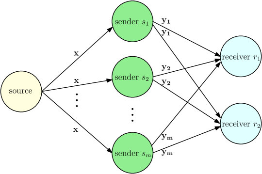
Refer to caption

Figure 2: The strategic communication system consisting of m𝑚m senders labeled as s1,,smsubscript𝑠1subscript𝑠𝑚s_{1},\!\cdots\!,s_{m} and 222 receivers labeled as r1subscript𝑟1r_{1} and r2subscript𝑟2r_{2}.

In this section we illustrate the extension of techniques from previous sections to a game with multiple receivers as shown in Fig. 2. We derive our results to the case with 2 receivers and note that our results can be extended to d>2𝑑2d>2 receivers easily.

More precisely, consider an m+2𝑚2m+2 player static game with m𝑚m senders and 2 receivers each with their own objectives that depend on a random state 𝒙𝒙\bm{x} sampled from a zero mean Gaussian distribution with positive-definite covariance ΣxsubscriptΣ𝑥\Sigma_{x}, i.e., 𝒙(0,Σx)similar-to𝒙0subscriptΣ𝑥\bm{x}\sim\mathbb{N}(0,\Sigma_{x}), and actions of the receivers r1subscript𝑟1r_{1} and r2subscript𝑟2r_{2} are denoted by 𝒖1subscript𝒖1\bm{u}_{1} and 𝒖2subscript𝒖2\bm{u}_{2}, respectively. Here, each player i𝑖i where i{s1,,sm,r1,r2}𝑖subscript𝑠1subscript𝑠𝑚subscript𝑟1subscript𝑟2i\in\{s_{1},\ldots,s_{m},r_{1},r_{2}\} has its own expected cost function given by

Ji({ηsj}j[m];γr1,γr2)=𝔼[Li(𝒙;𝒖𝟏=γr1(Ir1);𝒖𝟐=γr2(Ir2))]=𝔼[Qi𝒙+Ri1𝒖1+Ri2𝒖22].\displaystyle J_{i}(\{\eta_{s_{j}}\}_{j\in[m]};\gamma_{r_{1}},\gamma_{r_{2}})=\mathbb{E}[L_{i}(\bm{x};\bm{u_{1}}=\gamma_{r_{1}}(I_{r_{1}});\bm{u_{2}}=\gamma_{r_{2}}(I_{r_{2}}))]=\mathbb{E}\left[\left\|Q_{i}\bm{x}+R_{i1}\bm{u}_{1}+R_{i2}\bm{u}_{2}\right\|^{2}\right]. (60)

Here, similar to the previous sections, we denote by Li(𝒙;𝒖𝟏=γr1(Ir1);𝒖𝟐=γr2(Ir2))=Qi𝒙+Ri1𝒖1+Ri2𝒖22L_{i}(\bm{x};\bm{u_{1}}=\gamma_{r_{1}}(I_{r_{1}});\bm{u_{2}}=\gamma_{r_{2}}(I_{r_{2}}))=\left\|Q_{i}\bm{x}+R_{i1}\bm{u}_{1}+R_{i2}\bm{u}_{2}\right\|^{2} the cost function of player i𝑖i where Ir1=Ir2={𝒚1,,𝒚m}subscript𝐼subscript𝑟1subscript𝐼subscript𝑟2subscript𝒚1subscript𝒚𝑚I_{r_{1}}=I_{r_{2}}=\{\bm{y}_{1},\ldots,\bm{y}_{m}\} are the information structure of the receivers r1subscript𝑟1r_{1} and r2subscript𝑟2r_{2}, and ηsj()subscript𝜂subscript𝑠𝑗\eta_{s_{j}}(\cdot) is the strategy of sender sjsubscript𝑠𝑗s_{j} for j[m]𝑗delimited-[]𝑚j\in[m] and γr1()subscript𝛾subscript𝑟1\gamma_{r_{1}}(\cdot), γr2()subscript𝛾subscript𝑟2\gamma_{r_{2}}(\cdot) are strategies of receivers r1subscript𝑟1r_{1} and r2subscript𝑟2r_{2}, respectively. The game proceeds as in the previous sections where all the senders simultaneously commit to their own strategy followed by the receivers’ best responding to the committed senders’ strategies. Due to the presence of multiple receivers whose actions possibly affect each other as reflected in utilities given by (60), the receivers in turn play a Nash game among themselves after observing the senders’ commitments. Thus, a policy tuple ({ηsj}j[m],γ1,γ2)subscriptsubscriptsuperscript𝜂subscript𝑠𝑗𝑗delimited-[]𝑚superscriptsubscript𝛾1superscriptsubscript𝛾2(\{\eta^{*}_{s_{j}}\}_{j\in[m]},\gamma_{1}^{*},\gamma_{2}^{*}) is said to be in an equilibrium if

Ji(ηi,ηi,{γrk(ηi,ηi)}k[2])Ji(ηi,ηi,{γrk(ηi,ηi)}k[2]),ηiΩ,i{s1,,sm},formulae-sequencesubscript𝐽𝑖superscriptsubscript𝜂𝑖superscriptsubscript𝜂𝑖subscriptsuperscriptsubscript𝛾subscript𝑟𝑘superscriptsubscript𝜂𝑖superscriptsubscript𝜂𝑖𝑘delimited-[]2subscript𝐽𝑖subscript𝜂𝑖superscriptsubscript𝜂𝑖subscriptsuperscriptsubscript𝛾subscript𝑟𝑘subscript𝜂𝑖superscriptsubscript𝜂𝑖𝑘delimited-[]2formulae-sequencefor-allsubscript𝜂𝑖Ωfor-all𝑖subscript𝑠1subscript𝑠𝑚\displaystyle J_{i}(\eta_{i}^{*},\eta_{-i}^{*},\!\{\gamma_{r_{k}}^{*}(\eta_{i}^{*},\eta_{-i}^{*})\}_{k\in[2]})\!\leq\!J_{i}(\eta_{i},\eta_{-i}^{*},\!\{\gamma_{r_{k}}^{*}(\eta_{i},\eta_{-i}^{*})\}_{k\in[2]}),~{}\forall\eta_{i}\in\Omega,~{}\forall i\in\{s_{1},\ldots,s_{m}\},\!\! (61)
Ji({ηsj}j[m],γi({ηsj}j[m]),γi({ηsj}j[m]))Ji({ηsj}j[m],γi({ηsj}j[m]),γi({ηsj}j[m])),subscript𝐽𝑖subscriptsubscript𝜂subscript𝑠𝑗𝑗delimited-[]𝑚superscriptsubscript𝛾𝑖subscriptsubscript𝜂subscript𝑠𝑗𝑗delimited-[]𝑚superscriptsubscript𝛾𝑖subscriptsubscript𝜂subscript𝑠𝑗𝑗delimited-[]𝑚subscript𝐽𝑖subscriptsubscript𝜂subscript𝑠𝑗𝑗delimited-[]𝑚subscript𝛾𝑖subscriptsubscript𝜂subscript𝑠𝑗𝑗delimited-[]𝑚superscriptsubscript𝛾𝑖subscriptsubscript𝜂subscript𝑠𝑗𝑗delimited-[]𝑚\displaystyle J_{i}(\{\eta_{s_{j}}\}_{j\in[m]},\gamma_{i}^{*}(\{\eta_{s_{j}}\}_{j\in[m]}),\gamma_{-i}^{*}(\{\eta_{s_{j}}\}_{j\in[m]}))\leq J_{i}(\{\eta_{s_{j}}\}_{j\in[m]},\gamma_{i}(\{\eta_{s_{j}}\}_{j\in[m]}),\gamma_{-i}^{*}(\{\eta_{s_{j}}\}_{j\in[m]})), (62)

where γiΓsubscript𝛾𝑖Γ\gamma_{i}\in\Gamma for i{r1,r2}.𝑖subscript𝑟1subscript𝑟2i\in\{r_{1},r_{2}\}. In order to construct such an equilibrium tuple, we first need to analyze the Nash game played among the receivers for fixed senders’ strategies {ηsj}j[m]subscriptsubscript𝜂subscript𝑠𝑗𝑗delimited-[]𝑚\{\eta_{s_{j}}\}_{j\in[m]}.

For fixed senders’ strategies, receivers’ play a Nash game with utilities which are strictly convex in their action variables, since RrRrsuperscriptsubscript𝑅subscript𝑟topsubscript𝑅subscript𝑟R_{{r_{\ell}}\ell}^{\top}R_{{r_{\ell}}\ell} is assumed to be of full rank for all [2]delimited-[]2\ell\in[2]. Thus, in order to determine the NE of this strictly convex quadratic game among receivers, by differentiating each receiver’s cost function, we find the best response dynamics of each receiver for given senders’ strategies and the action of the other receiver. This leads to a set of necessary and sufficient conditions for 𝒖issuperscriptsubscript𝒖𝑖𝑠\bm{u}_{i}^{\prime}s to be in equilibrium due to strict convexity [37]. Thus, we obtain

R𝒖=𝒒,𝑅𝒖𝒒\displaystyle R\bm{u}=-\bm{q}, (63)

where 𝒖=[𝒖1,𝒖2]𝒖superscriptsuperscriptsubscript𝒖1topsuperscriptsubscript𝒖2toptop\bm{u}=[\bm{u}_{1}^{\top},\bm{u}_{2}^{\top}]^{\top}, 𝒙^=𝔼[𝒙|𝒚1,,𝒚m]^𝒙𝔼delimited-[]conditional𝒙subscript𝒚1subscript𝒚𝑚\hat{\bm{x}}=\mathbb{E}[\bm{x}|\bm{y}_{1},\ldots,\bm{y}_{m}], and

R=𝑅absent\displaystyle R= [Rr11Rr11Rr11Rr12Rr22Rr21Rr22Rr22],matrixsuperscriptsubscript𝑅subscript𝑟11topsubscript𝑅subscript𝑟11superscriptsubscript𝑅subscript𝑟11topsubscript𝑅subscript𝑟12superscriptsubscript𝑅subscript𝑟22topsubscript𝑅subscript𝑟21superscriptsubscript𝑅subscript𝑟22topsubscript𝑅subscript𝑟22\displaystyle\begin{bmatrix}R_{r_{1}1}^{\top}R_{r_{1}1}&R_{r_{1}1}^{\top}R_{r_{1}2}\\ R_{r_{2}2}^{\top}R_{r_{2}1}&R_{r_{2}2}^{\top}R_{r_{2}2}\\ \end{bmatrix}, (64)
𝒒=𝒒absent\displaystyle\bm{q}= [𝒙^Qr1Rr11,𝒙^Qr2Rr22].superscriptmatrixsuperscriptbold-^𝒙topsuperscriptsubscript𝑄subscript𝑟1topsubscript𝑅subscript𝑟11superscriptbold-^𝒙topsuperscriptsubscript𝑄subscript𝑟2topsubscript𝑅subscript𝑟22top\displaystyle\begin{bmatrix}\bm{\hat{x}}^{\top}Q_{r_{1}}^{\top}R_{r_{1}1},&\bm{\hat{x}}^{\top}Q_{r_{2}}^{\top}R_{r_{2}2}\end{bmatrix}^{\top}. (65)
Proposition 6

The 222-receiver quadratic game admits a unique solution when R𝑅R given in (64) is invertible. This unique NE solution is given by

𝒖=R1𝒒:=[K1𝒙^,K2𝒙^],superscript𝒖superscript𝑅1𝒒assignmatrixsubscript𝐾1bold-^𝒙subscript𝐾2bold-^𝒙\displaystyle\bm{u}^{*}=-R^{-1}\bm{q}:=\begin{bmatrix}-K_{1}\bm{\hat{x}},\\ -K_{2}\bm{\hat{x}}\end{bmatrix},

where 𝐪𝐪\bm{q} is provided in (65).

We note from (65) and Proposition 6 that at NE, each receiver’s best response is linear in the posterior estimate 𝒙^^𝒙\hat{\bm{x}}. This specific structure allows us to use tools similar to those in previous sections to find the NE among the senders. Considering the receivers’ NE policy given in Proposition 6, senders play a Nash game in the space of posteriors.

Next, we find the NE policies for senders. Senders want to minimize their own cost functions given by

minηiΩ𝔼[Qi𝒙+k=12RikKk𝒙^2],i{s1,,sm}.subscriptsubscript𝜂𝑖Ω𝔼delimited-[]superscriptnormsubscript𝑄𝑖𝒙superscriptsubscript𝑘12subscript𝑅𝑖𝑘subscript𝐾𝑘^𝒙2for-all𝑖subscript𝑠1subscript𝑠𝑚\displaystyle\min_{\eta_{i}\in\Omega}\mathbb{E}\left[\left\|Q_{i}\bm{x}+\sum_{k=1}^{2}R_{ik}K_{k}\hat{\bm{x}}\right\|^{2}\right],\quad\forall i\in\{s_{1},\dots,s_{m}\}. (66)

Thus, utilizing techniques from Section III, we can rewrite the objective function of each sender in (66) as

minηiΩTr(ViS),subscriptsubscript𝜂𝑖Ω𝑇𝑟subscript𝑉𝑖𝑆\displaystyle\min_{\eta_{i}\in\Omega}Tr(V_{i}S), (67)

where S=𝔼[𝒙^𝒙^]𝑆𝔼delimited-[]^𝒙superscript^𝒙topS=\mathbb{E}[\hat{\bm{x}}\hat{\bm{x}}^{\top}] and Visubscript𝑉𝑖V_{i} is given by

Vi=subscript𝑉𝑖absent\displaystyle V_{i}= K1Ri1Ri2K2+K2Ri2Ri1K1+K1Ri1Ri1K1+K2Ri2Ri2K2superscriptsubscript𝐾1topsuperscriptsubscript𝑅𝑖1topsubscript𝑅𝑖2subscript𝐾2superscriptsubscript𝐾2topsuperscriptsubscript𝑅𝑖2topsubscript𝑅𝑖1subscript𝐾1superscriptsubscript𝐾1topsuperscriptsubscript𝑅𝑖1topsubscript𝑅𝑖1subscript𝐾1superscriptsubscript𝐾2topsuperscriptsubscript𝑅𝑖2topsubscript𝑅𝑖2subscript𝐾2\displaystyle K_{1}^{\top}R_{i1}^{\top}R_{i2}K_{2}+K_{2}^{\top}R_{i2}^{\top}R_{i1}K_{1}+K_{1}^{\top}R_{i1}^{\top}R_{i1}K_{1}+K_{2}^{\top}R_{i2}^{\top}R_{i2}K_{2}
K1Ri1QiK2Ri2QiQiRi1K1QiRi2K2,i{s1,,sm}.superscriptsubscript𝐾1topsuperscriptsubscript𝑅𝑖1topsubscript𝑄𝑖superscriptsubscript𝐾2topsubscript𝑅𝑖2subscript𝑄𝑖superscriptsubscript𝑄𝑖topsuperscriptsubscript𝑅𝑖1topsubscript𝐾1superscriptsubscript𝑄𝑖topsubscript𝑅𝑖2subscript𝐾2𝑖subscript𝑠1subscript𝑠𝑚\displaystyle-K_{1}^{\top}R_{i1}^{\top}Q_{i}-K_{2}^{\top}R_{i2}Q_{i}-Q_{i}^{\top}R_{i1}^{\top}K_{1}-Q_{i}^{\top}R_{i2}K_{2},\quad i\in\{s_{1},\dots,s_{m}\}. (68)

We note that even in the presence of multiple receivers, senders’ Nash game can be written in terms of a trace minimization. Thus, we can utilize Algorithm 3 to identify stable posteriors which are achievable by using linear strategies as proved in Theorem 3.

VI Numerical Results

In this section, we provide simulation results to analyze the effects of multiple senders in the communication game across various settings. In the first 3 numerical results, we consider two senders and a single receiver and a state of the world given by 𝒙=[zθAθB]𝒙superscriptmatrix𝑧subscript𝜃𝐴subscript𝜃𝐵top\bm{x}=\begin{bmatrix}z&\theta_{A}&\theta_{B}\end{bmatrix}^{\top}. For all these examples, we consider quadratic cost functions for the players as noted below:

J1subscript𝐽1\displaystyle J_{1} =𝔼[(z+βθA+αθBu)2],absent𝔼delimited-[]superscript𝑧𝛽subscript𝜃𝐴𝛼subscript𝜃𝐵𝑢2\displaystyle=\mathbb{E}[(z+\beta\theta_{A}+\alpha\theta_{B}-u)^{2}], (69)
J2subscript𝐽2\displaystyle J_{2} =𝔼[(z+αθA+βθBu)2],absent𝔼delimited-[]superscript𝑧𝛼subscript𝜃𝐴𝛽subscript𝜃𝐵𝑢2\displaystyle=\mathbb{E}[(z+\alpha\theta_{A}+\beta\theta_{B}-u)^{2}], (70)
Jrsubscript𝐽𝑟\displaystyle J_{r} =𝔼[(zu)2],absent𝔼delimited-[]superscript𝑧𝑢2\displaystyle=\mathbb{E}[(z-u)^{2}], (71)

where we specify α𝛼\alpha and β𝛽\beta values for each example.131313Here, the actions are generated by policies/strategies as in Section II, but we suppress this representation throughout this section. We note that both senders having access to the full state allows us to have such objectives for the sender which depend on both θA,subscript𝜃𝐴\theta_{A}, θBsubscript𝜃𝐵\theta_{B}.141414In the first 3 numerical results, one could consider a more general model where α𝛼\alpha and β𝛽\beta could also be sender specific such that the expected cost functions are given by J1=𝔼[(z+β1θA+α1θBu)2]subscript𝐽1𝔼delimited-[]superscript𝑧subscript𝛽1subscript𝜃𝐴subscript𝛼1subscript𝜃𝐵𝑢2J_{1}=\mathbb{E}[(z+\beta_{1}\theta_{A}+\alpha_{1}\theta_{B}-u)^{2}] and J2=𝔼[(z+α2θA+β2θBu)2]subscript𝐽2𝔼delimited-[]superscript𝑧subscript𝛼2subscript𝜃𝐴subscript𝛽2subscript𝜃𝐵𝑢2J_{2}=\mathbb{E}[(z+\alpha_{2}\theta_{A}+\beta_{2}\theta_{B}-u)^{2}].

VI-1 Construction of Nash equilibrium policies

We first consider α=0𝛼0\alpha=0, and β=1𝛽1\beta=1, i.e., sender 111 has a quadratic cost to minimize 𝔼[(z+θAu)2]𝔼delimited-[]superscript𝑧subscript𝜃𝐴𝑢2\mathbb{E}[(z+\theta_{A}-u)^{2}] while sender 222 wants to minimize 𝔼[(z+θBu)2]𝔼delimited-[]superscript𝑧subscript𝜃𝐵𝑢2\mathbb{E}[(z+\theta_{B}-u)^{2}] and the receiver wants to minimize 𝔼[(zu)2]𝔼delimited-[]superscript𝑧𝑢2\mathbb{E}[(z-u)^{2}]. We consider a zero-mean Gaussian prior on the state of the world with the covariance matrix ΣxsubscriptΣ𝑥\Sigma_{x} given by

Σx=[10.50.70.51.50.20.70.21].subscriptΣ𝑥matrix10.50.70.51.50.20.70.21\displaystyle\Sigma_{x}=\begin{bmatrix}1&0.5&0.7\\ 0.5&1.5&0.2\\ 0.7&0.2&1\end{bmatrix}. (72)

By using Algorithm 2 to compute stable equilibrium posterior, we get

Σ=[0.97150.55710.77930.55711.38590.04130.77930.04130.7794],superscriptΣmatrix0.97150.55710.77930.55711.38590.04130.77930.04130.7794\displaystyle\Sigma^{*}=\begin{bmatrix}0.9715&0.5571&0.7793\\ 0.5571&1.3859&0.0413\\ 0.7793&0.0413&0.7794\end{bmatrix}, (73)

which achieves a NE expected cost values of J1=1.4144subscript𝐽11.4144J_{1}=1.4144, J2=0.8699subscript𝐽20.8699J_{2}=0.8699, and Jr=0.0285subscript𝐽𝑟0.0285J_{r}=0.0285 for senders 1 and 2, and the receiver, respectively. From Theorem 1, we can construct NE policies to be η1(𝒙)=η2(𝒙)=L𝒙subscript𝜂1𝒙subscript𝜂2𝒙𝐿𝒙\eta_{1}(\bm{x})=\eta_{2}(\bm{x})=L\bm{x}, where

L=[0000.10460.74210.57140.78070.18680.1464].𝐿matrix0000.10460.74210.57140.78070.18680.1464\displaystyle L=\begin{bmatrix}0&0&0\\ 0.1046&-0.7421&0.5714\\ -0.7807&-0.1868&-0.1464\end{bmatrix}.

As a sanity check we can see that such policies would return the equilibrium posterior ΣL=ΣxL(LΣxL)LΣx=ΣsubscriptΣ𝐿subscriptΣ𝑥superscript𝐿topsuperscript𝐿subscriptΣ𝑥superscript𝐿top𝐿subscriptΣ𝑥superscriptΣ\Sigma_{L}=\Sigma_{x}L^{\top}(L\Sigma_{x}L^{\top})^{\dagger}L\Sigma_{x}=\Sigma^{*} as given by (73).

VI-2 Correlation between the state of the world parameters

In the second numerical example, we consider the same setting as in the first example, i.e., α=0𝛼0\alpha=0, and β=1𝛽1\beta=1, but with a different covariance matrix ΣxsubscriptΣ𝑥\Sigma_{x}. Here, we take

Σx=[10.50.50.51ρab0.5ρab1],subscriptΣ𝑥matrix10.50.50.51subscript𝜌𝑎𝑏0.5subscript𝜌𝑎𝑏1\displaystyle\Sigma_{x}=\begin{bmatrix}1&0.5&0.5\\ 0.5&1&\rho_{ab}\\ 0.5&\rho_{ab}&1\end{bmatrix}, (74)

where ρabsubscript𝜌𝑎𝑏\rho_{ab} is the correlation coefficient between θAsubscript𝜃𝐴\theta_{A} and θBsubscript𝜃𝐵\theta_{B} which is given by ρab=Cov(θA,θB)Var(θA)Var(θB)subscript𝜌𝑎𝑏𝐶𝑜𝑣subscript𝜃𝐴subscript𝜃𝐵𝑉𝑎𝑟subscript𝜃𝐴𝑉𝑎𝑟subscript𝜃𝐵\rho_{ab}=\frac{Cov(\theta_{A},\theta_{B})}{\sqrt{Var(\theta_{A})Var(\theta_{B})}}. In this example, we vary ρab={0.5,0.4,,0.9}subscript𝜌𝑎𝑏0.50.40.9\rho_{ab}=\{-0.5,-0.4,\cdots,0.9\} and find the expected costs of the receiver and the senders obtained by Algorithms 1 and 2. In Fig. 3(a), we see how the error covariance of the receiver, i.e., Jr=𝔼[(zu)2]subscript𝐽𝑟𝔼delimited-[]superscript𝑧𝑢2J_{r}=\mathbb{E}[({z}-{u})^{2}], changes with respect to ρabsubscript𝜌𝑎𝑏\rho_{ab}. When ρab<0subscript𝜌𝑎𝑏0\rho_{ab}<0, θAsubscript𝜃𝐴\theta_{A}, and θBsubscript𝜃𝐵\theta_{B} are negatively correlated, and as a result, senders reveal more information to the receiver about the state of the world 𝒛𝒛\bm{z}. As the correlation ρabsubscript𝜌𝑎𝑏\rho_{ab} increases, the information revealed to the receiver decreases and the expected cost of the receiver Jrsubscript𝐽𝑟J_{r} increases. In Fig. 3(b), we see how the expected costs of the senders changes with respect to ρabsubscript𝜌𝑎𝑏\rho_{ab}. As the senders’ goals become aligned, they can manipulate the receiver more, and decrease their expected costs effectively. In Figs. 3(a)-(b), as both Algorithms 1 and 2 give the same equilibrium posteriors, we see that they achieve the same expected costs for the receiver and for the senders.
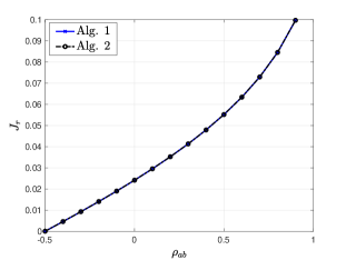
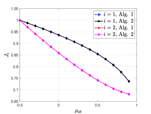
Refer to caption
Refer to caption
Figure 3: The expected costs of the (a) receiver, (b) sender i𝑖i for i={1,2}𝑖12i=\{1,2\} with respect to correlation coefficient ρabsubscript𝜌𝑎𝑏\rho_{ab}.

VI-3 Correlation between senders’ objectives

In the third numerical example, we consider ΣxsubscriptΣ𝑥\Sigma_{x} as in (74) with ρab=0.25subscript𝜌𝑎𝑏0.25\rho_{ab}=0.25. In this example, we take β=1𝛽1\beta=1 and vary α[1,1]𝛼11\alpha\in[-1,1]. Thus, the senders’ objective functions include both the parameters θAsubscript𝜃𝐴{\theta_{A}} and θBsubscript𝜃𝐵{\theta_{B}} where we have J1=𝔼[(z+θA+αθBu)2]subscript𝐽1𝔼delimited-[]superscript𝑧subscript𝜃𝐴𝛼subscript𝜃𝐵𝑢2J_{1}=\mathbb{E}[({z}+{\theta_{A}}+\alpha{\theta_{B}}-{u})^{2}] and J2=𝔼[(z+αθA+θBu)2]subscript𝐽2𝔼delimited-[]superscript𝑧𝛼subscript𝜃𝐴subscript𝜃𝐵𝑢2J_{2}=\mathbb{E}[({z}+\alpha{\theta_{A}}+{\theta_{B}}-{u})^{2}]. In this example, α𝛼\alpha represents the alignment of interests in θAsubscript𝜃𝐴\theta_{A}, θBsubscript𝜃𝐵\theta_{B} for the senders. As in the previous examples, the receiver is only interested in z𝑧z and thus, it has the objective function Jr=𝔼[(zu)2]subscript𝐽𝑟𝔼delimited-[]superscript𝑧𝑢2J_{r}=\mathbb{E}[({z}-{u})^{2}]. We see in Fig. 4(a) that when α=1𝛼1\alpha=-1, i.e., when the senders’ interests are exactly mismatched, the receiver can use this to its advantage and recover z𝑧{z} perfectly and thus, Jr=0subscript𝐽𝑟0J_{r}=0 when α=1𝛼1\alpha=-1. As α𝛼\alpha increases, the correlation between the senders’ objectives increases. As a result, the receiver gets less information about the parameter z𝑧{z}, and its expected cost Jrsubscript𝐽𝑟J_{r} increases with α𝛼\alpha. When there is an exact mismatch between the senders’ interests, i.e., when α=1𝛼1\alpha=-1, we see in Fig. 4(b) that the senders’ expected costs are high, as the receiver can recover z𝑧{z} perfectly. As α𝛼\alpha gets closer to 0, the senders’ objective functions become less dependent, and as a result, senders can achieve their minimum expected costs. As the senders’ objective functions are positively correlated, i.e., when α>0𝛼0\alpha>0, the expected cost is increasing for both senders.
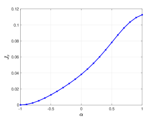
Refer to caption
Refer to caption
Figure 4: The expected costs of the (a) receiver, (b) sender i𝑖i for i={1,2}𝑖12i=\{1,2\} with respect to α𝛼\alpha.

VI-4 The effect of increasing the number of senders

In the fourth numerical example, we see the effect of increasing the number of senders m𝑚m on the expected costs of the receiver and sender 111. Let 𝒙=[z,θ1,,θm]𝒙superscriptmatrix𝑧subscript𝜃1subscript𝜃𝑚top\bm{x}=\begin{bmatrix}{z},&{\theta_{1}},\cdots,&{\theta_{m}}\end{bmatrix}^{\top}. The sender i𝑖i has the objective Ji=𝔼[(z+θiu)2]subscript𝐽𝑖𝔼delimited-[]superscript𝑧subscript𝜃𝑖𝑢2J_{i}=\mathbb{E}[({z}+{\theta_{i}}-{u})^{2}] for i=1,,m𝑖1𝑚i=1,\cdots,m and the receiver is only interested in z𝑧{z}, and thus has the objective function Jr=𝔼[(zu)2]subscript𝐽𝑟𝔼delimited-[]superscript𝑧𝑢2J_{r}=\mathbb{E}[({z}-{u})^{2}]. With these objective functions, we have the following matrices

Q1subscript𝑄1\displaystyle Q_{1} =[1100],R1=1,formulae-sequenceabsentmatrix1100subscript𝑅11\displaystyle=\begin{bmatrix}1&1&0&\cdots&0\end{bmatrix},\quad R_{1}=-1,
Q2subscript𝑄2\displaystyle Q_{2} =[1010],R2=1,formulae-sequenceabsentmatrix1010subscript𝑅21\displaystyle=\begin{bmatrix}1&0&1&\cdots&0\end{bmatrix},\quad R_{2}=-1,
\displaystyle\vdots Ri=1,subscript𝑅𝑖1\displaystyle\qquad\qquad\quad\vdots\qquad\qquad\quad\hskip 2.84526ptR_{i}=-1,
Qmsubscript𝑄𝑚\displaystyle Q_{m} =[1001],Rm=1,formulae-sequenceabsentmatrix1001subscript𝑅𝑚1\displaystyle=\begin{bmatrix}1&0&0&\cdots&1\end{bmatrix},\quad R_{m}=-1,
Qrsubscript𝑄𝑟\displaystyle Q_{r} =[1000],Rr=1.formulae-sequenceabsentmatrix1000subscript𝑅𝑟1\displaystyle=\begin{bmatrix}1&0&0&\cdots&0\end{bmatrix},\quad R_{r}=-1.

Then, we can find the corresponding Visubscript𝑉𝑖V_{i} matrices by using (9). In this example, we consider the covariance matrix to be

Σx=[1ρρρρ100ρ001],subscriptΣ𝑥matrix1𝜌𝜌𝜌𝜌100𝜌001\displaystyle\Sigma_{x}=\begin{bmatrix}1&\rho&\rho&\dots&\rho\\ \rho&1&0&\dots&0\\ \vdots&\vdots&\vdots&\ddots&\vdots\\ \rho&0&0&\dots&1\\ \end{bmatrix},\qquad (75)

where each sender’s private information is independent from the other senders’ private information but they are correlated with the receiver’s target information z𝑧{z} with correlation coefficient ρ𝜌\rho. For this example, we increase the number of senders m𝑚m from 1 to 10. In Fig. 5, we plot the receiver’s and the first sender’s expected costs as functions of m𝑚m when ρ={0.01,0.1,0.25}𝜌0.010.10.25\rho=\{0.01,0.1,0.25\}. For all ρ𝜌\rho values, as we increase the number of senders m𝑚m, more information is revealed by the senders and as a result the receiver is able to fully recover the desired information 𝒛𝒛\bm{z} and the receiver’s expected cost Jrsubscript𝐽𝑟J_{r} reduces down to 0 as seen in Fig. 5. We see that as ρ𝜌\rho gets higher, the senders reveal more information to the receiver, and thus Jrsubscript𝐽𝑟J_{r} gets lower. Similarly, as we increase the number of senders, the receiver gets more information from the other senders about its desired information z𝑧{z}, it gets less manipulated by each sender, and as a result J1subscript𝐽1J_{1} increases. As the receiver fully recovers z𝑧{z}, the expected cost of sender 111 approaches to J1=𝔼[(z+θ1z)2]=𝔼[θ12]=1subscript𝐽1𝔼delimited-[]superscript𝑧subscript𝜃1𝑧2𝔼delimited-[]superscriptsubscript𝜃121J_{1}=\mathbb{E}[({z}+{\theta_{1}}-{z})^{2}]=\mathbb{E}[\theta_{1}^{2}]=1 for all ρ𝜌\rho values. We see from Fig. 5(b) that the receiver is able to decrease its cost efficiently when the correlation coefficient between z𝑧{z} and its private information θisubscript𝜃𝑖{\theta_{i}}, i.e., ρ𝜌\rho, decreases. In Fig. 6, we repeat the same example for ρ={0.01,0.1,0.25}𝜌0.010.10.25\rho=\{-0.01,-0.1,-0.25\}, i.e., when z𝑧{z} and θisubscript𝜃𝑖{\theta_{i}} are negatively correlated. We see in Fig. 6(a) that the receiver can fully recover its desired information z𝑧{z} and also the expected cost of sender 111, J1subscript𝐽1J_{1}, decreases as the correlation between z𝑧{z} and θisubscript𝜃𝑖{\theta_{i}}, i.e., ρ𝜌\rho, decreases.

Refer to caption
Refer to caption
Figure 5: The expected costs of the (a) receiver, (b) sender 111 with respect to the number of senders when ρ={0.01,0.1,0.25}𝜌0.010.10.25\rho=\{0.01,0.1,0.25\}.
Refer to caption
Refer to caption
Figure 6: The expected costs of the (a) receiver, (b) sender 111 with respect to the number of senders when ρ={0.01,0.1,0.25}𝜌0.010.10.25\rho=\{-0.01,-0.1,-0.25\}.
N𝒩¯𝑁¯𝒩N\in\bar{\mathcal{N}} in Algorithm 3 J1subscript𝐽1J_{1} J2subscript𝐽2J_{2} J3subscript𝐽3J_{3} i=1mJisuperscriptsubscript𝑖1𝑚subscript𝐽𝑖\sum_{i=1}^{m}J_{i} Jrsubscript𝐽𝑟J_{r}
N={3,2,1}𝑁321N=\{3,2,1\} 0.7590 0.85270.85270.8527 0.91910.91910.9191 2.53082.53082.5308 0.03480.03480.0348
N={3,1,2}𝑁312N=\{3,1,2\} 0.85270.85270.8527 0.7590 0.91910.91910.9191 2.53082.53082.5308 0.03480.03480.0348
N={2,3,1}𝑁231N=\{2,3,1\} 0.7590 0.91910.91910.9191 0.85270.85270.8527 2.53082.53082.5308 0.03480.03480.0348
N={2,1,3}𝑁213N=\{2,1,3\} 0.85270.85270.8527 0.91910.91910.9191 0.7590 2.53082.53082.5308 0.03480.03480.0348
N={1,3,2}𝑁132N=\{1,3,2\} 0.91910.91910.9191 0.7590 0.85270.85270.8527 2.53082.53082.5308 0.03480.03480.0348
N={1,2,3}𝑁123N=\{1,2,3\} 0.91910.91910.9191 0.85270.85270.8527 0.7590 2.53082.53082.5308 0.03480.03480.0348
Full revelation 111 111 111 333 00
TABLE I: The expected costs of the senders and receiver when we apply Algorithm 3 with different ordering of senders. The minimum value in each column is indicated with bold text.

VI-5 Nash equilibrium posteriors obtained from Algorithm 3

In the fifth numerical example, we compare the NE posteriors obtained by solving the sequential optimization problem with varying order of Vissuperscriptsubscript𝑉𝑖𝑠V_{i}^{\prime}s for optimization considered in Algorithm 3. First, we consider ΣxsubscriptΣ𝑥\Sigma_{x} in (75) with ρ=0.1𝜌0.1\rho=0.1 for m=3𝑚3m=3. The senders’ and the receiver’s objective functions are given by Ji=𝔼[(z+θiu)2]subscript𝐽𝑖𝔼delimited-[]superscript𝑧subscript𝜃𝑖𝑢2J_{i}=\mathbb{E}[({z}+{\theta_{i}}-u)^{2}] for i=1,2,3𝑖123i=1,2,3 and Jr=𝔼[(zu)2]subscript𝐽𝑟𝔼delimited-[]superscript𝑧𝑢2J_{r}=\mathbb{E}[({z}-u)^{2}], respectively. We run Algorithm 3 for 666 different possible orderings and find the NE posteriors. We summarize the results by considering expected costs of individual senders, total sum of their costs and the receiver’s expected cost in Table I. We see that since θisubscript𝜃𝑖\theta_{i} variables are independent and identically distributed (i.i.d.), changing the ordering of Vissuperscriptsubscript𝑉𝑖𝑠V_{i}^{\prime}s does not change the senders’ total and the receiver’s expected costs, i.e., i=1mJi=2.5308superscriptsubscript𝑖1𝑚subscript𝐽𝑖2.5308\sum_{i=1}^{m}J_{i}=2.5308 and Jr=0.0348subscript𝐽𝑟0.0348J_{r}=0.0348 for all N𝒩¯𝑁¯𝒩N\in\bar{\mathcal{N}}, respectively. On the other hand, the order in Algorithm 3 affects the sender’s individual cost. We see in the first row of Table I that when the sequential optimization problem is solved in the order of N={3,2,1}𝑁321N=\{3,2,1\}, then sender 333 has the highest cost (J3=0.9191subscript𝐽30.9191J_{3}=0.9191) whereas sender 111 has the lowest cost (J1=0.7590subscript𝐽10.7590J_{1}=0.7590). As we solve for SDP involving V1subscript𝑉1V_{1} at the last stage, it can achieve the lowest cost compared to other senders. We re-emphasize that this sequence of ordering Vissuperscriptsubscript𝑉𝑖𝑠V_{i}^{\prime}s is only to solve the optimization problem in Algorithm 3 but any of the resulting posteriors above are in NE and are partially informative.

N𝒩¯𝑁¯𝒩N\in\bar{\mathcal{N}} in Algorithm 3 J1subscript𝐽1J_{1} J2subscript𝐽2J_{2} J3subscript𝐽3J_{3} i=1mJisuperscriptsubscript𝑖1𝑚subscript𝐽𝑖\sum_{i=1}^{m}J_{i} Jrsubscript𝐽𝑟J_{r}
N={3,2,1}𝑁321N=\{3,2,1\} 0.92550.92550.9255 0.97460.97460.9746 0.99230.99230.9923 2.89252.89252.8925 0.0066
N={3,1,2}𝑁312N=\{3,1,2\} 0.96630.96630.9663 0.94240.94240.9424 0.98980.98980.9898 2.89852.89852.8985 0.00880.00880.0088
N={2,3,1}𝑁231N=\{2,3,1\} 0.9196 0.99130.99130.9913 0.97980.97980.9798 2.8907 0.00780.00780.0078
N={2,1,3}𝑁213N=\{2,1,3\} 0.96600.96600.9660 0.98660.98660.9866 0.9513 2.90402.90402.9040 0.01200.01200.0120
N={1,3,2}𝑁132N=\{1,3,2\} 0.98980.98980.9898 0.9407 0.97990.97990.9799 2.91052.91052.9105 0.00960.00960.0096
N={1,2,3}𝑁123N=\{1,2,3\} 0.98800.98800.9880 0.97370.97370.9737 0.95310.95310.9531 2.91472.91472.9147 0.01130.01130.0113
Full revelation 111 111 111 333 00
TABLE II: The expected costs of the senders and the receiver when we apply Algorithm 3 with different orderings for senders. The minimum value of each column is indicated with bold text.

Next, we consider the following prior ΣxsubscriptΣ𝑥\Sigma_{x}:

Σx=[1002.557.52.510050107.5001],subscriptΣ𝑥matrix1002.557.52.510050107.5001\displaystyle\Sigma_{x}=\begin{bmatrix}100&2.5&5&7.5\\ 2.5&1&0&0\\ 5&0&1&0\\ 7.5&0&0&1\\ \end{bmatrix},\qquad (76)

where the correlation coefficients are ρzθ1=0.25subscript𝜌𝑧subscript𝜃10.25\rho_{z\theta_{1}}=0.25, ρzθ2=0.5subscript𝜌𝑧subscript𝜃20.5\rho_{z\theta_{2}}=0.5, and ρzθ3=0.75subscript𝜌𝑧subscript𝜃30.75\rho_{z\theta_{3}}=0.75. In other words, the correlation between z𝑧z and θisubscript𝜃𝑖\theta_{i} is increasing with i𝑖i. Since θisubscript𝜃𝑖\theta_{i}s are not i.i.d. anymore, the order in Algorithm 3 changes the total expected costs of the senders and the receiver. We see in Table II that the receiver’s expected cost is minimized (maximized) when V3subscript𝑉3V_{3} is solved first (last) in Algorithm 3, i.e., when N={3,2,1}𝑁321N=\{3,2,1\} (N={2,1,3}𝑁213N=\{2,1,3\}), respectively. Additionally, for the senders, we observe that each one’s individual cost is minimized when its order is last in Algorithm 3. Thus, there is no equilibrium among those calculated by our algorithm that is preferred by all senders. However, their total expected cost, i.e., =1mJsuperscriptsubscript1𝑚subscript𝐽\sum_{\ell=1}^{m}J_{\ell}, is minimized when N={2,3,1}𝑁231N=\{2,3,1\} where the NE posterior also minimizes sender 111’s individual cost whereas it maximizes sender 222’s individual cost compared to other NE posteriors.

In both examples, we see in Tables I and II that NE policies that we obtain in this paper are nontrivial in the sense that compared to the full revelation type, which is also an equilibrium, we attain equilibria that are preferred by all senders.

VI-6 Cooperative vs non-cooperative games among senders

In the sixth numerical example, we consider the ΣxsubscriptΣ𝑥\Sigma_{x} in (75) for ρ=0.01𝜌0.01\rho=0.01. Our goal is to compare the expected costs of all the senders and the receiver when the senders are cooperative, i.e., each sender wants to minimize a global objective function which is the summation of individual cost functions of the senders, and when the senders are non-cooperative, and hence playing a Nash game, which is the setting in our work. In the cooperative game, the cost function for each sender is given by Ji==1m𝔼[(z+θu)2]subscript𝐽𝑖superscriptsubscript1𝑚𝔼delimited-[]superscript𝑧subscript𝜃𝑢2J_{i}=\sum_{\ell=1}^{m}\mathbb{E}[({z}+{\theta_{\ell}}-u)^{2}]. Similar to the derivations in (9), the objective function of each sender can be written as

minΣxΣ0Tr((=1mV)Σ).subscriptsucceeds-or-equalssubscriptΣ𝑥Σsucceeds-or-equals0𝑇𝑟superscriptsubscript1𝑚subscript𝑉Σ\displaystyle\min_{\Sigma_{x}\succeq\Sigma\succeq 0}Tr\left(\left(\sum_{\ell=1}^{m}V_{\ell}\right)\Sigma\right). (77)

Here, as the senders have the same global objective function, the optimal solution to (77) will minimize the expected cost of each sender. Thus, it is sufficient to solve the optimization problem in (77) just for a single sender. Then, we compare the cooperative game cost with the non-cooperative game setting where the senders have Ji=𝔼[(z+θiu)2]subscript𝐽𝑖𝔼delimited-[]superscript𝑧subscript𝜃𝑖𝑢2J_{i}=\mathbb{E}[({z}+{\theta_{i}}-u)^{2}] for i=1,,m𝑖1𝑚i=1,\dots,m, as in the fourth numerical example. In order to make a fair comparison, we compute i=1mJisuperscriptsubscript𝑖1𝑚subscript𝐽𝑖\sum_{i=1}^{m}J_{i} for the non-cooperative game, and compare it with the expected cost of the single sender objective function Ji==1m𝔼[(z+θu)2]subscript𝐽𝑖superscriptsubscript1𝑚𝔼delimited-[]superscript𝑧subscript𝜃𝑢2J_{i}=\sum_{\ell=1}^{m}\mathbb{E}[({z}+{\theta_{\ell}}-u)^{2}] in the cooperative game scenario. We see in Fig. 7(b) that cooperation among the senders helps reduce their total expected cost compared to the non-cooperative game setting. We note that the total expected cost of the senders increases linearly with m𝑚m. We see in Fig. 7(a) that the cooperation between the senders is not beneficial for the receiver as it gets less informative signals from the senders. However, the receiver’s expected cost decreases as the number of senders, m𝑚m, increases. Thus, even if the senders cooperate, having multiple senders can still be helpful for the receiver.
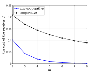
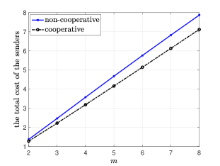
Refer to caption
Refer to caption
Figure 7: (a) The expected costs of the receiver, (b) the total cost of the senders when the senders are cooperative and non-cooperative.

VI-7 Dynamic information disclosure

In the seventh numerical example, we consider the multi-stage game with m=2𝑚2m=2 senders and n=10𝑛10n=10 stages where the 333-dimensional state of the world 𝒙𝒌=[zk,θAk,θBk]subscript𝒙𝒌subscript𝑧𝑘subscript𝜃subscript𝐴𝑘subscript𝜃subscript𝐵𝑘\bm{x_{k}}=[z_{k},\theta_{A_{k}},\theta_{B_{k}}] evolves over time as follows:

𝒙𝒌=A𝒙𝒌𝟏+𝒘𝒌𝟏,k{1,,n},formulae-sequencesubscript𝒙𝒌𝐴subscript𝒙𝒌1subscript𝒘𝒌1𝑘1𝑛\displaystyle\bm{x_{k}}=A\bm{x_{k-1}}+\bm{w_{k-1}},\quad k\in\{1,\dots,n\}, (78)

where A=I𝐴𝐼A=I, and 𝒙𝟎subscript𝒙0\bm{x_{0}} has a zero-mean Gaussian distribution with variance Σ0subscriptΣ0\Sigma_{0}, i.e., (0,Σ0)0subscriptΣ0\mathbb{N}(0,\Sigma_{0}), where

Σ0=[10.50.50.5100.501],subscriptΣ0matrix10.50.50.5100.501\displaystyle\Sigma_{0}=\begin{bmatrix}1&0.5&0.5\\ 0.5&1&0\\ 0.5&0&1\end{bmatrix},

and, wksubscript𝑤𝑘w_{k} has (0,Σw)0subscriptΣ𝑤\mathbb{N}(0,\Sigma_{w}) with Σw=IsubscriptΣ𝑤𝐼\Sigma_{w}=I. For this example, we consider the case where the objective functions of the senders are changing over each stage k𝑘k, denoted by Jiksuperscriptsubscript𝐽𝑖𝑘J_{i}^{k} and are given by

J1k=𝔼[(zk+knθAkuk)2],J2k=𝔼[(zk+nknθBkuk)2],k[n].formulae-sequencesuperscriptsubscript𝐽1𝑘𝔼delimited-[]superscriptsubscript𝑧𝑘𝑘𝑛subscript𝜃subscript𝐴𝑘subscript𝑢𝑘2formulae-sequencesuperscriptsubscript𝐽2𝑘𝔼delimited-[]superscriptsubscript𝑧𝑘𝑛𝑘𝑛subscript𝜃subscript𝐵𝑘subscript𝑢𝑘2for-all𝑘delimited-[]𝑛\displaystyle J_{1}^{k}=\mathbb{E}\left[\left({z_{k}}+\frac{k}{n}{\theta_{A_{k}}}-u_{k}\right)^{2}\right],\quad J_{2}^{k}=\mathbb{E}\left[\left({z_{k}}+\frac{n-k}{n}{\theta_{B_{k}}}-u_{k}\right)^{2}\right],\quad\forall k\in[n]. (79)

The receiver’s expected cost function at stage k𝑘k is given by Jrk=𝔼[(zkuk)2]superscriptsubscript𝐽𝑟𝑘𝔼delimited-[]superscriptsubscript𝑧𝑘subscript𝑢𝑘2J_{r}^{k}=\mathbb{E}[(z_{k}-u_{k})^{2}]. With these expected cost functions, we find Vkisuperscriptsubscript𝑉𝑘𝑖V_{k}^{i} in (55) as follows:

Vk1=[1kn0kn00000],Vk2=[10nkn000nkn00].formulae-sequencesuperscriptsubscript𝑉𝑘1matrix1𝑘𝑛0𝑘𝑛00000superscriptsubscript𝑉𝑘2matrix10𝑛𝑘𝑛000𝑛𝑘𝑛00\displaystyle V_{k}^{1}=\begin{bmatrix}-1&-\frac{k}{n}&0\\ -\frac{k}{n}&0&0\\ 0&0&0\end{bmatrix},\qquad V_{k}^{2}=\begin{bmatrix}-1&0&-\frac{n-k}{n}\\ 0&0&0\\ -\frac{n-k}{n}&0&0\end{bmatrix}.

In this example, based on (79), the objective function of sender 111 is initially aligned with that of the receiver whereas sender 222 has a more misaligned objective. As the time horizon k𝑘k gets closer to n𝑛n, we see that the objective of sender 111 becomes misaligned whereas sender 222’s objective function becomes aligned with that of the receiver. We plot the senders’ and the receiver’s cost functions at stage k𝑘k in Fig. 8. As seen in Fig. 8(a), the receiver is able to minimize its cost well when at least one sender has aligned objective functions with the receiver, which happens when k𝑘k is small and when k𝑘k is close to n𝑛n. We observe from Fig. 8(b) that sender 111’s expected cost is increasing with k𝑘k. As sender 111’s objective function diverges from the receiver’s objective, the receiver gets more reliable information from sender 222. Here, sender 222 is able to minimize its cost by revealing more information to the receiver as its objective function becomes more aligned as k𝑘k grows.

Refer to caption
Refer to caption
Figure 8: Dynamic information disclosure games with time horizon n=10𝑛10n=10 for m=2𝑚2m=2 senders the expected costs of (a) the receiver, (b) the senders.

VI-8 Multi-Sender Multi-Receiver

In the eighth numerical example, we first consider a single sender and 2 receivers, and a state of the world 𝒙=[z,θA,θB]𝒙superscript𝑧subscript𝜃𝐴subscript𝜃𝐵top\bm{x}=[z,\theta_{A},\theta_{B}]^{\top}, 𝒙=[zθAθB]𝒙superscriptmatrix𝑧subscript𝜃𝐴subscript𝜃𝐵top\bm{x}=\begin{bmatrix}z&\theta_{A}&\theta_{B}\end{bmatrix}^{\top}which has a zero-mean Gaussian prior with covariance matrix ΣxsubscriptΣ𝑥\Sigma_{x} given by

Σx=[10.50.50.510.250.50.251].subscriptΣ𝑥matrix10.50.50.510.250.50.251\displaystyle\Sigma_{x}=\begin{bmatrix}1&0.5&0.5\\ 0.5&1&0.25\\ 0.5&0.25&1\end{bmatrix}. (80)

The sender’s and the receivers’ cost functions are given by

Js1=𝔼[(z+θBu1+u22)2],Jr1=𝔼[(zu1αu2)2],Jr2=𝔼[(z+θAαu1u2)2].formulae-sequencesubscript𝐽subscript𝑠1𝔼delimited-[]superscript𝑧subscript𝜃𝐵subscript𝑢1subscript𝑢222formulae-sequencesubscript𝐽subscript𝑟1𝔼delimited-[]superscript𝑧subscript𝑢1𝛼subscript𝑢22subscript𝐽subscript𝑟2𝔼delimited-[]superscript𝑧subscript𝜃𝐴𝛼subscript𝑢1subscript𝑢22\displaystyle J_{s_{1}}=\mathbb{E}\left[\left(z+\theta_{B}-\frac{u_{1}+u_{2}}{2}\right)^{2}\right],~{}J_{r_{1}}\!=\!\mathbb{E}\left[\left(z-u_{1}-\alpha u_{2}\right)^{2}\right],~{}J_{r_{2}}\!=\!\mathbb{E}\left[\left(z+\theta_{A}\!-\!\alpha u_{1}\!-\!u_{2}\right)^{2}\right]. (81)

By using Proposition 6, we found the optimum receivers’ best response as

𝒖=[K1𝒙^K2𝒙^],superscript𝒖matrixsubscript𝐾1bold-^𝒙subscript𝐾2bold-^𝒙\displaystyle\bm{u}^{*}=\begin{bmatrix}-K_{1}\bm{\hat{x}}\\ -K_{2}\bm{\hat{x}}\end{bmatrix},

where K1=[1,α1α,0]subscript𝐾11𝛼1𝛼0K_{1}=[-1,\frac{\alpha}{1-\alpha},0] and K2=[1,11α,0]subscript𝐾2111𝛼0K_{2}=[-1,-\frac{1}{1-\alpha},0]. Then, we write the objective function of the sender in (67) as

minηΩTr(VS),subscript𝜂Ω𝑇𝑟𝑉𝑆\displaystyle\min_{\eta\in\Omega}Tr(VS), (82)

where S=𝔼[𝒙^𝒙^]𝑆𝔼delimited-[]^𝒙superscript^𝒙topS=\mathbb{E}[\hat{\bm{x}}\hat{\bm{x}}^{\top}] and

V=[101014121120].𝑉matrix101014121120\displaystyle V=\begin{bmatrix}-1&0&-1\\ 0&\frac{1}{4}&-\frac{1}{2}\\ -1&-\frac{1}{2}&0\end{bmatrix}. (83)

In this example, we vary α={0,0.1,,0.9}𝛼00.10.9\alpha=\{0,0.1,\dots,0.9\}, and find the optimum posterior induced by the sender S𝑆S, and then calculate the corresponding expected costs of players. We note that the sender’s objective function does not depend on the variable α𝛼\alpha. By using Algorithm 3, we find S𝑆S as

S=[0.8430.490.730.490.290.420.730.420.63],superscript𝑆matrix0.8430.490.730.490.290.420.730.420.63\displaystyle S^{*}=\begin{bmatrix}0.843&0.49&0.73\\ 0.49&0.29&0.42\\ 0.73&0.42&0.63\end{bmatrix}, (84)

the corresponding expected cost at the sender is given by Tr(VS)=0.3464𝑇𝑟𝑉superscript𝑆0.3464Tr(VS^{*})=0.3464. From Theorem 1, we can construct equilibrium policy to be η1(𝒙)=L𝒙subscript𝜂1𝒙𝐿𝒙\eta_{1}(\bm{x})=L\bm{x}, where

L=[0.64520.09930.4466000000].𝐿matrix0.64520.09930.4466000000\displaystyle L=\begin{bmatrix}-0.6452&-0.0993&-0.4466\\ 0&0&0\\ 0&0&0\end{bmatrix}.

The receivers’ expected costs are given in Fig. 9. As we increase α𝛼\alpha, the receivers’ objective functions start to couple with each other. As a result, their expected costs increases with α𝛼\alpha as shown in Fig. 9.

Refer to caption

Figure 9: The expected costs at the receivers for a system with a single sender and 2 receivers.

VII Discussion on Sequential Persuasion

In this section, we highlight an interesting property of the equilibrium obtained in the static multi-sender communication game. First, note that there can be multiple equilibrium definitions based on the times of commitment by the senders. Two of them considered in this paper include the NE (Theorem 1) due to simultaneous commitment among senders as stated in (3) and a sequential commitment with second sender entering the game between an existing sender and receiver as derived in Theorem 2. Although the posteriors obtained in both cases through Algorithm 2 are the same, the way that they are achieved is different due to the commitment order. Further, as stated in the text, NE in general for a multi-sender communication problem is not unique, and thus can result in multiple equilibrium posteriors. On the other hand, in the case of sequential commitment when the second sender enters an existing communication game as described in Theorem 2, the second sender faces an optimization problem which has essentially a unique solution, and thus resulting in a unique equilibrium posterior for this game. The fact that these two equilibrium posteriors can be obtained from the same algorithm boils down to the partially informative Nash equilibrium refinement as defined earlier.

Alternatively, one can consider a strictly sequential game between the senders where sender 111 moves first knowing that sender 222 would join the game in the next stage before the receiver takes an action. Since both senders have complete access to the state, any policy profile (η1,η2)subscript𝜂1subscript𝜂2(\eta_{1},\eta_{2}) of the senders can have an equivalent policy profile (η1,η2)superscriptsubscript𝜂1superscriptsubscript𝜂2(\eta_{1}^{\prime},\eta_{2}^{\prime}) such that η2superscriptsubscript𝜂2\eta_{2}^{\prime} does not add any additional information about the state [28]. This can be done by adding incentive compatibility constraints for sender 222 into sender 111’s optimization problem. Thus without loss of generality, sender 111’s optimization problem after following the simplification in (8) and by utilizing Lemma 2 becomes

minΣxS0subscriptsucceeds-or-equalssubscriptΣ𝑥𝑆succeeds-or-equals0\displaystyle\min_{\Sigma_{x}\succeq S\succeq 0}\quad Tr(V1S)𝑇𝑟subscript𝑉1𝑆\displaystyle Tr(V_{1}S)
s.t. (ΣxS)12V2(ΣxS)12O.succeeds-or-equalssuperscriptsubscriptΣ𝑥𝑆12subscript𝑉2superscriptsubscriptΣ𝑥𝑆12𝑂\displaystyle(\Sigma_{x}-S)^{\frac{1}{2}}V_{2}(\Sigma_{x}-S)^{\frac{1}{2}}\succeq O.

Due to the similarity between this objective and the steps in Algorithm 2, similar techniques can be used to obtain an equilibrium posterior. We leave this problem as a future research direction.

To summarize one key difference between sequential games and NE is that in sequential commitment the order of the senders matters and the equilibrium reached is essentially unique. Further, it can be seen that NE posteriors are at least as informative as sequential equilibrium posteriors. This is in line with the observation made in [28] for discrete state and action spaces.

VIII Conclusion and Future Direction

In this work, we have considered a strategic communication game problem between multiple senders and a receiver with misaligned objective functions. First, by focusing on the 2-sender case, we have posed the senders’ optimization problems in terms of the receiver’s posterior covariance. Then, by relaxing the constraint, we have proposed a sequential optimization technique to find the stable posteriors which can be achieved by using linear noiseless policies, and as a result they are in fact the equilibrium policies for the senders. Next, we have extended our solution to multiple senders (m>2𝑚2m>2) and characterized partially informative equilibrium posteriors, i.e., there exists no other more informative equilibrium which is beneficial for all the senders to deviate. Further, we have added dynamics to the problem by considering a Markovian evolution process of the underlying state with finite-horizon quadratic costs for the players. In this case we have shown that the equilibrium obtained by considering single-stage games is in fact stable and nontrivial. Finally, we extended the analysis to account for multiple receivers. Through extensive simulations, we have shown that having multiple senders is beneficial to the receiver as its estimation error cannot get worse by increasing the number of senders. It is also beneficial to the receiver to have senders with maximum misalignment between their objectives.

One immediate future direction of research is to explore the multi-stage case further, and characterize all possible equilibrium strategies. Further, we note that there might be other procedures (inspired by the approach in [33]) that can achieve equilibrium posteriors not obtained by our algorithms. We plan to investigate such procedures for achieving admissible equilibria[37] from which deviation to any other equilibrium is not profitable for any of the senders. Another promising direction is to consider the senders with private information where the private information is statistically known but its realization is not observable by the other players. It would be interesting to explore the effect of misalignment between sender objectives and verify if it still would be beneficial for the receiver to have multiple senders in all scenarios. Finally, it is crucial to understand the importance of equilibrium in linear policies. More precisely, it would be interesting to investigate if all the stable posteriors are achievable (or equivalently, identifying a necessary and sufficient condition for a posterior covariance to be an equilibrium posterior) using senders policies in some other policy class. In contrast with persuasion in the presence of a single sender, it is not obvious to achieve all stable posteriors using linear plus noise policies as in [35].

References

  • [1] I. Kostrikov, K. K. Agrawal, D. Dwibedi, S. Levine, and J. Tompson. Discriminator-actor-critic: Addressing sample inefficiency and reward bias in adversarial imitation learning. arXiv preprint arXiv:1809.02925, 2018.
  • [2] S. Arora and P. Doshi. A survey of inverse reinforcement learning: Challenges, methods and progress. Artificial Intelligence, 297:103500, 2021.
  • [3] A. N. Bhagoji, S. Chakraborty, P. Mittal, and S. Calo. Analyzing federated learning through an adversarial lens. In International Conference on Machine Learning, pages 634–643. PMLR, June 2019.
  • [4] A. Kashyap, T. Başar, and R. Srikant. Quantized consensus. Automatica, 43(7):1192–1203, 2007.
  • [5] P. Milgrom and J. Roberts. Relying on the information of interested parties. The RAND Journal of Economics, pages 18–32, 1986.
  • [6] V. P. Crawford and J. Sobel. Strategic information transmission. Econometrica: Journal of the Econometric Society, pages 1431–1451, 1982.
  • [7] A. Ambrus and S. Takahashi. Multi-sender cheap talk with restricted state spaces. Theoretical Economics, 2008.
  • [8] A. McGee and H. Yang. Cheap talk with two senders and complementary information. Games and Economic Behavior, 79:181–191, 2013.
  • [9] M. Ivanov. Communication via a strategic mediator. Journal of Economic Theory, 145(2):869–884, 2010.
  • [10] M. Ivanov. Dynamic information revelation in cheap talk. The BE Journal of Theoretical Economics, 15(2):251–275, 2015.
  • [11] S. Sarıtaş, S. Yüksel, and S. Gezici. Quadratic multi-dimensional signaling games and affine equilibria. IEEE Transactions on Automatic Control, 62(2):605–619, 2016.
  • [12] E. Kamenica and M. Gentzkow. Bayesian persuasion. American Economic Review, 101(6):2590–2615, 2011.
  • [13] L. Rayo and I. Segal. Optimal information disclosure. Journal of Political Economy, 118(5):949–987, 2010.
  • [14] R. J. Aumann, M. Maschler, and R. E. Stearns. Repeated Games with Incomplete Information. MIT Press, 1995.
  • [15] F. Farokhi, A. M. H. Teixeira, and C. Langbort. Estimation with strategic sensors. IEEE Transactions on Automatic Control, 62(2):724–739, 2016.
  • [16] S. Sarıtaş, S. Yüksel, and S. Gezici. Dynamic signaling games with quadratic criteria under Nash and Stackelberg equilibria. Automatica, 115:108883, 2020.
  • [17] J. Chen, M. Li, and H. Xu. Selling data to a machine learner: Pricing via costly signaling. In International Conference on Machine Learning, pages 3336–3359. PMLR, 2022.
  • [18] E. Akyol, C. Langbort, and T. Başar. Information-theoretic approach to strategic communication as a hierarchical game. Proceedings of the IEEE, 105(2):205–218, 2016.
  • [19] D. Bergemann and S. Morris. Information design: A unified perspective. Journal of Economic Literature, 57(1):44–95, 2019.
  • [20] S. Dughmi and H. Xu. Algorithmic Bayesian persuasion. In Proceedings of the forty-eighth annual ACM symposium on Theory of Computing, pages 412–425, 2016.
  • [21] J. C. Ely. Beeps. American Economic Review, 107(1):31–53, 2017.
  • [22] J. Renault, E. Solan, and N. Vieille. Optimal dynamic information provision. Games and Economic Behavior, 104:329–349, 2017.
  • [23] E. Kamenica. Bayesian persuasion and information design. Annual Review of Economics, 11:249–272, 2019.
  • [24] A. Fickinger, S. Zhuang, D. Hadfield-Menell, and S. Russell. Multi-principal assistance games. arXiv preprint arXiv:2007.09540, 2020.
  • [25] D. Martimort and L. Stole. The revelation and delegation principles in common agency games. Econometrica, 70(4):1659–1673, 2002.
  • [26] M. Gentzkow and E. Kamenica. Bayesian persuasion with multiple senders and rich signal spaces. Games and Economic Behavior, 104:411–429, 2017.
  • [27] M. Gentzkow and E. Kamenica. Competition in persuasion. The Review of Economic Studies, 84(1):300–322, 2016.
  • [28] F. Li and P. Norman. Sequential persuasion. Theoretical Economics, 16(2):639–675, 2021.
  • [29] W. Wu. Sequential Bayesian persuasion. ShanghaiTech SEM Working Paper, May 2021.
  • [30] Yun Wang. Bayesian persuasion with multiple receivers. Available at SSRN 2625399, 2013.
  • [31] Itai Arieli and Yakov Babichenko. Private Bayesian persuasion. Journal of Economic Theory, 182:185–217, 2019.
  • [32] Yakov Babichenko and Siddharth Barman. Computational aspects of private Bayesian persuasion. arXiv preprint arXiv:1603.01444, 2016.
  • [33] Wataru Tamura. Bayesian persuasion with quadratic preferences. Available at SSRN 1987877, 2018.
  • [34] M. O Sayin, E. Akyol, and T. Başar. Hierarchical multistage Gaussian signaling games in noncooperative communication and control systems. Automatica, 107:9–20, 2019.
  • [35] M. O. Sayin and T. Başar. Persuasion-based robust sensor design against attackers with unknown control objectives. IEEE Transactions on Automatic Control, 66(10):4589–4603, 2021.
  • [36] M. O. Sayin and T. Başar. Bayesian persuasion with state-dependent quadratic cost measures. IEEE Transactions on Automatic Control, 67(3):1241–1252, 2022.
  • [37] T. Başar and G. J. Olsder. Dynamic Noncooperative Game Theory. SIAM, 1998.
  • [38] J. Groß. Löwner partial ordering and space preordering of Hermitian non-negative definite matrices. Linear Algebra and its Applications, 326(1-3):215–223, 2001.
  • [39] J. Sobel. Giving and receiving advice. Advances in Economics and Econometrics, 1:305–341, 2013.
  • [40] W. Tamura. A theory of multidimensional information disclosure. Technical report, ISER Discussion Paper, 2012.
  • [41] M. Grant, S. Boyd, and Y. Ye. CVX: Matlab software for disciplined convex programming, 2008.
  • [42] B. Recht. A simpler approach to matrix completion. Journal of Machine Learning Research, 12(12), 2011.