Geometry-Aware Bandit Algorithms

Geometry-Aware Approaches for Balancing Performance and Theoretical Guarantees in Linear Bandits

Yuwei Luo Graduate School of Business, Stanford University, yuweiluo@stanford.edu Mohsen Bayati Graduate School of Business, Stanford University, bayati@stanford.edu

This paper is motivated by recent research in the $d$-dimensional stochastic linear bandit literature, which has revealed an unsettling discrepancy: algorithms like Thompson sampling and Greedy demonstrate promising empirical performance, yet this contrasts with their pessimistic theoretical regret bounds. The challenge arises from the fact that while these algorithms may perform poorly in certain problem instances, they generally excel in typical instances. To address this, we propose a new data-driven technique that tracks the geometric properties of the uncertainty ellipsoid around the main problem parameter. This methodology enables us to formulate an instance-dependent frequentist regret bound, which incorporates the geometric information, for a broad class of base algorithms, including Greedy, OFUL, and Thompson sampling. This result allows us to identify and “course-correct” problem instances in which the base algorithms perform poorly. The course-corrected algorithms achieve the minimax optimal regret of order $\widetilde{\mathcal{O}}(d\sqrt{T})$ for a $T$-period decision-making scenario, effectively maintaining the desirable attributes of the base algorithms, including their empirical efficacy. We present simulation results to validate our findings using synthetic and real data.

Linear bandit, Thompson sampling, Greedy, Data-driven exploration

1 Introduction

Multi-armed bandits (MABs) have garnered significant attention as they provide well-defined framework and techniques for investigating the exploration-exploitation trade-off in sequential decision-making problems. In the context of MAB problems, a decision-maker sequentially selects actions from a given set and observes corresponding rewards.

This paper focuses on the stochastic linear bandit (LB) model, which encompasses MAB and contextual bandit problems as special cases. In this model, the problem parameter $\theta^{\star}$ represents an unknown vector in $\mathbb{R}^{d}$, while the actions, also vectors in $\mathbb{R}^{d}$, yield noisy rewards with mean equal to the inner product of $\theta^{\star}$ and the chosen action. The objective of a policy is to maximize the cumulative reward based on the observed data up to the decision time. The policy’s performance is measured by the cumulative regret, which quantifies the difference between the total expected rewards achieved by the policy and the maximum achievable expected reward.

Achieving this objective necessitates striking a balance between exploration and exploitation. In the context of LB, this entails selecting actions that aid in estimating the true parameter $\theta^{\star}$ accurately while obtaining optimal rewards. Various algorithms based on the Optimism in the Face of Uncertainty (OFU) principle have been developed to address this challenge, wherein the optimal action is chosen based on the upper confidence bound (UCB) (Lai and Robbins, 1985; Auer, 2002; Dani et al., 2008; Rusmevichientong and Tsitsiklis, 2010). Another popular strategy is Thompson sampling (TS), a Bayesian heuristic introduced by Thompson (1933) that employs randomization to select actions according to the posterior distribution of reward functions. Additionally, the Greedy policy that selects the myopically best action is shown to be effective in contextual bandits (Kannan et al., 2018; Raghavan et al., 2018; Hao et al., 2020; Bastani et al., 2021).

In the linear bandit setting, two types of regret are considered. The Bayesian regret is applicable when the parameter $\theta^{\star}$ is random, and the regret is averaged over three sources of randomness: the observation noise, the randomized algorithm, and the random parameter $\theta^{\star}$. Russo and Van Roy (2014) and Dong and Van Roy (2018) establish an $\widetilde{\mathcal{O}}(d\sqrt{T})$ upper bound for the Bayesian regret of the TS heuristic referred to as LinTS, which matches the minimax optimal bound shown by Dani et al. (2008), where $\widetilde{\mathcal{O}}$ refers to asymptotic order, up to polylogarithmic factors.

On the other hand, the frequentist regret corresponds to scenarios where the underlying parameter $\theta^{\star}$ is fixed, and the expectation is taken only with respect to the randomness of the noise and the algorithm. In this frequentist setting, the optimism-based algorithm proposed by Abbasi-Yadkori et al. (2011), known as Optimism in the Face of Uncertainty Linear Bandit Algorithm (OFUL), achieves a $\widetilde{\mathcal{O}}(d\sqrt{T})$ frequentist regret bound, which matches the minimax optimal Bayesian bound. However, for a frequentist variant of LinTS referred to as TS-Freq, which inflates the posterior distribution, Agrawal and Goyal (2013) and Abeille et al. (2017) provide a $\widetilde{\mathcal{O}}(d\sqrt{dT})$ upper bound for the frequentist regret. This regret bound falls short of the optimal rate by a factor of $\sqrt{d}$. Recent work by Hamidi and Bayati (2020b) confirms that this inflation is necessary, and thus, the frequentist regret of LinTS cannot be improved. For the Greedy algorithm in linear bandit problems, no general theoretical guarantee exists. Moreover, it is known that both LinTS and Greedy might perform suboptimally in the asymptotic regime (Lattimore and Szepesvari, 2017).

Despite the theoretical gaps in performance, LinTS has shown strong empirical performance (Russo et al., 2018), indicating that the inflation of the posterior distribution may be unnecessary in most problem instances, and unfavorable instances are unlikely to occur frequently. Similarly, the Greedy algorithm works well in typical instances (Bietti et al., 2021). Additionally, while OFU-based algorithms are computationally expensive (generally NP-hard as discussed by Dani et al. (2008); Russo and Van Roy (2014); Agrawal (2019)), LinTS and Greedy are known for their computational efficiency. This unsettling disparity between theoretical, computational, and empirical performance has motivated our investigation into the following two questions: Is it possible to identify, in a data-driven fashion, problematic instances where LinTS and Greedy could potentially fail and apply a “course-correction” to ensure competitive frequentist regret bounds? And can this be achieved without compromising their impressive empirical performance and computational efficiency? In this paper, we provide positive answers to both questions. Specifically, we make the following contributions.

• We develop a real-time geometric analysis technique for the $d$-dimensional confidence ellipsoid surrounding $\theta^{\star}$. This method is crucial for maximizing the use of historical data, advancing beyond methods that capture only limited information from the confidence ellipsoid, such as a single numerical value. Consequently, this facilitates a more precise “course-correction”.

• We introduce a comprehensive family of algorithms, termed POFUL (encompassing OFUL, LinTS, TS-Freq, and Greedy as specific instances), and derive a general, instance-dependent frequentist regret bound for them. This bound is efficiently computable using data observed from previous decision epochs.

• We introduce course-corrected variants of LinTS and Greedy that achieve minimax optimal frequentist regret. These adaptations maintain most of the desirable characteristics of the original algorithms.

The distinguishing feature of our study from the existing literature is the geometric analysis of the $d$-dimensional confidence ellipsoid. This is in contrast to techniques outlined in previous studies that may inadvertently discard valuable information as a consequence of their focus on summary statistics.

1.1 Other Related literature

We note that Valko et al. (2014); Kocák et al. (2014, 2020); Kocák and Garivier (2020) consider the spectral of graphs and study Spectral Bandits. In their work, the rewards of arms are represented as smooth functions on a graph, allowing the exploitation of a low-rank structure for improved algorithmic performance and a regret guarantee that is independent of the original number of actions. In contrast, our approach leverages the spectral properties of the sample covariance of actions, which is distinct from graph spectral analysis. Additionally, our research addresses the broader context of stochastic linear bandit problems without presupposing any low-rank structure.

The concepts in this paper bear similarities to existing research that investigates various exploration strategies (Russo and Van Roy, 2016; Kirschner and Krause, 2018), as well as recent studies by (Bastani et al., 2021; Pacchiano et al., 2020; Hamidi and Bayati, 2020b, a) that focus on using observed data for reducing exploration. Nonetheless, our methodology and the specific use of data markedly differ. For example, Bastani et al. (2021) emphasizes the minimum eigenvalue of the sample covariance matrix, essentially a single-parameter summary of the observed data. On the other hand, Hamidi and Bayati (2020a) uses information from the one-dimensional confidence intervals surrounding the reward values. A more closely related paper, Hamidi and Bayati (2020b), uses spectral information to enhance the performance of TS in LB problems. They look at a single summary statistics of the confidence set that they call thinness coefficient, to decide if the posterior of TS should be inflated. In contrast, with these studies, our approach capitalizes on the full geometric details of the $d$-dimensional confidence ellipsoid, utilizing richer geometric information.

1.2 Organization

The structure of this paper is as follows: Section 2 introduces the notations and problem formulation. In Section 3-4, we present the POFUL family of algorithms and analyze their frequentist regret. Sections 5-6 detail our data-driven approach and meta-algorithm for course-correction. Section 7 discusses simulations using synthetic and real-world datasets. The paper concludes in Section 8 with a summary of findings. All technical proofs, further discussions, and supplementary materials are provided in the appendices.

endcomment

2 Setup and Preliminaries

Notations.

We use $\|\cdot\|$ to denote the Euclidean 2-norm. For a symmetric positive definite matrix $A$ and a vector $x$ of proper dimension, we let $\|x\|_{A}\coloneqq\sqrt{x^{\top}Ax}$ be the weighted 2-norm (or the $A$-norm). We let $\langle{\cdot},{\cdot}\rangle$ denote the inner product in Euclidean space such that $\langle{x},{y}\rangle=x^{\top}y$. We let $\mathcal{B}_{d}$ denote the unit ball in $\mathbb{R}^{d}$, and ${\mathcal{S}}_{d-1}=\{x\in\mathbb{R}^{d}:\|x\|\leq 1\}$ denote the unit hypersphere in $\mathbb{R}^{d}$. For an interger $N\geq 1$, we let $[N]$ denote the set $\{1,2,\dots,N\}$. We use the $\mathcal{O}(\cdot)$ notation to suppress problem-dependent constants, and the $\widetilde{\mathcal{O}}(\cdot)$ notation further suppresses polylog factors.

Problem Formulation.

We consider the stochastic linear bandit problem. Let $\theta^{\star}\in\mathbb{R}^{d}$ be a fixed but unknown parameter. At each time $t\in[T]$, a policy $\pi$ selects action $x_{t}$ from a set of action $\mathcal{X}_{t}\subset\mathbb{R}^{d}$ according to the past observations and receives a reward $r_{t}=\langle{x_{t}},{\theta^{\star}}\rangle+\varepsilon_{t}$, where $\varepsilon_{t}$ is mean-zero noise with a distribution specified in Assumption 3 below. We measure the performance of $\pi$ with the cumulative expected regret $\mathcal{R}(T)=\sum_{t=1}^{T}\langle{x^{\star}_{t}},{\theta^{\star}}\rangle-\langle{x_{t}},{\theta^{\star}}\rangle,$ where $x^{\star}_{t}$ is the best action at time $t$, i.e., $x^{\star}_{t}=\arg\max_{x\in\mathcal{X}_{t}}\langle{x},{\theta^{\star}}\rangle$. Let $\mathcal{F}_{t}$ be a $\sigma$-algebra generated by the history $(x_{1},r_{1},\ldots,x_{t},r_{t})$ and the prior knowledge, $\mathcal{F}_{0}$. Therefore, $\{\mathcal{F}_{t}\}_{t\geq 0}$ forms a filteration such that each $\mathcal{F}_{t}$ encodes all the information up to the end of period $t$.

2.1 Assumptions

We make the following assumptions that are standard in the relevant literature.

Assumption 1 (Bounded parameter)

The unknown parameter $\theta^{\star}$ is bounded as $\|\theta^{\star}\|\leq S$, where $S>0$ is known.

Assumption 2 (Bounded action sets)

The action sets $\{\mathcal{X}_{t}\}$ are uniformly bounded and closed subsets of $\mathbb{R}^{d}$, such that $\|x\|\leq X_{t}$ for all $x\in\mathcal{X}_{t}$ and all $t\in[T]$, where $X_{t}$’s are known and $\sup_{t\geq 1}\left\{X_{t}\right\}<\infty$.

Assumption 3 (Noise)

The noise sequence $\{\varepsilon_{t}\}_{t\geq 1}$ is conditionally mean-zero and $R$-subgaussian, where $R$ is known. Formally, for all real valued $\lambda$, $\mathbb{E}\left[e^{\lambda\varepsilon_{t}}|\mathcal{F}_{t}\right]\leq\exp\left(\lambda^{2}R^{2}/2\right)$. This condition implies that $\mathbb{E}\left[\varepsilon_{t}|\mathcal{F}_{t}\right]=0$ for all $t\geq 1$.

2.2 Regularized Least Square and Confidence Ellipsoid

Here, we review useful frequentist tools developed in Abbasi-Yadkori et al. (2011).

Let $(x_{1},\dots,x_{t})$ be an arbitrary sequence of actions and $(r_{1},\dots,r_{t})$ be the corresponding rewards. In LB problems, the parameter $\theta^{*}$ is estimated with the regularized ordinary least-square estimator. Fix a regularization parameter $\lambda$, the sample covariance matrix, and the Regularized Least Square (RLS) estimate are respectively given by

$$V_{t}=\lambda I+\sum_{s=1}^{t}x_{s}x_{s}^{\top},\quad\widehat{\theta}_{t}=V_{t}^{-1}\sum_{s=1}^{t}x_{s}r_{s}.$$ (1)

The following proposition in Abbasi-Yadkori et al. (2011) states that the RLS estimate $\widehat{\theta}_{t}$ concentrates around $\theta^{\star}$ properly.

Proposition 1 (Theorem 2 in Abbasi-Yadkori et al. (2011))

Fix $\delta\in(0,1)$, it holds with probability $1-\delta$ that $\left\|\widehat{\theta}_{t}-\theta^{\star}\right\|_{V_{t}}\leq\beta_{t}^{RLS}(\delta)$ and $\left|\langle{x},{\widehat{\theta}_{t}-\theta^{\star}}\rangle\right|\leq\|x\|_{V_{t}^{-1}}\beta_{t}^{RLS}(\delta)$ for all $x\in\mathbb{R}^{d}$, where

$$\beta_{t}^{RLS}(\delta)=R\sqrt{2\log\frac{(\lambda+t)^{d/2}\lambda^{-d/2}}{\delta}}+\sqrt{\lambda}S.$$ (2)

Hereafter, we might omit the dependence of $\beta_{t}$ on $\delta$ if there is no ambiguity. Propostion 1 enables us to construct the following sequence of confidence ellipsoids.

Definition 1

Fix $\delta\in(0,1)$. We define the RLS confidence ellipsoid as $\mathcal{E}_{t}^{RLS}(\delta)=\{\theta\in\mathbb{R}^{d}:\|\theta-\widehat{\theta}_{t}\|_{V_{t}}\leq\beta_{t}^{RLS}(\delta)\}$.

The next proposition, known as the elliptical potential lemma, presents a concentration result that plays a central role in bounding the regret. Essentially, this proposition suggests that the cumulated prediction error incurred by the action sequence used to estimate $\theta^{\star}$ is small.

Proposition 2 (Lemma 11 in Abbasi-Yadkori et al. (2011))

If $\lambda>1$, for an arbitrary sequence $(x_{1},\dots,x_{t})$, it holds that $\sum_{s=1}^{t}\left\|x_{s}\right\|_{V_{s}^{-1}}^{2}\leq 2\log\frac{\operatorname{det}\left(V_{t+1}\right)}{\operatorname{det}(\lambda I)}\leq 2d\log\left(1+\frac{t}{\lambda}\right).$

3 POFUL Algorithms

In this section, we introduce a generalized framework of OFUL that we call POFUL (Pivot OFUL). It allows us to analyze the frequentist regret of common algorithms in a unified way.

At a high level, POFUL is designed to encompass the exploration mechanism of OFUL and LinTS. POFUL takes as input a sequence of inflation parameters $\{\iota_{t}\}_{t\in[T]}$, feasible (randomized) pivots $\{\widetilde{\theta}_{t}\}_{t\in[T]}$ and optimism parameters $\{\tau_{t}\}_{t\in[T]}$. The inflation parameters are used to construct confidence ellipsoids that contain $\{\widetilde{\theta}_{t}\}_{t\in[T]}$ with high probability. This turns into the following condition for $\{\iota_{t}\}_{t\in[T]}$ and $\{\widetilde{\theta}_{t}\}_{t\in[T]}$.

Definition 2

Fix $\delta\in(0,1)$ and $\delta^{\prime}=\delta/2T$. Given the inflation parameters $\{\iota_{t}\}_{t\in[T]}$, we call random variables $\{\widetilde{\theta}_{t}\}_{t\in[T]}$ feasible pivots if for all $t\in[T]$,

$$\mathbb{P}\left[\widetilde{\theta}_{t}\in\mathcal{E}_{t}^{PVT}(\delta^{\prime})|\mathcal{F}_{t}\right]\geq 1-\delta^{\prime},$$

where we define the pivot ellipsoid as $\mathcal{E}_{t}^{PVT}(\delta)\coloneqq\left\{\theta\in\mathbb{R}^{d}:\|\theta-\widehat{\theta}_{t}\|_{V_{t}}\leq\iota_{t}\beta^{RLS}_{t}(\delta)\right\}$.

At each time $t$, POFUL chooses the action that maximizes the optimistic reward

$$\widetilde{x}_{t}=\mathop{\mathrm{argmax}}_{x\in\mathcal{X}_{t}}\ \langle{x},{\widetilde{\theta}_{t}}\rangle+\tau_{t}\|x\|_{V^{-1}_{t}}\beta_{t}^{RLS}(\delta^{\prime}).$$ (3)

A pseudocode representation of POFUL is provided in Algorithm 1.

Recall OFUL encourages exploration by introducing the uncertainty term $\tau_{t}\|x\|_{V^{-1}_{t}}\beta_{t}^{RLS}(\delta^{\prime})$ in the reward, while LinTS explores through random sampling within the confidence ellipsoid. We let POFUL select an arbitrary pivot (which can be random) from $\mathcal{E}_{t}^{PVT}$ and maximize the optimistic reward to encompass arbitrary exploration mechanisms within $\mathcal{E}_{t}^{PVT}$. By definition, POFUL includes OFUL, LinTS, TS-Freq, and Greedy as special cases.

Algorithm 1 POFUL

0:  $T$, $\delta$, $\lambda$, $\{\iota_{t}\}_{t\in[T]}$, $\{\tau_{t}\}_{t\in[T]}$

  Initialize $V_{0}\leftarrow\lambda\mathbb{I}$, $\widehat{\theta}_{1}\leftarrow 0$, $\delta^{\prime}\leftarrow\delta/2T$

  for t = 0, 1, …, T  do

     Sample a feasible pivot $\widetilde{\theta}_{t}$ with respect to $\iota_{t}$ according to Definition 2

     $\widetilde{x}_{t}\leftarrow\mathop{\mathrm{argmax}}_{x\in\mathcal{X}_{t}}\langle{x},{\widetilde{\theta}_{t}}\rangle+\tau_{t}\|x\|_{V^{-1}_{t}}\beta_{t}^{RLS}(\delta^{\prime})$

     Observe reward $r_{t}$

     $V_{t+1}\leftarrow V_{t}+\widetilde{x}_{t}\widetilde{x}_{t}^{\top}$

     $\widehat{\theta}_{t+1}\leftarrow V_{t+1}^{-1}\sum_{s=1}^{t}\widetilde{x}_{s}r_{s}$.

  end for

OFUL

For stochastic linear bandit problems, OFUL chooses actions by solving the optimization problem $\max_{x\in\mathcal{X}_{t}}\ \langle{x},{\widehat{\theta}_{t}}\rangle+\|x\|_{V_{t}^{-1}}\beta^{RLS}_{t}(\delta^{\prime}).$ Therefore, OFUL is a specially case of POFUL where $\iota_{t}=0$, $\tau_{t}=1$ and $\widetilde{\theta}_{t}=\widehat{\theta}_{t}$, the center of the confidence ellipsoid, for all $t\in[T]$.

LinTS and TS-Freq

Linear Thompson Sampling (LinTS) algorithm is a generic randomized algorithm that samples from a distribution constructed from the RLS estimate at each step. At time $t$, LinTS samples as $\widetilde{\theta}_{t}=\widehat{\theta}_{t}+\iota^{TS}_{t}\beta_{t}^{RLS}(\delta^{\prime})V_{t}^{-\frac{1}{2}}\eta_{t}$, where $\delta^{\prime}=\delta/2T$, and $\iota^{TS}_{t}$ is an inflation parameter controlling the scale of the sampling range, and $\eta_{t}$ is a random sample from a normalized sampling distribution $\mathcal{D}^{SA}(\delta^{\prime})$ that concentrates with high probability.

Definition 3

Fix any $\delta\in(0,1)$. $\mathcal{D}^{SA}(\delta)$ is a distribution such that $\mathbb{P}_{\theta\sim\mathcal{D}^{SA}(\delta)}\left[\|\theta-\widehat{\theta}_{t}\|_{V_{t}}\leq 1\right]\geq 1-\delta.$

LinTS is a special case of POFUL where $\iota_{t}=\iota^{TS}_{t}$, $\tau_{t}=0$ and $\widetilde{\theta_{t}}=\widehat{\theta}_{t}+\iota^{TS}_{t}\beta_{t}^{RLS}(\delta^{\prime})V_{t}^{-\frac{1}{2}}\eta_{t}$. We remark that setting the inflation parameter $\iota_{t}=\widetilde{\mathcal{O}}(1)$ corresponds to the original LinTS algorithm. On the other hand, setting $\iota_{t}=\widetilde{\mathcal{O}}(\sqrt{d})$ corresponds to the frequentist variant of LinTS studied in Agrawal and Goyal (2013); Abeille et al. (2017), namely TS-Freq. This means TS-Freq inflates the posterior by a factor of order $\sqrt{d}$.

Greedy

Greedy is a special case of POFUL where $\iota_{t}=\tau_{t}=0$ and $\widetilde{\theta}_{t}=\widehat{\theta}_{t}$ for all $t\in[T]$.

4 Frequentist Regret Analysis of POFUL

In this section, we present the frequentist regret analysis of POFUL algorithms. We first introduce useful concentration events that hold with high-probability.

Definition 4

Fix $\delta\in(0,1)$ and $\delta^{\prime}=\delta/2T$. We define $\beta^{PVT}_{t}(\delta^{\prime})\coloneqq\iota_{t}(\delta)\beta^{RLS}_{t}(\delta^{\prime})$ and

$$\ \widehat{\mathcal{A}}_{t} \coloneqq\left\{\forall s\leq t:\left\|\widehat{\theta}_{t}-\theta^{\star}\right\|_{V_{t}}\leq\beta^{RLS}_{t}(\delta^{\prime})\right\},\quad\widetilde{\mathcal{A}}_{t}\coloneqq\left\{\forall s\leq t:\left\|\widetilde{\theta}_{t}-\widehat{\theta}_{t}\right\|_{V_{t}}\leq\beta^{PVT}_{t}(\delta^{\prime})\right\}.$$

We also define $\mathcal{A}_{t}\coloneqq\widehat{\mathcal{A}}_{t}\cap\widetilde{\mathcal{A}}_{t}$ .

Proposition 3

Under Assumptions 1, 2 and 3 , we have ${\mathbb{P}}\left[\mathcal{A}_{T}\right]\geq 1-\delta.$

In the following, we decompose the regret of POFUL into three terms, $\mathcal{R}^{PE}(T)$, $\mathcal{R}^{PVT}(T)$ and $\mathcal{R}^{RLS}(T)$, and sketch how they are bounded separately. Let $x_{t}^{\star}=\mathop{\mathrm{argmax}}_{x\in\mathcal{X}_{t}}\langle{x},{\theta^{\star}}\rangle$ be the benchmark action and $\widetilde{x}_{t}$ be the action chosen by POFUL, the regret decomposes as

$$\mathcal{R}(T) =\sum_{t=1}^{T}\langle{x_{t}^{\star}},{\theta^{\star}}\rangle-\langle{\widetilde{x}_{t}},{\widetilde{\theta}_{t}}\rangle+\sum_{t=1}^{T}\langle{\widetilde{x}_{t}},{\widetilde{\theta}_{t}}\rangle-\langle{\widetilde{x}_{t}},{\widehat{\theta}_{t}}\rangle+\sum_{t=1}^{T}\langle{\widetilde{x}_{t}},{\widehat{\theta}_{t}}\rangle-\langle{\widetilde{x}_{t}},{\theta^{\star}}\rangle$$

$$\eqqcolon\mathcal{R}^{PE}(T)+\mathcal{R}^{PVT}(T)+\mathcal{R}^{RLS}(T).$$

$\mathcal{R}^{RLS}(T)$ is the regret due to the estimation error of the RLS estimator. Note that $\widetilde{x}_{t}$’s are the action sequence used to construct the RLS estimate. By Proposition 2 their cumulative $V_{t}^{-1}$-norm is bounded by $2d\log(1+t/\lambda)$. Hence the upper bound of $\mathcal{R}^{RLS}(T)$ is essentially determined by the $V_{t}$-distance between $\widehat{\theta}_{t}$ and $\theta^{\star}$, which are characterized by the confidence ellipsoids $\mathcal{E}^{RLS}_{t}$. $\mathcal{R}^{PVT}(T)$ corresponds to the regret due to the exploration of POFUL by choosing the pivot parameter $\widetilde{\theta}_{t}\in\mathcal{E}^{PVT}_{t}$. Similar to $\mathcal{R}^{RLS}(T)$, the upperbound is related to the $V_{t}$-distance between $\widetilde{\theta}_{t}$ and $\widehat{\theta}_{t}$, which is controlled by construction and depends on the inflation parameter $\iota_{t}$. As a result, it can be shown that $\mathcal{R}^{RLS}(T)=\widetilde{\mathcal{O}}(d\sqrt{T})$ and $\mathcal{R}^{PVT}(T)=\widetilde{\mathcal{O}}(d(\sum_{t=1}^{T}\iota_{t}^{2})^{1/2})$ with probability $1-\delta$. Notably, $\mathcal{R}^{RLS}(T)=\widetilde{\mathcal{O}}(d\sqrt{T})$, matching the known minimax lowerbound. For $\mathcal{R}^{PVT}(T)$ to match this lower bound as well, one way is to set $\iota_{t}=\widetilde{\mathcal{O}}(1)$ for all $t\in[T]$. However, later we see this could be problematic for bounding $\mathcal{R}^{PE}(T)$.

$\mathcal{R}^{PE}(T)$ corresponds to the pessimism term. In the Bayesian analysis of LinTS, the expectation of this term is $0$, with respect to $\theta^{\star}$, as long as $\widetilde{\theta}_{t}$ and $\theta^{\star}$ are sampled from the same distribution which occurs when LinTS has access to the true prior distribution for $\theta^{\star}$. In the frequentist analysis, however, we need to control the pessimism term incurred by any random sample $\widetilde{\theta}_{t}$. For OFUL, this term is bounded properly with high probability by the construction of OFUL actions. For LinTS, the only known analysis due to Agrawal and Goyal (2013); Abeille et al. (2017) gives a bound of order $\widetilde{\mathcal{O}}(d\sqrt{dT})$ using an optimism-based approach, which is worse than the Bayesian regret by a factor of $\sqrt{d}$. The key component of their proof is introducing inflation to the posterior variance by setting $\iota_{t}=\widetilde{\mathcal{O}}(\sqrt{d})$. In Abeille et al. (2017), the inflation is necessary for them to lower bound the probability that LinTS samples optimistic $\widetilde{\theta}_{t}$ that leads to a nonpositive pessimism i.e. $\langle{x_{t}^{\star}},{\theta^{\star}}\rangle\leq\langle{\widetilde{x}_{t}},{\widetilde{\theta}_{t}}\rangle$ with a constant probability. For Greedy, there isn’t a general theoretical guarantee to bound the pessimism term without additional structures. The way of bounding it distinguishes our method from the methods based on optimism (Agrawal and Goyal, 2013; Abeille et al., 2017), and enables us to improve the frequentist regret of LinTS and Greedy that cannot be analyzed by the optimism-based methods.

In fact, non-optimistic samples might be able to control the pessimism term. Our method does not force choosing optimistic samples and hence there is no need to inflate the posterior. As a result, it does not introduce a $\sqrt{d}$-gap in the regret. Instead, we introduce a measurement of the “quality” of POFUL actions with respect to the regret, and develop a computable upper bound for this quality using geometric approaches. The main merits are an instance-dependent regret bound for POFUL that matches the minimax optimal regret in some settings, and variants of LinTS and Greedy with provable frequentist regret bound that is minimax optimal up to only a constant factor.

4.1 An Instance-Dependent Regret Bound for POFUL

In the following, we condition on the event $\mathcal{A}_{T}$ which holds with probability $1-\delta$. The following proposition bounds the instantaneous regret of POFUL and we defer the proof to Appendix 10.2.

Proposition 4

Suppose ${\theta}^{\star}\in\mathcal{E}_{t}^{RLS}(\delta^{\prime})$ and $\widetilde{\theta}_{t}\in\mathcal{E}_{t}^{PVT}(\delta^{\prime})$, it holds that

$$\langle{x_{t}^{\star}},{\theta^{\star}}\rangle-\langle{\widetilde{x}_{t}},{\theta^{\star}}\rangle\leq(1+\iota_{t}-\tau_{t})\|x^{\star}_{t}\|_{V^{-1}_{t}}\beta_{t}^{RLS}(\delta^{\prime})+(1+\iota_{t}+\tau_{t})\|\widetilde{x}_{t}\|_{V^{-1}_{t}}\beta_{t}^{RLS}(\delta^{\prime}).$$

On the right-hand side, since the oracle optimal action sequence $\{x^{\star}_{t}\}_{t\in[T]}$ is unknown to the algorithm and is different from the action sequence $\{\widetilde{x}_{t}\}_{t\in[T]}$ played by POFUL, one cannot apply Proposition 2 to bound the summation $\sum_{t=1}^{T}\left\|\widetilde{x}_{t}\right\|_{V_{t}^{-1}}^{2}$ to get an upperbound of the regret. To fix the problem due to this discrepancy, the key point is connecting $\{\widetilde{x}_{t}\}_{t\in[T]}$ and $\{x^{\star}_{t}\}_{t\in[T]}$ in terms of the $V_{t}^{-1}$-norm. This motivates the following definition.

Definition 5

For each $t\geq 1$, let $\widetilde{x}_{t}$ and $x_{t}^{\star}$ respectively denote the action chosen by POFUL and the optimal action. We define the uncertainty ratio at time $t$ as $\alpha_{t}\coloneqq\|x_{t}^{\star}\|_{V_{t}^{-1}}/\|\widetilde{x}_{t}\|_{V_{t}^{-1}}$. We also define the (instantaneous) regret proxy at time $t$ as $\mu_{t}\coloneqq\alpha_{t}(1+\iota_{t}-\tau_{t})+1+\iota_{t}+\tau_{t}$.

Note that $\langle{x},{\widehat{\theta}_{t}-\theta^{\star}}\rangle\leq\|x\|_{V_{t}^{-1}}\beta_{t}^{RLS}$ holds with high probability, we have that $\|x\|_{V_{t}^{-1}}$ essentially determines the length of the confidence interval of the reward $\langle{x},{\theta^{\star}}\rangle$. Hence, $\alpha_{t}$ serves as the ratio of uncertainty degrees of the reward obtained by the optimal action $x^{\star}_{t}$ and the chosen action $\widetilde{x}_{t}$.

The intuition behind the definition for $\mu_{t}$ is constructing a regret upper bound similar to that of OFUL. Specifically, Proposition 4 indicates $\langle{x_{t}^{\star}},{\theta^{\star}}\rangle-\langle{\widetilde{x}_{t}},{\theta^{\star}}\rangle\leq\mu_{t}\|\widetilde{x}_{t}\|_{V_{t}^{-1}}\beta^{RLS}_{t}$, and we can check that the instantaneous regret of OFUL satisfies $\langle{x_{t}^{\star}},{\theta^{\star}}\rangle-\langle{\widetilde{x}_{t}},{\theta^{\star}}\rangle\leq 2\|\widetilde{x}_{t}\|_{V_{t}^{-1}}\beta^{RLS}_{t}$. In this sense, $\mu_{t}$ is a proxy of the instantaneous regret incurred by POFUL at time $t$. Moreover, OFUL can be regarded as a POFUL algorithm whose $\mu_{t}$ is fixed at 2, and we could extend the definition of $\alpha_{t}$ to OFUL by solving $\mu_{t}=\alpha_{t}(1+\iota_{t}-\tau_{t})+1+\iota_{t}+\tau_{t}$ and set $\alpha_{t}\equiv 1$ for OFUL (recall $\iota_{t}\equiv 0$ and $\tau_{t}\equiv 1$ for OFUL).

The following Theorem connects $\{\mu_{t}\}_{t\in[T]}$ and $\mathcal{R}(T)$ and we postpone the proof to Appendix 10.3. It provides an oracle but general frequentist regret upper bound for all POFUL algorithms.

Theorem 1 (Oracle frequentist regret bound for POFUL)

Fix $\delta\in(0,1)$ and let $\delta^{\prime}=\delta/2T$. Under Assumptions 1, 2 and 3, with probability $1-\delta$, POFUL achieves a frequentist regret of

$$\mathcal{R}(T)\leq\sqrt{2d\left(\sum_{t=1}^{T}\mu_{t}^{2}\right)\log\left(1+\frac{T}{\lambda}\right)}\beta_{T}^{RLS}(\delta^{\prime}).$$ (4)

Remark 1

We call Theorem 1 an oracle regret bound as $\{\mu_{t}\}_{t\in[T]}$ for general POFUL depends on the unknown system parameter $\theta^{\star}$. In general, they cannot be calculated by the decision-maker. Nevertheless, note that $(1+\iota_{t}-\tau_{t})\geq 0$ for OFUL, LinTS, and Greedy. Suppose we can derive computable upper bounds $\{\widehat{\alpha}_{t}\}_{t\in[T]}$ for $\{\alpha_{t}\}_{t\in[T]}$ respectively, then we could calculate upper bounds for $\{\mu_{t}\}_{t\in[T]}$ as well, and Theorem 1 instantly turns into a data-driven regret bound for POFUL, and could be utilized later for the course correction. This is indeed our aim in the next section and we achieve it using geometric arguments.

Remark 2

A similar notion of (the reciprocal of) our $\alpha_{t}$ can be found in the Discussion section in Abeille et al. (2017), where they indicate their proof of regret bound for LinTS can be reproduced if LinTS samples $\widetilde{\theta}_{t}$ satisfying $\|x^{\star}(\widetilde{\theta}_{t})\|_{V_{t}^{-1}}\geq\alpha\|x^{\star}(\theta^{\star}_{t})\|_{V_{t}^{-1}}$ with constant probability for some $\alpha>0$. They comment that the set of these parameters doesn’t coincide with the set of optimistic parameters and it remains an open problem whether one could relax the requirement of oversampling the posterior through this observation. Our work answers this question positively in the next section by investigating the property of (the reciprocal of their) $\alpha$ using geometric arguments, providing an explanation for LinTS’s empirical success.

5 A Data-Driven Approach

In this section, we present the main contribution of this work which provides a data-driven approach to calibrating POFUL. Note that $\iota_{t}$ and $\tau_{t}$ are parameters of POFUL that can be controlled by a decision-maker, the essential point is to find a computable, non-trivial upper bound $\widehat{\alpha}_{t}$ for the uncertainty ratio $\alpha_{t}$, which turns into an upper bound $\widehat{\mu}_{t}$ for the regret proxy $\mu_{t}$ that’s deeply related to the frequentist regret of POFUL.

Typically, we can check $\widehat{\alpha}_{t}$ is no less than one because we might have $\widetilde{x}_{t}=x_{t}^{\star}$. As a result, it holds that $\widehat{\mu}_{t}=(1+\widehat{\alpha}_{t})(1+\iota_{t})+(1-\widehat{\alpha}_{t})\tau_{t}\geq(1+\widehat{\alpha}_{t})(1+\iota_{t})$, i.e., non-zero $\tau_{t}$ gives a larger regret proxy. Given this observation, we’ll focus on scenarios where $\tau_{t}\equiv 0$. This avoids the large regret proxies and computational inefficiencies seen in OFUL when determining the action $\widetilde{x}_{t}$. Such scenarios include LinTS and its variants like TS-Freq as well as Greedy - all of which are standard algorithms that still lack theoretical regret guarantee results.

In the following, we construct such upper bounds $\{\widehat{\alpha}_{t}\}_{t\in[T]}$ for both discrete and continuous action scenarios.

5.1 Discrete Action Space

We start with the discrete action space scenario to illustrate our method. It turns out that upper bounding $\alpha_{t}$ is done by simply comparing the confidence interval lengths of all potentially optimal actions.

To see this, recall for an arbitrary action $x\in\mathcal{X}_{t}$, by Proposition 1, with high probability its expected reward is bounded as

$$L_{t}(x)\coloneqq\langle{x},{\widehat{\theta}_{t}}\rangle-\iota_{t}\|x\|_{V_{t}^{-1}}\beta^{RLS}_{t}(\delta^{\prime})\leq\langle{x},{{\theta}^{\star}}\rangle\leq\langle{x},{\widehat{\theta}_{t}}\rangle+\iota_{t}\|x\|_{V_{t}^{-1}}\beta^{RLS}_{t}(\delta^{\prime})\eqqcolon U_{t}(x).$$

The confidence interval length is proportional to $\|x\|_{V_{t}^{-1}}$. Therefore, to characterize the range of $\|x_{t}^{\star}\|_{V_{t}^{-1}}$, we only need to identify the set of potentially optimal actions and calculate the minimal $V_{t}^{-1}$-norm among all actions in that set.

Note that for an action $x\in\mathcal{X}_{t}$ to remain potentially optimal, it cannot be dominated by another action. I.e., we require $U_{t}(x)\geq\max_{y\in\mathcal{X}_{t}}L_{t}(y)$. Therefore, define

$$\mathcal{C}_{t}(\beta)\coloneqq\{x\in\mathcal{X}_{t}:\langle{x},{\widehat{\theta}_{t}}\rangle+\|x\|_{V_{t}^{-1}}\beta\geq\max_{y\in\mathcal{X}_{t}}\ \langle{y},{\widehat{\theta}_{t}}\rangle-\|y\|_{V_{t}^{-1}}\beta\},$$

the set of potentially optimal actions is given by $C_{t}(\beta_{t}^{RLS}(\delta^{\prime}))$. Similarly, the set of actions that might be chosen by POFUL is given by $\mathcal{C}_{t}(\beta_{t}^{PVT}(\delta^{\prime}))$, where we let $\beta^{PVT}_{t}\coloneqq\iota_{t}\beta^{RLS}_{t}$. The inflation parameter $\iota_{t}$ turns out to control the conservativeness when eliminating actions.

By comparing the range of $V_{t}^{-1}$-norm for both sets, an upper bound $\widehat{\alpha}_{t}$ for the uncertainty ratio $\alpha_{t}$ is given by

$$\widehat{\alpha}_{t}\coloneqq\frac{\sup_{x\in\mathcal{C}_{t}(\beta_{t}^{RLS}(\delta^{\prime}))}\|x\|_{V_{t}^{-1}}}{\inf_{x\in\mathcal{C}_{t}(\beta_{t}^{PVT}(\delta^{\prime}))}\|x\|_{V_{t}^{-1}}}.$$ (5)

5.2 Continuous action space.

When it comes to the generic settings where the number of actions is large or when the set of actions is a continuous set in $\mathbb{R}^{d}$, the upper bound above is inefficient or even infeasible to compute. In this section, we tackle this issue. Our strategy capitalizes on geometric insights related to the properties of the confidence ellipsoids, providing upper bounds that can be computed efficiently.

For the sake of a better illustration, we consider $\mathcal{X}_{t}\equiv{\mathcal{S}}_{d-1}$ for this scenario, which is a standard example of continuous action space, and is the same as the setting considered in Abeille et al. (2017). We remark that for this specific setting, the problem is still hard. This is because we don’t have a closed-form solution for the set of potentially optimal actions.

In this setting, the optimal action $x_{t}^{\star}(\theta)\coloneqq\mathop{\mathrm{argmax}}_{x\in\mathcal{X}_{t}}\langle{x},{\theta}\rangle$ takes a closed form $x^{\star}_{t}(\theta)=\theta/\|\theta\|$. To upper bound $\alpha_{t}$, a direct idea is to consider respectively the smallest and largest value of $\|x^{\star}_{t}(\theta)\|_{V_{t}^{-1}}$ for $\theta$ in the confidence ellipsoids of $\theta$, namely, $\mathcal{E}^{RLS}_{t}$ and $\mathcal{E}^{PVT}_{t}$. Specifically, we have

$$\alpha_{t}\leq\frac{\sup_{\theta\in\mathcal{E}_{t}^{RLS}}\|x^{\star}_{t}(\theta)\|_{V_{t}^{-1}}}{\inf_{\theta\in\mathcal{E}_{t}^{PVT}}\|x^{\star}_{t}(\theta)\|_{V_{t}^{-1}}}.$$ (6)

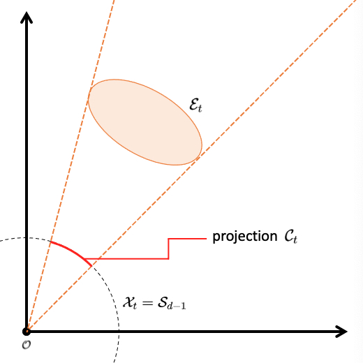
As is illustrated in Figure 1. The set of potentially optimal actions $\mathcal{C}_{t}$ is the projection of the confidence ellipsoid $\mathcal{E}_{t}$ onto ${\mathcal{S}}_{d-1}$. It’s hard to get a closed-form expression for $\mathcal{C}_{t}$, so we cannot directly calculate the range of $V_{t}^{-1}$-norm of actions in $\mathcal{C}_{t}$. Nevertheless, we can approximate the range by investigating the geometric properties of the ellipsoids.

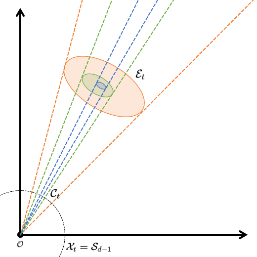
The intuition here is that, when POFUL has implemented sufficient exploration so that $\mathcal{E}_{t}$ is small enough, $\mathcal{C}_{t}$ concentrates accordingly to a small cap on ${\mathcal{S}}_{d-1}$. All actions within $\mathcal{C}_{t}$ point to similar directions and thus have similar $V_{t}$-norm. (Note that for a unit vector $x$, we have that $\|x\|_{V_{t}}$ can be written as a weighted summation of the eigenvalues of $V_{t}$, where the weights are determined by the direction of $x$.) Hence we can bound the range of $V_{t}$-norm by investigating the concentration of $\mathcal{C}_{t}$, which is pure geometry, and we’ll use the range of $V_{t}$-norm to determine the range of $V_{t}^{-1}$-norm.

(a)

(b)

Figure 1: Illustration of the set $\mathcal{C}_{t}$ of potentially optimal actions in $\mathbb{R}^{2}$. (a): $\mathcal{C}_{t}$ is the projection of $\mathcal{E}_{t}$ onto ${\mathcal{S}}_{d-1}$. (b): As the decision-maker collects more and more data, the confidence ellipsoid $\mathcal{E}_{t}$ shrinks accordingly (here different color corresponds to different levels of exploration). The potentially optimal actions point to similar directions, which essentially determine their $V_{t}$-norm. Hence it’s plausible one could get a proper range of their $V_{t}$-norm using geometry.

The following main theorem of this paper derives an upper bound of $\alpha_{t}$ based on this idea. We sketch the proof in Section 5.3.

Theorem 2

Suppose $\mathcal{X}_{t}={\mathcal{S}}_{d-1}$ for all $t\in[T]$. Define $\beta^{PVT}_{t}\coloneqq\iota_{t}\beta^{RLS}_{t}$ and

$$\Phi_{t} =\begin{cases}(\lambda_{1}^{-1}+\lambda_{d}^{-1}-m_{t}\lambda_{1}^{-1}\lambda_{d}^{-1})^{\frac{1}{2}},&\ \ \ \ \textit{if}\ \|\widehat{\theta}_{t}\|_{V_{t}}\geq\beta^{RLS}_{t}\\ \lambda_{d}^{-\frac{1}{2}}(V_{t}),&\ \ \ \ \textit{if}\ \|\widehat{\theta}_{t}\|_{V_{t}}<\beta^{RLS}_{t}\end{cases},$$

$$\Psi_{t} =\begin{cases}(\lambda_{k}^{-1}+\lambda_{k+1}^{-1}-M_{t}\lambda_{k}^{-1}\lambda_{k+1}^{-1})^{\frac{1}{2}},&\textit{if}\ \|\widehat{\theta}_{t}\|_{V_{t}}\geq\beta^{PVT}_{t}\\ \lambda_{1}^{-\frac{1}{2}}(V_{t}),&\textit{if}\ \|\widehat{\theta}_{t}\|_{V_{t}}<\beta^{PVT}_{t}\end{cases},$$

where we let

$$\quad m_{t}=(\|\widehat{\theta}_{t}\|_{V_{t}}^{2}-(\beta^{RLS}_{t})^{2})/(\|\widehat{\theta}_{t}\|+\beta^{RLS}_{t}/\lambda_{d}(V_{t}))^{2},\quad M_{t}=\|\widehat{\theta}_{t}\|_{V_{t}^{2}}^{2}/(\|\widehat{\theta}_{t}\|_{V_{t}}^{2}-(\beta^{PVT}_{t})^{2})$$

and $k\in[d]$ is such that $\lambda_{k}(V)\leq M_{t}\leq\lambda_{k+1}(V)$. Then for all $t\in[T]$, conditioned on event $\widehat{\mathcal{A}}_{t}\cap\widetilde{\mathcal{A}}_{t}$, it holds for all $s\leq t$ that

$$\inf_{\theta\in\mathcal{E}_{t}^{PVT}}\|x^{\star}_{s}(\theta)\|_{V_{s}^{-1}}\geq\Psi_{s},\quad\sup_{\theta\in\mathcal{E}_{s}^{RLS}}\|x^{\star}_{s}(\theta)\|_{V_{s}^{-1}}\leq\Phi_{s},\quad\alpha_{s}\leq\widehat{\alpha}_{s}\coloneqq\Phi_{s}/\Psi_{s}.$$

To better understand what Theorem 2 implies, we discuss some special cases.

Case 1: a pure exploration regime.

When the decision-maker doesn’t care about the regret and adopts a pure exploration algorithm that plays actions in all directions sequentially, we expect $\lambda_{i}(V_{t})=\mathcal{O}(t)$ for all $i=1,\dots,d$. Then $\widehat{\alpha}_{t}\leq C$ for some constant $C>0$. Specifically, if $V_{t}=D\mathbb{I}_{d}$ for some constant $D>0$, we have $\|x\|_{V_{t}^{-1}}=D^{-1}\|x\|=D^{-1}$ for all $x\in{\mathcal{S}}_{d-1}$ and hence $\widehat{\alpha}_{t}=1$ .

Case 2: linear structures.

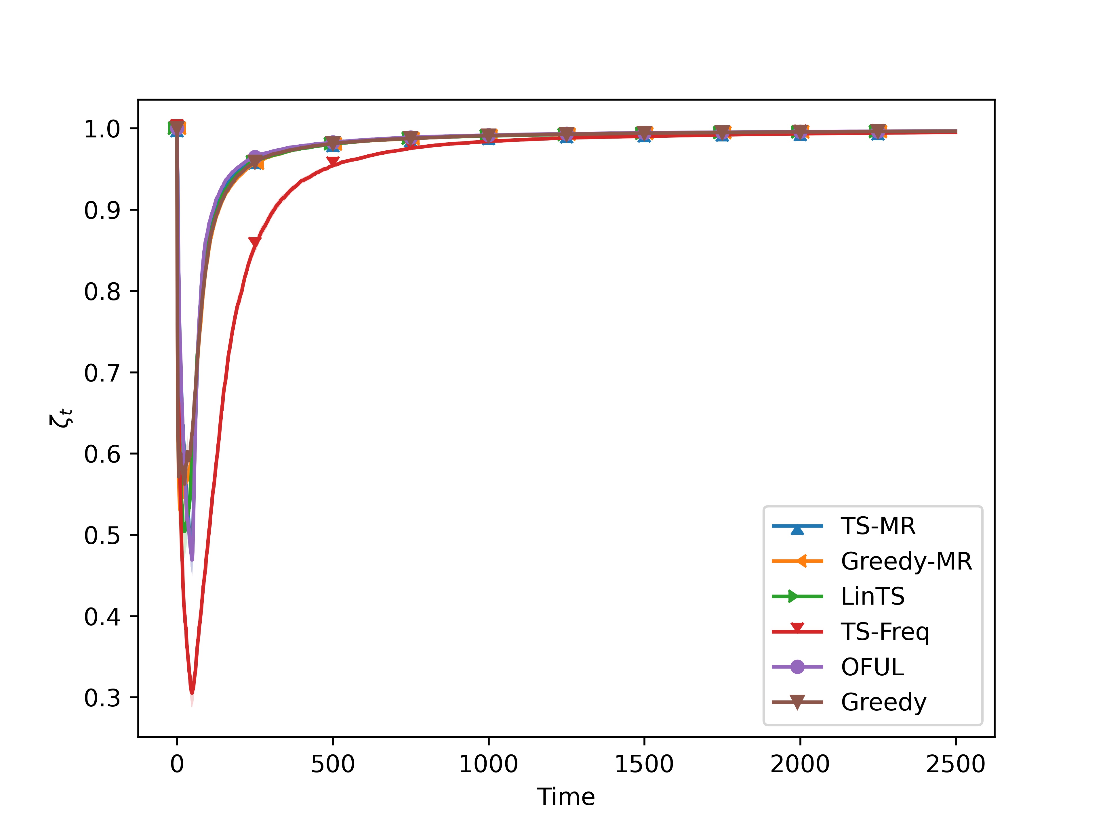
When the reward takes a linear form in the action, for example, the stochastic linear bandits we study, it’s observed in practice that the estimate $\widehat{\theta}_{t}$ tends to align in the first eigenspace of the uncertainty structure $V_{t}$ (empirically validated in Appendix 11). To see this, note that in order to maximize the reward in an online manner, bandit algorithms tend to select actions towards the confidence ellipsoid centered at $\widehat{\theta}_{t}$, hence forcing more exploration along the direction of $\widehat{\theta}_{t}$, especially at the late stage of the algorithm when the ellipsoid is small. The following proposition states that, as long as the center $\widehat{\theta}_{t}$ of the confidence ellipsoid $\mathcal{E}_{t}$ tends to be aligned with the first eigenspace of $V_{t}$, the corresponding uncertainty ratio tends to 1, indicating a regret bound matching the minimax $\widetilde{\mathcal{O}}(d\sqrt{T})$ rate by Theorem 1. This provides a plausible explanation for the empirical success of LinTS and Greedy.

Proposition 5

Suppose $\lim_{t\to\infty}\frac{\|\widehat{\theta}_{t}\|_{V_{t}}^{2}}{\|\widehat{\theta}_{t}\|^{2}}=\lambda_{\max}(V_{t})$, it holds that $\lim_{t\to\infty}\widehat{\alpha}_{t}=1$.

Remark 3

Clearly, one can further improve the bound in Equation (6) by plugging in the selected action $\widetilde{x}_{t}$. This is true for standard algorithms such as OFUL, LinTS, and Greedy. Explicitly, the uncertainty ratio can be bounded using $\widetilde{x}_{t}$ and Theorem 2 as

$$\alpha_{t}\leq\frac{\sup_{\theta\in\mathcal{E}_{t}^{RLS}}\|x^{\star}_{t}(\theta)\|_{V_{t}^{-1}}}{\|\widetilde{x}_{t}\|_{V_{t}^{-1}}}\leq\frac{\Phi_{t}}{\|\widetilde{x}_{t}\|_{V_{t}^{-1}}}.$$ (7)

However, for the variants of POFUL that we are going to propose in the Section 6, it is necessary to calculate the bound before selecting the action $\widetilde{x}_{t}$. Therefore, the bound shouldn’t depend on $\widetilde{x}_{t}$.

5.3 Sketch of the Proof

In this section, we present the proof of Theorem 2. In the remaining part of this section, we use a general confidence ellipsoid $\mathcal{E}_{t}(\delta)\coloneqq\left\{\theta\in\mathbb{R}^{d}:\|\theta-\widehat{\theta}_{t}\|_{V_{t}}\leq\beta_{t}(\delta)\right\}$ to represent $\mathcal{E}^{RLS}_{t}$ and $\mathcal{E}^{PVT}_{t}$, since the proof works for both of them.

First note that, when $\|\widehat{\theta}_{t}\|_{V_{t}}<\beta_{t}$, the bound in Theorem 2 becomes

$$\alpha_{t}\leq\lambda_{d}^{-\frac{1}{2}}(V_{t})/\lambda_{1}^{-\frac{1}{2}}(V_{t})=\sqrt{\lambda_{1}(V_{t})/\lambda_{d}(V_{t})}.$$

This bound holds trivially using the fact that $\lambda_{1}(V_{t})\leq\|x\|^{2}_{V_{t}}\leq\lambda_{d}(V_{t})$. This is the case when the data is insufficient and the confidence interval is too large to get a non-trivial upper bound for $\alpha_{t}$.

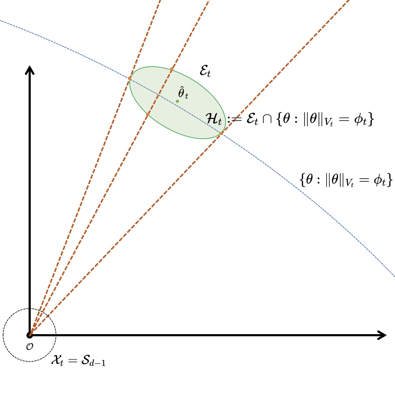
In the following, without loss of generality we assume $\|\widehat{\theta}_{t}\|_{V_{t}}^{2}\geq\beta_{t}^{2}$. The proof decomposes into three steps. In the first two steps, as is illustrated in $\mathbb{R}^{2}$ in Figure 2, we cut out a special hypersurface $\mathcal{H}_{t}$ within $\mathcal{E}_{t}$ and show that for all $\theta\in\mathcal{H}_{t}$, the corresponding optimal action $x^{\star}(\theta)$ has $V_{t}$-norm bounded from above and below. Note that the set of optimal actions for $\theta\in\mathcal{H}_{t}$ coincides with that for $\theta\in\mathcal{E}_{t}$, we get upper and lower bounds for $V_{t}$-norm of all potential actions in the ellipsoid. Next, we show that upper and lower bounds for the $V_{t}$-norm can be converted into upper and lower bounds for the $V_{t}^{-1}$-norm by solving a linear programming problem. Hence, we get an upper bound for $\alpha_{t}$ by calculating the ratio of the upper bound to the lower bound. We sketch the proof below and postpone the detailed proof for all lemmas in this section to Appendix 9.

Figure 2: Illustration of Step 1 and 2 in $\mathbb{R}^{2}$. Orange dashed rays: rays starting from the origin might have different numbers of intersections with $\mathcal{E}_{t}$, indicating whether the corresponding action lies in the projection of $\mathcal{E}_{t}$ onto ${\mathcal{S}}_{d-1}$. Blue dashed curve: the ellipsoid with fixed $V_{t}$-norm $\left\{\theta:\|\theta\|_{V_{t}}=\phi_{t}\right\}$. The intersection of this ellipsoid and $\mathcal{E}_{t}$ has the same projection as $\mathcal{E}_{t}$ onto ${\mathcal{S}}_{d-1}$.

In the following, we let $\phi_{t}\coloneqq\sqrt{\|\widehat{\theta}_{t}\|_{V_{t}}^{2}-\beta_{t}^{2}}$, which is well-defined since we assume $\|\widehat{\theta}_{t}\|_{V_{t}}\geq\beta_{t}$. In geometry, one can show that for a ray starting from the origin and intersecting $\mathcal{E}_{t}$ only at one point, $\phi_{t}$ is the ${V_{t}}$-norm of the intersection point.

Step 1. Upper Bounding the $V_{t}$-norm of actions.

Our first lemma investigates such intersection and provides an upper bound for the $V_{t}$-norm for the optimal actions corresponding to any $\theta\in\mathcal{E}_{t}$. The proof is based on investigating the condition for a ray paralleling an action $x\in{\mathcal{S}}_{d-1}$ to intersect with $\mathcal{E}_{t}$, which means $x$ is in the projection of $\mathcal{E}_{t}$ onto ${\mathcal{S}}_{d-1}$ and might become the optimal action $x^{\star}(\theta)$.

Lemma 1

For any $\theta\in\mathcal{E}_{t}$, we have $\|x^{\star}(\theta)\|_{V_{t}}\leq\|\widehat{\theta}_{t}\|_{V_{t}^{2}}/\phi_{t}$.

Step 2. Lower Bounding the $V_{t}$-norm of actions.

In order to lower bound the $V_{t}$-norm, we define the hypersurface $\mathcal{H}_{t}\coloneqq\mathcal{E}_{t}\cap\left\{\theta:\|\theta\|_{V_{t}}=\phi_{t}\right\}$, i.e., the intersection of the interior of the confidence ellipsoid $\mathcal{E}_{t}$ and the ellipsoid $\left\{\theta:\|\theta\|_{V_{t}}=\phi_{t}\right\}$. $\mathcal{H}_{t}$ consists of $\theta\in\mathcal{E}_{t}$ whose $V_{t}$-norm is $\phi_{t}$. One can check $\mathcal{H}_{t}$ is non-empty since $\phi_{t}\widehat{\theta}_{t}/\|\widehat{\theta}_{t}\|_{V_{t}}\in\mathcal{E}_{t}$, and the projection of $\mathcal{H}_{t}$ onto ${\mathcal{S}}_{d-1}$ is the same as that of $\mathcal{E}_{t}$ by convexity. Hence, it suffices to only consider $\theta\in\mathcal{H}_{t}$ as the corresponding set of optimal actions coincides. A lower bound for the $V_{t}$-norm is given by the following lemma.

Lemma 2

For any $\theta\in\mathcal{E}_{t}$, we have

$$\|x^{\star}(\theta)\|_{V_{t}}\geq\frac{\phi_{t}}{\|\widehat{\theta}_{t}\|+\beta_{t}/\lambda_{d}(V_{t})}.$$

The proof is directly using the fact that for any $\theta\in\mathcal{H}_{t}$, we have $\|\theta\|\leq\|\widehat{\theta}_{t}\|+\beta_{t}/\lambda_{d}(V_{t})$ and $\|\theta\|_{V_{t}}=\phi_{t}$. Also recall $x^{\star}(\theta)=\theta/\|\theta\|$ and hence $\|x^{\star}(\theta)\|_{V_{t}}=\|\theta\|_{V_{t}}/\|\theta\|$.

Step 3. Bounding the $V_{t}^{-1}$-norm of actions

The following lemma determines the range of action $x$’s $V_{t}^{-1}$-norm based on its $V_{t}$-norm range. It turns out that the two ranges can be related using the spectral information of the sample covariance matrix $V_{t}$, which is related to the shape of the confidence ellipsoid.

Lemma 3

Let $\{\lambda_{1},\lambda_{2},\dots,\lambda_{N_{V}}\}$ be the set of distinct eigenvalues of $V$ such that $\lambda_{1}>\lambda_{2}>\dots>\lambda_{N_{V}}>0$. Let $x\in\mathcal{B}_{d}$ satisfies $0<m\leq\|x\|_{V}^{2}\leq M$. We have

$$\frac{1}{\lambda_{k}}+\frac{1}{\lambda_{k+1}}-\frac{M}{\lambda_{k}\lambda_{k+1}}\leq\|x\|_{V^{-1}}^{2}\leq\frac{1}{\lambda_{1}}+\frac{1}{\lambda_{d}}-\frac{m}{\lambda_{1}\lambda_{d}},$$ (8)

where $k$ is such that $\lambda_{k}=\max_{i\in[N_{v}]}\{\lambda_{i}\geq M\}$.

The proof involves expressing the $V$- and $V^{-1}$-norms as weighted sums of $V$’s eigenvalues, then solving a linear programming (LP) problem constrained by the norm ranges.

By inserting the upper and lower bounds of the $V_{t}$-norm from Lemmas 1 and 2 into Lemma 3, we finalize the proof of Theorem 2.

6 A Meta-Algorithm for Course-Correction

In this section, we show how the data-driven regret bound can be utilized to improve standard bandit algorithms. Specifically, we propose a meta-algorithm that constructs course-corrected variants of the base algorithms. This ensures they achieve a minimax-optimal frequentist regret guarantee (up to constant factors) while retaining the majority of the original characteristics of the base algorithms, such as computational efficiency and low regret in most cases.

We take LinTS as an example and propose the algorithm Linear Thompson Sampling with Maximum Regret (Proxy) (TS-MR). The idea is to measure the performance of LinTS using $\widehat{\mu}_{t}$ and avoid bad LinTS actions by switching to OFUL actions when necessary.

Specifically, at each time $t$, TS-MR calculates the upper bound $\widehat{\mu}_{t}$ and compares it with a preset threshold $\mu$. If $\widehat{\mu}_{t}>\mu$, LinTS might be problematic and TS-MR takes an OFUL action to ensure a low instantaneous regret; if $\widehat{\mu}_{t}\leq\mu$, TS-MR takes the LinTS action. We remark that setting $\iota_{t}\equiv 0$ yields the corresponding Greedy-MR algorithm. The pseudocode is presented in Algorithm 2.

Algorithm 2 TS-MR (Greedy-MR)

0:  $T$, $\delta$, $\{\iota_{t}\}_{t\in[T]}$, $\mu$

  Initialize $V_{0}\leftarrow\lambda\mathbb{I}$, $\widehat{\theta}_{1}\leftarrow 0$, $\delta^{\prime}\leftarrow\delta/2T$

  for t = 1, 2 , …, T  do

     Calculate $\widehat{\alpha}_{t}$ using Theorem 2

     $\widehat{\mu_{t}}\leftarrow\widehat{\alpha}_{t}(1+\iota_{t})+1+\iota_{t}$

     if $\widehat{\mu}_{t}\leq\mu$ then

        Sample $\eta_{t}\sim\mathcal{D}^{SA}(\delta^{\prime})$ (defined in Section 3)

        $\widetilde{\theta}_{t}\leftarrow\widehat{\theta}_{t}+\iota_{t}\beta_{t}^{RLS}(\delta^{\prime})V_{t}^{-\frac{1}{2}}\eta_{t}$

        ${x}_{t}\leftarrow\arg\max_{x\in\mathcal{X}_{t}}\langle{x},{\widetilde{\theta}_{t}}\rangle$

     else

        ${x}_{t}\leftarrow\arg\max_{x\in\mathcal{X}_{t}}\arg\max_{\theta\in\mathcal{E}_{t}^{RLS}(\delta^{\prime})}\langle{x},{\widetilde{\theta}_{t}}\rangle$

     end if

     Observe reward $r_{t}$

     $V_{t+1}\leftarrow V_{t}+{x}_{t}{x}_{t}^{\top}$

     $\widehat{\theta}_{t+1}\leftarrow V_{t+1}^{-1}\sum_{s=1}^{t}x_{s}r_{s}$.

  end for

By construction, the course-corrected algorithms have $\mu_{t}\leq\max\{\mu,2\}$ for all $t\in[T]$. Using Theorem 1, we get the following frequentist regret for them, which is optimal up to a constant factor.

Corollary 1

TS-MR and Greedy-MR achieve a frequentist regret of $\mathcal{R}(T)=\widetilde{\mathcal{O}}\left(\max\{\mu,2\}d\sqrt{T}\right)$.

Remark 4

In practice, the choice of the threshold $\mu$ depends on the problem settings. In a high-risk setting where LinTS and Greedy fail with high probability, one can set a small $\mu$ so that TS-MR and Greedy-MR select more OFUL actions to guarantee the necessary amount of exploration. In a low-risk setting where original LinTS and Greedy algorithms work well, one can set a large $\mu$ and hence TS-MR and Greedy-MR select TS and greedy actions respectively to avoid unnecessary exploration and save the computational cost.

7 Simulations

In this section, we present the simulation results of TS-MR, Greedy-MR, and other baseline algorithms.

7.1 Synthetic datasets

(a) example 1

(b) example 2

(c) example 3

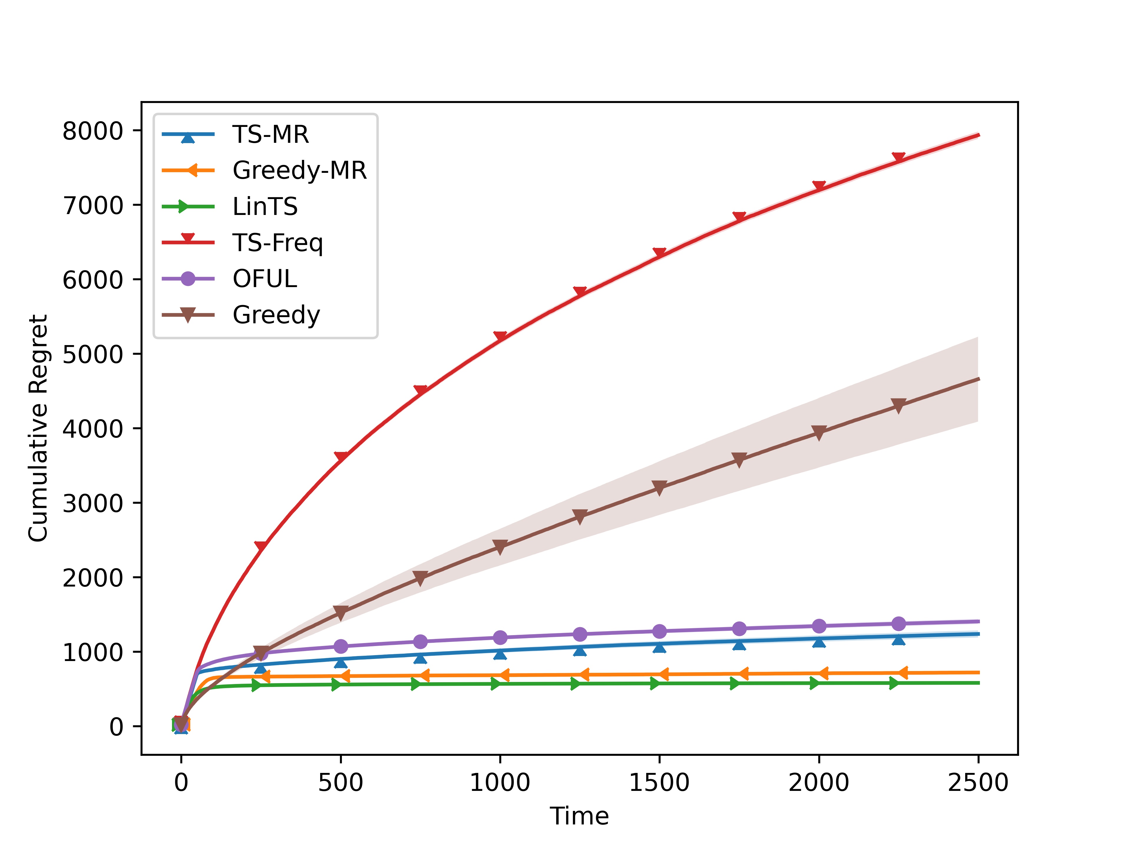
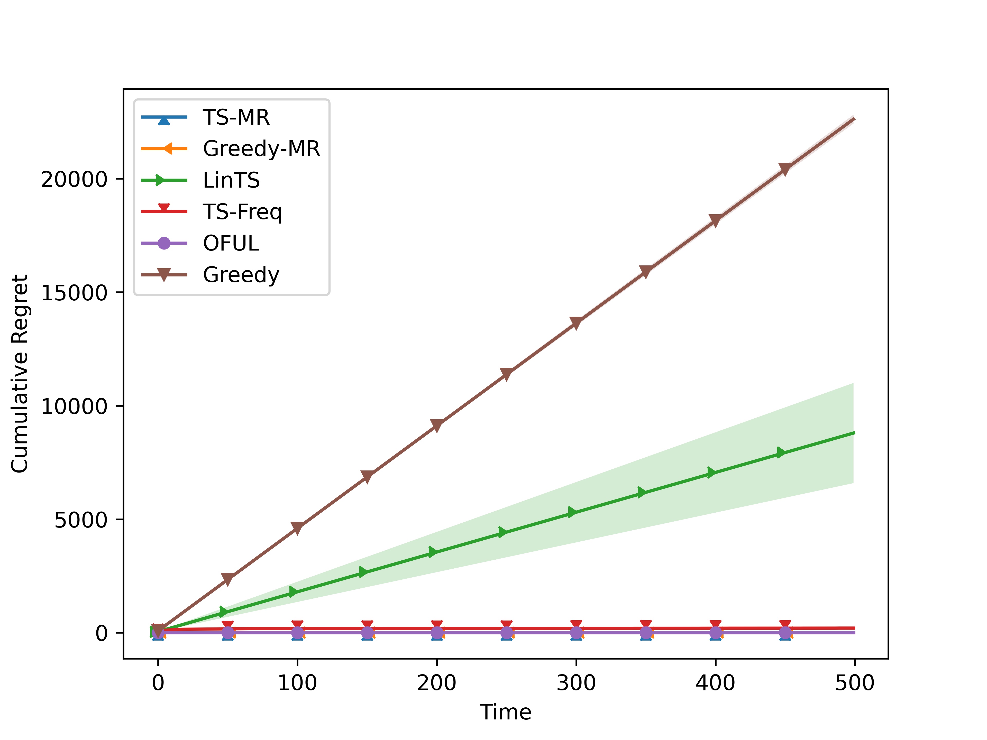
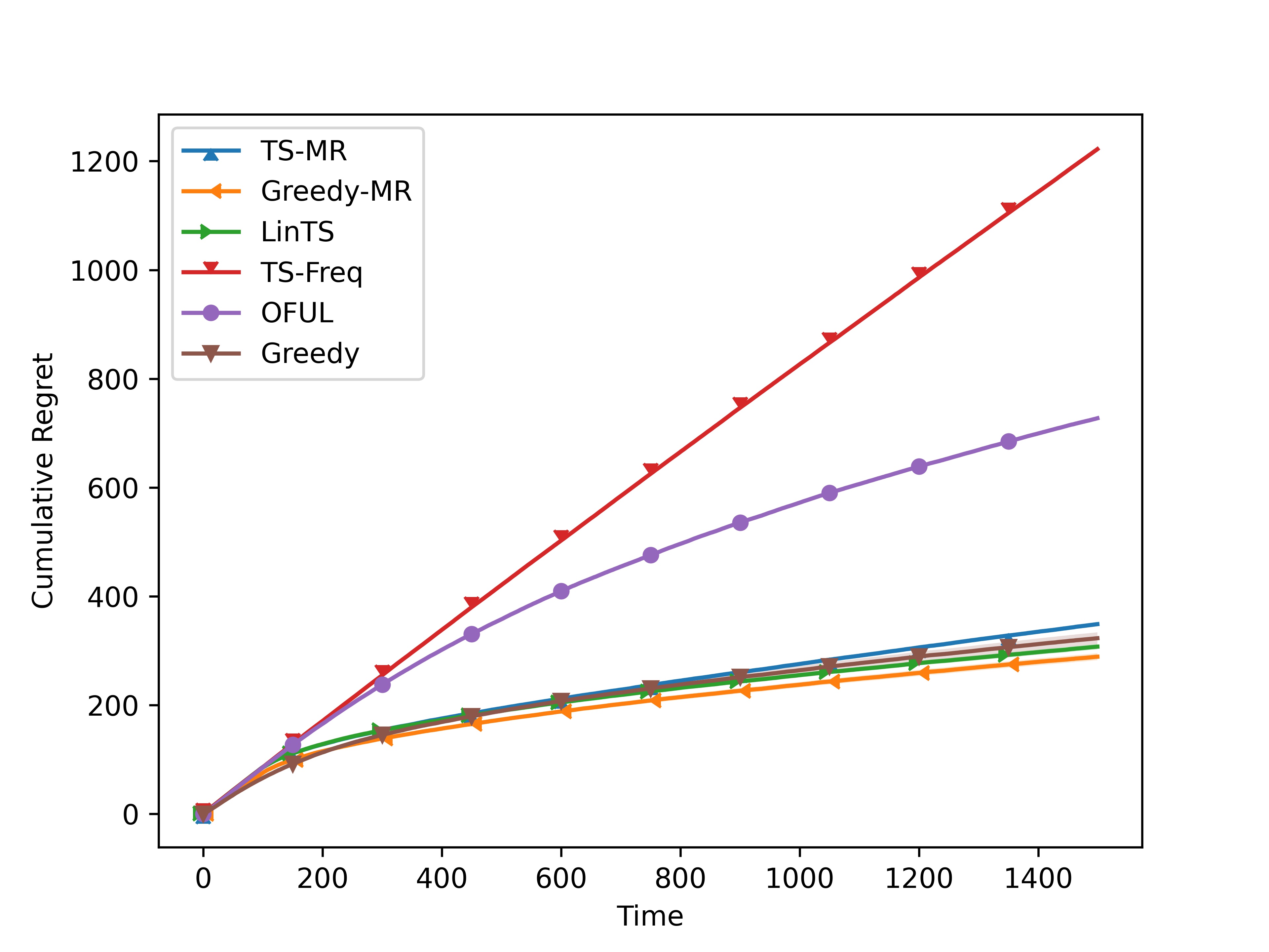
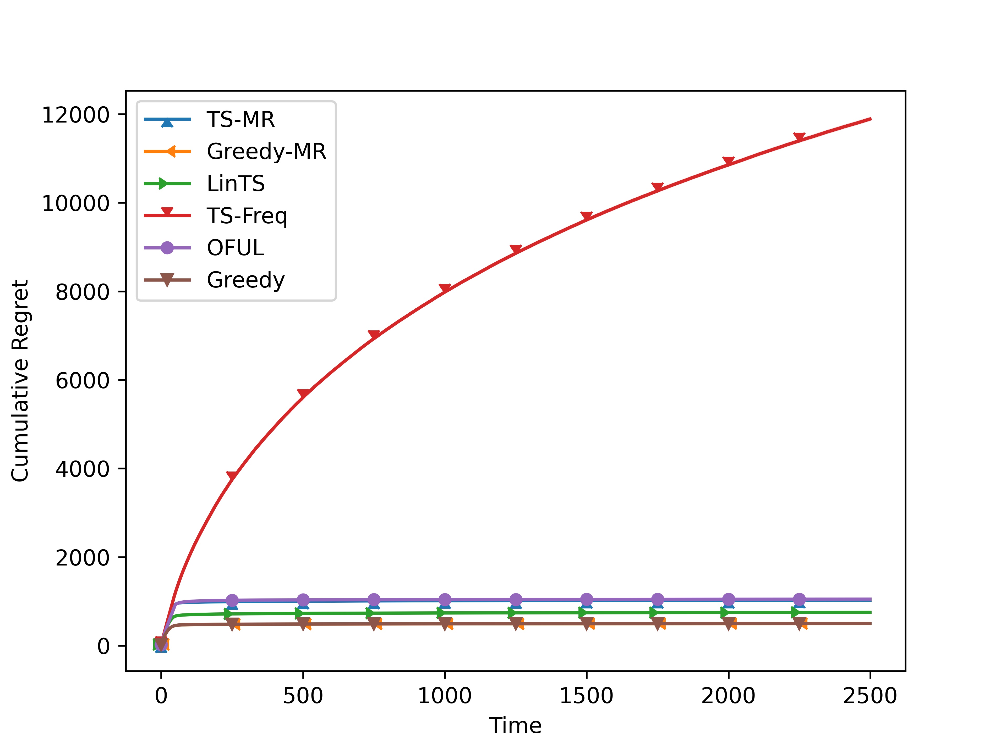
Figure 3: Comparison of the cumulative regret incurred by TS-MR and Greedy-MR, versus the baseline algorithms in Examples 1-3.

Example 1. Stochastic linear bandit with uniformly and independently distributed actions.

We fix $d=50$, and sample $\theta^{\star}\sim\text{Unif}(\{\theta\in\mathbb{R}^{d}|\|\theta\|=10\})$ on a sphere with fixed norm. At each time $t$, we generate 100 i.i.d. random actions sampled from $\text{Unif}({\mathcal{S}}_{d-1})$ to form $\mathcal{X}_{t}$. This is a basic example of standard stochastic linear bandit problems without any extra structure. We set the threshold $\mu=8$ for TS-MR and Greedy-MR. We average simulation results over 100 independent runs. The results are summarized in Figure 3(a). TS-Freq shows pessimistic regret due to the inflation of the posterior, while other algorithms in general perform well.

Example 2. Contextual bandits embedded in the linear bandit problem (Abbasi-Yadkori, 2013).

We fix $d=50$, and sample $\theta^{\star}\sim\text{Unif}(\{\theta\in\mathbb{R}^{d}|\|\theta\|=70\})$. At each time $t$, we first generate a random vector $u_{t}\sim\mathcal{N}(0,\mathbb{I}_{5})$ and let $x_{t,i}\in\mathbb{R}^{50}$ be the vector whose $i$-th block of size 5 is a copy of $u_{t}$, and other components are 0. Then $X_{t}=\{x_{t,i}\}_{i\in[10]}$ is an action set of size 10, sharing the same feature $u_{t}$ in different blocks. This problem is equivalent to a 10-armed contextual bandit. We ser $\mu=12$ for TS-MR and Greedy-MR. Again, we average simulation results over 100 independent runs. The results are summarized in Figure 3(b). In this setting, Greedy performs suboptimally due to a lack of exploration for some arms. Nevertheless, Greedy-MR outperforms both Greedy and OFUL by adaptively choosing OFUL actions only when it detects large regret proxy $\widehat{\mu}_{t}$.

Example 3. Prior mean mismatch (Hamidi and Bayati, 2020b).

This is an example in which LinTS is shown to incur linear Bayesian regret. We sample $\theta^{\star}\sim\mathcal{N}(m\mathbf{1}_{3d},\mathbb{I}_{3d})$ and fix the action set $\mathcal{X}_{t}=\{0,x_{a},x_{b}\}$ for all $t\in[T]$, where $x_{a}=-\sum_{i=1}^{d}\frac{e_{i}}{\sqrt{3d}},\quad x_{b}=\sum_{i=11}^{3d}\frac{e_{i}}{\sqrt{3d}}-\sum_{i=1}^{d}\frac{e_{i}}{\sqrt{3d}}$. It is shown in Hamidi and Bayati (2020b) that, when LinTS takes a wrong prior mean as input, it has a large probability to choose $\widetilde{x}_{2}=0$, conditioned on $\widetilde{x}_{1}=x_{a}$. Note that choosing the zero action brings no information update to LinTS, it suffers a linear Bayesian regret when trying to escape from the zero action. We let $m=10$ and set $d=10$, so the problem is a $30$-dimensional linear bandit. We ser $\mu=12$ for TS-MR and Greedy-MR. We carried out 100 independent runs. The results are summarized in Figure 3(c). We see both LinTS and Greedy incur linear regrets as expected, while TS-MR and Greedy-MR, switch to OFUL adaptively to tackle this hard problem and achieve sublinear regret.

7.2 Real-world datasets

We explore the performance of standard POFUL algorithms and the proposed TS-MR and Greedy-MR algorithms on real-world datasets. We consider three datasets for classification tasks on the OpenML platform, Cardiotocography, JapaneseVowels and Segment. They focus on healthcare, pattern recognition, and computer vision problems respectively.

Setup.

We follow the standard approach in the literature that converts classification tasks to contextual bandit problems, and then embeds it into linear bandit problems in the same way as Example 2 in Section 6. Specifically, we regard each class as an action so that at each time, the decision-maker assigns a class to the feature observed and receives a binary reward, namely 1 for assigning the correct class and 0 otherwise, plus a Gaussian noise.

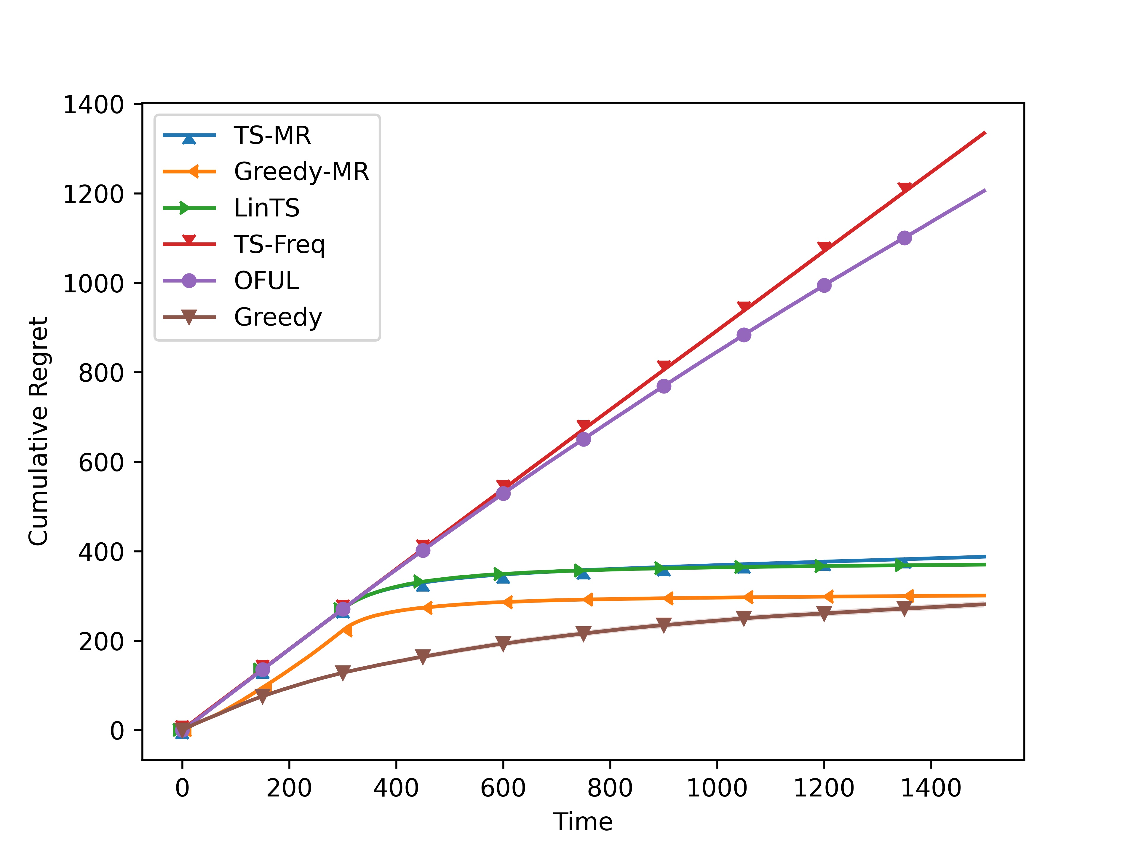
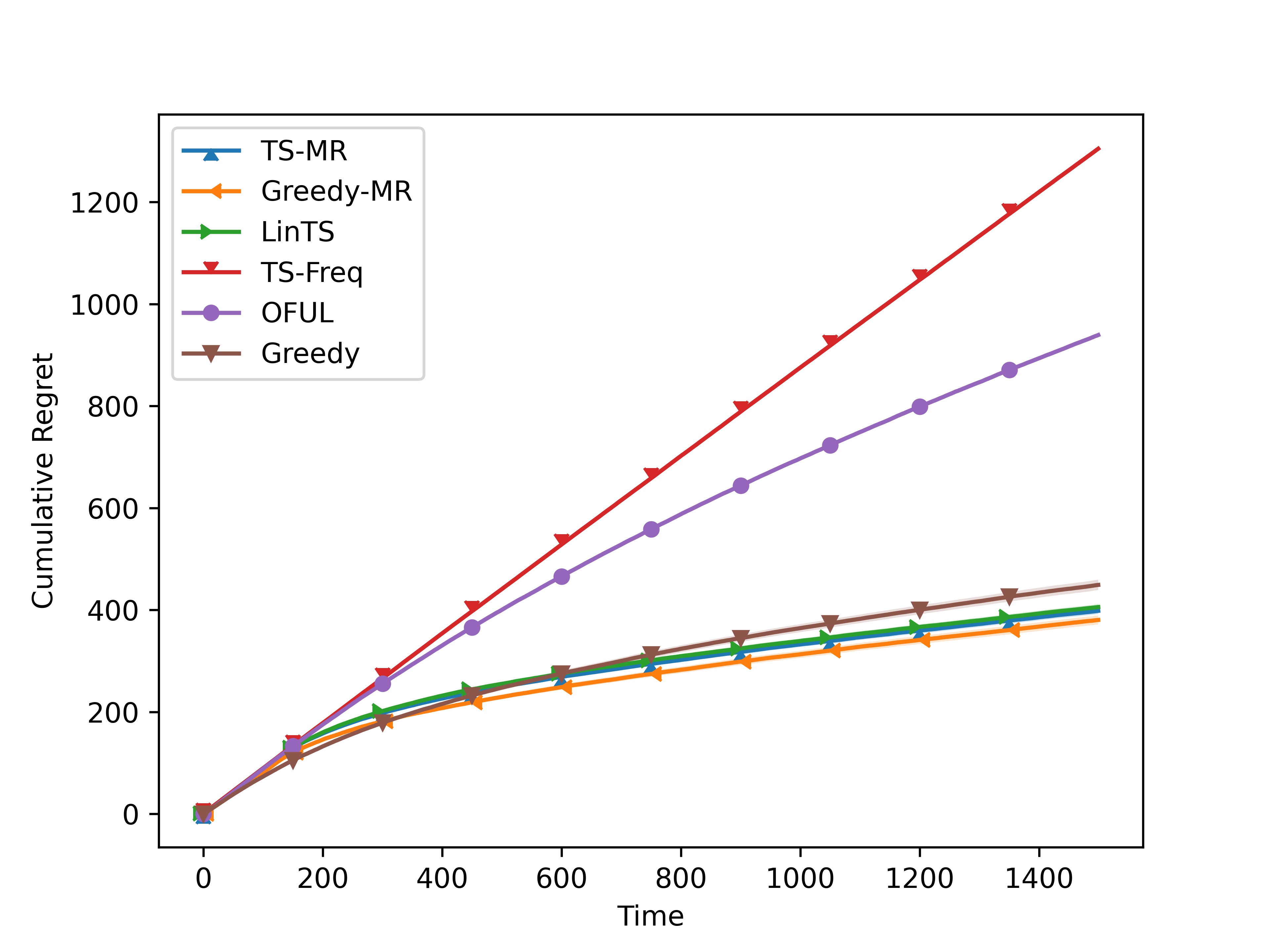
We plot the cumulative regret (averaged over 100 duplicates) for all algorithms. Figure 4 shows that for all real-world datasets: OFUL and TS-Freq perform poorly due to their conservative exploration; LinTS and Greedy are achieving empirical success even though they don’t have theoretical guarantees; TS-MR and Greedy-MR retain the desirable empirical performance of LinTS and Greedy, while enjoying the minimax optimal frequentist regret bound.

(a) Cardiotocography dataset.

(b) JapaneseVowels dataset.

(c) Segment dataset.

Figure 4: Cumulative regret of all algorithms on real-world datasets.

8 Conclusion

In this work, we propose a data-driven framework to analyze the frequentist regret of POFUL, a family of algorithms that includes OFUL, LinTS, TS-Freq, and Greedy as special cases. Our approach allows for the computation of an instance-dependent frequentist regret bound for POFUL during implementation, which subsequently informs the course-correction of the algorithm. Our technique conducts a novel real-time geometric analysis of the $d$-dimensional confidence ellipsoid to fully leverage the historical information and might be of independent interest. As applications, we propose TS-MR and Greedy-MR algorithms that enjoy provable minimax optimal frequentist regret and demonstrate their ability to adaptively switch to OFUL when necessary in hard problems where LinTS and Greedy fail. We hope this work provides a steady step towards bridging the gap between theoretical guarantees and empirical performance of bandit algorithms such as LinTS and Greedy.

9 Proof of Lemmas for Theorem 2

9.1 Proof of Lemma 1

Proof.

Let $\theta=tx$ where $x$ is any unit vector in $\mathbb{R}^{d}$ and $t\in\mathbb{R}^{+}$ is a scalar. Consider the equation that characterizes the intersection $\{tx:t\in\mathbb{R}^{+}\}\cap\mathcal{E}_{t}$, namely $(tx-\widehat{\theta}_{t})^{\top}V_{t}(tx-\widehat{\theta}_{t})\leq\beta_{t}^{2}$. Equivalently, we have $t^{2}\|x\|_{V_{t}}^{2}-2tx^{\top}V_{t}\widehat{\theta}_{t}+\phi_{t}^{2}\leq 0$. This quadratic inequality of $t$ has at least one solution if the discriminant is non-negative, i.e. $4(x^{\top}V_{t}\widehat{\theta})^{2}\geq 4\|x\|_{V_{t}}^{2}\phi_{t}^{2}$. Then by direct computation,

$$\|x\|_{V_{t}}\leq\frac{\sqrt{(x^{\top}V_{t}\widehat{\theta}_{t})^{2}}}{\phi_{t}}\leq\frac{\sqrt{x^{\top}x}\sqrt{(\widehat{\theta}_{t})^{\top}V_{t}^{\top}V_{t}\widehat{\theta}_{t}}}{\phi_{t}}=\frac{\|\widehat{\theta}_{t}\|_{V_{t}^{2}}}{\phi_{t}}.$$

Note that $\theta\in\mathcal{E}_{t}$ if and only if $\theta$ is on a ray starting from the origin and intersects $\mathcal{E}_{t}$ at one or more points. Namely, $\theta=tx$ for some $x$ that satisfies $4(x^{\top}V_{t}\widehat{\theta})^{2}\geq 4\|x\|_{V_{t}}^{2}\phi_{t}^{2}$, we conclude the proof.

∎

9.2 Proof of Lemma 2

Proof.

Note that for any $\theta\in\mathcal{H}_{t}\subset\mathcal{E}_{t}$, it holds that $\|\theta\|\leq\|\widehat{\theta}_{t}\|+\beta_{t}/\lambda_{d}(V_{t})$. Also, by the construction of $\mathcal{H}_{t}$, we have $\|\theta\|_{V_{t}}=\phi_{t}$. Then by direct computation, we have

$$\|x^{\star}(\theta)\|_{V_{t}}=\frac{\|\theta\|_{V_{t}}}{\|\theta\|}\geq\frac{\phi_{t}}{\|\widehat{\theta}_{t}\|+\beta_{t}/\lambda_{d}(V_{t})}.$$

To prove the same result for any $\theta\in\mathcal{E}_{t}$, we only need to show there exists $\theta^{\prime}\in\mathcal{H}_{t}$ such that $x^{\star}(\theta)=x^{\star}(\theta^{\prime})$. To see this, let $x=\theta/\|\theta\|$ and consider the intersection $\{tx:t\in\mathbb{R}^{+}\}\cap\mathcal{E}_{t}$, which is non-empty by our choice of $\theta$. Similar to the proof of Lemma 1, the discriminant is non-negative, i.e. $4(x^{\top}V_{t}\widehat{\theta})^{2}\geq 4\|x\|_{V_{t}}^{2}\phi_{t}^{2}$.

Now consider the intersection $\{tx:t\in\mathbb{R}\}\cap\partial\mathcal{E}_{t}$, where we let $\partial\mathcal{E}_{t}\coloneqq\left\{\theta\in\mathbb{R}^{d}:\|\theta-\widehat{\theta}_{t}\|_{V_{t}}=\beta_{t}(\delta)\right\}$ be the border of the ellisoid. The intersection points are characterized by the solution to

$$t^{2}\|x\|_{V_{t}}^{2}-2tx^{\top}V_{t}\widehat{\theta}_{t}+\phi_{t}^{2}=0.$$ (9)

If $4(x^{\top}V_{t}\widehat{\theta})^{2}=4\|x\|_{V_{t}}^{2}\phi_{t}^{2}$ and there is only one intersection point, namely $\theta$ itself, we have

$$0=t^{2}\|x\|_{V_{t}}^{2}-2tx^{\top}V_{t}\widehat{\theta}_{t}+\phi_{t}^{2}=t^{2}\|x\|_{V_{t}}^{2}-2t\|x\|_{V_{t}}\phi_{t}+\phi_{t}^{2}=(\|tx\|_{V_{t}}-\phi_{t})^{2}.$$

Therefore, we have $\|\theta\|_{V_{t}}=\|tx\|_{V_{t}}=\phi_{t}$, i.e. $\theta\in\mathcal{H}_{t}$.

If $4(x^{\top}V_{t}\widehat{\theta})^{2}>4\|x\|_{V_{t}}^{2}\phi_{t}^{2}$, it follows that $x^{\top}V_{t}\widehat{\theta}>\|x\|_{V_{t}}\phi_{t}$. This inference is valid given that $x^{\top}V_{t}\widehat{\theta}>0$, which can be verified using Equation (9) and noting that $t>0$. Consider the solutions to (9)

$$t_{1}=\frac{x^{\top}V_{t}\widehat{\theta}_{t}-\sqrt{(x^{\top}V_{t}\widehat{\theta})^{2}-\|x\|_{V_{t}}^{2}\phi_{t}^{2}}}{\|x\|_{V_{t}}^{2}},\quad t_{2}=\frac{x^{\top}V_{t}\widehat{\theta}_{t}+\sqrt{(x^{\top}V_{t}\widehat{\theta})^{2}-\|x\|_{V_{t}}^{2}\phi_{t}^{2}}}{\|x\|_{V_{t}}^{2}}.$$

We only need to show $\|t_{1}x\|_{V_{t}}<\phi_{t}<\|t_{2}x\|_{V_{t}}$, then by the continuity of $\|\cdot\|_{V_{t}}$ and the convexity of $\mathcal{E}_{t}$, there exists $t^{\prime}\in(t_{1},t_{2})$ such that $\|t^{\prime}x\|_{V_{t}}=\phi_{t}$. Then $\theta^{\prime}\coloneqq t^{\prime}x\in\mathcal{H}_{t}$ is the desired point. By direct computation,

$$\|t_{1}x\|_{V_{t}}=\frac{x^{\top}V_{t}\widehat{\theta}_{t}-\sqrt{(x^{\top}V_{t}\widehat{\theta})^{2}-\|x\|_{V_{t}}^{2}\phi_{t}^{2}}}{\|x\|_{V_{t}}}.$$

We only need to prove

$$x^{\top}V_{t}\widehat{\theta}_{t}-\|x\|_{V_{t}}\phi_{t}\leq\sqrt{(x^{\top}V_{t}\widehat{\theta})^{2}-\|x\|_{V_{t}}^{2}\phi_{t}^{2}}$$

Note that

$$(x^{\top}V_{t}\widehat{\theta}_{t}-\|x\|_{V_{t}}\phi_{t})^{2} =(x^{\top}V_{t}\widehat{\theta})^{2}-2x^{\top}V_{t}\widehat{\theta}\phi_{t}\|x\|_{V_{t}}+\|x\|_{V_{t}}^{2}\phi_{t}^{2}$$

$$\leq(x^{\top}V_{t}\widehat{\theta})^{2}-2\|x\|_{V_{t}}^{2}\phi_{t}^{2}+\|x\|_{V_{t}}^{2}\phi_{t}^{2}$$

$$=(x^{\top}V_{t}\widehat{\theta})^{2}-\|x\|_{V_{t}}^{2}\phi_{t}^{2}$$

where we have used the fact that $x^{\top}V_{t}\widehat{\theta}>\|x\|_{V_{t}}\phi_{t}$ in the ineuqlity. Taking square root for both sides yields the desired result, and hence $\|t_{1}x\|_{V_{t}}<\phi_{t}$. Similarly, one can show $\phi_{t}<\|t_{2}x\|_{V_{t}}$. This concludes the proof.

∎

9.3 Proof of Lemma 3

Proof.

Let $\{\lambda_{1},\lambda_{2},\dots,\lambda_{N_{V}}\}$ be the set of distinct eigenvalues of $V$. By the spectral theorem, $V$ can be decomposed as $V=U\Lambda U^{\top}$, where the columns of $U$ consist of orthonormal eigenvectors of $V$, denoted by $\{u_{11},\dots,u_{1n_{1}},u_{21},\dots,u_{2n_{2}},\dots,u_{N_{V}1},\dots,u_{N_{V}n_{N_{V}}}\}$, where $n_{1},\dots,n_{N_{V}}$ are the algebraic multiplicity of the eigenvalues respectively. Since $V$ is a symmetric matrix, the eigenvectors for a basis of $\mathbb{R}^{d}$ and we have $\sum_{i=1}^{N_{V}}n_{i}=d$. We can write $x$ as a linear combination $x=\sum_{i=1}^{N_{V}}\sum_{j=1}^{n_{i}}w_{ij}u_{ij}$, where $\sum_{i=1}^{N_{V}}\sum_{j=1}^{n_{i}}w_{ij}^{2}=1$. Define $a_{i}\coloneqq\sum_{j=1}^{n_{i}}w_{ij}^{2}$, by direct computation, we have $\sum_{i=1}^{N_{V}}a_{i}=1$ and $\|x\|_{V}^{2}=\sum_{i=1}^{N_{V}}\lambda_{i}a_{i}$ and $\|x\|_{V^{-1}}^{2}=\sum_{i=1}^{N_{V}}\lambda_{i}^{-1}a_{i}$ .

Now we study the range of $\|x\|_{V^{-1}}^{2}$ when $\|x\|_{V}^{2}$ is bounded as $m\leq\|x\|_{V}^{2}\leq M$. First, let’s focus on maximizing $\|x\|_{V^{-1}}^{2}$, it suffices to solve the LP problem

maximize $$\sum_{i=1}^{N_{V}}a_{i}\lambda_{i}^{-1}\quad\text{s.t.}\quad\forall i,a_{i}\geq 0,\ \sum_{i=1}^{N_{V}}a_{i}=1,\ \sum_{i=1}^{N_{V}}a_{i}\lambda_{i}\geq m,\ \sum_{i=1}^{N_{V}}a_{i}\lambda_{i}\leq M.$$

The Lagrangian is given by

$$L=\sum_{i=1}^{N_{V}}a_{i}\lambda_{i}^{-1}+\mu(1-\sum_{i=1}^{N_{V}}a_{i})+\eta(\sum_{i=1}^{N_{V}}a_{i}\lambda_{i}-m)+\gamma(M-\sum_{i=1}^{N_{V}}a_{i}\lambda_{i})+\sum_{i=1}^{N_{V}}\kappa_{i}a_{i}.$$

The KKT conditions are given by

$$\begin{cases}&\nabla_{a_{i}}L=\lambda_{i}^{-1}-\mu+\eta\lambda_{i}-\gamma\lambda_{i}+\kappa_{i}=0,\\ &a_{i}\geq 0,\forall i,\sum_{i=1}^{N_{V}}a_{i}=1,\sum_{i=1}^{N_{V}}a_{i}\lambda_{i}\geq m,\sum_{i=1}^{N_{V}}a_{i}\lambda_{i}\leq M,\\ &\eta\geq 0,\gamma\geq 0,\kappa_{i}\geq 0,\forall i,\\ &\eta(\sum_{i=1}^{N_{V}}a_{i}\lambda_{i}-m)=0,\gamma(M-\sum_{i=1}^{N_{V}}a_{i}\lambda_{i})=0,\kappa_{i}a_{i}=0,\forall i.\end{cases}$$ (10)

To satisfy the first condition above, $\kappa_{i}$’s can only be zero for at most two indices. Hence, $a_{i}$ can only be non-zero for at most two distinct eigenvalues, denoted by $\lambda_{i}$ and $\lambda_{j}$, where $i<j$ and $\lambda_{i}>\lambda_{j}$. Namely, the solution to (LABEL:eq:KKT) lies in the subspace spanned by the eigenvectors corresponding to $\lambda_{i}$ and $\lambda_{j}$.

Let $y=\|x\|_{V}^{2}$, we have $a_{i}\lambda_{i}+a_{j}\lambda_{j}=y$ and $a_{i}\lambda_{i}^{-1}+a_{j}\lambda_{j}^{-1}=\|x\|_{V^{-1}}^{2}$. Note that $\sum_{i=1}^{N_{V}}a_{i}=a_{i}+a_{j}=1$, by direct computation, the closed form of $\|x\|_{V^{-1}}^{2}$ is given by $\|x\|_{V^{-1}}^{2}=\frac{1}{\lambda_{i}}+\frac{1}{\lambda_{j}}-\frac{y}{\lambda_{i}\lambda_{j}}\eqqcolon f(y,\lambda_{i},\lambda_{j})$.

Clearly, we have

$$\begin{cases}\frac{\partial f}{\partial y}&=-\frac{1}{\lambda_{i}\lambda_{j}}<0,\\ \frac{\partial f}{\partial\lambda_{i}}&=(\frac{y}{\lambda_{j}}-1)\frac{1}{\lambda_{i}^{2}}>0,\\ \frac{\partial f}{\partial\lambda_{j}}&=(\frac{y}{\lambda_{i}}-1)\frac{1}{\lambda_{j}^{2}}<0.\end{cases}$$

Then the maximum of $\|x\|_{V^{-1}}^{2}$ is obtained when $\lambda_{i}=\lambda_{1}$, $\lambda_{j}=\lambda_{N_{V}}$, $y=m$. Therefore, the solution to the LP problem is any unit vector $x^{\star}_{\max}$ that lies in the subspace spanned by the eigenvectors corresponding to $\lambda_{1}$ and $\lambda_{N_{V}}$. Moreover, we have

$$\|x^{\star}_{\max}\|_{V^{-1}}^{2}=\frac{1}{\lambda_{1}}+\frac{1}{\lambda_{N_{V}}}-\frac{m}{\lambda_{1}\lambda_{N_{V}}}.$$

Similarly, by investigating the KKT conditions for the LP problem that minimize $\sum_{i=1}^{N_{V}}a_{i}\lambda_{i}^{-1}$, the minimum of $\|x\|_{V^{-1}}^{2}$ is obtained when $\lambda_{i}=\lambda_{k}$, $\lambda_{j}=\lambda_{k+1}$, $y=M$, where $k$ is such that $\lambda_{k}=\max_{i\in[N_{v}]}\{\lambda_{i}\geq M\}$, and hence $\lambda_{k+1}=\min_{i\in[N_{v}]}\{\lambda_{i}<M\}$. The solution vector is any unit vector $x^{\star}_{\min}$ that lies in the subspace spanned by the eigenvectors corresponding to $\lambda_{k}$ and $\lambda_{k+1}$, and we have

$$\|x^{\star}_{\min}\|_{V^{-1}}^{2}=\frac{1}{\lambda_{k}}+\frac{1}{\lambda_{k+1}}-\frac{M}{\lambda_{k}\lambda_{k+1}}.$$

This concludes the proof.

∎

10 Other Proofs

10.1 Proof of Proposition 3

Proof.

By Propostion 1, we have

$${\mathbb{P}}\left[\widehat{\mathcal{A}}_{T}\right] ={\mathbb{P}}\left[\cap_{t=1}^{T}\left\{\|\widehat{\theta}_{t}-\theta^{\star}_{t}\|_{V_{t}}\leq\beta^{RLS}_{t}(\delta^{\prime})\right\}\right]$$

$$\geq 1-\sum_{t=1}^{T}{\mathbb{P}}\left[\|\widehat{\theta}_{t}-\theta^{\star}_{t}\|_{V_{t}}\leq\beta^{RLS}_{t}(\delta^{\prime})\right]$$

$$\geq 1-\frac{\delta}{2}.$$

Similarly, by Definition 2, we have

$${\mathbb{P}}\left[\widetilde{\mathcal{A}}_{T}\right] ={\mathbb{P}}\left[\cap_{t=1}^{T}\left\{\widetilde{\theta}_{t}\in\mathcal{E}_{t}^{PVT}(\delta^{\prime})|\mathcal{F}_{t}\right\}\right]$$

$$\geq 1-\sum_{t=1}^{T}{\mathbb{P}}\left[\widetilde{\theta}_{t}\in\mathcal{E}_{t}^{PVT}(\delta^{\prime})|\mathcal{F}_{t}\right]$$

$$\geq 1-\frac{\delta}{2}.$$

Combining the two inequalities above, we have ${\mathbb{P}}\left[\mathcal{A}_{T}\right]\geq 1-\delta$. ∎

10.2 Proof of Proposition 4

Proof.

Since ${\theta}^{\star}\in\mathcal{E}_{t}^{RLS}(\delta^{\prime})$ and $\widetilde{\theta}_{t}\in\mathcal{E}_{t}^{PVT}(\delta^{\prime})$, it holds that

$$\|{\theta}^{\star}-\widehat{\theta}_{t}\|_{V_{t}}\leq\beta_{t}^{RLS}(\delta^{\prime}),\quad\|\widetilde{\theta}_{t}-\widehat{\theta}_{t}\|_{V_{t}}\leq\beta^{PVT}_{t}(\delta^{\prime})=\iota_{t}\beta^{RLS}_{t}(\delta^{\prime}).$$ (11)

In the following, we drop the dependence on $\delta^{\prime}$ for notation simplicity. We have

$$\langle{x_{t}^{\star}},{\theta^{\star}}\rangle-\langle{\widetilde{x}_{t}},{\theta^{\star}}\rangle =\left(\langle{x^{\star}_{t}},{\theta^{\star}}\rangle-\langle{x^{\star}_{t}},{\widetilde{\theta}_{t}}\rangle\right)+\left(\langle{x^{\star}_{t}},{\widetilde{\theta}_{t}}\rangle-\langle{\widetilde{x}_{t}},{\widetilde{\theta}_{t}}\rangle\right)$$

$$\quad+\left(\langle{\widetilde{x}_{t}},{\widetilde{\theta}_{t}}\rangle-\langle{\widetilde{x}_{t}},{\widehat{\theta}_{t}}\rangle\right)+\left(\langle{\widetilde{x}_{t}},{\widehat{\theta}_{t}}\rangle-\langle{\widetilde{x}_{t}},{\theta^{\star}}\rangle\right).$$

To bound the second term on the right hand side, recall by Equation (3) the POFUL action $\widetilde{x}_{t}$ satisfies

$$\langle{x^{\star}_{t}},{\widetilde{\theta}_{t}}\rangle+\tau_{t}\|x^{\star}_{t}\|_{V^{-1}_{t}}\beta_{t}^{RLS}\leq\langle{\widetilde{x}_{t}},{\widetilde{\theta}_{t}}\rangle+\tau_{t}\|\widetilde{x}_{t}\|_{V^{-1}_{t}}\beta_{t}^{RLS}.$$

Rearranging the ineuqlity, we obtain $\langle{x^{\star}_{t}},{\widetilde{\theta}_{t}}\rangle-\langle{\widetilde{x}_{t}},{\widetilde{\theta}_{t}}\rangle\leq\tau_{t}\|\widetilde{x}_{t}\|_{V^{-1}_{t}}\beta_{t}^{RLS}-\tau_{t}\|x^{\star}_{t}\|_{V^{-1}_{t}}\beta_{t}^{RLS}$.

The other three terms are bounded similarly using the Cauchy-Schwarz inequality, the triangle ineuqlity of the $V_{t}^{-1}$-norm, and the concentration condition (11). As a result, we have

$$\langle{x^{\star}_{t}},{\theta^{\star}}\rangle-\langle{x^{\star}_{t}},{\widetilde{\theta}_{t}}\rangle \leq(1+\iota_{t})\|x^{\star}_{t}\|_{V^{-1}_{t}}\beta_{t}^{RLS},$$

$$\langle{\widetilde{x}_{t}},{\widetilde{\theta}_{t}}\rangle-\langle{\widetilde{x}_{t}},{\widehat{\theta}_{t}}\rangle \leq\iota_{t}\|\widetilde{x}_{t}\|_{V^{-1}_{t}}\beta^{RLS}_{t},$$

$$\langle{\widetilde{x}_{t}},{\widehat{\theta}_{t}}\rangle-\langle{\widetilde{x}_{t}},{\theta^{\star}}\rangle \leq\|\widetilde{x}_{t}\|_{V^{-1}_{t}}\beta^{RLS}_{t}.$$

Combing all terms above, we have

$$\langle{x_{t}^{\star}},{\theta^{\star}}\rangle-\langle{\widetilde{x}_{t}},{\theta^{\star}}\rangle\leq(1+\iota_{t}-\tau_{t})\|x^{\star}_{t}\|_{V^{-1}_{t}}\beta_{t}^{RLS}+(1+\iota_{t}+\tau_{t})\|\widetilde{x}_{t}\|_{V^{-1}_{t}}\beta^{RLS}_{t}.$$

∎

10.3 Proof of Theorem 1

Proof.

We formally prove Theorem 1 for completeness. The proof techniques are developed in previous papers (Abbasi-Yadkori et al., 2011; Agrawal and Goyal, 2013; Abeille et al., 2017).

Throughout the proof, we condition on the event $\mathcal{A}_{T}$, which holds with probability $1-\delta$ by Proposition 3. Applying Proposition 4, we obtain

$$\mathcal{R}(T) \leq\sum_{t=1}^{T}\left(\langle{x_{t}^{\star}},{\theta^{\star}}\rangle-\langle{\widetilde{x}_{t}},{\theta^{\star}}\rangle\right)\mathbb{I}\{\mathcal{A}_{t}\}$$

$$\leq\sum_{t=1}^{T}(1+\iota_{t}-\tau_{t})\|x^{\star}_{t}\|_{V^{-1}_{t}}\beta_{t}^{RLS}(\delta^{\prime})+(1+\iota_{t}+\tau_{t})\|\widetilde{x}_{t}\|_{V^{-1}_{t}}\beta_{t}^{RLS}(\delta^{\prime}).$$

Recall $\|x^{\star}_{t}\|_{V^{-1}_{t}}=\alpha_{t}\|\widetilde{x}_{t}\|_{V^{-1}_{t}}$ and $\mu_{t}=\alpha_{t}(1+\iota_{t}-\tau_{t})+1+\iota_{t}+\tau_{t}$, we have

$$\mathcal{R}(T)\leq\sum_{t=1}^{T}\mu_{t}\|\widetilde{x}_{t}\|_{V^{-1}_{t}}\beta_{t}^{RLS}(\delta^{\prime}).$$

Applying the Cauchy-Schwarz inequality and Proposition 2, note that $\max_{t\in[T]}\beta_{t}^{RLS}(\delta^{\prime})=\beta_{T}^{RLS}(\delta^{\prime})$, we obtain

$$\mathcal{R}(T) \leq\sqrt{\sum_{t=1}^{T}\|\widetilde{x}_{t}\|_{V_{t}^{-1}}^{2}}\sqrt{\sum_{t=1}^{T}\mu_{t}^{2}\left(\beta_{t}^{RLS}(\delta^{\prime})\right)^{2}}\leq\sqrt{2d\log\left(1+\frac{T}{\lambda}\right)}\sqrt{\sum_{t=1}^{T}\mu_{t}^{2}}\beta_{T}^{RLS}(\delta^{\prime}).$$

This concludes the proof. ∎

10.4 Proof of Proposition 5

Proof.

This corresponds to the case where $m,M\to\lambda_{1}$ in Lemma 3. Without loss of generality, we let $M>\lambda_{2}$. Then $\widehat{\alpha}_{t}=(\lambda_{1}^{-1}+\lambda_{d}^{-1}-m{\lambda_{1}^{-1}\lambda_{d}^{-1}})/(\lambda_{k}^{-1}+\lambda_{k+1}^{-1}-{M}{\lambda_{k}^{-1}\lambda_{k+1}^{-1}})\to\lambda_{1}^{-1}/\lambda_{1}^{-1}=1$. ∎

11 Empirical Validation of Case 2 from Section 5.2

To empirically confirm that Case 2, as discussed in Section 5.2, is not merely theoretical, we examine the condition outlined in Proposition 5. Our focus is on the ratio $\zeta_{t}\coloneqq\frac{\|\widehat{\theta}_{t}\|_{V_{t}}^{2}/\|\widehat{\theta}_{t}\|^{2}}{\lambda_{1}(V_{t})}$. Notably, $\|\widehat{\theta}_{t}\|_{V_{t}}^{2}$ tends to approximate $\lambda_{1}\|\widehat{\theta}_{t}\|^{2}$ when $\widehat{\theta}_{t}$ is proximate to the top eigenspace of $V_{t}$. Consequently, this ratio serves as a proxy of the alignment of $\widehat{\theta}_{t}$ with the top eigenspace of $V_{t}$. Specifically, a $\zeta_{t}$ value of 1 signifies that $\widehat{\theta}_{t}$ is within the top eigenspace.

We re-evaluate Example 1 from Section 7, which epitomizes the general linear bandit problem in its standard form. The empirical sequence ${\zeta_{t}}$ is depicted in Figure 5.

Figure 5: Evolution of the alignment proxy $\zeta_{t}$ in Example 1.

Figure 5 reveals that for every bandit algorithm, the value of $\zeta_{t}$ is notably high (exceeding 0.9) at the early stages of implementation and gradually converges towards 1. This observation validates the behavior outlined in Case 2. Furthermore, the consistency of this phenomenon across all examined bandit algorithms suggests that such a tendency is likely a characteristic of the online nature of these algorithms.

It is important to note that the initial sharp decline observed is attributed to the behavior of the regularized least squares estimator in over-parameterized scenarios, when $t$ is less than the dimension $d$.

References

• Abbasi-Yadkori (2013) Abbasi-Yadkori, Yasin. 2013. Online learning for linearly parametrized control problems .
• Abbasi-Yadkori et al. (2011) Abbasi-Yadkori, Yasin, Dávid Pál, Csaba Szepesvári. 2011. Improved algorithms for linear stochastic bandits. Advances in Neural Information Processing Systems. 2312–2320.
• Abeille et al. (2017) Abeille, Marc, Alessandro Lazaric, et al. 2017. Linear thompson sampling revisited. Electronic Journal of Statistics 11(2) 5165–5197.
• Agrawal (2019) Agrawal, Shipra. 2019. Recent Advances in Multiarmed Bandits for Sequential Decision Making, chap. 7. 167–188. 10.1287/educ.2019.0204. URL https://pubsonline.informs.org/doi/abs/10.1287/educ.2019.0204.
• Agrawal and Goyal (2013) Agrawal, Shipra, Navin Goyal. 2013. Thompson sampling for contextual bandits with linear payoffs. Sanjoy Dasgupta, David McAllester, eds., Proceedings of the 30th International Conference on Machine Learning, Proceedings of Machine Learning Research, vol. 28. PMLR, Atlanta, Georgia, USA, 127–135. URL https://proceedings.mlr.press/v28/agrawal13.html.
• Auer (2002) Auer, Peter. 2002. Using confidence bounds for exploitation-exploration trade-offs. Journal of Machine Learning Research 3(Nov) 397–422.
• Bastani et al. (2021) Bastani, Hamsa, Mohsen Bayati, Khashayar Khosravi. 2021. Mostly exploration-free algorithms for contextual bandits. Management Science 67(3) 1329–1349. 10.1287/mnsc.2020.3605.
• Bietti et al. (2021) Bietti, Alberto, Alekh Agarwal, John Langford. 2021. A contextual bandit bake-off. Journal of Machine Learning Research 22(133) 1–49. URL http://jmlr.org/papers/v22/18-863.html.
• Dani et al. (2008) Dani, Varsha, Thomas P. Hayes, Sham M. Kakade. 2008. Stochastic linear optimization under bandit feedback. COLT.
• Dong and Van Roy (2018) Dong, Shi, Benjamin Van Roy. 2018. An information-theoretic analysis for thompson sampling with many actions. Advances in Neural Information Processing Systems. 4157–4165.
• Hamidi and Bayati (2020a) Hamidi, Nima, Mohsen Bayati. 2020a. A general theory of the stochastic linear bandit and its applications. arXiv preprint arXiv:2002.05152 .
• Hamidi and Bayati (2020b) Hamidi, Nima, Mohsen Bayati. 2020b. On frequentist regret of linear thompson sampling.
• Hao et al. (2020) Hao, Botao, Tor Lattimore, Csaba Szepesvari. 2020. Adaptive exploration in linear contextual bandit.
• Kannan et al. (2018) Kannan, Sampath, Jamie H Morgenstern, Aaron Roth, Bo Waggoner, Zhiwei Steven Wu. 2018. A smoothed analysis of the greedy algorithm for the linear contextual bandit problem. Advances in Neural Information Processing Systems. 2227–2236.
• Kirschner and Krause (2018) Kirschner, Johannes, Andreas Krause. 2018. Information directed sampling and bandits with heteroscedastic noise. Proc. International Conference on Learning Theory (COLT).
• Kocák et al. (2020) Kocák, Tomáš, Rémi Munos, Branislav Kveton, Shipra Agrawal, Michal Valko. 2020. Spectral bandits. J. Mach. Learn. Res. 21(1).
• Kocák and Garivier (2020) Kocák, Tomáš, Aurélien Garivier. 2020. Best arm identification in spectral bandits.
• Kocák et al. (2014) Kocák, Tomáš, Michal Valko, Rémi Munos, Shipra Agrawal. 2014. Spectral Thompson Sampling 28(1). 10.1609/aaai.v28i1.9011. URL https://ojs.aaai.org/index.php/AAAI/article/view/9011.
• Lai and Robbins (1985) Lai, Tze Leung, Herbert Robbins. 1985. Asymptotically efficient adaptive allocation rules. Advances in applied mathematics 6(1) 4–22.
• Lattimore and Szepesvari (2017) Lattimore, Tor, Csaba Szepesvari. 2017. The end of optimism? an asymptotic analysis of finite-armed linear bandits. Artificial Intelligence and Statistics. PMLR, 728–737.
• Pacchiano et al. (2020) Pacchiano, Aldo, Christoph Dann, Claudio Gentile, Peter Bartlett. 2020. Regret Bound Balancing and Elimination for Model Selection in Bandits and RL. arXiv e-prints arXiv:2012.1304510.48550/arXiv.2012.13045.
• Raghavan et al. (2018) Raghavan, Manish, Aleksandrs Slivkins, Jennifer Wortman Vaughan, Zhiwei Steven Wu. 2018. The externalities of exploration and how data diversity helps exploitation.
• Rusmevichientong and Tsitsiklis (2010) Rusmevichientong, Paat, John N Tsitsiklis. 2010. Linearly parameterized bandits. Mathematics of Operations Research 35(2) 395–411.
• Russo and Van Roy (2014) Russo, Daniel, Benjamin Van Roy. 2014. Learning to optimize via posterior sampling. Mathematics of Operations Research 39(4) 1221–1243. 10.1287/moor.2014.0650.
• Russo and Van Roy (2016) Russo, Daniel, Benjamin Van Roy. 2016. An information-theoretic analysis of thompson sampling. The Journal of Machine Learning Research 17(1) 2442–2471.
• Russo et al. (2018) Russo, Daniel J., Benjamin Van Roy, Abbas Kazerouni, Ian Osband, Zheng Wen. 2018. A tutorial on thompson sampling. Foundations and Trends in Machine Learning 11(1) 1–96. URL http://dx.doi.org/10.1561/2200000070.
• Thompson (1933) Thompson, William R. 1933. On the likelihood that one unknown probability exceeds another in view of the evidence of two samples. Biometrika 25(3/4) 285–294.
• Valko et al. (2014) Valko, Michal, Remi Munos, Branislav Kveton, Tomáš Kocák. 2014. Spectral bandits for smooth graph functions. Eric P. Xing, Tony Jebara, eds., Proceedings of the 31st International Conference on Machine Learning, Proceedings of Machine Learning Research, vol. 32. PMLR, Bejing, China, 46–54. URL https://proceedings.mlr.press/v32/valko14.html.