Cory-Wright and Gómez

A New Approach to Cross-Validation for Sparse Regression

Gain Confidence, Reduce Disappointment: A New Approach to Cross-Validation for Sparse Regression

Ryan Cory-Wright Department of Analytics, Marketing and Operations, Imperial College Business School, London, UK
IBM Thomas J. Watson Research Center, USA
ORCID: $0000$-$0002$-$4485$-$0619$
r.cory-wright@imperial.ac.uk Andrés Gómez Department of Industrial and Systems Engineering, Viterbi School of Engineering, University of Southern California, CA
ORCID: $0000$-$0003$-$3668$-$0653$
gomezand@usc.edu

Ridge regularized sparse linear regression involves selecting a subset of features that explains the relationship between a high-dimensional design matrix and an output vector in an interpretable manner. To select the sparsity and robustness of linear regressors, techniques like leave-one-out cross-validation are commonly used for hyperparameter tuning. However, cross-validation typically increases the cost of sparse regression by several orders of magnitude, because it requires solving multiple mixed-integer optimization problems (MIOs) for each hyperparameter combination. Additionally, validation metrics are noisy estimators of the test-set error, with different hyperparameter combinations leading to models with different amounts of noise. Therefore, optimizing over these metrics is vulnerable to out-of-sample disappointment, especially in underdetermined settings. To address this state of affairs, we make two contributions. First, we leverage the generalization theory literature to propose confidence-adjusted variants of the leave-one-out error that display less propensity to out-of-sample disappointment. Second, we leverage ideas from the mixed-integer optimization literature to obtain computationally tractable relaxations of the confidence-adjusted leave-one-out error, thereby minimizing it without solving as many MIOs. Our relaxations give rise to an efficient cyclic coordinate descent scheme which allows us to obtain significantly lower leave-one-out errors than via other methods in the literature. We validate our theory by demonstrating that we obtain significantly sparser and comparably accurate solutions than via popular methods like GLMNet and suffer from less out-of-sample disappointment. On synthetic datasets, our confidence adjustment procedure generates significantly fewer false discoveries, and improves out-of-sample performance by $2\%$–$5\%$ compared to cross-validating without confidence adjustment. Across a suite of $13$ real datasets, a calibrated version of our confidence adjustment improves the test set error by an average of $4\%$ compared to cross-validating without confidence adjustment.

High-dimensional statistics, mixed-integer optimization, perspective formulation; stability

1 Introduction

Over the past fifteen years, Moore’s law has spurred an exponential increase in the use of high-dimensional datasets for scientific discovery across multiple fields, inciting a big data revolution (McAfee et al. 2012, Groves et al. 2016). These datasets are often composed of a design matrix $\bm{X}\in\mathbb{R}^{n\times p}$ of explanatory variables and an output vector $\bm{y}\in\mathbb{R}^{n}$ of response variables, which practitioners often aim to explain linearly via the equation $\bm{y}=\bm{X}\bm{\beta}+\bm{\epsilon}$ for a vector of regression coefficients $\bm{\beta}\in\mathbb{R}^{p}$, which is to be inferred, and a vector of error terms $\bm{\epsilon}$, to be kept small.

A natural procedure for setting the regressors $\bm{\beta}$ is to compute a least squares (LS) estimator by minimizing the sum of squares error, $\|\bm{\epsilon}\|_{2}^{2}$. Unfortunately, while computationally efficient, this approach performs poorly in practice for two reasons. First, when $p\gg n$, there is not enough data to accurately infer $\bm{\beta}$ via LS, and LS regression generates estimators which perform poorly out-of-sample due to a data curse of dimensionality (c.f. Bühlmann and Van De Geer 2011, Gamarnik and Zadik 2022). Second, LS regression generically selects every feature, including irrelevant ones. This is a significant challenge when the regression coefficients $\bm{\beta}$ are used for high-stakes decision-making tasks and including irrelevant features could lead to suboptimal patient outcomes or unpractical policies due to the lack of interpretability (Rudin 2019, Doshi-Velez and Kim 2017).

To tackle the twin curses of dimensionality and false discovery, sparse learning has emerged as a popular technology for explaining the relationship between inputs and outputs in an interpretable way. Perhaps the most popular model in this paradigm is ridge-regularized sparse linear regression, which admits the formulation (Bertsimas and Van Parys 2020, Xie and Deng 2020):

$$\min_{\bm{\beta}\in\mathbb{R}^{p}}\quad \|\bm{y}-\bm{X}\bm{\beta}\|_{2}^{2}+\frac{\gamma}{2}\|\bm{\beta}\|_{2}^{2}\quad\text{s.t.}\quad\|\bm{\beta}\|_{0}\leq k,$$ (1)

where $k\in[p]:=\{1,\ldots,p\}$ and $\gamma>0$ are hyperparameters that model the sparsity and robustness of the linear model $\bm{\beta}$ respectively (c.f. Bertsimas and Copenhaver 2018), and we assume here and throughout the paper that $\bm{X},\bm{y}$ have undergone standard preprocessing so that $\bm{y}$ is a zero-mean vector and $\bm{X}$ has zero-mean unit-variance columns, meaning $\gamma$ penalizes each feature equally.

Problem (1) is numerically challenging in its own right and initial big-$M$ (Bertsimas et al. 2016) or second-order cone (Miyashiro and Takano 2015) reformulations could not scale to problems with thousands of features, leading some authors to conclude that (1) is intractable (Hastie et al. 2020). In a more positive direction, by developing and exploiting tight conic relaxations of appropriate substructures of (1), e.g., the perspective relaxation (Ceria and Soares 1999, Frangioni and Gentile 2006, Günlük and Linderoth 2010), more sophisticated mixed-integer optimization techniques such as Generalized Benders Decomposition (Bertsimas and Van Parys 2020) and branch-and-bound (Hazimeh et al. 2021) now solve certain problems with millions of features to optimality.

While the aforementioned works solve (1) quickly, they do not address arguably the most significant difficulty in (1). Namely, the hyperparameters $(k,\gamma)$ cannot be elicited from an oracle, as is often assumed in the literature. Rather, they must be selected by an optimizer, which is potentially much more challenging than solving (1) for a single value of $(k,\gamma)$ (Hansen et al. 1992). Indeed, this selection problem is so challenging that state-of-the-art works like Bertsimas et al. (2020) and Hazimeh et al. (2021) respectively advocate selecting $(k,\gamma)$ via a hold-out set (c.f. Devroye and Wagner 1979), which is inefficient from a statistical perspective because it prevents $\bm{\beta}$ from being trained and evaluated on the entire dataset (Arlot and Celisse 2010)—or minimizing a validation metric over a grid of values, which is computationally expensive (Larochelle et al. 2007).

The Leave-One-Out Cross-Validation Paradigm:

To obtain accurate models that generalize well to unseen data, leave-one-out cross-validation (LOOCV) has emerged as a popular model selection paradigm since it was first proposed by Stone (1974) and Allen (1974). For sparse regression, performing LOOCV corresponds to selecting hyperparameters $\gamma,k$ which minimize the function:

$$h(\gamma,k)=\frac{1}{n}\sum_{i=1}^{n}(y_{i}-\bm{x_{i}}^{\top}\bm{\beta}^{(i)}(\gamma,k))^{2}$$

where $\bm{\beta}^{(i)}(\gamma,k)$ denotes an optimal solution to the following lower-level problem:

$$\bm{\beta}^{(i)}(\gamma,k)\in\arg\min_{\bm{\beta}\in\mathbb{R}^{p}:\ \|\bm{\beta}\|_{0}\leq k}\ \frac{\gamma}{2}\|\bm{\beta}\|_{2}^{2}+\|\bm{X}^{(i)}\bm{\beta}-\bm{y}^{(i)}\|_{2}^{2}\quad\forall i=1,\dots,n,$$ (2)

$\gamma>0$ is a regularization hyperparameter, $k$ is a sparsity budget, $\bm{X}^{(i)},\bm{y}^{(i)}$ denotes the dataset with the $i$th observation removed, and we take $\bm{\beta}^{(i)}(\gamma,k)$ to be unique for a given $k,\gamma$ for convenience. This approach is popular in practice, because, for a given hyperparameter combination, the LOOCV error is an approximately unbiased estimator of the test set error (Hastie et al. 2009, Chap. 7.10).

After selecting $(\gamma,k)$, statisticians usually train a final model on the entire dataset, by solving Problem (1) with the selected hyperparameter combination. To ensure that $\gamma$ has the same impact in the final model as the cross-validated models, they sometimes first multiply $\gamma$ by the bias correction term $n/(n-1)$ (see Liu and Dobriban 2019, for a justification). We refer to this overall approach as leave-one-out cross-validation (LOOCV) throughout the paper.

Under reasonable assumptions on the regressors’ stability, the LOOCV error is a more accurate estimator of the out-of-sample performance than other frequently used metrics such as the training error (Bousquet and Elisseeff 2002). Unfortunately, LOOCV may not generate models $\bm{\beta}$ which asymptotically converge towards a true model $\bm{\theta}$ (see Shao 1993, for a counterexample), or even that minimize the test-set error. More troublingly, the optimized cross-validation loss is an optimistic estimator that may disappoint significantly out-of-sample, particularly in underdetermined settings (Tibshirani and Tibshirani 2009). We corroborate these observations experimentally in Section 5.

Out-of-sample disappointment is an important topic that has received considerable attention from the statistical inference and operations research literature (Smith and Winkler 2006, Kan and Smith 2008). For LOOCV, it occurs because, for a given hyperparameter combination $(\gamma,k)$, the LOOCV error is an approximately unbiased estimator of the test set error (c.f. Hastie et al. 2009, Chap. 7.10), but this estimator contains noise. As a result, the minimum value of the LOOCV error tends to be an optimistic estimator of the test error at the same hyperparameter value. Moreover, at different hyperparameter values, their LOOCV estimators possess different amounts of noise. Therefore, minimizing the LOOCV error risks identifying a suboptimal set of hyperparameters (with respect to the test set error) that disappoints significantly out-of-sample. This observation strongly questions the standard paradigm of minimizing the LOOCV error without explicitly accounting for model stability and motivates our overall approach.

Our Approach:

We make two fundamental contributions toward hyperparameter selection.

First, motivated by the observation that minimizing the LOOCV error disappoints out-of-sample, potentially significantly in underdetermined settings, we specialize some existing generalization bounds on the out-of-sample error in terms of the LOOCV error to sparse ridge regression in Section 2. Further, we propose minimizing this upper confidence bound, rather than the LOOCV error itself, to mitigate against out-of-sample disappointment.

Second, from an optimization perspective, we propose techniques for obtaining strong bounds on validation metrics in polynomial time and leverage these bounds to design algorithms for minimizing the LOOCV error and its confidence-adjusted variants in Sections 3-4. Our proposed techniques are more computationally efficient than grid search and generate models with a substantially lower (confidence adjusted) LOOCV error at an affordable computational cost.

In numerical experiments (Section 5), we assess the impact of our two contributions numerically, and observe on synthetic and real datasets that our confidence-adjustment procedure improves the out-of-sample performance of sparse regression by $2\%$–$7\%$ compared to cross-validating without confidence adjustment. We also observe on synthetic datasets that confidence adjustment often improves the accuracy of the resulting regressors with respect to identifying the ground truth.

1.1 A Motivating Example: Poor Performance of LOOCV in Underdetermined Settings

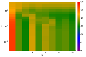
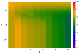
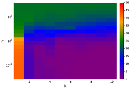
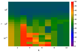
Suppose that we wish to recover a sparse regressor in the synthetic setting described in our numerical experiments, where the ground truth is $k_{\text{true}}=5$-sparse, with autocorrelation $\rho=0.3$ and signal-to-noise ration $\nu=1$ (these parameters are formally defined in Section 5.1.1), and we have a test set of $n_{\text{test}}=10,000$ observations drawn from the same underlying stochastic process to measure test-set performance. In accordance with the standard LOOCV paradigm, we evaluate the LOOCV error for each $k$ and each $\gamma$ log-uniformly distributed on $[10^{-3},10^{3}]$, using the Generalized Benders Decomposition scheme developed by Bertsimas and Van Parys (2020) to solve each MIO to optimality, and selecting the hyperparameter combination with the lowest LOOCV error.

Figure 1 depicts each hyperparameter combination’s leave-one-out (left) and test (right) error, in an overdetermined setting where $n=50,p=10$ (top) and an underdetermined setting where $n=10,p=50$ (bottom). In the overdetermined setting, the LOOCV paradigm performs well: a model trained by minimizing LOOCV attains a test error within $0.6\%$ of the (unknowable) test minimum. However, in the underdetermined setting, LOOCV performs poorly: a model trained by minimizing the LOOCV error attains a test error $19.6\%$ larger than the test set minimum, and seven orders of magnitude larger than its LOOCV estimator. This occurs because the LOOCV estimator is a noisy and high-variance estimator, particularly in underdetermined settings (c.f. Hastie et al. 2009, Chap 7.10). Therefore, its minimum disappoints significantly on a test set.

Figure 1: Leave-one-out (left) and test (right) error for varying $k$ and $\gamma$, for an overdetermined setting (top, $n=50,p=10$) and an underdetermined setting (bottom, $n=10,p=50$). In the overdetermined setting, the leave-one-out error is a good estimate of the test error for most values of parameters $(\gamma,k)$. In contrast, in the underdetermined setting, the leave-one-out is a poor approximation of the test error, and estimators that minimize the leave-one-out error ($\gamma\to 0$, $k=10$) significantly disappoint out-of-sample.

1.2 Literature Review

Our work falls at the intersection of four areas of the optimization and machine learning literature typically considered in isolation. First, hyperparameter selection techniques for optimizing the performance of a machine learning model by selecting hyperparameters that perform well on a validation set. Second, bilevel approaches that reformulate and solve hyperparameter selection problems as bilevel problems. Third, distributionally robust optimization approaches that guard against out-of-sample disappointment when making decisions in settings with limited data. Finally, perspective reformulation techniques for mixed-integer problems with logical constraints. To put our contributions into context, we now review all four areas of the literature.

Hyperparameter Selection Techniques for Machine Learning Problems:

A wide variety of hyperparameter selection techniques have been proposed for machine learning problems such as sparse regression, which follow the same meta-approach: given a set of hyperparameters $\mathcal{L}:=\{(\gamma,k)\}$, we select a combination $(\gamma^{\star},k^{\star})$ which approximately minimize a validation metric $h(\gamma,k)$. Perhaps the most popular approach within this paradigm is grid search (Larochelle et al. 2007), wherein we let $\mathcal{L}:=\{\gamma_{1},\gamma_{2},\ldots,\gamma_{L}\}\times\{k_{1},\ldots,k_{L}\}$ and minimize a validation metric by evaluating it for each $(\gamma,k)\in\mathcal{L}$ separately. Unfortunately, this involves solving a number of training problems exponential in the number of hyperparameters to obtain a solution, i.e., suffers from a curse of dimensionality.

Originally proposed to break this curse of dimensionality, random search (c.f. Bergstra and Bengio 2012) has since emerged as a viable competitor to grid search. In random search, we let $\mathcal{L}$ be a random sample from a space of valid hyperparameters, e.g., a uniform distribution over $[10^{-3},10^{3}]\times[p]$ for sparse regression. Remarkably, in settings with many hyperparameters, random search usually outperforms grid search for a given budget on the number of training problems that can be solved, because validation functions often have a lower effective dimension than the number of hyperparameters present in the model (Bergstra and Bengio 2012). However, grid search remains competitive for problems with a small number of hyperparameters, such as sparse regression.

We point out that current approaches for hyperparameter selection are akin to existing methods for multi-objective mixed-integer optimization. While there has been recent progress in improving multi-objective algorithms for mixed-integer linear programs (Lokman and Köksalan 2013, Stidsen et al. 2014), a direct application of these methods might be unnecessarily expensive. Indeed, these approaches seek to compute the complete efficient frontier (Boland et al. 2015a, b) (i.e., solve problems for all possible values of the regularization parameter), whereas we are interested in only the combination of parameters that optimize a well-defined metric (e.g., LOOCV). As we show in this work, the leave-one-out information can be exploited to speed up the algorithms substantially.

Bilevel Optimization for Hyperparameter Selection:

In a complementary direction, several authors have proposed selecting hyperparameters via bilevel optimization (see Beck and Schmidt 2021, for a general theory), since Bennett et al. (2006) recognized that cross-validation is a special case of bilevel optimization. Therefore, we can minimize the LOOCV error in sparse regression by invoking bilevel techniques. Unfortunately, this approach seems intractable in both theory and practice (Ben-Ayed and Blair 1990, Hansen et al. 1992). Indeed, standard bilevel approaches such as dualizing the lower-level problem give rise to non-convex quadratically constrained integer problems which, in preliminary experiments, we could not solve to optimality with even ten features.

Although slow in its original implementations, several authors have proposed making hyperparameter optimization more tractable by combining bilevel optimization with tractable modeling paradigms to obtain locally optimal sets of hyperparameters. Among others, Sinha et al. (2020) recommends taking a gradient-based approximation of the lower-level problem and thereby reducing the bilevel problem to a single-level problem, Okuno et al. (2021) advocates selecting hyperparameters by solving the KKT conditions of a bilevel problem, and Ye et al. (2022) proposes solving bilevel hyperparameter problems via difference-of-convex methods to obtain a stationary point.

Specializing our review to regression, two recent works aim to optimize the performance of regression models on a validation metric. First, Takano and Miyashiro (2020) proposes optimizing the $k$-fold validation loss, assuming all folds share the same support. Unfortunately, although their assumption improves their method’s tractability, it may lead to subpar statistical performance. Second, Stephenson et al. (2021) proposes minimizing the leave-one-out error in ridge regression problems (without sparsity constraints) and demonstrates that the upper-level objective is often quasi-convex in $\gamma$, which implies first-order methods can often optimize the leave-one-out error. Unfortunately, as we observed in our motivating example and will observe in our numerical results, this result does not appear to hold under a sparsity constraint. Indeed, datasets with one locally optimal $\gamma$ can have many locally optimal $(\gamma,k)$.

Mitigating Out-Of-Sample Disappointment:

The overarching goal of data-driven decision-making procedures, such as sparse regression, is to use historical data to design models that perform well on unseen data drawn from the same underlying stochastic process (King and Wets 1991). Indeed, the original justification for selecting hyperparameters by minimizing a validation metric was that validation metrics are conceptually simple and provide more accurate estimates of out-of-sample performance than the training error (Stone 1974). We now review the literature on cross-validation and related concepts in the context of mitigating out-of-sample disappointment.

From a statistical learning perspective, there is significant literature on quantifying the out-of-sample performance of models with respect to their training and validation error, originating with the seminal works by Vapnik (1999) on VC-dimension and Bousquet and Elisseeff (2002) on algorithmic stability theory. As noted, for instance, by Ban and Rudin (2019), algorithm stability bounds are generally preferable because they are a posteriori bounds with tight constants that depend on only the problem data, while VC-dimension bounds are a priori bounds that depend on computationally intractable constants like Rademacher averages. Irrespective, the conclusion from both streams of work is that simpler and more stable models tend to disappoint less out-of-sample.

More recently, the statistical learning theory literature has been connected to the distributionally robust optimization literature by Ban and Rudin (2019), Gupta and Rusmevichientong (2021) among others. Ban and Rudin (2019) propose solving newsvendor problems by designing decision rules that map features to an order quantity and obtain finite-sample guarantees on the out-of-sample cost of newsvendor policies in terms of the in-sample cost. Even closer to our work, Gupta and Rusmevichientong (2021) proposes correcting solutions to high-dimensional problems by invoking Stein’s lemma to obtain a Stein’s Unbiased Risk Estimator (SURE) approximation of the out-of-sample disappointment and demonstrates that minimizing their bias-corrected training objective generates models that outperform sample-average approximation models out-of-sample.

Perspective Reformulation Techniques:

Many works in the mixed-integer literature have proposed obtaining tight convex relaxations of logically constrained problems by leveraging the fact that the convex closure of a separable convex function under logical constraints can be defined in terms of the convex function’s perspective function. This perspective reformulation technique was originally proposed by Frangioni and Gentile (2006) (see also Aktürk et al. (2009) and Günlük and Linderoth (2010)), building upon insights generated by Ceria and Soares (1999), and is one of the most popular modeling techniques in the mixed-integer nonlinear optimization literature.

More recently, the perspective reformulation technique has culminated in a line of work that, broadly speaking, involves taking the convex hull of certain substructures that appear in mixed-integer problems, such as sparse regression, and designing compact formulations where these convex hulls appear naturally after taking a Boolean relaxation. For instance, Han et al. (2020) derive the convex hulls of bivariate functions under logical constraints, and leverage these convex hulls to design mixed-integer semidefinite formulations with very tight Boolean relaxations. For brevity, we refer to Atamtürk and Gómez (2019, 2020), Bertsimas et al. (2021) for detailed reviews of perspective and related convex relaxations, and their application to sparse regression.

1.3 Structure

The rest of the paper is laid out as follows:

• In Section 2, we specialize a probabilistic generalization bound on the test set error of a machine learning model in terms of its leave-one-out error and its stability to sparse regression. We also propose minimizing this generalization bound, rather than the leave-one-out error itself, to mitigate out-of-sample disappointment.

• In Section 3, we observe that the generalization bound is potentially expensive to evaluate, because computing it involves solving up to $n+1$ MIOs, and accordingly develop tractable lower and upper bounds on the generalization error that can be computed without solving any MIOs.

• In Section 4, we propose an efficient coordinate descent scheme for identifying locally optimal hyperparameters with respect to the generalization error. Specifically, in Section 4.1, we develop an efficient scheme for minimizing the confidence-adjusted leave-one-out error with respect to $k$, and in Section 4.2, we propose a scheme for optimizing with respect to $\gamma$.

• In Section 5, we benchmark our proposed approaches numerically on both synthetic and real datasets. On synthetic datasets, we find that confidence adjustment significantly improves the accuracy of our regressors with respect to identifying the ground truth. Across a suite of $13$ real datasets, we find that our confidence-adjusted cross-validation procedure improves the relative out-of-sample performance of our regressors by $4\%$, on average. Moreover, the proposed approach leads to 50-80% improvements over standard grid search techniques without sacrificing solution quality.

Notation

We let non-boldface characters such as $b$ denote scalars, lowercase bold-faced characters such as $\bm{x}$ denote vectors, uppercase bold-faced characters such as $\bm{A}$ denote matrices, and calligraphic uppercase characters such as $\mathcal{Z}$ denote sets. We let $[n]$ denote the running set of indices $\{1,\dots,n\}$, and $\|\bm{x}\|_{0}:=|\{j:x_{j}\neq 0\}|$ denote the $\ell_{0}$ pseudo-norm, i.e., the number of non-zero entries in $\bm{x}$. Finally, we let $\bm{e}$ denote the vector of ones, and $\bm{0}$ denote the vector of all zeros.

We also invoke matrix operators. We let $\langle\cdot,\cdot\rangle$ denote the Frobenius inner product between two matrices of the same dimension, and $\bm{X}^{\dagger}$ denote the Moore-Penrose pseudoinverse of a matrix $\bm{X}$. If $\bm{x}\neq\bm{0}$ is a vector, then $\bm{x}^{\dagger}=\frac{\bm{x}^{\top}}{\bm{x}^{\top}\bm{x}}$; see Horn and Johnson (1985) for an overview of matrix operators.

Finally, we repeatedly use notation commonplace in the supervised learning literature. We consider a setting where we observe covariates $\bm{X}:=(\bm{x}_{1},\ldots,\bm{x}_{n})\in\mathbb{R}^{n\times p}$ and response data $\bm{y}:=(y_{1},\ldots y_{n})\in\mathbb{R}^{n}$. We say that $(\bm{X},\bm{y})$ is a training set, and let $\bm{\beta}$ denote a regressor fitted on this training set. In leave-one-out cross-validation, we are also interested in the behavior of $\bm{\beta}$ after we leave out one data point from the training set. We let $(\bm{X}^{(i)},\bm{y}^{(i)})$ denote the training set with the $i$th data point left out, and denote by $\bm{\beta}^{(i)}$ the regressor obtained after leaving out the $i$th point.

2 Generalization Bounds on the Test-Set Error

In this section, we formulate the problem of minimizing the leave-one-out cross-validation error for sparse regression in Section 2.1. Further, we improve the formulation in Section 2.2 by recalling a useful generalization bound on the test set error in terms of the model’s stability, due to Bousquet and Elisseeff (2002), and proposing to minimize this bound, rather than the LOOCV error itself.

2.1 Preliminaries

Consider the leave-one-out cross-validation (LOOCV) error (c.f. Stone 1974, Allen 1974) for sparse ridge regression, as defined by the following function:

$$h(\gamma,k)=\frac{1}{n}\sum_{i=1}^{n}\left(y_{i}-\bm{x_{i}}^{\top}\bm{\beta}^{(i)}(\gamma,k)\right)^{2}\ \text{s.t.}\ \bm{\beta}^{(i)}(\gamma,k)\in\argmin_{\bm{\beta}\in\mathbb{R}^{p}:\ \|\bm{\beta}\|_{0}\leq k}\ \frac{\gamma}{2}\|\bm{\beta}\|_{2}^{2}+\|\bm{X}^{(i)}\bm{\beta}-\bm{y}^{(i)}\|_{2}^{2}\ \forall i\in[n],$$

where we take each $\bm{\beta}^{(i)}$ to be the unique minimizer of the $i$th fold training problem for convenience.

$$\text{Moreover, given $i\in[n]$, we let}\quad h_{i}(\gamma,k):=\left(y_{i}-\bm{x_{i}}^{\top}\bm{\beta}^{(i)}(\gamma,k)\right)^{2}$$ (3)

denote the $i$th partial leave-one-out error, with $1/n\sum_{i=1}^{n}h_{i}(\gamma,k)=h(\gamma,k)$.

The LOOCV error is a widely-used estimator of the test error, because it is an approximately unbiased estimator for a fixed hyperparameter combination (c.f. Hastie et al. 2009, Chap 7.10). Unfortunately, as mentioned in Section 1, it suffers from two major drawbacks. First, the optimized LOOCV error may be an overly optimistic estimator of the test error, particularly if $n<p$, and thus estimators obtained by selecting $(\gamma,k)\in\argmin h(\gamma,k)$ may lead to significant out-of-sample disappointment. Second, for a fixed $\bar{\gamma}$, computing $h(\bar{\gamma},k)=1/n\sum_{i=1}^{n}h_{i}(\bar{\gamma},k)$ requires solving $n$ MIOs with $p$ decision variables to optimality; thus, optimizing $\min_{k\in[p]}h(\bar{\gamma},k)$ using grid search requires solving $np$ MIOs to optimality, which is often prohibitively expensive. Accordingly, we now quantify the extent to which it may disappoint out-of-sample as a function of the LOOCV error and a model’s stability, with a view to improve its test-set performance.

2.2 Hypothesis Stability Generalization Bounds

Let $\mathcal{S}$ denote a random draw over the test set, $\mathcal{T}$ denote a training set of size $n$, and $\bm{\beta}^{\star}$ be a regressor trained over the entire training set with a fixed but arbitrary set of hyperparameters $(k,\gamma)$. Then, according to Bousquet and Elisseeff (2002, Theorem 11), under appropriate assumptions, Chebyshev’s inequality implies the following confidence bound holds with probability at least $1-\delta$:

$$\frac{1}{|\mathcal{S}|}\sum_{i\in\mathcal{S}}(y_{i}-\bm{x}_{i}^{\top}\bm{\beta}^{\star})^{2}\leq\frac{1}{n}\sum_{i\in\mathcal{T}}h_{i}(\gamma,k)+\sqrt{\frac{M^{2}+6Mn\mu_{h}}{2n\delta}},$$ (4)

where $M$ is an upper bound on the loss function $\ell(\bm{x}_{i}^{\top}\bm{\beta}^{\star},y_{i})=(y_{i}-\bm{x}_{i}^{\top}\bm{\beta}^{\star})^{2}$ for any $i$—which we approximate via $\max_{i\in\mathcal{T}}y_{i}^{2}$—and $\mu_{h}$ is the hypothesis stability of our sparse learning algorithm (Bousquet and Elisseeff 2002, Definition 3), which we approximate via:

$$\mu_{h}:=\max_{i\in[n]}\frac{1}{n}\sum_{j=1}^{n}\left|(y_{j}-\bm{x_{j}^{\top}\bm{\beta}^{\star}})^{2}-(y_{j}-\bm{x_{j}^{\top}\beta}^{(i)})^{2}\right|,$$ (5)

i.e., the worst-case average absolute change in the learning loss after leaving out the $i$th data point.

Therefore, to account for out-of-sample disappointment when cross-validating sparse regression models, we propose selecting hyperparameters by solving the following optimization problem:

$$(\gamma,k)\in\argmin_{\gamma\in\mathbb{R}_{+},k\in[p]}g(\gamma,k).\quad\text{Where}\quad g(\gamma,k):=\frac{1}{n}\sum_{i\in\mathcal{T}}h_{i}(\gamma,k)+\sqrt{\frac{M^{2}+6Mn\mu_{h}(\gamma,k)}{2n\delta}}$$ (6)

denotes the confidence-adjusted cross-validation error for a user-specified confidence level $\delta>0$. Accordingly, from a multi-objective optimization perspective, our approach is equivalent to selecting a hyperparameter combination $(\gamma,k)$ on the Pareto frontier of hyperparameters with the smallest hypothesis stability score and the least LOOCV error, using the confidence level $\delta$ to obtain a scalarization weight (see also Ehrgott 2005, for a general theory of multi-objective optimization).

If $\delta\rightarrow\infty$ or $n\to\infty$, then $g(\gamma,k)=h(\gamma,k)$ is simply the leave-one-out error, while as $\delta\rightarrow 0$ we select the most stable regressor in the sense of Bousquet and Elisseeff (2002), rather than the regressor that minimizes the LOOCV error. The former case arises naturally in overdetermined settings if we fix $\delta$ and let $n\rightarrow\infty$, because sparse linear regression models become more stable as $n$ increases (see, e.g., Bertsimas and Van Parys 2020, Gamarnik and Zadik 2022). On the other hand, the latter case is not well studied in the sparse regression literature, but has essentially been explored in the portfolio optimization literature (c.f. DeMiguel and Nogales 2009), where it has been found to be effective in settings with high ambiguity.

We conclude this section by noting that one could alternatively minimize a bound that concentrates exponentially via McDiarmind’s inequality (Bousquet and Elisseeff 2002, Theorem 12). Unfortunately, this exponential bound includes a constant term related to the uniform stability (Bousquet and Elisseeff 2002, Definition 6) of our regressors which, in preliminary numerical experiments, we found was often so large that it made the exponential bound vacuous.

3 Convex Relaxations of Leave-one-out and Its Confidence-Adjusted Variants

In the previous section, we proposed selecting $k,\gamma$ by minimizing the leave-one-out cross-validation error $g$, as defined in Problem (6). From an optimization perspective, this proposal might appear to be numerically challenging to implement, because evaluating $g$ requires solving $n$ MIOs. Inspired by this challenge, in this section, we develop tractable upper and lower approximations of $g$ which can be evaluated at a given $(\gamma,k)$ without solving any MIOs. The core workhorse of our approach is a method for constructing bounds $\underline{\xi},\overline{\xi}$ such that $\underline{\xi}\leq\bm{x^{\top}\beta}^{(i)}\leq\overline{\xi}$, which we propose in Section 3.1 and extend straightforwardly to bound the $k$-fold spread. We then leverage this insight to bound

$$h_{i}=(y_{i}-\bm{x_{i}^{\top}}\bm{\beta}^{(i)})^{2},$$ (7)

and $$\upsilon_{i,j}=(y_{j}-\bm{x_{j}^{\top}}\bm{\beta}^{(i)})^{2}$$ (8)

in Sections 3.2 and 3.3 respectively, which allows us to bound $g$ from above and below without solving MIOs, and leads to the coordinate descent approach we develop in Section 4.

3.1 Bounding Prediction Spread

Given any $0<2\epsilon<\gamma$, Problem (1) admits the conic quadratic relaxation:

$$\zeta_{\text{persp}}=\min_{\bm{\beta}\in\mathbb{R}^{p},\bm{z}\in[0,1]^{p}}\quad\|\bm{y}-\bm{X}\bm{\beta}\|_{2}^{2}+\epsilon\|\bm{\beta}\|_{2}^{2}+\frac{\gamma-2\epsilon}{2}\sum_{i=1}^{p}\frac{\beta_{i}^{2}}{z_{i}}\quad\text{s.t.}\quad \sum_{i=1}^{p}z_{i}\leq k,$$ (9)

which is also known as the perspective relaxation (c.f. Günlük and Linderoth 2010). Observe that if integrality constraints $\bm{z}\in\{0,1\}^{p}$ are added to (9), then the resulting mixed-integer optimization problem (MIO) is a reformulation of (1), where the logical constraints $z_{i}=0$ if $\beta_{i}=0\ \forall i\in[p]$ are implicitly imposed via the domain of the perspective function $\beta_{i}^{2}/z_{i}$. Moreover, if $\epsilon\to 0$, the optimal objective $\zeta_{\text{persp}}$ of (9) often provides tight lower bounds on the objective value of (1) (Bertsimas and Van Parys 2020), and the optimal solution $\bm{\beta}_{\text{persp}}^{*}$ is a good estimator in its own right. As we establish in our main theoretical result, the perspective relaxation can also be used to obtain accurate approximations and lower/upper bounds of the stability terms $\upsilon_{i,j}(\gamma,k)$ defined in (8).

Theorem 3.1

Given any vector $\bm{x}\in\mathbb{R}^{p}$, any $0<2\epsilon<\gamma$ and any bound

$$\bar{u}\geq\min_{\bm{\beta}\in\mathbb{R}^{p}}\;\|\bm{X}\bm{\beta}-\bm{y}\|_{2}^{2}+\frac{\gamma}{2}\|\bm{\beta}\|_{2}^{2}\text{ s.t. }\;\|\bm{\beta}\|_{0}\leq k,$$ (10)

the inequalities

$$\bm{x^{\top}\beta}_{persp}^{*}-\sqrt{\left(\bar{u}-\zeta_{\text{persp}}\right)\bm{x^{\top}}\left(\bm{X^{\top}X}+\epsilon\mathbb{I}\right)^{-1}\bm{x}}\leq\bm{x}^{\top}\bm{\beta}_{MIO}^{*}\leq\bm{x^{\top}\beta}_{persp}^{*}+\sqrt{\left(\bar{u}-\zeta_{\text{persp}}\right)\bm{x^{\top}}\left(\bm{X^{\top}X}+\epsilon\mathbb{I}\right)^{-1}\bm{x}}$$

hold, where $\bm{\beta}_{MIO}^{*}$ is an optimal solution of (10) and $\bm{\beta}_{persp}^{*}$ is optimal to (9).

Proof 3.2

Outline of the proof of Theorem 3.1 We now describe the main idea of the proof and defer the details to Appendix 7.1. Consider the non-convex problem

$$u=\min_{\bm{\beta}\in\mathbb{R}^{p}} \|\bm{X}\bm{\beta}-\bm{y}\|_{2}^{2}+\frac{\gamma}{2}\|\bm{\beta}\|_{2}^{2}\ \text{s.t.}\ \|\bm{\beta}\|_{0}\leq k$$ (11)

and, given any $0<2\epsilon<\gamma$ and $\bm{x}\in\mathbb{R}^{p}\setminus\{\bm{0}\}$, consider the following perspective reformulation parametrized by $\xi\in\mathbb{R}$

$$\phi(\xi)=\min_{\bm{\beta}\in\mathbb{R}^{p},\bm{z}\in[0,1]^{p}}\; \|\bm{X}\bm{\beta}-\bm{y}\|_{2}^{2}+\epsilon\|\bm{\beta}\|_{2}^{2}+\frac{\gamma-2\epsilon}{2}\sum_{j=1}^{p}\frac{\beta_{j}^{2}}{z_{j}}\ \text{s.t.}\ \sum_{j=1}^{p}z_{j}\leq k,\ \bm{x^{\top}\beta}=\xi.$$

Then, given any upper bound $\bar{u}\geq u$ and lower bound $\underline{\phi}(\xi)\leq\phi(\xi)$, if $\underline{\phi}(\xi)>\bar{u}$ we know that setting $\bm{x^{\top}\beta}=\xi$ is not possible in any optimal solution of (11), and we say that value $\xi$ is not admissible. We then use duality to construct an interval $[\underline{\xi},\bar{\xi}]$ outside which all values are not admissible.

Extension to Bounding the $k$-fold Spread:

In this paper, our main goal is optimizing the confidence-adjusted leave-one-out error. However, bounding the spread of the $k$-fold cross-validation error may be of independent interest. One could achieve this by bounding the spread of each data point left out separately, but this is potentially suboptimal, because it does not account for the fact that the solutions to the MIO and the perspective relaxation should be equal for each datapoint. Therefore, we now obtain a tighter bound on the $k$-fold cross-validation spread, using a similar proof technique as in the proof of Theorem 3.1:

Theorem 3.3

Given any matrix $\bm{W}\in\mathbb{R}^{p\times q}$, where $q\geq 1$, any $0<2\epsilon<\gamma$ and any bound

$$\bar{u}\geq\min_{\bm{\beta}\in\mathbb{R}^{p}}\;\|\bm{X}\bm{\beta}-\bm{y}\|_{2}^{2}+\frac{\gamma}{2}\|\bm{\beta}\|_{2}^{2}\text{ s.t. }\;\|\bm{\beta}\|_{0}\leq k,$$

the inequality

$$(\beta^{\star}_{\text{persp}}-\bm{W}^{\dagger}\bm{W}\bm{\beta}^{\star}_{\text{MIO}})^{\top}\left(\bm{X}^{\top}\bm{X}+\varepsilon\mathbb{I}\right)(\beta^{\star}_{\text{persp}}-\bm{W}^{\dagger}\bm{W}\bm{\beta}^{\star}_{\text{MIO}})\leq(\bar{u}-\zeta_{\text{persp}}).$$ (12)

holds, where $\bm{\beta}_{MIO}^{*}$ is an optimal solution of (10), $\bm{\beta}_{persp}^{*}$ is optimal to (9), and $\bm{W}^{\dagger}$ denotes the Moore-Penrose pseudoinverse of $\bm{W}$.

Proof 3.4

Proof of Theorem 3.3 We now sketch the proof outline and defer the details to Appendix 8.

The overall proof follows similarly to the proof of Theorem 3.1: we construct a perspective relaxation $\phi(\bm{\xi})$ parameterized by $\bm{\xi}$ in which we impose a constraint $\bm{\xi}=\bm{W\beta}$, and use this relaxation to construct an ellipsoid outside which all values of $\bm{\xi}$ are not admissible.

Before we stated Theorem 3.3, we claimed that it gives a potentially tighter bound on the $k$-fold spread than by bounding the spread of each data point left out separately. We now justify this claim: by the Generalized Schur complement lemma (see, e.g., Boyd et al. 1994), our bound on the $k$-fold spread is equivalent to requiring that

$$(\bar{u}-\zeta_{\text{persp}})\left(\bm{X}^{\top}\bm{X}+\varepsilon\mathbb{I}\right)^{-1}\succeq(\beta^{\star}_{\text{persp}}-\bm{W}^{\dagger}\bm{W}\bm{\beta}^{\star}_{\text{MIO}})(\beta^{\star}_{\text{persp}}-\bm{W}^{\dagger}\bm{W}\bm{\beta}^{\star}_{\text{MIO}})^{\top}.$$

Left/ right multiplying this expression by $\bm{W}/\bm{W}^{\top}$ and taking the trace of both sides of the above expression then gives the following (weaker) condition

$$(\bar{u}-\zeta_{\text{persp}})\left\langle\bm{W}\bm{W}^{\top},\left(\bm{X}^{\top}\bm{X}+\varepsilon\mathbb{I}\right)^{-1}\right\rangle\geq\|\bm{W}\beta^{\star}_{\text{persp}}-\bm{W}\bm{\beta}^{\star}_{\text{MIO}}\|_{2}^{2}$$

which is equivalent to applying our leave-one-out bound to each column left out in a $k$-fold split separately. Indeed, if $\bm{W}=\bm{x}^{\top}$, this weaker bound reduces to our leave-one-out bound.

Applicability of Leave-one-out Bound:

We conclude this section with two remarks.

Remark 3.5 (Choice of parameter $\epsilon$)

The role of the parameter $\epsilon$ is to ensure that $\bm{x}$ is in the range of the matrix $\bm{X^{\top}X}+\epsilon\mathbb{I}$. If the matrix $\bm{x}$ is already in the range of $\bm{X}$, as occurs, for instance, after solving a convex relaxation of the training problem without any observations omitted, then one should set $\epsilon=0$ and replace the inverse in Theorem 3.1’s bound with a pseudoinverse, as lower values of $\epsilon$ result in stronger perspective relaxations. However, this is not possible in general; for instance, $\bm{x}_{i}$ need not be in the range of $\bm{X}^{(i)}$ in highly underdetermined settings.

Remark 3.6 (Intuition)

Theorem 3.1 states that $\bm{x}^{\top}\bm{\beta}_{MIO}^{*}\approx\bm{x^{\top}\beta}_{persp}^{*}$, where the approximation error is determined by two components. The quantity $\sqrt{\bar{u}-\zeta_{\text{persp}}}$ is related to the strength of the perspective relaxation, with a stronger relaxation resulting in a better approximation. The quantity $\sqrt{\bm{x^{\top}}\left(\bm{X^{\top}X}+\epsilon\mathbb{I}\right)^{-1}\bm{x}}$ is related to the likelihood that $\bm{x}$ is generated from the same distribution as the rows of $\bm{X}$, with larger likelihoods resulting in better approximations. Indeed, if $n>p$, each column of $\bm{X}$ has $0$ mean but has not been standardized, and each row of $\bm{X}$ is generated iid from a multivariate Gaussian distribution, then $\frac{n(n-1)}{n+1}\bm{x^{\top}}\left(\bm{X^{\top}X}\right)^{-1}\bm{x}\sim T^{2}(p,n-1)$ is Hotelling’s two-sample T-square test statistic (Hotelling 1931), used to test whether $\bm{x}$ is generated from the same Gaussian distribution. Note that if $\bm{x}$ is drawn from the same distribution as the rows of $\bm{X}$ (as may be the case in leave-one-out cross-validation), then $\mathbb{E}\left[\bm{x^{\top}}\left(\bm{X^{\top}X}\right)^{-1}\bm{x}\right]=\frac{p(n+1)}{n(n-p-2)}$.

In the rest of this section, we discuss how to leverage Theorem 3.1 to approximate and bound the confidence-adjusted LOOCV error $g$ without incurring the cost of solving $n$ MIOs. We treat the LOOCV error and the hypothesis stability terms in $g$ separately, as it is straightforward to bound $g$ given bounds on both these terms. We also propose some refinements to Theorem 3.1, which sometimes allow us to obtain tighter bounds.

3.2 Approximating The Leave-One-Out Error

Applying Theorem 3.1 to the problem

$$\bar{u}^{(i)}\geq\min_{\bm{\beta}\in\mathbb{R}^{p}}\;\|\bm{X}^{(i)}\bm{\beta}-\bm{y}^{(i)}\|_{2}^{2}+\frac{\gamma}{2}\|\bm{\beta}\|_{2}^{2}\text{ s.t. }\;\|\bm{\beta}\|_{0}\leq k,$$

where $\bm{X}^{(i)}$ and $\bm{y}^{(i)}$ are the model matrix and response vector after leaving out the $i$th datapoint, and $\bm{x_{i}}$ denotes the omitted column of $\bm{X}$, we have the bounds

$$\underline{\xi}:=\bm{x_{i}^{\top}}\bm{\beta}_{persp}^{*}-\sqrt{\bm{x_{i}^{\top}}\left(\bm{X}^{(i)^{\top}}\bm{X}^{(i)}+\epsilon\mathbb{I}\right)^{-1}\bm{x_{i}}\left(\bar{u}^{(i)}-\zeta^{i}\right)},$$

$$\bar{\xi}:=\bm{x_{i}^{\top}}\bm{\beta}_{persp}^{*}+\sqrt{\bm{x_{i}^{\top}}\left(\bm{X}^{(i)^{\top}}\bm{X}^{(i)}+\epsilon\mathbb{I}\right)^{-1}\bm{x_{i}}\left(\bar{u}^{(i)}-\zeta^{i}\right)}$$

where $0<2\epsilon<\gamma$ and $\underline{\xi}\leq\bm{x_{i}^{\top}}\bm{\beta}_{MIO}^{*}\leq\bar{\xi}$. We can use these bounds to bound functions $h_{i}(\gamma,k)$.

Corollary 3.7

We have the following bounds on the $i$th partial LOOCV error:

$$\max\left((y_{i}-\underline{\xi})^{2},(y_{i}-\bar{\xi})^{2}\right)\geq h_{i}(\gamma,k)\geq\begin{cases}(y_{i}-\underline{\xi})^{2}\quad&\text{if}\ y_{i}<\underline{\xi}\\ 0\quad&\text{if}\ y_{i}\in[\underline{\xi},\bar{\xi}],\\ (\bar{\xi}-y_{i})^{2}\quad&\text{if}\ y_{i}>\bar{\xi}.\end{cases}$$ (13)

Remark 3.8 (Relaxation Tightness)

If the perspective relaxation is tight, then $\underline{\xi}=\bar{\xi}=\bm{x_{i}^{\top}}\bm{\beta}_{persp}^{*}$, and Corollary 3.7’s bounds on the leave-one-out error are definitionally tight. Otherwise, as pointed out in Remark 3.6, (13)’s bound quality depends explicitly on the tightness of the perspective relaxation and on how close the features $\bm{x}_{i}$ are to the rest of the data.

We now demonstrate that we can use the same technique to bound the $k$-fold CV error, which may be of independent interest, before returning our attention to LOOCV for the rest of the paper.

Corollary 3.9 (Extension to Bounding the $k$-fold Error)

Let $\bm{X}^{(\mathcal{S})},\bm{y}^{(\mathcal{S})}$ denote the model matrix and response vector after leaving out the data points indexed by the set $\mathcal{S}$, and $\bm{X}^{\mathcal{S}},\bm{y}^{\mathcal{S}}$ denote the omitted features and responses. Further, let

$$\bar{u}^{(\mathcal{S})}\geq\min_{\bm{\beta}\in\mathbb{R}^{p}}\;\|\bm{X}^{(\mathcal{S})}\bm{\beta}-\bm{y}^{(\mathcal{S})}\|_{2}^{2}+\frac{\gamma}{2}\|\bm{\beta}\|_{2}^{2}\text{ s.t. }\;\|\bm{\beta}\|_{0}\leq k,$$

be an upper bound on the relevant training problem, $\zeta^{(\mathcal{S})}$ denote the optimal value of this problem’s perspective relaxation, and $\beta_{\text{persp}}^{(\mathcal{S})\star}$ denote an optimal solution to this perspective relaxation. Then, maximizing/minimizing the following quadratically constrained problem yields valid upper/lower bounds on the partial $k$-fold cross-validation error, $\|\bm{y}^{\mathcal{S}}-\bm{X}^{\mathcal{S}}\bm{\beta}^{(\mathcal{S})}_{\text{MIO}}\|_{2}^{2}$

$$\max_{\bm{\beta}\in\mathbb{R}^{p}}/\min_{\bm{\beta}\in\mathbb{R}^{p}}\quad \|\bm{y}^{\mathcal{S}}-\bm{X}^{\mathcal{S}}\bm{\beta}\|_{2}^{2}$$

s.t. $$(\beta_{\text{persp}}^{(\mathcal{S})\star}-\bm{X}^{\mathcal{S}{\dagger}}\bm{X}^{\mathcal{S}}\bm{\beta})^{\top}\left(\bm{X}^{(\mathcal{S})\top}\bm{X}^{(\mathcal{S})}+\varepsilon\mathbb{I}\right)(\beta_{\text{persp}}^{(\mathcal{S})\star}-\bm{X}^{\mathcal{S}{\dagger}}\bm{X}^{\mathcal{S}}\bm{\beta})\leq(\bar{u}^{(\mathcal{S})}-\zeta_{\text{persp}}^{(\mathcal{S})})$$

Remark 3.10 (Computability of k-fold bounds)

Observe that a lower bound on the $k$-fold error can easily be computed using second-order cone optimization, while an upper bound can be computed by noticing that the above maximization problem is a trust region problem, which can be formulated as a semidefinite problem and solved efficiently (Hazan and Koren 2016). One could further tighten these bounds by imposing a sparsity constraint on $\bm{\beta}$, but this may not be practically tractable.

Implications of Leave-One-Out Bound:

Corollary 3.7 implies that we may obtain a valid upper and lower bound on $h$ at a given hyperparameter combination $\gamma,k$ after solving $n$ perspective relaxations and computing $n$ terms of the form $\sqrt{\bm{x_{i}^{\top}}\left(\bm{X}^{(i)^{\top}}\bm{X}^{(i)}+\epsilon\mathbb{I}\right)^{-1}\bm{x_{i}}}$. Notably, the latter terms do not depend on $\gamma$ and $k$ and thus can be computed a priori before solving (6).

A drawback of Corollary 3.7 is that if $\bm{x_{i}^{\top}}\bm{\beta}_{persp}^{*}\approx y_{i}$, i.e., the prediction of the perspective relaxation (without point $i$) is close to the response associated with point $i$, then Corollary 3.7’s lower bound is $0$. We now propose a different bound on $h_{i}$, which is sometimes effective in this circumstance.

First, let us define the function $f(\gamma,k)$ to be the in-sample training error with parameters $(\gamma,k)$,

$$f(\gamma,k):=1/n\sum_{i=1}^{n}(y_{i}-\bm{x_{i}}^{\top}\bm{\beta}(\gamma,k))^{2}\quad\text{s.t.}\quad\bm{\beta}(\gamma,k)\in\arg\min_{\bm{\beta}\in\mathbb{R}^{p}:\ \|\bm{\beta}\|_{0}\leq k}\ \frac{\gamma}{2}\|\bm{\beta}\|_{2}^{2}+\|\bm{X}\bm{\beta}-\bm{y}\|_{2}^{2},$$

and let $f_{i}(\gamma,k):=\left(y_{i}-\bm{x_{i}}^{\top}\bm{\beta}(\gamma,k)\right)^{2}$ denote the $i$th training error, with $1/n\sum_{i=1}^{n}f_{i}(\gamma,k)=f(\gamma,k)$. Observe that evaluating $h(\gamma,k)$ involves solving $n$ MIOs, while evaluating $f$ requires solving one.

Proposition 3.11

For any $\gamma\geq 0$ and any $k\in[p]$, $f_{i}(\gamma,k)\leq h_{i}(\gamma,k)$. Moreover, $f(\gamma,k)\leq h(\gamma,k)$.

Proof 3.12

Proof of Proposition 3.11 We defer the details to Appendix 8.1.

Corollary 3.13

Given any $\gamma_{1}\leq\gamma_{2}$ and $k_{1}\geq k_{2}$, $f(\gamma_{1},k_{1})\leq f(\gamma_{2},k_{2})$ and thus $f(\gamma_{1},k_{1})\leq h(\gamma_{2},k_{2})$.

Next, we develop a stronger bound on the LOOCV error, by observing that our original proof technique relies on interpreting the optimal solution when training on the entire dataset as a feasible solution when leaving out the $i$th data point, and that this feasible solution can be improved to obtain a tighter lower bound. Therefore, given $\bm{z}\in\{0,1\}^{p}$, let us define the function:

$$f^{(i)}(\bm{z}):=\min_{\bm{\beta}\in\mathbb{R}^{p}}\quad\frac{\gamma}{2}\sum_{i\in[p]}\beta_{i}^{2}+\|\bm{X}^{(i)}\bm{\beta}-\bm{y}^{(i)}\|_{2}^{2}\ \text{s.t.}\ \beta_{i}=0\ \text{if}\ z_{i}=0\ \forall i\in[p],$$

to be the optimal training loss (including regularization) when we leave out the $i$th observation and have the binary support vector $\bm{z}$. Then, fixing $\gamma,k$ and letting $u^{*}$ denote the optimal objective value of (31), i.e., the optimal training loss on the entire dataset (including regularization) and $\bm{\beta}^{(i)}(\bm{z})$ denote an optimal choice of $\bm{\beta}$ for this $\bm{z}$, we have the following result:

Proposition 3.14

For any $k$-sparse binary vector $\bm{z}$, the following inequality holds:

$$u^{*}\leq f^{(i)}(\bm{z})+(y_{i}-\bm{x}_{i}^{\top}\bm{\beta}^{(i)}(\bm{z}))^{2}$$ (14)

Proof 3.15

Proof of Proposition 3.14 The right-hand side of this inequality corresponds to the objective value of a feasible solution to (31), while $\bar{u}$ is the optimal objective value of (31).

Corollary 3.16

Let $\bm{z}$ denote a $k$-sparse binary vector. Then, we have the following bound on the $i$-th partial leave-one-out error:

$$h_{i}(\gamma,k)\geq u^{*}-f^{(i)}(\bm{z}).$$ (15)

Proof 3.17

Proof of Corollary 3.16 The right-hand side of this bound is maximized by setting $\bm{z}$ to be a binary vector which minimizes $f^{(i)}(\bm{z})$, and therefore this bound is valid for any $\bm{z}$.

Remark 3.18 (Bound quality)

Observe that bound (15) is at least as strong as $f_{i}(\gamma,k)$ with $\bm{z}$ encoding an optimal choice of support in (31). Indeed, if $\bm{\beta}^{(i)}(\bm{z})$ solves (31), then both bounds agree and equal $h_{i}(\gamma,k)$ but otherwise (15) is strictly stronger. Moreover, since $f_{i}(\gamma,k)$ is typically nonzero, then the bound (15) is positive as well and can improve upon the lower bound in (13). Finally, it is easy to construct an example where the lower bound in (13) is stronger than (15), thus neither lower bound dominates the other.

Remark 3.19 (Computational efficiency)

Computing lower bound (15) for each $i\in[n]$ requires solving at least one MIO, corresponding to (31), which is a substantial improvement over the $n$ MIOs required to compute $h$ but may still be an expensive computation. However, using any lower bound on $u^{*}$, for example, corresponding to the optimal solution of a perspective relaxation, gives valid lower bounds. Therefore, in practice, we suggest using a heuristic instead to bound $h_{i}$ from below, e.g., rounding a perspective relaxation.

3.3 Approximating the Hypothesis Stability

We now leverage Theorem 3.1 to develop bounds on the hypothesis stability:

$$\mu_{h}:=\max_{i\in[n]}\frac{1}{n}\sum_{j=1}^{n}\left|(y_{j}-{\bm{\beta}^{\star}}^{\top}\bm{x}_{j})^{2}-(y_{j}-\bm{\beta}^{(i)}\bm{x}_{j})^{2}\right|.$$

To develop these bounds, let us denote by $u$ the optimal value of Problem (11), i.e., the optimal value of a sparse regression problem run on the entire dataset, let $\zeta$ denote the optimal value of Problem (11)’s perspective relaxation, i.e.,

$$\zeta=\min_{\bm{\beta}\in\mathbb{R}^{p},\bm{z}\in[0,1]^{p}}\; \|\bm{X}\bm{\beta}-\bm{y}\|_{2}^{2}+\frac{\gamma}{2}\sum_{j=1}^{p}\frac{\beta_{j}^{2}}{z_{j}}\ \text{s.t.}\ \sum_{j=1}^{p}z_{j}\leq k,$$

let $\bm{\beta}_{MIO}$ denote an optimal solution to Problem (11) and $\bm{\beta}_{persp}$ denote an optimal solution to its perspective relaxation. Further, let $u^{(i)},\zeta^{(i)}$, $\bm{\beta}^{(i)}_{MIO}$, $\bm{\beta}^{(i)}_{persp}$ be equivalent objects with the $i$th data point left out of the training problem. Then, we have the following corollary to Theorem 3.1:

Corollary 3.20

Let $0<2\epsilon<\gamma$. Then, we have the following bounds on $\bm{x}_{j}^{\top}\bm{\beta}_{\text{MIO}}$ and $\bm{x}_{j}^{\top}\bm{\beta}_{\text{MIO}}$:

$$|\bm{x}_{j}^{\top}\bm{\beta}_{\text{MIO}}-\bm{x}_{j}^{\top}\bm{\beta}_{persp}|\leq \sqrt{\bm{x}_{j}^{\top}\left(\bm{X}^{\top}\bm{X}+\epsilon\mathbb{I}\right)^{-1}\bm{x}_{j}(u-\zeta)},$$ (16)

$$|\bm{x}_{j}^{\top}\bm{\beta}^{(i)}_{MIO}-\bm{x}_{j}^{\top}\bm{\beta}^{(i)}_{persp}|\leq \sqrt{\bm{x}_{j}^{\top}\left(\bm{X}^{(i)\top}\bm{X}^{(i)}+\epsilon\mathbb{I}\right)^{-1}\bm{x}_{j}(u^{(i)}-\zeta^{(i)})}.$$ (17)

Given these bounds, we can produce lower and upper bounds on the quantities $(y_{j}-{\bm{\beta}^{\star}}^{\top}\bm{x}_{j})^{2}$ and $(y_{j}-\bm{\beta}^{(i)}\bm{x}_{j})^{2}$ in essentially the same manner as Corollary 3.7, say $[l_{j},u_{j}]$ and $[l^{(i)}_{j},u_{j}^{(i)}]$.

From Corollary 3.20, we observe that the hypothesis stability $\mu_{h}$ is very similar for $\bm{\beta}^{\star}_{\text{MIO}}$ and $\bm{\beta}^{\star}_{\text{persp}}$, especially when the perspective relaxation is nearly tight. Moreover, as we will observe empirically in Section 5, the cross-validated regressors $\bm{\beta}^{\star}_{\text{MIO}}$ and $\bm{\beta}^{\star}_{\text{persp}}$ behave extremely similarly whenever $n$ is sufficiently large. Therefore, since solving the perspective relaxation is much cheaper than solving a MIO, we use $\bm{\beta}^{\star}_{\text{persp}}$ in lieu of $\bm{\beta}^{\star}_{\text{MIO}}$ for our experiments involving confidence adjustment. However, we can easily construct a lower bound on $\bm{\beta}^{\star}_{\text{MIO}}$ by solving the following linear optimization problem

$$\mu_{h}\geq\min_{\bm{x}\in\mathbb{R}^{n},\bm{Y}\in\mathbb{R}^{n\times n}}\max_{i\in[n]}\frac{1}{n}\sum_{j\in[n]}|x_{i}-Y_{i,j}|\ \text{s.t.}\ \bm{l}\leq\bm{x}\leq\bm{u},Y_{i,j}\in[l_{j}^{(i)},u_{j}^{(i)}]\ \forall i,j\in[n].$$

Moreover, we can construct an upper bound in much the same way after replacing the outer minimization operator with a maximization operator, by solving the following MIO

$$\mu_{h}\leq\max_{\bm{x}\in\mathbb{R}^{n},\bm{z}\in\{0,1\}^{n\times n},\bm{\theta},\bm{Y}\in\mathbb{R}^{n\times n}}\max_{i\in[n]}\quad \frac{1}{n}\sum_{j\in[n]}\theta_{i,j}$$

s.t. $$\theta_{i,j}\geq|x_{i}-Y_{i,j}|,\quad\forall i,j\in[n]$$

$$\theta_{i,j}\leq x_{i}-Y_{i,j}+M(1-z_{i,j}),\theta_{i,j}\leq-x_{i}+Y_{i,j}+Mz_{i,j}$$

$$\bm{l}\leq\bm{x}\leq\bm{u},Y_{i,j}\in[l_{j}^{(i)},u_{j}^{(i)}]\ \forall i,j\in[n],$$

or its Boolean relaxation. Finally, we remark that in some circumstances, we may be willing to evaluate $\bm{\beta}_{MIO}$ exactly, which involves solving one MIO, but not $\bm{\beta}^{(i)}_{MIO}$, which involves solving $n$ MIOs. In this situation, we bound $\mu_{h}$ almost identically, except the bounds on $x_{i}$, which in spirit models $(y_{i}-\bm{x}_{i}^{\top}\bm{\beta}_{MIO})^{2}$, are now tight, and we bound $\mu_{h}$ from above by setting $Y_{i,j}=u_{j}^{(i)}$ if $|u_{j}^{(i)}-x_{i}|\geq|l_{j}^{(i)}-x_{i}|$ and $l_{j}^{(i)}$ otherwise, rather than solving a MIO.

4 Optimizing the Cross-Validation Loss: A Coordinate Descent Approach

In this section, we present an efficient coordinate descent scheme that identifies (approximately) locally optimal hyperparameters $(\gamma,k)$ with respect to the confidence-adjusted LOOCV metric:

$$g(\gamma,k):=\frac{1}{n}\sum_{i=1}^{n}h_{i}(\gamma,k)+\sqrt{\frac{M^{2}+6Mn\mu_{h}(\gamma,k)}{2n\delta}},\\$$ (18)

by iteratively minimizing $k$ and $\gamma$. In the tradition of classical coordinate descent schemes, with initialization $k_{0},\gamma_{0}$, we propose repeatedly solving the following two optimization problems:

$$k_{t}\in\arg\min_{k\in[p]}\quad g(\gamma_{t},k),$$ (19)

$$\gamma_{t+1}\in\arg\min_{\gamma>0}\quad g(\gamma,k_{t}),$$ (20)

until we either detect a cycle or converge to a locally optimal solution. To develop this scheme, in Section 4.1 we propose an efficient technique for solving Problem (18), and in Section 4.2 we propose an efficient technique for (approximately) solving Problem (19). Accordingly, our scheme could also be used to identify an optimal choice of $\gamma$ if $k$ is already known, e.g., in a context where regulatory constraints specify the number of features that may be included in a model.

Our overall approach is motivated by two key observations. First, we design a method that obtains local, rather than global, minima, because $g$ is a highly non-convex function and even evaluating $g$ requires solving $n$ MIOs, which suggests that global minima of $g$ may not be attainable in a practical amount of time at scale. Second, we use coordinate descent to seek local minima because if either $k$ or $\gamma$ is fixed, it is possible to efficiently optimize the remaining hyperparameter with respect to $g$ by leveraging the convex relaxations developed in the previous section.

We remark that in a subset of our numerical experiments, we require that the optimal values of $\gamma$ and $k$ should be contained within the intervals $[\gamma_{\min},\gamma_{\max}]$ and $[k_{\min},k_{\max}]$. For instance, we require that $k_{\max}$ is such that $k_{\max}\log k_{\max}\leq n$ in our experiments in Section 5.5, because Gamarnik and Zadik (2022, Theorem 2.5) demonstrated that, under certain assumptions on the data generation process, on the order of $k\log k$ observations are needed to recover a model with sparsity $k_{\max}$.

4.1 Parametric Optimization of Leave-one-out With Respect to Sparsity

Consider the following optimization problem, where $\gamma$ is fixed here and throughout this subsection:

$$\min_{k\in[p]} g({\gamma},k):=\min_{\{\bm{\beta}^{(i)}\}_{i=1}^{n}}\sum_{i=1}^{n}(y_{i}-\bm{x_{i}}^{\top}\bm{\beta}^{(i)})^{2}+\sqrt{\frac{M^{2}+6Mn\mu_{h}({\gamma},k)}{2n\delta}},$$ (21)

s.t. $$\bm{\beta}^{(i)}\in\arg\min_{\bm{\beta}\in\mathbb{R}^{p}:\ \|\bm{\beta}\|_{0}\leq k}\ \frac{\gamma}{2}\|\bm{\beta}\|_{2}^{2}+\|\bm{X}^{(i)}\bm{\beta}-\bm{y}^{(i)}\|_{2}^{2}\quad\forall i\in[n].$$

This problem can be solved by complete enumeration, i.e., for each value of $k\in[p]$, we compute an optimal $\beta^{(i)}$ for each $i\in[n]$ by solving an MIO, and we also compute $\bm{\beta}$, an optimal regressor when no data points are omitted, in order to compute the terms $(y_{i}-\bm{x}_{i}^{\top}\bm{\beta})^{2}$ which appear in the hypothesis stability. This approach involves solving $(n+1)p$ MIOs, which is extremely expensive at scale. Accordingly, we now propose a technique for minimizing $g$ without solving all these MIOs.

$$\text{Let}\quad h_{i}(\gamma,k):=(y_{i}-\bm{x_{i}}^{\top}\bm{\beta})^{2}\quad\text{s.t.}\quad\bm{\beta}\in\arg\min_{\bm{\beta}\in\mathbb{R}^{p}:\ \|\bm{\beta}\|_{0}\leq k}\ \frac{\gamma}{2}\|\bm{\beta}\|_{2}^{2}+\|\bm{X}^{(i)}\bm{\beta}-\bm{y}^{(i)}\|_{2}^{2},$$ (22)

and note that $h(\gamma,k)=1/n\sum_{i=1}^{n}h_{i}(\gamma,k)$. From Proposition 3.11, we find that $f_{i}(\gamma,k)\leq h_{i}(\gamma,k)$ with

$$f_{i}(\gamma,k)=(y_{i}-\bm{x_{i}}^{\top}\bm{\beta})^{2}\quad\text{s.t.}\quad\bm{\beta}\in\arg\min_{\bm{\beta}\in\mathbb{R}^{p}:\ \|\bm{\beta}\|_{0}\leq k}\ \frac{\gamma}{2}\|\bm{\beta}\|_{2}^{2}+\|\bm{X}\bm{\beta}-\bm{y}\|_{2}^{2}.$$ (23)

Combining these definitions and observations allows us to propose a method that minimizes $g(\gamma,k)$ with respect to $k$ without solving $np$ MIOs, which we formalize in Algorithm 1. The algorithm has two main phases, which both run in a loop. In the first phase, the algorithm solves, for each potential sparsity budget $k\in[p]$, the perspective relaxation with all datapoints included (with objective value $\bar{v}_{k}$)– this information is later used to produce bounds. The algorithm then solves each perspective relaxation that arises after omitting one data point $i\in[n]$, with objective values $v_{k,i}$ and solutions $\bm{\beta}_{k,i}$. The later solutions produce estimates $h_{i}(k)$ of the true leave-one-out error associated with datapoint $i$ and cardinality $k$. Next, we compute deterministic lower and upper bounds on the leave-one-out error $h_{i}(k)$ using the methods derived in Section 3, which are summarized in the routine compute_bounds described in Algorithm 2. Finally, we compute lower and upper bounds on the stability, eventually giving the bounds $LB$ and $UB$ for Problem (21). After this loop, by solving $\mathcal{O}(np)$ relaxations (and no MIOs), we have upper and lower estimates on the leave-one-out error and stability that are often accurate in practice, as described by Theorem 3.1.

After completing the first loop in Algorithm 1, one may already terminate the algorithm. Indeed, according to our numerical experiments in Section 5, this already provides high-quality solutions. Alternatively, one may proceed with the second phase of Algorithm 1 to further refine our estimates of the optimal sparsity budget $k$, and potentially solve (19) to optimality, at the expense of solving (a potentially large number of) MIOs.

Specifically, in the second phase, Algorithm 1 identifies the cardinality $k^{*}$ with the best lower bound (and thus, in an optimistic scenario, the best potential value). Then, it identifies the point $i^{*}$ with the largest uncertainty around the leave-one-out estimate $h_{i^{*}}(k^{*})$, and solves a MIO to compute the exact partial leave-one-out error. Observe that the choice of $i^{*}$ always results in the largest reduction of gap from one iteration to the next. This process is repeated until (21) is solved to provable optimality, or a suitable termination condition (for instance, a limit on computational time or the number of MIOs solved) is met.

Data: $\gamma$: $\ell_{2}$ regularization parameter; $\epsilon>0$: desired optimality tolerance; $r$: budget on number of MIOs; $\delta$: confidence-adjustment parameter; $M$: upper bound on $\ell_{2}^{2}$ loss

Result: Cardinality with best estimated confidence-adjusted leave-one-out error

for $k\in[p]$ do

       $\bar{v}_{k}\leftarrow\min_{\bm{\beta}\in\mathbb{R}^{p},\bm{z}\in[0,1]^{p}}\;\|\bm{X\beta}-\bm{y}\|_{2}^{2}+\frac{\gamma}{2}\sum_{i=1}^{p}\beta_{i}^{2}/z_{i}\text{ s.t. }\bm{e}^{\top}\bm{z}\leq k$

       for $i\in[n]$ do

             $v_{k,i}\leftarrow\min_{\bm{\beta}\in\mathbb{R}^{p},\bm{z}\in[0,1]^{p}}\;\|\bm{X}^{(i)}\bm{\beta}-\bm{y}^{(i)}\|_{2}^{2}+\frac{\gamma}{2}\sum_{i=1}^{p}\beta_{i}^{2}/z_{i}\text{ s.t. }\bm{e}^{\top}\bm{z}\leq k$

             $\bm{\beta}_{k,i}\in\arg\min_{\bm{\beta}\in\mathbb{R}^{p},\bm{z}\in[0,1]^{p}}\;\|\bm{X}^{(i)}\bm{\beta}-\bm{y}^{(i)}\|_{2}^{2}+\frac{\gamma}{2}\sum_{i=1}^{p}\beta_{i}^{2}/z_{i}\text{ s.t. }\bm{e}^{\top}\bm{z}\leq k$

             $h_{i}(k)\leftarrow(y_{i}-\bm{x_{i}^{\top}\beta_{k,i}})^{2}$ ;

              // Perspective sol. estimates LOO error for $i$

             $u_{k,i}\leftarrow\texttt{round}(\bm{\beta}_{k,i})$ ;

              // Any heuristic can be used

             $\zeta_{i}^{L}(k),\zeta_{i}^{U}(k)\leftarrow\texttt{compute\_bounds}(i,\bm{\beta}_{k,i},\bar{v}_{k},v_{k,i},u_{k,i})$

       end for

      $\bm{l},\bm{u},\bm{l}^{(i)},\bm{u}^{(i)}\leftarrow\text{compute\_bounds}$ ;

        // Similarly to Algorithm 2

       $\underline{\mu_{h}}(k)\leftarrow\min_{\begin{subarray}{c}\bm{x}\in\mathbb{R}^{n},\\ \bm{Y}\in\mathbb{R}^{n\times n}\end{subarray}}\max_{i\in[n]}\frac{1}{n}\sum_{j\in[n]}|x_{i}-Y_{i,j}|\ \text{s.t.}\ \bm{l}\leq\bm{x}\leq\bm{u},Y_{i,j}\in[l_{j}^{(i)},u_{j}^{(i)}]\ \forall i,j\in[n]$;

       $\overline{\mu_{h}}(k)\leftarrow\max_{\begin{subarray}{c}\bm{x}\in\mathbb{R}^{n},\\ \bm{Y}\in\mathbb{R}^{n\times n}\end{subarray}}\max_{i\in[n]}\frac{1}{n}\sum_{j\in[n]}|x_{i}-Y_{i,j}|\ \text{s.t.}\ \bm{l}\leq\bm{x}\leq\bm{u},Y_{i,j}\in[l_{j}^{(i)},u_{j}^{(i)}]\ \forall i,j\in[n]$ ;

        // For max problem, solve Boolean relaxation of MIO in practice

      

end for

$LB\leftarrow\min_{k\in[p]}\sum_{i=1}^{n}\zeta_{i}^{L}(k)+\sqrt{\frac{M^{2}+6Mn\underline{\mu_{h}}(\gamma,k)}{2n\delta}},\;UB\leftarrow\min_{k\in[p]}\sum_{i=1}^{n}\zeta_{i}^{U}(k)+\sqrt{\frac{M^{2}+6Mn\overline{\mu_{h}}(\gamma,k)}{2n\delta}}$ ;

  // Lower and upper bounds on the optimal LOOCV

$num\_mip\leftarrow 0$

repeat

       $k^{*}\leftarrow{\arg\min}_{k\in[p]}\sum_{i=1}^{n}\zeta_{i}^{L}(k)+\sqrt{\frac{M^{2}+6Mn\underline{\mu_{h}}(\gamma,k)}{2n\delta}}$ ;

        // Cardinality with best bound

       $i^{*}\leftarrow\arg\max_{i\in[n]}\{\zeta_{i}^{U}(k)-\zeta_{i}^{L}(k)\}$ ;

        // Point with largest LOOCV uncertainty

       $h_{i^{*}}(k^{*})\leftarrow\min_{\bm{\beta}\in\mathbb{R}^{p},\bm{z}\in\{0,1\}^{p}}\;\|\bm{X}^{(i^{*})}\bm{\beta}-\bm{y}^{(i^{*})}\|_{2}^{2}+\frac{\gamma}{2}\|\bm{\beta}\|_{2}^{2}\text{ s.t. }\bm{e}^{\top}\bm{z}\leq k^{*}$;

        // Solve MIO

       $\zeta_{i^{*}}^{L}(k^{*})\leftarrow h_{i^{*}}(k^{*}),\;\zeta_{i^{*}}^{U}(k^{*})\leftarrow h_{i^{*}}(k^{*})$

       Update $\underline{\mu_{h}}(k),\overline{\mu_{h}}(k)$

       $LB\leftarrow\min_{k\in[p]}\sum_{i=1}^{n}\zeta_{i}^{L}(k)+\sqrt{\frac{M^{2}+6Mn\underline{\mu_{h}}(\gamma,k)}{2n\delta}}$

       $UB\leftarrow\min_{k\in[p]}\sum_{i=1}^{n}\sum_{i=1}^{n}\zeta_{i}^{U}(k)+\sqrt{\frac{M^{2}+6Mn\overline{\mu_{h}}(\gamma,k)}{2n\delta}}$

       $num\_mip\leftarrow num\_mip+1$

      [0.5em]

until $(UB-LB)/UB\geq\epsilon$ or $num\_mip>r$;

return ${\arg\min}_{k\in[p]}\sum_{i=1}^{n}h_{i}(k)+\sqrt{\frac{M^{2}+6Mn\mu_{h}(\gamma,k)}{2n\delta}}$;

  // Cardinality with best confidence-adjusted error

Algorithm 1 Computing optimal sparsity parameter for confidence-adjusted LOOCV error

Data: $i$: datapoint left out; $\bm{\beta}$: optimal solution of perspective relaxation with $i$ left out; $\bar{v}$: lower bound of obj val of MIO with all data; $v$: optimal obj value of perspective relaxation with $i$ left out; $u$: upper bound of obj val of MIO with $i$ left out

Result: Lower and upper bounds on the leave-one-out error of datapoint $i$

$\underline{\xi}\leftarrow\bm{x_{i}^{\top}\beta}-\sqrt{\bm{x_{i}^{\top}}\left(\bm{X}^{(i)^{\top}}\bm{X}^{(i)}\right)^{-1}\bm{x_{i}}\left(u-v\right)}$

$\overline{\xi}\leftarrow\bm{x_{i}^{\top}\beta}+\sqrt{\bm{x_{i}^{\top}}\left(\bm{X}^{(i)^{\top}}\bm{X}^{(i)}\right)^{-1}\bm{x_{i}}\left(u-v\right)}$

$\zeta^{L}\leftarrow\bar{v}-u,\;\zeta^{U}\leftarrow\max\{(y_{i}-\underline{\xi})^{2},(\overline{\xi}-y_{i})^{2}\}$

if $\underline{\xi}>y_{i}$ then

       $\zeta^{L}\leftarrow\max\{\zeta^{L},(\underline{\xi}-y_{i})^{2}\}$

end if

if $\overline{\xi}<y_{i}$ then

       $\zeta^{L}\leftarrow\max\{\zeta^{L},(y_{i}-\overline{\xi})^{2}\}$

end if

return $\left(\zeta^{L},\zeta^{U}\right)$

Algorithm 2 $\texttt{compute\_bounds}(i,\bm{\beta},\bar{v},v,u)$

To solve each MIO in Algorithm 1, we invoke a Generalized Benders Decomposition scheme (Geoffrion 1972), which was specialized to sparse regression problems by Bertsimas and Van Parys (2020). For any fixed $\gamma,k$, the method proceeds by minimizing a piecewise linear approximation of

$$f(\bm{z},\gamma):=\min_{\bm{\beta}\in\mathbb{R}^{p}:\ \|\bm{\beta}\|_{0}\leq k}\ \frac{\gamma}{2}\sum_{j\in[p]}\frac{\beta_{j}^{2}}{z_{j}}+\|\bm{X}^{(i)}\bm{\beta}-\bm{Y}^{(i)}\|_{2}^{2},$$ (24)

until it either converges to an optimal solution or encounters a time limit.

We now discuss two enhancements that improve this method’s performance in practice.

Warm-Starts:

First, as noted by Bertsimas et al. (2021), a greedily rounded solution to the Boolean relaxation constitutes an excellent warm-start for a Generalized Benders Decomposition scheme. Therefore, when computing the lower and upper bounds on $h_{i}(\gamma,k)$ for each $k$ by solving a perspective relaxation, we save the greedily rounded solution to the relaxation in memory, and provide the relevant rounding as a high-quality warm-start before solving the corresponding MIO.

Screening Rules:

Second, as observed by Atamtürk and Gómez (2020), we note that if we have an upper bound on the optimal value of $f(\bm{z},\gamma)$, say $\bar{f}$, an optimal solution to the Boolean relaxation of minimizing (24) over $\bm{z}\in[0,1]^{p}$, say $(\bm{\beta},\bm{z})$, and a lower bound on the optimal value of $h(\bm{z},\gamma)$ from the Boolean relaxation, say $\underaccent{\bar}{f}$ then, letting $\beta_{[k]}$ be the $k$th largest value of $\beta$ in absolute magnitude, we have the following screening rules:

• If $\beta_{i}^{2}\leq\beta_{[k+1]}^{2}$ and $\underaccent{\bar}{f}-\frac{1}{2\gamma}(\beta^{2}_{i}-\beta^{2}_{[k]})>\bar{f}$ then $z_{i}=0$.

• If $\beta_{i}^{2}\geq\beta_{[k]}^{2}$ and $\underaccent{\bar}{f}+\frac{1}{2\gamma}(\beta_{i}^{2}-\beta^{2}_{[k+1]})>\bar{f}$ then $z_{i}=1$.

Accordingly, to reduce the dimensionality of our problems, we solve a perspective relaxation for each fold of the data with $k=k_{\max}$ as a preprocessing step, and screen out the features where $z_{i}=0$ at $k=k_{\max}$ (for this fold of the data) before running Generalized Benders Decomposition.

Algorithm 1 in Action:

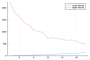
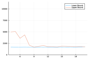
Figure 2 depicts visually the lower and upper bounds on $g$ from Algorithm 2 (left) and after running Algorithm 1 to completion (right) on a synthetic sparse regression instance generated in the fashion described in our numerical experiments, with $\delta\rightarrow+\infty$, $n=200,p=20$, $\gamma=1/\sqrt{n}$, $k_{\text{true}}=10$, $\rho=0.7$, $\nu=1$, where $k\in\{2,\ldots,19\}$, and using the outer-approximation method of Bertsimas and Van Parys (2020) as our solver for each MIO with a time limit of $60$s. We observe that Algorithm 1 solved $1855$ MIOs to identify the optimal $k$, which is a 49% improvement on complete enumeration. In our computational experiments, see Section 5.2, we test Algorithm 1 on real datasets and find that it reduces the number of MIOs that need to be solved by 50-80% with respect to complete enumeration.

Figure 2: Comparison of initial bounds on LOOCV from Algorithm 2 (left) and bounds after running Algorithm 1 (right) for a synthetic sparse regression instance where $p=20,n=200,k_{\text{true}}=10$, for varying $k$.

Minimizing the Confidence-Adjusted LOOCV Error at Scale:

When minimizing $g$ with respect to $k$, Algorithm 1 performs well in settings where $p<1000$, often reducing the number of MIOs that need solving by $70\%$ or more compared to complete enumeration, as we demonstrated in Table 3. Unfortunately, in high-dimensional settings, this is not enough of an improvement over complete enumeration to be numerically tractable, due to the number of MIOs that need solving. Accordingly, in certain settings, we eschew Algorithm 1 and instead use the more tractable saddle-point method of Bertsimas et al. (2020) to estimate $\bm{\beta}_{\text{persp}}^{(i)}$. Notably, this saddle-point method recovers the same regressors as exact methods when $n\gg p$ (see Bertsimas et al. 2020, for precise conditions). Moreover, as we demonstrated in Sections 3.2-3.3, this estimator provides a similar, although slightly different, confidence-adjusted LOOCV error to the MIO, and can therefore be considered a heuristic with the same limiting behavior as Algorithm 1.

4.2 Parametric Optimization of Confidence-Adjusted LOOCV With Respect to $\gamma$

In this section, we propose a technique for approximately minimizing the confidence-adjusted LOOCV error with respect to the regularization hyperparameter $\gamma$.

We begin with two observations from the literature. First, as observed by Stephenson et al. (2021), the LOOCV error $h(\gamma,k)$ is often quasi-convex with respect to $\gamma$ when $k=p$. Second, Bertsimas et al. (2021) reports that, for sparsity-constrained problems, the optimal support often does not change as we vary $\gamma$. Combining these observations suggests that, after optimizing $k$ with $\gamma$ fixed, a good strategy for minimizing $g$ with respect to $\gamma$ is to fix the optimal support $\bm{z}^{(i)}$ with respect to each fold $i$ and invoke a root-finding method to find a $\gamma$ which locally minimizes $g$.

Accordingly, we now use the fact that $\gamma$ and $\bm{z}^{(i)}$ fully determine $\bm{\beta}^{(i)}$ to rewrite

$$\min_{\bm{\beta}\in\mathbb{R}^{p}}\quad \frac{\gamma}{2}\|\bm{\beta}\|_{2}^{2}+\|\bm{X}\bm{\beta}-\bm{y}\|_{2}^{2}\ \text{s.t.}\ \beta_{i}=0\ \text{if}\ \hat{z}_{i}=0,$$

is given by the expression

$$\bm{\beta}^{\star}=\left(\frac{\gamma}{2}\mathbb{I}+\bm{X}^{\top}\mathrm{Diag}(\hat{\bm{z}})\bm{X}\right)^{-1}\mathrm{Diag}(\hat{\bm{z}})\bm{X}^{\top}\bm{y}.$$

Therefore, we fix each $\bm{z}^{(i)}$ and substitute the resulting expressions for each $\bm{\beta}^{(i)}$ into the leave-one-out error, which yields the following univariate optimization problem which can be solved via standard root-finding methods to approximately minimize the confidence-adjusted LOOCV loss in the special case where $\delta\rightarrow+\infty$:

$$\min_{\gamma>0}\sum_{i=1}^{n}\left(y_{i}-\bm{X}_{i}^{\top}\mathrm{Diag}(\bm{z}^{(i)})\left(\frac{\gamma}{2}\mathbb{I}+\bm{X}^{(i)\top}\mathrm{Diag}(\bm{z}^{(i)})\bm{X}^{(i)^{\top}}\right)^{-1}\mathrm{Diag}(\bm{z}^{(i)})\bm{X}^{{(i)}^{\top}}\bm{y}^{(i)}\right)^{2}.$$ (25)

Moreover, if $\delta<\infty$ and we are interested in minimizing the confidence-adjusted LOOCV error, rather than the LOOCV error itself, we assume that the index $j$ at which the expression

$$\mu_{h}:=\max_{j\in[n]}\frac{1}{n}\sum_{j=1}^{n}\left|(y_{i}-{\bm{\beta}^{\star}}^{\top}\bm{x}_{i})^{2}-(y_{i}-\bm{\beta}^{(j)}\bm{x}_{i})^{2}\right|$$

attains its maximum, does not vary as we vary $\gamma$. Fixing $j$ then allows us to derive a similar approximation for the hypothesis stability, namely:

$$\mu_{h}(\gamma,k)\approx\frac{1}{n}\sum_{i\in[n]} \bigg{|}\left(y_{i}-\bm{X}_{i}^{\top}\mathrm{Diag}(\bm{z}^{(j)})\left(\frac{\gamma}{2}\mathbb{I}+\bm{X}^{(j)\top}\mathrm{Diag}(\bm{z}^{(j)})\bm{X}^{(j)^{\top}}\right)^{-1}\mathrm{Diag}(\bm{z}^{(j)})\bm{X}^{{(j)}^{\top}}\bm{y}^{(j)}\right)^{2}$$

$$-\left(y_{i}-\bm{X}_{i}^{\top}\mathrm{Diag}(\bm{z})\left(\frac{\gamma}{2}\mathbb{I}+\bm{X}^{\top}\mathrm{Diag}(\bm{z})\bm{X}^{\top}\right)^{-1}\mathrm{Diag}(\bm{z})\bm{X}^{{}^{\top}}\bm{y}\right)^{2}\bigg{|},$$

where $\bm{z}$ denotes the optimal support when no data observations are omitted. With these expressions, it is straightforward to minimize the confidence-adjusted LOOCV error with respect to $\gamma$.

In our numerical experiments, we find local minimizers of our approximation of $g$ by invoking the ForwardDiff function in Julia to automatically differentiate our approximation of $g$, and subsequently identify local minima via the Order0 method in the Roots.jl package, which is designed to be a robust root-finding method. To avoid convergence to a low-quality local minimum, we run the search algorithm initialized at the previous iterate $\gamma_{t-1}$ and seven points log-uniformly distributed in $[10^{-3},10^{1}]$, and set $\gamma_{t}$ to be the local minima with the smallest estimated error. Moreover, to ensure numerical robustness, we require that $\gamma_{t}$ remains within the bounds $[10^{-3},10^{1}]$ and project $\gamma_{t}$ onto this interval if it exceeds these bounds (this almost never occurs in practice, because the data is preprocessed to be standardized). This approach tends to be very efficient in practice, particularly when the optimal support does not vary significantly as we vary $\gamma$.

5 Numerical Experiments

We now present numerical experiments testing our proposed methods. First, in Section 5.1, we describe the synthetic and real datasets we use throughout our experiments. Then, in Section 5.2, we study the computational savings of using Algorithm 1 over a complete grid search when optimizing the LOOCV error as a function of the sparsity parameter $k$. Then, in Sections 5.3 and 5.4, we use synthetic data to benchmark the statistical performance of the proposed methods (without and with confidence adjustment) against alternatives in the literature. Finally, in Section 5.5, we benchmark the proposed approach on real datasets.

5.1 Datasets

We now describe the datasets we use to test the methods proposed in this paper, and competing alternatives in the literature. We use both synthetically generated data and real data in our experiments. This is because synthetic data allows us to control the ground truth and measure the accuracy of our methods in statistical settings, while real data allows us to measure the performance of our methods on datasets that arise in practice, and ensure that any performance gains with respect to out-of-sample MSE are not an artifice of the data generation process.

5.1.1 Synthetic datasets

We follow the experimental setup in Bertsimas et al. (2020). Given a fixed number of features $p$, number of datapoints $n$, true sparsity $1\leq k_{\text{true}}\leq p$, autocorrelation parameter $0\leq\rho\leq 1$ and signal to noise parameter $\nu$:

1. The rows of the model matrix are generated iid from a $p$-dimensional multivariate Gaussian distribution $\mathcal{N}(\bm{0},\bm{\Sigma})$, where $\Sigma_{ij}=\rho^{|i-j|}$ for all $i,j\in[p]$.

2. A “ground-truth” vector $\bm{\beta}_{\text{true}}$ is sampled with exactly $k_{\text{true}}$ non-zero coefficients. The position of the non-zero entries is randomly chosen from a uniform distribution, and the value of the non-zero entries is either $1$ or $-1$ with equal probability.

3. The response vector is generated as $\bm{y}=\bm{X\beta_{\text{true}}}+\bm{\varepsilon}$, where each $\varepsilon_{i}$ is generated iid from a scaled normal distribution such that $\sqrt{\nu}=\|\bm{X\beta_{\text{true}}}\|_{2}/\|\bm{\varepsilon}\|_{2}$.

4. We standardize $\bm{X},\bm{y}$ to normalize and center them.

5.1.2 Real datasets

We use a variety of real datasets from the literature in our computational experiments. The information of each dataset is summarized in Table 1. Note that we increased the number of features on selected datasets by including second-order interactions.

Dataset	n	p	Notes	Reference
Diabetes	442	11		Efron et al. (2004)
Housing	506	13		Gómez and Prokopyev (2021)
Housing2	506	91	2nd order interactions added	Gómez and Prokopyev (2021)
Wine	6497	11		Cortez et al. (2009)
AutoMPG	392	25		Quinlan (1993)
Hitters	263	19	Removed rows with missing data	Kaggle
			$\bm{y}=\log(\text{salary})$
Prostate	97	8		R Package ncvreg
Servo	167	19	One-hot encoding of features	Ulrich (1993)
Toxicity	38	9		Rousseeuw et al. (2009)
SteamUse	25	8		Rousseeuw et al. (2009)
Alcohol2	44	21	2nd order interactions added	Rousseeuw et al. (2009)
TopGear	242	373		Bottmer et al. (2022)
BarDet	120	200		Ye et al. (2018)
Vessel	180	486		Christidis et al. (2020)
Riboflavin	71	4088		R package hdi

Table 1: Real datasets used.

5.2 Exact Leave-One-Out Optimization

We first assess whether Algorithm 1 significantly reduces the number of MIOs that need to be solved to minimize the LOOCV error with respect to $k$, compared to grid search. For simplicity, we consider the special case where $\delta=\infty$, giving the bilevel optimization problem:

$$\min_{k\in[p],\{\bm{\beta}^{(i)}\}_{i=1}^{n}}\; \sum_{i=1}^{n}(y_{i}-\bm{x_{i}}^{\top}\bm{\beta}^{(i)})^{2}$$ (26a)

s.t. $$\bm{\beta}^{(i)}\in\arg\min_{\bm{\beta}\in\mathbb{R}^{p}:\ \|\bm{\beta}\|_{0}\leq k}\ \frac{\gamma}{2}\|\bm{\beta}\|_{2}^{2}+\|\bm{X}^{(i)}\bm{\beta}-\bm{y}^{(i)}\|_{2}^{2}\quad\forall i\in[n].$$ (26b)

We compare the performance of two approaches. First, a standard grid search approach (Grid), where we solve the inner MIO (26b) for all combinations of cardinality $k\in[p]$ and all folds of the data $i\in[n]$, and select the hyperparameter combination which minimizes (26a). To ensure the quality of the resulting solution, we solve all MIOs to optimality (without any time limit). Second, we consider using Algorithm 1 with parameter $r=\infty$ (thus solving MIOs to optimality until the desired optimality gap $\epsilon$ for problem (26) is proven). We test regularization parameter $\gamma\in\{0.01,0.02,0.05,0.10,0.20,0.50,1.00\}$, set $\delta=\infty$, $r=\infty$ and $\epsilon=0.01$ in Algorithm 1, and solve all MIOs via their perspective reformulations, namely

$$\min_{\bm{\beta}\in\mathbb{R}^{p},\bm{z}\in\{0,1\}^{p}}\; \|\bm{X}\bm{\beta}-\bm{y}\|_{2}^{2}+\frac{\gamma}{2}\sum_{j=1}^{p}\frac{\beta_{j}^{2}}{z_{j}}\ \text{s.t.}\ \sum_{j=1}^{p}z_{j}\leq k,$$

using Mosek 10.0. Since running the approach Grid involves solving $\mathcal{O}(np)$ MIOs (without a time limit), we are limited to testing these approaches on small datasets, and accordingly use the Diabetes, Housing, Servo, and AutoMPG datasets for this experiment. Moreover, we remark that the specific solution times and the number of nodes expanded by each method are not crucial, as those could vary substantially if relaxations other than the perspective are used, a different solvers or solution approach is used, or if advanced techniques are implemented (but both methods would be affected in the same way). Thus, we focus our analysis on relative performance.

We now summarize our experimental results and defer the details to Table 5 of Appendix 9. Figure 3 summarizes the percentage reduction of the number of MIOs and the number of branch-and-bound nodes achieved by Algorithm 1 over Grid, computed as

$$\text{Reduction in MIOs}=\frac{\text{\# MIO}_{\texttt{Grid}}-\text{\# MIO}_{\text{Alg.\ref{alg:parametricK}}}}{\text{\# MIO}_{\texttt{Grid}}},\;\;\text{Reduction in nodes}=\frac{\text{\# nodes}_{\texttt{Grid}}-\text{\# nodes}_{\text{Alg.\ref{alg:parametricK}}}}{\text{\# nodes}_{\texttt{Grid}}},$$

where $\text{\# MIO}_{\text{Y}}$ and $\text{\# nodes}_{\text{Y}}$ indicate the number of MIOs or nodes used by method Y.

Figure 3: Reduction in the number of MIO solved (left) and the total number of branch-and-bound nodes (right) when using Algorithm 1, when compared with Grid (i.e., independently solving $\mathcal{O}(pn)$ MIOs) in four real datasets. The distributions shown in the figure correspond to solving the same instance with different values of $\gamma$. All MIOs are solved to optimality, without imposing any time limits.

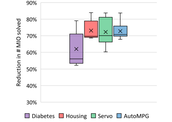
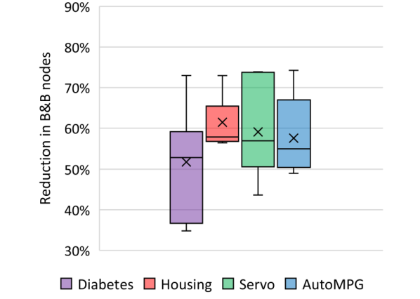
We observe that across these four datasets, Algorithm 1 reduces the number of MIO that need to be solved by 70%, on average, and the overall number of branch-and-bound nodes by 57%, on average (the reduction in computational times is similar to the reduction of nodes). These results indicate that the relaxations of the bilevel optimization (21) derived in §3 are sufficiently strong to avoid solving most of the MIOs that traditional methods such as Grid would solve, without sacrificing solution quality. The resulting approach still requires solving several MIOs but, as we show throughout the rest of this section, approximating each MIO with its perspective relaxation yields similarly high quality statistical estimators at a fraction of the computational cost.

5.3 Sparse Regression on Synthetic Data

We now benchmark our coordinate descent approach (without any confidence adjustment) on synthetic sparse regression problems where the ground truth is known to be sparse, but the number of non-zeros is unknown. The goal of this experiment is to highlight the dangers of cross-validating without a confidence adjustment procedure.

We consider two problem settings. First, a smaller-scale setting $(p=50,k_{\text{true}}=10)$ that allows us to benchmark two implementations of our coordinate descent approach:

1. An exact implementation of our approach, where we optimize $k$ according to Algorithm 1, using Gurobi version $9.5.1$ to solve all MIOs with a time limit of $120$s, and warm-start Gurobi with a greedily rounded solution to each MIO’s perspective relaxation (computed using Mosek version $10.0$) before running Gurobi. We denote this approach by “EX” (stands for EXact).

2. An approximate implementation of our approach, where we optimize $k$ by greedily rounding the perspective relaxation of each MIO we encounter (computed using Mosek version $10.0$), and using these greedily rounded solutions, rather than optimal solutions to MIOs, to optimize the leave-one-out error with respect to $k$. We denote this approach by “GD” (stands for GreeDy).

For both approaches, we optimize $\gamma$ as described in Section 4.2, and set $k_{\min}=4,k_{\max}=20$.

We also consider a large-scale setting $(p=1000,k_{\text{true}}=20)$ where grid search techniques are not sufficient to identify globally optimal solutions with respect to the LOOCV loss. In this setting, the subproblems are too numerically expensive to solve exactly, and accordingly, we optimize $k$ using an approach very similar to “GD”, except to optimize $k$ we solve each subproblem using the saddle-point method of Bertsimas et al. (2020) with default parameters, rather than greedily rounding the perspective relaxations of MIOs. This approach generates solutions that are almost identical to those generated by GD, but is more scalable. We term this implementation of our coordinate descent approach “SP” (stands for Saddle Point), and set $k_{\min}=10,k_{\max}=40$ when optimizing $k$ in this experiment.

We compare against the following state-of-the-art methods, using in-built functions to approximately minimizes the cross-validation loss with respect to the method’s hyperparameters via grid search, and subsequently fit a regression model on the entire dataset with these cross-validated parameters (see also Bertsimas et al. (2020) for a detailed discussion of these approaches):

• The ElasticNet method in the ubiquitous GLMNet package, with grid search on their parameter $\alpha\in\{0,0.1,0.2,\ldots,1\}$, using $100$-fold cross-validation as in (Bertsimas et al. 2020).

• The Minimax Concave Penalty (MCP) and Smoothly Clipped Absolute Deviation Penalty (SCAD) as implemented in the R package ncvreg, using the cv.ncvreg function with $100$ folds and default parameters to (approximately) minimize the cross-validation error.

• The L0Learn.cvfit method implemented in the L0Learn R package (c.f. Hazimeh and Mazumder 2020), with $n$ folds, a grid of $10$ different values of $\gamma$ and default parameters otherwise.

We remark that using cv.GLMNet and cv.ncvreg functions to minimize the LOOCV is orders-of-magnitude more expensive than other approaches, thus we settle with minimizing $100$-fold cross-validation error as a surrogate.

Experimental Methodology:

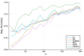
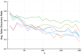
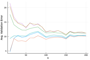
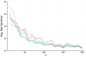
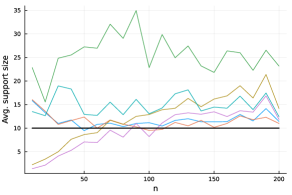
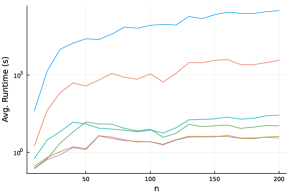
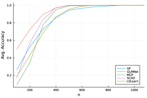
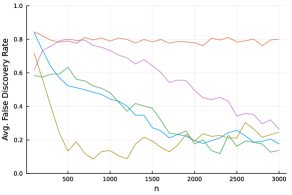
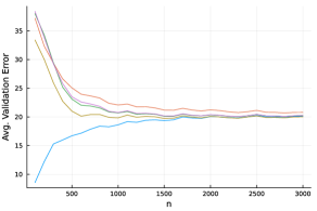
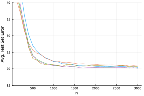
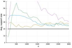
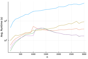
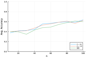
We measure each method’s ability to recover the ground truth (true positive rate) while avoiding detecting irrelevant features (false discovery rate). We consider two sets of synthetic data, following Bertsimas et al. (2020): a small (medium noise, high correlation) dataset: $k_{\text{true}}=10$, $p=50$, $\rho=0.7$ and $\nu=1$; and a large (medium noise, low correlation) dataset: $k_{\text{true}}=20$, $p=1000$, $\rho=0.2$ and $\nu=1$. Figure 4 reports results in small instances with varying number of samples $n\in\{10,20,\ldots,200\}$, and Figure 5 reports results for large datasets with $n\in\{100,200,\ldots,3000\}$. We report the average cross-validated support size, average overall runtime, average leave-one-out error, and average MSE on a different (out-of-sample) set of $10000$ observations of $\bm{X},\bm{y}$ drawn from the same distribution.

Figure 4: Average accuracy (top left), false discovery rate (top right), normalized validation error (middle left), normalized MSE on test set (middle right), cross-validated support (bottom left) and runtime (bottom right) as $n$ increases with $p=50,k_{\text{true}}=10$, for coordinate descent with $k$ optimized using Algorithm 1 (EX), coordinate descent with $k$ optimized by greedily rounding perspective relaxations (GD), GLMNet, MCP, SCAD, and L0Learn. We average results over $25$ datasets.

Figure 5: Average accuracy (top left), false discovery rate (top right), normalized validation error (middle left), normalized MSE on test set (middle right), cross-validated support (bottom left) and runtime (bottom right) as $n$ increases with $p=1000,k_{\text{true}}=20$, for coordinate descent with a saddle-point method to solve each training problem when optimizing $k$ (SP), GLMNet, MCP, SCAD, and L0Learn. We average results over $25$ datasets.

Accuracy and Performance of Methods:

We observe that our coordinate descent schemes and L0Learn consistently provide the best performance in large-sample settings, by returning sparser solutions with a lower false discovery rate and a similar out-of-sample MSE to all other methods when $n>p$. On the other hand, GLMNet appears to perform best when $n\ll p$, where it consistently returns solutions with a lower out-of-sample MSE and less out-of-sample disappointment than any other method. Thus, the best-performing methods varies depends on the number of samples, as recently suggested by a number of authors (Hastie et al. 2020, Bertsimas and Van Parys 2020).

Out-of-Sample Disappointment:

We observe that all methods suffer from the optimizer’s curse (c.f. Smith and Winkler 2006, Van Parys et al. 2021), with the average MSE on the test set being consistently larger than the average leave-one-out error on the validation set, especially when $n$ is smaller. However, out-of-sample disappointment is most pronounced for our coordinate descent schemes and L0Learn, which consistently exhibit the lowest LOOCV error at all sample sizes but the highest test set error in small-data settings. As reflected in the introduction, this phenomenon can be explained by the fact that optimizing the leave-one-out cross-validation error without any confidence adjustment generates highly optimistic estimates of the corresponding test set error. This reinforces the need for confidence-adjusted alternatives to the leave-one-out error, particularly in small-sample settings, and motivates the confidence-adjusted variants of our coordinate descent scheme we study in the next section.

5.4 Confidence-Adjusted Sparse Regression on Synthetic Data

We now benchmark our coordinate descent schemes with confidence adjustment. In particular, we revisit the problem settings studied in the previous section, and consider setting $\delta=0.1$ and $\delta=1$ in our GD and SP implementations of coordinate descent. Specifically, we solve each subproblem using greedy rounding when $p=50,k_{\text{true}}=10$ and via a saddle-point method when $p=1000,k_{\text{true}}=20$. For ease of comparison, we also report the performance of these inexact methods without any confidence adjustment, as reported in the previous section.

Experimental Methodology:

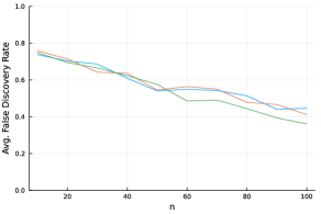
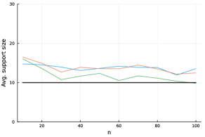
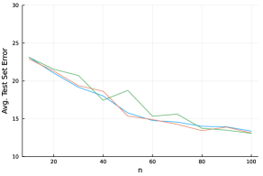
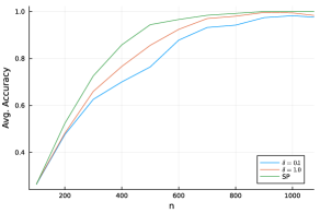
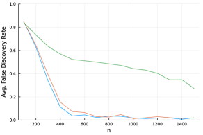
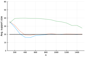
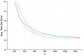
We implement the same methodology as in the previous section, and vary $n\in\{10,20,\ldots,100\}$ for small instances (Figure 6) and $n\in\{100,200,\ldots,1500\}$ for large instances (Figure 7). We report the average accuracy, average false positive rate, average cross-validated support size and average MSE on a different (out-of-sample) set of $10000$ observations of $\bm{X},\bm{y}$ drawn from the same distribution.

Figure 6: Average accuracy (top left), false discovery rate (top right), cross-validated support (bottom left), and normalized MSE on test set (bottom right) as $n$ increases with $p=50,k_{\text{true}}=10$, for coordinate descent with confidence adjustment with $\delta\in\{0.1,1.0\}$, and without any confidence adjustment (GD). We average results over $25$ datasets.

Figure 7: Average accuracy (top left), false discovery rate (top right), cross-validated support (bottom left), and normalized MSE on test set (bottom right) as $n$ increases with $p=1000,k_{\text{true}}=20$, for coordinate descent with confidence adjustment and $\delta\in\{0.1,1.0\}$, and without any confidence adjustment (SP). We use a saddle-point method to approximately solve all sparse regression subproblems for all methods, and average results over $25$ datasets.

Impact of Confidence Adjustment on Test Set Performance:

We observe that for both problem settings, accounting for out-of-sample disappointment via confidence adjustment significantly improves the test set performance of sparse regression methods with hyperparameters selected via cross-validation. On average, we observe a $2.55\%$ (resp. $3.04\%$) average MSE improvement for $\delta=0.1$ (resp. $\delta=1.0$) when $p=50$, and a $2.75\%$ (resp. $5.48\%$) average MSE improvement for $\delta=0.1$ (resp. $\delta=1.0$) when $p=1000$, with the most significant out-of-sample performance gains occurring when $n$ is smallest. This performance improvement highlights the benefits of accounting for out-of-sample disappointment by selecting more stable sparse regression models, and suggests that accounting for model stability when cross-validating is a viable alternative to selecting hyperparameters that minimize the leave-one-out error that often yields better test-set performance.

We further observe that when $p=1000$, accounting for model stability via confidence adjustment produces sparser regressors with a significantly lower false discovery rate ($5\%$ vs. $40\%$ when $n=1000$), which suggests that models selected via a confidence adjustment procedure may sometimes be less likely to select irrelevant features. However, we caution that when $p=50$, the models selected via a confidence-adjusted procedure exhibit a similar false discovery rate to models selected by minimizing the LOOCV error, so this effect does not appear to occur uniformly.

All-in-all, the best value of $\delta$ to select for a confidence adjustment procedure appears to depend on the amount of data available, with smaller values like $\delta=0.1$ performing better when $n$ is small, but being overly conservative when $n$ is large, and larger values like $\delta=1.0$ providing a less significant benefit when $n$ is very small but performing more consistently when $n$ is large.

5.5 Benchmarking on Real-World Datasets

We now benchmark our proposed cross-validation approaches against the methods studied in the previous section on a suite of real-world datasets previously studied in the literature. For each dataset, we repeat the following procedure five times: we randomly split the data into $80\%$ training/validation data and $20\%$ testing data, and report the average sparsity of the cross-validated model and the average test-set MSE.

Table 2 depicts the dimensionality of each dataset, the average cross-validation error (“CV”), the average test-set error (“MSE”), and the sparsity attained by our cyclic coordinate descent without any confidence adjustment (“SP”), our cyclic coordinate descent with $\delta=1.0$ (“$\delta=1.0$”), MCP, and GLMNet on each dataset. We used the same number of folds for MCP and GLMNet as in the previous section, i.e., a cap of $100$ folds, for the sake of numerical tractability. Note that for our coordinate descent methods, after identifying the final hyperparameter combination $(\gamma,k)$ we solve a MISOCP with a time limit of $3600$s to fit a final model to the training dataset. Moreover, for our cyclic coordinate descent schemes, we set the largest permissible value of $k$ such that $k\log k\leq n$ via the Lambert.jl Julia package, because Gamarnik and Zadik (2022, Theorem 2.5) demonstrated that, up to constant terms and under certain assumptions on the data generation process, on the order of $k\log k$ observations are necessary to recover a sparse model.

Dataset	n	p	SP			$\delta=1.0$			MCP			GLMNet
			$k$	CV	MSE	$k$	CV	MSE	$k$	CV	MSE	$k$	CV	MSE
Wine	6497	11	10	0.434	0.543	2	0.809	0.709	10.6	0.434	0.543	11	0.434	0.543
Auto-MPG	392	25	16.4	6.731	8.952	11.4	45.44	13.10	15	7.066	8.983	18.8	7.072	8.839
Hitters	263	19	7.4	0.059	0.080	4.6	0.169	0.095	12.4	0.062	0.080	13	0.062	0.080
Prostate	97	8	4.4	0.411	0.590	2.6	1.825	0.632	6.8	0.439	0.566	6.8	0.435	0.574
Servo	167	19	9.2	0.537	0.812	3.6	4.094	1.095	11.6	0.565	0.729	15.4	0.568	0.717
Housing2	506	91	56.4	10.32	13.99	65.6	79.33	16.37	31.2	12.93	15.54	86.4	9.677	11.52
Toxicity	38	9	3.2	0.031	0.057	2.8	0.249	0.064	3	0.033	0.061	4.2	0.035	0.061
SteamUse	25	8	3	0.346	0.471	2.6	2.948	0.769	2.4	0.441	0.506	4.2	0.458	0.507
Alcohol2	44	21	3	0.186	0.254	5.6	13.79	0.304	2	0.185	0.232	4.4	0.212	0.260
TopGear	242	373	18	0.032	0.053	11.6	0.482	0.072	8.2	0.040	0.069	24.6	0.036	0.053
BarDet	120	200	19.6	0.005	0.011	18	0.107	0.011	6	0.006	0.010	61	0.006	0.009
Vessel	180	486	21	0.014	0.031	28.6	2.272	0.025	2.6	0.028	0.033	53.2	0.015	0.022
Riboflavin	71	4088	18	0.055	0.304	14.6	1.316	0.443	9.2	0.277	0.232	82.8	0.164	0.279

Table 2: Average performance of methods across a suite of real-world datasets where the ground truth is unknown (and may not be sparse), sorted by how overdetermined the dataset is ($n/p$), and separated into the underdetermined and overdetermined cases. In overdetermined settings, cyclic coordinate descent (without confidence) returns sparser solutions than MCP or GLMNet and maintains a comparable average MSE. In underdetermined settings, cyclic coordinate descent with confidence returns significantly sparse solutions than GLMNet with a comparable MSE, and more accurate (although denser) solutions than MCP.

We observe that our cyclic coordinate scheme without confidence adjustment returns solutions with a significantly lower cross-validation error than all other methods. Specifically, our LOOCV error is $34.2\%$ lower than GLMNet’s and $48.5\%$ lower than MCP’s on average. Moreover, our methods obtain significantly sparser solutions than GLMNet (SP is $37.9\%$ sparser than GLMNet, $\delta=1.0$ is $49.6\%$ sparser than GLMNet, MCP is $44.1\%$ sparser than GLMNet, on average).

However, this does not result in a lower test set error on most datasets (SP is $6.35\%$ higher, $\delta=1.0$ is $30.49\%$ higher, MCP is $6.82\%$ higher, on average), because, as discussed previously, optimizing the cross-validation error increases the cyclic coordinate descent scheme’s vulnerability to out-of-sample disappointment, due to the optimizer’s curse (Smith and Winkler 2006). In the case of confidence-adjusted coordinate descent, this can be explained by the fact that $\delta=1.0$ causes the method to be excessively risk-averse in some settings, and a larger value of $\delta$ may actually be more appropriate. In particular, calibrating $\delta\in\mathbb{R}_{++}$ to match the cross-validation error of GLMNet or MCP may be a better strategy for obtaining high-quality solutions that do not disappoint significantly out-of-sample and are not too risk averse.

Motivated by these observations, we now rerun our cyclic coordinate descent scheme with $\delta\in\{10,100,1000,\ldots,10^{7}\}$. Tables 3-4 depicts the average validation and test set error from these variants of our cyclic coordinate descent scheme, and verifies that, in circumstances where $\delta=1$ led to an excessively conservative validation error, a larger value of $\delta$ performs better on the test set. We also report the sparsity and MSE for the values of $\delta$ such that the confidence-adjusted LOOCV error most closely matches the cross-validation error reported by GLMNet.

Dataset	n	p	$\delta=10$			$\delta=100$			$\delta=1000$			$\delta=10000$
			$k$	CV	MSE	$k$	CV	MSE	$k$	CV	MSE	$k$	CV	MSE
Wine	6497	11	2	0.642	0.565	3.6	0.587	0.682	10	0.560	0.543	10	0.548	0.565
Auto-MPG	392	25	18.6	20.43	9.206	18	12.23	8.867	17.8	9.638	8.854	17.8	8.857	8.881
Hitters	263	19	7.2	0.108	0.085	7.2	0.085	0.081	7.2	0.078	0.080	7.2	0.075	0.080
Prostate	97	8	2.8	0.941	0.600	3	0.653	0.598	3.6	0.560	0.563	4.4	0.529	0.590
Servo	167	19	10	1.817	0.761	10.2	1.049	0.771	10.2	0.798	0.775	9.8	0.715	0.729
Housing2	506	91	78.4	32.91	11.65	77.2	18.01	11.31	62.2	15.887	14.218	57.8	13.795	16.021
Toxicity	38	9	3	0.1	0.061	3	0.057	0.060	3.2	0.045	0.057	3.2	0.040	0.057
SteamUse	25	8	4.6	1.268	0.597	3.4	0.729	0.589	3.4	0.536	0.653	3.4	0.484	0.662
Alcohol2	44	21	4.6	4.521	0.289	4.6	1.594	0.296	2	0.674	0.213	2	0.360	0.218
TopGear	242	373	10.4	0.211	0.073	28.4	0.115	0.062	40.4	0.066	0.057	26.6	0.050	0.053
Bardet	120	200	23	0.033	0.011	22	0.015	0.011	20.4	0.010	0.009	19	0.007	0.013
Vessel	180	486	32.2	0.731	0.026	25.8	0.317	0.028	23.8	0.114	0.028	16.8	0.048	0.030
Riboflavin	71	4088	18.2	0.469	0.272	18.2	0.194	0.259	18.6	0.105	0.303	18.6	0.076	0.379

Table 3: Performance of methods across real-world datasets where the ground truth is unknown (continued).

Dataset	n	p	$\delta=10^{5}$			$\delta=10^{6}$			$\delta=10^{7}$			$\delta$ calibrated
			$k$	CV	MSE	$k$	CV	MSE	$k$	CV	MSE	$\delta$	$k$	MSE
Wine	6497	11	10	0.544	0.543	10	0.543	0.543	10	0.542	0.565	$10^{7}$	10	0.565
Auto-MPG	392	25	17.2	8.561	8.880	16.6	8.473	8.859	16.8	8.441	8.893	$10^{7}$	16.8	8.893
Hitters	263	19	5.8	0.075	0.080	8.8	0.074	0.080	8.6	0.074	0.080	$10^{7}$	8.6	0.080
Prostate	97	8	4.4	0.518	0.590	4.4	0.515	0.590	4.4	0.514	0.590	$10^{7}$	4.4	0.590
Servo	167	19	10	0.690	0.725	9.4	0.678	0.816	9.8	0.672	0.725	$10^{7}$	9.8	0.725
Housing2	506	91	60	12.496	13.310	64.4	11.029	11.337	55.4	12.547	13.154	$10^{6}$	64.4	11.337
Toxicity	38	9	3.2	0.039	0.057	3.2	0.038	0.057	3.2	0.038	0.057	$10^{7}$	3.2	0.057
SteamUse	25	8	3.4	0.466	0.652	3.4	0.460	0.652	3.4	0.458	0.662	$10^{7}$	3.4	0.662
Alcohol2	44	21	2	0.256	0.230	2	0.227	0.230	2	0.217	0.230	$10^{7}$	2	0.230
TopGear	242	373	24.6	0.043	0.053	29.2	0.041	0.053	26.2	0.040	0.053	$10^{7}$	26.2	0.053
Bardet	120	200	14.4	0.007	0.011	19.6	0.007	0.010	21.4	0.006	0.010	$10^{7}$	21.4	$0.010$
Vessel	180	486	16.4	0.030	0.027	15	0.023	0.030	16	0.019	0.026	$10^{7}$	16	0.026
Riboflavin	71	4088	18.8	0.071	0.288	17.2	0.072	0.282	18.4	0.065	0.316	100	18.2	0.259

Table 4: Performance of methods across real-world datasets where the ground truth is unknown (continued).

We observe that, after normalizing all metrics against the metric obtained by GLMNet on the same dataset to weigh all datasets equally, the average relative MSE from cyclic coordinate descent with confidence adjustment (calibrated) is $2.62\%$ higher than GLMNet, and the average regressor is $33.6\%$ sparser than GLMNet. This compares favorably with our previous results with $\delta=1,\delta\rightarrow+\infty$ and MCP, because it corresponds to an MSE improvement of $4\%$ out-of-sample without compromising the sparsity of our regressors.

6 Conclusion

In this paper, we propose a new approach for selecting hyperparameters in ridge-regularized sparse regression problems, minimizing a generalization bound on the test-set performance. By leveraging perspective relaxations and branch-and-bound techniques from mixed-integer optimization, we minimize the bound by performing alternating minimization on a sparsity hyperparameter and a regularization hyperparameter. Our approach obtains locally optimal hyperparameter combinations with $p=1000$ features in hours, and thus is a viable hyperparameter selection technique in offline settings where sparse and stable regressors are desirable. Empirically, we observe that, in underdetermined settings, our approach improves the out-of-sample MSE by $2\%$–$7\%$ compared to approximately minimizing the leave-one-out error, which suggests that model stability and performance on a validation metric should both be accounted for when selecting regression models.

Future work could involve exploring the benefits of minimizing generalization bounds, rather than leave-one-out or $k$-fold metrics, when hyperparameter tuning in other problem settings with limited amounts of data. It would also be interesting to investigate whether tighter convex relaxations of sparse regression than the perspective relaxation could be used to develop tighter bounds on the prediction spread and the hypothesis stability.

Acknowledgements:

Andrés Gómez is supported in part by grant 2152777 from the National Science Foundation and grant FA9550-22-1-0369 from the Air Force Office of Scientific Research.

Endnotes

1. 1 This assumption is not entirely unreasonable since the training objective is strongly convex for a fixed binary support vector, and therefore for each binary support vector there is indeed a unique solution. One could relax this assumption by defining $h(\gamma,k)$ to be the minimum leave-one-out error over all training-optimal solutions $\bm{\beta}^{(i)}$, as is commonly done in the bilevel optimization literature, giving what is called an optimistic formulation of a bilevel problem (see Beck and Schmidt 2021, for a review). However, this would make the leave-one-out error less tractable.
2. 2 We remark that applying this bias correction term is equivalent to normalizing the least squares error $\|\bm{X}\bm{\beta}-\bm{Y}\|_{2}^{2}$ in the training problem, by dividing this term by the number of data points $n$ (or $n-1$).
3. 3 Throughout this paper, for the sake of simplicity, we follow Bousquet and Elisseeff (2002) in deliberately not providing a precise definition of bias and variance, and instead resort to common intuition about these concepts.
4. 4 Note that requiring that a trace is non-negative is less stringent than requiring a matrix is positive semidefinite, and multiplying both sides of a PSD constraint by $\bm{W}$ could make the PSD constraint less stringent.
5. 5 We omit some details around bounding the hypothesis stability for the sake of brevity; these bounds can be obtained in much the same way as the bounds on the LOOCV error, with a minor implementation detail around whether to compute $\bm{\beta}(k)$, an optimal regressor with no data points left out and a sparsity constraint of $k$, before or after running the method; the method performs well in either case.
6. 6 We remark that one could also generate a grid of allowable values of $\gamma$ and proceed in the same manner as in the previous section, although this would be less numerically tractable and may not even generate locally optimal $\gamma$’s.
7. 7 We pick the first index $j$ which attains this maximum in the rate case of ties.
8. 8 We remark that the cross-validation error when $\delta$ is very large does not always appear to converge to the cross-validation error without confidence adjustment. This can be explained by the fact that owing to the $1/\sqrt{n}$ term in the confidence adjustment term and the $1/n$ term in the LOOCV error, even larger values of $\delta$ may be needed to observe the behavior of the LOOCV error as $\delta\rightarrow\infty$, and that the presence of the confidence adjustment term means that our root finding method may identify a different local minimum in some cases.

Supplementary Material

7 Omitted Proofs

7.1 Proof of Theorem 3.1

Proof 7.1

Proof of Theorem 3.1 Consider the problem

$$u=\min_{\bm{\beta}\in\mathbb{R}^{p}} \|\bm{X}\bm{\beta}-\bm{y}\|_{2}^{2}+\frac{\gamma}{2}\|\bm{\beta}\|_{2}^{2}\ \text{s.t.}\ \|\bm{\beta}\|_{0}\leq k$$ (27)

and, given any $0<2\epsilon<\gamma$ and $\bm{x}\in\mathbb{R}^{p}\setminus\bm{0}$, consider the following perspective reformulation parametrized by $\xi\in\mathbb{R}$

$$\phi(\xi)=\min_{\bm{\beta}\in\mathbb{R}^{p},\bm{z}\in[0,1]^{p}}\; \|\bm{X}\bm{\beta}-\bm{y}\|_{2}^{2}+\epsilon\|\bm{\beta}\|_{2}^{2}+\frac{\gamma-2\epsilon}{2}\sum_{j=1}^{p}\frac{\beta_{j}^{2}}{z_{j}}\ \text{s.t.}\ \sum_{j=1}^{p}z_{j}\leq k,\ \bm{x^{\top}\beta}=\xi.$$

Given any upper bound $\bar{u}\geq u$ and lower bound $\underline{\phi}(\xi)\leq\phi(\xi)$, if $\underline{\phi}(\xi)>\bar{u}$ we know setting $\bm{x^{\top}\beta}=\xi$ is not possible in any optimal solution of (27), and we say value $\xi$ is not admissible. Our goal is to establish an interval $[\underline{\xi},\bar{\xi}]$ so that all values outside this interval are not admissible.

First, using arguments identical to Atamtürk and Gómez (2020), observe that

$$\phi(\xi)=\max_{\bm{w}\in\mathbb{R}^{p}}\min_{\bm{\beta}\in\mathbb{R}^{p},\bm{z}\in[0,1]^{p}}\; \|\bm{X}\bm{\beta}-\bm{y}\|_{2}^{2}+\epsilon\|\bm{\beta}\|_{2}^{2}+\frac{\gamma-2\epsilon}{2}\sum_{j=1}^{p}\left(w_{j}\beta_{j}-\frac{w_{j}^{2}}{4}z_{j}\right)$$

s.t. $$\sum_{j=1}^{p}z_{j}\leq k,\ \bm{x^{\top}\beta}=\xi.$$

Moreover, by considering the Lagrangian relaxation with respect to constraint $\bm{x^{\top}\beta}=\xi$, we find

$$\phi(\xi)=\max_{\bm{w}\in\mathbb{R}^{p},\lambda\in\mathbb{R}}\min_{\bm{\beta}\in\mathbb{R}^{p},\bm{z}\in[0,1]^{p}}\; \|\bm{X}\bm{\beta}-\bm{y}\|_{2}^{2}+\epsilon\|\bm{\beta}\|_{2}^{2}+\frac{\gamma-2\epsilon}{2}\sum_{j=1}^{p}\left(w_{j}\beta_{j}-\frac{w_{j}^{2}}{4}z_{j}\right)-\lambda\xi+\lambda(\bm{x^{\top}\beta})$$

s.t. $$\sum_{j=1}^{p}z_{j}\leq k.$$

In any optimal solution of the inner minimization problem, we find that

$$0 =2(\bm{X}^{\top}\bm{X}+\epsilon\mathbb{I})\bm{\beta}-2\bm{X}^{\top}\bm{y}+\frac{\gamma-2\epsilon}{2}\bm{w}+\lambda\bm{x}$$

$$\Leftrightarrow\bm{\beta^{*}} =\left(\bm{X}^{\top}\bm{X}+\epsilon\mathbb{I}\right)^{-1}\left(\bm{X}^{\top}\bm{y}-\frac{\gamma-2\epsilon}{4}\bm{w}-\frac{\lambda}{2}\bm{x}\right).$$

Moreover, we also find that $z_{j}^{*}=1$ for the largest $k$ values of $w_{j}^{2}$ and $z_{j}^{*}=0$ otherwise – we use $\sum_{j=1}^{k}w_{[j]}^{2}$ to denote $\sum_{j=1}^{p}w_{j}^{2}z_{j}^{*}$. Finally, the optimal value of $\lambda$ is such that

$$\xi=\bm{x^{\top}\beta^{*}}\ \Leftrightarrow\;\xi=\bm{x}^{\top}\left(\bm{X}^{\top}\bm{X}+\epsilon\mathbb{I}\right)^{-1}\left(\bm{X}^{\top}\bm{y}-\frac{\gamma-2\epsilon}{4}\bm{w}-\frac{\lambda}{2}\bm{x}\right)$$

$$\Leftrightarrow\; \frac{\lambda}{2}\bm{x}^{\top}\left(\bm{X}^{\top}\bm{X}+\epsilon\mathbb{I}\right)^{-1}\bm{x}=\bm{x}^{\top}\left(\bm{X}^{\top}\bm{X}+\epsilon\mathbb{I}\right)^{-1}\left(\bm{X}^{\top}\bm{y}-\frac{\gamma-2\epsilon}{4}\bm{w}\right)-\xi$$

$$\implies\; \lambda^{*}=2\frac{\bm{x}^{\top}\left(\bm{X}^{\top}\bm{X}+\epsilon\mathbb{I}\right)^{-1}\left(\bm{X}^{\top}\bm{y}-\frac{\gamma-2\epsilon}{4}\bm{w}\right)-\xi}{\bm{x}^{\top}\left(\bm{X}^{\top}\bm{X}+\epsilon\mathbb{I}\right)^{-1}\bm{x}},$$

where the last inequality assumes that $\bm{x}^{\top}\left(\bm{X}^{\top}\bm{X}+\epsilon\mathbb{I}\right)^{-1}\bm{x}\neq 0$, which holds since $\bm{x}\neq\bm{0}$ and $\bm{X}^{\top}\bm{X}+\epsilon\mathbb{I}\succ 0$. We now compute a closed form expression of $\phi(\xi)$ by replacing the quantities $(\lambda,\bm{\beta},\bm{z})$ with their optimal values:

$$\phi(\xi)= \|\bm{y}\|_{2}^{2}+\max_{\bm{w}\in\mathbb{R}^{p},\lambda\in\mathbb{R}}-\lambda\xi$$

$$-\left(\bm{X}^{\top}\bm{y}-\frac{\gamma-2\epsilon}{4}\bm{w}-\frac{\lambda}{2}\bm{x}\right)^{\top}\left(\bm{X}^{\top}\bm{X}+\epsilon\mathbb{I}\right)^{-1}\left(\bm{X}^{\top}\bm{y}-\frac{\gamma-2\epsilon}{4}\bm{w}-\frac{\lambda}{2}\bm{x}\right)-\frac{\gamma-2\epsilon}{8}\sum_{j=1}^{k}w_{[j]}^{2}$$

$$\Leftrightarrow\;\phi(\xi)= \|\bm{y}\|_{2}^{2}+\max_{\bm{w}\in\mathbb{R}^{p},\lambda\in\mathbb{R}}-\left(\bm{X}^{\top}\bm{y}-\frac{\gamma-2\epsilon}{4}\bm{w}\right)^{\top}\left(\bm{X}^{\top}\bm{X}+\epsilon\mathbb{I}\right)^{-1}\left(\bm{X}^{\top}\bm{y}-\frac{\gamma-2\epsilon}{4}\bm{w}\right)-\frac{\gamma-2\epsilon}{8}\sum_{j=1}^{k}w_{[j]}^{2}$$

$$-\frac{\lambda^{2}}{4}\bm{x^{\top}}\left(\bm{X}^{\top}\bm{X}+\epsilon\mathbb{I}\right)^{-1}\bm{x}+\lambda\left(\bm{X}^{\top}\bm{y}-\frac{\gamma-2\epsilon}{4}\bm{w}\right)^{\top}\left(\bm{X}^{\top}\bm{X}+\epsilon\mathbb{I}\right)^{-1}\bm{x}-\lambda\xi$$

$$\Leftrightarrow\;\phi(\xi)= \|\bm{y}\|_{2}^{2}+\max_{\bm{w}\in\mathbb{R}^{p}}-\left(\bm{X}^{\top}\bm{y}-\frac{\gamma-2\epsilon}{4}\bm{w}\right)^{\top}\left(\bm{X}^{\top}\bm{X}+\epsilon\mathbb{I}\right)^{-1}\left(\bm{X}^{\top}\bm{y}-\frac{\gamma-2\epsilon}{4}\bm{w}\right)-\frac{\gamma-2\epsilon}{8}\sum_{j=1}^{k}w_{[j]}^{2}$$

$$-\frac{\left(\bm{x}^{\top}\left(\bm{X}^{\top}\bm{X}+\epsilon\mathbb{I}\right)^{-1}\left(\bm{X}^{\top}\bm{y}-\frac{\gamma-2\epsilon}{4}\bm{w}\right)-\xi\right)^{2}}{\bm{x^{\top}}\left(\bm{X}^{\top}\bm{X}+\epsilon\mathbb{I}\right)^{-1}\bm{x}}$$

$$+2\frac{\bm{x}^{\top}\left(\bm{X}^{\top}\bm{X}+\epsilon\mathbb{I}\right)^{-1}\left(\bm{X}^{\top}\bm{y}-\frac{\gamma-2\epsilon}{4}\bm{w}\right)\left(\bm{X}^{\top}\bm{y}-\frac{\gamma-2\epsilon}{4}\bm{w}\right)^{\top}\left(\bm{X}^{\top}\bm{X}+\epsilon\mathbb{I}\right)^{-1}\bm{x}}{\bm{x}^{\top}\left(\bm{X}^{\top}\bm{X}+\epsilon\mathbb{I}\right)^{-1}\bm{x}}$$

$$-2\frac{\xi\left(\bm{X}^{\top}\bm{y}-\frac{\gamma-2\epsilon}{4}\bm{w}\right)^{\top}\left(\bm{X}^{\top}\bm{X}+\epsilon\mathbb{I}\right)^{-1}\bm{x}}{\bm{x}^{\top}\left(\bm{X}^{\top}\bm{X}+\epsilon\mathbb{I}\right)^{-1}\bm{x}}$$

$$-2\frac{\bm{x}^{\top}\left(\bm{X}^{\top}\bm{X}+\epsilon\mathbb{I}\right)^{-1}\left(\bm{X}^{\top}\bm{y}-\frac{\gamma-2\epsilon}{4}\bm{w}\right)\xi-\xi^{2}}{\bm{x}^{\top}\left(\bm{X}^{\top}\bm{X}+\epsilon\mathbb{I}\right)^{-1}\bm{x}}.$$

For simplicity, introducing an additional variable $\bm{v}=\left(\bm{X}^{\top}\bm{X}+\epsilon\mathbb{I}\right)^{-1}\left(\bm{X}^{\top}\bm{y}-\frac{\gamma-2\epsilon}{4}\bm{w}\right)$, the above expression simplifies to

$$\phi(\xi)=\|\bm{y}\|_{2}^{2}+\max_{\bm{w}\in\mathbb{R}^{p},\bm{v}\in\mathbb{R}^{p}} -\bm{v}^{\top}\left(\bm{X}^{\top}\bm{X}+\epsilon\mathbb{I}\right)\bm{v}-\frac{\gamma-2\epsilon}{8}\sum_{j=1}^{k}w_{[j]}^{2}+\frac{\left(\xi-\bm{x^{\top}v}\right)^{2}}{\bm{x^{\top}}\left(\bm{X}^{\top}\bm{X}+\epsilon\mathbb{I}\right)^{-1}\bm{x}}$$ (28)

s.t. $$\left(\bm{X}^{\top}\bm{X}+\epsilon\mathbb{I}\right)\bm{v}+\frac{\gamma-2\epsilon}{4}\bm{w}=\bm{X}^{\top}\bm{y}.$$

To construct an interval of admissible values, it suffices to fix $\bm{w},\bm{v}$ to any feasible solution of (28). Letting $\zeta(\bm{w},\bm{v})=\|\bm{y}\|_{2}^{2}-\bm{v}^{\top}\left(\bm{X}^{\top}\bm{X}+\epsilon\mathbb{I}\right)\bm{v}-\frac{\gamma-2\epsilon}{8}\sum_{j=1}^{k}w_{[j]}^{2}$, it follows that non admissible values of $\xi$ do not satisfy

$$\zeta(\bm{w},\bm{v})+\frac{\left(\xi-\bm{x_{i}^{\top}v}\right)^{2}}{\bm{x^{\top}}\left(\bm{X}^{\top}\bm{X}+\epsilon\mathbb{I}\right)^{-1}\bm{x}}\leq\bar{u}$$

$$\Leftrightarrow\; \left(\xi-\bm{x^{\top}v}\right)^{2}\leq\left(\bar{u}-\zeta(\bm{w},\bm{v})\right)\bm{x^{\top}}\left(\bm{X}^{\top}\bm{X}+\epsilon\mathbb{I}\right)^{-1}\bm{x},$$

that is, $\xi$ is not in the interval given by $\bm{x^{\top}v}\pm\sqrt{\left(\bar{u}-\zeta(\bm{w},\bm{v})\right)\bm{x^{\top}}\left(\bm{X}^{\top}\bm{X}+\epsilon\mathbb{I}\right)^{-1}\bm{x}}$.

A natural choice for $\bm{w}$ is to set it to the optimal solution of the perspective relaxation

$$\zeta_{\text{persp}} =\min_{\bm{\beta}\in\mathbb{R}^{p},\bm{z}\in[0,1]^{p}}\;\|\bm{X}\bm{\beta}-\bm{y}\|_{2}^{2}+\epsilon\|\bm{\beta}\|_{2}^{2}+\frac{\gamma-2\epsilon}{2}\sum_{j=1}^{p}\frac{\beta_{j}^{2}}{z_{j}}\text{ s.t. }\;\sum_{j=1}^{p}z_{j}\leq k$$

$$\Leftrightarrow\;\zeta_{\text{persp}} =\max_{\bm{w}\in\mathbb{R}^{p}}\min_{\bm{\beta}\in\mathbb{R}^{p},\bm{z}\in[0,1]^{p}}\;\|\bm{X}\bm{\beta}-\bm{y}\|_{2}^{2}+\epsilon\|\bm{\beta}\|_{2}^{2}+\frac{\gamma-2\epsilon}{2}\sum_{j=1}^{p}\left(w_{j}\beta_{j}-\frac{w_{j}^{2}}{4}z_{j}\right)\text{ s.t. }\;\sum_{j=1}^{p}z_{j}\leq k.$$

Using identical arguments as Atamtürk and Gómez (2020), it follows that $2\left(\bm{X}^{\top}\bm{X}+\epsilon\mathbb{I}\right)\bm{\beta^{*}}=2\bm{X}^{\top}\bm{y}-\frac{\gamma-2\epsilon}{2}\bm{w^{*}}$, or $\bm{w^{*}}=\frac{4}{\gamma-2\epsilon}\bm{X}^{\top}\left(\bm{y}-\bm{X}\bm{\beta}^{*}\right)$, and $\zeta(\bm{v},\bm{w})=\zeta_{\text{persp}}$. This implies the result.

8 Proof of Theorem 3.3

We now extend Theorem 3.1 to a more general setting where we have a matrix $\bm{W}$ (in spirit, the matrix of covariates omitted in a given fold of the data), and we would like to compute the distance between $\bm{W}\bm{\beta}^{\star}_{\text{persp}}$ and $\bm{W}\bm{\beta}^{\star}_{\text{MIO}}$, where $\bm{\beta}^{\star}_{\text{persp}}$ is a solution to the perspective relaxation, $\zeta_{\text{persp}}$ denotes the optimal value of the perspective relaxation, $\bm{\beta}^{\star}_{\text{MIO}}$ is a solution to the MIO, $\zeta_{\text{MIO}}$ is the optimal value of the MIO, and $\bar{u}\geq\zeta_{\text{MIO}}$ is an upper bound on the optimal value of the MIO.

Proof 8.1

Proof of Theorem 3.3 Consider the problem

$$u=\min_{\bm{\beta}\in\mathbb{R}^{p}} \|\bm{X}\bm{\beta}-\bm{y}\|_{2}^{2}+\frac{\gamma}{2}\|\bm{\beta}\|_{2}^{2}\ \text{s.t.}\ \|\bm{\beta}\|_{0}\leq k$$ (29)

and, given any $0<2\epsilon<\gamma$ and $\bm{W}\in\mathbb{R}^{p\times q}$, consider the following perspective reformulation parametrized by $\xi\in\mathbb{R}^{q}$:

$$\phi(\bm{\xi})=\min_{\bm{\beta}\in\mathbb{R}^{p},\bm{z}\in[0,1]^{p}}\; \|\bm{X}\bm{\beta}-\bm{y}\|_{2}^{2}+\epsilon\|\bm{\beta}\|_{2}^{2}+\frac{\gamma-2\epsilon}{2}\sum_{j=1}^{p}\frac{\beta_{j}^{2}}{z_{j}}\ \text{s.t.}\ \sum_{j=1}^{p}z_{j}\leq k,\ \bm{W\beta}=\bm{\xi}.$$

By using similar arguments as in Theorem 3.1 to take a Lagrangian relaxation, we find that

$$\phi(\bm{\xi})=\max_{\bm{w}\in\mathbb{R}^{p},\lambda\in\mathbb{R}^{q}}\min_{\bm{\beta}\in\mathbb{R}^{p},\bm{z}\in[0,1]^{p}}\; \|\bm{X}\bm{\beta}-\bm{y}\|_{2}^{2}+\epsilon\|\bm{\beta}\|_{2}^{2}+\frac{\gamma-2\epsilon}{2}\sum_{j=1}^{p}\left(w_{j}\beta_{j}-\frac{w_{j}^{2}}{4}z_{j}\right)-\bm{\lambda}^{\top}\xi+\bm{\lambda}^{\top}\bm{W\beta}$$

s.t. $$\sum_{j=1}^{p}z_{j}\leq k.$$

In any optimal solution of the inner minimization problem, we find that

$$0 =2(\bm{X}^{\top}\bm{X}+\epsilon\mathbb{I})\bm{\beta}-2\bm{X}^{\top}\bm{y}+\frac{\gamma-2\epsilon}{2}\bm{w}+\bm{W}^{\top}\bm{\lambda}$$

$$\Leftrightarrow\bm{\beta^{*}} =\left(\bm{X}^{\top}\bm{X}+\epsilon\mathbb{I}\right)^{-1}\left(\bm{X}^{\top}\bm{y}-\frac{\gamma-2\epsilon}{4}\bm{w}-\frac{1}{2}\bm{W}^{\top}\bm{\lambda}\right).$$

Moreover, we also find that $z_{j}^{*}=1$ for the largest $k$ values of $w_{j}^{2}$ and $z_{j}^{*}=0$ otherwise – we use $\sum_{j=1}^{k}w_{[j]}^{2}$ to denote $\sum_{j=1}^{p}w_{j}^{2}z_{j}^{*}$. Finally, the optimal value of $\bm{\lambda}$ is such that

$$\bm{\xi}=\bm{\bm{W}\beta^{*}}\ \Leftrightarrow\;\xi=\bm{W}\left(\bm{X}^{\top}\bm{X}+\epsilon\mathbb{I}\right)^{-1}\left(\bm{X}^{\top}\bm{y}-\frac{\gamma-2\epsilon}{4}\bm{w}-\frac{1}{2}\bm{W}^{\top}\bm{\lambda}\right)$$

$$\Leftrightarrow\; \frac{1}{2}\bm{W}\left(\bm{X}^{\top}\bm{X}+\epsilon\mathbb{I}\right)^{-1}\bm{W}^{\top}\bm{\lambda}=\bm{W}\left(\bm{X}^{\top}\bm{X}+\epsilon\mathbb{I}\right)^{-1}\left(\bm{X}^{\top}\bm{y}-\frac{\gamma-2\epsilon}{4}\bm{w}\right)-\bm{\xi}.$$

Unfortunately, unlike in the univariate case, we cannot solve for $\bm{\lambda}$ in closed form, since $\bm{W}$ might not be a full-rank matrix. Nonetheless, we can use the above expression to make progress, in the same way as before.

First, we set $\bm{\beta}$ to its optimal value and subtract $\bm{\beta}^{\top}\left(2(\bm{X}^{\top}\bm{X}+\epsilon\mathbb{I})\bm{\beta}-2\bm{X}^{\top}\bm{y}+\frac{\gamma-2\epsilon}{2}\bm{w}+\bm{W}^{\top}\bm{\lambda}\right)$ from the Lagrangian, since by the KKT conditions this expression equals zero at optimality. This gives the equivalent expression

$$\phi(\bm{\xi})=\max_{\bm{w}\in\mathbb{R}^{p},\lambda\in\mathbb{R}^{q}}\; \|\bm{y}\|_{2}^{2}-\bm{\beta}^{\star\top}\left(\bm{X}^{\top}\bm{X}+\varepsilon\mathbb{I}\right)\bm{\beta}^{\star}-\frac{\gamma-2\varepsilon}{8}\sum_{j=1}^{k}w_{[j]}^{2}-\bm{\lambda}^{\top}\bm{\xi}.$$

Next, we introduce the dummy variable $\bm{v}$ for simplicity (which is a function of maximization variables, and thus we will maximize over), where $\bm{v}$ is such that

$$\left(\bm{X}^{\top}\bm{X}+\varepsilon\mathbb{I}\right)\bm{v}=\bm{X}^{\top}\bm{y}-\frac{\gamma-2\varepsilon}{4}\bm{w}.$$

This allows us to rewrite the above expressions for $\bm{\beta}^{\star}$ in terms of $\bm{\lambda}$, and the optimal value of $\bm{\lambda}$ as

$$\bm{\beta}^{\star}=\bm{v}-\frac{1}{2}\left(\bm{X}^{\top}\bm{X}+\varepsilon\mathbb{I}\right)^{-1}\bm{W}^{\top}\bm{\lambda}$$

and

$$\frac{1}{2}\bm{W}\left(\bm{X}^{\top}\bm{X}+\varepsilon\mathbb{I}\right)^{-1}\bm{W}^{\top}\bm{\lambda}=\bm{W}\bm{v}-\bm{\xi}.$$

Rearranging our expression for $\phi$ by substituting for $\bm{\beta}^{\star}$ then gives the following expression:

$$\phi(\bm{\xi})=\max_{\bm{v},\bm{w}\in\mathbb{R}^{p},\lambda\in\mathbb{R}^{q}}\; \|\bm{y}\|_{2}^{2}-\bm{v}^{\top}\left(\bm{X}^{\top}\bm{X}+\varepsilon\mathbb{I}\right)\bm{v}-\frac{\gamma-2\varepsilon}{8}\sum_{j=1}^{k}w_{[j]}^{2}$$

$$-\bm{\lambda}^{\top}\bm{\xi}+\bm{v}^{\top}\bm{W}^{\top}\bm{\lambda}-\frac{1}{4}\bm{\lambda}^{\top}\bm{W}\left(\bm{X}^{\top}\bm{X}+\varepsilon\mathbb{I}\right)^{-1}\bm{W}^{\top}\bm{\lambda}$$

s.t $$\left(\bm{X}^{\top}\bm{X}+\varepsilon\mathbb{I}\right)\bm{v}=\bm{X}^{\top}\bm{y}-\frac{\gamma-2\varepsilon}{4}\bm{w}.$$

Moreover, substituting the least squares choice of $\bm{\lambda}^{\star}$ in the dual KKT condition, namely:

$$\bm{\lambda}^{\star}=2\bm{W}^{{\dagger}\top}\left(\bm{X}^{\top}\bm{X}+\varepsilon\mathbb{I}\right)(\bm{v}-\bm{W}^{\dagger}\bm{\xi})$$

into our expression for $\phi$ and adding the term $0=\bm{\lambda}^{\top}\left(\frac{1}{2}\bm{W}\left(\bm{X}^{\top}\bm{X}+\varepsilon\mathbb{I}\right)^{-1}\bm{W}^{\top}\bm{\lambda}-\bm{Wv+\xi}\right)$ allows us to rewrite this expression as a maximization problem in $\bm{v,w}$ only, namely:

$$\phi(\bm{\xi})=\max_{\bm{v},\bm{w}\in\mathbb{R}^{p}}\; \|\bm{y}\|_{2}^{2}-\bm{v}^{\top}\left(\bm{X}^{\top}\bm{X}+\varepsilon\mathbb{I}\right)\bm{v}-\frac{\gamma-2\varepsilon}{8}\sum_{j=1}^{k}w_{[j]}^{2}+\left(\bm{v}-\bm{W}^{\dagger}\bm{\xi}\right)^{\top}\left(\bm{X}^{\top}\bm{X}+\varepsilon\mathbb{I}\right)\left(\bm{v}-\bm{W}^{\dagger}\bm{\xi}\right)$$

s.t $$\left(\bm{X}^{\top}\bm{X}+\varepsilon\mathbb{I}\right)\bm{v}=\bm{X}^{\top}\bm{y}-\frac{\gamma-2\varepsilon}{4}\bm{w}.$$

Therefore, to construct an interval of admissible values, it suffices to fix $\bm{w},\bm{v}$ to any feasible solution of (28), as in the leave-one-out case. Therefore, letting $\zeta(\bm{w},\bm{v})=\|\bm{y}\|_{2}^{2}-\bm{v}^{\top}\left(\bm{X}^{\top}\bm{X}+\epsilon\mathbb{I}\right)\bm{v}-\frac{\gamma-2\epsilon}{8}\sum_{j=1}^{k}w_{[j]}^{2}$, it follows that non admissible values of $\xi$ do not satisfy

$$\zeta(\bm{w},\bm{v})+\left(\bm{v}-\bm{W}^{\dagger}\bm{\xi}\right)^{\top}\left(\bm{X}^{\top}\bm{X}+\varepsilon\mathbb{I}\right)\left(\bm{v}-\bm{W}^{\dagger}\bm{\xi}\right)\leq\bar{u}$$

$$\Leftrightarrow\; \left(\bm{v}-\bm{W}^{\dagger}\bm{\xi}\right)^{\top}\left(\bm{X}^{\top}\bm{X}+\varepsilon\mathbb{I}\right)\left(\bm{v}-\bm{W}^{\dagger}\bm{\xi}\right)\leq\left(\bar{u}-\zeta(\bm{w},\bm{v})\right)$$

$$\Leftrightarrow\; \|\left(\bm{X}^{\top}\bm{X}+\varepsilon\mathbb{I}\right)^{1/2}\left(\bm{v}-\bm{W}^{\dagger}\bm{\xi}\right)\|_{2}^{2}\leq(\bar{u}-\zeta(\bm{w},\bm{v}))$$

Therefore, let us substitute $\zeta(\bm{w},\bm{v})=\zeta_{\text{persp}},\bm{v}^{\star}=\beta_{\text{persp}}^{\star},\bm{\xi}=\bm{W}\bm{\beta}^{\star}_{\text{MIO}}$ as in the leave-one-out case. This reveals that non-admissible values do not satisfy:

$$\|\left(\bm{X}^{\top}\bm{X}+\varepsilon\mathbb{I}\right)^{1/2}(\beta^{\star}_{\text{persp}}-\bm{W}^{\dagger}\bm{W}\bm{\beta}^{\star}_{\text{MIO}})\|_{2}^{2}\leq(\bar{u}-\zeta_{\text{persp}}).$$ (30)

8.1 Proof of Proposition 3.11

Proof 8.2

Proof of Proposition 3.11 Given $k\in\{1,\dots,n\}$, consider the following two optimization problems

$$\min_{\bm{\beta}\in\mathbb{R}^{p}:\|\bm{\beta}\|_{0}\leq k}\sum_{i=1}^{n}(y_{i}-\bm{x_{i}}^{\top}\bm{\beta})^{2}+\frac{\gamma}{2}\|\bm{\beta}\|_{2}^{2}$$ (31)

$$\min_{\bm{\beta}\in\mathbb{R}^{p}:\|\bm{\beta}\|_{0}\leq k}\sum_{i\neq k}(y_{i}-\bm{x_{i}}^{\top}\bm{\beta})^{2}+\frac{\gamma}{2}\|\bm{\beta}\|_{2}^{2},$$ (32)

let $\bm{\beta^{*}}$ be an optimal solution of (31), and let $\bm{\beta^{k}}$ be an optimal solution of (32). Since

$$\sum_{i\neq k}(y_{i}-\bm{x_{i}}^{\top}\bm{\beta^{k}})^{2}+\frac{\gamma}{2}\|\bm{\beta^{k}}\|_{2}^{2}\leq\sum_{i\neq k}(y_{i}-\bm{x}^{\top}\bm{\beta^{*}})^{2}+\frac{\gamma}{2}\|\bm{\beta^{*}}\|_{2}^{2},\quad\text{ and }$$

$$\sum_{i\neq k}(y_{i}-\bm{x}^{\top}\bm{\beta^{k}})^{2}+(y_{k}-\bm{x_{k}}^{\top}\bm{\beta^{k}})^{2}+\frac{\gamma}{2}\|\bm{\beta^{k}}\|_{2}^{2}\geq\sum_{i\neq k}(y_{i}-\bm{x_{i}}^{\top}\bm{\beta^{*}})^{2}+(y_{k}-\bm{x_{k}}^{\top}\bm{\beta^{*}})^{2}+\frac{\gamma}{2}\|\bm{\beta^{*}}\|_{2}^{2},$$

we can conclude that $(y_{k}-\bm{x_{k}}^{\top}\bm{\beta^{*}})^{2}\leq(y_{k}-\bm{x_{k}}^{\top}\bm{\beta^{k}})^{2}$. The result immediately follows.

9 Detailed computational experiments

We present detailed computational results in Table 5 of the results reported in Section 5.2. We observe that solution times for both methods decrease on a given dataset as $\gamma$ increases (as expected, since the perspective reformulation is stronger). Interestingly, while the improvements of Algorithm 1 over Grid (in terms of time, MIOs solved and nodes) are more pronounced in regimes with large regularization $\gamma$, this effect on $\gamma$ is slight: Algorithm 1 consistently results in improvements over 40% (and often more) even for the smallest values of $\gamma$ tested.

Table 5: Comparison between using Algorithm 1 and solving $\mathcal{O}(pn)$ MIOs independently (Grid) in four real datasets, for different values of regularization $\gamma$. Times reported are in minutes, and correspond to the time to solve all required mixed-integer optimization problems to optimality. No time limits are imposed on the MIOs. Algorithm 1 consistently reduces to number of calls to the MIO solver by 50-85%.

Dataset	$p$	$n$	$\gamma$	Grid			Algorithm 1			Improvement
				Time	# MIO	Nodes	Time	# MIO	Nodes	Time	# MIO	Nodes
Diabetes	11	442	$0.01$	68	3,978	126,085	37	1,750	59,406	45%	56%	53%
			$0.02$	53	3,978	82,523	37	1,768	52,264	30%	56%	37%
			$0.05$	41	3,978	42,411	29	1,898	27,652	29%	52%	35%
			$0.10$	39	3,978	31,116	26	1,852	16,202	34%	53%	48%
			$0.20$	35	3,978	22,165	20	1,332	9,278	42%	67%	58%
			$0.50$	32	3,978	11,889	16	1,152	4,852	50%	71%	59%
			$1.00$	34	3,978	9,278	14	833	2,501	58%	79%	73%
Housing	13	506	$0.01$	247	6,072	512,723	102	1,906	217,918	59%	69%	57%
			$0.02$	187	6,072	324,238	65	1,843	141,493	65%	70%	56%
			$0.05$	166	6,072	216,116	92	1,879	93,543	45%	69%	57%
			$0.10$	40	6,072	96,387	19	1,880	40,664	51%	69%	58%
			$0.20$	82	6,072	68,581	36	1,661	25,171	55%	73%	63%
			$0.50$	90	6,072	60,067	34	1,281	20,761	62%	79%	65%
			$1.00$	107	6,072	49,770	24	976	13,460	77%	84%	73%
Servo	19	167	$0.01$	466	3,006	1,669,537	276	1,194	940,831	41%	60%	44%
			$0.02$	110	3,006	811,432	53	1,016	400,817	52%	66%	51%
			$0.05$	44	3,006	324,877	25	986	160,369	77%	84%	73%
			$0.10$	23	3,006	162,223	9	686	58,326	59%	77%	64%
			$0.20$	15	3,006	76,739	8	900	33,098	48%	70%	57%
			$0.50$	10	3,006	40,197	4	566	10,496	56%	81%	74%
			$1.00$	8	3,006	25,683	4	488	6,738	52%	84%	74%
AutoMPG	25	392	$0.01$	1,100	9,408	6,772,986	590	3,131	3,532,057	46%	67%	48%
			$0.02$	1,356	9,408	3,900,417	450	2,846	1,888,766	67%	70%	52%
			$0.05$	519	9,408	2,286,681	227	2,808	1,133,175	56%	70%	50%
			$0.10$	355	9,408	1,548,369	145	2,751	687,187	59%	71%	56%
			$0.20$	143	9,408	629,020	65	2,686	283,755	54%	71%	55%
			$0.50$	66	9,408	176,950	28	2,272	58,464	58%	76%	67%
			$1.00$	68	9,408	116,982	38	1,528	30,120	43%	84%	74%

References

- Aktürk et al. (2009) Aktürk MS, Atamtürk A, Gürel S (2009) A strong conic quadratic reformulation for machine-job assignment with controllable processing times. Operations Research Letters 37(3):187–191.
- Allen (1974) Allen DM (1974) The relationship between variable selection and data agumentation and a method for prediction. Technometrics 16(1):125–127.
- Arlot and Celisse (2010) Arlot S, Celisse A (2010) A survey of cross-validation procedures for model selection. Statistics surveys 4:40–79.
- Atamtürk and Gómez (2019) Atamtürk A, Gómez A (2019) Rank-one convexification for sparse regression. arXiv preprint arXiv:1901.10334 .
- Atamtürk and Gómez (2020) Atamtürk A, Gómez A (2020) Safe screening rules for l0-regression from perspective relaxations. ICML, 421–430.
- Ban and Rudin (2019) Ban GY, Rudin C (2019) The big data newsvendor: Practical insights from machine learning. Oper. Res. 67(1):90–108.
- Beck and Schmidt (2021) Beck Y, Schmidt M (2021) A gentle and incomplete introduction to bilevel optimization .
- Ben-Ayed and Blair (1990) Ben-Ayed O, Blair CE (1990) Computational difficulties of bilevel linear programming. Operations Research 38(3):556–560.
- Bennett et al. (2006) Bennett KP, Hu J, Ji X, Kunapuli G, Pang JS (2006) Model selection via bilevel optimization. The 2006 IEEE International Joint Conference on Neural Network Proceedings, 1922–1929 (IEEE).
- Bergstra and Bengio (2012) Bergstra J, Bengio Y (2012) Random search for hyper-parameter optimization. J. Mach. Learn. Res. 13(2).
- Bertsimas and Copenhaver (2018) Bertsimas D, Copenhaver MS (2018) Characterization of the equivalence of robustification and regularization in linear and matrix regression. European Journal of Operational Research 270(3):931–942.
- Bertsimas et al. (2021) Bertsimas D, Cory-Wright R, Pauphilet J (2021) A unified approach to mixed-integer optimization problems with logical constraints. SIAM Journal on Optimization 31(3):2340–2367.
- Bertsimas et al. (2016) Bertsimas D, King A, Mazumder R (2016) Best subset selection via a modern optimization lens. The annals of statistics 44(2):813–852.
- Bertsimas et al. (2020) Bertsimas D, Pauphilet J, Van Parys B (2020) Sparse regression: Scalable algorithms and empirical performance. Statistical Science 35(4):555–578.
- Bertsimas and Van Parys (2020) Bertsimas D, Van Parys B (2020) Sparse high-dimensional regression: Exact scalable algorithms and phase transitions. The Annals of Statistics 48(1):300–323.
- Boland et al. (2015a) Boland N, Charkhgard H, Savelsbergh M (2015a) A criterion space search algorithm for biobjective integer programming: The balanced box method. INFORMS Journal on Computing 27(4):735–754.
- Boland et al. (2015b) Boland N, Charkhgard H, Savelsbergh M (2015b) A criterion space search algorithm for biobjective mixed integer programming: The triangle splitting method. INFORMS Journal on Computing 27(4):597–618.
- Bottmer et al. (2022) Bottmer L, Croux C, Wilms I (2022) Sparse regression for large data sets with outliers. European Journal of Operational Research 297(2):782–794.
- Bousquet and Elisseeff (2002) Bousquet O, Elisseeff A (2002) Stability and generalization. The Journal of Machine Learning Research 2:499–526.
- Boyd et al. (1994) Boyd S, El Ghaoui L, Feron E, Balakrishnan V (1994) Linear matrix inequalities in system and control theory (SIAM).
- Bühlmann and Van De Geer (2011) Bühlmann P, Van De Geer S (2011) Statistics for high-dimensional data: methods, theory and applications (Springer Science & Business Media).
- Ceria and Soares (1999) Ceria S, Soares J (1999) Convex programming for disjunctive convex optimization. Math. Prog. 86:595–614.
- Christidis et al. (2020) Christidis AA, Lakshmanan L, Smucler E, Zamar R (2020) Split regularized regression. Technometrics 62(3):330–338.
- Cortez et al. (2009) Cortez P, Cerdeira A, Almeida F, Matos J Tand Reis (2009) Wine Quality. UCI Machine Learning Repository, DOI: https://doi.org/10.24432/C56S3T.
- DeMiguel and Nogales (2009) DeMiguel V, Nogales FJ (2009) Portfolio selection with robust estimation. Operations Research 57(3):560–577.
- Devroye and Wagner (1979) Devroye L, Wagner T (1979) Distribution-free performance bounds for potential function rules. IEEE Transactions on Information Theory 25(5):601–604.
- Doshi-Velez and Kim (2017) Doshi-Velez F, Kim B (2017) Towards a rigorous science of interpretable machine learning. arXiv preprint arXiv:1702.08608 .
- Efron et al. (2004) Efron B, Hastie T, Johnstone I, Tibshirani R (2004) Least angle regression. The Annals of Statistics 32(2):407–499.
- Ehrgott (2005) Ehrgott M (2005) Multicriteria optimization, volume 491 (Springer Science & Business Media).
- Frangioni and Gentile (2006) Frangioni A, Gentile C (2006) Perspective cuts for a class of convex 0–1 mixed integer programs. Math. Prog. 106(2):225–236.
- Gamarnik and Zadik (2022) Gamarnik D, Zadik I (2022) Sparse high-dimensional linear regression. estimating squared error and a phase transition. The Annals of Statistics 50(2):880–903.
- Geoffrion (1972) Geoffrion AM (1972) Generalized Benders decomposition. J. Opt. Theory Appl. 10(4):237–260.
- Gómez and Prokopyev (2021) Gómez A, Prokopyev OA (2021) A mixed-integer fractional optimization approach to best subset selection. INFORMS Journal on Computing 33(2):551–565.
- Groves et al. (2016) Groves P, Kayyali B, Knott D, Kuiken SV (2016) The big data revolution in healthcare: Accelerating value and innovation .
- Günlük and Linderoth (2010) Günlük O, Linderoth J (2010) Perspective reformulations of mixed integer nonlinear programs with indicator variables. Math. Prog. 124(1):183–205.
- Gupta and Rusmevichientong (2021) Gupta V, Rusmevichientong P (2021) Small-data, large-scale linear optimization with uncertain objectives. Management Science 67(1):220–241.
- Han et al. (2020) Han S, Gómez A, Atamtürk A (2020) 2x2 convexifications for convex quadratic optimization with indicator variables. arXiv preprint arXiv:2004.07448 .
- Hansen et al. (1992) Hansen P, Jaumard B, Savard G (1992) New branch-and-bound rules for linear bilevel programming. SIAM Journal on scientific and Statistical Computing 13(5):1194–1217.
- Hastie et al. (2009) Hastie T, Tibshirani R, Friedman JH, Friedman JH (2009) The elements of statistical learning: data mining, inference, and prediction, volume 2 (Springer).
- Hastie et al. (2020) Hastie T, Tibshirani R, Tibshirani R (2020) Best subset, forward stepwise or Lasso? analysis and recommendations based on extensive comparisons. Statistical Science 35(4):579–592.
- Hazan and Koren (2016) Hazan E, Koren T (2016) A linear-time algorithm for trust region problems. Mathematical Programming 158(1-2):363–381.
- Hazimeh and Mazumder (2020) Hazimeh H, Mazumder R (2020) Fast best subset selection: Coordinate descent and local combinatorial optimization algorithms. Operations Research 68(5):1517–1537.
- Hazimeh et al. (2021) Hazimeh H, Mazumder R, Saab A (2021) Sparse regression at scale: Branch-and-bound rooted in first-order optimization. Mathematical Programming 1–42.
- Horn and Johnson (1985) Horn RA, Johnson CR (1985) Matrix analysis (Cambridge University Press, New York).
- Hotelling (1931) Hotelling H (1931) The generalization of student’s ratio. The Annals of Mathematical Statistics 2(3):360–378.
- Kan and Smith (2008) Kan R, Smith DR (2008) The distribution of the sample minimum-variance frontier. Management Science 54(7):1364–1380.
- King and Wets (1991) King AJ, Wets RJ (1991) Epi-consistency of convex stochastic programs. Stochastics and Stochastic Reports 34(1-2):83–92.
- Larochelle et al. (2007) Larochelle H, Erhan D, Courville A, Bergstra J, Bengio Y (2007) An empirical evaluation of deep architectures on problems with many factors of variation. Proc. 24th Int. Conf. Mach. Learn., 473–480.
- Liu and Dobriban (2019) Liu S, Dobriban E (2019) Ridge regression: Structure, cross-validation, and sketching. arXiv preprint arXiv:1910.02373 .
- Lokman and Köksalan (2013) Lokman B, Köksalan M (2013) Finding all nondominated points of multi-objective integer programs. Journal of Global Optimization 57:347–365.
- McAfee et al. (2012) McAfee A, Brynjolfsson E, Davenport TH, Patil D, Barton D (2012) Big data: The management revolution. Harvard Business Review 90(10):60–68.
- Miyashiro and Takano (2015) Miyashiro R, Takano Y (2015) Mixed integer second-order cone programming formulations for variable selection in linear regression. European Journal of Operational Research 247(3):721–731.
- Okuno et al. (2021) Okuno T, Takeda A, Kawana A, Watanabe M (2021) On lp-hyperparameter learning via bilevel nonsmooth optimization. J. Mach. Learn. Res. 22:245–1.
- Quinlan (1993) Quinlan R (1993) Auto MPG. UCI Machine Learning Repository, DOI: https://doi.org/10.24432/C5859H.
- Rousseeuw et al. (2009) Rousseeuw P, Croux C, Todorov V, Ruckstuhl A, Salibian-Barrera M, Verbeke T, Koller M, Maechler M (2009) Robustbase: basic robust statistics. R package version 0.4-5 .
- Rudin (2019) Rudin C (2019) Stop explaining black box machine learning models for high stakes decisions and use interpretable models instead. Nature machine intelligence 1(5):206–215.
- Shao (1993) Shao J (1993) Linear model selection by cross-validation. J. Amer. Stat. Assoc. 88(422):486–494.
- Sinha et al. (2020) Sinha A, Khandait T, Mohanty R (2020) A gradient-based bilevel optimization approach for tuning hyperparameters in machine learning. arXiv preprint arXiv:2007.11022 .
- Smith and Winkler (2006) Smith JE, Winkler RL (2006) The optimizer’s curse: Skepticism and postdecision surprise in decision analysis. Management Science 52(3):311–322.
- Stephenson et al. (2021) Stephenson W, Frangella Z, Udell M, Broderick T (2021) Can we globally optimize cross-validation loss? quasiconvexity in ridge regression. Advances in Neural Information Processing Systems 34.
- Stidsen et al. (2014) Stidsen T, Andersen KA, Dammann B (2014) A branch and bound algorithm for a class of biobjective mixed integer programs. Management Science 60(4):1009–1032.
- Stone (1974) Stone M (1974) Cross-validatory choice and assessment of statistical predictions. Journal of the royal statistical society: Series B (Methodological) 36(2):111–133.
- Takano and Miyashiro (2020) Takano Y, Miyashiro R (2020) Best subset selection via cross-validation criterion. Top 28(2):475–488.
- Tibshirani and Tibshirani (2009) Tibshirani RJ, Tibshirani R (2009) A bias correction for the minimum error rate in cross-validation. The Annals of Applied Statistics 3(2):822–829.
- Ulrich (1993) Ulrich K (1993) Servo. UCI Machine Learning Repository, DOI: https://doi.org/10.24432/C5Q30F.
- Van Parys et al. (2021) Van Parys BP, Esfahani PM, Kuhn D (2021) From data to decisions: Distributionally robust optimization is optimal. Management Science 67(6):3387–3402.
- Vapnik (1999) Vapnik VN (1999) An overview of statistical learning theory. IEEE transactions on neural networks 10(5):988–999.
- Xie and Deng (2020) Xie W, Deng X (2020) Scalable algorithms for the sparse ridge regression. SIAM Journal on Optimization 30(4):3359–3386.
- Ye et al. (2018) Ye C, Yang Y, Yang Y (2018) Sparsity oriented importance learning for high-dimensional linear regression. Journal of the American Statistical Association 113(524):1797–1812.
- Ye et al. (2022) Ye JJ, Yuan X, Zeng S, Zhang J (2022) Difference of convex algorithms for bilevel programs with applications in hyperparameter selection. Mathematical Programming 1–34.