Stability Properties of the Adaptive Horizon Multi-Stage MPC

Zawadi Mdoe zawadi.n.mdoe@ntnu.no Dinesh Krishnamoorthy dinesh.krishnamoorthy@ntnu.no Johannes Jäschke johannes.jaschke@ntnu.no
Abstract

This paper presents an adaptive horizon multi-stage model-predictive control (MPC) algorithm. It establishes appropriate criteria for recursive feasibility and robust stability using the theory of input-to-state practical stability (ISpS). The proposed algorithm employs parametric nonlinear programming (NLP) sensitivity and terminal ingredients to determine the minimum stabilizing prediction horizon for all the scenarios considered in the subsequent iterations of the multi-stage MPC. This technique notably decreases the computational cost in nonlinear model-predictive control systems with uncertainty, as they involve solving large and complex optimization problems. The efficacy of the controller is illustrated using three numerical examples that illustrate a reduction in computational delay in multi-stage MPC.

keywords:
fast MPC , multi-stage MPC , computational delay , parametric sensitivity , stability.
journal: Journal of Process Control
\affiliation

[inst1]organization=Department of Chemical Engineering, Norwegian University of Science and Technology (NTNU),addressline=Sem Sælands vei 4, postcode=N-7491, city=Trondheim, country=Norway

1 Introduction

This paper investigates a way to reduce the computational cost of model predictive control (MPC). MPC has become increasingly popular in process systems engineering due to its inherent capacity to handle complex constrained multivariate systems [1]. There has been a broader interest in nonlinear MPC (NMPC) because of the significant nonlinear dynamics in process systems. However, this requires solving a nonlinear program (NLP) which due to its numerical complexity may result in a large computation cost [2]. The computation cost is further increased when uncertainty is explicitly considered, in robust MPC approaches, such as in multi-stage MPC formulations.

Multi-stage MPC samples from an uncertain parameter set to obtain a finite set of discrete realizations and then propagate the uncertainty into the future as a growing scenario tree [3, 4]. The size of the optimization problem increases exponentially as the prediction horizon expands, eventually becoming computationally intractable. As a result, a significant computational delay occurs, affecting control performance. This poses a major challenge in implementing multi-stage MPC. de la Pena et al. [5] and Lucia et al. [6] suggest using a robust horizon to decrease the number of variables, but an additional reduction may be required when there is a substantial number of parameter realizations. Reducing the problem size minimizes computational delay and therefore improves the multi-stage MPC controller performance.

Several methods have been proposed in MPC literature to enhance computational efficiency. One approach is the adaptive horizon MPC which aims at providing an online horizon update for subsequent MPC iterations. This framework shortens the prediction horizon as the controlled system approaches a stabilizing region. The problem size is reduced, leading to shorter solution times while preserving the MPC stability properties. Krener [7, 8] proposed using the properties of the Lyapunov function to detect stabilization before shortening the horizon. This method requires the determination of a good Lyapunov function, which can be difficult for nonlinear systems. Griffith et al. [9] employs linearization around the operating point to establish a stabilizing region where the horizon can be truncated. Despite their successful implementation in standard (nominal) MPC, the adaptive horizon techniques have not yet been employed in multi-stage MPC. Multi-stage MPC has significantly larger solution times than standard MPC because of the explicit consideration of multiple scenarios in its optimization problem. Hence, the adaptive horizon strategy is even more beneficial for multi-stage MPC, particularly for nonlinear systems.

In this paper, we extend the adaptive horizon scheme proposed in [9] for multi-stage MPC. This approach requires performing one-step-ahead predictions, terminal region calculations, and selection of the sufficient (stabilizing) prediction horizon length. Although this was studied for the standard MPC in [9], the extension of these ideas to multi-stage MPC where we have multiple scenarios is not trivial, because (i) the determination of terminal ingredients depends on the nature of the scenario tree, and (ii) the horizon update using parametric sensitivity needs to ensure that the one-step-ahead approximate solution for each scenario reaches their stabilizing terminal regions. A proof of concept was very briefly presented in our earlier work [10]. This paper extends our previous work by describing the approach in full detail, providing a robust stability analysis of the resulting controller based on Input-to-State practical Stability (ISpS), and demonstrating the performance on a more complex case study.

The remainder of the paper is organized as follows. Sections 2 and 3 define the standard MPC and the fixed horizon multi-stage MPC, respectively. Section 4 presents the adaptive horizon multi-stage MPC showing how terminal ingredients are computed, and the horizon update algorithm for multi-stage MPC. The main results are in Section 5 where the recursive feasibility and stability properties of adaptive horizon multi-stage MPC are presented for both cases when the scenario tree is fully branched or has a robust horizon. Section 6 presents three numerical examples to show the performance of the adaptive horizon multi-stage MPC controller. The first example demonstrates its control performance with recursive feasibility and robust stability guarantees, and the remaining examples compare the controller performance against the fixed horizon multi-stage MPC for different robust horizons. Finally, Section 7 outlines the main findings and future work avenues.

The uncertain process is represented in discrete-time form by the following difference equation:

xk+1=f(xk,uk,dk)subscript𝑥𝑘1𝑓subscript𝑥𝑘subscript𝑢𝑘subscript𝑑𝑘x_{k+1}=f(x_{k},u_{k},d_{k}) (1)

where xk𝕏nxsubscript𝑥𝑘𝕏superscriptsubscript𝑛𝑥x_{k}\in\mathbb{X}\subset\mathbb{R}^{n_{x}} are the states, uk𝕌nusubscript𝑢𝑘𝕌superscriptsubscript𝑛𝑢u_{k}\in\mathbb{U}\subset\mathbb{R}^{n_{u}} are the control inputs, and dk𝔻cndsubscript𝑑𝑘subscript𝔻𝑐superscriptsubscript𝑛𝑑d_{k}\in\mathbb{D}_{c}\subset\mathbb{R}^{n_{d}} are the uncertain parameters (disturbances) at time step tksubscript𝑡𝑘t_{k} where k0𝑘0k\geq 0 is the time index. The set of real numbers is denoted by \mathbb{R}, and the set of integers by \mathbb{Z}, with the subscript + referring to their non-negative subspaces. The Euclidean vector norm is denoted as |||\cdot| and the corresponding induced matrix norm as \|\cdot\|. The function f:nx+nu+ndnx:𝑓maps-tosuperscriptsubscript𝑛𝑥subscript𝑛𝑢subscript𝑛𝑑superscriptsubscript𝑛𝑥f\colon\mathbb{R}^{n_{x}+n_{u}+n_{d}}\mapsto\mathbb{R}^{n_{x}} is assumed to be twice differentiable in all its arguments, has Lipschitz continuous second derivatives, and is assumed to be transformed to obtain the nominal steady state model as f(0, 0,d0)=0𝑓0 0superscript𝑑00f(0,\,0,\,d^{0})=0 where d0superscript𝑑0d^{0} is the nominal disturbance.

2 Standard MPC

We define the standard MPC as follows. For system (1) the controller receives the current state xksubscript𝑥𝑘x_{k} and assumes a nominal parameter d0superscript𝑑0d^{0}. The optimal control problem (OCP) for standard MPC is a parametric NLP in xksubscript𝑥𝑘x_{k} and d0superscript𝑑0d^{0} written as follows:

VNnom(xk,d0)=minzi,νisuperscriptsubscript𝑉𝑁nomsubscript𝑥𝑘superscript𝑑0subscriptminsubscript𝑧𝑖subscript𝜈𝑖\displaystyle{\color[rgb]{0,0,0}\definecolor[named]{pgfstrokecolor}{rgb}{0,0,0}\pgfsys@color@gray@stroke{0}\pgfsys@color@gray@fill{0}V_{N}^{\mathrm{nom}}(x_{k},d^{0})=}\operatorname*{min}_{z_{i},\nu_{i}}\quad ψ(zN,d0)+i=0N1(zi,νi,d0)𝜓subscript𝑧𝑁superscript𝑑0superscriptsubscript𝑖0𝑁1subscript𝑧𝑖subscript𝜈𝑖superscript𝑑0\displaystyle\psi(z_{N},{\color[rgb]{0,0,0}\definecolor[named]{pgfstrokecolor}{rgb}{0,0,0}\pgfsys@color@gray@stroke{0}\pgfsys@color@gray@fill{0}d^{0}})+\sum_{i=0}^{N-1}\ell(z_{i},\nu_{i},{\color[rgb]{0,0,0}\definecolor[named]{pgfstrokecolor}{rgb}{0,0,0}\pgfsys@color@gray@stroke{0}\pgfsys@color@gray@fill{0}d^{0}}) (2a)
s.t. zi+1=f(zi,νi,d0),i=0,,N1formulae-sequencesubscript𝑧𝑖1𝑓subscript𝑧𝑖subscript𝜈𝑖superscript𝑑0𝑖0𝑁1\displaystyle z_{i+1}=f(z_{i},\nu_{i},{\color[rgb]{0,0,0}\definecolor[named]{pgfstrokecolor}{rgb}{0,0,0}\pgfsys@color@gray@stroke{0}\pgfsys@color@gray@fill{0}d^{0}}),\quad i=0,\dots,N-1 (2b)
z0=xk,subscript𝑧0subscript𝑥𝑘\displaystyle z_{0}=x_{k}, (2c)
zi𝕏,νi𝕌,formulae-sequencesubscript𝑧𝑖𝕏subscript𝜈𝑖𝕌\displaystyle z_{i}\in\mathbb{X},\>\nu_{i}\in\mathbb{U}, (2d)
zN𝕏fsubscript𝑧𝑁subscript𝕏𝑓\displaystyle z_{N}\in\mathbb{X}_{f} (2e)

where N𝑁N is the prediction horizon, VNnomsuperscriptsubscript𝑉𝑁nomV_{N}^{\mathrm{nom}} is the optimal cost, zisubscript𝑧𝑖z_{i} and νisubscript𝜈𝑖\nu_{i} are the state and input variable vectors, respectively at time tk+isubscript𝑡𝑘𝑖t_{k+i}. The objective (2a) consists of a stage cost :nx+nu+nd:maps-tosuperscriptsubscript𝑛𝑥subscript𝑛𝑢subscript𝑛𝑑\ell\colon\mathbb{R}^{n_{x}+n_{u}+n_{d}}\mapsto\mathbb{R}, and a terminal cost ψ:nx+nd:𝜓maps-tosuperscriptsubscript𝑛𝑥subscript𝑛𝑑\psi\colon\mathbb{R}^{n_{x}+n_{d}}\mapsto\mathbb{R}.111We have chosen to include the parameter d𝑑d in the stage cost. This could, for example, model changes in the setpoint, or other cost function parameters that are set by the user. The initial condition (2c) is the current state xksubscript𝑥𝑘x_{k}. The equations (2b) are constraints predicting system dynamics, and (2d) are the bounds on state and input variables. The terminal constraints are in (2e), where 𝕏f𝕏subscript𝕏𝑓𝕏\mathbb{X}_{f}\subset\mathbb{X} is the terminal region set.

The standard MPC receives xksubscript𝑥𝑘x_{k} and solves (2) for an optimal input sequence 𝒗[0,N1]subscriptsuperscript𝒗0𝑁1\bm{v}^{\star}_{[0,N-1]} and their corresponding state predictions 𝐳(0,N]subscriptsuperscript𝐳0𝑁\mathbf{z}^{\star}_{(0,N]} in the time interval (tk,tk+N]subscript𝑡𝑘subscript𝑡𝑘𝑁(t_{k},\,t_{k+N}] at every iteration k𝑘k. The first stage input from the sequence is applied to the plant as uksubscript𝑢𝑘u_{k}. Then the prediction horizon is shifted one step, and the problem is re-optimized with the new state xk+1subscript𝑥𝑘1x_{k+1}.

Since the current optimal input is obtained with respect to xksubscript𝑥𝑘x_{k}, the standard MPC policy yields a feedback control law uk=κ(xk)subscript𝑢𝑘𝜅subscript𝑥𝑘u_{k}=\kappa(x_{k}), where κ:nxnu:𝜅maps-tosuperscriptsubscript𝑛𝑥superscriptsubscript𝑛𝑢\kappa\colon\mathbb{R}^{n_{x}}\mapsto\mathbb{R}^{n_{u}}. This gives standard MPC with limited robustness to model uncertainty [11, 12, 13, 14]. However, standard MPC exhibits a substantial decline in performance for significant plant-model mismatch due to uncertainty.

3 Multi-stage MPC

Unlike standard MPC, multi-stage MPC explicitly takes into account the model uncertainty. Multi-stage MPC models uncertainty as a tree of discrete scenarios (called a scenario tree) used to depict the evolution of uncertainty along the prediction horizon [3, 6]. To reduce the problem size in the scenario tree that grows exponentially with the prediction horizon, it is often proposed to limit the branching of the tree only up to a certain stage, called the robust horizon [5, 6]. Fig. 1 shows a scenario tree with a robust horizon NR=2subscript𝑁𝑅2N_{R}=2 and nine scenarios, where branching stops at tk+NRsubscript𝑡𝑘subscript𝑁𝑅t_{k+N_{R}} and the parameter realizations are kept constant until tk+Nsubscript𝑡𝑘𝑁t_{k+N}.

Refer to caption
Figure 1: A scenario tree with nine scenarios, prediction horizon N𝑁N, and robust horizon NR=2subscript𝑁𝑅2N_{R}=2. The dashed lines represent all the nodes in between tk+2subscript𝑡𝑘2t_{k+2} and tk+Nsubscript𝑡𝑘𝑁t_{k+N}.

The number of scenarios is given by card()=(ND)NRcardsuperscriptsubscript𝑁𝐷subscript𝑁𝑅\text{card}(\mathbb{C})=({N_{D}})^{N_{R}}, where \mathbb{C} is the scenario index set and NDsubscript𝑁𝐷N_{D} is the number of discrete parameter realizations. The problem size is significantly reduced when NR<<Nmuch-less-thansubscript𝑁𝑅𝑁N_{R}<<N, and the fully branched scenario tree is recovered by setting NR=Nsubscript𝑁𝑅𝑁N_{R}=N.

Given xksubscript𝑥𝑘x_{k} at tksubscript𝑡𝑘t_{k} multi-stage MPC requires solving the following problem:

VNms(xk,𝐝c)=minzic,νicsubscriptsuperscript𝑉ms𝑁subscript𝑥𝑘superscript𝐝𝑐subscriptminsuperscriptsubscript𝑧𝑖𝑐superscriptsubscript𝜈𝑖𝑐\displaystyle V^{\mathrm{ms}}_{N}(x_{k},\mathbf{d}^{c})=\operatorname*{min}_{z_{i}^{c},\nu_{i}^{c}}\; cωc(ψ(zNc,dN1c)+i=0N1(zic,νic,dic))subscript𝑐subscript𝜔𝑐𝜓superscriptsubscript𝑧𝑁𝑐superscriptsubscript𝑑𝑁1𝑐superscriptsubscript𝑖0𝑁1superscriptsubscript𝑧𝑖𝑐superscriptsubscript𝜈𝑖𝑐superscriptsubscript𝑑𝑖𝑐\displaystyle\sum_{c\in\mathbb{C}}\omega_{c}\Big{(}\psi(z_{N}^{c},d_{N-1}^{c})+\sum_{i=0}^{N-1}\ell(z_{i}^{c},\nu_{i}^{c},d_{i}^{c})\Big{)} (3a)
s.t. zi+1c=f(zic,νic,dic),i=0,,N1formulae-sequencesuperscriptsubscript𝑧𝑖1𝑐𝑓superscriptsubscript𝑧𝑖𝑐superscriptsubscript𝜈𝑖𝑐superscriptsubscript𝑑𝑖𝑐𝑖0𝑁1\displaystyle z_{i+1}^{c}=f(z_{i}^{c},\nu_{i}^{c},d_{i}^{c}),\;i=0,\dots,N-1 (3b)
z0c=xk,superscriptsubscript𝑧0𝑐subscript𝑥𝑘\displaystyle z_{0}^{c}=x_{k}, (3c)
νic=νic,{(c,c)|zic=zic}superscriptsubscript𝜈𝑖𝑐superscriptsubscript𝜈𝑖superscript𝑐conditional-set𝑐superscript𝑐superscriptsubscript𝑧𝑖𝑐superscriptsubscript𝑧𝑖superscript𝑐\displaystyle\nu_{i}^{c}=\nu_{i}^{c^{\prime}},\;\{(c,c^{\prime})\;|\;z_{i}^{c}=z_{i}^{c^{\prime}}\} (3d)
di1c=dic,iNRformulae-sequencesuperscriptsubscript𝑑𝑖1𝑐superscriptsubscript𝑑𝑖𝑐𝑖subscript𝑁𝑅\displaystyle d_{i-1}^{c}=d_{i}^{c},\;i\geq N_{R} (3e)
zic𝕏,νic𝕌,dic𝔻,formulae-sequencesuperscriptsubscript𝑧𝑖𝑐𝕏formulae-sequencesuperscriptsubscript𝜈𝑖𝑐𝕌superscriptsubscript𝑑𝑖𝑐𝔻\displaystyle z_{i}^{c}\in\mathbb{X},\>\nu_{i}^{c}\in\mathbb{U},\>d_{i}^{c}\in\mathbb{D}, (3f)
zNc𝕏fc,superscriptsubscript𝑧𝑁𝑐superscriptsubscript𝕏𝑓𝑐\displaystyle z_{N}^{c}\in\mathbb{X}_{f}^{c}, (3g)
c,cfor-all𝑐superscript𝑐\displaystyle\forall\,c,c^{\prime}\in\mathbb{C}

where zic,νicsuperscriptsubscript𝑧𝑖𝑐superscriptsubscript𝜈𝑖𝑐z_{i}^{c},\nu_{i}^{c}, and dicsuperscriptsubscript𝑑𝑖𝑐d_{i}^{c} represent the state, input, and disturbance vectors at stage i𝑖i and scenario c𝑐c. The set \mathbb{C} is the scenario index set, and the nominal scenario has a zero index. The objective function (3a) is the weighted sum of the stage and terminal costs across all the scenarios with ωcsubscript𝜔𝑐\omega_{c} being the probability for each scenario. Non-anticipativity constraints (NACs) ensuring that inputs from a common parent node in the scenario tree (Fig. 1) must be equal are given by (3d). This is because it is only possible to make a single control action uk=ν0subscript𝑢𝑘subscriptsuperscript𝜈0u_{k}=\nu^{\star}_{0} on the plant. (3e) is included to show that parameter realizations are constant after the robust horizon. The state and control inputs inequality constraints across all scenarios are given in (3f) and 𝔻𝔻\mathbb{D} is the set of the discrete parameter realizations.

Problem (3) is a parametric optimization problem in xksubscript𝑥𝑘x_{k} and 𝐝csuperscript𝐝𝑐\mathbf{d}^{c}, where 𝐝csuperscript𝐝𝑐\mathbf{d}^{c} denotes 𝐝i=0,,N1c=1,,card()superscriptsubscript𝐝𝑖0𝑁1𝑐1card\mathbf{d}_{i=0,\dots,N-1}^{c=1,\dots,\text{card}(\mathbb{C})} which is the concatenated vector of all parameter realizations in the scenario tree (across all scenarios and across all time steps in the prediction horizon).

4 Adaptive horizon multi-stage MPC

Adaptive horizon algorithms provide an update for the prediction horizon length of the MPC problem. The prediction horizon is not an optimization variable in these approaches, resulting in faster horizon updates compared to solving a mixed-integer NLP (MINLP) in variable horizon MPC approach [15]. The adaptive horizon MPC has been implemented for reference tracking in [9], and then extended for economic MPC in [16]. In this paper, we aim to extend the algorithm in [9] to multi-stage MPC for reference tracking objectives.

4.1 Variable transformation

Setpoint tracking under uncertainty implies tracking different implicit references for each scenario. Therefore, the solution to (3) has states and control inputs tracking different implicit references for each parameter realization. It is possible to enforce a common zero by reformulating (3) with transformed variables. But first, let us define the following system properties:

Definition 1.

(Mapping scenarios to parameter realizations) There exists a function r::𝑟maps-tor\colon\mathbb{C}\mapsto\mathbb{Q} mapping any scenario c𝑐c to its parameter realization index at its leaf node, where \mathbb{Q} is the set of parameter realization indices.

Definition 2.

(Stable and optimal equilibrium pairs for each parameter realization) For any given parameter realization dr𝔻superscript𝑑𝑟𝔻d^{r}\in\mathbb{D}, a state-input pair (xr,ur)𝕏×𝕌superscript𝑥𝑟superscript𝑢𝑟𝕏𝕌(x^{r},\allowbreak u^{r})\in\mathbb{X}\times\mathbb{U} is a stable equilibrium pair for system (1) if xr=f(xr,ur,dr)superscript𝑥𝑟𝑓superscript𝑥𝑟superscript𝑢𝑟superscript𝑑𝑟x^{r}=f(x^{r},\allowbreak u^{r},\allowbreak d^{r}) holds. Further, if it yields the lowest stage cost among all equilibrium points, then it is the optimal equilibrium pair (xfr,ufr)superscriptsubscript𝑥𝑓𝑟superscriptsubscript𝑢𝑓𝑟(x_{f}^{r},\allowbreak u_{f}^{r}).

Then let us make the following assumption.

Assumption 1.

There exists an optimal equilibrium pair (xfr,ufr)superscriptsubscript𝑥𝑓𝑟superscriptsubscript𝑢𝑓𝑟(x_{f}^{r},\allowbreak u_{f}^{r}) for each parameter realization dr𝔻superscript𝑑𝑟𝔻d^{r}\in\mathbb{D}. The optimal equilibrium pairs for each parameter realization are the implicit references for the corresponding scenarios.

1 implies that there exists a solution to the steady state optimization problem of (1) for each parameter realization dr𝔻superscript𝑑𝑟𝔻d^{r}\in\mathbb{D}.

To enforce a common zero to all the scenarios, reformulate (3) using the following:

zic=zicxfr,νic=νicνfrformulae-sequencesuperscriptsubscript𝑧𝑖𝑐superscriptsubscript𝑧𝑖𝑐superscriptsubscript𝑥𝑓𝑟superscriptsubscript𝜈𝑖𝑐superscriptsubscript𝜈𝑖𝑐superscriptsubscript𝜈𝑓𝑟z_{i}^{c}=z_{i}^{c}-x_{f}^{r},\quad\nu_{i}^{c}=\nu_{i}^{c}-\nu_{f}^{r} (4)

for all c𝑐c\in\mathbb{C}, and for all r𝑟r\in\mathbb{Q}. The transformed system model becomes:

z¯i+1c=f¯(z¯ic,ν¯ic,dic)=f(z¯ic+xfr,ν¯ic+ufr,dic)xfrsuperscriptsubscript¯𝑧𝑖1𝑐¯𝑓superscriptsubscript¯𝑧𝑖𝑐superscriptsubscript¯𝜈𝑖𝑐superscriptsubscript𝑑𝑖𝑐𝑓superscriptsubscript¯𝑧𝑖𝑐superscriptsubscript𝑥𝑓𝑟superscriptsubscript¯𝜈𝑖𝑐superscriptsubscript𝑢𝑓𝑟superscriptsubscript𝑑𝑖𝑐superscriptsubscript𝑥𝑓𝑟\overline{z}_{i+1}^{c}=\overline{f}(\overline{z}_{i}^{c},\overline{\nu}_{i}^{c},d_{i}^{c})=f(\overline{z}_{i}^{c}+x_{f}^{r},\overline{\nu}_{i}^{c}+u_{f}^{r},d_{i}^{c})-x_{f}^{r} (5)

such that z¯ic𝕏¯superscriptsubscript¯𝑧𝑖𝑐¯𝕏\overline{z}_{i}^{c}\in\overline{\mathbb{X}}, ν¯ic𝕌¯superscriptsubscript¯𝜈𝑖𝑐¯𝕌\overline{\nu}_{i}^{c}\in\overline{\mathbb{U}}, where 𝕏¯¯𝕏\overline{\mathbb{X}} and 𝕌¯¯𝕌\overline{\mathbb{U}} are the corresponding new feasible sets of the transformed system. Equations (4) and (5) imply when (z¯ic,ν¯ic)=(0,0)superscriptsubscript¯𝑧𝑖𝑐superscriptsubscript¯𝜈𝑖𝑐00(\overline{z}_{i}^{c},\overline{\nu}_{i}^{c})=(0,0) we have xfr=f(xfr,ufr,dic)superscriptsubscript𝑥𝑓𝑟𝑓superscriptsubscript𝑥𝑓𝑟superscriptsubscript𝑢𝑓𝑟superscriptsubscript𝑑𝑖𝑐x_{f}^{r}=f(x_{f}^{r},u_{f}^{r},d_{i}^{c}) for all c𝑐c\in\mathbb{C}, and for all r𝑟r\in\mathbb{Q}. We define transformed stage costs as:

¯(z¯ic,ν¯ic,dic)=(z¯ic+xfr,ν¯ic+ufr,dic)(xfr,ufr,dic)¯superscriptsubscript¯𝑧𝑖𝑐superscriptsubscript¯𝜈𝑖𝑐superscriptsubscript𝑑𝑖𝑐superscriptsubscript¯𝑧𝑖𝑐superscriptsubscript𝑥𝑓𝑟superscriptsubscript¯𝜈𝑖𝑐superscriptsubscript𝑢𝑓𝑟superscriptsubscript𝑑𝑖𝑐superscriptsubscript𝑥𝑓𝑟superscriptsubscript𝑢𝑓𝑟superscriptsubscript𝑑𝑖𝑐\overline{\ell}(\overline{z}_{i}^{c},\overline{\nu}_{i}^{c},d_{i}^{c})=\ell(\overline{z}_{i}^{c}+x_{f}^{r},\overline{\nu}_{i}^{c}+u_{f}^{r},d_{i}^{c})-\ell(x_{f}^{r},u_{f}^{r},d_{i}^{c}) (6)

and transformed terminal costs as:

ψ¯(z¯Nc,dN1c)=ψ(z¯Nc+xfr,dN1c)ψ(xfr,dN1c)¯𝜓superscriptsubscript¯𝑧𝑁𝑐superscriptsubscript𝑑𝑁1𝑐𝜓superscriptsubscript¯𝑧𝑁𝑐superscriptsubscript𝑥𝑓𝑟superscriptsubscript𝑑𝑁1𝑐𝜓superscriptsubscript𝑥𝑓𝑟superscriptsubscript𝑑𝑁1𝑐\overline{\psi}(\overline{z}_{N}^{c},d_{N-1}^{c})=\psi(\overline{z}_{N}^{c}+x_{f}^{r},d_{N-1}^{c})-\psi(x_{f}^{r},d_{N-1}^{c}) (7)

such that ψ¯(0,dN1c)=¯(0,0,dic)=0¯𝜓0superscriptsubscript𝑑𝑁1𝑐¯00superscriptsubscript𝑑𝑖𝑐0\overline{\psi}(0,d_{N-1}^{c})=\overline{\ell}(0,0,d_{i}^{c})=0 for all c𝑐c\in\mathbb{C}.

The problem (3) is transformed using Eqs. 4 to 7 to obtain a common terminal region containing zero. This will be useful to establish closed-loop stability later in Section 5.

To keep the notation simple, we will continue using the original notation. However, from here on, all variables and functions in equation (3) are assumed to be transformed.

Now that the desired system properties have been defined, the next subsection discusses the methodology to compute the terminal ingredients for each parameter realization in the multi-stage MPC.

4.2 Terminal ingredients for the adaptive horizon multi-stage MPC

The adaptive horizon multi-stage MPC requires (i) a terminal cost ψ𝜓\psi, and (ii) a positive invariant terminal region 𝕏fsubscript𝕏𝑓\mathbb{X}_{f}. The terminal cost is the weighted average of the terminal costs across all parameter realizations. For each parameter realization, a terminal cost function is computed beforehand, based on a linearized system about its optimal equilibrium pair [17]. The terminal region is assumed to be the region where a terminal control law on the nonlinear system has a negligible error. But the determination of the terminal control law depends on whether the scenario tree is fully branched or has a robust horizon.

4.2.1 Terminal ingredients for a scenario tree with a robust horizon

First, consider when the scenario tree has a robust horizon i.e. NR<Nsubscript𝑁𝑅𝑁N_{R}<N. The scenario tree has no NACs at the leaf nodes leading to decoupled terminal control input variables (νN1csubscriptsuperscript𝜈𝑐𝑁1\nu^{c}_{N-1}) across all the scenarios. Different stabilizing control laws may exist inside the terminal region for each parameter realization. Then the terminal regions for each parameter realization are approximated independently. We use an infinite horizon LQR for the control law in the terminal region and the terminal cost.

Assumption 2.

Given a parameter realization dr𝔻superscript𝑑𝑟𝔻d^{r}\in\mathbb{D} for all r𝑟r\in\mathbb{Q}, there exists a stabilizing LQR with a local control law hfr(x):=ufrKrxassignsuperscriptsubscript𝑓𝑟𝑥superscriptsubscript𝑢𝑓𝑟subscript𝐾𝑟𝑥h_{f}^{r}(x):=u_{f}^{r}-K_{r}x such that f(x,hfr(x),dr)𝕏fr𝑓𝑥superscriptsubscript𝑓𝑟𝑥superscript𝑑𝑟superscriptsubscript𝕏𝑓𝑟f(x,h_{f}^{r}(x),d^{r})\in\mathbb{X}_{f}^{r} for all x𝕏fr𝑥superscriptsubscript𝕏𝑓𝑟x\in\mathbb{X}_{f}^{r}.

2 considers that different LQR controllers may exist in the terminal region across the different scenarios.

For a given parameter realization drsuperscript𝑑𝑟d^{r}, linearize (1) about (xfr,ufr)superscriptsubscript𝑥𝑓𝑟superscriptsubscript𝑢𝑓𝑟(x_{f}^{r},u_{f}^{r}) and write the resulting system as a sum of the linear and nonlinear terms as follows:

xk+1=AKrxk+ϕ(xk,hfr(xk),dr)subscript𝑥𝑘1subscriptsubscript𝐴𝐾𝑟subscript𝑥𝑘italic-ϕsubscript𝑥𝑘superscriptsubscript𝑓𝑟subscript𝑥𝑘superscript𝑑𝑟x_{k+1}={A_{K}}_{r}x_{k}\,+\phi(x_{k},h_{f}^{r}(x_{k}),d^{r}) (8)

where AKr=ArBrKrsubscript𝐴subscript𝐾𝑟subscript𝐴𝑟subscript𝐵𝑟subscript𝐾𝑟A_{K_{r}}=A_{r}-B_{r}K_{r}, Ar=xf(0,0,dr)subscript𝐴𝑟superscriptsubscript𝑥top𝑓00superscript𝑑𝑟A_{r}=\nabla_{x}^{\top}f(0,\allowbreak 0,\allowbreak d^{r}) and Br=uf(0,0,dr)subscript𝐵𝑟superscriptsubscript𝑢top𝑓00superscript𝑑𝑟B_{r}=\nabla_{u}^{\top}f(0,\allowbreak 0,\allowbreak d^{r}) and (Ar,Br)subscript𝐴𝑟subscript𝐵𝑟(A_{r},\allowbreak B_{r}) is stabilizable, ϕ:𝕏×𝕌×𝔻𝕏:italic-ϕmaps-to𝕏𝕌𝔻𝕏\phi\colon\mathbb{X}\times\mathbb{U}\times\mathbb{D}\mapsto\mathbb{X} is the nonlinear part of the dynamics. The infinite horizon LQR for the linearized system with the parameter realization drsuperscript𝑑𝑟d^{r} is:

ψ(xk,dr)=xkPrxk=minνil=0(ziQzi+νiRνi)s.t.z0=xk,zi+1=Arzi+Brνi,i=0,,\begin{split}\psi(x_{k},d^{r})&=x_{k}^{\top}P_{r}x_{k}=\operatorname*{min}_{\nu_{i}}\sum_{l=0}^{\infty}(z_{i}^{\top}Qz_{i}\,+\nu_{i}^{\top}R\nu_{i})\\ \text{s.t.}\,&z_{0}=x_{k},\;z_{i+1}=A_{r}z_{i}+B_{r}\nu_{i},\quad\forall\,i=0,\;\dots,\;\infty\end{split} (9)

where Q0,R0formulae-sequencesucceeds𝑄0succeeds𝑅0Q\succ 0,\,R\succ 0 are tuning matrices. Pr0succeedssubscript𝑃𝑟0P_{r}\succ 0 is the Ricatti matrix for drsuperscript𝑑𝑟d^{r}.

To determine the terminal region for the LQR on the nonlinear system, there must exist an upper bound on the nonlinear effects for any parameter realization given by 1.

Lemma 1.

For any parameter realization dr𝔻superscript𝑑𝑟𝔻d^{r}\in\mathbb{D}, there exists Mr,qr+subscript𝑀𝑟subscript𝑞𝑟subscriptM_{r},\,q_{r}\in\mathbb{R}_{+} such that |ϕ(x,dr)|Mr|x|qr,x𝕏formulae-sequenceitalic-ϕ𝑥superscript𝑑𝑟subscript𝑀𝑟superscript𝑥subscript𝑞𝑟for-all𝑥𝕏|\phi(x,d^{r})|\leq M_{r}|x|^{q_{r}},\,\forall\,x\in\mathbb{X} where ϕ(x,dr):=ϕ(x,hfr(x),dr)assignitalic-ϕ𝑥superscript𝑑𝑟italic-ϕ𝑥superscriptsubscript𝑓𝑟𝑥superscript𝑑𝑟\phi(x,d^{r}):=\phi(x,h_{f}^{r}(x),d^{r}).

Proof.

Consider a single drsuperscript𝑑𝑟d^{r} and then follow the proof of Theorem 14 in [9]. ∎

Analytical determination of the linearization error and its bound is tedious or impossible. The bounds are determined offline by one-step simulations instead. One-step simulations from random initial states are used to obtain the linearization error numerically by evaluating for each drsuperscript𝑑𝑟d^{r}, the difference ϕ(x,dr)=f(x,hfr(x),dr)AKrx,x𝕏formulae-sequenceitalic-ϕ𝑥superscript𝑑𝑟𝑓𝑥superscriptsubscript𝑓𝑟𝑥superscript𝑑𝑟subscript𝐴subscript𝐾𝑟𝑥for-all𝑥𝕏\phi(x,d^{r})=f(x,h_{f}^{r}(x),d^{r})-A_{K_{r}}x,\,\forall\,x\in\mathbb{X}.

Assumption 3.

For a given drsuperscript𝑑𝑟d^{r}, there exists a terminal region of attraction 𝕏frsuperscriptsubscript𝕏𝑓𝑟\mathbb{X}_{f}^{r} around (xfr,ufr)subscriptsuperscript𝑥𝑟𝑓superscriptsubscript𝑢𝑓𝑟(x^{r}_{f},u_{f}^{r}) such that 𝕏fr:={z||zxfr|cfr}assignsuperscriptsubscript𝕏𝑓𝑟conditional-set𝑧𝑧subscriptsuperscript𝑥𝑟𝑓superscriptsubscript𝑐𝑓𝑟\mathbb{X}_{f}^{r}:=\{z\;|\;|z-x^{r}_{f}|\leq c_{f}^{r}\} where cfrsuperscriptsubscript𝑐𝑓𝑟c_{f}^{r} is the terminal radius corresponding to drsuperscript𝑑𝑟d^{r}.

3 means that the terminal region set for each parameter realization is approximated by the interior of an n-sphere with radius cfrsuperscriptsubscript𝑐𝑓𝑟c_{f}^{r}. After fitting Mrsubscript𝑀𝑟M_{r} and qrsubscript𝑞𝑟q_{r} for all parameter realizations according to 1, and 3 holds, the terminal region radii are computed using 2.

Lemma 2.

Suppose 3 holds, the terminal radii cfrsuperscriptsubscript𝑐𝑓𝑟c_{f}^{r} for all dr𝔻superscript𝑑𝑟𝔻d^{r}\in\mathbb{D} depend on their corresponding linearization error bounds which are given by:

cfr:=(barσrΛr+(barσrΛr)2+(λ¯WrϵLQ)Λr)ΛrMr)1qr1c_{f}^{r}:=\Bigg{(}\frac{-\mathrm{bar}{\sigma}_{r}\Lambda_{r}\,+\sqrt{(\mathrm{bar}{\sigma}_{r}\Lambda_{r})^{2}\,+(\underline{\lambda}_{W_{r}}\,-\epsilon_{LQ})\Lambda_{r})}}{\Lambda_{r}M_{r}}\Bigg{)}^{\frac{1}{q_{r}-1}} (10)

where barσrbarsubscript𝜎𝑟\mathrm{bar}{\sigma}_{r} is the maximum singular value of AKrsubscript𝐴subscript𝐾𝑟A_{K_{r}}, barλWrbarsubscript𝜆subscript𝑊𝑟\mathrm{bar}{\lambda}_{W_{r}} and λ¯Wrsubscript¯𝜆subscript𝑊𝑟\underline{\lambda}_{W_{r}} are the maximum and minimum eigenvalues of Wr:=Q+KrRKrassignsubscript𝑊𝑟𝑄superscriptsubscript𝐾𝑟top𝑅subscript𝐾𝑟W_{r}:=Q+{K_{r}}^{\top}RK_{r}, Λr:=barλWr(1barσr)2assignsubscriptΛ𝑟barsubscript𝜆subscript𝑊𝑟superscript1barsubscript𝜎𝑟2\Lambda_{r}:=\frac{\mathrm{bar}{\lambda}_{W_{r}}}{(1-\mathrm{bar}{\sigma}_{r})^{2}}, and ϵLQ>0subscriptitalic-ϵ𝐿𝑄0\epsilon_{LQ}>0 is a small constant: an allowable tolerance for the terminal cost ψ(x,dr)𝜓𝑥superscript𝑑𝑟\psi(x,d^{r}).

Proof.

As in 1, consider a single drsuperscript𝑑𝑟d^{r} and use the proof from [9]. ∎

4.2.2 Terminal ingredients for a fully branched scenario tree

Let us consider the case when the scenario tree is fully branched i.e. NR=Nsubscript𝑁𝑅𝑁N_{R}=N. The stabilizing control law for each parameter realization inside the terminal region cannot be determined independently due to the NACs at the leaf node. Therefore, a common terminal control law must exist (i.e. hfr(x)=κf(x)superscriptsubscript𝑓𝑟𝑥subscript𝜅𝑓𝑥h_{f}^{r}(x)=\kappa_{f}(x), for all r𝑟r).

After linearizing (1) as outlined in Section 4.2.1, the following steps are used to determine the terminal ingredients for the adaptive horizon multi-stage MPC with a fully branched scenario tree:

  1. 1.

    Select matrices Q𝑄Q, and R𝑅R, for the LQR and choose a K𝐾K such that the common terminal control law κf(x)=Kxsubscript𝜅𝑓𝑥𝐾𝑥\kappa_{f}(x)=-Kx is stabilizing for all parameter realizations r𝑟r, and Kx𝕌𝐾𝑥𝕌-Kx\in\mathbb{U}, x𝕏for-all𝑥𝕏\forall x\in\mathbb{X},

  2. 2.

    Solve for Prsubscript𝑃𝑟P_{r} in the discrete Lyapunov equation ArPrAr+Q=Prsuperscriptsubscript𝐴𝑟topsubscript𝑃𝑟subscript𝐴𝑟𝑄superscriptsubscript𝑃𝑟topA_{r}^{\top}P_{r}A_{r}+Q=P_{r}^{\top}, for each parameter realization r𝑟r,

  3. 3.

    Use Q𝑄Q, R𝑅R, AKrsubscript𝐴subscript𝐾𝑟A_{K_{r}} to obtain the terminal radii for each parameter realization r𝑟r by evaluating (10) in 2 where AKr=ArBrKsubscript𝐴subscript𝐾𝑟subscript𝐴𝑟subscript𝐵𝑟𝐾A_{K_{r}}=A_{r}-B_{r}K. Then pick the smallest as the common terminal region’s radius,

  4. 4.

    Obtain the terminal cost function as the weighted sum ψ(x)=rxrPrxr𝜓𝑥subscript𝑟superscriptsuperscript𝑥𝑟topsubscript𝑃𝑟superscript𝑥𝑟\psi(x)=\allowbreak\sum_{r}{x^{r}}^{\top}\allowbreak P_{r}\allowbreak x^{r}.

Steps 3 and 4 above are similar procedures as in Section 4.2.1 only that K𝐾K is common for all realizations r𝑟r.

4.3 Problem formulation

Now that the terminal ingredients for each parameter realization have been defined, we present the formulation for the adaptive horizon multi-stage MPC problem. The formulation is obtained by replacing the fixed horizon N𝑁N in (3) with a variable horizon Nksubscript𝑁𝑘N_{k} as follows:

VNkahm(xk,𝐝c)=subscriptsuperscript𝑉ahmsubscript𝑁𝑘subscript𝑥𝑘superscript𝐝𝑐absent\displaystyle V^{\mathrm{ahm}}_{N_{k}}(x_{k},\mathbf{d}^{c})= minzic,νiccωc(ψ(zNkc,dNk1c)+i=0Nk1(zic,νic,dic))subscriptminsuperscriptsubscript𝑧𝑖𝑐superscriptsubscript𝜈𝑖𝑐subscript𝑐subscript𝜔𝑐𝜓superscriptsubscript𝑧subscript𝑁𝑘𝑐superscriptsubscript𝑑subscript𝑁𝑘1𝑐superscriptsubscript𝑖0subscript𝑁𝑘1superscriptsubscript𝑧𝑖𝑐superscriptsubscript𝜈𝑖𝑐superscriptsubscript𝑑𝑖𝑐\displaystyle\operatorname*{min}_{z_{i}^{c},\nu_{i}^{c}}\;\sum_{c\in\mathbb{C}}\omega_{c}\Big{(}\psi(z_{N_{k}}^{c},d_{N_{k}-1}^{c})+\sum_{i=0}^{N_{k}-1}\ell(z_{i}^{c},\nu_{i}^{c},d_{i}^{c})\Big{)} (11a)
s.t. zi+1c=f(zic,νic,dic),i=0,,Nk1formulae-sequencesuperscriptsubscript𝑧𝑖1𝑐𝑓superscriptsubscript𝑧𝑖𝑐superscriptsubscript𝜈𝑖𝑐superscriptsubscript𝑑𝑖𝑐𝑖0subscript𝑁𝑘1\displaystyle z_{i+1}^{c}=f(z_{i}^{c},\nu_{i}^{c},d_{i}^{c}),\quad i=0,\dots,N_{k}-1 (11b)
z0c=xk,superscriptsubscript𝑧0𝑐subscript𝑥𝑘\displaystyle z_{0}^{c}=x_{k}, (11c)
νic=νic,{(c,c)|zic=zic}superscriptsubscript𝜈𝑖𝑐superscriptsubscript𝜈𝑖superscript𝑐conditional-set𝑐superscript𝑐superscriptsubscript𝑧𝑖𝑐superscriptsubscript𝑧𝑖superscript𝑐\displaystyle\nu_{i}^{c}=\nu_{i}^{c^{\prime}},\quad\{(c,c^{\prime})\;|\;z_{i}^{c}=z_{i}^{c^{\prime}}\} (11d)
di1c=dic,iNRformulae-sequencesuperscriptsubscript𝑑𝑖1𝑐superscriptsubscript𝑑𝑖𝑐𝑖subscript𝑁𝑅\displaystyle d_{i-1}^{c}=d_{i}^{c},\quad i\geq N_{R} (11e)
zic𝕏,νic𝕌,dic𝔻,formulae-sequencesuperscriptsubscript𝑧𝑖𝑐𝕏formulae-sequencesuperscriptsubscript𝜈𝑖𝑐𝕌superscriptsubscript𝑑𝑖𝑐𝔻\displaystyle z_{i}^{c}\in\mathbb{X},\>\nu_{i}^{c}\in\mathbb{U},\>d_{i}^{c}\in\mathbb{D}, (11f)
zNc𝕏fc,superscriptsubscript𝑧𝑁𝑐superscriptsubscript𝕏𝑓𝑐\displaystyle z_{N}^{c}\in\mathbb{X}_{f}^{c}, (11g)
c,cfor-all𝑐superscript𝑐\displaystyle\forall\,c,c^{\prime}\in\mathbb{C}

where VNkahmsubscriptsuperscript𝑉ahmsubscript𝑁𝑘V^{\mathrm{ahm}}_{N_{k}} is the optimal cost, and Nksubscript𝑁𝑘N_{k} is the prediction horizon of the current MPC iteration given by a horizon update algorithm. The horizon update algorithm requires one-step-ahead predictions obtained from parametric NLP sensitivities that are discussed in the next subsection.

4.4 NLP sensitivity

Parametric NLP sensitivities are of our interest because problem (11) is parametric in xksubscript𝑥𝑘x_{k} and 𝐝csuperscript𝐝𝑐\mathbf{d}^{c}, and we will use them in the horizon update algorithm in Section 4.5, and for stability analysis in Section 5. Problem (11) can be written as a general parametric NLP in the form:

minwJ(w,p)s.t.h(w,p)=0,g(w,p)0formulae-sequencesubscriptmin𝑤𝐽𝑤𝑝s.t.𝑤𝑝0𝑔𝑤𝑝0\operatorname*{min}_{w}\>J(w,p)\quad\text{s.t.}\quad h(w,p)=0,\quad g(w,p)\leq 0 (12)

where, wnw𝑤superscriptsubscript𝑛𝑤w\in\mathbb{R}^{n_{w}} is the vector of all optimization variables (zicsuperscriptsubscript𝑧𝑖𝑐z_{i}^{c}, νicsuperscriptsubscript𝜈𝑖𝑐\nu_{i}^{c}), and pnp𝑝superscriptsubscript𝑛𝑝p\in\mathbb{R}^{n_{p}} is the vector of NLP parameters (xksubscript𝑥𝑘x_{k}, 𝐝csuperscript𝐝𝑐\mathbf{d}^{c}). The problem (12) has a scalar objective function J:nw+np:𝐽maps-tosuperscriptsubscript𝑛𝑤subscript𝑛𝑝J\colon\mathbb{R}^{n_{w}+n_{p}}\mapsto\mathbb{R}, equality constraints h:nw+npne:maps-tosuperscriptsubscript𝑛𝑤subscript𝑛𝑝superscriptsubscript𝑛𝑒h\colon\mathbb{R}^{n_{w}+n_{p}}\mapsto\mathbb{R}^{n_{e}}, and inequality constraints g:nw+npni:𝑔maps-tosuperscriptsubscript𝑛𝑤subscript𝑛𝑝superscriptsubscript𝑛𝑖g\colon\mathbb{R}^{n_{w}+n_{p}}\mapsto\mathbb{R}^{n_{i}}. Then the function (w,λ,μ,p)=J(w,p)+λh(w,p)+μg(w,p)𝑤𝜆𝜇𝑝𝐽𝑤𝑝superscript𝜆top𝑤𝑝superscript𝜇top𝑔𝑤𝑝\mathcal{L}(w,\lambda,\mu,p)=J(w,p)+\lambda^{\top}h(w,p)+\mu^{\top}g(w,p) is the Lagrange function of (12) where, λ𝜆\lambda and μ𝜇\mu are the Lagrange multipliers of appropriate dimension.

A point wsuperscript𝑤w^{\star} that (12) satisfies the Karush-Kuhn-Tucker conditions is known as a KKT point [18]. Given a parameter p𝑝p, and a point wsuperscript𝑤w^{\star} that satisfy:

w(w,λ,μ,p)=0h(w,p)=0g(w,p)00μg(w,p)0subscript𝑤superscript𝑤superscript𝜆superscript𝜇𝑝0superscript𝑤𝑝0𝑔superscript𝑤𝑝00bottomsuperscript𝜇𝑔superscript𝑤𝑝0\displaystyle\begin{split}\nabla_{w}\mathcal{L}(w^{\star},\lambda^{\star},\mu^{\star},p)=0\\ h(w^{\star},p)=0\\ g(w^{\star},p)\leq 0\\ 0\leq\mu^{\star}\>\bot\>g(w^{\star},p)\leq 0\end{split} (13)

for some multipliers (λ,μ)𝜆𝜇(\lambda,\mu), where wsuperscript𝑤w^{\star} is called a KKT point. The set of all multipliers λ𝜆\lambda and μ𝜇\mu that satisfy the KKT conditions for a certain parameter p𝑝p is denoted as (p)𝑝\mathcal{M}(p). The active constraint set is given by 𝒜(w)={j|gj(w,p)=0}𝒜superscript𝑤conditional-set𝑗subscript𝑔𝑗superscript𝑤𝑝0\mathcal{A}(w^{\star})=\{j\;|\;g_{j}(w^{\star},p)=0\}. perpendicular-to\perp is the complementarity operator, i.e. either μ𝜇\mu or g𝑔g (or both) must be zero. Then we define strict complementarity as follows.

Definition 3.

(SC, [18]) At the KKT point wsuperscript𝑤w^{\star} of (12) with multipliers (λsuperscript𝜆\lambda^{\star}, μsuperscript𝜇\mu^{\star}), strict complementarity (SC) condition holds if μj+gj(w,p)>0subscript𝜇𝑗subscript𝑔𝑗superscript𝑤𝑝0\mu_{j}+g_{j}(w^{\star},p)>0 for all j𝒜(w)𝑗𝒜superscript𝑤j\in\mathcal{A}(w^{\star}).

For the KKT conditions to be first-order necessary optimality conditions, the KKT point wsuperscript𝑤w^{\star} requires a constraint qualification to be satisfied. Further, it requires a constraint qualification to be a local minimizer of (12). The following is the definition of one well-known constraint qualification.

Definition 4.

(LICQ, [18]) The linear independence constraint qualification (LICQ) holds at wsuperscript𝑤w^{\star} when the gradient vectors hi(w,p)subscript𝑖superscript𝑤𝑝\nabla h_{i}(w^{\star},p) and gj(w,p)subscript𝑔𝑗superscript𝑤𝑝\nabla g_{j}(w^{\star},p) for all i𝑖i, and for all j𝒜(w)𝑗𝒜superscript𝑤j\in\mathcal{A}(w^{\star}) are linearly independent. LICQ implies that the multipliers λsuperscript𝜆\lambda^{\star}, μsuperscript𝜇\mu^{\star} are unique i.e. (p)𝑝\mathcal{M}(p) is a singleton.

Given LICQ, the KKT conditions are necessary but not sufficient conditions for optimality. A second-order condition is needed to guarantee a minimizer:

Definition 5.

(SSOSC, [19]) The strong second-order sufficient condition (SSOSC) holds at wsuperscript𝑤w^{\star} with multipliers λsuperscript𝜆\lambda^{\star} and μsuperscript𝜇\mu^{\star} if qww2(w,λ,μ,p)q>0superscript𝑞topsuperscriptsubscript𝑤𝑤2superscript𝑤superscript𝜆superscript𝜇𝑝𝑞0q^{\top}\nabla_{ww}^{2}\mathcal{L}(w^{\star},\lambda^{\star},\mu^{\star},p)q>0 for all vectors q0𝑞0q\neq 0, such that hi(w,p)q=0subscript𝑖superscriptsuperscript𝑤𝑝top𝑞0\nabla h_{i}(w^{\star},p)^{\top}q=0, for all i𝑖i and gj(w,p)q=0subscript𝑔𝑗superscriptsuperscript𝑤𝑝top𝑞0\nabla g_{j}(w^{\star},p)^{\top}q=0 for all j𝒜(w){j|μj>0}𝑗𝒜superscript𝑤conditional-set𝑗subscript𝜇𝑗0j\in\mathcal{A}(w^{\star})\cap\{j\,|\,\mu_{j}>0\}.

Assuming SC, LICQ, and SSOSC and applying the Implicit Function Theorem (IFT) to the KKT conditions in (13) leads to 3.

Theorem 3.

(IFT applied to KKT conditions) Assume a KKT point w(p0)superscript𝑤subscript𝑝0w^{\star}(p_{0}) that satisfies (13), and that SC, LICQ and SSOSC hold at w(p0)superscript𝑤subscript𝑝0w^{\star}(p_{0}). Furthermore, the functions F𝐹F, hh, and g𝑔g are at least k+1𝑘1k+1 times differentiable in w𝑤w and k𝑘k times differentiable in p𝑝p. Then the primal-dual solution s(p)=[w(p),λ(p),μ(p)]superscript𝑠superscript𝑝topsuperscript𝑤superscript𝑝topsuperscript𝜆superscript𝑝topsuperscript𝜇superscript𝑝tops^{\star}(p)^{\top}=[w^{\star}(p)^{\top},\lambda^{\star}(p)^{\top},\mu^{\star}(p)^{\top}] has the following are the properties:

  • 1.

    s(p0)superscript𝑠subscript𝑝0s^{\star}(p_{0}) is an isolated local minimizer of (12) at p0subscript𝑝0p_{0} and contains unique multipliers (λ(p0),μ(p0))superscript𝜆subscript𝑝0superscript𝜇subscript𝑝0(\lambda^{\star}(p_{0}),\>\mu^{\star}(p_{0})).

  • 2.

    For p𝑝p in a neighborhood of p0subscript𝑝0p_{0} the active constraint set 𝒜(w)𝒜superscript𝑤\mathcal{A}(w^{\star}) remains unchanged.

  • 3.

    For p𝑝p in a neighborhood of p0subscript𝑝0p_{0} there exists a unique, continuous and differentiable function s(p)superscript𝑠𝑝s^{\star}(p) which is a local minimizer satisfying SSOSC and LICQ for (12) at p𝑝p.

  • 4.

    There exists positive Lipschitz constants Lssubscript𝐿𝑠L_{s}, Lvsubscript𝐿𝑣L_{v} such that |s(p)s(p0)|Ls|pp0|superscript𝑠𝑝superscript𝑠subscript𝑝0subscript𝐿𝑠𝑝subscript𝑝0|s^{\star}(p)-s^{\star}(p_{0})|\leq L_{s}|p-p_{0}| and |J(p)J(p0)|Lv|pp0|𝐽𝑝𝐽subscript𝑝0subscript𝐿𝑣𝑝subscript𝑝0|J(p)-J(p_{0})|\leq L_{v}|p-p_{0}|, where |||\cdot| is the Euclidean norm.

Proof.

see Fiacco [19]. ∎

The theorem above establishes Lipschitz continuity in the optimal solution and optimal objective function of (11) with respect to xksubscript𝑥𝑘x_{k} and 𝐝csuperscript𝐝𝑐\mathbf{d}^{c}. This result is important for the stability analysis. 3 ensures we can always obtain from (13) the following linear system for NLP sensitivity if SC, LICQ, and SSOSC hold at a KKT point w(p)superscript𝑤𝑝w^{\star}(p),

[ww2hg𝒜h00g𝒜00][pwpλpμ𝒜]=[wp2hg𝒜]matrixsuperscriptsubscript𝑤𝑤2subscript𝑔𝒜superscripttop00superscriptsubscript𝑔𝒜top00matrixsubscript𝑝superscript𝑤subscript𝑝superscript𝜆subscript𝑝subscriptsuperscript𝜇𝒜matrixsuperscriptsubscript𝑤𝑝2superscripttopsuperscriptsubscript𝑔𝒜top\begin{bmatrix}\nabla_{ww}^{2}\mathcal{L}&\nabla h&\nabla g_{\mathcal{A}}\\ \nabla h^{\top}&0&0\\ \nabla g_{\mathcal{A}}^{\top}&0&0\end{bmatrix}\begin{bmatrix}\nabla_{p}w^{\star}\\ \nabla_{p}\lambda^{\star}\\ \nabla_{p}\mu^{\star}_{\mathcal{A}}\end{bmatrix}=\begin{bmatrix}\nabla_{wp}^{2}\mathcal{L}\\ \nabla h^{\top}\\ \nabla g_{\mathcal{A}}^{\top}\end{bmatrix} (14)

where all the derivatives of are evaluated at wsuperscript𝑤w^{\star}, p0subscript𝑝0p_{0}, (λ,μ)(p0)superscript𝜆superscript𝜇subscript𝑝0(\lambda^{\star},\mu^{\star})\in\mathcal{M}(p_{0}), and g𝒜subscript𝑔𝒜g_{\mathcal{A}} and μ𝒜subscriptsuperscript𝜇𝒜\mu^{\star}_{\mathcal{A}} are vectors with elements gjsubscript𝑔𝑗g_{j} and μjsubscriptsuperscript𝜇𝑗\mu^{\star}_{j} for all j𝒜(w)𝑗𝒜superscript𝑤j\in\mathcal{A}(w^{\star}), respectively. The Taylor expansion of the primal solution at p0subscript𝑝0p_{0} is w(p)=w(p0)+pw(pp0)+𝒪(|pp0|2)superscript𝑤𝑝superscript𝑤subscript𝑝0subscript𝑝superscriptsuperscript𝑤top𝑝subscript𝑝0𝒪superscript𝑝subscript𝑝02w^{\star}(p)=w^{\star}(p_{0})+{\nabla_{p}w^{\star}}^{\top}(p-p_{0})+\mathcal{O}(|p-p_{0}|^{2}). As a result, a first-order approximation is obtained in the neighborhood of p0subscript𝑝0p_{0} using:

w(p)w(p0)+pw(pp0)superscript𝑤𝑝superscript𝑤subscript𝑝0subscript𝑝superscriptsuperscript𝑤top𝑝subscript𝑝0w^{\star}(p)\approx w^{\star}(p_{0})+{\nabla_{p}w^{\star}}^{\top}(p-p_{0}) (15)

The KKT matrix in (14) is evaluated at p0subscript𝑝0p_{0} and is obtained for free from the previous solution. The benefit of the sensitivity step (15) is to perform one-step-ahead predictions of the solution at the subsequent MPC iteration with a minimal computational effort compared to solving the NLP from scratch. The following subsection presents the horizon update algorithm for adaptive horizon multi-stage MPC using the sensitivity update.

4.5 Horizon update algorithm

The algorithm begins by selecting a long horizon Nmaxsubscript𝑁maxN_{\text{max}}, a safety factor Nmin>NRsubscript𝑁minsubscript𝑁𝑅N_{\text{min}}>N_{R}, and computing the terminal ingredients offline. In each MPC iteration, the algorithm determines a horizon update such that all scenarios reach their terminal regions irrespective of the initial state in the subsequent MPC iteration.
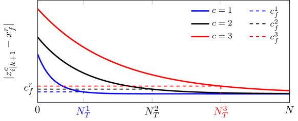
Refer to caption
Figure 2: Sensitivity prediction (solid lines) of (11) for three scenarios at tk+1subscript𝑡𝑘1t_{k+1}, and the terminal regions (below dashed lines). Nk+1subscript𝑁𝑘1N_{k+1} will be reduced from N𝑁N to at least NT3superscriptsubscript𝑁𝑇3N_{T}^{3}.

Fig. 2 is a simple illustration of how a new horizon length is determined for three scenarios. The one-step-ahead prediction of the solution to (11) from a sensitivity update is in solid lines and the terminal regions for each scenario are below the dashed lines. Each scenario reaches its respective terminal region at stage NTcsuperscriptsubscript𝑁𝑇𝑐N_{T}^{c}. To ensure that each scenario reaches its terminal region at tk+1subscript𝑡𝑘1t_{k+1}, the new prediction horizon must be at least equal to the largest NTcsuperscriptsubscript𝑁𝑇𝑐N_{T}^{c}. Therefore in Fig. 2 Nk+1subscript𝑁𝑘1N_{k+1} must be greater than NT3superscriptsubscript𝑁𝑇3N_{T}^{3}.

Algorithm 1 presents the horizon update algorithm for multi-stage MPC.

Algorithm 1 Horizon update for multi-stage MPC
1:Define Nmaxsubscript𝑁maxN_{\text{max}}, Nmin>NRsubscript𝑁minsubscript𝑁𝑅N_{\text{min}}>N_{R}
2:Determine 𝕏frsuperscriptsubscript𝕏𝑓𝑟\mathbb{X}_{f}^{r}, Prsubscript𝑃𝑟P_{r} for all dr𝔻superscript𝑑𝑟𝔻d^{r}\in\mathbb{D}
3:Initialize: k0𝑘0k\leftarrow 0, N0Nmaxsubscript𝑁0subscript𝑁maxN_{0}\leftarrow N_{\text{max}}
4:w(xk)superscript𝑤subscript𝑥𝑘absentw^{\star}(x_{k})\leftarrow Solve (11) with Nksubscript𝑁𝑘N_{k} and initial state xksubscript𝑥𝑘x_{k}
5:𝒳k+1{xk+1r|xk+1r=f(xk,uk,dr)dr𝔻}subscript𝒳𝑘1conditional-setsuperscriptsubscript𝑥𝑘1𝑟superscriptsubscript𝑥𝑘1𝑟𝑓subscript𝑥𝑘subscript𝑢𝑘superscript𝑑𝑟for-allsuperscript𝑑𝑟𝔻\mathcal{X}_{k+1}\leftarrow\{x_{k+1}^{r}\>|\>x_{k+1}^{r}=f(x_{k},u_{k},d^{r})\>\forall d^{r}\in\mathbb{D}\}
6:xkwsubscriptsubscript𝑥𝑘superscript𝑤absent\nabla_{x_{k}}w^{\star}\leftarrow Evaluate (14) to obtain NLP sensitivities at xksubscript𝑥𝑘x_{k}
7:𝒲k+1{getw(xk+1r)using (15)xk+1r𝒳k+1}superscriptsubscript𝒲𝑘1getsuperscript𝑤superscriptsubscript𝑥𝑘1𝑟using (15)for-allsuperscriptsubscript𝑥𝑘1𝑟subscript𝒳𝑘1\mathcal{W}_{k+1}^{\star}\leftarrow\{\text{get}\>w^{\star}(x_{k+1}^{r})\>\text{using \eqref{eq:nlpsenslinearapprox}}\>\forall x_{k+1}^{r}\in\mathcal{X}_{k+1}\}
8:for all w(xk+1r)Wk+1superscript𝑤superscriptsubscript𝑥𝑘1𝑟superscriptsubscript𝑊𝑘1w^{\star}(x_{k+1}^{r})\in W_{k+1}^{\star} do
9:     if zNk|k+1c𝕏frcsubscriptsuperscript𝑧𝑐conditionalsubscript𝑁𝑘𝑘1superscriptsubscript𝕏𝑓𝑟for-all𝑐z^{c}_{N_{k}|k+1}\in\mathbb{X}_{f}^{r}\>\forall c\in\mathbb{C} then
10:         NTcsuperscriptsubscript𝑁𝑇𝑐absentN_{T}^{c}\leftarrow step at which 𝕏frsuperscriptsubscript𝕏𝑓𝑟\mathbb{X}_{f}^{r} is reached
11:         NT(xk+1r)maxcNTcsubscript𝑁𝑇superscriptsubscript𝑥𝑘1𝑟subscriptmax𝑐superscriptsubscript𝑁𝑇𝑐N_{T}(x_{k+1}^{r})\leftarrow\operatorname*{max}_{c\in\mathbb{C}}N_{T}^{c}
12:     else
13:         NT(xk+1r)Nmaxsubscript𝑁𝑇superscriptsubscript𝑥𝑘1𝑟subscript𝑁maxN_{T}(x_{k+1}^{r})\leftarrow N_{\text{max}}
14:     end if
15:end for
16:NTmaxxk+1r𝒳k+1NT(xk+1r)subscript𝑁𝑇subscriptmaxsuperscriptsubscript𝑥𝑘1𝑟subscript𝒳𝑘1subscript𝑁𝑇superscriptsubscript𝑥𝑘1𝑟N_{T}\leftarrow\operatorname*{max}_{x_{k+1}^{r}\in\mathcal{X}_{k+1}}N_{T}(x_{k+1}^{r})
17:Nk+1min(Nmax,NT+Nmin)subscript𝑁𝑘1minsubscript𝑁maxsubscript𝑁𝑇subscript𝑁minN_{k+1}\leftarrow\operatorname*{min}(N_{\text{max}},N_{T}+N_{\text{min}})
18:kk+1𝑘𝑘1k\leftarrow k+1
19:Go to Step 4

The flowchart in Fig. 3 summarizes Algorithm 1 which is a mapping of the current state and prediction horizon to the subsequent prediction horizon. The mapping is defined as a function in 6 as follows:

Refer to caption
Figure 3: Horizon update algorithm for multi-stage MPC that gives admissible prediction horizons for subsequent MPC iterations.
Definition 6.

(Horizon update function) Let 𝒩𝒩\mathcal{N} be the universal set of admissible horizon lengths such that 𝒩={N|NminNNmax,N+}𝒩conditional-set𝑁formulae-sequencesubscript𝑁min𝑁subscript𝑁max𝑁subscript\mathcal{N}=\{N\,|\,N_{\text{min}}\leq N\leq N_{\text{max}},\,N\in\mathbb{Z}_{+}\}. Further, there exists a subset of horizon lengths 𝒩k𝒩subscript𝒩𝑘𝒩\mathcal{N}_{k}\subset\mathcal{N} that define the feasible problems (11) at time tksubscript𝑡𝑘t_{k}. We define a function H:nx×𝒩×nx𝒩:𝐻maps-tosuperscriptsubscript𝑛𝑥𝒩superscriptsubscript𝑛𝑥𝒩H\colon\mathbb{R}^{n_{x}}\times\mathcal{N}\times\mathbb{R}^{n_{x}}\mapsto\mathcal{N} that determines the horizon lengths for the adaptive horizon multi-stage algorithm such that Nk+1=H(xk,Nk,zk+1|kc)𝒩k+1subscript𝑁𝑘1𝐻subscript𝑥𝑘subscript𝑁𝑘subscriptsuperscript𝑧𝑐𝑘conditional1𝑘subscript𝒩𝑘1N_{k+1}=H(x_{k},N_{k},z^{c}_{k+1|k})\in\mathcal{N}_{k+1}.

5 Stability properties of the adaptive horizon multi-stage MPC

Applying the optimal control input computed by the MPC controller to system (1) results in a closed-loop uncertain system whose dynamics are denoted by xk+1=F(xk,dk)subscript𝑥𝑘1𝐹subscript𝑥𝑘subscript𝑑𝑘x_{k+1}=F(x_{k},d_{k}). We will perform a stability analysis for this closed-loop uncertain system. Input-to-state practical stability (ISpS) is the suitable framework to analyze the stability properties of such a system. We start with recollecting some definitions in ISpS stability analysis of discrete-time nonlinear systems:

Definition 7.

(Comparison functions [20]) A function α:++:𝛼maps-tosubscriptsubscript\alpha\colon\mathbb{R}_{+}\mapsto\mathbb{R}_{+} is said to be of class 𝒦𝒦\mathcal{K} if α(0)=0𝛼00\alpha(0)=0, α(n)>0𝛼𝑛0\alpha(n)>0 for all n>0𝑛0n>0 and is strictly increasing. It becomes of class 𝒦subscript𝒦\mathcal{K}_{\infty} if in addition, α𝛼\alpha is unbounded. A function β:+×++:𝛽maps-tosubscriptsubscriptsubscript\beta\colon\mathbb{R}_{+}\times\mathbb{Z}_{+}\mapsto\mathbb{R}_{+} is of class 𝒦𝒦\mathcal{KL} if β(,k)𝛽𝑘\beta(\cdot,k) is of class 𝒦𝒦\mathcal{K} for each fixed k0𝑘0k\geq 0, and β(n,)𝛽𝑛\beta(n,\cdot) is decreasing for each fixed n0𝑛0n\geq 0 and β(n,k)0𝛽𝑛𝑘0\beta(n,k)\rightarrow 0 as k𝑘k\rightarrow\infty.

Definition 8.

(Regional input-to-state practical stability (ISpS), [21]) An autonomous system x+=F(x,d)superscript𝑥𝐹𝑥𝑑x^{+}=F(x,d) is ISpS in ΓnΓsuperscript𝑛\Gamma\subseteq\mathbb{R}^{n} and 0Γ0Γ0\in\Gamma if there exists a 𝒦𝒦\mathcal{KL} function β𝛽\beta, a 𝒦𝒦\mathcal{K} function γ𝛾\gamma, and a constant c0𝑐0c\geq 0 such that for all k0𝑘0k\geq 0

|xk|β(|x0|,k)+γ(𝐝[0,k1]𝐝0)+c,x0Γformulae-sequencesubscript𝑥𝑘𝛽subscript𝑥0𝑘𝛾normsubscript𝐝0𝑘1superscript𝐝0𝑐for-allsubscript𝑥0Γ|x_{k}|\leq\beta(|x_{0}|,k)+\gamma(\|\mathbf{d}_{[0,k-1]}-\mathbf{d}^{0}\|)+c,\quad\forall\,x_{0}\in\Gamma (16)

where 𝐝[0,k1]:=[d0,d1,,dk1]assignsubscript𝐝0𝑘1matrixsubscript𝑑0subscript𝑑1subscript𝑑𝑘1\mathbf{d}_{[0,k-1]}:=\begin{bmatrix}d_{0},&d_{1},&\dots,&d_{k-1}\end{bmatrix} is the sequence of true parameter realizations and 𝐝0superscript𝐝0\mathbf{d}^{0} is a sequence of nominal parameters of the same length.

Definition 9.

(ISpS Lyapunov function in ΓΓ\Gamma, [22]) Suppose ΓΓ\Gamma is an RPI set and there exists a compact set ΘΓΘΓ\Theta\subseteq\Gamma with the origin as an interior point. A function V:n+:𝑉maps-tosuperscript𝑛subscriptV\colon\mathbb{R}^{n}\mapsto\mathbb{R}_{+} is an ISpS Lyapunov function in ΓΓ\Gamma for the system x+=F(x,d)superscript𝑥𝐹𝑥𝑑x^{+}=F(x,d), if there exist 𝒦subscript𝒦\mathcal{K}_{\infty} functions α1subscript𝛼1\alpha_{1}, α2subscript𝛼2\alpha_{2}, α3subscript𝛼3\alpha_{3}, 𝒦𝒦\mathcal{K} function σ𝜎\sigma, and constants c1,c20subscript𝑐1subscript𝑐20c_{1},c_{2}\geq 0 such that:

V(x)𝑉𝑥\displaystyle V(x) α1(|x|),xΓformulae-sequenceabsentsubscript𝛼1𝑥for-all𝑥Γ\displaystyle\geq\alpha_{1}(|x|),\quad\forall\,x\in\Gamma (17a)
V(x)𝑉𝑥\displaystyle V(x) α2(|x|)+c1,xΘformulae-sequenceabsentsubscript𝛼2𝑥subscript𝑐1for-all𝑥Θ\displaystyle\leq\alpha_{2}(|x|)+c_{1},\quad\forall\,x\in\Theta (17b)
V(x+)V(x)α3(|x|)+σ(|dd0|)+c2,xΓ,d,d0Ω.formulae-sequence𝑉superscript𝑥𝑉𝑥subscript𝛼3𝑥𝜎𝑑superscript𝑑0subscript𝑐2formulae-sequencefor-all𝑥Γfor-all𝑑superscript𝑑0Ω\displaystyle\begin{split}V(x^{+})-V(x)&\leq-\alpha_{3}(|x|)+\sigma(|d-d^{0}|)+c_{2},\\ &\quad\forall\,x\in\Gamma,\forall\,d,d^{0}\in\Omega.\end{split} (17c)

where ΩΩ\Omega is the uncertain parameter (disturbance) set.

A standard MPC equivalent with an adaptive horizon can be obtained from (11) by setting dic=di0subscriptsuperscript𝑑𝑐𝑖subscriptsuperscript𝑑0𝑖d^{c}_{i}=d^{0}_{i} for all c𝑐c\in\mathbb{C} as follows:

VNkahm(xk,𝐝0)=subscriptsuperscript𝑉ahmsubscript𝑁𝑘subscript𝑥𝑘superscript𝐝0absent\displaystyle V^{\mathrm{ahm}}_{N_{k}}(x_{k},\mathbf{d}^{0})= minzic,νiccωc(ψ(zNkc,dNk10)+i=0Nk1(zic,νic,di0))subscriptminsuperscriptsubscript𝑧𝑖𝑐superscriptsubscript𝜈𝑖𝑐subscript𝑐subscript𝜔𝑐𝜓superscriptsubscript𝑧subscript𝑁𝑘𝑐superscriptsubscript𝑑subscript𝑁𝑘10superscriptsubscript𝑖0subscript𝑁𝑘1superscriptsubscript𝑧𝑖𝑐superscriptsubscript𝜈𝑖𝑐superscriptsubscript𝑑𝑖0\displaystyle\operatorname*{min}_{z_{i}^{c},\nu_{i}^{c}}\>\sum_{c\in\mathbb{C}}\omega_{c}\Big{(}\psi(z_{N_{k}}^{c},d_{N_{k}-1}^{0})+\sum_{i=0}^{N_{k}-1}\ell(z_{i}^{c},\nu_{i}^{c},d_{i}^{0})\Big{)} (18a)
s.t. zi+1c=f(zic,νic,di0),i=0,,Nk1formulae-sequencesuperscriptsubscript𝑧𝑖1𝑐𝑓superscriptsubscript𝑧𝑖𝑐superscriptsubscript𝜈𝑖𝑐superscriptsubscript𝑑𝑖0𝑖0subscript𝑁𝑘1\displaystyle z_{i+1}^{c}=f(z_{i}^{c},\nu_{i}^{c},d_{i}^{0}),\quad i=0,\dots,N_{k}-1 (18b)
z0c=xk,superscriptsubscript𝑧0𝑐subscript𝑥𝑘\displaystyle z_{0}^{c}=x_{k}, (18c)
νic=νic,{(c,c)|zic=zic}superscriptsubscript𝜈𝑖𝑐superscriptsubscript𝜈𝑖superscript𝑐conditional-set𝑐superscript𝑐superscriptsubscript𝑧𝑖𝑐superscriptsubscript𝑧𝑖superscript𝑐\displaystyle\nu_{i}^{c}=\nu_{i}^{c^{\prime}},\quad\{(c,c^{\prime})\;|\;z_{i}^{c}=z_{i}^{c^{\prime}}\} (18d)
di10=di0,i=NR,,Nk1formulae-sequencesuperscriptsubscript𝑑𝑖10superscriptsubscript𝑑𝑖0𝑖subscript𝑁𝑅subscript𝑁𝑘1\displaystyle d_{i-1}^{0}=d_{i}^{0},\quad i=N_{R},\;\dots,\;N_{k}-1 (18e)
zic𝕏,νic𝕌,di0𝔻,formulae-sequencesuperscriptsubscript𝑧𝑖𝑐𝕏formulae-sequencesuperscriptsubscript𝜈𝑖𝑐𝕌superscriptsubscript𝑑𝑖0𝔻\displaystyle z_{i}^{c}\in\mathbb{X},\>\nu_{i}^{c}\in\mathbb{U},\>d_{i}^{0}\in\mathbb{D}, (18f)
zNkc𝕏fc,superscriptsubscript𝑧subscript𝑁𝑘𝑐superscriptsubscript𝕏𝑓𝑐\displaystyle z_{N_{k}}^{c}\in\mathbb{X}_{f}^{c}, (18g)
c,c,for-all𝑐superscript𝑐\displaystyle\forall\,c,c^{\prime}\in\mathbb{C},\

where (18) effectively consists of c𝑐c identical copies of the standard MPC with an adaptive horizon.

It follows from 3 that the difference between the primal solutions (zi,νi)subscript𝑧𝑖subscript𝜈𝑖(z_{i},\allowbreak\nu_{i}) of (11) and (18) is |w(𝐝c)w(𝐝0)|Ls|Δ𝐝|superscript𝑤superscript𝐝𝑐superscript𝑤superscript𝐝0subscript𝐿𝑠Δ𝐝|w^{\star}(\mathbf{d}^{c})-w^{\star}(\mathbf{d}^{0})|\leq L_{s}|\Delta\mathbf{d}|, where w=[z,ν]superscript𝑤superscriptsuperscriptsuperscript𝑧topsuperscriptsuperscript𝜈toptopw^{\star}=[{z^{\star}}^{\top},{\nu^{\star}}^{\top}]^{\top}, Ls>0subscript𝐿𝑠0L_{s}>0 is the Lipschitz constant, and |Δ𝐝|Δ𝐝|\Delta\mathbf{d}| is defined as:

|Δ𝐝|:=maxdr,dr𝔻|drdr|assignΔ𝐝subscriptmaxsuperscript𝑑𝑟superscript𝑑superscript𝑟𝔻superscript𝑑𝑟superscript𝑑superscript𝑟|\Delta\mathbf{d}|:=\operatorname*{max}_{d^{r},d^{r^{\prime}}\in\mathbb{D}}|d^{r}-d^{r^{\prime}}| (19)

that is the maximum difference in the disturbance vector between any two parameter realizations. Since the evolution of (1) in closed-loop depends on the true disturbance dksubscript𝑑𝑘d_{k}, then xk+1=f(xk,κ(xk),dk)subscript𝑥𝑘1𝑓subscript𝑥𝑘𝜅subscript𝑥𝑘subscript𝑑𝑘x_{k+1}=f(x_{k},\allowbreak\kappa(x_{k}),\allowbreak d_{k}), and xk+1f(xk,κ(xk),dk0)+𝒪(|Δ𝐝|)subscript𝑥𝑘1𝑓subscript𝑥𝑘𝜅subscript𝑥𝑘superscriptsubscript𝑑𝑘0𝒪Δ𝐝x_{k+1}\leq f(x_{k},\allowbreak\kappa(x_{k}),\allowbreak d_{k}^{0})+\mathcal{O}(|\Delta\mathbf{d}|). This result facilitates the recursive feasibility and ISpS stability analysis for the adaptive horizon multi-stage MPC that follows. But first, let us define the following basic assumptions:

Assumption 4.

(Basic assumptions for adaptive horizon multi-stage MPC) The adaptive horizon multi-stage MPC has the following properties:

  1. 1.

    Lipschitz continuity: The functions f𝑓f, \ell, and ψ𝜓\psi are Lipschitz continuous with respect to x𝑥x, u𝑢u and d𝑑d in the compact set 𝕏×𝕌×convhull(𝔻)𝕏𝕌convhull𝔻\mathbb{X}\times\mathbb{U}\times\text{convhull}(\mathbb{D}).

  2. 2.

    Constraint set: The constraint sets 𝕏𝕏\mathbb{X} and 𝕌𝕌\mathbb{U} are compact, and contain the origin in their interiors.

  3. 3.

    The solution to (11) satisfies LICQ and SSOSC such that 3 applies.

With these properties in 4, the Lipschitz continuity holds w.r.t. xksubscript𝑥𝑘x_{k} and 𝐝csuperscript𝐝𝑐\mathbf{d}^{c} for the optimal solution and the optimal cost VNkahmsuperscriptsubscript𝑉subscript𝑁𝑘𝑎𝑚V_{N_{k}}^{ahm}.222The LICQ condition may be relaxed to the Mangasarian-Fromovitz constraint qualification (MFCQ), the constant rank constraint qualification (CRCQ), and the general strong second-order sufficient condition (GSSOSC). In that case, a similar Lipschitz argument can be made and applied in the following analysis. [23, 24]

Assumption 5.

(Property of the stage cost) Given a common control law κ:𝕏𝕌:𝜅maps-to𝕏𝕌\kappa\colon\mathbb{X}\mapsto\mathbb{U} then for any parameter realization dr𝔻superscript𝑑𝑟𝔻d^{r}\in\mathbb{D}, the stage cost \ell is bounded as follows: αp(|x|)(x,κ(x),dr)αq(|x|)+σq(|drd0|)subscript𝛼𝑝𝑥𝑥𝜅𝑥superscript𝑑𝑟subscript𝛼𝑞𝑥subscript𝜎𝑞superscript𝑑𝑟superscript𝑑0\alpha_{p}(|x|)\leq\ell(x,\allowbreak\kappa(x),\allowbreak d^{r})\leq\alpha_{q}(|x|)+\sigma_{q}(|d^{r}-d^{0}|) where αp(),αq()𝒦subscript𝛼𝑝subscript𝛼𝑞subscript𝒦\alpha_{p}(\cdot),\allowbreak\;\alpha_{q}(\cdot)\in\mathcal{K}_{\infty}, and σq()𝒦subscript𝜎𝑞𝒦\sigma_{q}(\cdot)\in\mathcal{K}.

5 requires that the stage cost is positive, with lower and upper bounds proportional to the state at the nominal disturbance. When the disturbance realization is not nominal, the upper bound increases by a term proportional to the distance of the disturbance realization from the nominal.

Assumption 6.

(Assumptions on terminal conditions of the adaptive horizon multi-stage MPC). Let 4 hold for all parameter realizations dr𝔻superscript𝑑𝑟𝔻d^{r}\in\mathbb{D} then:

  1. 1.

    There exists a common terminal region 𝕏f=r𝕏frsubscript𝕏𝑓subscript𝑟superscriptsubscript𝕏𝑓𝑟\mathbb{X}_{f}=\bigcap\limits_{r\in\mathbb{Q}}\mathbb{X}_{f}^{r}, that is robust control invariant.

  2. 2.

    𝕏f𝕏subscript𝕏𝑓𝕏\mathbb{X}_{f}\subseteq\mathbb{X} is compact and contains the origin in its interior.

  3. 3.

    The terminal cost is bounded as follows: αp,ψ(|x|)ψ(x,dr)αq,ψ(|x|)+σq,ψ(|drd0|)subscript𝛼𝑝𝜓𝑥𝜓𝑥superscript𝑑𝑟subscript𝛼𝑞𝜓𝑥subscript𝜎𝑞𝜓superscript𝑑𝑟superscript𝑑0\alpha_{p,\allowbreak\psi}(|x|)\leq\psi(x,\allowbreak d^{r})\leq\alpha_{q,\allowbreak\psi}(|x|)+\sigma_{q,\allowbreak\psi}(|d^{r}-d^{0}|) where αp,ψ,αq,ψ𝒦subscript𝛼𝑝𝜓subscript𝛼𝑞𝜓subscript𝒦\alpha_{p,\allowbreak\psi},\allowbreak\alpha_{q,\allowbreak\psi}\in\mathcal{K}_{\infty}, and σq,ψ𝒦subscript𝜎𝑞𝜓𝒦\sigma_{q,\psi}\in\mathcal{K}.

  4. 4.

    The terminal cost is a local control Lyapunov function ψ(f(x,κf(x),dr),dr)ψ(x,dr)(x,κf(x),dr)𝜓𝑓𝑥subscript𝜅𝑓𝑥superscript𝑑𝑟superscript𝑑𝑟𝜓𝑥superscript𝑑𝑟𝑥subscript𝜅𝑓𝑥superscript𝑑𝑟\psi(f(x,\allowbreak\kappa_{f}(x),\allowbreak d^{r}),\allowbreak d^{r})-\psi(x,\allowbreak d^{r})\leq-\ell(x,\allowbreak\kappa_{f}(x),\allowbreak d^{r}) for all x𝕏f𝑥subscript𝕏𝑓x\in\mathbb{X}_{f}.

61 is needed because a common terminal region must exist for a possible reduction of the prediction horizon. The selection of a prediction horizon where all scenarios reach their respective terminal regions in Step 11 of Algorithm 1 implies that the common terminal region is reached. This region may be a null set when |Δ𝐝|Δ𝐝|\Delta\mathbf{d}| is sufficiently large. Further, this can be determined beforehand when computing the terminal ingredients.

5.1 Recursive feasibility of the adaptive horizon multi-stage MPC with a fully branched scenario tree

Before stability analysis, recursive feasibility must be guaranteed by ensuring robust constraint satisfaction. Given the assumptions above, we first present the following result for a fully branched scenario tree i.e. NR=Nksubscript𝑁𝑅subscript𝑁𝑘N_{R}=N_{k}:

Theorem 4.

(Recursive feasibility of the adaptive horizon multi-stage MPC). Suppose 4, 5 and 6 hold, then problem (11) from a fully branched scenario tree NR=Nksubscript𝑁𝑅subscript𝑁𝑘N_{R}=N_{k} is recursively feasible.

Proof.

Let 4 and 6 hold and consider the fully branched multi-stage MPC with NR=Nksubscript𝑁𝑅subscript𝑁𝑘N_{R}=N_{k}. Proposition 4 in [25] and Theorem 6 in [26] show that if a robust control invariant terminal region exists then the fully branched multi-stage MPC with a fixed horizon NR=Nksubscript𝑁𝑅subscript𝑁𝑘N_{R}=N_{k} is recursively feasible. Since the adaptive horizon, multi-stage MPC with NR=Nksubscript𝑁𝑅subscript𝑁𝑘N_{R}=N_{k} ensures that the horizon is updated such that the common terminal region is always reached, it is also recursively feasible for any horizon update Nk+1subscript𝑁𝑘1N_{k+1} given by Algorithm 1. ∎

5.2 Recursive feasibility of the adaptive horizon multi-stage MPC with a robust horizon

Recursive feasibility cannot be guaranteed by using the same arguments in 4 when the scenario tree is not fully branched. But the infeasibility of problem (11) when NR<Nksubscript𝑁𝑅subscript𝑁𝑘N_{R}<N_{k} may be avoided by relaxing the state inequalities using soft constraints [27]. However, robust constraint satisfaction is not guaranteed because the state trajectories may cross the feasible set 𝕏𝕏\mathbb{X}. Therefore, before proceeding to the stability analysis the following assumption must be made:

Assumption 7.

Problem (11) is feasible at time tksubscript𝑡𝑘t_{k} when Nk=Nmaxsubscript𝑁𝑘subscript𝑁maxN_{k}=N_{\text{max}}. Furthermore, if problem (11) at time tksubscript𝑡𝑘t_{k} with xksubscript𝑥𝑘x_{k} and Nksubscript𝑁𝑘N_{k} is feasible, then so is problem (11) solved at time tk+1subscript𝑡𝑘1t_{k+1} with xk+1subscript𝑥𝑘1x_{k+1} and Nk+1=H(xk,Nk,xk+1)𝒩k+1subscript𝑁𝑘1𝐻subscript𝑥𝑘subscript𝑁𝑘subscript𝑥𝑘1subscript𝒩𝑘1N_{k+1}=H(x_{k},N_{k},x_{k+1})\in\mathcal{N}_{k+1} for all xk,xk+1𝕏subscript𝑥𝑘subscript𝑥𝑘1𝕏x_{k},x_{k+1}\in\mathbb{X}, Nk𝒩k+1subscript𝑁𝑘subscript𝒩𝑘1N_{k}\in\mathcal{N}_{k+1}.

Note that 7 can always be satisfied by choosing NR=Nksubscript𝑁𝑅subscript𝑁𝑘N_{R}=N_{k}. (cf. Theorem 4). The increase in the problem size with a long robust horizon required to satisfy 7 also motivates the need for shortening the horizon length using our proposed Algorithm 1. 7 ensures that H𝐻H (see 6) produces feasible horizon lengths for any robust horizon NRNksubscript𝑁𝑅subscript𝑁𝑘N_{R}\leq N_{k}, essentially implying recursive feasibility. This allows us to present results on the ISpS property of the adaptive horizon multi-stage MPC.

5.3 ISpS for adaptive horizon multi-stage MPC

First, the relationships between the linear and nonlinear systems are needed because the nonlinear system (1) is controlled by a stabilizing linear controller inside the common terminal region 𝕏fsubscript𝕏𝑓\mathbb{X}_{f}. Consider the nominal problem (18) inside the terminal region evaluated using a stabilizing terminal control law κf0superscriptsubscript𝜅𝑓0\kappa_{f}^{0}:

VNlqr(xk,𝐝0):=cωc(ψ(zN0,dN10)+i=0N1(zi0,κf0(zi0),di0))assignsuperscriptsubscript𝑉𝑁lqrsubscript𝑥𝑘superscript𝐝0subscript𝑐subscript𝜔𝑐𝜓subscriptsuperscript𝑧0𝑁superscriptsubscript𝑑𝑁10subscriptsuperscript𝑁1𝑖0subscriptsuperscript𝑧0𝑖superscriptsubscript𝜅𝑓0subscriptsuperscript𝑧0𝑖subscriptsuperscript𝑑0𝑖V_{N}^{\mathrm{lqr}}(x_{k},\mathbf{d}^{0}):=\sum_{c\in\mathbb{C}}\omega_{c}\Big{(}\psi(z^{0}_{N},d_{N-1}^{0})+\sum^{N-1}_{i=0}\ell(z^{0}_{i},\kappa_{f}^{0}(z^{0}_{i}),d^{0}_{i})\Big{)}\\ (20)

where zi+10=A0zi0+B0νi0+ψ(zi0,d0),i=0,,N1formulae-sequencesubscriptsuperscript𝑧0𝑖1subscript𝐴0subscriptsuperscript𝑧0𝑖subscript𝐵0subscriptsuperscript𝜈0𝑖𝜓subscriptsuperscript𝑧0𝑖superscript𝑑0for-all𝑖0𝑁1z^{0}_{i+1}=A_{0}z^{0}_{i}+B_{0}\nu^{0}_{i}+\psi(z^{0}_{i},d^{0}),\;\forall i=0,\dots,N-1, and VNlqr(xk,𝐝0)superscriptsubscript𝑉𝑁𝑙𝑞𝑟subscript𝑥𝑘superscript𝐝0V_{N}^{lqr}(x_{k},\mathbf{d}^{0}) is the nominal LQR cost. The relationships between the optimal costs of the nominal equivalents of the LQR and adaptive horizon multi-stage MPC in the terminal region are given in 5.

Lemma 5.

(Effect of linearization on costs inside the terminal region) There exists αn𝒦subscript𝛼𝑛subscript𝒦\alpha_{n}\in\mathcal{K}_{\infty} such that |VNlqr(x,𝐝0)ψ(x,d0)|αn(|x|)subscriptsuperscript𝑉lqr𝑁𝑥superscript𝐝0𝜓𝑥superscript𝑑0subscript𝛼𝑛𝑥|V^{\mathrm{lqr}}_{N}(x,\mathbf{d}^{0})-\psi(x,d^{0})|\leq\alpha_{n}(|x|) and αv𝒦subscript𝛼𝑣subscript𝒦\alpha_{v}\in\mathcal{K}_{\infty} such that |ψ(x,d0)VNahm(x,𝐝0)|αv(|x|)𝜓𝑥superscript𝑑0superscriptsubscript𝑉𝑁ahm𝑥superscript𝐝0subscript𝛼𝑣𝑥|\psi(x,d^{0})-V_{N}^{\mathrm{ahm}}(x,\mathbf{d}^{0})|\leq\alpha_{v}(|x|) for all x𝕏f𝑥subscript𝕏𝑓x\in\mathbb{X}_{f} and for all N𝒩𝑁𝒩N\in\mathcal{N}.

Proof.

Because this is a nominal problem, the result holds because of Lemmas 18 and 19 in [9]. ∎

Assumption 8.

The solution to (18) with a prediction horizon NkNminsubscript𝑁𝑘subscript𝑁minN_{k}\geq N_{\text{min}} satisfies:

αn(|zNk|k0|)αp(|xk|)subscript𝛼𝑛subscriptsuperscript𝑧0conditionalsubscript𝑁𝑘𝑘subscript𝛼𝑝subscript𝑥𝑘\displaystyle\alpha_{n}(|z^{0}_{N_{k}|k}|)-\alpha_{p}(|x_{k}|) α3(|xk|) if Nk+1Nkabsentsubscript𝛼3subscript𝑥𝑘 if subscript𝑁𝑘1subscript𝑁𝑘\displaystyle\leq-\alpha_{3}(|x_{k}|)\text{ if }N_{k+1}\geq N_{k} (21a)
αv(|zNk+1+1|k0|)αp(|xk|)subscript𝛼𝑣subscriptsuperscript𝑧0subscript𝑁𝑘1conditional1𝑘subscript𝛼𝑝subscript𝑥𝑘\displaystyle\alpha_{v}(|z^{0}_{N_{k+1}+1|k}|)-\alpha_{p}(|x_{k}|) α3(|xk|) if Nk+1<Nkabsentsubscript𝛼3subscript𝑥𝑘 if subscript𝑁𝑘1subscript𝑁𝑘\displaystyle\leq-\alpha_{3}(|x_{k}|)\text{ if }N_{k+1}<N_{k} (21b)

for some α3𝒦subscript𝛼3subscript𝒦\alpha_{3}\in\mathcal{K}_{\infty}, where Nk+1=H(xk,Nk,zk+1|k0)𝒩k+1subscript𝑁𝑘1𝐻subscript𝑥𝑘subscript𝑁𝑘subscriptsuperscript𝑧0𝑘conditional1𝑘subscript𝒩𝑘1N_{k+1}=H(x_{k},N_{k},z^{0}_{k+1|k})\in\mathcal{N}_{k+1}, αpsubscript𝛼𝑝\alpha_{p} satisfy 5, and αnsubscript𝛼𝑛\alpha_{n}, αvsubscript𝛼𝑣\alpha_{v} satisfy 5.

This assumption implies that the approximation error from using the stabilizing linear control law inside the terminal region must be negligible. 8 can be satisfied by finding a suitably large Nminsubscript𝑁minN_{\text{min}} that is determined through simulations as explained in [9].

Theorem 6.

(ISpS stability of adaptive horizon multi-stage MPC) Suppose 5 and 6 hold for (11), the optimal value function Vahmsuperscript𝑉𝑎𝑚V^{ahm} is an ISpS Lyapunov function and the resulting closed-loop system is ISpS stable.

Proof.

To show the ISpS property of the adaptive horizon multi-stage MPC, a Lyapunov function must exist that satisfies the three conditions in (17).

Lower bound: Suppose 5 holds then there exists a lower bound (17a) on the optimal value function.

VNahm(xk,𝐝c)(xk,κN(xk),d00)αp(|xk|)xk𝕏formulae-sequencesuperscriptsubscript𝑉𝑁ahmsubscript𝑥𝑘superscript𝐝𝑐subscript𝑥𝑘subscript𝜅𝑁subscript𝑥𝑘superscriptsubscript𝑑00subscript𝛼𝑝subscript𝑥𝑘for-allsubscript𝑥𝑘𝕏V_{N}^{\mathrm{ahm}}(x_{k},\mathbf{d}^{c})\geq\ell(x_{k},\kappa_{N}(x_{k}),d_{0}^{0})\geq\alpha_{p}(|x_{k}|)\quad\forall x_{k}\in\mathbb{X} (22)

Upper bound: The existence of an upper bound (17b) is shown by using 41, the boundedness property of the optimal cost of standard MPC recursively forward [1], and 63 as follows:

VNahm(xk,𝐝c)superscriptsubscript𝑉𝑁ahmsubscript𝑥𝑘superscript𝐝𝑐\displaystyle V_{N}^{\mathrm{ahm}}(x_{k},\mathbf{d}^{c}) VNahm(xk,𝐝0)+Lv|Δ𝐝|absentsuperscriptsubscript𝑉𝑁ahmsubscript𝑥𝑘superscript𝐝0subscript𝐿𝑣Δ𝐝\displaystyle\leq V_{N}^{\mathrm{ahm}}(x_{k},\mathbf{d}^{0})+L_{v}|\Delta\mathbf{d}| (23a)
ψ(xk,d0)+Lv|Δ𝐝|absent𝜓subscript𝑥𝑘superscript𝑑0subscript𝐿𝑣Δ𝐝\displaystyle\leq\psi(x_{k},d^{0})+L_{v}|\Delta\mathbf{d}| (23b)
αq,ψ(|xk|)+c1absentsubscript𝛼𝑞𝜓subscript𝑥𝑘subscript𝑐1\displaystyle\leq\alpha_{q,\psi}(|x_{k}|)+c_{1} (23c)

for all xk𝕏fsubscript𝑥𝑘subscript𝕏𝑓x_{k}\in\mathbb{X}_{f}, where c1=Lv|Δ𝐝|subscript𝑐1subscript𝐿𝑣Δ𝐝c_{1}=L_{v}|\Delta\mathbf{d}| is a constant. It also applies to all xk𝕏subscript𝑥𝑘𝕏x_{k}\in\mathbb{X} by induction because 𝕏f𝕏subscript𝕏𝑓𝕏\mathbb{X}_{f}\subseteq\mathbb{X}, and VNahm(xk,𝐝0)superscriptsubscript𝑉𝑁ahmsubscript𝑥𝑘superscript𝐝0V_{N}^{\mathrm{ahm}}(x_{k},\mathbf{d}^{0}) is continuous at the origin.

Note that the adaptive horizon multi-stage MPC control law may be discontinuous because it optimizes with different prediction horizons provided by Algorithm 1 at each time step. However, our analysis considers the properties of the optimal cost function VNkahmsuperscriptsubscript𝑉subscript𝑁𝑘𝑎𝑚V_{N_{k}}^{ahm} which may still be continuous even with a discontinuous control law, given that the input constraint set is continuous. [1]

Function descent: The descent property (17c), which is the main part of stability analysis, is shown for two possible cases of horizon update:

1. A decreasing prediction horizon NRNk+1<Nksubscript𝑁𝑅subscript𝑁𝑘1subscript𝑁𝑘N_{R}\leq N_{k+1}<N_{k}: An approximate solution for (18) at time tk+1subscript𝑡𝑘1t_{k+1} is found by shifting the optimal solution at time tksubscript𝑡𝑘t_{k} as follows:

ν^i|k+10=νi+1|k0,i=0,,Nk+11,formulae-sequencesuperscriptsubscript^𝜈conditional𝑖𝑘10superscriptsubscript𝜈𝑖conditional1𝑘0𝑖0subscript𝑁𝑘11\hat{\nu}_{i|k+1}^{0}=\nu_{i+1|k}^{0},\quad\;i=0,\dots,N_{k+1}-1, (24)

and the corresponding initialization for state variables:

z^0|k+10=z1|k0,superscriptsubscript^𝑧conditional0𝑘10superscriptsubscript𝑧conditional1𝑘0\displaystyle\hat{z}_{0|k+1}^{0}=z_{1|k}^{0}, (25a)
z^i+1|k+10=f(z^i|k0,ν^i|k0,di0)superscriptsubscript^𝑧𝑖conditional1𝑘10𝑓superscriptsubscript^𝑧conditional𝑖𝑘0superscriptsubscript^𝜈conditional𝑖𝑘0superscriptsubscript𝑑𝑖0\displaystyle\hat{z}_{i+1|k+1}^{0}=f(\hat{z}_{i|k}^{0},\hat{\nu}_{i|k}^{0},d_{i}^{0}) (25b)

leads to a suboptimal cost such that the descent inequality becomes:

VNk+1ahm(f(xk,κ(xk),d00),𝐝0)VNkahm(xk,𝐝0)cωc(ψ(z^Nk+1|k+10,dNk+110)+i=0Nk+11(z^i|k+10,ν^i|k+10,di0))cωc(ψ(νNk|k0,dNk10)i=0Nk1(zi|k0,νi|k0,di0))superscriptsubscript𝑉subscript𝑁𝑘1ahm𝑓subscript𝑥𝑘𝜅subscript𝑥𝑘superscriptsubscript𝑑00superscript𝐝0superscriptsubscript𝑉subscript𝑁𝑘ahmsubscript𝑥𝑘superscript𝐝0subscript𝑐subscript𝜔𝑐𝜓superscriptsubscript^𝑧conditionalsubscript𝑁𝑘1𝑘10superscriptsubscript𝑑subscript𝑁𝑘110superscriptsubscript𝑖0subscript𝑁𝑘11superscriptsubscript^𝑧conditional𝑖𝑘10superscriptsubscript^𝜈conditional𝑖𝑘10superscriptsubscript𝑑𝑖0subscript𝑐subscript𝜔𝑐𝜓superscriptsubscript𝜈conditionalsubscript𝑁𝑘𝑘0superscriptsubscript𝑑subscript𝑁𝑘10superscriptsubscript𝑖0subscript𝑁𝑘1superscriptsubscript𝑧conditional𝑖𝑘0superscriptsubscript𝜈conditional𝑖𝑘0superscriptsubscript𝑑𝑖0\displaystyle\begin{split}&V_{N_{k+1}}^{\mathrm{ahm}}(f(x_{k},\kappa(x_{k}),d_{0}^{0}),\mathbf{d}^{0})-V_{N_{k}}^{\mathrm{ahm}}(x_{k},\mathbf{d}^{0})\\ &\leq\sum_{c\in\mathbb{C}}\omega_{c}\Big{(}\psi(\hat{z}_{N_{k+1}|k+1}^{0},d_{N_{k+1}-1}^{0})+\sum_{i=0}^{N_{k+1}-1}\ell(\hat{z}_{i|k+1}^{0},\hat{\nu}_{i|k+1}^{0},d_{i}^{0})\Big{)}\\ &-\sum_{c\in\mathbb{C}}\omega_{c}\Big{(}\psi(\nu_{N_{k}|k}^{0},d_{N_{k}-1}^{0})-\sum_{i=0}^{N_{k}-1}\ell(z_{i|k}^{0},\nu_{i|k}^{0},d_{i}^{0})\Big{)}\end{split} (26a)
=(xk,κ(xk),d00)+ψ(z^Nk+1|k+10,dNk+110)+i=0Nk+11((z^i|k+10,ν^i|k+10,di0)(zi+1|k0,νi+1|k0,di0))ψ(zNk|k0,dNk10)i=Nk+1+1Nk1(z^i|k0,ν^i|k0,di0)absentsubscript𝑥𝑘𝜅subscript𝑥𝑘superscriptsubscript𝑑00𝜓superscriptsubscript^𝑧conditionalsubscript𝑁𝑘1𝑘10superscriptsubscript𝑑subscript𝑁𝑘110superscriptsubscript𝑖0subscript𝑁𝑘11superscriptsubscript^𝑧conditional𝑖𝑘10superscriptsubscript^𝜈conditional𝑖𝑘10superscriptsubscript𝑑𝑖0superscriptsubscript𝑧𝑖conditional1𝑘0superscriptsubscript𝜈𝑖conditional1𝑘0superscriptsubscript𝑑𝑖0𝜓superscriptsubscript𝑧conditionalsubscript𝑁𝑘𝑘0superscriptsubscript𝑑subscript𝑁𝑘10superscriptsubscript𝑖subscript𝑁𝑘11subscript𝑁𝑘1superscriptsubscript^𝑧conditional𝑖𝑘0superscriptsubscript^𝜈conditional𝑖𝑘0superscriptsubscript𝑑𝑖0\displaystyle\begin{split}&=-\ell(x_{k},\kappa(x_{k}),d_{0}^{0})+\psi(\hat{z}_{N_{k+1}|k+1}^{0},d_{N_{k+1}-1}^{0})\\ &+\sum_{i=0}^{N_{k+1}-1}\big{(}\ell(\hat{z}_{i|k+1}^{0},\hat{\nu}_{i|k+1}^{0},d_{i}^{0})-\ell(z_{i+1|k}^{0},\nu_{i+1|k}^{0},d_{i}^{0})\big{)}\\ &-\psi(z_{N_{k}|k}^{0},d_{N_{k}-1}^{0})-\sum_{i=N_{k+1}+1}^{N_{k}-1}\ell(\hat{z}_{i|k}^{0},\hat{\nu}_{i|k}^{0},d_{i}^{0})\end{split} (26b)
=(xk,κ(xk),d00)+ψ(z^Nk+1|k+10,dNk+110)ψ(zNk|k0,dNk10)i=Nk+1+1Nk1(z^i|k0,ν^i|k0,di0)absentsubscript𝑥𝑘𝜅subscript𝑥𝑘superscriptsubscript𝑑00𝜓superscriptsubscript^𝑧conditionalsubscript𝑁𝑘1𝑘10superscriptsubscript𝑑subscript𝑁𝑘110𝜓superscriptsubscript𝑧conditionalsubscript𝑁𝑘𝑘0superscriptsubscript𝑑subscript𝑁𝑘10superscriptsubscript𝑖subscript𝑁𝑘11subscript𝑁𝑘1superscriptsubscript^𝑧conditional𝑖𝑘0superscriptsubscript^𝜈conditional𝑖𝑘0superscriptsubscript𝑑𝑖0\displaystyle\begin{split}&=-\ell(x_{k},\kappa(x_{k}),d_{0}^{0})+\psi(\hat{z}_{N_{k+1}|k+1}^{0},d_{N_{k+1}-1}^{0})\\ &-\psi(z_{N_{k}|k}^{0},d_{N_{k}-1}^{0})-\sum_{i=N_{k+1}+1}^{N_{k}-1}\ell(\hat{z}_{i|k}^{0},\hat{\nu}_{i|k}^{0},d_{i}^{0})\end{split} (26c)
=(xk,κ(xk),d00)+ψ(z^Nk+1|k+10,dNk+110)VNkNk+11ahm(zNk+1+1|k0,𝐝0)absentsubscript𝑥𝑘𝜅subscript𝑥𝑘superscriptsubscript𝑑00𝜓superscriptsubscript^𝑧conditionalsubscript𝑁𝑘1𝑘10superscriptsubscript𝑑subscript𝑁𝑘110superscriptsubscript𝑉subscript𝑁𝑘subscript𝑁𝑘11ahmsuperscriptsubscript𝑧subscript𝑁𝑘1conditional1𝑘0superscript𝐝0\displaystyle\begin{split}&=-\ell(x_{k},\kappa(x_{k}),d_{0}^{0})\\ &+\psi(\hat{z}_{N_{k+1}|k+1}^{0},d_{N_{k+1}-1}^{0})-V_{N_{k}-N_{k+1}-1}^{\mathrm{ahm}}(z_{N_{k+1}+1|k}^{0},\mathbf{d}^{0})\end{split} (26d)
In the presence of true uncertainty, the successor state is xk+1=f(xk,κ(xk),dk)subscript𝑥𝑘1𝑓subscript𝑥𝑘𝜅subscript𝑥𝑘subscript𝑑𝑘x_{k+1}=f(x_{k},\kappa(x_{k}),d_{k}) where dksubscript𝑑𝑘d_{k} is the true parameter realization, such that:
VNk+1ahm(xk+1,𝐝0)VNkahm(xk,𝐝0)(xk,κ(xk),d00)+ψ(z^Nk+1|k+10,dNk+110)VNkNk+11ahm(zNk+1+1|k0,𝐝0)+Lk|dkdi0|superscriptsubscript𝑉subscript𝑁𝑘1ahmsubscript𝑥𝑘1superscript𝐝0superscriptsubscript𝑉subscript𝑁𝑘ahmsubscript𝑥𝑘superscript𝐝0subscript𝑥𝑘𝜅subscript𝑥𝑘superscriptsubscript𝑑00𝜓superscriptsubscript^𝑧conditionalsubscript𝑁𝑘1𝑘10superscriptsubscript𝑑subscript𝑁𝑘110superscriptsubscript𝑉subscript𝑁𝑘subscript𝑁𝑘11ahmsuperscriptsubscript𝑧subscript𝑁𝑘1conditional1𝑘0superscript𝐝0subscript𝐿𝑘subscript𝑑𝑘superscriptsubscript𝑑𝑖0\displaystyle\begin{split}&V_{N_{k+1}}^{\mathrm{ahm}}(x_{k+1},\mathbf{d}^{0})-V_{N_{k}}^{\mathrm{ahm}}(x_{k},\mathbf{d}^{0})\leq-\ell(x_{k},\kappa(x_{k}),d_{0}^{0})\\ &+\psi(\hat{z}_{N_{k+1}|k+1}^{0},d_{N_{k+1}-1}^{0})-V_{N_{k}-N_{k+1}-1}^{\mathrm{ahm}}(z_{N_{k+1}+1|k}^{0},\mathbf{d}^{0})\\ &+L_{k}|d_{k}-d_{i}^{0}|\end{split} (26e)

Then from Eqs. 11 and 18 we have:

VNkahm(xk,𝐝c)superscriptsubscript𝑉subscript𝑁𝑘ahmsubscript𝑥𝑘superscript𝐝𝑐\displaystyle V_{N_{k}}^{\mathrm{ahm}}(x_{k},\mathbf{d}^{c}) =VNkahm(xk,𝐝0)+𝒪(|Δ𝐝|),andabsentsuperscriptsubscript𝑉subscript𝑁𝑘ahmsubscript𝑥𝑘superscript𝐝0𝒪Δ𝐝and\displaystyle=V_{N_{k}}^{\mathrm{ahm}}(x_{k},\mathbf{d}^{0})+\mathcal{O}(|\Delta\mathbf{d}|),\>\text{and} (27a)
VNk+1ahm(xk+1,𝐝c)superscriptsubscript𝑉subscript𝑁𝑘1ahmsubscript𝑥𝑘1superscript𝐝𝑐\displaystyle V_{N_{k+1}}^{\mathrm{ahm}}(x_{k+1},\mathbf{d}^{c}) =VNk+1ahm(xk+1,𝐝0)+𝒪(|Δ𝐝|)absentsuperscriptsubscript𝑉subscript𝑁𝑘1ahmsubscript𝑥𝑘1superscript𝐝0𝒪Δ𝐝\displaystyle=V_{N_{k+1}}^{\mathrm{ahm}}(x_{k+1},\mathbf{d}^{0})+\mathcal{O}(|\Delta\mathbf{d}|) (27b)

that can be combined with (26e) to form:

VNk+1ahm(xk+1,𝐝c)VNkahm(xk,𝐝c)(xk,κ(xk),d00)+ψ(z^Nk+1|k+10,dNk+110)VNkNk+11ahm(zNk+1+1|k0,𝐝0)+Lk|dkdi0|+(VNk+1ahm(xk+1,𝐝c)VNk+1ahm(xk+1,𝐝0))+(VNkahm(xk,𝐝c)VNkahm(xk,𝐝0))superscriptsubscript𝑉subscript𝑁𝑘1ahmsubscript𝑥𝑘1superscript𝐝𝑐superscriptsubscript𝑉subscript𝑁𝑘ahmsubscript𝑥𝑘superscript𝐝𝑐subscript𝑥𝑘𝜅subscript𝑥𝑘superscriptsubscript𝑑00𝜓superscriptsubscript^𝑧conditionalsubscript𝑁𝑘1𝑘10superscriptsubscript𝑑subscript𝑁𝑘110superscriptsubscript𝑉subscript𝑁𝑘subscript𝑁𝑘11ahmsuperscriptsubscript𝑧subscript𝑁𝑘1conditional1𝑘0superscript𝐝0subscript𝐿𝑘subscript𝑑𝑘superscriptsubscript𝑑𝑖0superscriptsubscript𝑉subscript𝑁𝑘1ahmsubscript𝑥𝑘1superscript𝐝𝑐superscriptsubscript𝑉subscript𝑁𝑘1ahmsubscript𝑥𝑘1superscript𝐝0superscriptsubscript𝑉subscript𝑁𝑘ahmsubscript𝑥𝑘superscript𝐝𝑐superscriptsubscript𝑉subscript𝑁𝑘ahmsubscript𝑥𝑘superscript𝐝0\displaystyle\begin{split}&V_{N_{k+1}}^{\mathrm{ahm}}(x_{k+1},\mathbf{d}^{c})-V_{N_{k}}^{\mathrm{ahm}}(x_{k},\mathbf{d}^{c})\leq-\ell(x_{k},\kappa(x_{k}),d_{0}^{0})\\ &+\psi(\hat{z}_{N_{k+1}|k+1}^{0},d_{N_{k+1}-1}^{0})-V_{N_{k}-N_{k+1}-1}^{\mathrm{ahm}}(z_{N_{k+1}+1|k}^{0},\mathbf{d}^{0})\\ &+L_{k}|d_{k}-d_{i}^{0}|+\Big{(}V_{N_{k+1}}^{\mathrm{ahm}}(x_{k+1},\mathbf{d}^{c})-V_{N_{k+1}}^{\mathrm{ahm}}(x_{k+1},\mathbf{d}^{0})\Big{)}\\ &+\Big{(}V_{N_{k}}^{\mathrm{ahm}}(x_{k},\mathbf{d}^{c})-V_{N_{k}}^{\mathrm{ahm}}(x_{k},\mathbf{d}^{0})\Big{)}\end{split} (28a)
(xk,κ(xk),d00)+ψ(z^Nk+1|k+10,dNk+110)VNkNk+11ahm(zNk+1+1|k0,𝐝0)+Lk|dkdi0|+2Lv|Δ𝐝|absentsubscript𝑥𝑘𝜅subscript𝑥𝑘superscriptsubscript𝑑00𝜓superscriptsubscript^𝑧conditionalsubscript𝑁𝑘1𝑘10superscriptsubscript𝑑subscript𝑁𝑘110superscriptsubscript𝑉subscript𝑁𝑘subscript𝑁𝑘11ahmsuperscriptsubscript𝑧subscript𝑁𝑘1conditional1𝑘0superscript𝐝0subscript𝐿𝑘subscript𝑑𝑘superscriptsubscript𝑑𝑖02subscript𝐿𝑣Δ𝐝\displaystyle\begin{split}&\leq-\ell(x_{k},\kappa(x_{k}),d_{0}^{0})+\psi(\hat{z}_{N_{k+1}|k+1}^{0},d_{N_{k+1}-1}^{0})\\ &-V_{N_{k}-N_{k+1}-1}^{\mathrm{ahm}}(z_{N_{k+1}+1|k}^{0},\mathbf{d}^{0})+L_{k}|d_{k}-d_{i}^{0}|+2L_{v}|\Delta\mathbf{d}|\end{split} (28b)
αp(|xk|)+αv(|zNk+1+1|k0|)+Lk|dkdi0|+2Lv|Δ𝐝|absentsubscript𝛼𝑝subscript𝑥𝑘subscript𝛼𝑣superscriptsubscript𝑧subscript𝑁𝑘1conditional1𝑘0subscript𝐿𝑘subscript𝑑𝑘superscriptsubscript𝑑𝑖02subscript𝐿𝑣Δ𝐝\displaystyle\leq-\alpha_{p}(|x_{k}|)+\alpha_{v}(|z_{N_{k+1}+1|k}^{0}|)+L_{k}|d_{k}-d_{i}^{0}|+2L_{v}|\Delta\mathbf{d}| (28c)
α3(|xk|)+σ(|dkdi0|)+c2absentsubscript𝛼3subscript𝑥𝑘𝜎subscript𝑑𝑘superscriptsubscript𝑑𝑖0subscript𝑐2\displaystyle\leq-\alpha_{3}(|x_{k}|)+\sigma(|d_{k}-d_{i}^{0}|)+c_{2} (28d)

where c2=2Lv|Δ𝐝|0subscript𝑐22subscript𝐿𝑣Δ𝐝0c_{2}=2L_{v}|\Delta\mathbf{d}|\geq 0 and (28c) follows from 5 and (28d) follows from (21b).

2. An increasing prediction horizon Nk+1Nksubscript𝑁𝑘1subscript𝑁𝑘N_{k+1}\geq N_{k}: Similar to the first case approximate the solution of (18) at tk+1subscript𝑡𝑘1t_{k+1} by shifting:

ν^i|k+10={νi+1|k0i=0,,Nk2K0zi0i=Nk1,,Nk+11superscriptsubscript^𝜈conditional𝑖𝑘10casessuperscriptsubscript𝜈𝑖conditional1𝑘0for-all𝑖0subscript𝑁𝑘2subscript𝐾0superscriptsubscript𝑧𝑖0for-all𝑖subscript𝑁𝑘1subscript𝑁𝑘11\hat{\nu}_{i|k+1}^{0}=\begin{cases}\nu_{i+1|k}^{0}&\quad\forall\;i=0,\dots,N_{k}-2\\ -K_{0}z_{i}^{0}&\quad\forall\;i=N_{k}-1,\dots,N_{k+1}-1\end{cases}\\ (29)

The initialization of the states is the same as in (25). Then the descent inequality becomes:

VNk+1ahm(f(xk,κ(xk),d00),𝐝0)VNkahm(xk,𝐝0)superscriptsubscript𝑉subscript𝑁𝑘1ahm𝑓subscript𝑥𝑘𝜅subscript𝑥𝑘superscriptsubscript𝑑00superscript𝐝0superscriptsubscript𝑉subscript𝑁𝑘ahmsubscript𝑥𝑘superscript𝐝0\displaystyle V_{N_{k+1}}^{\mathrm{ahm}}(f(x_{k},\kappa(x_{k}),d_{0}^{0}),\mathbf{d}^{0})-V_{N_{k}}^{\mathrm{ahm}}(x_{k},\mathbf{d}^{0}) (30a)
cωc(ψ(z^Nk+1|k+10,dNk+110)+i=0Nk+11(z^i|k+10,ν^i|k+10,dl0))cωc(ψ(zNk|k0,dNk10)i=0Nk1(zi|k0,νi|k0,di0))absentsubscript𝑐subscript𝜔𝑐𝜓superscriptsubscript^𝑧conditionalsubscript𝑁𝑘1𝑘10superscriptsubscript𝑑subscript𝑁𝑘110superscriptsubscript𝑖0subscript𝑁𝑘11superscriptsubscript^𝑧conditional𝑖𝑘10superscriptsubscript^𝜈conditional𝑖𝑘10superscriptsubscript𝑑𝑙0subscript𝑐subscript𝜔𝑐𝜓superscriptsubscript𝑧conditionalsubscript𝑁𝑘𝑘0superscriptsubscript𝑑subscript𝑁𝑘10superscriptsubscript𝑖0subscript𝑁𝑘1superscriptsubscript𝑧conditional𝑖𝑘0superscriptsubscript𝜈conditional𝑖𝑘0superscriptsubscript𝑑𝑖0\displaystyle\begin{split}&\leq\sum_{c\in\mathbb{C}}\omega_{c}\Big{(}\psi(\hat{z}_{N_{k+1}|k+1}^{0},d_{N_{k+1}-1}^{0})+\sum_{i=0}^{N_{k+1}-1}\ell(\hat{z}_{i|k+1}^{0},\hat{\nu}_{i|k+1}^{0},d_{l}^{0})\Big{)}\\ &-\sum_{c\in\mathbb{C}}\omega_{c}\Big{(}\psi(z_{N_{k}|k}^{0},d_{N_{k}-1}^{0})-\sum_{i=0}^{N_{k}-1}\ell(z_{i|k}^{0},\nu_{i|k}^{0},d_{i}^{0})\Big{)}\end{split} (30b)
=(xk,κ(xk),d00)+i=0Nk2((z^i|k+10,ν^i|k+10,di0)(zi+1|k0,νi+1|k0,di0))+ψ(z^Nk+1|k+10,dNk+110)+i=Nk1Nk+11(z^i|k0,ν^i|k0,di0)ψ(zNk|k0,dNk10)absentsubscript𝑥𝑘𝜅subscript𝑥𝑘superscriptsubscript𝑑00superscriptsubscript𝑖0subscript𝑁𝑘2superscriptsubscript^𝑧conditional𝑖𝑘10superscriptsubscript^𝜈conditional𝑖𝑘10superscriptsubscript𝑑𝑖0superscriptsubscript𝑧𝑖conditional1𝑘0superscriptsubscript𝜈𝑖conditional1𝑘0superscriptsubscript𝑑𝑖0𝜓superscriptsubscript^𝑧conditionalsubscript𝑁𝑘1𝑘10superscriptsubscript𝑑subscript𝑁𝑘110superscriptsubscript𝑖subscript𝑁𝑘1subscript𝑁𝑘11superscriptsubscript^𝑧conditional𝑖𝑘0superscriptsubscript^𝜈conditional𝑖𝑘0superscriptsubscript𝑑𝑖0𝜓superscriptsubscript𝑧conditionalsubscript𝑁𝑘𝑘0superscriptsubscript𝑑subscript𝑁𝑘10\displaystyle\begin{split}&=-\ell(x_{k},\kappa(x_{k}),d_{0}^{0})\\ &+\sum_{i=0}^{N_{k}-2}\big{(}\ell(\hat{z}_{i|k+1}^{0},\hat{\nu}_{i|k+1}^{0},d_{i}^{0})-\ell(z_{i+1|k}^{0},\nu_{i+1|k}^{0},d_{i}^{0})\big{)}\\ &+\psi(\hat{z}_{N_{k+1}|k+1}^{0},d_{N_{k+1}-1}^{0})+\sum_{i=N_{k}-1}^{N_{k+1}-1}\ell(\hat{z}_{i|k}^{0},\hat{\nu}_{i|k}^{0},d_{i}^{0})\\ &-\psi(z_{N_{k}|k}^{0},d_{N_{k}-1}^{0})\end{split} (30c)
=(xk,κ(xk),d00)+ψ(z^Nk+1|k+10,dNk+110)+i=Nk1Nk+11(z^i|k+10,ν^i|k+10,di0)ψ(zNk|k0,dNk10)absentsubscript𝑥𝑘𝜅subscript𝑥𝑘superscriptsubscript𝑑00𝜓superscriptsubscript^𝑧conditionalsubscript𝑁𝑘1𝑘10superscriptsubscript𝑑subscript𝑁𝑘110superscriptsubscript𝑖subscript𝑁𝑘1subscript𝑁𝑘11superscriptsubscript^𝑧conditional𝑖𝑘10superscriptsubscript^𝜈conditional𝑖𝑘10superscriptsubscript𝑑𝑖0𝜓superscriptsubscript𝑧conditionalsubscript𝑁𝑘𝑘0superscriptsubscript𝑑subscript𝑁𝑘10\displaystyle\begin{split}&=-\ell(x_{k},\kappa(x_{k}),d_{0}^{0})+\psi(\hat{z}_{N_{k+1}|k+1}^{0},d_{N_{k+1}-1}^{0})\\ &+\sum_{i=N_{k}-1}^{N_{k+1}-1}\ell(\hat{z}_{i|k+1}^{0},\hat{\nu}_{i|k+1}^{0},d_{i}^{0})-\psi(z_{N_{k}|k}^{0},d_{N_{k}-1}^{0})\end{split} (30d)
=(xk,κ(xk),d00)+VNkNk+1+1(zNk|k0,𝐝0)ψ(zNk|k0,dNk10)absentsubscript𝑥𝑘𝜅subscript𝑥𝑘superscriptsubscript𝑑00subscript𝑉subscript𝑁𝑘subscript𝑁𝑘11superscriptsubscript𝑧conditionalsubscript𝑁𝑘𝑘0superscript𝐝0𝜓superscriptsubscript𝑧conditionalsubscript𝑁𝑘𝑘0superscriptsubscript𝑑subscript𝑁𝑘10\displaystyle\begin{split}&=-\ell(x_{k},\kappa(x_{k}),d_{0}^{0})+V_{N_{k}-N_{k+1}+1}(z_{N_{k}|k}^{0},\mathbf{d}^{0})\\ &-\psi(z_{N_{k}|k}^{0},d_{N_{k}-1}^{0})\end{split} (30e)
In the presence of true parameter realization dksubscript𝑑𝑘d_{k} then:
VNk+1ahm(xk+1,𝐝0)VNkahm(xk,𝐝0)(xk,κ(xk),d00)+VNk+1Nk+1lqr(zNk|k0,𝐝0)ψ(zNk|k0,dNk10)+Lk|dkdi0|superscriptsubscript𝑉subscript𝑁𝑘1ahmsubscript𝑥𝑘1superscript𝐝0superscriptsubscript𝑉subscript𝑁𝑘ahmsubscript𝑥𝑘superscript𝐝0subscript𝑥𝑘𝜅subscript𝑥𝑘superscriptsubscript𝑑00subscriptsuperscript𝑉𝑙𝑞𝑟subscript𝑁𝑘1subscript𝑁𝑘1superscriptsubscript𝑧conditionalsubscript𝑁𝑘𝑘0superscript𝐝0𝜓superscriptsubscript𝑧conditionalsubscript𝑁𝑘𝑘0superscriptsubscript𝑑subscript𝑁𝑘10subscript𝐿𝑘subscript𝑑𝑘superscriptsubscript𝑑𝑖0\displaystyle\begin{split}&V_{N_{k+1}}^{\mathrm{ahm}}(x_{k+1},\mathbf{d}^{0})-V_{N_{k}}^{\mathrm{ahm}}(x_{k},\mathbf{d}^{0})\leq-\ell(x_{k},\kappa(x_{k}),d_{0}^{0})\\ &+V^{lqr}_{N_{k+1}-N_{k}+1}(z_{N_{k}|k}^{0},\mathbf{d}^{0})-\psi(z_{N_{k}|k}^{0},d_{N_{k}-1}^{0})\\ &+L_{k}|d_{k}-d_{i}^{0}|\end{split} (30f)

Substituting (27a) and (27b) on (30f) we have:

VNk+1ahm(xk+1,𝐝c)VNkahm(xk,𝐝c)(xk,κ(xk),d00)+VNk+1Nk+1lqr(zNk|k0,𝐝0)ψ(zNk|k0,dNk10)+Lk|dkdi0|+2Lv|Δ𝐝|superscriptsubscript𝑉subscript𝑁𝑘1ahmsubscript𝑥𝑘1superscript𝐝𝑐superscriptsubscript𝑉subscript𝑁𝑘ahmsubscript𝑥𝑘superscript𝐝𝑐subscript𝑥𝑘𝜅subscript𝑥𝑘superscriptsubscript𝑑00subscriptsuperscript𝑉𝑙𝑞𝑟subscript𝑁𝑘1subscript𝑁𝑘1superscriptsubscript𝑧conditionalsubscript𝑁𝑘𝑘0superscript𝐝0𝜓superscriptsubscript𝑧conditionalsubscript𝑁𝑘𝑘0superscriptsubscript𝑑subscript𝑁𝑘10subscript𝐿𝑘subscript𝑑𝑘superscriptsubscript𝑑𝑖02subscript𝐿𝑣Δ𝐝\displaystyle\begin{split}&V_{N_{k+1}}^{\mathrm{ahm}}(x_{k+1},\mathbf{d}^{c})-V_{N_{k}}^{\mathrm{ahm}}(x_{k},\mathbf{d}^{c})\leq-\ell(x_{k},\kappa(x_{k}),d_{0}^{0})\\ &+V^{lqr}_{N_{k+1}-N_{k}+1}(z_{N_{k}|k}^{0},\mathbf{d}^{0})-\psi(z_{N_{k}|k}^{0},d_{N_{k}-1}^{0})\\ &+L_{k}|d_{k}-d_{i}^{0}|+2L_{v}|\Delta\mathbf{d}|\\ \end{split} (31a)
(xk,κ(xk),d00)+VNk+1Nk+1lqr(zNk|k0,𝐝0)ψ(zNk|k0,dNk10)+Lk|dkdi0|+2Lv|Δ𝐝|absentsubscript𝑥𝑘𝜅subscript𝑥𝑘superscriptsubscript𝑑00subscriptsuperscript𝑉𝑙𝑞𝑟subscript𝑁𝑘1subscript𝑁𝑘1superscriptsubscript𝑧conditionalsubscript𝑁𝑘𝑘0superscript𝐝0𝜓superscriptsubscript𝑧conditionalsubscript𝑁𝑘𝑘0superscriptsubscript𝑑subscript𝑁𝑘10subscript𝐿𝑘subscript𝑑𝑘superscriptsubscript𝑑𝑖02subscript𝐿𝑣Δ𝐝\displaystyle\begin{split}&\leq-\ell(x_{k},\kappa(x_{k}),d_{0}^{0})+V^{lqr}_{N_{k+1}-N_{k}+1}(z_{N_{k}|k}^{0},\mathbf{d}^{0})\\ &-\psi(z_{N_{k}|k}^{0},d_{N_{k}-1}^{0})+L_{k}|d_{k}-d_{i}^{0}|+2L_{v}|\Delta\mathbf{d}|\end{split} (31b)
αp(|xk|)+αn(|zNk|k0|)+Lk|dkdi0|+2Lv|Δ𝐝|absentsubscript𝛼𝑝subscript𝑥𝑘subscript𝛼𝑛superscriptsubscript𝑧subscript𝑁conditional𝑘𝑘0subscript𝐿𝑘subscript𝑑𝑘superscriptsubscript𝑑𝑖02subscript𝐿𝑣Δ𝐝\displaystyle\leq-\alpha_{p}(|x_{k}|)+\alpha_{n}(|z_{N_{k|k}}^{0}|)+L_{k}|d_{k}-d_{i}^{0}|+2L_{v}|\Delta\mathbf{d}| (31c)
α3(|xk|)+σ(|dkdi0|)+c2absentsubscript𝛼3subscript𝑥𝑘𝜎subscript𝑑𝑘superscriptsubscript𝑑𝑖0subscript𝑐2\displaystyle\leq-\alpha_{3}(|x_{k}|)+\sigma(|d_{k}-d_{i}^{0}|)+c_{2} (31d)

where c2=2Lv|Δ𝐝|0subscript𝑐22subscript𝐿𝑣Δ𝐝0c_{2}=2L_{v}|\Delta\mathbf{d}|\geq 0, and (31c) follows from 5 and (31d) follows from (21a).

Thus VNkahmsuperscriptsubscript𝑉subscript𝑁𝑘ahmV_{N_{k}}^{\mathrm{ahm}} satisfies the descent property (17c) for all the possible horizon length updates. Hence the adaptive horizon multi-stage MPC is ISpS stable. ∎

6 Numerical examples

6.1 Example 1 - Spring damped mass system

This is a simple example adapted from [28] used to demonstrate the performance of an adaptive horizon multi-stage MPC with a fully branched scenario tree, and therefore suitable terminal conditions that guarantee recursive feasibility and ISpS stability (see Section 5.1). The system model is written as:

x˙1=x2,x˙2=k0mex1x1hdmx2+umformulae-sequencesubscript˙𝑥1subscript𝑥2subscript˙𝑥2subscript𝑘0𝑚superscriptesubscript𝑥1subscript𝑥1subscript𝑑𝑚subscript𝑥2𝑢𝑚\dot{x}_{1}=x_{2},\quad\dot{x}_{2}=-\frac{k_{0}}{m}{\rm e}^{-x_{1}}x_{1}-\frac{h_{d}}{m}x_{2}+\frac{u}{m}

where the state variable vector x=[x1,x2]𝑥superscriptsubscript𝑥1subscript𝑥2topx=[x_{1},\>x_{2}]^{\top} includes the displacement and the velocity of the mass m=1𝑚1m=1 kgkg\mathrm{k}\mathrm{g}, respectively. k=k0ex1𝑘subscript𝑘0superscriptesubscript𝑥1k=k_{0}{\rm e}^{-x_{1}} is the elastic constant of the spring and k0=0.33subscript𝑘00.33k_{0}=0.33 N/mabsentm\mathrm{/}\mathrm{m}. The damping factor hdsubscript𝑑h_{d} is uncertain and can have three different possible values hdr={1.0,2.0,4.0}superscriptsubscript𝑑𝑟1.02.04.0h_{d}^{r}\>=\>\{1.0,2.0,4.0\} Ns/msm\mathrm{s}\mathrm{/}\mathrm{m} with equal probabilities. The damping factor is assumed to vary unpredictably between sampling intervals of ΔtΔ𝑡\Delta t = 0.4 s .

The objective is to control the mass to its equilibrium position x1=0subscript𝑥10x_{1}=0 using an external force u𝑢u. The stage cost is given by =xQx+uRusuperscript𝑥top𝑄𝑥superscript𝑢top𝑅𝑢\ell=x^{\top}Qx+u^{\top}Ru and hdsubscript𝑑h_{d} varies randomly at each time step with the previously defined probabilities.

6.2 Approximation of terminal ingredients

The LQR method explained in Section 4.2 is applied to find suitable ψ𝜓\psi and 𝕏fsubscript𝕏𝑓\mathbb{X}_{f}. The tuning matrices used are Q=diag([30, 20])𝑄diag3020Q=\text{diag}([30,\;20]) and R=1𝑅1R=1. The terminal control law must be common for all scenarios due to full branching (see Section 4.2.2). Therefore, K=[1.7409 2.0959]𝐾delimited-[]1.74092.0959K=[1.7409\;2.0959] is chosen with κf(x)=Kxsubscript𝜅𝑓𝑥𝐾𝑥\kappa_{f}(x)=-Kx for all x𝕏f𝑥subscript𝕏𝑓x\in\mathbb{X}_{f}. Different values of Prsubscript𝑃𝑟P_{r} are computed using the Lyapunov equation to obtain the respective terminal costs for each realization.
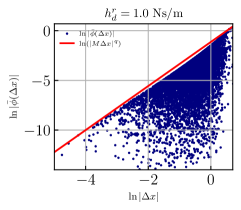
Refer to caption
Figure 4: Spring-damper-mass - plots of linearization error against |Δx|Δ𝑥|\Delta x| for 100001000010000 simulations showing the bound (red line).

The terminal radii are determined by performing 105superscript10510^{5} one-step simulations of the closed-loop system and estimating the linearization error bound. The linearization error of this system is independent of hdsubscript𝑑h_{d}, so the simulations were performed for only one of the disturbance realizations. After obtaining bound parameters Mr=0.3235subscript𝑀𝑟0.3235M_{r}=0.3235 and qr=2.2176subscript𝑞𝑟2.2176q_{r}=2.2176, the terminal radii were found to be cfr{0.8032, 0.8922, 0.6690}superscriptsubscript𝑐𝑓𝑟0.80320.89220.6690c_{f}^{r}\approx\{0.8032,\>0.8922,\>0.6690\}.

6.3 Simulation results

The simulations are done using JuMP v.0.21.10 [29] as the NLP modeler in a Julia [30] environment. The NLP solver used is IPOPT 3.13.4 [31], and the linear solver is HSL-MA57 [32] on a 2.6 GHz Intel Core-i7 with 16 GB memory.

An initial prediction horizon of N0=8subscript𝑁08N_{0}=8 is chosen with Nmin=2subscript𝑁min2N_{\text{min}}=2. The scenario tree is fully branched at each MPC iteration making a total of 6561 scenarios at the first iteration. Fig. 5 shows two sets of closed-loop simulations of the adaptive horizon multi-stage MPC that are done with initial conditions x0=[4, 4]subscript𝑥0superscript44topx_{0}=[-4,\>4]^{\top} mm\mathrm{m} (blue line) and [5.3, 2]superscript5.32top[5.3,\>2]^{\top} mm\mathrm{m} (black line). The state bounds are x1[10, 10]subscript𝑥11010x_{1}\in[-10,\>10] mm\mathrm{m} and x2[4, 10]subscript𝑥2410x_{2}\in[-4,\>10] m / s and the control input bounds are u|6.0N|𝑢6.0𝑁u\leq|6.0\>N|.

Refer to caption
Figure 5: Spring-damper-mass - simulation results from two initial conditions x0=[4, 4]subscript𝑥044x_{0}=[-4,\>4] (blue lines) and x0=[5.3, 2]subscript𝑥0superscript5.32topx_{0}=[5.3,\>2]^{\top} (black lines) showing the control performance of a fully branched adaptive horizon multi-stage MPC.

The system is controlled to its setpoint and the horizon length Nksubscript𝑁𝑘N_{k} is reduced as the setpoint is approached. Eventually, the Nksubscript𝑁𝑘N_{k} is reduced to 3 from 8 cutting the number of scenarios from 6561 to 27. Therefore, this example also demonstrates the advantage of the adaptive horizon method for computational cost savings in multi-stage MPC with a fully branched scenario tree.

6.4 Example 2 - Cooled CSTR

The rest of the numerical examples consider a robust horizon (i.e. no full branching), therefore recursive feasibility is not necessarily guaranteed (see Section 5.2). However, the aim is to compare the performances of the adaptive horizon multi-stage MPC (varying horizon lengths) with fixed horizon multi-stage MPC and to demonstrate the computational cost savings as a result of the adaptive horizon algorithm.

Consider the control of a CSTR with a cooling jacket example from [33]. The dynamics of the cooled CSTR are given by,

cA˙˙subscript𝑐𝐴\displaystyle\dot{c_{A}} =F(cA,0cA)k1cAk3cA2absent𝐹subscript𝑐𝐴0subscript𝑐𝐴subscript𝑘1subscript𝑐𝐴subscript𝑘3superscriptsubscript𝑐𝐴2\displaystyle=F(c_{A,0}-c_{A})-k_{1}c_{A}-k_{3}c_{A}^{2}
cB˙˙subscript𝑐𝐵\displaystyle\dot{c_{B}} =FcB+k1cAk2cBabsent𝐹subscript𝑐𝐵subscript𝑘1subscript𝑐𝐴subscript𝑘2subscript𝑐𝐵\displaystyle=-Fc_{B}+k_{1}c_{A}-k_{2}c_{B}
TR˙=F(TinTR)+kWARρcpVR(TJTR)k1cAΔHAB+k2cBΔHBC+k3cA2ΔHADρcp˙subscript𝑇𝑅𝐹subscript𝑇insubscript𝑇𝑅subscript𝑘𝑊subscript𝐴𝑅𝜌subscript𝑐𝑝subscript𝑉𝑅subscript𝑇𝐽subscript𝑇𝑅subscript𝑘1subscript𝑐𝐴Δsubscript𝐻𝐴𝐵subscript𝑘2subscript𝑐𝐵Δsubscript𝐻𝐵𝐶subscript𝑘3superscriptsubscript𝑐𝐴2Δsubscript𝐻𝐴𝐷𝜌subscript𝑐𝑝\displaystyle\begin{split}\dot{T_{R}}&=F(T_{\text{in}}-T_{R})+\frac{k_{W}A_{R}}{\rho c_{p}V_{R}}(T_{J}-T_{R})\\ &\qquad-\frac{k_{1}c_{A}\Delta H_{AB}+k_{2}c_{B}\Delta H_{BC}+k_{3}c_{A}^{2}\Delta H_{AD}}{\rho c_{p}}\end{split}
TJ˙˙subscript𝑇𝐽\displaystyle\dot{T_{J}} =1mJcp,J(QJ˙+kWAR(TRTJ))absent1subscript𝑚𝐽subscript𝑐𝑝𝐽˙subscript𝑄𝐽subscript𝑘𝑊subscript𝐴𝑅subscript𝑇𝑅subscript𝑇𝐽\displaystyle=\frac{1}{m_{J}c_{p,J}}(\dot{Q_{J}}+k_{W}A_{R}(T_{R}-T_{J}))

where reaction rates kisubscript𝑘𝑖k_{i} follow the Arrhenius law, ki=Aiexp(EiRTR)subscript𝑘𝑖subscript𝐴𝑖subscript𝐸𝑖𝑅subscript𝑇𝑅k_{i}=A_{i}\exp{\Big{(}\frac{-E_{i}}{RT_{R}}\Big{)}}.

Table 1: CSTR - Bounds on states and inputs
Variable Initial condition Minimum Maximum Unit
cAsubscript𝑐𝐴c_{A} 0.80.80.8 0.10.10.1 5.05.05.0 mol/lmoll\mathrm{mol}\mathrm{/}\mathrm{l}
cBsubscript𝑐𝐵c_{B} 0.50.50.5 0.10.10.1 5.95.95.9 mol/lmoll\mathrm{mol}\mathrm{/}\mathrm{l}
TRsubscript𝑇𝑅T_{R} 134.14134.14134.14 505050 140140140 \degreecelsius\degreecelsius\degreecelsius
TJsubscript𝑇𝐽T_{J} 134.0134.0134.0 505050 180180180 \degreecelsius\degreecelsius\degreecelsius
F𝐹F 18.8318.8318.83 0.00.00.0 353535 /habsenth\mathrm{/}\mathrm{h}
QJ˙˙subscript𝑄𝐽\dot{Q_{J}} 4495.74495.7-4495.7 85008500-8500 00 kJ/hkJh\mathrm{k}\mathrm{J}\mathrm{/}\mathrm{h}

The state variable vector x=[cA,cB,TR,TJ]𝑥superscriptsubscript𝑐𝐴subscript𝑐𝐵subscript𝑇𝑅subscript𝑇𝐽topx=[c_{A},\,c_{B},\,T_{R},\,T_{J}]^{\top} consists of the concentrations of A𝐴A and B𝐵B, reactor and coolant temperatures, respectively. The control inputs u𝑢u, are inlet flow per reactor volume F=Vin/VR𝐹subscript𝑉insubscript𝑉𝑅F=V_{\text{in}}/V_{R}, and cooling rate QJ˙˙subscript𝑄𝐽\dot{Q_{J}}.

The control objective is to regulate cBsubscript𝑐𝐵c_{B} at a desired setpoint. The system operates at two setpoints: cBset=0.5mol/superscriptsubscript𝑐𝐵set0.5molc_{B}^{\text{set}}=0.5\,\mathrm{mol}\mathrm{/}\ell, and cBset=0.7mol/superscriptsubscript𝑐𝐵set0.7molc_{B}^{\text{set}}=0.7\,\mathrm{mol}\mathrm{/}\ell. The activation energy E3=8560R±2.5%subscript𝐸3plus-or-minus8560𝑅percent2.5E_{3}=8560R\pm 2.5\% KK\mathrm{K} is the only uncertain parameter in the system. The stage cost is a setpoint tracking squared error of cBsubscript𝑐𝐵c_{B} plus control movement penalization terms ΔFi=FiFi1Δsubscript𝐹𝑖subscript𝐹𝑖subscript𝐹𝑖1\Delta F_{i}=F_{i}-F_{i-1} and ΔQJ˙k=QJ˙iQJ˙i1Δsubscript˙subscript𝑄𝐽𝑘subscript˙subscript𝑄𝐽𝑖subscript˙subscript𝑄𝐽𝑖1\Delta\dot{Q_{J}}_{k}=\dot{Q_{J}}_{i}-\dot{Q_{J}}_{i-1} given by k=(cBicBset)2+rΔ1ΔFi2+rΔ2ΔQJ˙i2subscript𝑘superscriptsubscriptsubscript𝑐𝐵𝑖superscriptsubscript𝑐𝐵set2subscriptsubscript𝑟Δ1Δsuperscriptsubscript𝐹𝑖2subscriptsubscript𝑟Δ2Δsuperscriptsubscript˙subscript𝑄𝐽𝑖2\ell_{k}=({c_{B}}_{i}-c_{B}^{\text{set}})^{2}+{r_{\Delta}}_{1}\Delta F_{i}^{2}+{r_{\Delta}}_{2}\Delta\dot{Q_{J}}_{i}^{2}. where the control penalties are rΔ1=105subscriptsubscript𝑟Δ1superscript105{r_{\Delta}}_{1}=10^{-5} and rΔ2=107subscriptsubscript𝑟Δ2superscript107{r_{\Delta}}_{2}=10^{-7}. Regularization terms are added to impose implicit references on the remaining states and strong convexity [24].

The initial prediction horizon is N0=40subscript𝑁040N_{0}=40. Terminal constraints are included for all the scenarios. The simulations are performed for NR=1, 2subscript𝑁𝑅12N_{R}=1,\,2. We sample three parameter realizations, such that when NR=2subscript𝑁𝑅2N_{R}=2 there are 9 scenarios as in Fig. 1.

6.4.1 Offline approximation of terminal ingredientd

To design a stabilizing LQR for each parametric realization, we use Q=I4𝑄subscript𝐼4Q=I_{4}, and R=diag([103 104])𝑅diagdelimited-[]superscript103superscript104R=\text{diag}([10^{-3}\,10^{-4}]). As outlined before, 105superscript10510^{5} one-step simulations are performed offline from random initial states to compute linearization error for each parametric realization and each operating point. Fig. 6 shows the plots of the linearization error against |Δx|Δ𝑥|\Delta x| for each parametric realization and each setpoint.

Refer to caption
Refer to caption
Figure 6: CSTR - plots of linearization error against |Δx|Δ𝑥|\Delta x| for 100001000010000 simulations for each parametric realization of E3subscript𝐸3E_{3}, at each setpoint cBset=0.5superscriptsubscript𝑐𝐵set0.5c_{B}^{\text{set}}=0.5 mol/\ell and 0.7 mol/\ell showing their bounds (red lines).

All the plots show an upper bound on the linearization error (red solid lines in Fig. 6) from which Mrsubscript𝑀𝑟M_{r} and qrsubscript𝑞𝑟q_{r} values are fitted. The terminal region radii for each parametric realization are obtained by evaluating (10) as shown in Table 2.

Table 2: CSTR - linearization error bounds and terminal radii
E3subscript𝐸3E_{3} ( K ) cBset=0.5superscriptsubscript𝑐𝐵set0.5c_{B}^{\text{set}}=0.5 mol/\ell cBset=0.7superscriptsubscript𝑐𝐵set0.7c_{B}^{\text{set}}=0.7 mol/\ell
Mrsubscript𝑀𝑟M_{r} qrsubscript𝑞𝑟q_{r} cfrsuperscriptsubscript𝑐𝑓𝑟c_{f}^{r} Mrsubscript𝑀𝑟M_{r} qrsubscript𝑞𝑟q_{r} cfrsuperscriptsubscript𝑐𝑓𝑟c_{f}^{r}
877487748774 0.620.620.62 2.02.02.0 0.14290.14290.1429 0.500.500.50 2.02.02.0 0.17180.17180.1718
856085608560 0.750.750.75 2.02.02.0 0.11590.11590.1159 0.620.620.62 2.02.02.0 0.13370.13370.1337
834683468346 1.121.121.12 2.02.02.0 0.07470.07470.0747 0.900.900.90 2.02.02.0 0.08460.08460.0846

6.4.2 Simulation results

A sample time of 18s18s18\,\mathrm{s} is used, and the process is simulated for 0.6h0.6h0.6\,\mathrm{h}. At the beginning cBset=0.5mol/superscriptsubscript𝑐𝐵set0.5molc_{B}^{\text{set}}=0.5\,\mathrm{mol}\mathrm{/}\ell and it changes to cBset=0.7mol/superscriptsubscript𝑐𝐵set0.7molc_{B}^{\text{set}}=0.7\,\mathrm{mol}\mathrm{/}\ell at tk=0.3hsubscript𝑡𝑘0.3ht_{k}=0.3\,\mathrm{h}. The uncertain parameter E3subscript𝐸3E_{3} is a random sequence of the sampled realizations. The control performance of the adaptive horizon multi-stage MPC is compared with the fixed horizon multi-stage MPC in this system. The value of Nmin=5subscript𝑁min5N_{\text{min}}=5 in the adaptive horizon multi-stage algorithm. Figs. 7 and 8 show closed-loop simulation results when NR=1, 2subscript𝑁𝑅12N_{R}=1,\,2, respectively.

Refer to caption
Figure 7: CSTR - Simulation results comparing the adaptive horizon multi-stage MPC with the fixed horizon multi-stage MPC when robust horizon NR=1subscript𝑁𝑅1N_{R}=1.
Refer to caption
Figure 8: CSTR - Simulation results comparing the adaptive horizon multi-stage MPC with the fixed horizon multi-stage MPC when robust horizon NR=2subscript𝑁𝑅2N_{R}=2.

The optimal input sequences and state trajectories for both controllers are nearly identical. The two controllers show similar performance in tracking changes in setpoint cBsetsuperscriptsubscript𝑐𝐵setc_{B}^{\text{set}}. This implies that the adaptive horizon algorithm does not affect the tracking performance of the multi-stage MPC.

The prediction horizon and total computation times per iteration for the two controllers when NR=1, 2subscript𝑁𝑅12N_{R}=1,\,2 are plotted in Figs. 9 and 10, respectively.
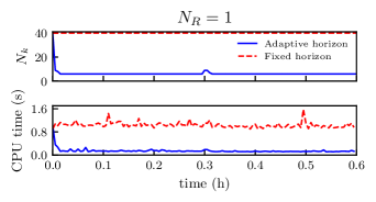
Refer to caption
Figure 9: CSTR - Simulation results comparing prediction horizons and computation times per iteration when robust horizon NR=1subscript𝑁𝑅1N_{R}=1.
Refer to caption
Figure 10: CSTR - Simulation results comparing prediction horizons and computation times per iteration when robust horizon NR=2subscript𝑁𝑅2N_{R}=2.

The adaptive horizon multi-stage MPC reduces the prediction horizon significantly, thus saving the computation time needed in each multi-stage MPC iteration. There is an 86%percent8686\% savings in CPU time on average from fixed horizon multi-stage MPC with NR=1subscript𝑁𝑅1N_{R}=1 by using the adaptive horizon multi-stage MPC. When NR=2subscript𝑁𝑅2N_{R}=2, there is also a 92%percent9292\% savings in CPU time on average. The regulatory performances of the two controllers are nearly identical but the prediction horizon and computation time are reduced significantly for the adaptive horizon multi-stage MPC.

6.5 Example 3 - Quad-tank system

The second example is from [34], on the control of a quad-tank system with four tanks. The liquid levels in the four tanks are described by the following set of differential equations:

x1˙˙subscript𝑥1\displaystyle\dot{x_{1}} =a1A12gx1+a3A12gx3+γ1A1u1absentsubscript𝑎1subscript𝐴12𝑔subscript𝑥1subscript𝑎3subscript𝐴12𝑔subscript𝑥3subscript𝛾1subscript𝐴1subscript𝑢1\displaystyle=-\frac{a_{1}}{A_{1}}\sqrt{2gx_{1}}+\frac{a_{3}}{A_{1}}\sqrt{2gx_{3}}+\frac{\gamma_{1}}{A_{1}}u_{1}
x2˙˙subscript𝑥2\displaystyle\dot{x_{2}} =a2A22gx2+a4A22gx4+γ2A2u2absentsubscript𝑎2subscript𝐴22𝑔subscript𝑥2subscript𝑎4subscript𝐴22𝑔subscript𝑥4subscript𝛾2subscript𝐴2subscript𝑢2\displaystyle=-\frac{a_{2}}{A_{2}}\sqrt{2gx_{2}}+\frac{a_{4}}{A_{2}}\sqrt{2gx_{4}}+\frac{\gamma_{2}}{A_{2}}u_{2}
x3˙˙subscript𝑥3\displaystyle\dot{x_{3}} =a3A32gx3+1γ2A3u2absentsubscript𝑎3subscript𝐴32𝑔subscript𝑥31subscript𝛾2subscript𝐴3subscript𝑢2\displaystyle=-\frac{a_{3}}{A_{3}}\sqrt{2gx_{3}}+\frac{1-\gamma_{2}}{A_{3}}u_{2}
x4˙˙subscript𝑥4\displaystyle\dot{x_{4}} =a4A42gx4+1γ1A4u1absentsubscript𝑎4subscript𝐴42𝑔subscript𝑥41subscript𝛾1subscript𝐴4subscript𝑢1\displaystyle=-\frac{a_{4}}{A_{4}}\sqrt{2gx_{4}}+\frac{1-\gamma_{1}}{A_{4}}u_{1}

where xisubscript𝑥𝑖x_{i} represents the liquid level in tank i𝑖i, uisubscript𝑢𝑖u_{i} is the flow rate of pump i𝑖i. The system has four states: x=[x1,x2,x3,x4]𝑥superscriptsubscript𝑥1subscript𝑥2subscript𝑥3subscript𝑥4topx=[x_{1},\,x_{2},\,x_{3},\,x_{4}]^{\top} and two control inputs: u=[u1,u2]𝑢superscriptsubscript𝑢1subscript𝑢2topu=[u_{1},\,u_{2}]^{\top}. Aisubscript𝐴𝑖A_{i} and aisubscript𝑎𝑖a_{i} are the cross sectional areas of the tank i𝑖i and its outlet, respectively. The valve coefficients γ1subscript𝛾1\gamma_{1} and γ2subscript𝛾2\gamma_{2} are the uncertain parameters of this system. The values of γ1,γ2=0.4±0.05subscript𝛾1subscript𝛾2plus-or-minus0.40.05\gamma_{1},\gamma_{2}=0.4\pm 0.05 and the system bounds are shown in Table 3.

Table 3: Quad-tank - Bounds on states and inputs
Variable Minimum Maximum Unit
x1subscript𝑥1x_{1} 7.57.57.5 28.028.028.0 cmcm\mathrm{c}\mathrm{m}
x2subscript𝑥2x_{2} 7.57.57.5 28.028.028.0 cmcm\mathrm{c}\mathrm{m}
x3subscript𝑥3x_{3} 14.214.214.2 28.028.028.0 cmcm\mathrm{c}\mathrm{m}
x4subscript𝑥4x_{4} 4.54.54.5 21.321.321.3 cmcm\mathrm{c}\mathrm{m}
u1subscript𝑢1u_{1} 0.00.00.0 60.060.060.0 m/sms\mathrm{m}\ell\mathrm{/}\mathrm{s}
u2subscript𝑢2u_{2} 0.00.00.0 60.060.060.0 m/sms\mathrm{m}\ell\mathrm{/}\mathrm{s}

The controller has a reference tracking objective, regulating the two levels in the lower tanks (tanks 1 and 2). The setpoints are x1set=x2set=14cmsuperscriptsubscript𝑥1setsuperscriptsubscript𝑥2set14cmx_{1}^{\text{set}}=x_{2}^{\text{set}}=14\,\mathrm{c}\mathrm{m}. We introduce predefined pulse changes in the state values at specific iterations to reset reference tracking as shown in Table 4.

Table 4: Pulse changes to state variables applied to the quad-tank system
k𝑘k x1subscript𝑥1x_{1} x2subscript𝑥2x_{2} x3subscript𝑥3x_{3} x4subscript𝑥4x_{4}
00 28 cmcm\mathrm{c}\mathrm{m} 28 cmcm\mathrm{c}\mathrm{m} 14.2 cmcm\mathrm{c}\mathrm{m} 21.3 cmcm\mathrm{c}\mathrm{m}
505050 28 cmcm\mathrm{c}\mathrm{m} 14 cmcm\mathrm{c}\mathrm{m} 28 cmcm\mathrm{c}\mathrm{m} 21.3 cmcm\mathrm{c}\mathrm{m}
100100100 28 cmcm\mathrm{c}\mathrm{m} 14 cmcm\mathrm{c}\mathrm{m} 14.2 cmcm\mathrm{c}\mathrm{m} 21.3 cmcm\mathrm{c}\mathrm{m}

The closed-loop multi-stage MPC simulations are run for 150 iterations with a sample time of 10s10s10\,\mathrm{s}. The stage cost function is given by: k=(x1ix1set)2+(x2ix2set)2+rΔ(Δu1i2+Δu2i2)subscript𝑘superscriptsubscriptsubscript𝑥1𝑖superscriptsubscript𝑥1set2superscriptsubscriptsubscript𝑥2𝑖superscriptsubscript𝑥2set2subscript𝑟ΔΔsuperscriptsubscriptsubscript𝑢1𝑖2Δsuperscriptsubscriptsubscript𝑢2𝑖2\ell_{k}=({x_{1}}_{i}-x_{1}^{\text{set}})^{2}+({x_{2}}_{i}-x_{2}^{\text{set}})^{2}+r_{\Delta}(\Delta{u_{1}}_{i}^{2}+\Delta{u_{2}}_{i}^{2}), where Δu1i=u1iu1i1Δsubscriptsubscript𝑢1𝑖subscriptsubscript𝑢1𝑖subscriptsubscript𝑢1𝑖1\Delta{u_{1}}_{i}={u_{1}}_{i}-{u_{1}}_{i-1} and Δu2i=u2iu2i1Δsubscriptsubscript𝑢2𝑖subscriptsubscript𝑢2𝑖subscriptsubscript𝑢2𝑖1\Delta{u_{2}}_{i}={u_{2}}_{i}-{u_{2}}_{i-1} are the control movement terms for the pump flow-rates that are penalized in the objective function with the penalty parameter rΔ=0.01subscript𝑟Δ0.01r_{\Delta}=0.01.

6.5.1 Offline approximation of terminal ingredients

LQR controller tuning Q=1.5I4𝑄1.5subscript𝐼4Q=1.5I_{4} and R=I2𝑅subscript𝐼2R=I_{2} are selected for the stabilizing controller for each parameter realization of γ1subscript𝛾1\gamma_{1} and γ2subscript𝛾2\gamma_{2}. As done previously, 105superscript10510^{5} one-step offline simulations from randomly sampled initial state values are performed for each parameter realization to compute the linearization error. The set 𝔻𝔻\mathbb{D} is obtained via grid-based sampling including the nominal and extreme parameter values only. A total of 9 parameter realizations are considered for the two uncertain parameters.
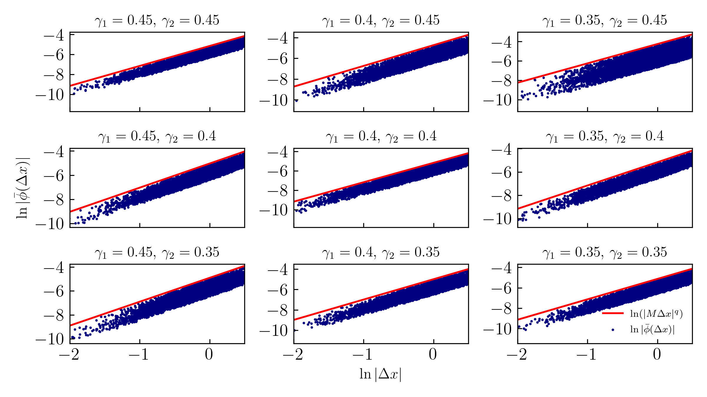
Refer to caption
Figure 11: Quad-tank - matrix of plots of linearization error against |Δx|Δ𝑥|\Delta x| of 10,0001000010,000 simulations for every uncertain parameter realization.

Fig. 11 is a matrix of linearization error plots from the one-step simulations with estimated upper bounds (red lines) for each uncertain parameter realization. The terminal radii for each parameter realization are computed using (10). The estimated linearization error bounds and terminal radii for each parameter realization are shown in Table 5.

Table 5: Quad-tank - linearization error bounds and terminal radii
[γ1;γ2]subscript𝛾1subscript𝛾2[\gamma_{1};\,\gamma_{2}] Mrsubscript𝑀𝑟M_{r} qrsubscript𝑞𝑟q_{r} cfrsuperscriptsubscript𝑐𝑓𝑟c_{f}^{r}
[0.45; 0.45]0.450.45[0.45;\,0.45] 0.00580.00580.0058 2.02.02.0 30.4330.4330.43
[0.40; 0.45]0.400.45[0.40;\,0.45] 0.00880.00880.0088 2.02.02.0 19.9919.9919.99
[0.35; 0.45]0.350.45[0.35;\,0.45] 0.01420.01420.0142 2.02.02.0 12.1212.1212.12
[0.45; 0.40]0.450.40[0.45;\,0.40] 0.00650.00650.0065 2.02.02.0 27.0427.0427.04
[0.40; 0.40]0.400.40[0.40;\,0.40] 0.00560.00560.0056 2.02.02.0 31.7731.7731.77
[0.35; 0.40]0.350.40[0.35;\,0.40] 0.00570.00570.0057 2.02.02.0 31.5731.5731.57
[0.45; 0.35]0.450.35[0.45;\,0.35] 0.00740.00740.0074 2.02.02.0 23.6923.6923.69
[0.40; 0.35]0.400.35[0.40;\,0.35] 0.00680.00680.0068 2.02.02.0 26.6326.6326.63
[0.35; 0.35]0.350.35[0.35;\,0.35] 0.00590.00590.0059 2.02.02.0 30.9730.9730.97

6.5.2 Simulation results

The parameters γ1subscript𝛾1\gamma_{1} and γ2subscript𝛾2\gamma_{2} have an uncertainty range of ±0.05plus-or-minus0.05\pm 0.05 about their nominal value. Similar to Example 2, the simulations are performed with a parameter sequence randomly sampled from {max, nom, min} values. Again, there are two simulation sets comparing the control performances of the adaptive horizon and fixed horizon multi-stage MPC when NR=1, 2subscript𝑁𝑅12N_{R}=1,\,2. Simulation results of the quad-tank system for the two controllers when NR=1, 2subscript𝑁𝑅12N_{R}=1,\,2 are plotted in Figs. 12 and 13, respectively.
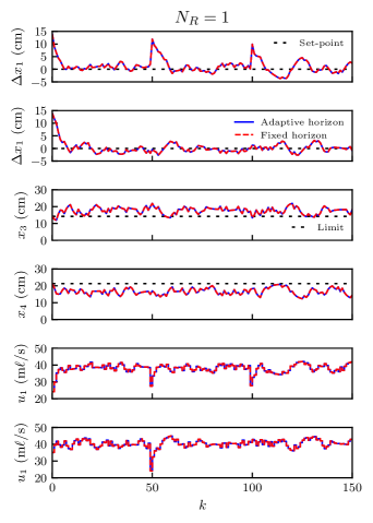
Refer to caption
Figure 12: Quad-tank - Simulation results comparing fixed horizon multi-stage and adaptive horizon multi-stage MPC with NR=1subscript𝑁𝑅1N_{R}=1.
Refer to caption
Figure 13: Quad-tank - Simulation results comparing fixed horizon multi-stage and adaptive horizon multi-stage MPC with NR=2subscript𝑁𝑅2N_{R}=2.

It is seen from the levels x1subscript𝑥1x_{1}, x2subscript𝑥2x_{2} that the setpoint tracking performance of the two controllers for both cases of NR=1, 2subscript𝑁𝑅12N_{R}=1,\,2 are again nearly identical. There are also no significant constraint violations in the bounds of x3subscript𝑥3x_{3}, x4subscript𝑥4x_{4} for both controllers. Therefore, there are no performance losses in both reference tracking and robustness of the multi-stage MPC by including the horizon update algorithm.

The prediction horizon and computation time per iteration for both controllers when NR=1, 2subscript𝑁𝑅12N_{R}=1,\,2 are plotted in Figs. 14 and 15, respectively.
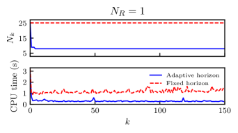
Refer to caption
Figure 14: Quad-tank - plot comparing prediction horizons and computation times at each iteration for ideal multi-stage and adaptive horizon multi-stage MPC with NR=1subscript𝑁𝑅1N_{R}=1.
Refer to caption
Figure 15: Quad-tank - plot comparing prediction horizons and computation times at each iteration for ideal multi-stage and adaptive horizon multi-stage MPC with NR=2subscript𝑁𝑅2N_{R}=2.

There is a reduction in the prediction horizon as the process approaches its setpoint. The horizon update algorithm is unaffected by the pulse changes in the tank levels. This is probably because the terminal radii values (see Table 5) are of the same order as the tank levels. Therefore the pulse changes do not displace the system far enough from the terminal region to cause a significant horizon increase. The average CPU time of the fixed horizon multi-stage MPC was significantly reduced by 74%percent7474\% with an adaptive horizon when NR=1subscript𝑁𝑅1N_{R}=1. Similarly, the CPU time reduction is 33%percent3333\% when NR=2subscript𝑁𝑅2N_{R}=2.

7 Conclusion

This paper adopts the existing adaptive horizon algorithm and extends it for multi-stage MPC to improve much-needed computational efficiency. First, the terminal costs and regions are computed independently for each uncertain parameter realization about their optimal steady states. We assume that a common terminal region exists for all uncertain parameter realizations, and the prediction horizon length is updated such that it is always reached.

The adaptive horizon framework is shown to be recursively feasible when the scenario tree is fully branched. Implementation of soft constraints may be used to avoid problem infeasibility in practice when the scenario tree is not fully branched, but then robust constraint satisfaction is not guaranteed. The ISpS stability of the fixed horizon multi-stage MPC is retained in this framework by assuming negligible linear control error inside the common terminal region.

Simulation results on three examples demonstrate an effective reduction in the prediction horizon and computational delay, provided the system progressively approaches its setpoint, and that it is not significantly disturbed away from it. Future avenues for this work include handling economic costs, and the use of parametric sensitivities for both horizon and critical scenario updates to further reduce computation time.

CRediT Author Statement

Zawadi Mdoe: Conceptualization, Methodology, Software, Investigation, Writing - original draft, Writing - review & editing, Visualization. Dinesh Krishnamoorthy: Conceptualization, Methodology, Writing - review & editing. Johannes Jäschke: Conceptualization, Methodology, Writing - original draft, Writing - review & editing, Supervision.

Declaration of Competing Interest

The authors declare that they have no known competing financial interests or personal relationships that could have appeared to influence the work reported in this paper.

References

  • Rawlings et al. [2017] J. B. Rawlings, D. Q. Mayne, M. Diehl, Model predictive control: theory, computation, and design, volume 2, Nob Hill Publishing Madison, WI, 2017.
  • Murty and Kabadi [1985] K. G. Murty, S. N. Kabadi, Some NP-complete problems in quadratic and nonlinear programming, Technical Report, 1985.
  • Scokaert and Mayne [1998] P. O. Scokaert, D. Q. Mayne, Min-max feedback model predictive control for constrained linear systems, IEEE Transactions on Automatic control 43 (1998) 1136–1142.
  • Lucia and Engell [2013] S. Lucia, S. Engell, Robust nonlinear model predictive control of a batch bioreactor using multi-stage stochastic programming, in: 2013 European Control Conference (ECC), IEEE, 2013, pp. 4124–4129.
  • de la Pena et al. [2006] D. M. de la Pena, T. Alamo, A. Bemporad, E. F. Camacho, Feedback min-max model predictive control based on a quadratic cost function, in: 2006 American Control Conference, IEEE, 2006, pp. 6–pp.
  • Lucia et al. [2013] S. Lucia, T. Finkler, S. Engell, Multi-stage nonlinear model predictive control applied to a semi-batch polymerization reactor under uncertainty, Journal of Process Control 23 (2013) 1306–1319.
  • Krener [2018] A. J. Krener, Adaptive horizon model predictive control, IFAC-PapersOnLine 51 (2018) 31–36.
  • Krener [2019] A. J. Krener, Adaptive Horizon Model Predictive Control and Al’brekht’s Method, Springer London, London, 2019, pp. 1–14. URL: https://doi.org/10.1007/978-1-4471-5102-9_100071-1. doi:10.1007/978-1-4471-5102-9_100071-1.
  • Griffith et al. [2018] D. W. Griffith, L. T. Biegler, S. C. Patwardhan, Robustly stable adaptive horizon nonlinear model predictive control, Journal of Process Control 70 (2018) 109–122.
  • Mdoe et al. [2021] Z. Mdoe, D. Krishnamoorthy, J. Jaschke, Adaptive horizon multistage nonlinear model predictive control, in: 2021 American Control Conference (ACC), IEEE, 2021, pp. 2088–2093.
  • De Nicolao et al. [1996] G. De Nicolao, L. Magni, R. Scattolini, On the robustness of receding-horizon control with terminal constraints, IEEE Transactions on Automatic Control 41 (1996) 451–453.
  • Pannocchia et al. [2011] G. Pannocchia, J. B. Rawlings, S. J. Wright, Conditions under which suboptimal nonlinear mpc is inherently robust, Systems & Control Letters 60 (2011) 747–755.
  • Yu et al. [2014] S. Yu, M. Reble, H. Chen, F. Allgöwer, Inherent robustness properties of quasi-infinite horizon nonlinear model predictive control, Automatica 50 (2014) 2269–2280.
  • Allan et al. [2017] D. A. Allan, C. N. Bates, M. J. Risbeck, J. B. Rawlings, On the inherent robustness of optimal and suboptimal nonlinear mpc, Systems & Control Letters 106 (2017) 68–78.
  • Shekhar [2012] R. C. Shekhar, Variable horizon model predictive control: robustness and optimality, Ph.D. thesis, University of Cambridge, 2012.
  • Krishnamoorthy et al. [2020] D. Krishnamoorthy, L. T. Biegler, J. Jäschke, Adaptive horizon economic nonlinear model predictive control, Journal of Process Control 92 (2020) 108–118.
  • Chen and Allgöwer [1998] H. Chen, F. Allgöwer, A quasi-infinite horizon nonlinear model predictive control scheme with guaranteed stability, Automatica 34 (1998) 1205–1217.
  • Nocedal and Wright [2006] J. Nocedal, S. Wright, Numerical optimization, Springer Science & Business Media, 2006.
  • Fiacco [1976] A. V. Fiacco, Sensitivity analysis for nonlinear programming using penalty methods, Mathematical programming 10 (1976) 287–311.
  • Sontag [1989] E. Sontag, Smooth stabilization implies coprime factorization, IEEE Transactions on Automatic Control 34 (1989) 435–443. doi:10.1109/9.28018.
  • Sontag and Wang [1996] E. D. Sontag, Y. Wang, New characterizations of input-to-state stability, IEEE transactions on automatic control 41 (1996) 1283–1294.
  • Limón et al. [2006] D. Limón, T. Alamo, F. Salas, E. F. Camacho, Input to state stability of min–max mpc controllers for nonlinear systems with bounded uncertainties, Automatica 42 (2006) 797–803.
  • Ralph and Dempe [1995] D. Ralph, S. Dempe, Directional derivatives of the solution of a parametric nonlinear program, Mathematical programming 70 (1995) 159–172.
  • Jäschke et al. [2014] J. Jäschke, X. Yang, L. T. Biegler, Fast economic model predictive control based on nlp-sensitivities, Journal of Process Control 24 (2014) 1260–1272.
  • Maiworm et al. [2015] M. Maiworm, T. Bäthge, R. Findeisen, Scenario-based model predictive control: Recursive feasibility and stability, IFAC-PapersOnLine 48 (2015) 50–56.
  • Lucia et al. [2020] S. Lucia, S. Subramanian, D. Limon, S. Engell, Stability properties of multi-stage nonlinear model predictive control, Systems & Control Letters 143 (2020) 104743.
  • Thombre et al. [2021] M. Thombre, Z. J. Yu, J. Jäschke, L. T. Biegler, Sensitivity-assisted multistage nonlinear model predictive control: Robustness, stability and computational efficiency, Computers & Chemical Engineering 148 (2021) 107269.
  • Raimondo et al. [2009] D. M. Raimondo, D. Limon, M. Lazar, L. Magni, E. F. ndez Camacho, Min-max model predictive control of nonlinear systems: A unifying overview on stability, European Journal of Control 15 (2009) 5–21.
  • Dunning et al. [2017] I. Dunning, J. Huchette, M. Lubin, Jump: A modeling language for mathematical optimization, SIAM Review 59 (2017) 295–320. doi:10.1137/15M1020575.
  • Bezanson et al. [2017] J. Bezanson, A. Edelman, S. Karpinski, V. B. Shah, Julia: A fresh approach to numerical computing, SIAM Review 59 (2017) 65–98. URL: https://doi.org/10.1137/141000671. doi:10.1137/141000671. arXiv:https://doi.org/10.1137/141000671.
  • Wächter and Biegler [2006] A. Wächter, L. T. Biegler, On the implementation of an interior-point filter line-search algorithm for large-scale nonlinear programming, Mathematical programming 106 (2006) 25–57.
  • STFC Rutherford Appleton Laboratory [2019] STFC Rutherford Appleton Laboratory, HSL. A collection of Fortran codes for large-scale scientific computation, http://www.hsl.rl.ac.uk (2019).
  • Klatt and Engell [1998] K.-U. Klatt, S. Engell, Gain-scheduling trajectory control of a continuous stirred tank reactor, Computers & Chemical Engineering 22 (1998) 491–502.
  • Raff et al. [2006] T. Raff, S. Huber, Z. K. Nagy, F. Allgower, Nonlinear model predictive control of a four tank system: An experimental stability study, in: 2006 IEEE Conference on Computer Aided Control System Design, 2006 IEEE International Conference on Control Applications, 2006 IEEE International Symposium on Intelligent Control, IEEE, 2006, pp. 237–242.