SimFBO: Towards Simple, Flexible and Communication-efficient Federated Bilevel Learning

Abstract

Federated bilevel optimization (FBO) has shown great potential recently in machine learning and edge computing due to the emerging nested optimization structure in meta-learning, fine-tuning, hyperparameter tuning, etc. However, existing FBO algorithms often involve complicated computations and require multiple sub-loops per iteration, each of which contains a number of communication rounds. In this paper, we propose a simple and flexible FBO framework named SimFBO, which is easy to implement without sub-loops, and includes a generalized server-side aggregation and update for improving communication efficiency. We further propose System-level heterogeneity robust FBO (ShroFBO) as a variant of SimFBO with stronger resilience to heterogeneous local computation. We show that SimFBO and ShroFBO provably achieve a linear convergence speedup with partial client participation and client sampling without replacement, as well as improved sample and communication complexities. Experiments demonstrate the effectiveness of the proposed methods over existing FBO algorithms.

1 Introduction

Recent years have witnessed significant progress in a variety of emerging areas including meta-learning and fine-tuning [11, 52], automated hyperparameter optimization [13, 10], reinforcement learning [31, 21], fair batch selection in machine learning [54], adversarial learning [76, 40], AI-aware communication networks [27], fairness-aware federated learning [75], etc. These problems share a common nested optimization structure, and have inspired intensive study on the theory and algorithmic development of bilevel optimization. Prior efforts have been taken mainly on the single-machine scenario. However, in modern machine learning applications, data privacy has emerged as a critical concern in centralized training, and the data often exhibit an inherently distributed nature [70]. This highlights the importance of recent research and attention on federated bilevel optimization, and has inspired many emerging applications including but not limited to federated meta-learning [9], hyperparameter tuning for federated learning [25], resource allocation over communication networks [27] and graph-aided federated learning [71], adversarial robustness on edge computing [46], etc. In general, the federated bilevel optimization problem takes the following mathematical formulation.

$$\min_{x\in\mathbb{R}^{p}}\Phi(x)=F\big{(}x,y^{*}(x)\big{)}:=\sum_{i=1}^{n}p_{i}f_{i}(x,y^{*}(x))=\sum_{i=1}^{n}p_{i}\mathbb{E}_{\xi}\Big{[}f_{i}\big{(}x,y^{*}(x);\xi_{i}\big{)}\Big{]}$$

$$\;\;\mbox{s.t.}\;y^{*}(x)=\operatorname*{arg\,min}_{y\in\mathbb{R}^{q}}G(x,y):=\sum_{i=1}^{n}p_{i}g_{i}(x,y)=\sum_{i=1}^{n}p_{i}\mathbb{E}_{\zeta}\big{[}g_{i}(x,y;\zeta_{i})\big{]}$$ (1)

where $n$ is the total number of clients, the outer- and inner-functions $f_{i}(x,y)$ and $g_{i}(x,y)$ for each client $i$ take the expectation forms w.r.t. the random variables $\xi_{i}$ and $\zeta_{i}$, and are jointly continuously differentiable. However, efficiently solving the federated problem in section 1 suffers from several main challenges posed by the federated hypergradient (i.e., $\nabla\Phi(x)$) computation that contains the second-order global Hessian-inverse matrix, the lower- and upper-level data and system-level heterogeneity, and the nested optimization structure. To address these issues, [25, 65, 24, 22] proposed approximate implicit differentiation (AID)-based federated bilevel algorithms, which applied the idea of non-federated AID-based estimate in [15] to the federated setting, and involve two sub-loops for estimating the global lower-level solution $y^{*}(x)$ and the Hessian-inverse-vector product, respectively. [69] then proposed AggITD by leveraging the idea of iterative differentiation, which improved the communication efficiency of AID-based approaches by synthesizing the lower-level optimization and the hypergradient computation into the same communication sub-loop. However, some limitations still remain in these approaches.

• First, the sub-loops, each with a large number of communication rounds, often compute products of a series of matrix-vector products, and hence can complicate the implementation and increase the communication cost.

• Second, the practical client sampling without replacement has not been studied in these methods due to challenges posed by the nested structure of AID- and ITD-based federated hypergradient estimators.

• Third, as observed in the single-level federated learning [67], in the presence of heterogeneous system capabilities such as diverse computing power and storage, clients can take a variable number of local updates or use different local optimizers, which may make these FBO algorithms converge to the stationary point of a different objective.

Figure 1: Comparison of AID-based federated hypergradient estimation (FHE) in FedNest [65] (left), ITD-based FHE in AggITD [69] (middle) and our proposed SimFBO (right) at each iteration.

1.1 Our Contributions

In this paper, we propose a communication-efficient federated bilevel method named SimFBO, which is simple to implement without sub-loops, flexible with a generalized server-side update, and resilient to system-level heterogeneity. Our specific contributions are summarized below.

A simple and flexible implementation. As illustrated in Figure 1, differently from AID- and ITD-based approaches that contain multiple sub-loops of communication rounds at each iteration, our proposed SimFBO is simpler with a single communication round per iteration, in which three variables $y,x$ and $v$ are updated simultaneously for optimizing the lower- and upper-level problems, and approximating the Hessian-inverse-vector product. SimFBO also includes a generalized server-side update on $x,y,v$, which accommodates the client sampling without replacement, and allows for a flexible aggregation to improve the communication efficiency.

Resilient server-side updates to system-level heterogeneity. In the presence of heterogeneous local computation, we show that the naive server-side aggregation can lead to the convergence to a stationary point of a different objective. To this end, we propose System-level heterogeneity robust FBO (ShroFBO) building on a normalized version of the generalized server-side update with correction, which provably converges to a stationary point of the original objective.

Convergence analysis and improved complexity. As shown in Table 1, our SimFBO and ShroFBO both achieve a sample complexity (i.e., the number of samples needed to reach an $\epsilon$-accurate stationary point) of $\mathcal{O}(\epsilon^{-2}P^{-1})$, which matches the best result obtained by FedMBO [24] but under a more practical client sampling without replacement. Moreover, SimFBO and ShroFBO both achieve the best communication complexity (i.e., the number of communication rounds to reach an $\epsilon$-accurate stationary point) of $\mathcal{O}(\epsilon^{-1})$, which improves those of other methods by an order of $\epsilon^{-1/2}$. Technically, we develop novel analysis in characterizing the client drifts by the three variables, bounding the per-iteration progress in the global $y$ and $v$ updates, and proving the smoothness and bounded variance in local $v$ updates via induction, which may be of independent interest.

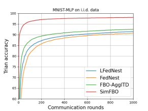
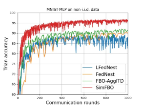
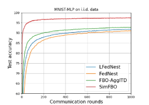
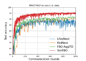
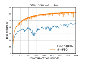
Superior performance in practice. In the experiments, the proposed SimFBO method significantly improves over existing strong federated bilevel baselines such as AggITD, FedNest and LFedNest in both the i.i.d. and non-i.i.d. settings. We also validate the better performance of ShroFBO in the presence of heterogeneous local computation due to the resilient server-side updates.

Algorithm	System-level heterogeneity	Partial participation	Without replacement	Linear speedup	Samples complexity	Communication complexity
FedNest [65]	✗	✗	✗	✗	$\mathcal{O}(\epsilon^{-2})$	$\mathcal{O}(\epsilon^{-2})$
FBO-AggITD [69]	✗	✗	✗	✗	$\mathcal{O}(\epsilon^{-2})$	$\mathcal{O}(\epsilon^{-2})$
FedBiO [36]	✗	✗	✗	✓	$\mathcal{O}(\epsilon^{-2.5}n^{-1})$	$\mathcal{O}(\epsilon^{-1.5})$
FedMBO [24]	✗	✓	✗	✓	$\mathcal{O}(\epsilon^{-2}P^{-1})$	$\mathcal{O}(\epsilon^{-2})$
SimFBO (this paper)	✗	✓	✓	✓	$\mathcal{O}(\epsilon^{-2}P^{-1})$	$\mathcal{O}(\epsilon^{-1})$
ShroFBO (this paper)	✓	✓	✓	✓	$\mathcal{O}(\epsilon^{-2}P^{-1})$	$\mathcal{O}(\epsilon^{-1})$

Table 1: Comparison of different federated bilevel algorithms in the setting with heterogeneous data. We do not include the methods with momentum-based acceleration for a fair comparison. $P\leq n$ is the number of sampled clients in each communication round.

2 SimFBO: A Simple and Flexible Framework

2.1 Preliminary: Federated Hypergradient Computation

The biggest challenge in FBO is to compute the federated hypergradient $\nabla\Phi(x)$ due to the implicit and complex dependence of $y^{*}(x)$ on $x$. Under suitable assumptions and using the implicit function theorem in [18], it has been shown that the $\nabla\Phi(x)$ takes the form of

$$\nabla\Phi(x) =\sum_{i=1}^{n}p_{i}\nabla_{x}f_{i}(x,y^{*})-\nabla_{xy}^{2}G(x,y^{*})\big{[}\nabla_{yy}^{2}G(x,y^{*})\big{]}^{-1}\sum_{i=1}^{n}p_{i}\nabla_{y}f_{i}(x,y^{*})$$

which poses several computational challenges in the federated setting. First, the second term at the right-hand side contains three global components in a nonlinear manner, and hence the direct aggregation of local hypergradients given by

$$\sum_{i=1}^{n}p_{i}\big{(}\nabla_{x}f_{i}(x,y^{*})-\nabla_{xy}^{2}g_{i}(x,y^{*})\big{[}\nabla_{yy}^{2}g_{i}(x,y^{*})\big{]}^{-1}\nabla_{y}f_{i}(x,y^{*})\big{)}$$

is a biased estimation of $\nabla\Phi(x)$ due to the client drift. Second, it is infeasible to compute, store and communicate the second-order Hessian-inverse and Jacobian matrices due to the limited computing and communication resource. Although various AID- and ITD-based approaches have been proposed to address these challenges, they still suffer from several limitations (as we point out in the introduction) such as complicated implementation, high communication cost, lack of client sampling without replacement, and vulnerability to the system-level heterogeneity. To this end, we propose a simple, flexible and communication-efficient FBO framework named SimFBO in this section.

2.2 Federated Hypergradient Surrogate

To estimate the federated hypergradient efficiently, we use the surrogate $\bar{\nabla}F(x,y,v)=\nabla_{x}F(x,y)-\nabla_{xy}^{2}G(x,y)v$, where $v\in R^{d_{y}}$ is an auxiliary vector. Then, it suffices to find $y$ and $v$ as efficient estimates of the solutions to the global lower-level problem and the global linear system (LS) $\nabla_{yy}^{2}G(x,y)v=\nabla_{y}F(x,y)$ that is equivalent to solving following quadratic programming.

$$\min_{v}\;R(x,y,v) =\frac{1}{2}v^{T}\nabla_{yy}^{2}G(x,y)v-v^{T}\nabla_{y}F(x,y)$$

$$=\sum_{i=1}^{n}p_{i}\big{(}\underbrace{\frac{1}{2}v^{T}\nabla_{yy}^{2}g_{i}(x,y)v-v^{T}\nabla_{y}f_{i}(x,y)}_{R_{i}(x,y,v)}\big{)},$$ (2)

where $R_{i}(x,y,v)$ can be regarded as the loss function of client $i$ for solving this global LS problem. Based on this surrogate, we next describe the proposed SimFBO framework.

2.3 Simple Local and Server-side Aggregations and Updates

Simple local update. Differently from FedNest [65] and AggITD [69] that perform the lower-level optimization, the federated hypergradient estimation and the upper-level update alternatively in different communication sub-loops, our SimFBO conducts the simple updates on all these three procedures simultaneously in each communication round. In specific, each communication round $t$ first selects a subset $C^{(t)}$ of participating clients without replacement. Then, each active client $i\in C^{(t)}$ updates three variables $y,v,x$ at $k^{th}$ local iteration simultaneously as

$$\begin{pmatrix}y_{i}^{(t,k+1)}\vspace{0.2cm}\\ v_{i}^{(t,k+1)}\vspace{0.2cm}\\ x_{i}^{(t,k+1)}\end{pmatrix}\leftarrow\begin{pmatrix}y_{i}^{(t,k)}\vspace{0.2cm}\\ v_{i}^{(t,k)}\vspace{0.2cm}\\ x_{i}^{(t,k)}\end{pmatrix}-a_{i}^{(t,k)}\begin{pmatrix}\eta_{y}\nabla_{y}g_{i}\big{(}x_{i}^{(t,k)},y_{i}^{(t,k)};\zeta_{i}^{(t,k)}\big{)}\vspace{0.2cm}\\ \eta_{v}\nabla_{v}R_{i}\big{(}x_{i}^{(t,k)},y_{i}^{(t,k)},v_{i}^{(t,k)};\psi_{i}^{(t,k)}\big{)}\vspace{0.2cm}\\ \eta_{x}\bar{\nabla}f_{i}\big{(}x_{i}^{(t,k)},y_{i}^{(t,k)},v_{i}^{(t,k)};\xi_{i}^{(t,k)}\big{)}\end{pmatrix}$$ (3)

where $\eta_{y}$, $\eta_{v}$, $\eta_{x}$ correspond to the local stepsizes, $a_{i}^{(t,k)}$ is a client-specific coefficient to increase the flexibility of the framework, $\zeta_{i}^{(t,k)}$, $\psi_{i}^{(t,k)}$, $\xi_{i}^{(t,k)}$ are independent samples, and the local hypergradient estimate takes the form of $\bar{\nabla}f_{i}\big{(}x,y,v;\xi\big{)}=\nabla_{x}f_{i}\big{(}x,y;\xi\big{)}-\nabla_{xy}^{2}g_{i}\big{(}x,y;\xi\big{)}v_{i}.$ The variables $y,v$ and $x$ in eq. 3, which optimize the lower-level problem, the LS problem and the upper-level problem, are updated with totally $\tau_{i}^{(t)}$ local steps. Note that the updates in eq. 3 also allow for parallel computation on $x,v$ and $y$ locally.

Local and server-side aggregation. After completing all local updates, the next step is to aggregate such local information on both the client and server sides. As shown in section 2.3, each participating client $i\in C^{(t)}$ aggregates all the local gradients, and then communicate the aggregations $q_{y,i}^{(t)},q_{v,i}^{(t)}$ and $q_{x,i}^{(t)}$ to the server. Then, on the server side, such local information is further aggregated to be $q_{y}^{(t)},q_{v}^{(t)}$ and $q_{x}^{(t)}$, which will be used for a subsequent generalized server-side update.

$$q_{y}^{(t)}=\sum_{i\in C^{(t)}}\widetilde{p}_{i}q_{y,i}^{(t)}= \sum_{i\in C^{(t)}}\widetilde{p}_{i}\sum_{k=0}^{\tau_{i}-1}a_{i}^{(t,k)}\nabla_{y}g_{i}\big{(}x_{i}^{(t,k)},y_{i}^{(t,k)};\zeta_{i}^{(t,k)}\big{)},$$

$$q_{v}^{(t)}=\sum_{i\in C^{(t)}}\widetilde{p}_{i}q_{v,i}^{(t)}= \sum_{i\in C^{(t)}}\widetilde{p}_{i}\sum_{k=0}^{\tau_{i}-1}a_{i}^{(t,k)}\nabla_{v}R_{i}\big{(}x_{i}^{(t,k)},y_{i}^{(t,k)}v_{i}^{(t,k)};\psi_{i}^{(t,k)}\big{)},$$

$$\underbrace{q_{x}^{(t)}=\sum_{i\in C^{(t)}}\widetilde{p}_{i}q_{x,i}^{(t)}}_{\text{Server aggregation}}= \sum_{i\in C^{(t)}}\widetilde{p}_{i}\underbrace{\sum_{k=0}^{\tau_{i}-1}a_{i}^{(t,k)}\bar{\nabla}f_{i}\big{(}x_{i}^{(t,k)},y_{i}^{(t,k)},v_{i}^{(t,k)};\xi_{i}^{(t,k)}\big{)}}_{\text{Local aggregation}},$$ (4)

where $\widetilde{p}_{i}:=\frac{n}{|C^{(t)}|}p_{i}$ is the effective weight of client $i\in C^{(t)}$ among all participating clients such that $\mathbb{E}(\sum_{i\in C^{(t)}}\widetilde{p}_{i})=1$. Note that in section 2.3, the local aggregation $q_{y,i}^{(t)}$ (similarly for $v$ and $x$) can be regarded as a linear combination of all local stochastic gradients, and hence covers a variety of local optimizers such as stochastic gradient descent, momentum-based gradient, variance reduction by choosing different coefficients $a^{(t,k)}_{i}$ for $i\in C^{(t)}$. This substantially enhances the flexibility of the proposed framework.

Algorithm 1 SimFBO and ShroFBO

1:  Input: initialization $\bm{x}^{(0)}$,$\bm{y}^{(0)}$, number of communication rounds $T$, learning rates: client $\{\eta_{y},\eta_{v},\eta_{x}\}$, server: $\{\gamma_{y},\gamma_{v},\gamma_{x}\}$, local update rounds: $\{\tau_{i}^{(t)}\}$

2:  for $t=0,1,2,...,T$ do

3:     for $i\in C^{(t)}$ in parallel do

4:        $y_{i}^{(t,0)}=y^{(t)}$, $v_{i}^{(t,0)}=v^{(t)}$, $x_{i}^{(t,0)}=x^{(t)}$

5:        for $k=0,1,2,...,\tau_{i}^{(t)}-1$ do

6:           Locally update $y_{i}^{(t,k)}$, $v_{i}^{(t,k)}$ and $x_{i}^{(t,k)}$ simultaneously via eq. 3

7:        end for

8:        Client $i$ locally aggregates gradients to compute $q_{y,i}^{(t)}$, $q_{v,i}^{(t)}$, $q_{x,i}^{(t)}$ via section 2.3

9:        Client $i$ locally aggregates gradients to compute $h_{y,i}^{(t)}$, $h_{v,i}^{(t)}$, $h_{x,i}^{(t)}$ defined in eq. 6

10:     end for

11:     Client $i\in C^{(t)}$ communicate $\{h_{y,i}^{(t)},h_{v,i}^{(t)},h_{x,i}^{(t)}\}$ to the server

12:     Server aggregates local estimators to compute $\{q_{y}^{(t)},q_{v}^{(t)},q_{x}^{(t)}\}$ using section 2.3

13:     Server aggregates local estimators to compute $\{h_{y}^{(t)},h_{v}^{(t)},h_{x}^{(t)}\}$ using eq. 7

14:     Server updates using eq. 5

15:     Server updates using eq. 8

16:  end for

Server-side updates. Based on the aggregated gradients $q_{y}^{(t)},q_{v}^{(t)}$ and $q_{x}^{(t)}$, we then perform server-level gradient-based updates on variables $x,v$ and $y$ simultaneously as

$$y^{(t+1)}=y^{(t)}-\gamma_{y}q_{y}^{(t)},\;\;v^{(t+1)}=\mathcal{P}_{r}\big{(}v^{(t)}-\gamma_{v}q_{v}^{(t)}\big{)},\;\;x^{(t+1)}=x^{(t)}-\gamma_{x}q_{x}^{(t)},$$ (5)

where $\gamma_{y}$, $\gamma_{v}$ and $\gamma_{x}$ are server-side updating stepsizes for $y$, $v$, $x$ and $\mathcal{P}_{r}(v):=\min\big{\{}1,\frac{r}{\|v\|}\big{\}}v$ is a simple projection on a bounded ball with a radius of $r$. There are a few remarks about the updates in eq. 5. First, in contrast to existing FBO algorithms such as [65, 69], our introduced server-side updates leverage not only the client-side stepsizes $\eta_{y},\eta_{v},\eta_{x}$, but also the server-side stepsizes $\gamma_{y},\gamma_{v}$ and $\gamma_{x}$. This generalized two-learning-rate paradigm can provide more algorithmic and theoretical flexibility, and provides improved communication efficiency in practice and in theory. Second, the projection $\mathcal{P}_{r}(\cdot)$ serves as an important step to ensure the boundedness of variable $v^{(t)}$, and hence guarantee the smoothness of the global LS problem and the boundedness of the estimation variance in $v$ and $x$ updates, both of which are crucial and necessary in the final convergence analysis. Note that we do not impose such projection on the local $v_{i}^{(t,k)}$ variables because we can prove via induction that they are bounded given the boundedness of $v^{(t)}$ (see Proposition 1).

2.4 Resilient Server-side Updates against System-level Heterogeneity

Limitations under system-level heterogeneity. When clients have heterogeneous computing and storing capabilities (e.g., computer server v.s. phone in edge computing), an unequal number of local updates are often performed such that the global solution can be biased toward those of the clients with much more local steps or stronger optimizers. As observed in [67], this heterogeneity can deviate the iterates to minimize a different objective function. To explain this mismatch phenomenon, inspired by [57], we rewrite the server-side update on $x$ (similarly for $v$ and $y$) in section 2.3 as

$$q_{x}^{(t)} =\sum_{i=1}^{n}p_{i}q_{x,i}^{(t,k)}=\underbrace{\Big{(}\sum_{j=1}^{n}p_{j}\|a_{j}^{(t)}\|_{1}\Big{)}}_{\rho^{(t)}}\sum_{i=1}^{n}\underbrace{\frac{p_{i}\|a_{i}^{(t)}\|_{1}}{\sum_{j=1}^{n}p_{j}\|a_{j}^{(t)}\|_{1}}}_{w_{i}}\underbrace{\frac{q_{x,i}^{(t)}}{\|a_{i}^{(t)}\|_{1}}}_{h_{x,i}^{(t)}}.$$ (6)

where $a_{i}^{(t)}=\big{[}a_{i}^{(t,0)},...,a_{i}^{(t,\tau_{i}^{(t)}-1)}\big{]}^{T}$ collects all local coefficients of client $i$, and $h_{x,i}^{(t)}$ normalizes the aggregated gradient $q_{x,i}^{(t)}$ by $1/\|a_{i}^{(t)}\|_{1}$ such that $\|h_{x,i}^{(t)}\|$ does not grow with the increasing of $\tau_{i}^{(t)}$. Although such normalization can help to mitigate the system-level heterogeneity, the effective weight $w_{i}$ can deviate from the true weight $p_{i}$ of the original objective in section 1, and the iterates converge to the stationary point of a different objective that replaces all $p_{i}$ by $w_{i}$ in section 1 (see Theorem 1).

System-level heterogeneity robust FBO (ShroFBO). To address this convergence issue, we then propose a new method named ShroFBO with stronger resilience to such heterogeneity. Motivated by the normalized reformulation in eq. 6, ShroFBO adopts a different server-side aggregation as

$$h_{y}^{(t)}=\sum_{i\in C^{(t)}}\widetilde{p}_{i}h_{y,i}^{(t)},\quad h_{v}^{(t)}=\sum_{i\in C^{(t)}}\widetilde{p}_{i}h_{v,i}^{(t)},\quad h_{x}^{(t)}=\sum_{i\in C^{(t)}}\widetilde{p}_{i}h_{x,i}^{(t)},$$ (7)

where $\widetilde{p}_{i}:=\frac{n}{|C^{(t)}|}p_{i}$ and $h_{y,i}^{(t)},h_{v,i}^{(t)},h_{x,i}^{(t)}$ are the normalized local aggregations defined in eq. 6. Accordingly, the server-side updates become

$$y^{(t+1)}=y^{(t)}-\rho^{(t)}\gamma_{y}h_{y}^{(t)},\;\;v^{(t+1)}=\mathcal{P}_{r}\big{(}v^{(t)}-\rho^{(t)}\gamma_{v}h_{v}^{(t)}\big{)},\;\;x^{(t+1)}=x^{(t)}-\rho^{(t)}\gamma_{x}h_{x}^{(t)}.$$ (8)

Differently from eq. 6, we select the client weights to be $\widetilde{p}_{i}$ to enforce the correct convergence to the stationary point of the original objective in section 1, as shown in Theorem 2 later.

3 Main Result

3.1 Assumptions and Definitions

We make the following standard definitions and assumptions for the outer- and inner-level objective functions, as also adopted in stochastic bilevel optimization [26, 21, 30] and in federated bilevel optimization [65, 69, 24].

Definition 1.

A mapping $F$ is $L$-Lipschitz continuous if for $\forall\,z,z^{\prime}$, $\|F(z)-F(z^{\prime})\|\leq L\|z-z^{\prime}\|.$

Since the overall objective $\Phi(x)$ is nonconvex, the goal is expected to find an $\epsilon$-accurate stationary point defined as follows.

Definition 2.

We say $z$ is an $\epsilon$-accurate stationary point of the objective function $\Phi(x)$ if $\mathbb{E}\|\nabla\Phi(z)\|^{2}\leq\epsilon$, where $z$ is the output of an algorithm.

Assumption 1.

For any $x\in\mathbb{R}^{d_{x}}$, $y\in\mathbb{R}^{d_{y}}$ and $i\in\{1,2,...,n\}$, $f_{i}(x,y)$ and $g_{i}(x,y)$ are twice continuously differentiable, and $g_{i}(x,y)$ is $\mu_{g}$-strongly convex w.r.t. $y$.

The following assumption imposes the Lipschitz continuity conditions on the upper- and lower-level objective functions and their derivatives.

Assumption 2.

Function $f_{i}(x,y)$ is $L_{f}$-Lipschitz continuous; the gradients $\nabla f_{i}(x,y)$ and $\nabla g_{i}(x,y)$ are $L_{1}$-Lipschitz continuous; the second-order derivatives $\nabla^{2}f_{i}(x,y)$ and $\nabla^{2}g_{i}(x,y)$ are $L_{2}$-Lipschitz continuous; and the third-order derivatives $\nabla^{3}g_{i}(x,y)$ is $L_{3}$-Lipschitz continuous for some constants $L_{f},L_{1},L_{2},L_{3}>0$.

The Lipschitz continuity of the third-order derivative is necessary here to ensure the smoothness of $v^{*}(x)$, which guarantees the descent in the iterations of LS function (see Lemma 10), under our more challenging simultaneous and single-loop updating structure. Next, we assume the bounded variance conditions on the gradients and second-order derivatives.

Assumption 3.

There exist constants $\sigma_{f}^{2}$, $\sigma_{g}^{2},\sigma_{gg}^{2}$ such that $\mathbb{E}\big{[}\|\nabla f_{i}(x,y)-\nabla f_{i}(x,y;\xi)\|^{2}\big{]}\leq\sigma_{f}^{2}$,    $\mathbb{E}\big{[}\|\nabla g_{i}(x,y)-\nabla g_{i}(x,y;\zeta)\|^{2}\big{]}\leq\sigma_{g}^{2}$ and $\mathbb{E}\big{[}\|\nabla^{2}g_{i}(x,y)-\nabla^{2}g_{i}(x,y;\zeta)\|^{2}\big{]}\leq\sigma_{gg}^{2}$.

Assumption 4.

For any $x\in\mathbb{R}^{d_{x}}$, $y\in\mathbb{R}^{d_{y}}$, there exist constants $\beta_{gh}\geq 1$ and $\sigma_{gh}\geq 0$ such that

$$\sum_{i=1}^{n}w_{i}\|\nabla_{y}g_{i}(x,y)\|^{2}\leq\beta_{gh}^{2}\|\sum_{i=1}^{n}w_{i}\nabla_{y}g_{i}(x,y)\|^{2}+\sigma_{gh}^{2}.$$

We have $\beta_{gh}=1$, and $\sigma_{gh}=0$ when all $g_{i}$’s are identical.

This assumption of global heterogeneity uses $\beta_{gh}$ and $\sigma_{gh}$ to measure the dissimilarity of $\nabla_{y}g_{i}(x,y)$ for all $i$.

3.2 Convergence and Complexity Analysis

It can be seen from section 2.2 that the boundedness of $v$ is necessary to guarantee the smoothness (w.r.t. $x,y$) and bounded variance in solving the local and global LS problems. Projecting the global $v^{(t)}$ vector and the local $v_{i}^{(t,k)},k\geq 1$ vectors onto a bounded set can be a feasible solution, but in this case, the local aggregation $q_{v,i}^{(t)}$ is no longer a linear combination of local gradients. This can complicate the implementation and analysis, and degrade the flexibility of the framework. Fortunately, we show via induction that the projection of the server-side vector $v^{(t)}$ on a bounded set suffices to guarantee the boundedness of local vectors $v_{i}^{t,k}$.

Proposition 1 (Boundedness of Local $v$).

Under Assumptions 1 and 2, for each iteration $t$, client $i$, and local iteration $k=1,2,...,\tau_{i}^{(t)}$, we have $r_{i}:=\|v_{i}^{(t,k)}\|\leq\Big{(}1+\frac{\alpha_{\max}}{\alpha_{\min}}\Big{)}r,$ where the radius $r=\frac{L_{f}}{\mu_{g}}$ and $\alpha_{\min},\alpha_{\max}$ are chosen such that $\alpha_{\min}\leq a_{i}^{(t,k)}\leq\alpha_{\max}$.

Next, we show an important proposition in characterizing the per-iteration progress of the global $v^{(t)}$ updates in approximating the solution of a reweighted global LS problem. Let $\Delta_{v}^{(t)}=\mathbb{E}\|v^{(t)}-\widetilde{v}^{*}(x^{(t)})\|^{2}$ denote the approximation error, where $\widetilde{v}^{*}$ be the minimizer of $\sum_{i=1}^{n}w_{i}R_{i}(x,\widetilde{y}^{*},\cdot)$.

Proposition 2.

Under the Assumption 1, 2 and 3, the iterates $v^{(t)}$ in solving the global LS problem generated by Algorithm 1 satisfy

$$\mathbb{E}\| v^{(t+1)}-\widetilde{v}^{*}(x^{(t+1)})\|^{2}-\mathbb{E}\|v^{(t)}-\widetilde{v}^{*}(x^{(t)})\|^{2}$$

$$\leq (\delta_{t}^{\prime}-\rho^{(t)}\gamma_{v}\mu_{g}-\delta_{t}^{\prime}\rho^{(t)}\gamma_{v}\mu_{g})\mathbb{E}\|v^{(t)}-\widetilde{v}^{*}(x^{(t)})\|^{2}+(1+\delta_{t}^{\prime})(\rho^{(t)}\gamma_{v})^{2}\mathbb{E}\Big{\|}\sum_{i\in C^{(t)}}\widetilde{w}_{i}h^{(t)}_{v,i}\Big{\|}^{2}$$

$$+(1+\delta_{t}^{\prime})\rho^{(t)}\gamma_{v}\frac{4L_{R}^{2}}{\mu_{g}}\sum_{i=1}^{n}w_{i}\sum_{k=0}^{\tau_{i}-1}\frac{a^{(t,k)}_{i}}{\|a_{i}^{(t)}\|_{1}}\mathbb{E}\Big{[}\big{\|}x^{(t)}-x_{i}^{(t,k)}\big{\|}^{2}+\big{\|}y^{(t)}-y_{i}^{(t,k)}\big{\|}^{2}+\big{\|}v^{(t)}-v_{i}^{(t,k)}\big{\|}^{2}\Big{]}$$

$$+(1+\delta_{t}^{\prime})\rho^{(t)}\gamma_{v}\frac{4L_{R}^{2}}{\mu_{g}}\mathbb{E}\big{\|}y^{(t)}-\widetilde{y}^{*}{(x^{(t)})}\big{\|}^{2}+\big{(}\rho^{(t)}\gamma_{x}\big{)}^{2}\bigg{(}L_{v}^{2}+\frac{L_{vx}}{4}\bigg{)}\mathbb{E}\bigg{\|}\sum_{i\in C^{(t)}}\widetilde{w}_{i}h_{x,i}^{(t)}\bigg{\|}^{2}$$

$$+(\rho^{(t)}\gamma_{x})^{2}\frac{2L_{v}}{\delta_{t,1}^{\prime}}\mathbb{E}\Big{\|}\sum_{i=1}^{n}w_{i}\widetilde{h}^{(t)}_{x,i}\Big{\|}^{2}.$$

for all $t\in\{0,1,...,T-1\}$, $k\in\{0,1,...,\tau_{i}^{(t)}-1\}$ and $i\in\{1,2,...,n\}$, where $\widetilde{w}_{i}:=\frac{n}{|C^{(t)}|}w_{i}$.

Similarly, we can provide a per-iteration process of $y^{(t)}$ in approximating the solution $\widetilde{y}^{*}$ of the reweighted lower-level global function $\sum_{i=1}^{n}w_{i}g_{i}(x,\cdot)$. Note that such characterizations do not exist in previous studies in single-level or minimax federated optimization with a single objective (e.g., [57]) because our analysis needs to handle three different lower-level, LS and upper-level objectives. As shown in Proposition 2, the bound involves the client drift term $\mathbb{E}\|v^{(t)}-v_{i}^{(t,k)}\|^{2}$ (similarly for $y,x$), so the next step is to characterize this important quantity.

Proposition 3.

Under Assumption 1 and 2, the local iterates client drift of $v_{i}^{(t,k)}$ is bounded as

$$\sum_{i=1}^{n}w_{i}\frac{1}{\|a_{i}^{(t)}\|_{1}}\sum_{k=1}^{\tau_{i}-1}a^{(t,k)}_{i}\mathbb{E}\|v^{(t,k)}_{i}-v^{(t)}\|^{2} \leq\eta^{2}_{v}\bar{\tau}\sigma_{M1}^{2},$$

for all $t\in\{0,1,...,T-1\}$, $k\in\{0,1,...,\tau_{i}-1\}$ and $i\in\{1,2,...,n\}$. We define $\bar{\tau}:=\sum_{i=1}^{n}\tau_{i}/n$ and $\sigma_{M1}^{2}:=\alpha_{\max}^{2}(\sigma^{2}_{f}+r_{\max}^{2}\sigma^{2}_{gg})+\alpha_{\max}(L_{f}^{2}+r^{2}_{\max}L^{2}_{1})$.

It can be seen from Proposition 3 that the bound on the client drift of the local updates on $v$ is proportional to $\eta_{v}$ and $\|a_{i}^{(t)}\|_{1}$. Since $\alpha_{\min}\leq a_{i}^{(t,k)}\leq\alpha_{\max}$, $\|a_{i}^{(t)}\|_{1}$ is proportional to the number $\tau_{i}^{(t)}$ of local steps. Thus, this client drift is controllable by choosing $\tau_{i}^{(t)}$ and the local stepsizes $\eta_{v}$ properly. Then, combining the results in the above Proposition 1, 2, 3, and under a proper Lyapunov function, we obtain the following theorem. Let $P=|C^{(t)}|$ be the number of sampled clients.

Theorem 1.

Define $\widetilde{\Phi}(x)=\widetilde{F}(x,\widetilde{y}^{*})$ as the objective function by replacing $p_{i}$ in section 1 with $w_{i}$. Suppose Assumptions 1, 2 and 3 are satisfied. The iterates by SimFBO in Algorithm 1 satisfy

$$\min_{t}\mathbb{E}\Big{\|}\nabla\widetilde{\Phi}(x^{(t)})\Big{\|}^{2}=\underbrace{\mathcal{O}\Big{(}\frac{M_{1}(n-P)}{n}\sqrt{\frac{\bar{\tau}}{PT}}\Big{)}}_{\text{partial participation error}}+\underbrace{\mathcal{O}\Big{(}M_{2}\sqrt{\frac{1}{P\bar{\tau}T}}\Big{)}}_{\text{full synchronization error}}+\underbrace{\mathcal{O}\Big{(}\frac{M_{3}}{\bar{\tau}T}\Big{)}}_{\text{local updates error}},$$ (9)

where $\gamma_{x}$, $\gamma_{y}$, $\gamma_{v}$, $\eta_{x}$, $\eta_{y}$, $\eta_{v}$ are set in section D.5 and $M_{1}$, $M_{2}$, $M_{3}$ are defined by section D.5 in appendix. For the full client participation (i.e., $P=n$), the sample complexity is $\bar{\tau}T=\mathcal{O}(n^{-1}\epsilon^{-2})$, and the number of communication rounds is $T=\mathcal{O}(\epsilon^{-1})$. For partial client participation, the sample complexity is $\bar{\tau}T=\mathcal{O}(P^{-1}\epsilon^{-2})$, and the number of communication rounds is $T=\mathcal{O}(P^{-1}\epsilon^{-2})$.

First, when set $\bar{\tau}=\mathcal{O}(1)$, Theorem 1 shows that SimFBO converges to a stationary point of an objective function $\widetilde{\Phi}(x)$ with a rate of $\mathcal{O}(\frac{1}{\sqrt{PT}}+\frac{1}{T})$, which, to the best of our knowledge, is the first linear speedup result under partial client participation without replacement. Note that without system-level heterogeneity, i.e., $\|a_{1}^{(t)}\|=...=\|a_{n}^{(t)}\|$, $w_{i}=\frac{p_{i}\|a_{i}^{(t)}\|_{1}}{\sum_{j=1}^{n}p_{j}\|a_{j}^{(t)}\|_{1}}=p_{i}$, and hence SimFBO converges to the stationary point of the original objective in section 1. However, in the presence of system-level heterogeneity, SimFBO may converge to the stationary point of a different objective. Second, when nearly full clients participate, the partial participation error is approximately zero. Then we can see that setting local update round $\bar{\tau}$ to its upper-bound results in the best performance.

Theorem 2.

Define $\Phi(x)=F(x,y^{*})$ as section 1. Suppose Assumptions 1, 2 and 3 are satisfied. The iterates generated by ShroFBO in Algorithm 1 satisfy

$$\min_{t}\mathbb{E}\Big{\|}\nabla\Phi(x^{(t)})\Big{\|}^{2}=\mathcal{O}\Big{(}\frac{M_{1}(n-P)}{n}\sqrt{\frac{\bar{\tau}}{PT}}\Big{)}+\mathcal{O}\Big{(}M_{2}\sqrt{\frac{1}{P\bar{\tau}T}}\Big{)}+\mathcal{O}\Big{(}\frac{M_{3}}{\bar{\tau}T}\Big{)},$$ (10)

by setting the same server-side and local stepsizes and $M_{1}$, $M_{2}$ and $M_{3}$ as in Theorem 1. For full client participation, the sample complexity is $\bar{\tau}T=\mathcal{O}(n^{-1}\epsilon^{-2})$, and the number of communication rounds is $T=\mathcal{O}(\epsilon^{-1})$. For partial client participation, the sample complexity is $\bar{\tau}T=\mathcal{O}(P^{-1}\epsilon^{-2})$, and the number of communication rounds is $T=\mathcal{O}(P^{-1}\epsilon^{-2})$.

In Theorem 2, we show that even under the system-level heterogeneity, ShroFBO can converge to the original objective function with the same convergence rate as SimFBO. This justifies the design principle of robust server-side updates.

4 Related Work

Bilevel optimization. Bilevel optimization, first introduced by [3], has been studied for decades. A class of constraint-based bilevel methods was then proposed [20, 16, 59, 61], whose idea is to replace the lower-level problem by the optimality conditions. Gradient-based bilevel algorithms have attracted considerable attention due to the effectiveness in machine learning. Among them, AID-based approaches [8, 51, 38, 1] leveraged the implicit derivation of the hypergradient, which was then approximated via solving a linear system. ITD-based approaches [45, 12, 11, 56, 17] approximated the hypergradient based on automatic differentiation via the forward or backward mode. A group of stochastic bilevel approaches has been developed and analyzed recently based on Neumann series [5, 26, 1], recursive momentum [72, 23, 19] and variance reduction [72, 7], etc. For the lower-level problem with multiple solutions, several approaches were proposed based on the upper- and lower-level gradient aggregation [55, 43, 34], barrier types of regularization [41, 39], penalty-based formulations [58], primal-dual technique [62], and dynamic system-based methods [42].

Federated (bilevel) learning. Federated Learning was proposed to enable collaborative model training across multiple clients without compromising the confidentiality of individual data [32, 60, 49]. As one of the earliest methods of federated learning [47], FedAvg has inspired an increasing number of approaches to deal with different limitations such as slower convergence, high communication cost and undesired client drift by leveraging the techniques including proximal regularization [37], periodic variance reduction [48, 28], proximal splitting [50], adaptive gradients [53]. Theoretically, the convergence of FedAvg and its variants has been analyzed in various settings with the homogeneous [63, 68, 64, 2] or heterogeneous datasets [37, 66, 48, 29]. [67] analyzed the impact of the system-level heterogeneity such as heterogeneous local computing on the convergence. [57] further extended the analysis and the methods to the minimax problem setting.

Federated bilevel optimization has not been explored well except for a few attempts recently. For example, [14, 35] proposed momentum-based bilevel algorithms, and analyzed their convergence in the setting with homogeneous datasets. In the setting with non-i.i.d. datasets, [65] and [24] proposed FedNest and FedMBO via AID-based federated hypergraident estimation, and [69] proposed an ITD-based aggregated approach named Agg-ITD. Momentum-based techniques have been also used by [22, 36] to improve the sample complexity. Moreover, there are some studies that focus on other distributed scenarios, including decentralized bilevel optimization [6, 73, 44], asynchronous bilevel optimization over directed network [74], and distributed bilevel network utility maximization [27].

Figure 2: Comparison among our SimFBO, FBO-AggITD [69], FedNest [65] and LFedNest [65]. The left and middle ones plot the training accuracy v.s. # of communication rounds on i.i.d. MNIST datasets with MLP networks, and the right one plots the training accuracy v.s. # of rounds on i.i.d. CIFAR-10 datasets with a 7-layer CNN.

Figure 3: Comparison of different methods: the test accuracy v.s. # of communication rounds.

5 Experiments

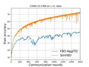
In this section, we perform two hyper-representation experiments to compare the performance of our proposed SimFBO algorithm with FBO-AggITD [69], FedNest [69], and LFedNest [65], and validate the better performance of ShroFBO in the presence of heterogeneous local computation. We test the performance on MNIST and CIFAR datasets with MLP and CNN backbones. We follow the same experimental setup and problem formulation as in [65, 69]. The details of all experimental specifications can be found in Section A.1.

Comparison to existing methods. The comparison results are presented in Figure 2 and Figure 3. It can be seen that across different datasets and backbones, our proposed SimFBO consistently converges much faster than other comparison methods, while achieving a much higher training and test accuracy. We do not plot the curves of FedNest and LFedNest on CIFAR and CNN, because they are hard to converge under various hyperparameter configurations using their source codes.

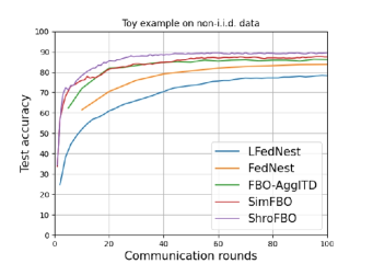
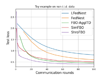
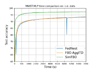
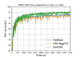
Performance under heterogeneous local computation. We now test the performance in the setting where a total of $10$ clients perform a variable number of local steps. This is to simulate the scenario where clients have heterogeneous computing capabilities and hence can perform an uneven number of local updates. In this experiment, we choose the number $\tau_{i}$ of the client $i$’s local steps from the set $\{1,...,10\}$ uniform at random. As shown in Figure 4, the proposed ShroFBO method performs the best due to the better resilience to such client heterogeneity. We also compare the convergence rate of our proposed SimFBO, FedNest and FBO-AggITD w.r.t. running time. The results are provided in Figure 5. All the settings for different algorithms are the same as in Section A.2. It can be seen that the proposed SimFBO still converges fastest with a higher test accuracy in terms of running time.

Figure 4: Comparison among different algorithms in the presence of heterogeneous local computation.

Figure 5: Time Comparison among different algorithms.

6 Conclusion

In this paper, we propose a simple and communication-efficient federated bilevel algorithm named SimFBO and its variant ShroFBO with better resilience to the system-level heterogeneity. We show that both SimFBO and ShroFBO allow for the more practical client sampling without replacement, and achieve better sample and communication complexities. Experiments demonstrate the great promise of the proposed methods. We anticipate that the proposed algorithms and the developed analysis can be applied to other distributed settings such as decentralized or asynchronous bilevel optimization, and the algorithms may be useful in applications such as hyperparameter tuning or fine-tuning in federated learning or AI-aware edge computing.

Supplementary material

Appendix A Specifications of Experiments

A.1 Model architecture and dataset

MLP. The 2-layer multilayer perceptron (MLP) has 784 input units and 200 hidden units so that the hidden layer parameters (157,000 parameters) are optimized for solving the upper-level problem and the output layer parameters (2,010 parameters) are optimized for solving the lower-level problem.

CNN. We use the 7-layer CNN [33] model to train CIFAR-10. We optimize the last fully connected layer’s parameters for solving the lower-level problem and optimize the rest layers’ parameters for solving the upper-level problem.

Dataset. For the hyper-representation experiment, we use full MNIST and CIFAR-10 datasets. In the experiment with heterogeneous local computation, we treat the first 2000 images in MNIST’s default training dataset as the training data and the first 1000 images in MNIST’s default test dataset as test data.

A.2 Hyperparameter settings

For all comparison methods, we optimize their hyperparameters via grid search guided by the default values in their source codes, to ensure the best performance given the algorithms are convergent.

Comparison to existing methods. First of all, for all methods, 10 clients from 100 clients are chosen randomly and participate in each communication round. For the baseline methods FedNest and LFedNest, we use their published codes in https://github.com/ucr-optml/FedNest. For FBO-AggITD, we use the source codes sent from the authors. For our method, SimFBO, we take the number of local updates,$\tau_{i}$, for each client $i$ to be 1, $a_{i}^{(t,k)}$ to be 1, and $\widetilde{p_{i}}$ to be 0.1. In MNIST-MLP experiment, the stepsizes $[\eta_{y},\eta_{v},\eta_{x}]$ and $[\gamma_{y},\gamma_{v},\gamma_{x}]$ of our method for updating $[y_{i}^{t,k}(y^{t}),v_{i}^{t,k}(v^{t}),x_{i}^{t,k}(x^{t})]$ are both [0.2, 0.1, 0.05], respectively. Second, for the CIFAR-10-CNN experiment under the i.i.d. setup, we only draw the result of FBO-AggITD and SimFBO because other algorithms cannot converge under various hyperparameter configurations. We take the best inner stepsize as 0.003 and the best outer stepsize as 0.005 for FBO-AggITD, and the stepsizes $[\eta_{y},\eta_{v},\eta_{x}]$ and $[\gamma_{y},\gamma_{v},\gamma_{x}]$ of our method for updating $[y_{i}^{t,k}(y^{t}),v_{i}^{t,k}(v^{t}),x_{i}^{t,k}(x^{t})]$ are both [0.1, 0.05, 0.03], respectively.

Performance under heterogeneous local computation. In this experiment, we compare the results among LFedNest, FedNest, FBO-AggITD, SimFBO, and ShroFBO. For all methods, the numbers of local updates of different clients are randomly chosen in the range from 1 to 10 to simulate the system-level heterogeneity and there are a total of 10 clients participating during the entire procedure. In specific, inner stepsizes for LFedNest, FedNest, FBO-AggITD are [0.002, 0.01, 0.005], respectively while outer stepsizes for LFedNest, FedNest, FBO-AggITD are [0.005, 0.03, 0.04], respectively. Other hyperpameters of the above mentioned three methods are chosen the same as in the above experiment. Then for ShroFBO, we keep choosing $a_{i}^{(t,k)}$ for each client $i$ as 1 but the values of $\|a_{j}^{(t)}\|_{1}$ for $j\in[1,n]$ would be different since the number of local updates $\tau_{i}$ is randomly chosen between 1 and 10. The value of $p_{j}$ is chosen as 0.1. Similarly, the stepsizes $[\eta_{y},\eta_{v},\eta_{x}]$ and $[\gamma_{y},\gamma_{v},\gamma_{x}]$ of our method for updating $[y_{i}^{t,k}(y^{t}),v_{i}^{t,k}(v^{t}),x_{i}^{t,k}(x^{t})]$ are both [0.03, 0.02, 0.01], respectively. Lastly, SimFBO has the same settings mentioned above.

Appendix B Notations

For notational convenience, we define

$$\widetilde{F}(x,y):=\sum_{i=1}^{n}w_{i}f_{i}(x,y),\;\widetilde{G}(x,y):=\sum_{i=1}^{n}w_{i}g_{i}(x,y),\;\widetilde{R}(w,y,v):=\sum_{i=1}^{n}w_{i}R_{i}(x,y,v).$$

For SimBFO, the problem we solve here is

$$\min_{x\in\mathbb{R}^{p}}\widetilde{\Phi}(x)=\widetilde{F}(x,\widetilde{y}^{*}(x)):=\sum_{i=1}^{n}w_{i}f_{i}(x,\widetilde{y}^{*}(x))=\sum_{i=1}^{n}w_{i}\mathbb{E}_{\xi}\big{[}f_{i}(x,\widetilde{y}^{*}(x);\xi)\big{]}$$

$$\;\;\mbox{s.t.}\;\widetilde{y}^{*}(x)=\operatorname*{arg\,min}_{y\in\mathbb{R}^{q}}\widetilde{G}(x,y):=\sum_{i=1}^{n}w_{i}g_{i}(x,y)=\sum_{i=1}^{n}w_{i}\mathbb{E}_{\zeta}\big{[}g_{i}(x,y;\zeta)\big{]}.$$

Similarly, we define

$$\widetilde{\Phi}(x):=\widetilde{F}(x,\widetilde{y}^{*}),\;\nabla\widetilde{\Phi}(x):=\sum_{i=1}^{n}w_{i}\bar{\nabla}f(x,\widetilde{y}^{*},\widetilde{v}^{*})$$ (11)

where $\widetilde{y}^{*}=\operatorname*{arg\,min}_{y}\widetilde{G}(x,y)$ and $\widetilde{v}^{*}=\operatorname*{arg\,min}_{v}\widetilde{R}(x,\widetilde{y}^{*},v)$.

We can see that $\widetilde{y}^{*}$ and $\widetilde{v}^{*}$ are unique due to the strong convexity of $g_{i}(x,y)$ and $R_{i}(x,y,v)$. Client updates are aggregated to compute $\{h^{(t)}_{x,i},h^{(t)}_{y,i},h^{(t)}_{v,i}\}$ as

$$h_{y,i}^{(t)} =\frac{1}{\|a_{i}^{(t)}\|_{1}}\sum_{k=1}^{\tau_{i}^{(t)}}a_{i}^{(t,k)}\nabla_{y}g_{i}(x_{i}^{(t,k)},y_{i}^{(t,k)};\zeta_{i}^{(t,k)}),$$

$$h_{v,i}^{(t)} =\frac{1}{\|a_{i}^{(t)}\|_{1}}\sum_{k=1}^{\tau_{i}^{(t)}}a_{i}^{(t,k)}\nabla_{v}R_{i}(x_{i}^{(t,k)},y_{i}^{(t,k)},v_{i}^{(t,k)};\psi_{i}^{(t,k)}),$$

$$h_{x,i}^{(t)} =\frac{1}{\|a_{i}^{(t)}\|_{1}}\sum_{k=1}^{\tau_{i}^{(t)}}a_{i}^{(t,k)}\bar{\nabla}f_{i}(x_{i}^{(t,k)},y_{i}^{(t,k)},v_{i}^{(t,k)};\xi_{i}^{(t,k)}),$$

and their expectations are

$$\widetilde{h}_{y,i}^{(t)} =\mathbb{E}[h_{y,i}^{(t)}]=\frac{1}{\|a_{i}^{(t)}\|_{1}}\sum_{k=1}^{\tau_{i}^{(t)}}a_{i}^{(t,k)}\nabla_{y}g_{i}(x_{i}^{(t,k)},y_{i}^{(t,k)}),$$

$$\widetilde{h}_{v,i}^{(t)} =\mathbb{E}[h_{v,i}^{(t)}]=\frac{1}{\|a_{i}^{(t)}\|_{1}}\sum_{k=1}^{\tau_{i}^{(t)}}a_{i}^{(t,k)}\nabla_{v}R_{i}(x_{i}^{(t,k)},y_{i}^{(t,k)},v_{i}^{(t,k)}),$$

$$\widetilde{h}_{x,i}^{(t)} =\mathbb{E}[h_{x,i}^{(t)}]=\frac{1}{\|a_{i}^{(t)}\|_{1}}\sum_{k=1}^{\tau_{i}^{(t)}}a_{i}^{(t,k)}\bar{\nabla}f_{i}(x_{i}^{(t,k)},y_{i}^{(t,k)},v_{i}^{(t,k)})$$

for all $t\in\{0,1,...,T-1\}$, $k\in\{0,1,...,\tau_{i}-1\}$ and $i\in\{1,2,...,n\}$.

To ensure the robustness of server updates, we set $\alpha_{\min}\leq a_{i}^{(t,k)}\leq\alpha_{\max}$ for all $t=0,1,...,T$, $i=1,2,...n$ and $k=0,1,...,\tau_{i}-1$; we also set $\frac{\beta_{\min}}{n}\leq w_{i}\leq\frac{\beta_{\max}}{n}$ and $\frac{\beta_{\min}^{\prime}}{n}\leq p_{i}\leq\frac{\beta_{\max}^{\prime}}{n}$ for all $i=1,2,...n$.

At global iteration $t$, the server samples $|C^{(t)}|$ clients without replacement (WOR) uniformly at random. On the server side, the aggregated client $i$ update is weighed by $\widetilde{w}_{i}=\frac{n}{|C^{(t)}|}w_{i}$. The aggregates $\{h^{(t)}_{y},h^{(t)}_{v},h^{(t)}_{x}\}$ computed at the server are of the form

$$h^{(t)}_{y}=\sum_{i\in C^{(t)}}\widetilde{w}_{i}h^{(t)}_{y,i},\quad h^{(t)}_{v}=\sum_{i\in C^{(t)}}\widetilde{w}_{i}h^{(t)}_{v,i},\quad h^{(t)}_{x}=\sum_{i\in C^{(t)}}\widetilde{w}_{i}h^{(t)}_{x,i},$$

and we also have partial clients expectation as

$$\mathbb{E}_{C_{(t)}}\big{[}h^{(t)}_{y}\big{]} =\mathbb{E}_{C_{(t)}}\bigg{[}\sum_{i=1}^{n}\mathbb{I}(i\in C^{(t)})\widetilde{w}_{i}h^{(t)}_{y,i}\bigg{]}=\sum_{i=1}^{n}w_{i}h^{(t)}_{y,i},$$

$$\mathbb{E}_{C_{(t)}}\big{[}h^{(t)}_{v}\big{]} =\mathbb{E}_{C_{(t)}}\bigg{[}\sum_{i=1}^{n}\mathbb{I}(i\in C^{(t)})\widetilde{w}_{i}h^{(t)}_{v,i}\bigg{]}=\sum_{i=1}^{n}w_{i}h^{(t)}_{v,i},$$

$$\mathbb{E}_{C_{(t)}}\big{[}h^{(t)}_{x}\big{]} =\mathbb{E}_{C_{(t)}}\bigg{[}\sum_{i=1}^{n}\mathbb{I}(i\in C^{(t)})\widetilde{w}_{i}h^{(t)}_{x,i}\bigg{]}=\sum_{i=1}^{n}w_{i}h^{(t)}_{x,i}.$$

Generally, the expectations we use contain both the expectations of samples and the expectations of clients. And in analysis, we simply define $|C^{(t)}|=P$ for all $t$. And server updates $y^{(t+1)}$, $v^{(t+1)}$, $x^{(t+1)}$ as

$$y^{(t+1)} =y^{(t)}-\rho^{(t)}\gamma_{y}h^{(t)}_{y},$$

$$v^{(t+1)} =\mathcal{P}_{r}\big{(}v^{(t)}-\rho^{(t)}\gamma_{v}h_{v}^{(t)}\big{)},$$

$$x^{(t+1)} =x^{(t)}-\rho^{(t)}\gamma_{x}h_{x}^{(t)},$$

where the auxiliary projection function is defined as $\mathcal{P}_{r}(v):=\min\{1,\frac{r}{\|v\|}\}v$ and $r=\frac{L_{f}}{\mu_{g}}$ is the server side auxiliary projection radius. To simplify the problem, we set $a_{i}^{(t,k)}$ such that $\rho^{(t)}\in[\frac{1}{2}\bar{\rho},\frac{3}{2}\bar{\rho}]$ and $c_{a}^{\prime}\bar{\tau}\alpha_{\min}\leq\|a_{i}^{(t)}\|_{1}\leq c_{a}\bar{\tau}\alpha_{\max}$ for some positive constant $c_{a}$, $c_{a}^{\prime}$ and $i\in C^{(t)}$, where $\bar{\rho}:=\frac{1}{T}\sum_{t=0}^{T-1}\rho^{(t)}$ and $\bar{\tau}:=\sum_{i=1}^{n}\tau_{i}$.

Appendix C Proofs of Preliminary Lemmas

Lemma 1 (Boundedness of $v^{*}$).

Under Assumptions 1 and 2, we have for $v^{*}$ in section 2.2, $\left\lVert v^{*}\right\rVert^{2}\leq\frac{L^{2}_{f}}{\mu^{2}_{g}}.$

Proof.

Remind that we define $v^{*}=\arg\min_{v}R(x,y^{*},v)$, then we have

$$\left\lVert v^{*}\right\rVert^{2}=\left\lVert\big{[}\nabla_{yy}^{2}G(x,y^{*})\big{]}^{-1}\nabla_{y}F(x,y^{*})\right\rVert^{2}\leq\left\lVert\big{[}\nabla_{yy}^{2}G(x,y^{*})\big{]}^{-1}\right\rVert^{2}\left\lVert\nabla_{y}F(x,y^{*})\right\rVert^{2}\overset{(a)}{\leq}r^{2},$$

where (a) follows Assumptions 1, 2 and defines $r:=\frac{L_{f}}{\mu_{g}}$. Then, the proof is complete. ∎

Lemma 2 (Boundedness of local $v$).

Under Assumptions 1 and 2, for each global iteration $t$, client $i$, and local iteration $k=1,2,...,\tau_{i}$, we have

$$r_{i}:=\|v_{i}^{(t,k)}\|\leq\Big{(}1+\frac{\alpha_{\max}}{\alpha_{\min}}\Big{)}r=:r_{\max},$$

where $r=\frac{L_{f}}{\mu_{g}}$ is the server side auxiliary projection radius.

Proof.

By the local update rule of $v_{i}^{(t,k)}$ from step 6 in Algorithm 1, we have

$$v_{i}^{(t,k)} =v_{i}^{(t,k-1)}-\eta_{v}a_{i}^{(t,k-1)}\nabla_{v}R_{i}(x_{i}^{(t,k-1)},y_{i}^{(t,k-1)},v_{i}^{(t,k-1)};\psi_{i}^{(t,k-1)})$$

$$=\big{(}I-\eta_{v}a_{i}^{(t,k-1)}\nabla^{2}_{yy}g_{i}(x_{i}^{(t,k-1)},y_{i}^{(t,k-1)};\psi_{i}^{(t,k-1)})\big{)}v_{i}^{(t,k-1)}$$

$$\quad\ +\eta_{v}a_{i}^{(t,k-1)}\nabla_{y}f_{i}(x_{i}^{(t,k-1)},y_{i}^{(t,k-1)};\psi_{i}^{(t,k-1)}).$$

By taking $l_{2}$ norm, we have

$$\|v_{i}^{(t,k)}\|\leq(1-\eta_{v}a_{i}^{(t,k-1)}\mu_{g})\|v_{i}^{(t,k-1)}\|+\eta_{v}a_{i}^{(t,k-1)}L_{f}.$$ (12)

Telescope eq. 12 over $j\in[0,...,k-1]$, and we have

$$\|v_{i}^{(t,k)}\| \leq(1-\eta_{v}a_{i}^{(t,k-1)}\mu_{g})\|v_{i}^{(t,k-1)}\|+\eta_{v}a_{i}^{(t,k-1)}L_{f}$$

$$\leq(1-\eta_{v}\alpha_{\min}\mu_{g})^{k}\|v_{i}^{(t,0)}\|+\sum_{j=0}^{k-1}(1-\eta\alpha_{\min}\mu_{g})^{j}\eta_{v}\alpha_{\max}L_{f}$$

$$\leq(1-\eta_{v}\alpha_{\min}\mu_{g})^{k}\|v_{i}^{(t,0)}\|+\frac{\alpha_{\max}L_{f}}{\alpha_{\min}\mu_{g}}$$

$$\leq\Big{(}1+\frac{\alpha_{\max}}{\alpha_{\min}}\Big{)}r.$$

Then, the proof is complete. ∎

Since both $\alpha_{\max}$ and $\alpha_{\min}$ are preset constants, the bound of local $v_{i}$ has the same order $\kappa$ as server-side auxiliary projection radius $r$.

Lemma 3 (Basic properties of linear system function R).

Under Assumptions 1 and 2, we have $R_{i}(x,y,v)$ is $\mu_{g}$-strongly convex w.r.t $v$ and $\nabla_{v}R_{i}(x,y,v)$ is $L_{R}$-Lipschitz continuous w.r.t $(x,y)$, where we define $L_{R}^{2}:=2(L^{2}_{2}r^{2}_{\max}+L_{1}^{2})$.

Proof.

The strong convexity can be easily observed since $\nabla_{vv}^{2}R(x,y,v)=\nabla_{yy}^{2}g(x,y)\succeq\mu_{g}I$. By using the definition of $R_{i}(x,y,v)$ and assumptions 1 and 2, we have

$$\|\nabla_{v} R_{i}(x_{1},y_{1},v)-\nabla_{v}R_{i}(x_{2},y_{2},v)\|^{2}$$

$$\leq 2\|\big{(}\nabla_{yy}^{2}g(x_{1},y_{1})-\nabla_{yy}^{2}g(x_{2},y_{2})\big{)}v\|^{2}+2\|\nabla_{y}f(x_{1},y_{1})-\nabla_{y}f(x_{2},y_{2})\|^{2}$$

$$\leq 2(L^{2}_{2}r^{2}_{\max}+L_{1}^{2})(\|x_{1}-x_{2}\|^{2}+\|y_{1}-y_{2}\|^{2})=L_{R}^{2}(\|x_{1}-x_{2}\|^{2}+\|y_{1}-y_{2}\|^{2}).$$

Then, the proof is complete. ∎

Lemma 4 ([15] lemma 2.2, [4] lemma 2 and extensions).

Under Assumptions 1, 2 and  3, we have, for all $x,x_{1},x_{2}\in\mathbb{R}^{d_{x}}$ and $y\in\mathbb{R}^{d_{y}}$,

$$\|\nabla f(x,y)-\nabla\Phi(x)\|^{2}\leq\widetilde{L}^{2}\|y-y^{*}(x)\|^{2}, \ \ \|\nabla\Phi(x_{1})-\nabla\Phi(x_{2})\|^{2}\leq L_{\Phi}^{2}\|x_{1}-x_{2}\|^{2},$$

$$\|y^{*}(x_{1})-y^{*}(x_{2})\|^{2}\leq L_{y}^{2}\|x_{1}-x_{2}\|^{2}, \ \ \|\nabla y^{*}(x_{1})-\nabla y^{*}(x_{2})\|^{2}\leq L_{yx}^{2}\|x_{1}-x_{2}\|^{2},$$

$$\|v^{*}(x_{1})-v^{*}(x_{2})\|^{2}\leq L_{v}^{2}\|x_{1}-x_{2}\|^{2}, \ \ \|\nabla v^{*}(x_{1})-\nabla v^{*}(x_{2})\|^{2}\leq L_{vx}^{2}\|x_{1}-x_{2}\|^{2}$$

where the constants are given by

$$\widetilde{L}=L_{1}+\frac{L_{1}^{2}}{\mu_{g}}+L_{f}\bigg{(}\frac{L_{2}}{\mu_{g}}+ \frac{L_{1}L_{2}}{\mu_{g}^{2}}\bigg{)},\ \ \ L_{\Phi}=\widetilde{L}+\frac{\widetilde{L}L_{1}}{\mu_{g}},$$

$$L_{y}=\frac{L_{1}}{\mu_{g}},\ \ \ L_{v}=\bigg{(}\frac{2L_{1}^{2}}{\mu_{g}^{2}} +\frac{2L_{f}^{2}L_{2}^{2}}{\mu_{g}^{4}}\bigg{)}^{\frac{1}{2}}\big{(}1+L_{y}^{2}\big{)}^{\frac{1}{2}},$$

$$L_{yx}=\frac{L_{2}+L_{2}L_{y}}{\mu_{g}}+\frac{L_{1}(L_{2}+L_{2}L_{y})}{\mu_{g}^{2}},\quad L_{vx}= \frac{2}{\mu_{g}}\Big{(}\big{(}L_{2}^{2}+r^{2}L_{3}^{2}+L_{2}^{2}L_{v}^{2}\big{)}\big{(}1+L_{y}^{2}\big{)}+L_{2}^{2}L_{v}^{2}\Big{)}^{\frac{1}{2}}.$$ (13)

Proof.

The proof of the first 3 inequalities is provided in [15]. For the fifth inequality, we have

$$\big{\|} v^{*}(x_{1})-v^{*}(x_{2})\big{\|}^{2}$$

$$=\Big{\|}\big{[}\nabla^{2}_{yy}G\big{(}x_{1},y^{*}(x_{1})\big{)}\big{]}^{-1}\nabla_{y}F\big{(}x_{1},y^{*}(x_{1})\big{)}-\big{[}\nabla^{2}_{yy}G\big{(}x_{2},y^{*}(x_{2})\big{)}\big{]}^{-1}\nabla_{y}F\big{(}x_{2},y^{*}(x_{2})\big{)}\Big{\|}^{2}$$

$$\leq 2\Big{\|}\big{[}\nabla^{2}_{yy}G\big{(}x_{1},y^{*}(x_{1})\big{)}\big{]}^{-1}\Big{(}\nabla_{y}F\big{(}x_{1},y^{*}(x_{1})\big{)}-\nabla_{y}F\big{(}x_{2},y^{*}(x_{2})\big{)}\Big{)}\Big{\|}^{2}$$

$$\quad+2\Big{\|}\Big{(}\big{[}\nabla^{2}_{yy}G\big{(}x_{1},y^{*}(x_{1})\big{)}\big{]}^{-1}-\big{[}\nabla^{2}_{yy}G\big{(}x_{2},y^{*}(x_{2})\big{)}\big{]}^{-1}\Big{)}\nabla_{y}F\big{(}x_{2},y^{*}(x_{2})\big{)}\Big{\|}^{2}$$

$$\leq\frac{2L_{1}^{2}}{\mu_{g}^{2}}\big{(}\big{\|}x_{1}-x_{2}\big{\|}^{2}+\big{\|}y^{*}(x_{1})-y^{*}(x_{2})\big{\|}^{2}\big{)}$$

$$\quad+2L_{f}^{2}\Big{\|}\big{[}\nabla^{2}_{yy}G\big{(}x_{1},y^{*}(x_{1})\big{)}\big{]}^{-1}\big{[}\nabla^{2}_{yy}G\big{(}x_{1},y^{*}(x_{1})\big{)}-\nabla^{2}_{yy}G\big{(}x_{2},y^{*}(x_{2})\big{)}\big{]}\big{[}\nabla^{2}_{yy}G\big{(}x_{2},y^{*}(x_{2})\big{)}\big{]}^{-1}\Big{\|}^{2}$$

$$\leq\bigg{(}\frac{2L_{1}^{2}}{\mu_{g}^{2}}+\frac{2L_{f}^{2}L_{2}^{2}}{\mu_{g}^{4}}\bigg{)}\big{(}\big{\|}x_{1}-x_{2}\big{\|}^{2}+\big{\|}y^{*}(x_{1})-y^{*}(x_{2})\big{\|}^{2}\big{)}$$

$$\leq\bigg{(}\frac{2L_{1}^{2}}{\mu_{g}^{2}}+\frac{2L_{f}^{2}L_{2}^{2}}{\mu_{g}^{4}}\bigg{)}\big{(}1+L_{y}^{2}\big{)}\big{\|}x_{1}-x_{2}\big{\|}^{2}.$$

And for the sixth inequality, we have

$$\nabla_{v}R\big{(}x,y^{*}(x),v^{*}(x)\big{)}=\nabla_{yy}^{2}G\big{(}x,y^{*}(x)\big{)}v^{*}(x)-\nabla_{y}F\big{(}x,y^{*}(x)\big{)}=0,$$

which implies that

$$\frac{\partial_{x}\nabla_{v}R\big{(}x,y^{*}(x),v^{*}(x)\big{)}}{\partial x} =\big{[}v^{*}(x)\big{]}^{T}\Big{[}\nabla_{yyx}^{3}G\big{(}x,y^{*}(x)\big{)}+\nabla_{yyy}^{3}G\big{(}x,y^{*}(x)\big{)}\nabla y^{*}(x)\Big{]}$$

$$\quad+\nabla_{yy}^{2}G\big{(}x,y^{*}(x)\big{)}\nabla v^{*}(x)-\nabla_{yx}^{2}F\big{(}x,y^{*}(x)\big{)}-\nabla_{yy}^{2}F\big{(}x,y^{*}(x)\big{)}\nabla y^{*}(x)$$

$$=\mathbf{0}_{d^{y},d^{x}}$$ (14)

and

$$\frac{\partial_{y}\nabla_{v}R(x,y^{*}(x),v^{*}(x))}{\partial y}= \big{[}v^{*}(x)\big{]}^{T}\nabla_{yyy}^{3}G\big{(}x,y^{*}(x)\big{)}-\nabla_{yy}^{2}F\big{(}x,y^{*}(x)\big{)}=\mathbf{0}_{d^{y},d^{y}}.$$ (15)

By combining appendix C and eq. 15, we have

$$\nabla_{yy}^{2}G\big{(}x,y^{*}(x)\big{)}\nabla_{x}v^{*}\big{(}x,y^{*}(x)\big{)}= \nabla_{yx}^{2}F\big{(}x,y^{*}(x)\big{)}-\big{[}v^{*}(x)\big{]}^{T}\nabla_{yyx}^{3}G\big{(}x,y^{*}(x)\big{)}.$$ (16)

Then we can get that

$$\nabla_{yy}^{2}G \big{(}x_{1},y^{*}(x_{1})\big{)}\nabla_{x}v^{*}\big{(}x_{1},y^{*}(x_{1})\big{)}-\nabla_{yy}^{2}G\big{(}x_{2},y^{*}(x_{2})\big{)}\nabla_{x}v^{*}\big{(}x_{2},y^{*}(x_{2})\big{)}$$

$$=\nabla_{yy}^{2}G\big{(}x_{1},y^{*}(x_{1})\big{)}\nabla_{x}v^{*}\big{(}x_{1},y^{*}(x_{1})\big{)}-\nabla_{yy}^{2}G\big{(}x_{2},y^{*}(x_{2})\big{)}\nabla_{x}v^{*}\big{(}x_{1},y^{*}(x_{1})\big{)}$$

$$\quad+\nabla_{yy}^{2}G\big{(}x_{2},y^{*}(x_{2})\big{)}\nabla_{x}v^{*}\big{(}x_{1},y^{*}(x_{1})\big{)}-\nabla_{yy}^{2}G\big{(}x_{2},y^{*}(x_{2})\big{)}\nabla_{x}v^{*}\big{(}x_{2},y^{*}(x_{2})\big{)}$$

$$=\Big{[}\nabla_{yx}F\big{(}x_{1},y^{*}(x_{1})\big{)}-\nabla_{yx}F\big{(}x_{2},y^{*}(x_{2})\big{)}\Big{]}$$

$$\quad-\Big{(}\big{[}v^{*}(x_{1})\big{]}^{T}\nabla_{yyx}^{3}G\big{(}x_{1},y^{*}(x_{1})\big{)}-\big{[}v^{*}(x_{2})\big{]}^{T}\nabla_{yyx}^{3}G\big{(}x_{2},y^{*}(x_{2})\big{)}\Big{)}$$

By taking the norm and using Assumption 2, we have

$$\bigg{\|}\nabla_{yy}^{2} G\big{(}x_{2},y^{*}(x_{2})\big{)}\Big{[}\nabla_{x}v^{*}(x_{1})-\nabla_{x}v^{*}(x_{2})\big{)}\Big{]}\bigg{\|}^{2}$$

$$\leq 4\bigg{\|}\nabla_{xy}^{2}F\big{(}x_{1},y^{*}(x_{1})\big{)}-\nabla_{xy}^{2}F\big{(}x_{2},y^{*}(x_{2})\big{)}\bigg{\|}^{2}$$

$$\quad+4\bigg{\|}\big{[}v^{*}(x_{1})-v^{*}(x_{2})\big{]}^{T}\nabla_{yyx}^{3}G\big{(}x_{2},y^{*}(x_{2})\big{)}\bigg{\|}^{2}$$

$$\quad+4\bigg{\|}\big{[}v^{*}(x_{1})\big{]}^{T}\Big{[}\nabla_{yyx}^{3}G\big{(}x_{1},y^{*}(x_{1})\big{)}-\nabla_{yyx}^{3}G\big{(}x_{2},y^{*}(x_{2})\big{)}\Big{]}\bigg{\|}^{2}$$

$$\quad+4\bigg{\|}\Big{[}\nabla_{yy}^{2}G\big{(}x_{1},y^{*}(x_{1})\big{)}-\nabla_{yy}^{2}G\big{(}x_{2},y^{*}(x_{2})\big{)}\Big{]}\nabla_{x}v^{*}(x_{1})\bigg{\|}^{2}$$

$$\leq 4\Big{(}L_{2}^{2}+r^{2}L_{3}^{2}+L_{2}^{2}L_{v}^{2}\Big{)}\Big{(}\big{\|}x_{1}-x_{2}\big{\|}^{2}+\big{\|}y^{*}(x_{1})-y^{*}(x_{2})\big{\|}^{2}\Big{)}+4\Big{(}L_{2}^{2}L_{v}^{2}\Big{)}\big{\|}x_{1}-x_{2}\big{\|}^{2}$$

$$\leq 4\Big{(}\big{(}L_{2}^{2}+r^{2}L_{3}^{2}+L_{2}^{2}L_{v}^{2}\big{)}\big{(}1+L_{y}^{2}\big{)}+L_{2}^{2}L_{v}^{2}\Big{)}\big{\|}x_{1}-x_{2}\big{\|}^{2}$$ (17)

By using the strong convexity of $g_{i}$ in Assumption 1, we have

$$\Big{\|}\nabla_{x}v^{*}\big{(}x_{1},y^{*}(x_{1})\big{)}-\nabla_{x}v^{*}\big{(}x_{2},y^{*}(x_{2})\big{)}\Big{\|}^{2}\leq L_{vx}^{2}\big{\|}x_{1}-x_{2}\big{\|}^{2},$$ (18)

where $L_{vx}=\frac{2}{\mu_{g}}\Big{(}\big{(}L_{2}^{2}+r^{2}L_{3}^{2}+L_{2}^{2}L_{v}^{2}\big{)}\big{(}1+L_{y}^{2}\big{)}+L_{2}^{2}L_{v}^{2}\Big{)}^{\frac{1}{2}}$. Then the proof is complete. ∎

Lemma 5 (Global Heterogeneity Extension).

For any set of non-negative weight $\{w_{i}\}_{i=1}^{n}$ such that $\sum_{i=1}^{n}w_{i}=1$, under Assumption 2 and Lemma 2, we have the bounds of global heterogeneity of $\nabla g_{i}(x,y)$, $\nabla R_{i}(x,y,v)$ and $\nabla f_{i}(x,y,v)$ as

$$\sum_{i=1}^{n}w_{i}\|\nabla_{y}g_{i}(x,y)\|^{2}\leq\beta_{gh}^{2} L_{1}^{2}\big{\|}y-y^{*}(x)\big{\|}^{2}+\sigma_{gh}^{2},$$

$$\sum_{i=1}^{n}w_{i}\|\nabla_{v}R_{i}(x,y,v)\|^{2} \leq 2r_{\max}^{2}L_{1}^{2}+2L_{f}^{2},$$

$$\sum_{i=1}^{n}w_{i}\|\bar{\nabla}f_{i}(x,y,v)\|^{2} \leq 2r_{\max}^{2}L_{1}^{2}+2L_{f}^{2}$$

for all $i\in\{1,...,n\}$.

Proof.

Under Assumption 4, we have

$$\sum_{i=1}^{n}w_{i}\|\nabla_{y}g_{i}(x,y)\|^{2} \leq\beta_{gh}^{2}\bigg{\|}\sum_{i=1}^{n}w_{i}\Big{[}\nabla_{y}g_{i}(x,y)-\nabla_{y}g_{i}\big{(}x,y^{*}(x)\big{)}\Big{]}\bigg{\|}^{2}+\sigma_{gh}^{2}$$

$$\leq\beta_{gh}^{2}L_{1}^{2}\big{\|}y-y^{*}(x)\big{\|}^{2}+\sigma_{gh}^{2}.$$

For $R_{i}$ and $f_{i}$, we can easily have

$$\|\nabla_{v}R_{i}(x,y,v)\|^{2} \leq 2\|\nabla_{yy}g(x,y)v\|^{2}+2\|\nabla_{y}f(x,y)\|^{2}\leq 2r_{\max}^{2}L_{1}^{2}+2L_{f}^{2},$$

$$\|\bar{\nabla}f_{i}(x,y,v)\|^{2} \leq 2\|\nabla_{xy}g(x,y)v\|^{2}+2\|\nabla_{x}f(x,y)\|^{2}\leq 2r_{\max}^{2}L_{1}^{2}+2L_{f}^{2}.$$

Then the proof is complete. ∎

Lemma 6.

Under Assumption 2, we have the following bounds

$$\big{\|}\bar{\nabla}f_{i}(x^{(t)},y^{(t)},v^{(t)}) -\bar{\nabla}f_{i}(x_{i}^{(t,k)},y_{i}^{(t,k)},v_{i}^{(t,k)})\big{\|}^{2}\leq\Delta_{f,i}^{(t,k)},$$

$$\big{\|}\nabla g_{i}(x^{(t)},y^{(t)}) -\nabla g_{i}(x_{i}^{(t,k)},y_{i}^{(t,k)})\big{\|}^{2}\leq\Delta_{g,i}^{(t,k)},$$

$$\big{\|}\nabla_{v}R_{i}(x^{(t)},y^{(t)},v^{(t)}) -\nabla R_{i}(x_{i}^{(t,k)},y_{i}^{(t,k)},v_{i}^{(t,k)})\big{\|}^{2}\leq\Delta_{R,i}^{(t,k)},$$

where we define the combinations of client drift from as

$$\Delta_{f_{i}}^{(t,k)}=\Delta_{R_{i}}^{(t,k)}:=3\big{(}L^{2}_{1} +r^{2}L^{2}_{2}\big{)}\Big{[}\big{\|}x_{i}^{(t,k)}-x^{(t)}\big{\|}^{2}+\big{\|}y_{i}^{(t,k)}-y^{(t)}\big{\|}^{2}\Big{]}+3L^{2}_{1}\big{\|}v_{i}^{(t,k)}-v^{(t)}\big{\|}^{2}$$

$$\Delta_{g_{i}}^{(t,k)} :=L_{1}^{2}\Big{[}\big{\|}x_{i}^{(t,k)}-x^{(t)}\big{\|}^{2}+\big{\|}y_{i}^{(t,k)}-y^{(t)}\big{\|}^{2}\Big{]}.$$

Proof.

According to the definition, we have

$$\big{\|}\bar{\nabla}f_{i}(x^{(t)}, y^{(t)},v^{(t)})-\bar{\nabla}f_{i}(x_{i}^{(t,k)},y_{i}^{(t,k)},v_{i}^{(t,k)})\big{\|}^{2}$$

$$\leq\big{\|}\nabla_{x}f_{i}(x^{(t)},y^{(t)},v^{(t)})-\nabla_{x}f_{i}(x_{i}^{(t,k)},y_{i}^{(t,k)},v_{i}^{(t,k)})$$

$$\quad-\nabla_{xy}^{2}g_{i}(x^{(t)},y^{(t)},v^{(t)})v^{(t)}+\nabla_{xy}^{2}g_{i}(x_{i}^{(t,k)},y_{i}^{(t,k)},v_{i}^{(t,k)})v_{i}^{(t,k)}\big{\|}^{2}$$

$$\leq 3\big{\|}\nabla_{x}f_{i}(x^{(t)},y^{(t)},v^{(t)})-\nabla_{x}f_{i}(x_{i}^{(t,k)},y_{i}^{(t,k)},v_{i}^{(t,k)})\big{\|}^{2}$$

$$\quad+3\big{\|}\big{(}\nabla_{xy}^{2}g_{i}(x^{(t)},y^{(t)},v^{(t)})-\nabla_{xy}^{2}g_{i}(x_{i}^{(t,k)},y_{i}^{(t,k)},v_{i}^{(t,k)})\big{)}v^{(t)}\big{\|}^{2}$$

$$\quad+3\big{\|}\nabla_{xy}^{2}g_{i}(x_{i}^{(t,k)},y_{i}^{(t,k)},v_{i}^{(t,k)})\big{(}v^{(t)}-v_{i}^{(t,k)}\big{)}\big{\|}^{2}$$

$$\overset{(a)}{\leq}3\big{(}L^{2}_{1}+r^{2}L^{2}_{2}\big{)}\Big{[}\big{\|}x_{i}^{(t,k)}-x^{(t)}\big{\|}^{2}+\big{\|}y_{i}^{(t,k)}-y^{(t)}\big{\|}^{2}\Big{]}+3L^{2}_{1}\big{\|}v_{i}^{(t,k)}-v^{(t)}\big{\|}^{2},$$

where (a) follows from Assumption2 and Lemma 1. Similarly, we can easily get the results of $\nabla g_{i}$ and $\nabla_{v}R_{i}$, then the proof is complete. ∎

Appendix D Proofs of Theorem 1

D.1 Descent in Objective Function

Lemma 7.

Under Asusmption 1, for non-convex and smooth $\widetilde{\Phi}(x)$, the consecutive iterates of Algorithm 1 satisfy:

$$\mathbb{E}[\widetilde{\Phi}(x^{(t+1)})] -\mathbb{E}[\widetilde{\Phi}(x^{(t)})]$$

$$\leq -\frac{\rho^{(t)}\gamma_{x}}{2}\Big{(}\mathbb{E}\|\nabla\widetilde{\Phi}(x^{(t)})\|^{2}+\mathbb{E}\Big{\|}\sum_{i=1}^{n}w_{i}\widetilde{h}^{(t)}_{x,i}\Big{\|}^{2}\Big{)}$$

$$+\frac{\rho^{(t)}\gamma_{x}}{2}\Big{(}6(L^{2}_{1}+r^{2}L^{2}_{2})\mathbb{E}\|y^{(t)}-\widetilde{y}^{*}(x^{(t)})\|^{2}+3L^{2}_{1}\mathbb{E}\|v^{(x^{(t)})}-\widetilde{v}^{*}(x^{(t)})\|^{2}\Big{)}$$

$$+\frac{3\rho^{(t)}\gamma_{x}}{2}\sum_{i=1}^{n}w_{i}\frac{1}{\|a_{i}^{(t)}\|_{1}}\sum_{k=0}^{\tau_{i}-1}a^{(t,k)}_{i}\Delta^{(t,k)}_{f,i}+\frac{L_{\Phi}^{2}(\rho^{(t)}\gamma_{x})^{2}}{2}\Big{\|}\sum_{i\in C^{(t)}}\widetilde{w}_{i}h^{(t)}_{x,i}\Big{\|}^{2}$$

for all $t\in\{0,1,...,T-1\}$.

Proof.

Using the $L_{\Phi}$ in Lemma 4, we have

$$\mathbb{E}\big{[}\widetilde{\Phi}(x^{(t+1)} )\big{]}\leq\mathbb{E}\big{[}\widetilde{\Phi}(x^{(t)})\big{]}-\mathbb{E}\Big{\langle}\nabla\widetilde{\Phi}(x^{(t)}),\rho^{(t)}\gamma_{x}\sum_{i\in C^{(t)}}\widetilde{w}_{i}h_{x,i}^{(t,k)}\Big{\rangle}$$

$$\quad\quad+\frac{\big{(}\rho^{(t)}\gamma_{x}\big{)}^{2}L_{\Phi}^{2}}{2}\mathbb{E}\bigg{\|}\sum_{i\in C^{(t)}}\widetilde{w}_{i}h_{x,i}^{(t,k)}\bigg{\|}^{2}$$

$$\overset{(a)}{=}\mathbb{E}\big{[}\widetilde{\Phi}(x^{(t)})\big{]}-\rho^{(t)}\gamma_{x}\mathbb{E}\Big{\langle}\nabla\widetilde{\Phi}(x^{(t)}),\sum_{i=1}^{n}w_{i}\widetilde{h}_{x,i}^{(t,k)}\Big{\rangle}$$

$$\quad+\frac{\big{(}\rho^{(t)}\gamma_{x}\big{)}^{2}L_{\Phi}^{2}}{2}\mathbb{E}\bigg{\|}\sum_{i\in C^{(t)}}\widetilde{w}_{i}h_{x,i}^{(t,k)}\bigg{\|}^{2}$$

$$=\mathbb{E}\big{[}\widetilde{\Phi}(x^{(t)})\big{]}-\frac{\rho^{(t)}\gamma_{x}}{2}\mathbb{E}\Bigg{[}\bigg{\|}\nabla\widetilde{\Phi}(x^{(t)})\bigg{\|}^{2}+\bigg{\|}\sum_{i=1}^{n}w_{i}\widetilde{h}_{x,i}^{(t,k)}\bigg{\|}^{2}\Bigg{]}$$

$$\quad+\frac{\rho^{(t)}\gamma_{x}}{2}\mathbb{E}\bigg{\|}\nabla\widetilde{\Phi}(x^{(t)})-\sum_{i=1}^{n}w_{i}\widetilde{h}_{x,i}^{(t,k)}\bigg{\|}^{2}+\frac{\big{(}\rho^{(t)}\gamma_{x}\big{)}^{2}L_{\Phi}^{2}}{2}\mathbb{E}\bigg{\|}\sum_{i\in C^{(t)}}\widetilde{w}_{i}h_{x,i}^{(t,k)}\bigg{\|}^{2},$$ (19)

where (a) holds because clients are selected without replacement. For the third part of the right-hand side in section D.1, we have

$$\mathbb{E}\bigg{\|} \nabla\widetilde{\Phi}(x^{(t)})-\sum_{i=1}^{n}w_{i}\widetilde{h}_{x,i}^{(t,k)}\bigg{\|}^{2}$$

$$=\mathbb{E}\bigg{\|}\sum_{i=1}^{n}w_{i}\Big{[}\bar{\nabla}f_{i}\big{(}x^{(t)},y^{*}(x^{(t)}),v^{*}(x^{(t)})\big{)}-\bar{\nabla}f_{i}\big{(}x^{(t)},y^{(t)},v^{*}(x^{(t)})\big{)}+\bar{\nabla}f_{i}\big{(}x^{(t)},y^{(t)},v^{*}(x^{(t)})\big{)}$$

$$\qquad\qquad\qquad-\bar{\nabla}f_{i}\big{(}x^{(t)},y^{(t)},v^{(t)}\big{)}+\bar{\nabla}f_{i}(x^{(t)},y^{(t)},v^{(t)})-\widetilde{h}_{x,i}^{(t)}\Big{]}\bigg{\|}^{2}$$

$$\leq 3\mathbb{E}\bigg{\|}\sum_{i=1}^{n}w_{i}\Big{[}\big{(}\nabla_{x}f_{i}(x^{(t)},y^{*}(x^{(t)}))-\nabla_{x}f_{i}(x^{(t)},y^{(t)})\big{)}$$

$$\qquad\qquad\qquad-\big{(}\nabla^{2}_{xy}g_{i}(x^{(t)},y^{*}(x^{(t)}))-\nabla^{2}_{xy}g_{i}(x^{(t)},y^{(t)})\big{)}v^{*}(x)\big{)}\Big{]}\bigg{\|}^{2}$$

$$\quad+3\mathbb{E}\Big{\|}\sum_{i=1}^{n}w_{i}\nabla^{2}_{xy}g_{i}(x^{(t)},y^{(t)})\big{(}v^{*}(x^{(t)})-v^{(t)}\big{)}\Big{\|}^{2}$$

$$\quad+3\mathbb{E}\Big{\|}\sum_{i=1}^{n}w_{i}\big{(}\bar{\nabla}f_{i}(x^{(t)},y^{(t)},v^{(t)})-\widetilde{h}_{x,i}^{(t)}\big{)}\Big{\|}^{2}$$

$$\overset{(a)}{\leq}6\big{(}L^{2}_{1}+r^{2}L_{2}^{2}\big{)}\mathbb{E}\big{\|}y^{*}{(x^{(t)})}-y^{(t)}\big{\|}^{2}+3L^{2}_{1}\mathbb{E}\big{\|}v^{*}{(x^{(t)})}-v^{(t)}\big{\|}^{2}$$

$$\quad+3\sum_{i=1}^{n}w_{i}\sum_{k=0}^{\tau_{i}-1}\frac{a_{i}^{(t,k)}}{\|a_{i}^{(t)}\|_{1}}\mathbb{E}\big{\|}\bar{\nabla}f_{i}(x^{(t)},y^{(t)},v^{(t)})-\bar{\nabla}f_{i}(x_{i}^{(t,k)},y_{i}^{(t,k)},v_{i}^{(t,k)})\big{\|}^{2}$$

$$\overset{(b)}{\leq}6\big{(}L^{2}_{1}+r^{2}L_{2}^{2}\big{)}\mathbb{E}\big{\|}y^{*}{(x^{(t)})}-y^{(t)}\big{\|}^{2}+3L^{2}_{1}\mathbb{E}\big{\|}v^{*}{(x^{(t)})}-v^{(t)}\big{\|}^{2}+3\sum_{i=1}^{n}w_{i}\sum_{k=0}^{\tau_{i}-1}\frac{a_{i}^{(t,k)}}{\|a_{i}^{(t)}\|_{1}}\Delta_{f,i}^{(t,k)},$$

where (a) follows from smoothness of $\nabla_{x}f_{i}(x,y)$ and $L_{2}$-Lipschitz continuity of $\nabla^{2}_{g_{xy}}g(x,y)$ in Assumption 2 and (b) uses Lemma 6. ∎

D.2 Bounds of Client Drifts

Lemma 8.

Under Assumption 1, 2 and 4, the local iterates client drifts of $y_{i}^{(t,k)},v_{i}^{(t,k)},x_{i}^{(t,k)}$ are bounded as

$$\sum_{i=1}^{n}w_{i}\frac{1}{\|a_{i}^{(t)}\|_{1}}\sum_{k=1}^{\tau_{i}-1}a^{(t,k)}_{i}\mathbb{E}\|x^{(t,k)}_{i}-x^{(t)}\|^{2} \leq\eta^{2}_{x}\bar{\tau}\sigma_{M1}^{2},$$

$$\sum_{i=1}^{n}w_{i}\frac{1}{\|a_{i}^{(t)}\|_{1}}\sum_{k=1}^{\tau_{i}-1}a^{(t,k)}_{i}\mathbb{E}\|v^{(t,k)}_{i}-v^{(t)}\|^{2} \leq\eta^{2}_{v}\bar{\tau}\sigma_{M1}^{2},$$

$$\sum_{i=1}^{n}w_{i}\frac{1}{\|a_{i}^{(t)}\|_{1}}\sum_{k=1}^{\tau_{i}-1}a^{(t,k)}_{i}\mathbb{E}\|y^{(t,k)}_{i}-y^{(t)}\|^{2} \leq\frac{\eta_{y}^{2}\bar{\tau}}{1-2\eta_{y}^{2}c_{a}\bar{\tau}\alpha_{\max}L_{1}^{2}}\bigg{[}\alpha_{\max}^{2}\sigma^{2}_{g}+2c_{a}\alpha_{\max}L_{1}^{2}\eta^{2}_{x}\bar{\tau}\sigma_{M1}^{2}$$

$$\qquad+2c_{a}\alpha_{\max}L_{1}^{2}\mathbb{E}\big{\|}y^{(t)}-y^{*}{(x^{(t)})}\big{\|}^{2}+2c_{a}\alpha_{\max}\sigma_{gh}^{2}\bigg{]}$$

for all $t\in\{0,1,...,T-1\}$, $k\in\{0,1,...,\tau_{i}-1\}$ and $i\in\{1,2,...,n\}$. We define $\sigma_{M1}^{2}:=\Big{(}\alpha_{\max}^{2}(\sigma^{2}_{f}+r_{\max}^{2}\sigma^{2}_{gg})+\alpha_{\max}(L_{f}^{2}+r^{2}_{\max}L^{2}_{1})\Big{)}$. And $\eta_{y}$, $\eta_{v}$, $\eta_{x}$ are local stepsizes.

Proof.

For $\big{\|}y^{(t,k)}_{i}-y^{(t)}\big{\|}^{2}$, we have

$$\sum_{i=1}^{n}w_{i}\sum_{k=0}^{\tau_{i}-1}\frac{a_{i}^{(t,k)}}{\|a_{i}^{(t)}\|_{1}}\mathbb{E}\big{\|}y^{(t,k)}_{i}-y^{(t)}\big{\|}^{2}$$

$$=\eta_{y}^{2}\sum_{i=1}^{n}w_{i}\sum_{k=0}^{\tau_{i}-1}\frac{a_{i}^{(t,k)}}{\|a_{i}^{(t)}\|_{1}}\mathbb{E}\bigg{\|}\sum_{j=0}^{k-1}a_{i}^{(t,j)}\Big{(}\nabla_{y}g_{i}\big{(}x_{i}^{(t,j)},y_{i}^{(t,j)};\zeta_{i}^{(t,j)}\big{)}$$

$$\qquad\qquad\qquad\qquad\qquad\qquad\qquad\qquad-\nabla_{y}g_{i}\big{(}x_{i}^{(t,j)},y_{i}^{(t,j)}\big{)}+\nabla_{y}g_{i}\big{(}x_{i}^{(t,j)},y_{i}^{(t,j)}\big{)}\Big{)}\bigg{\|}^{2}$$

$$=\eta_{y}^{2}\sum_{i=1}^{n}w_{i}\sum_{k=0}^{\tau_{i}-1}\frac{a_{i}^{(t,k)}}{\|a_{i}^{(t)}\|_{1}}\sum_{j=0}^{k-1}\Big{(}a_{i}^{(t,j)}\Big{)}^{2}\mathbb{E}\Big{\|}\nabla_{y}g_{i}\big{(}x_{i}^{(t,j)},y_{i}^{(t,j)};\zeta_{i}^{(t,j)}\big{)}-\nabla_{y}g_{i}\big{(}x_{i}^{(t,j)},y_{i}^{(t,j)}\big{)}\Big{\|}^{2}$$

$$\quad+\eta_{y}^{2}\sum_{i=1}^{n}w_{i}\sum_{k=0}^{\tau_{i}-1}\frac{a_{i}^{(t,k)}}{\|a_{i}^{(t)}\|_{1}}\mathbb{E}\Big{\|}\sum_{j=0}^{k-1}a_{i}^{(t,j)}\nabla_{y}g_{i}\big{(}x_{i}^{(t,j)},y_{i}^{(t,j)}\big{)}\Big{\|}^{2}$$

$$\leq\eta_{y}^{2}\sum_{i=1}^{n}w_{i}\sum_{k=0}^{\tau_{i}-1}\frac{a_{i}^{(t,k)}}{\|a_{i}^{(t)}\|_{1}}\sum_{j=0}^{k-1}\Big{(}a_{i}^{(t,j)}\Big{)}^{2}\sigma^{2}_{g}$$

$$\quad+2\eta_{y}^{2}\sum_{i=1}^{n}w_{i}\sum_{k=0}^{\tau_{i}-1}\frac{a_{i}^{(t,k)}}{\|a_{i}^{(t)}\|_{1}}\sum_{j=0}^{k-1}a_{i}^{(t,j)}\mathbb{E}\Big{\|}\nabla_{y}g_{i}\big{(}x_{i}^{(t,j)},y_{i}^{(t,j)}\big{)}-\nabla_{y}g_{i}\big{(}x^{(t)},y^{(t)}\big{)}\Big{\|}^{2}$$

$$\quad+2\eta_{y}^{2}\sum_{i=1}^{n}w_{i}\sum_{k=0}^{\tau_{i}-1}\frac{a_{i}^{(t,k)}}{\|a_{i}^{(t)}\|_{1}}\sum_{j=0}^{k-1}a_{i}^{(t,j)}\mathbb{E}\Big{\|}\nabla_{y}g_{i}\big{(}x^{(t)},y^{(t)}\big{)}\Big{\|}^{2}$$

$$\overset{(a)}{\leq}\eta_{y}^{2}\sum_{i=1}^{n}w_{i}\big{\|}a_{i}^{(t)}\big{\|}_{2}^{2}\sigma^{2}_{g}+2\eta_{y}^{2}\sum_{i=1}^{n}w_{i}\sum_{k=0}^{\tau_{i}-1}\frac{a_{i}^{(t,k)}}{\|a_{i}^{(t)}\|_{1}}\mathbb{E}\Big{\|}\nabla_{y}g_{i}\big{(}x_{i}^{(t,j)},y_{i}^{(t,j)}\big{)}-\nabla_{y}g_{i}\big{(}x^{(t)},y^{(t)}\big{)}\Big{\|}^{2}$$

$$\quad+2\eta_{y}^{2}\sum_{i=1}^{n}w_{i}\big{\|}a_{i}^{(t)}\big{\|}_{1}\mathbb{E}\Big{\|}\nabla_{y}g_{i}\big{(}x^{(t)},y^{(t)}\big{)}\Big{\|}^{2}$$

$$\overset{(b)}{\leq}\eta_{y}^{2}\bar{\tau}\alpha_{\max}^{2}\sigma^{2}_{g}+2\eta_{y}^{2}c_{a}\bar{\tau}\alpha_{\max}\sum_{i=1}^{n}w_{i}\sum_{k=0}^{\tau_{i}-1}\frac{a_{i}^{(t,k)}}{\|a_{i}^{(t)}\|_{1}}\mathbb{E}\Big{\|}\nabla_{y}g_{i}\big{(}x_{i}^{(t,j)},y_{i}^{(t,j)}\big{)}-\nabla_{y}g_{i}\big{(}x^{(t)},y^{(t)}\big{)}\Big{\|}^{2}$$

$$\quad+2\eta_{y}^{2}c_{a}\bar{\tau}\alpha_{\max}\mathbb{E}\bigg{\|}\sum_{i=1}^{n}w_{i}\Big{[}\nabla_{y}g_{i}\big{(}x^{(t)},y^{(t)}\big{)}-\nabla_{y}g_{i}\big{(}x^{(t)},y^{*}{(x^{(t)})}\big{)}\Big{]}\bigg{\|}^{2}+2\eta_{y}^{2}c_{a}\bar{\tau}\alpha_{\max}\sigma_{gh}^{2}$$

$$\overset{(c)}{\leq}\eta_{y}^{2}\bar{\tau}\alpha_{\max}^{2}\sigma^{2}_{g}+2\eta_{y}^{2}c_{a}\bar{\tau}\alpha_{\max}\sum_{i=1}^{n}w_{i}\sum_{k=0}^{\tau_{i}-1}\frac{a_{i}^{(t,k)}}{\|a_{i}^{(t)}\|_{1}}L_{1}^{2}\mathbb{E}\Big{[}\big{\|}x_{i}^{(t,j)}-x^{(t)}\big{\|}^{2}+\big{\|}y_{i}^{(t,j)}-y^{(t)}\big{\|}^{2}\Big{]}$$

$$\quad+2\eta_{y}^{2}c_{a}\bar{\tau}\alpha_{\max}L_{1}^{2}\mathbb{E}\big{\|}y^{(t)}-y^{*}{(x^{(t)})}\big{\|}^{2}+2\eta_{y}^{2}c_{a}\bar{\tau}\alpha_{\max}\sigma_{gh}^{2}$$ (20)

where (a) holds because of Assumption3 and

$$\frac{1}{\|a_{i}^{(t)}\|_{1}}\sum_{k=0}^{\tau_{i}-1}a_{i}^{(t,k)}\sum_{j=0}^{k-1}\Big{(}a_{i}^{(t,j)}\Big{)}^{2} \leq\frac{1}{\|a_{i}^{(t)}\|_{1}}\sum_{k=0}^{\tau_{i}-1}a_{i}^{(t,k)}\sum_{j=0}^{\tau_{i}-2}\Big{(}a_{i}^{(t,j)}\Big{)}^{2}=\sum_{j=0}^{\tau_{i}-2}\Big{(}a_{i}^{(t,j)}\Big{)}^{2}\leq\|a_{i}\|_{2}^{2}$$

$$\frac{1}{\|a_{i}^{(t)}\|_{1}}\sum_{k=0}^{\tau_{i}-1}a_{i}^{(t,k)}\sum_{j=0}^{k-1}a_{i}^{(t,j)} \leq\frac{1}{\|a_{i}^{(t)}\|_{1}}\sum_{k=0}^{\tau_{i}-1}a_{i}^{(t,k)}\sum_{j=0}^{\tau_{i}-2}a_{i}^{(t,j)}=\sum_{j=0}^{\tau_{i}-2}a_{i}^{(t,j)}\leq\|a_{i}^{(t)}\|_{1};$$

(b) is obtained from Assumption4 and (c) follows from Assumption2. As an easier case, we can easily know that $\bar{\nabla}f_{i}$ and $\nabla_{v}R_{i}$ are bounded from Assumption 2 and Lemma 2. Then we have

$$\sum_{i=1}^{n}w_{i} \frac{1}{\|a_{i}^{(t)}\|_{1}}\sum_{k=1}^{\tau_{i}-1}a^{(t,k)}_{i}\mathbb{E}\|x^{(t,k)}_{i}-x^{(t)}\|^{2}\leq\eta^{2}_{x}\bar{\tau}\Big{(}\alpha_{\max}^{2}(\sigma^{2}_{f}+r_{\max}^{2}\sigma^{2}_{gg})+\alpha_{\max}(L_{f}^{2}+r^{2}_{\max}L^{2}_{1})\Big{)},$$

$$\sum_{i=1}^{n}w_{i} \frac{1}{\|a_{i}^{(t)}\|_{1}}\sum_{k=1}^{\tau_{i}-1}a^{(t,k)}_{i}\mathbb{E}\|v^{(t,k)}_{i}-v^{(t)}\|^{2}\leq\eta^{2}_{v}\bar{\tau}\Big{(}\alpha_{\max}^{2}(\sigma^{2}_{f}+r_{\max}^{2}\sigma^{2}_{gg})+\alpha_{\max}(L_{f}^{2}+r^{2}_{\max}L^{2}_{1})\Big{)},$$

$$\sum_{i=1}^{n}w_{i} \frac{1}{\|a_{i}^{(t)}\|_{1}}\sum_{k=1}^{\tau_{i}-1}a^{(t,k)}_{i}\mathbb{E}\|y^{(t,k)}_{i}-y^{(t)}\|^{2}$$

$$\leq\frac{\eta_{y}^{2}\bar{\tau}}{1-2\eta_{y}^{2}c_{a}\bar{\tau}\alpha_{\max}L_{1}^{2}}\bigg{[}\alpha_{\max}^{2}\sigma^{2}_{g}+2c_{a}\alpha_{\max}L_{1}^{2}\eta^{2}_{x}\bar{\tau}\Big{(}\alpha_{\max}^{2}(\sigma^{2}_{f}+r_{\max}^{2}\sigma^{2}_{gg})+\alpha_{\max}(L_{f}^{2}+r^{2}_{\max}L^{2}_{1})\Big{)}$$

$$\qquad\qquad\qquad\qquad\qquad+2c_{a}\alpha_{\max}L_{1}^{2}\mathbb{E}\big{\|}y^{(t)}-y^{*}{(x^{(t)})}\big{\|}^{2}+2c_{a}\alpha_{\max}\sigma_{gh}^{2}\bigg{]}$$

which finished the proof. ∎

In the later part, we will take $\{2\eta_{x}^{2}\bar{\tau}c_{a}\alpha_{\max}L_{1}^{2}\leq 1\}$ and $\{4\eta_{y}^{2}c_{a}\bar{\tau}\alpha_{\max}L_{1}^{2}\leq 1\}$, then we can simplify Lemma 8 as

$$\sum_{i=1}^{n}w_{i} \frac{1}{\|a_{i}^{(t)}\|_{1}}\sum_{k=1}^{\tau_{i}-1}a^{(t,k)}_{i}\mathbb{E}\|x^{(t,k)}_{i}-x^{(t)}\|^{2}\leq\eta^{2}_{x}\bar{\tau}\sigma_{M1}^{2},$$

$$\sum_{i=1}^{n}w_{i} \frac{1}{\|a_{i}^{(t)}\|_{1}}\sum_{k=1}^{\tau_{i}-1}a^{(t,k)}_{i}\mathbb{E}\|v^{(t,k)}_{i}-v^{(t)}\|^{2}\leq\eta^{2}_{v}\bar{\tau}\sigma_{M1}^{2},$$

$$\sum_{i=1}^{n}w_{i} \frac{1}{\|a_{i}^{(t)}\|_{1}}\sum_{k=1}^{\tau_{i}-1}a^{(t,k)}_{i}\mathbb{E}\|y^{(t,k)}_{i}-y^{(t)}\|^{2}\leq 2\eta_{y}^{2}\bar{\tau}\sigma_{M2}^{2}+4\eta_{y}^{2}\bar{\tau}c_{a}\alpha_{\max}L_{1}^{2}\mathbb{E}\big{\|}y^{(t)}-y^{*}{(x^{(t)})}\big{\|}^{2}$$ (21)

where we define $\sigma_{M2}^{2}:=\alpha_{\max}^{2}\sigma^{2}_{g}+\alpha_{\max}^{2}(\sigma^{2}_{f}+r_{\max}^{2}\sigma^{2}_{gg})+\alpha_{\max}(L_{f}^{2}+r^{2}_{\max}L^{2}_{1})+2c_{a}\alpha_{\max}\sigma_{gh}^{2}$. As the combination of Lemma 6 and Lemma 8, we have

$$\sum_{i=1}^{n}w_{i}\sum_{k=1}^{\tau_{i}-1}\frac{a^{(t,k)}_{i}}{\|a_{i}^{(t)}\|_{1}}\Delta_{f_{i}}^{(t,k)} =\sum_{i=1}^{n}w_{i}\sum_{k=1}^{\tau_{i}-1}\frac{a^{(t,k)}_{i}}{\|a_{i}^{(t)}\|_{1}}\Delta_{R_{i}}^{(t,k)}$$

$$\leq 3\eta^{2}_{x}\bar{\tau}\big{(}L^{2}_{1}+r^{2}L^{2}_{2}\big{)}\sigma_{M1}^{2}+3\eta^{2}_{v}\bar{\tau}L^{2}_{1}\sigma_{M1}^{2}+6\eta_{y}^{2}\bar{\tau}\big{(}L^{2}_{1}+r^{2}L^{2}_{2}\big{)}\sigma_{M2}^{2}$$

$$\quad+12\eta_{y}^{2}\bar{\tau}\big{(}L^{2}_{1}+r^{2}L^{2}_{2}\big{)}c_{a}\alpha_{\max}L_{1}^{2}\mathbb{E}\big{\|}y^{(t)}-y^{*}{(x^{(t)})}\big{\|}^{2}$$

$$\sum_{i=1}^{n}w_{i}\sum_{k=1}^{\tau_{i}-1}\frac{a^{(t,k)}_{i}}{\|a_{i}^{(t)}\|_{1}}\Delta_{g_{i}}^{(t,k)} \leq\eta_{x}^{2}\bar{\tau}L_{1}^{2}\sigma_{M1}^{2}+2\eta_{y}^{2}\bar{\tau}L_{1}^{2}\sigma_{M2}^{2}+4\eta_{y}^{2}\bar{\tau}c_{a}\alpha_{\max}L_{1}^{4}\mathbb{E}\big{\|}y^{(t)}-y^{*}{(x^{(t)})}\big{\|}^{2}.$$ (22)

D.3 Bounds of Aggregated Estimations

Lemma 9.

Suppose the server selects $|C^{(t)}|=P$ clients in each round. Under Assumption 1, 2 and 3, the aggregated estimation of $x^{(t)}$ satisfies

$$\mathbb{E}\Big{\|}\sum_{i\in C^{(t)}}\widetilde{w}_{i}h^{(t)}_{x,i}\Big{\|}^{2}\leq \frac{2n}{P}\sum_{i=1}^{n}\frac{w_{i}^{2}}{\|a_{i}^{(t)}\|^{2}_{1}}\sum_{k=0}^{\tau_{i}-1}\big{(}a^{(t,k)}_{i}\big{)}^{2}(\sigma^{2}_{f}+r_{i}^{2}\sigma^{2}_{gg})+\frac{n(P-1)}{P(n-1)}\mathbb{E}\Big{\|}\sum_{i=1}^{n}w_{i}\widetilde{h}^{(t)}_{x,i}\Big{\|}^{2}$$

$$+\frac{2n(n-P)}{P(n-1)}\sum_{i=1}^{n}\frac{w_{i}^{2}}{\|a_{i}^{(t)}\|_{1}}\sum_{k=0}^{\tau_{i}-1}a^{(t,k)}_{i}\Delta^{(t,k)}_{f,i}+\frac{4(n-P)\beta_{\max}}{P(n-1)}(r_{\max}^{2}L_{1}^{2}+L_{f}^{2}).$$

the aggregated estimation of $y^{(t)}$ satisfies

$$\mathbb{E}\Big{\|}\sum_{i\in C^{(t)}}\widetilde{w}_{i}h^{(t)}_{y,i}\Big{\|}^{2}\leq \frac{n}{P}\sum_{i=1}^{n}\frac{w_{i}^{2}}{\|a_{i}^{(t)}\|^{2}_{1}}\sum_{k=0}^{\tau_{i}-1}\big{(}a^{(t,k)}_{i}\big{)}^{2}\sigma^{2}_{g}+\frac{2(n-P)\beta_{\max}}{P(n-1)}\sigma_{gh}^{2}$$

$$+\bigg{(}\frac{2n(n-P)}{P(n-1)}\sum_{i=1}^{n}w_{i}^{2}\sum_{k=0}^{\tau_{i}-1}\frac{a_{i}^{(t,k)}}{\|a_{i}^{(t)}\|_{1}}+3\sum_{i=1}^{n}w_{i}\sum_{k=0}^{\tau_{i}-1}\frac{a_{i}^{(t,k)}}{\|a_{i}^{(t)}\|_{1}}\bigg{)}\Delta_{g,i}^{(t,k)}$$

$$+\bigg{(}\frac{2(n-P)\beta_{\max}\beta_{gh}^{2}}{P(n-1)}+3L_{1}^{2}\bigg{)}\mathbb{E}\|y^{(t)}-y^{*}(x^{(t)})\|^{2}.$$

and the aggregated estimation of $v^{(t)}$ satisfies

$$\mathbb{E}\Big{\|}\sum_{i\in C^{(t)}}\widetilde{w}_{i}h^{(t)}_{v,i}\Big{\|}^{2}\leq \frac{2n}{P}\sum_{i=1}^{n}\frac{w_{i}^{2}}{\|a_{i}^{(t)}\|^{2}_{1}}\sum_{k=0}^{\tau_{i}-1}\big{(}a^{(t,k)}_{i}\big{)}^{2}\big{(}\sigma^{2}_{f}+r_{i}^{2}\sigma^{2}_{gg}\big{)}+\frac{4(n-P)\beta_{\max}}{P(n-1)}(r_{\max}^{2}L_{1}^{2}+L_{f}^{2})$$

$$+\bigg{(}\frac{2n(n-P)}{P(n-1)}\sum_{i=1}^{n}w_{i}^{2}\sum_{k=0}^{\tau_{i}-1}\frac{a_{i}^{(t,k)}}{\|a_{i}^{(t)}\|_{1}}+3\sum_{i=1}^{n}w_{i}\sum_{k=0}^{\tau_{i}-1}\frac{a_{i}^{(t,k)}}{\|a_{i}^{(t)}\|_{1}}\bigg{)}\Delta_{R,i}^{(t,k)}$$

$$+3L_{1}^{2}\mathbb{E}\|v^{(t)}-v^{*}(x^{(t)})\|^{2}.$$

for all $t\in\{0,1,...,T-1\}$, $k\in\{0,1,...,\tau_{i}-1\}$ and $i\in\{1,2,...,n\}$.

Proof.

For the aggregated estimation of $x^{(t)}$, we have

$$\mathbb{E}\bigg{\|}\sum_{i\in C^{(t)}}\widetilde{w}_{i}h_{x,i}^{(t)}\bigg{\|}^{2} =\mathbb{E}\bigg{\|}\sum_{i\in C^{(t)}}\widetilde{w}_{i}\Big{(}h_{x,i}^{(t)}-\widetilde{h}_{x,i}^{(t)}+\widetilde{h}_{x,i}^{(t)}\Big{)}\bigg{\|}^{2}$$

$$=\mathbb{E}\bigg{\|}\sum_{i\in C^{(t)}}\widetilde{w}_{i}\Big{(}h_{x,i}^{(t)}-\widetilde{h}_{x,i}^{(t)}\Big{)}\bigg{\|}^{2}+\mathbb{E}\bigg{\|}\sum_{i\in C^{(t)}}\widetilde{w}_{i}\widetilde{h}_{x,i}^{(t)}\bigg{\|}^{2}$$

$$\overset{(a)}{=}\mathbb{E}\bigg{[}\sum_{i\in C^{(t)}}\widetilde{w}^{2}_{i}\Big{\|}h_{x,i}^{(t)}-\widetilde{h}_{x,i}^{(t)}\Big{\|}^{2}\bigg{]}+\mathbb{E}\bigg{\|}\sum_{i\in C^{(t)}}\widetilde{w}_{i}\widetilde{h}_{x,i}^{(t)}\bigg{\|}^{2}$$

$$\overset{(b)}{=}\frac{n}{P}\sum_{i=1}^{n}w^{2}_{i}\mathbb{E}\Big{\|}h_{x,i}^{(t)}-\widetilde{h}_{x,i}^{(t)}\Big{\|}^{2}+\mathbb{E}\bigg{\|}\sum_{i\in C^{(t)}}\widetilde{w}_{i}\widetilde{h}_{x,i}^{(t)}\bigg{\|}^{2}$$

$$\overset{(c)}{\leq}\frac{2n}{P}\sum_{i=1}^{n}\frac{w_{i}^{2}}{\|a_{i}^{(t)}\|_{1}^{2}}\sum_{k=0}^{\tau_{i}-1}\Big{(}a_{i}^{(t,k)}\Big{)}^{2}(\sigma^{2}_{f}+r_{i}^{2}\sigma^{2}_{gg})+\mathbb{E}\bigg{\|}\sum_{i\in C^{(t)}}\widetilde{w}_{i}\widetilde{h}_{x,i}^{(t)}\bigg{\|}^{2},$$ (23)

where (a) holds because clients are selected without replacement; (b) follows from the definition $\widetilde{w}_{i}=\frac{n}{P}w_{i}$; (c) uses Assumption 3. For the second term in section D.3, we have

$$\mathbb{E}\bigg{\|} \sum_{i\in C^{(t)}}\widetilde{w}_{i}\widetilde{h}_{x,i}^{(t)}\bigg{\|}^{2}$$

$$=\mathbb{E}\bigg{\|}\sum_{i\in C^{(t)}}\widetilde{w}_{i}\widetilde{h}_{x,i}^{(t)}-\sum_{i=i}^{n}w_{i}\widetilde{h}_{x,i}^{(t)}+\sum_{i=i}^{n}w_{i}\widetilde{h}_{x,i}^{(t)}\bigg{\|}^{2}$$

$$\overset{(a)}{=}\mathbb{E}\bigg{\|}\sum_{i=1}^{n}\mathbb{I}(i\in C^{(t)})\widetilde{w}_{i}\widetilde{h}_{x,i}^{(t)}-\sum_{i=i}^{n}w_{i}\widetilde{h}_{x,i}^{(t)}\bigg{\|}^{2}+\mathbb{E}\bigg{\|}\sum_{i=i}^{n}w_{i}\widetilde{h}_{x,i}^{(t)}\bigg{\|}^{2}$$

$$=\sum_{i=1}^{n}\mathbb{E}\bigg{[}\Big{(}\mathbb{I}(i\in C^{(t)})^{2}\widetilde{w}_{i}^{2}+w_{i}^{2}-2\mathbb{I}(i\in C^{(t)})\widetilde{w}_{i}w_{i}\Big{)}\Big{\|}h_{x,i}^{(t)}\Big{\|}^{2}\bigg{]}$$

$$\quad+\sum_{i\neq j}\mathbb{E}\bigg{\langle}\big{(}\mathbb{I}(i\in C^{(t)})\widetilde{w}_{i}-w_{i}\big{)}h_{x,i}^{(t)},\big{(}\mathbb{I}(j\in C^{(t)})\widetilde{w}_{j}-w_{j}\big{)}h_{x,j}^{(t)}\bigg{\rangle}+\mathbb{E}\bigg{\|}\sum_{i=1}^{n}w_{i}\widetilde{h}_{x,i}^{(t)}\bigg{\|}^{2}$$

$$=\mathbb{E}\bigg{\|}\sum_{i=1}^{n}w_{i}\widetilde{h}_{x,i}^{(t)}\bigg{\|}^{2}+\sum_{i=1}^{n}\mathbb{E}\bigg{[}w_{i}^{2}\Big{(}\frac{n}{P}-1\Big{)}\Big{\|}h_{x,i}^{(t)}\Big{\|}^{2}\bigg{]}$$

$$\quad+\sum_{i\neq j}\mathbb{E}\bigg{[}\Big{(}\mathbb{I}(i,j\in C^{(t)})\widetilde{w}_{i}\widetilde{w}_{j}-\mathbb{I}(j\in C^{(t)})\widetilde{w}_{j}w_{i}-\mathbb{I}(i\in C^{(t)})\widetilde{w}_{i}w_{j}+w_{i}w_{j}\Big{)}\Big{\langle}h_{x,i}^{(t)},h_{x,j}^{(t)}\Big{\rangle}\bigg{]}$$

$$=\mathbb{E}\bigg{\|}\sum_{i=1}^{n}w_{i}\widetilde{h}_{x,i}^{(t)}\bigg{\|}^{2}+\Big{(}\frac{n}{P}-1\Big{)}\sum_{i=1}^{n}\mathbb{E}\bigg{[}w_{i}^{2}\Big{\|}\widetilde{h}_{x,i}^{(t)}\Big{\|}^{2}\bigg{]}$$

$$\quad+\sum_{i\neq j}\mathbb{E}\bigg{[}w_{i}w_{j}\bigg{(}\frac{n}{P}\Big{(}\frac{P-1}{n-1}\Big{)}-1\bigg{)}\Big{\langle}h_{x,i}^{(t)},h_{x,j}^{(t)}\Big{\rangle}\bigg{]}$$

$$=\frac{n}{P}\bigg{(}\frac{P-1}{n-1}\bigg{)}\mathbb{E}\bigg{\|}\sum_{i=1}^{n}w_{i}\widetilde{h}_{x,i}^{(t)}\bigg{\|}^{2}+\frac{n}{P}\bigg{(}\frac{n-P}{n-1}\bigg{)}\sum_{i=1}^{n}w_{i}^{2}\mathbb{E}\Big{\|}\widetilde{h}_{x,i}^{(t)}\Big{\|}^{2},$$ (24)

where (a) holds because clients are selected without replacement. And for the second term in section D.3, we have

$$\sum_{i=1}^{n}w_{i}^{2}\mathbb{E}\Big{\|}\widetilde{h}_{x,i}^{(t)}\Big{\|}^{2}$$

$$\ =\sum_{i=1}^{n}w_{i}^{2}\mathbb{E}\Big{\|}\widetilde{h}_{x,i}^{(t)}-\bar{\nabla}f(x^{(t)},y^{(t)},v^{(t)})+\bar{\nabla}f(x^{(t)},y^{(t)},v^{(t)})\Big{\|}^{2}$$

$$\overset{(a)}{\leq}2\sum_{i=1}^{n}w_{i}^{2}\mathbb{E}\Big{\|}\widetilde{h}_{x,i}^{(t)}-\bar{\nabla}f(x^{(t)},y^{(t)},v^{(t)})\Big{\|}^{2}+2\frac{\beta_{\max}}{n}\sum_{i=1}^{n}w_{i}\mathbb{E}\Big{\|}\bar{\nabla}f(x^{(t)},y^{(t)},v^{(t)})\Big{\|}^{2}$$

$$\overset{(b)}{\leq}2\sum_{i=1}^{n}w_{i}^{2}\sum_{k=0}^{\tau_{i}-1}\frac{a_{i}^{(t,k)}}{\|a_{i}^{(t)}\|_{1}}\mathbb{E}\Big{\|}\bar{\nabla}f(x_{i}^{(t,k)},y_{i}^{(t,k)},v_{i}^{(t,k)})-\bar{\nabla}f(x^{(t)},y^{(t)},v^{(t)})\Big{\|}^{2}+\frac{4\beta_{\max}}{n}(r_{\max}^{2}L_{1}^{2}+L_{f}^{2})$$

$$\overset{(c)}{\leq}2\sum_{i=1}^{n}w_{i}^{2}\sum_{k=0}^{\tau_{i}-1}\frac{a_{i}^{(t,k)}}{\|a_{i}^{(t)}\|_{1}}\mathbb{E}\Delta_{f,i}^{(t,k)}+\frac{4\beta_{\max}}{n}(r_{\max}^{2}L_{1}^{2}+L_{f}^{2})$$ (25)

where (a) $w_{i}\leq\beta_{\max}/n$ for all $i\in\{1,..,n\}$; the first term of (b) uses Jensen’s inequality and the second part of (b) follows from Lemma 5; (c) uses theLemma 6. By incorporating section D.3 and section D.3 into section D.3, we get

$$\mathbb{E}\Big{\|}\sum_{i\in C^{(t)}}\widetilde{w}_{i}h^{(t)}_{x,i}\Big{\|}^{2}\leq \frac{2n}{P}\sum_{i=1}^{n}\frac{w_{i}^{2}}{\|a_{i}^{(t)}\|^{2}_{1}}\sum_{k=0}^{\tau_{i}-1}\big{(}a^{(t,k)}_{i}\big{)}^{2}(\sigma^{2}_{f}+r_{i}^{2}\sigma^{2}_{gg})+\frac{n(P-1)}{P(n-1)}\mathbb{E}\Big{\|}\sum_{i=1}^{n}w_{i}\widetilde{h}^{(t)}_{x,i}\Big{\|}^{2}$$

$$+\frac{2n(n-P)}{P(n-1)}\sum_{i=1}^{n}\frac{w_{i}^{2}}{\|a_{i}^{(t)}\|_{1}}\sum_{k=0}^{\tau_{i}-1}a^{(t,k)}_{i}\Delta^{(t,k)}_{f,i}+\frac{4(n-P)\beta_{\max}}{P(n-1)}(r_{\max}^{2}L_{1}^{2}+L_{f}^{2}).$$

Similarly, by replacing $h_{x,i}^{(t)}$ and $\bar{\nabla}f$ with $h_{y,i}^{(t)}$ and $\nabla g$, we can easily get

$$\mathbb{E}\Big{\|}\sum_{i\in C^{(t)}}\widetilde{w}_{i}h^{(t)}_{y,i}\Big{\|}^{2}\leq \frac{n}{P}\sum_{i=1}^{n}\frac{w_{i}^{2}}{\|a_{i}^{(t)}\|^{2}_{1}}\sum_{k=0}^{\tau_{i}-1}\big{(}a^{(t,k)}_{i}\big{)}^{2}\sigma^{2}_{g}+\frac{n(P-1)}{P(n-1)}\mathbb{E}\Big{\|}\sum_{i=1}^{n}w_{i}\widetilde{h}^{(t)}_{y,i}\Big{\|}^{2}$$

$$+\frac{2n(n-P)}{P(n-1)}\sum_{i=1}^{n}\frac{w_{i}^{2}}{\|a_{i}^{(t)}\|_{1}}\sum_{k=0}^{\tau_{i}-1}a^{(t,k)}_{i}\Delta^{(t,k)}_{g,i}+\frac{2(n-P)\beta_{\max}}{P(n-1)}\sigma_{gh}^{2}$$

$$+\frac{2(n-P)\beta_{\max}\beta_{gh}^{2}}{P(n-1)}\mathbb{E}\|y^{(t)}-y^{*}(x^{(t)})\|^{2}.$$ (26)

For the second terms in section D.3, we have

$$\mathbb{E}\bigg{\|}\sum_{i=1}^{n}w_{i}\widetilde{h}^{(t)}_{y,i}\bigg{\|}^{2} \leq 3\mathbb{E}\bigg{\|}\sum_{i=1}^{n}w_{i}\nabla_{y}g_{i}(x^{(t)},y^{*}(x^{(t)}))\bigg{\|}^{2}$$

$$\quad+3\mathbb{E}\bigg{\|}\sum_{i=1}^{n}w_{i}\Big{(}\nabla_{y}g_{i}\big{(}x^{(t)},y^{(t)}\big{)}-\nabla_{y}g_{i}\big{(}x^{(t)},y^{*}(x^{(t)})\big{)}\Big{)}\bigg{\|}^{2}$$

$$\quad+3\mathbb{E}\bigg{\|}\sum_{i=1}^{n}w_{i}\Big{(}\widetilde{h}_{y,i}^{(t)}-\nabla_{y}g_{i}\big{(}x^{(t)},y^{(t)}\big{)}\Big{)}\bigg{\|}^{2}$$

$$\overset{(a)}{\leq}3\mathbb{E}\bigg{\|}\sum_{i=1}^{n}w_{i}\Big{(}\nabla_{y}g_{i}\big{(}x^{(t)},y^{(t)}\big{)}-\nabla_{y}g_{i}\big{(}x^{(t)},y^{*}(x^{(t)})\big{)}\Big{)}\bigg{\|}^{2}$$

$$\quad+3\mathbb{E}\bigg{\|}\sum_{i=1}^{n}w_{i}\Big{(}\widetilde{h}_{y,i}^{(t)}-\nabla_{y}g_{i}\big{(}x^{(t)},y^{(t)}\big{)}\Big{)}\bigg{\|}^{2}$$

$$\overset{(b)}{\leq}3L_{1}^{2}\mathbb{E}\|y^{(t)}-y^{*}(x^{(t)})\|^{2}$$

$$\quad+3\sum_{i=1}^{n}w_{i}\sum_{k=0}^{\tau_{i}-1}\frac{a_{i}^{(t,k)}}{\|a_{i}^{(t)}\|_{1}}\mathbb{E}\Big{\|}\nabla_{y}g_{i}\big{(}x_{i}^{(t,k)},y_{i}^{(t,k)}\big{)}-\nabla_{y}g_{i}\big{(}x^{(t)},y^{(t)}\big{)}\Big{\|}^{2}$$

$$\overset{(b)}{\leq}3L_{1}^{2}\mathbb{E}\|y^{(t)}-y^{*}(x^{(t)})\|^{2}+3\sum_{i=1}^{n}w_{i}\sum_{k=0}^{\tau_{i}-1}\frac{a_{i}^{(t,k)}}{\|a_{i}^{(t)}\|_{1}}\Delta_{g,i}^{(t,k)}.$$ (27)

where (a) follows from $\sum_{i=1}^{n}w_{i}\nabla_{y}g_{i}(x^{(t)},y^{*}(x^{(t)}))=0$; the first term of (b) uses Assumption 2 and the second term of (b) uses Jensen inequality; (c) follows from Lemma 6. By incorporate D.3 into D.3, we get

$$\mathbb{E}\Big{\|}\sum_{i\in C^{(t)}}\widetilde{w}_{i}h^{(t)}_{y,i}\Big{\|}^{2}\leq \frac{n}{P}\sum_{i=1}^{n}\frac{w_{i}^{2}}{\|a_{i}^{(t)}\|^{2}_{1}}\sum_{k=0}^{\tau_{i}-1}\big{(}a^{(t,k)}_{i}\big{)}^{2}\sigma^{2}_{g}+\frac{2(n-P)\beta_{\max}}{P(n-1)}\sigma_{gh}^{2}$$

$$+\bigg{(}\frac{2n(n-P)}{P(n-1)}\sum_{i=1}^{n}w_{i}^{2}\sum_{k=0}^{\tau_{i}-1}\frac{a_{i}^{(t,k)}}{\|a_{i}^{(t)}\|_{1}}+3\sum_{i=1}^{n}w_{i}\sum_{k=0}^{\tau_{i}-1}\frac{a_{i}^{(t,k)}}{\|a_{i}^{(t)}\|_{1}}\bigg{)}\Delta_{g,i}^{(t,k)}$$

$$+\bigg{(}\frac{2(n-P)\beta_{\max}\beta_{gh}^{2}}{P(n-1)}+3L_{1}^{2}\bigg{)}\mathbb{E}\|y^{(t)}-y^{*}(x^{(t)})\|^{2}.$$

Similarly, by replacing by replacing $h_{y,i}^{(t)}$ and ${\nabla}g$ with $h_{R,i}^{(t)}$ and $\nabla R$, we can easily get

$$\mathbb{E}\Big{\|}\sum_{i\in C^{(t)}}\widetilde{w}_{i}h^{(t)}_{v,i}\Big{\|}^{2}\leq \frac{2n}{P}\sum_{i=1}^{n}\frac{w_{i}^{2}}{\|a_{i}^{(t)}\|^{2}_{1}}\sum_{k=0}^{\tau_{i}-1}\big{(}a^{(t,k)}_{i}\big{)}^{2}\big{(}\sigma^{2}_{f}+r_{i}^{2}\sigma^{2}_{gg}\big{)}+\frac{4(n-P)\beta_{\max}}{P(n-1)}(r_{\max}^{2}L_{1}^{2}+L_{f}^{2})$$

$$+\bigg{(}\frac{2n(n-P)}{P(n-1)}\sum_{i=1}^{n}w_{i}^{2}\sum_{k=0}^{\tau_{i}-1}\frac{a_{i}^{(t,k)}}{\|a_{i}^{(t)}\|_{1}}+3\sum_{i=1}^{n}w_{i}\sum_{k=0}^{\tau_{i}-1}\frac{a_{i}^{(t,k)}}{\|a_{i}^{(t)}\|_{1}}\bigg{)}\Delta_{R,i}^{(t,k)}$$

$$+3L_{1}^{2}\mathbb{E}\|v^{(t)}-v^{*}(x^{(t)})\|^{2}.$$ (28)

Then, the proof is complete. ∎

D.4 Descent in iterates of the inner- and LS-problem

Lemma 10.

Under the Assumption 1, 2 and 3, the iterates of the inner-problem generated according to Algorithm 1 satisfy

$$\mathbb{E}\| y^{(t+1)}-\widetilde{y}^{*}(x^{(t+1)})\|^{2}-\mathbb{E}\|y^{(t)}-\widetilde{y}^{*}(x^{(t)})\|^{2}$$

$$\leq (\delta_{t}-\rho^{(t)}\gamma_{y}\mu_{g}-\delta_{t}\rho^{(t)}\gamma_{y}\mu_{g})\mathbb{E}\|y^{(t)}-\widetilde{y}^{*}(x^{(t)})\|^{2}+(1+\delta_{t})(\rho^{(t)}\gamma_{y})^{2}\mathbb{E}\Big{\|}\sum_{i\in C^{(t)}}\widetilde{w}_{i}h^{(t)}_{y,i}\Big{\|}^{2}$$

$$+(1+\delta_{t})\rho^{(t)}\gamma_{y}\frac{2L_{1}^{2}}{\mu_{g}}\sum_{i=1}^{n}w_{i}\sum_{k=0}^{\tau_{i}-1}\frac{a^{(t,k)}_{i}}{\|a_{i}^{(t)}\|_{1}}\mathbb{E}\Big{[}\big{\|}x^{(t)}-x_{i}^{(t,k)}\big{\|}^{2}+\big{\|}y^{(t)}-y_{i}^{(t,k)}\big{\|}^{2}\Big{]}$$

$$+\big{(}\rho^{(t)}\gamma_{x}\big{)}^{2}\bigg{(}L_{y}^{2}+\frac{L_{yx}}{2}\bigg{)}\mathbb{E}\bigg{\|}\sum_{i\in C^{(t)}}\widetilde{w}_{i}h_{x,i}^{(t)}\bigg{\|}^{2}+(\rho^{(t)}\gamma_{x})^{2}\frac{4L_{y}}{\delta_{t,1}}\mathbb{E}\Big{\|}\sum_{i=1}^{n}w_{i}\widetilde{h}^{(t)}_{x,i}\Big{\|}^{2}.$$

and the iterates of the LS problem satisfy

$$\mathbb{E}\| v^{(t+1)}-\widetilde{v}^{*}(x^{(t+1)})\|^{2}-\mathbb{E}\|v^{(t)}-\widetilde{v}^{*}(x^{(t)})\|^{2}$$

$$\leq (\delta_{t}^{\prime}-\rho^{(t)}\gamma_{v}\mu_{g}-\delta_{t}^{\prime}\rho^{(t)}\gamma_{v}\mu_{g})\mathbb{E}\|v^{(t)}-\widetilde{v}^{*}(x^{(t)})\|^{2}+(1+\delta_{t}^{\prime})(\rho^{(t)}\gamma_{v})^{2}\mathbb{E}\Big{\|}\sum_{i\in C^{(t)}}\widetilde{w}_{i}h^{(t)}_{v,i}\Big{\|}^{2}$$

$$+(1+\delta_{t}^{\prime})\rho^{(t)}\gamma_{v}\frac{4L_{R}^{2}}{\mu_{g}}\sum_{i=1}^{n}w_{i}\sum_{k=0}^{\tau_{i}-1}\frac{a^{(t,k)}_{i}}{\|a_{i}^{(t)}\|_{1}}\mathbb{E}\Big{[}\big{\|}x^{(t)}-x_{i}^{(t,k)}\big{\|}^{2}+\big{\|}y^{(t)}-y_{i}^{(t,k)}\big{\|}^{2}+\big{\|}v^{(t)}-v_{i}^{(t,k)}\big{\|}^{2}\Big{]}$$

$$+(1+\delta_{t}^{\prime})\rho^{(t)}\gamma_{v}\frac{4L_{R}^{2}}{\mu_{g}}\mathbb{E}\big{\|}y^{(t)}-\widetilde{y}^{*}{(x^{(t)})}\big{\|}^{2}+\big{(}\rho^{(t)}\gamma_{x}\big{)}^{2}\bigg{(}L_{v}^{2}+\frac{L_{vx}}{2}\bigg{)}\mathbb{E}\bigg{\|}\sum_{i\in C^{(t)}}\widetilde{w}_{i}h_{x,i}^{(t)}\bigg{\|}^{2}$$

$$+(\rho^{(t)}\gamma_{x})^{2}\frac{4L_{v}}{\delta_{t,1}^{\prime}}\mathbb{E}\Big{\|}\sum_{i=1}^{n}w_{i}\widetilde{h}^{(t)}_{x,i}\Big{\|}^{2}.$$

for all $t\in\{0,1,...,T-1\}$, $k\in\{0,1,...,\tau_{i}-1\}$ and $i\in\{1,2,...,n\}$.

Proof.

For the gap of $y$ and $\widetilde{y}^{*}$ on server, we have

$$\mathbb{E}\big{\|}y^{(t+1)}-\widetilde{y}^{*}{(x^{(t+1)})}\big{\|}^{2}= \mathbb{E}\big{\|}y^{(t+1)}-\widetilde{y}^{*}{(x^{(t)})}\big{\|}^{2}+\mathbb{E}\big{\|}\widetilde{y}^{*}{(x^{(t)})}-\widetilde{y}^{*}{(t+1)}\big{\|}^{2}$$

$$+2\mathbb{E}\big{\langle}y^{(t+1)}-\widetilde{y}^{*}{(x^{(t)})},\widetilde{y}^{*}{(x^{(t)})}-\widetilde{y}^{*}{(x^{(t+1)})}\big{\rangle}.$$ (29)

For the last term in section D.4, we have

$$2\mathbb{E}\big{\langle} y^{(t+1)}-\widetilde{y}^{*}{(x^{(t)})},\widetilde{y}^{*}{(x^{(t)})}-\widetilde{y}^{*}{(x^{(t+1)})}\big{\rangle}$$

$$= -2\mathbb{E}\Big{\langle}y^{(t+1)}-\widetilde{y}^{*}{(x^{(t)})},\nabla\widetilde{y}^{*}(x^{(t)})\big{(}x^{(t+1)}-x^{(t)}\big{)}\Big{\rangle}$$

$$-2\mathbb{E}\Big{\langle}y^{(t+1)}-\widetilde{y}^{*}{(x^{(t)})},\widetilde{y}^{*}(x^{(t+1)})-\widetilde{y}^{*}(x^{(t)})-\nabla\widetilde{y}^{*}(x^{(t)})\big{(}x^{(t+1)}-x^{(t)}\big{)}\Big{\rangle}$$

$$\leq 2\mathbb{E}\big{\|}y^{(t+1)}-\widetilde{y}^{*}{(x^{(t)})}\big{\|}\cdot\mathbb{E}\Big{\|}\rho^{(t)}\gamma_{x}\nabla\widetilde{y}^{*}(x^{(t)})\sum_{i=1}^{n}w_{i}\widetilde{h}^{(t)}_{x,i}\Big{\|}$$

$$+2\mathbb{E}\big{\|}y^{(t+1)}-\widetilde{y}^{*}{(x^{(t)})}\big{\|}\cdot\mathbb{E}\Big{\|}\widetilde{y}^{*}(x^{(t+1)})-\widetilde{y}^{*}(x^{(t)})-\nabla\widetilde{y}^{*}(x^{(t)})\big{(}x^{(t+1)}-x^{(t)}\big{)}\Big{\|}$$

$$\overset{(a)}{\leq} 2\mathbb{E}\big{\|}y^{(t+1)}-\widetilde{y}^{*}{(x^{(t)})}\big{\|}\cdot\mathbb{E}\Big{\|}\rho^{(t)}\gamma_{x}\nabla\widetilde{y}^{*}(x^{(t)})\sum_{i=1}^{n}w_{i}\widetilde{h}^{(t)}_{x,i}\Big{\|}$$

$$+{L_{yx}}\mathbb{E}\big{\|}y^{(t+1)}-\widetilde{y}^{*}{(x^{(t)})}\big{\|}\cdot\mathbb{E}\big{\|}x^{(t+1)}-x^{(t)}\big{\|}^{2}$$

$$\leq {\delta_{t,1}}\mathbb{E}\big{\|}y^{(t+1)}-\widetilde{y}^{*}{(x^{(t)})}\big{\|}^{2}+\frac{4(\rho^{(t)}\gamma_{x})^{2}L_{y}}{\delta_{t,1}}\mathbb{E}\Big{\|}\sum_{i=1}^{n}w_{i}\widetilde{h}^{(t)}_{x,i}\Big{\|}^{2}$$

$$+\frac{L_{yx}}{2}\mathbb{E}\big{\|}y^{(t+1)}-\widetilde{y}^{*}{(x^{(t)})}\big{\|}^{2}\cdot\mathbb{E}\big{\|}x^{(t+1)}-x^{(t)}\big{\|}^{2}+\frac{L_{yx}}{2}\mathbb{E}\big{\|}x^{(t+1)}-x^{(t)}\big{\|}^{2}$$

$$\leq {\delta_{t,1}}\mathbb{E}\big{\|}y^{(t+1)}-\widetilde{y}^{*}{(x^{(t)})}\big{\|}^{2}+\frac{4(\rho^{(t)}\gamma_{x})^{2}L_{y}}{\delta_{t,1}}\mathbb{E}\Big{\|}\sum_{i=1}^{n}w_{i}\widetilde{h}^{(t)}_{x,i}\Big{\|}^{2}$$

$$+{L_{yx}(r_{\max}^{2}L_{1}^{2}+L_{f}^{2})(\rho^{(t)}\gamma_{x})^{2}}\mathbb{E}\big{\|}y^{(t+1)}-\widetilde{y}^{*}{(x^{(t)})}\big{\|}^{2}+\frac{L_{yx}(\rho^{(t)}\gamma_{x})^{2}}{2}\mathbb{E}\Big{\|}\sum_{i\in C^{(t)}}^{n}\widetilde{w}_{i}h^{(t)}_{x,i}\Big{\|}^{2}$$

$$= {\delta_{t}}\mathbb{E}\big{\|}y^{(t+1)}-\widetilde{y}^{*}{(x^{(t)})}\big{\|}^{2}+\frac{4(\rho^{(t)}\gamma_{x})^{2}L_{y}}{\delta_{t,1}}\mathbb{E}\Big{\|}\sum_{i=1}^{n}w_{i}\widetilde{h}^{(t)}_{x,i}\Big{\|}^{2}+\frac{L_{yx}(\rho^{(t)}\gamma_{x})^{2}}{2}\mathbb{E}\Big{\|}\sum_{i\in C^{(t)}}^{n}\widetilde{w}_{i}h^{(t)}_{x,i}\Big{\|}^{2}$$ (30)

where (a) follows from lemma 4; (b) define $\delta_{t}:=\delta_{t,1}+{L_{yx}(r_{\max}^{2}L_{1}^{2}+L_{f}^{2})(\rho^{(t)}\gamma_{x})^{2}}/2$. By incorporating section D.4 into section D.4, we have

$$\mathbb{E}\big{\|}y^{(t+1)}-\widetilde{y}^{*}{(x^{(t+1)})}\big{\|}^{2} \leq(1+\delta_{t})\mathbb{E}\big{\|}y^{(t+1)}-\widetilde{y}^{*}{(x^{(t)})}\big{\|}^{2}+\mathbb{E}\big{\|}\widetilde{y}^{*}{(x^{(t)})}-\widetilde{y}^{*}{(x^{(t+1)})}\big{\|}^{2}$$

$$\ \ \ +(\rho^{(t)}\gamma_{x})^{2}\frac{4L_{y}}{\delta_{t,1}}\mathbb{E}\Big{\|}\sum_{i=1}^{n}w_{i}\widetilde{h}^{(t)}_{x,i}\Big{\|}^{2}+(\rho^{(t)}\gamma_{x})^{2}\frac{L_{yx}}{2}\mathbb{E}\Big{\|}\sum_{i\in C^{(t)}}^{n}\widetilde{w}_{i}h^{(t)}_{x,i}\Big{\|}^{2}.$$ (31)

Similarly, we have

$$\mathbb{E}\big{\|}v^{(t+1)}-\widetilde{v}^{*}{(x^{(t+1)})}\big{\|}^{2} \leq(1+\delta_{t}^{\prime})\mathbb{E}\big{\|}v^{(t+1)}-\widetilde{v}^{*}{(x^{(t)})}\big{\|}^{2}+\mathbb{E}\big{\|}\widetilde{v}^{*}{(x^{(t)})}-\widetilde{v}^{*}{(x^{(t+1)})}\big{\|}^{2}$$

$$\ \ \ +(\rho^{(t)}\gamma_{x})^{2}\frac{4L_{v}}{\delta_{t,1}^{\prime}}\mathbb{E}\Big{\|}\sum_{i=1}^{n}w_{i}\widetilde{h}^{(t)}_{x,i}\Big{\|}^{2}+(\rho^{(t)}\gamma_{x})^{2}\frac{L_{vx}}{2}\mathbb{E}\Big{\|}\sum_{i\in C^{(t)}}^{n}\widetilde{w}_{i}h^{(t)}_{x,i}\Big{\|}^{2},$$ (32)

where $\delta_{t}^{\prime}:=\delta_{t,1}^{\prime}+{L_{vx}(r_{\max}^{2}L_{1}^{2}+L_{f}^{2})(\rho^{(t)}\gamma_{x})^{2}}/2$. For the first part in section D.4, we have

$$\mathbb{E}\big{\|} y^{(t+1)}-\widetilde{y}^{*}{(x^{(t)})}\big{\|}^{2}$$

$$=\mathbb{E}\bigg{\|}y^{(t)}-\widetilde{y}^{*}{(x^{(t)})}-\rho^{(t)}\gamma_{y}\sum_{i\in C{(t)}}\widetilde{w}_{i}h_{y,i}^{(t)}\bigg{\|}^{2}$$

$$=\mathbb{E}\bigg{\|}y^{(t)}-\widetilde{y}^{*}{(x^{(t)})}\bigg{\|}^{2}+\big{(}\rho^{(t)}\gamma_{y}\big{)}^{2}\mathbb{E}\bigg{\|}\sum_{i\in C{(t)}}\widetilde{w}_{i}h_{y,i}^{(t)}\bigg{\|}^{2}-2\rho^{(t)}\gamma_{y}\mathbb{E}\bigg{\langle}y^{(t)}-\widetilde{y}^{*}(x^{(t)}),\sum_{i\in C{(t)}}\widetilde{w}_{i}h_{y,i}^{(t)}\bigg{\rangle}.$$ (33)

For the last term in section D.4, we have

$$-\mathbb{E}\bigg{\langle} y^{(t)}-\widetilde{y}^{*}(x^{(t)}),\sum_{i\in C{(t)}}\widetilde{w}_{i}h_{y,i}^{(t)}\bigg{\rangle}$$

$$=-\mathbb{E}\bigg{\langle}y^{(t)}-\widetilde{y}^{*}(x^{(t)}),\sum_{i=1}^{n}w_{i}\widetilde{h}_{y,i}^{(t)}-\nabla_{y}\widetilde{G}(x^{(t)},y^{(t)})+\nabla_{y}\widetilde{G}(x^{(t)},y^{(t)})-\nabla_{y}\widetilde{G}\big{(}x^{(t)},\widetilde{y}^{*}{(x^{(t)})}\big{)}\bigg{\rangle}$$

$$=-\sum_{i=1}^{n}w_{i}\sum_{k=0}^{\tau_{i}-1}\frac{a_{i}^{(t,k)}}{\|a_{i}^{(t)}\|_{1}}\mathbb{E}\Big{\langle}y^{(t)}-\widetilde{y}^{*}(x^{(t)}),\nabla_{y}g_{i}\big{(}x_{i}^{(t,k)},y_{i}^{(t,k)}\big{)}-\nabla_{y}g_{i}\big{(}x^{(t)},y^{(t)}\big{)}\Big{\rangle}$$

$$\ \ \ \ -\sum_{i=1}^{n}w_{i}\sum_{k=0}^{\tau_{i}-1}\frac{a_{i}^{(t,k)}}{\|a_{i}^{(t)}\|_{1}}\mathbb{E}\Big{\langle}y^{(t)}-\widetilde{y}^{*}(x^{(t)}),\nabla_{y}g_{i}\big{(}x^{(t)},y^{(t)}\big{)}-\nabla_{y}g_{i}\big{(}x^{(t)},y^{*}{(x^{(t)})}\big{)}\Big{\rangle}$$

$$\overset{(a)}{\leq}\sum_{i=1}^{n}w_{i}\sum_{k=0}^{\tau_{i}-1}\frac{a_{i}^{(t,k)}}{\|a_{i}^{(t)}\|_{1}}\mathbb{E}\bigg{[}\frac{1}{\mu_{g}}\Big{\|}\nabla_{y}g_{i}\big{(}x^{(t)},y^{(t)}\big{)}-\nabla_{y}g_{i}\big{(}x^{(t)},y^{*}{(x^{(t)})}\big{)}\Big{\|}^{2}+\frac{\mu_{g}}{2}\big{\|}y^{(t)}-\widetilde{y}^{*}(x^{(t)})\big{\|}^{2}\bigg{]}$$

$$\ \ \ \ -\sum_{i=1}^{n}w_{i}\sum_{k=0}^{\tau_{i}-1}\frac{a_{i}^{(t,k)}}{\|a_{i}^{(t)}\|_{1}}{\mu_{g}}\mathbb{E}\big{\|}y^{(t)}-\widetilde{y}^{*}(x^{(t)})\big{\|}^{2}$$

$$\overset{(b)}{\leq}\frac{L_{1}^{2}}{\mu_{g}}\sum_{i=1}^{n}w_{i}\sum_{k=0}^{\tau_{i}-1}\frac{a_{i}^{(t,k)}}{\|a_{i}^{(t)}\|_{1}}\mathbb{E}\Big{[}\big{\|}x^{(t)}-x_{i}^{(t,k)}\big{\|}^{2}+\big{\|}y^{(t)}-y_{i}^{(t,k)}\big{\|}^{2}\Big{]}-\frac{\mu_{g}}{2}\mathbb{E}\big{\|}y^{(t)}-\widetilde{y}^{*}{(x^{(t)})}\big{\|}^{2},$$ (34)

where (a) follows from the strong convexity of $g_{i}$; (b) uses Assumption 2. Incorporate section D.4 into section D.4 and we have

$$\mathbb{E}\big{\|}y^{(t+1)}-\widetilde{y}^{*}{(x^{(t)})}\big{\|}^{2} =\bigg{(}1-\rho^{(t)}\gamma_{y}\mu_{g}\bigg{)}\mathbb{E}\Big{\|}y^{(t)}-\widetilde{y}^{*}{(x^{(t)})}\Big{\|}^{2}+\big{(}\rho^{(t)}\gamma_{y}\big{)}^{2}\mathbb{E}\bigg{\|}\sum_{i\in C{(t)}}\widetilde{w}_{i}h_{y,i}^{(t)}\bigg{\|}^{2}$$

$$\quad+2\rho^{(t)}\gamma_{y}\frac{L_{1}^{2}}{\mu_{g}}\sum_{i=1}^{n}w_{i}\sum_{k=0}^{\tau_{i}-1}\frac{a_{i}^{(t,k)}}{\|a_{i}^{(t)}\|_{1}}\mathbb{E}\Big{[}\big{\|}x^{(t)}-x_{i}^{(t,k)}\big{\|}^{2}+\big{\|}y^{(t)}-y_{i}^{(t,k)}\big{\|}^{2}\Big{]}.$$ (35)

For the first part in D.4, using Lemma 4, we have

$$\mathbb{E}\big{\|}\widetilde{y}^{*}(x^{(t)})-\widetilde{y}^{*}(x^{(t+1)})\big{\|}^{2}\leq L_{y}^{2}\big{\|}x^{(t)}-x^{(t+1)}\big{\|}^{2}=L_{y}^{2}\big{(}\rho^{(t)}\gamma_{x}\big{)}^{2}\mathbb{E}\bigg{\|}\sum_{i\in C^{(t)}}\widetilde{w}_{i}h_{x,i}^{(t)}\bigg{\|}^{2}.$$ (36)

By incorporating section D.4 and eq. 36 into section D.4, we have

$$\mathbb{E}\| y^{(t+1)}-\widetilde{y}^{*}(x^{(t+1)})\|^{2}-\mathbb{E}\|y^{(t)}-\widetilde{y}^{*}(x^{(t)})\|^{2}$$

$$\leq (\delta_{t}-\rho^{(t)}\gamma_{y}\mu_{g}-\delta_{t}\rho^{(t)}\gamma_{y}\mu_{g})\mathbb{E}\|y^{(t)}-\widetilde{y}^{*}(x^{(t)})\|^{2}+(1+\delta_{t})(\rho^{(t)}\gamma_{y})^{2}\mathbb{E}\Big{\|}\sum_{i\in C^{(t)}}\widetilde{w}_{i}h^{(t)}_{y,i}\Big{\|}^{2}$$

$$+(1+\delta_{t})\rho^{(t)}\gamma_{y}\frac{2L_{1}^{2}}{\mu_{g}}\sum_{i=1}^{n}w_{i}\sum_{k=0}^{\tau_{i}-1}\frac{a^{(t,k)}_{i}}{\|a_{i}^{(t)}\|_{1}}\mathbb{E}\Big{[}\big{\|}x^{(t)}-x_{i}^{(t,k)}\big{\|}^{2}+\big{\|}y^{(t)}-y_{i}^{(t,k)}\big{\|}^{2}\Big{]}$$

$$+\big{(}\rho^{(t)}\gamma_{x}\big{)}^{2}\bigg{(}L_{y}^{2}+\frac{L_{yx}}{2}\bigg{)}\mathbb{E}\bigg{\|}\sum_{i\in C^{(t)}}\widetilde{w}_{i}h_{x,i}^{(t)}\bigg{\|}^{2}+(\rho^{(t)}\gamma_{x})^{2}\frac{4L_{y}}{\delta_{t,1}}\mathbb{E}\Big{\|}\sum_{i=1}^{n}w_{i}\widetilde{h}^{(t)}_{x,i}\Big{\|}^{2}.$$

Following similar steps of section D.4 by replacing $h^{(t)}_{y,i}$ and $\nabla_{y}g_{i}$ with $h^{(t)}_{v,i}$ and $\nabla_{v}R_{i}$, we can easily have

$$-\mathbb{E}\bigg{\langle}v^{(t)}-\widetilde{v}^{*}(x^{(t)}),\sum_{i\in C{(t)}}\widetilde{w}_{i}h_{v,i}^{(t)}\bigg{\rangle}$$

$$=-\sum_{i=1}^{n}w_{i}\sum_{k=0}^{\tau_{i}-1}\frac{a_{i}^{(t,k)}}{\|a_{i}^{(t)}\|_{1}}\mathbb{E}\Big{\langle}v^{(t)}-\widetilde{v}^{*}(x^{(t)}),\nabla_{v}R_{i}\big{(}x_{i}^{(t,k)},y_{i}^{(t,k)},v_{i}^{(t,k)}\big{)}-\nabla_{v}R_{i}\big{(}x^{(t)},y^{(t)},v^{(t)}\big{)}\Big{\rangle}$$

$$\ \ \ \ -\sum_{i=1}^{n}w_{i}\sum_{k=0}^{\tau_{i}-1}\frac{a_{i}^{(t,k)}}{\|a_{i}^{(t)}\|_{1}}\mathbb{E}\Big{\langle}v^{(t)}-\widetilde{v}^{*}(x^{(t)}),\nabla_{v}R_{i}\big{(}x^{(t)},y^{(t)},v^{(t)}\big{)}-\nabla_{v}R_{i}\big{(}x^{(t)},y^{*}{(x^{(t)})},v^{(t)}\big{)}\Big{\rangle}$$

$$\ \ \ \ -\sum_{i=1}^{n}w_{i}\sum_{k=0}^{\tau_{i}-1}\frac{a_{i}^{(t,k)}}{\|a_{i}^{(t)}\|_{1}}\mathbb{E}\Big{\langle}v^{(t)}-\widetilde{v}^{*}(x^{(t)}),\nabla_{v}R_{i}\big{(}x^{(t)},y^{*}{(x^{(t)})},v^{(t)}\big{)}-\nabla_{v}R_{i}\big{(}x^{(t)},y^{*}{(x^{(t)})},v^{*}{(x^{(t)})}\big{)}\Big{\rangle}$$

$$\overset{(a)}{\leq}\frac{2}{\mu_{g}}\sum_{i=1}^{n}w_{i}\sum_{k=0}^{\tau_{i}-1}\frac{a_{i}^{(t,k)}}{\|a_{i}^{(t)}\|_{1}}\mathbb{E}\Big{\|}\nabla_{v}R_{i}\big{(}x_{i}^{(t,k)},y_{i}^{(t,k)},v_{i}^{(t,k)}\big{)}-\nabla_{v}R_{i}\big{(}x^{(t)},y^{(t)},v^{(t)}\big{)}\Big{\|}^{2}$$

$$\ \ \ \ +\frac{2}{\mu_{g}}\sum_{i=1}^{n}w_{i}\sum_{k=0}^{\tau_{i}-1}\frac{a_{i}^{(t,k)}}{\|a_{i}^{(t)}\|_{1}}\mathbb{E}\Big{\|}\nabla_{v}R_{i}\big{(}x^{(t)},y^{(t)},v^{(t)}\big{)}-\nabla_{v}R_{i}\big{(}x^{(t)},y^{*}{(x^{(t)})},v^{(t)}\big{)}\Big{\|}^{2}$$

$$\ \ \ \ -\frac{\mu_{g}}{2}\sum_{i=1}^{n}w_{i}\sum_{k=0}^{\tau_{i}-1}\frac{a_{i}^{(t,k)}}{\|a_{i}^{(t)}\|_{1}}\mathbb{E}\big{\|}v^{(t)}-\widetilde{v}^{*}(x^{(t)})\big{\|}^{2}$$

$$\overset{(b)}{\leq}\frac{2L_{R}^{2}}{\mu_{g}}\sum_{i=1}^{n}w_{i}\sum_{k=0}^{\tau_{i}-1}\frac{a_{i}^{(t,k)}}{\|a_{i}^{(t)}\|_{1}}\mathbb{E}\Big{[}\big{\|}x^{(t)}-x_{i}^{(t,k)}\big{\|}^{2}+\big{\|}y^{(t)}-y_{i}^{(t,k)}\big{\|}^{2}+\big{\|}v^{(t)}-v_{i}^{(t,k)}\big{\|}^{2}\Big{]}$$

$$\ \ \ \ +\frac{2L_{R}^{2}}{\mu_{g}}\mathbb{E}\big{\|}y^{(t)}-\widetilde{y}^{*}{(x^{(t)})}\big{\|}^{2}-\frac{\mu_{g}}{2}\mathbb{E}\big{\|}v^{(t)}-\widetilde{v}^{*}{(x^{(t)})}\big{\|}^{2},$$

where (a) uses the strong convexity of $R_{i}$; (b) follows from Lemma 3. Since the projection is non-expansive, we can easily have that

$$\mathbb{E}\|v^{(t+1)}-v^{*}(x^{(t)})\|^{2} =\mathbb{E}\|\mathcal{P}_{r}(v^{(t)}-\rho^{(t)}\gamma_{v}\sum_{i\in C^{(t)}}\widetilde{w}_{i}h_{v,i}^{(t)})-v^{*}(x^{(t)})\|^{2}$$

$$\leq\mathbb{E}||v^{(t)}-v^{*}(x^{(t)})-\rho^{(t)}\gamma_{v}\sum_{i\in C^{(t)}}\widetilde{w}_{i}h_{v,i}^{(t)}||^{2}$$

Thus, we can have the similar result

$$\mathbb{E}\| v^{(t+1)}-\widetilde{v}^{*}(x^{(t+1)})\|^{2}-\mathbb{E}\|v^{(t)}-\widetilde{v}^{*}(x^{(t)})\|^{2}$$

$$\leq (\delta_{t}^{\prime}-\rho^{(t)}\gamma_{v}\mu_{g}-\delta_{t}^{\prime}\rho^{(t)}\gamma_{v}\mu_{g})\mathbb{E}\|v^{(t)}-\widetilde{v}^{*}(x^{(t)})\|^{2}+(1+\delta_{t}^{\prime})(\rho^{(t)}\gamma_{v})^{2}\mathbb{E}\Big{\|}\sum_{i\in C^{(t)}}\widetilde{w}_{i}h^{(t)}_{v,i}\Big{\|}^{2}$$

$$+(1+\delta_{t}^{\prime})\rho^{(t)}\gamma_{v}\frac{4L_{R}^{2}}{\mu_{g}}\sum_{i=1}^{n}w_{i}\sum_{k=0}^{\tau_{i}-1}\frac{a^{(t,k)}_{i}}{\|a_{i}^{(t)}\|_{1}}\mathbb{E}\Big{[}\big{\|}x^{(t)}-x_{i}^{(t,k)}\big{\|}^{2}+\big{\|}y^{(t)}-y_{i}^{(t,k)}\big{\|}^{2}+\big{\|}v^{(t)}-v_{i}^{(t,k)}\big{\|}^{2}\Big{]}$$

$$+(1+\delta_{t}^{\prime})\rho^{(t)}\gamma_{v}\frac{4L_{R}^{2}}{\mu_{g}}\mathbb{E}\big{\|}y^{(t)}-\widetilde{y}^{*}{(x^{(t)})}\big{\|}^{2}+\big{(}\rho^{(t)}\gamma_{x}\big{)}^{2}\bigg{(}L_{v}^{2}+\frac{L_{vx}}{2}\bigg{)}\mathbb{E}\bigg{\|}\sum_{i\in C^{(t)}}\widetilde{w}_{i}h_{x,i}^{(t)}\bigg{\|}^{2}$$

$$+(\rho^{(t)}\gamma_{x})^{2}\frac{4L_{v}}{\delta_{t,1}^{\prime}}\mathbb{E}\Big{\|}\sum_{i=1}^{n}w_{i}\widetilde{h}^{(t)}_{x,i}\Big{\|}^{2}.$$

Then, the proof is complete. ∎

D.5 Descent in the Lyapunov Function

We define the Lyapunov function as

$$\Psi(x^{(t)}):=\mathbb{E}\Big{[}\widetilde{\Phi}(x^{(t)})\Big{]}+K_{1}\mathbb{E}\|y^{(t)}-\widetilde{y}^{*}{(x^{(t)})}\|^{2}+K_{2}\mathbb{E}\|v^{(t)}-\widetilde{v}^{*}{(x^{(t)})}\|^{2},$$ (37)

where the coefficients are given by

$$K_{1}=\bigg{[}\frac{40(L_{1}^{2}+r^{2}L_{2}^{2})}{\mu_{g}}+\frac{384L_{R}^{2}L_{1}^{2}}{\mu_{g}^{3}}\bigg{]}\frac{1}{c_{\gamma_{y}}},\quad K_{2}=\frac{6L_{1}^{2}}{\mu_{g}c_{\gamma_{v}}};\quad\delta_{t}=\frac{\rho^{(t)}\gamma_{y}\mu_{g}}{4},\quad\delta_{t}^{\prime}=\frac{\rho^{(t)}\gamma_{v}\mu_{g}}{4}.$$

For server and local stepsizes, we choose

$$\gamma_{x}=\mathcal{O}\Big{(}\sqrt{\frac{P}{\bar{\tau}T}}\Big{)},\quad\gamma_{y} =c_{\gamma_{y}}\gamma_{x},\quad\gamma_{v}=c_{\gamma_{v}}\gamma_{x},$$

$$\eta_{x}=\mathcal{O}\Big{(}\frac{1}{\bar{\tau}\sqrt{T}}\Big{)},\ \eta_{y}=\mathcal{O} \Big{(}\frac{1}{\bar{\tau}\sqrt{T}}\Big{)},\ \eta_{v}=\mathcal{O}\Big{(}\frac{1}{\bar{\tau}\sqrt{T}}\Big{)}.$$ (38)

where $c_{\gamma_{y}}\geq\frac{256K_{1}L_{y}}{\mu_{g}}$ and $c_{\gamma_{v}}\geq\frac{256K_{2}L_{v}}{\mu_{g}}$. We also set

$$\rho^{(t)}\gamma_{x}\leq\min\bigg{\{} \frac{\mu_{g}}{12L_{1}^{2}c_{\gamma_{v}}},\frac{\mu_{g}}{36L_{1}^{2}c_{\gamma_{v}}}\Big{(}\frac{2\beta_{\max}}{P}+3\Big{)}^{-1},\frac{P\mu_{g}c_{\gamma_{v}}}{36L_{1}^{2}\beta_{\max}}\Big{(}L_{v}^{2}+\frac{L_{vx}}{2}\Big{)}^{-1},\frac{P}{6L_{\Phi}^{2}\beta_{\max}},\frac{4}{L_{\Phi}^{2}},\frac{4}{c_{\gamma_{y}}},\frac{4}{c_{\gamma_{v}}},$$

$$\frac{\mu_{g}}{12c_{\gamma_{y}}}\Big{[}\big{(}\frac{2\beta_{\max}}{P}+3\big{)}L_{1}^{2}+\frac{2\beta_{\max}\beta_{gh}^{2}}{P}+3L_{1}^{2}\Big{]}^{-1},\frac{Pc_{\gamma_{y}}\mu_{g}}{36\beta_{\max}(L_{1}^{2}+r^{2}L_{2}^{2})}(L_{v}^{2}+\frac{L_{yx}}{2})^{-1},$$

$$\frac{c_{\gamma_{y}}\mu_{g}}{4L_{yx}(L_{f}^{2}+r_{\max}^{2}L_{1}^{2})},\frac{c_{\gamma_{v}}\mu_{g}}{4L_{vx}(L_{f}^{2}+r_{\max}^{2}L_{1}^{2})},\frac{1}{8}\Big{(}K_{1}(L_{y}^{2}+\frac{L_{yx}}{2})+K_{2}(L_{v}^{2}+\frac{L_{vx}}{2})\Big{)}^{-1}\bigg{\}};$$

$$\eta_{x}^{2}\bar{\tau}\leq\frac{1}{2c_{a}\alpha_{\max}L_{1}^{2}},\quad\eta_{y}^{2}\bar{\tau}\leq\min\bigg{\{}\frac{1}{4c_{a}\alpha_{\max}L_{1}^{2}},\frac{\mu_{g}^{2}}{96c_{a}\alpha_{\max}L_{1}^{4}}\bigg{\}}.$$ (39)

To simplify our proof, we define constants:

$$\bar{\tau}: =\frac{1}{n}\sum_{i=1}^{n}\tau_{i},\quad\bar{\rho}:=\frac{1}{T}\sum_{t=0}^{T-1}\rho^{(t)},$$

$$M_{1}: =2\big{[}\frac{L_{\Phi}^{2}}{2}+K_{1}\big{(}L_{y}^{2}+\frac{L_{yx}}{2}\big{)}+K_{2}\big{(}L_{v}^{2}+\frac{L_{vx}}{2}\big{)}+2K_{2}c_{\gamma_{v}}^{2}\big{]}\beta_{\max}(L_{f}^{2}+r_{\max}^{2}L_{1}^{2})+K_{1}c_{\gamma_{y}}^{2}\beta_{\max}\sigma_{gh}^{2}$$

$$M_{2}: =2\big{[}\frac{L_{\Phi}^{2}}{2}+K_{1}\big{(}L_{y}^{2}+\frac{L_{yx}}{2}\big{)}+K_{2}\big{(}L_{v}^{2}+\frac{L_{vx}}{2}\big{)}+2K_{2}c_{\gamma_{v}}^{2}\big{]}(\sigma^{2}_{f}+r_{\max}^{2}\sigma^{2}_{gg})+K_{1}c_{\gamma_{y}}^{2}\sigma_{g}^{2},$$

$$M_{3}: =3\bigg{[}\frac{3}{2}+24K_{2}c_{\gamma_{v}}+\frac{\beta_{\max}}{P}\Big{(}\frac{17}{4}+16K_{2}c_{\gamma_{v}}\Big{)}\bigg{]}(L_{1}^{2}+r^{2}L_{2}^{2})$$

$$\quad+K_{1}\bigg{[}4c_{\gamma_{y}}\frac{L_{1}^{2}}{\mu_{g}}+8c_{\gamma_{v}}\Big{(}\frac{2\beta_{\max}}{P}+3\Big{)}L_{1}^{2}\bigg{]}+K_{2}c_{\gamma_{v}}\frac{4L_{R}^{2}}{\mu_{g}}.$$ (40)

We apply Lemma 7 and Lemma 10 to eq. 37, and incorporate Lemma 9, then we have

$$\Psi(x^{(t+1)})-\Psi(x^{(t)})$$

$$=\mathbb{E}\Big{[}\widetilde{\Phi}(x^{(t+1)})-\widetilde{\Phi}(x^{(t)})\Big{]}+K_{1}\mathbb{E}\Big{[}\|y^{(t+1)}-\widetilde{y}^{*}{(x^{(t+1)})}\|^{2}-\|y^{(t)}-\widetilde{y}^{*}{(x^{(t)})}\|^{2}\Big{]}$$

$$\quad+K_{2}\mathbb{E}\Big{[}\|v^{(t+1)}-\widetilde{v}^{*}{(x^{(t+1)})}\|^{2}-\|v^{(t)}-\widetilde{v}^{*}{(x^{(t)})}\|^{2}\Big{]}$$

$$\overset{(a)}{=}-\frac{\rho^{(t)}\gamma_{x}}{2}\mathbb{E}\Big{\|}\nabla\widetilde{\Phi}(x^{(t)})\Big{\|}^{2}$$

$$\quad+3(\rho^{(t)}\gamma_{x})\bigg{[}\frac{3}{2}+24K_{2}c_{\gamma_{v}}+\frac{\beta_{\max}}{P}\Big{(}\frac{17}{4}+16K_{2}c_{\gamma_{v}}\Big{)}\bigg{]}(L_{1}^{2}+r^{2}L_{2}^{2})\Big{(}(\eta_{x}^{2}+\eta_{v}^{2})\bar{\tau}\sigma_{M1}^{2}+2\eta_{y}^{2}\bar{\tau}\sigma_{M2}^{2}\Big{)}$$

$$\quad+\rho^{(t)}\gamma_{x}K_{1}\bigg{[}4c_{\gamma_{y}}\frac{L_{1}^{2}}{\mu_{g}}+8c_{\gamma_{v}}\Big{(}\frac{2\beta_{\max}}{P}+3\Big{)}L_{1}^{2}\bigg{]}\Big{(}\eta_{x}^{2}\bar{\tau}\sigma_{M1}^{2}+2\eta_{y}^{2}\bar{\tau}\sigma_{M2}^{2}\Big{)}$$

$$\quad+\rho^{(t)}\gamma_{x}K_{2}c_{\gamma_{v}}\frac{4L_{R}^{2}}{\mu_{g}}\Big{(}(\eta_{x}^{2}+\eta_{v}^{2})\bar{\tau}\sigma_{M1}^{2}+2\eta_{y}^{2}\bar{\tau}\sigma_{M2}^{2}\Big{)}$$

$$\quad+(\rho^{(t)}\gamma_{x})^{2}\bigg{[}\frac{L_{\Phi}^{2}}{2}+K_{1}\big{(}L_{y}^{2}+\frac{L_{yx}}{2}\big{)}+K_{2}\big{(}L_{v}^{2}+\frac{L_{vx}}{2}\big{)}+2K_{2}c_{\gamma_{v}}^{2}\bigg{]}\frac{2n}{P}\sum_{i=1}^{n}\frac{w_{i}^{2}\|a_{i}^{(t)}\|^{2}_{2}}{\|a_{i}^{(t)}\|^{2}_{1}}(\sigma^{2}_{f}+r_{i}^{2}\sigma^{2}_{gg})$$

$$\quad+(\rho^{(t)}\gamma_{x})^{2}K_{1}c_{\gamma_{y}}^{2}\frac{n}{P}\sum_{i=1}^{n}\frac{w_{i}^{2}\|a_{i}^{(t)}\|^{2}_{2}}{\|a_{i}^{(t)}\|^{2}_{1}}\sigma^{2}_{g}$$

$$\quad+(\rho^{(t)}\gamma_{x})^{2}\bigg{[}\frac{L_{\Phi}^{2}}{2}+K_{1}\big{(}L_{y}^{2}+\frac{L_{yx}}{2}\big{)}+K_{2}\big{(}L_{v}^{2}+\frac{L_{vx}}{2}\big{)}+2K_{2}c_{\gamma_{v}}^{2}\bigg{]}\frac{4(n-P)\beta_{\max}}{P(n-1)}(L_{f}^{2}+r_{\max}^{2}L_{1}^{2})$$

$$\quad+(\rho^{(t)}\gamma_{x})^{2}K_{1}c_{\gamma_{y}}^{2}\frac{2(n-P)\beta_{\max}}{P(n-1)}\sigma_{gh}^{2}$$ (41)

where (a) holds when we set $K_{1}$, $K_{2}$, $\delta_{t}$ and $\delta_{t}^{\prime}$ as section D.5. We rearrange section D.5 and separate it into three error terms. Here, we define the error from full synchronization as

$$\epsilon_{sync}^{(t)}: =(\rho^{(t)}\gamma_{x})^{2}\bigg{[}\frac{L_{\Phi}^{2}}{2}+K_{1}\big{(}L_{y}^{2}+\frac{L_{yx}}{2}\big{)}+K_{2}\big{(}L_{v}^{2}+\frac{L_{vx}}{2}\big{)}+2K_{2}c_{\gamma_{v}}^{2}\bigg{]}\frac{2n}{P}\sum_{i=1}^{n}\frac{w_{i}^{2}\|a_{i}^{(t)}\|^{2}_{2}}{\|a_{i}^{(t)}\|^{2}_{1}}(\sigma^{2}_{f}+r_{i}^{2}\sigma^{2}_{gg})$$

$$\quad+(\rho^{(t)}\gamma_{x})^{2}K_{1}c_{\gamma_{y}}^{2}\frac{n}{P}\sum_{i=1}^{n}\frac{w_{i}^{2}\|a_{i}^{(t)}\|^{2}_{2}}{\|a_{i}^{(t)}\|^{2}_{1}}\sigma^{2}_{g}$$ (42)

and the error from partial participation as

$$\epsilon_{part}^{(t)}: =(\rho^{(t)}\gamma_{x})^{2}\bigg{[}\frac{L_{\Phi}^{2}}{2}+K_{1}\big{(}L_{y}^{2}+\frac{L_{yx}}{2}\big{)}+K_{2}\big{(}L_{v}^{2}+\frac{L_{vx}}{2}\big{)}+2K_{2}c_{\gamma_{v}}^{2}\bigg{]}\frac{4(n-P)\beta_{\max}}{P(n-1)}(L_{f}^{2}+r_{\max}^{2}L_{1}^{2})$$

$$\quad+(\rho^{(t)}\gamma_{x})^{2}K_{1}c_{\gamma_{y}}^{2}\frac{2(n-P)\beta_{\max}}{P(n-1)}\sigma_{gh}^{2}$$ (43)

Next, we define the error due to client drifts as

$$\epsilon_{cd}^{(t)}: =3(\rho^{(t)}\gamma_{x})\bigg{[}\frac{3}{2}+24K_{2}c_{\gamma_{v}}+\frac{\beta_{\max}}{P}\Big{(}\frac{17}{4}+16K_{2}c_{\gamma_{v}}\Big{)}\bigg{]}(L_{1}^{2}+r^{2}L_{2}^{2})\Big{(}(\eta_{x}^{2}+\eta_{v}^{2})\bar{\tau}\sigma_{M1}^{2}+2\eta_{y}^{2}\bar{\tau}\sigma_{M2}^{2}\Big{)}$$

$$\quad+\rho^{(t)}\gamma_{x}K_{1}\bigg{[}4c_{\gamma_{y}}\frac{L_{1}^{2}}{\mu_{g}}+8c_{\gamma_{v}}\Big{(}\frac{2\beta_{\max}}{P}+3\Big{)}L_{1}^{2}\bigg{]}\Big{(}\eta_{x}^{2}\bar{\tau}\sigma_{M1}^{2}+2\eta_{y}^{2}\bar{\tau}\sigma_{M2}^{2}\Big{)}$$

$$\quad+\rho^{(t)}\gamma_{x}K_{2}c_{\gamma_{v}}\frac{4L_{R}^{2}}{\mu_{g}}\Big{(}(\eta_{x}^{2}+\eta_{v}^{2})\bar{\tau}\sigma_{M1}^{2}+2\eta_{y}^{2}\bar{\tau}\sigma_{M2}^{2}\Big{)}$$ (44)

Then we have the Descent in the Lyapunov function as

$$\Psi(x^{(t+1)})-\Psi(x^{(t)})\leq-\frac{\rho^{(t)}\gamma_{x}}{2}\mathbb{E}\Big{\|}\nabla\widetilde{\Phi}(x^{(t)})\Big{\|}^{2}+\epsilon_{part}^{(t)}+\epsilon_{sync}^{(t)}+\epsilon_{cd}^{(t)}.$$ (45)

D.6 Proof of Theorem 1

Proof.

Summing eq. 45, we have

$$\min_{t}\mathbb{E}\Big{\|}\nabla\widetilde{\Phi}(x^{(t)})\Big{\|}^{2} \leq\frac{1}{T}\sum_{t=0}^{T-1}\mathbb{E}\Big{\|}\nabla\widetilde{\Phi}(x^{(t)})\Big{\|}^{2}$$

$$\overset{(a)}{\leq}2\times\frac{1}{T}\sum_{t=0}^{T-1}\frac{\rho^{(t)}}{\bar{\rho}}\mathbb{E}\Big{\|}\nabla\widetilde{\Phi}(x^{(t)})\Big{\|}^{2}$$

$$\leq 2\times\frac{2}{T}\Big{(}\frac{\Psi(x^{(0)})}{\bar{\rho}\gamma_{x}}-\frac{\Psi(x^{(T)})}{\bar{\rho}\gamma_{x}}\Big{)}+2\times\frac{1}{T}\sum_{t=0}^{T-1}\frac{2}{\bar{\rho}\gamma_{x}}\Big{(}\epsilon_{part}^{(t)}+\epsilon_{sync}^{(t)}+\epsilon_{cd}^{(t)}\Big{)},$$ (46)

where (a) uses $\rho^{(t)}\in[\frac{1}{2}\bar{\rho},\frac{3}{2}\bar{\rho}]$. For the error with partial participation in section D.5, we have

$$\frac{1}{T}\sum_{t=0}^{T-1}\frac{2}{\bar{\rho}\gamma_{x}}\epsilon_{part}^{(t)}\overset{(a)}{\leq}\frac{1}{T}\sum_{t=0}^{T-1}\frac{4}{\bar{\rho}\gamma_{x}}(\rho^{(t)}\gamma_{x})^{2}\frac{(n-P)}{P(n-1)}M_{1}\overset{(b)}{\leq}6\bar{\rho}\gamma_{x}\frac{(n-P)}{P(n-1)}M_{1}$$ (47)

where (a) simplifies the problem by defining

$$M_{1}:= 2\big{[}\frac{L_{\Phi}^{2}}{2}+K_{1}\big{(}L_{y}^{2}+\frac{L_{yx}}{2}\big{)}+K_{2}\big{(}L_{v}^{2}+\frac{L_{vx}}{2}\big{)}+2K_{2}c_{\gamma_{v}}^{2}\big{]}\beta_{\max}(L_{f}^{2}+r_{\max}^{2}L_{1}^{2})+K_{1}c_{\gamma_{y}}^{2}\beta_{\max}\sigma_{gh}^{2}$$

and (b) holds due to $\rho^{(t)}\in[\frac{1}{2}\bar{\rho},\frac{3}{2}\bar{\rho}]$. By the definition of $\rho^{(t)}$ in eq. 6, we can easily see that $\bar{\rho}=\mathcal{O}(\bar{\tau})$. Then we have

$$\frac{1}{T}\sum_{t=0}^{T-1}\frac{2}{\bar{\rho}\gamma_{x}}\epsilon_{part}^{(t)}\leq 6M_{1}\frac{n-P}{P(n-1)}\bar{\rho}\gamma_{x}=\mathcal{O}\Big{(}\frac{M_{1}(n-P)}{n}\sqrt{\frac{\bar{\tau}}{PT}}\Big{)}$$ (48)

by taking $\gamma_{x}=\mathcal{O}\Big{(}\sqrt{\frac{P}{\bar{\tau}T}}\Big{)}$. Similarly, for the error with full synchronization in section D.5, we have

$$\frac{1}{T}\sum_{t=0}^{T-1}\frac{2}{\bar{\rho}\gamma_{x}}\epsilon_{sync}^{(t)} \overset{(a)}{\leq}\frac{1}{T}\sum_{t=0}^{T-1}\frac{2}{\bar{\rho}\gamma_{x}}(\rho^{(t)}\gamma_{x})^{2}\frac{n}{P}\sum_{i=1}^{n}\frac{w_{i}^{2}\|a_{i}^{(t)}\|^{2}_{2}}{\|a_{i}^{(t)}\|^{2}_{1}}M_{2}$$

$$\overset{(b)}{\leq}\frac{3}{T}\sum_{t=0}^{T-1}\rho^{(t)}\gamma_{x}\frac{\beta_{\max}}{P}\sum_{i=1}^{n}w_{i}\frac{\alpha_{\max}}{c_{a}^{\prime}\bar{\tau}\alpha_{\min}}M_{2}$$

$$\leq\frac{3\alpha_{\max}\beta_{\max}}{c_{a}^{\prime}\alpha_{\min}}\frac{\bar{\rho}}{P\bar{\tau}}\gamma_{x}M_{2}$$ (49)

where (a) simplifies the problem by defining

$$M_{2}:=2\big{[}\frac{L_{\Phi}^{2}}{2}+K_{1}\big{(}L_{y}^{2}+\frac{L_{yx}}{2}\big{)}+K_{2}\big{(}L_{v}^{2}+\frac{L_{vx}}{2F}\big{)}+2K_{2}c_{\gamma_{v}}^{2}\big{]}(\sigma^{2}_{f}+r_{\max}^{2}\sigma^{2}_{gg})+K_{1}c_{\gamma_{y}}^{2}\sigma_{g}^{2},$$

and (b) holds since $c_{a}^{\prime}\bar{\tau}\alpha_{\min}\leq\|a_{i}^{(t)}\|_{1}\leq c_{a}\bar{\tau}\alpha_{\max}$. Then we have

$$\frac{1}{T}\sum_{t=0}^{T-1}\frac{2}{\bar{\rho}\gamma_{x}}\epsilon_{sync}^{(t)}\leq\frac{3\alpha_{\max}\beta_{\max}}{c_{a}^{\prime}\alpha_{\min}}\frac{\bar{\rho}}{P\bar{\tau}}\gamma_{x}M_{2}=\mathcal{O}\Big{(}\frac{M_{2}}{\sqrt{P\bar{\tau}T}}\Big{)}$$ (50)

by taking $\gamma_{x}=\mathcal{O}\Big{(}\sqrt{\frac{P}{\bar{\tau}T}}\Big{)}$. Similarly, for the error due to client drifts in section D.5, we have

$$\frac{1}{T}\sum_{t=0}^{T-1}\frac{2}{\bar{\rho}\gamma_{x}}\epsilon_{cd}^{(t)} \leq\frac{1}{T}\sum_{t=0}^{T-1}\frac{2}{\bar{\rho}\gamma_{x}}{\rho^{(t)}}\gamma_{x}\Big{(}(\eta_{x}^{2}+\eta_{v}^{2})\bar{\tau}\sigma_{M1}^{2}+2\eta_{y}^{2}\bar{\tau}\sigma_{M2}^{2}\Big{)}M_{3}$$

$$\leq 3\Big{(}(\eta_{x}^{2}+\eta_{v}^{2})\bar{\tau}\sigma_{M1}^{2}+2\eta_{y}^{2}\bar{\tau}\sigma_{M2}^{2}\Big{)}M_{3}$$ (51)

We define constant $M_{3}$ as

$$M_{3}:= 3\bigg{[}\frac{3}{2}+24K_{2}c_{\gamma_{v}}+\frac{\beta_{\max}}{P}\Big{(}\frac{17}{4}+16K_{2}c_{\gamma_{v}}\Big{)}\bigg{]}(L_{1}^{2}+r^{2}L_{2}^{2})$$

$$+K_{1}\bigg{[}4c_{\gamma_{y}}\frac{L_{1}^{2}}{\mu_{g}}+8c_{\gamma_{v}}\Big{(}\frac{2\beta_{\max}}{P}+3\Big{)}L_{1}^{2}\bigg{]}+K_{2}c_{\gamma_{v}}\frac{4L_{R}^{2}}{\mu_{g}}$$

Then we have

$$\frac{1}{T}\sum_{t=0}^{T-1}\frac{2}{\bar{\rho}\gamma_{x}}\epsilon_{cd}^{(t)}\leq 3\Big{(}(\eta_{x}^{2}+\eta_{v}^{2})\bar{\tau}\sigma_{M1}^{2}+2\eta_{y}^{2}\bar{\tau}\sigma_{M2}^{2}\Big{)}M_{3}=\mathcal{O}\bigg{(}\frac{M_{3}}{\bar{\tau}T}\bigg{)},$$ (52)

by setting $\eta_{x}=\mathcal{O}\Big{(}\frac{1}{\bar{\tau}\sqrt{T}}\Big{)}$, $\eta_{y}=\mathcal{O}\Big{(}\frac{1}{\bar{\tau}\sqrt{T}}\Big{)}$ and $\eta_{v}=\mathcal{O}\Big{(}\frac{1}{\bar{\tau}\sqrt{T}}\Big{)}$. Last but not least, for the first tern on the right-hand side of section D.6, we have

$$\frac{2}{T}\Big{(}\frac{\Psi(x^{(0)})}{\bar{\rho}\gamma_{x}}-\frac{\Psi(x^{(T)})}{\bar{\rho}\gamma_{x}}\Big{)}=\mathcal{O}\Big{(}\sqrt{\frac{1}{P\bar{\tau}T}}\Big{)}$$ (53)

when we take $\gamma_{x}=\mathcal{O}\Big{(}\sqrt{\frac{P}{\bar{\tau}T}}\Big{)}$. Finally, by combining eq. 48, eq. 50, eq. 52 and eq. 53, we have

$$\min_{t}\mathbb{E}\Big{\|}\nabla\widetilde{\Phi}(x^{(t)})\Big{\|}^{2}=\mathcal{O}\Big{(}\frac{M_{1}(n-P)}{n}\sqrt{\frac{\bar{\tau}}{PT}}\Big{)}+\mathcal{O}\Big{(}M_{2}\sqrt{\frac{1}{P\bar{\tau}T}}\Big{)}+\mathcal{O}\Big{(}\frac{M_{3}}{\bar{\tau}T}\Big{)}.$$ (54)

Then, the first part of the proof of Theorem 1 is complete. Next, we provide the detail of complexity analysis. First, for nearly full client participation, which means that $\frac{n-P}{n-1}\approx 0$, we can easily have

$$\min_{t}\mathbb{E}\Big{\|}\nabla\widetilde{\Phi}(x^{(t)})\Big{\|}^{2}=\mathcal{O}\Big{(}M_{2}\sqrt{\frac{1}{n\bar{\tau}T}}\Big{)}+\mathcal{O}\Big{(}\frac{M_{3}}{\bar{\tau}T}\Big{)}\leq\epsilon.$$ (55)

As a result, we can see that the per-client sample complexity $\bar{\tau}T=\mathcal{O}(n^{-1}\epsilon^{-2})$. Since the local update rounds contribute to saving communication rounds, we take $\bar{\tau}=\mathcal{O}(\frac{T}{n})$, then we have $T=\mathcal{O}(\epsilon^{-1})$. Second, for partial client participation, we have

$$\min_{t}\mathbb{E}\Big{\|}\nabla\widetilde{\Phi}(x^{(t)})\Big{\|}^{2}=\mathcal{O}\Big{(}\frac{M_{1}(n-P)}{n}\sqrt{\frac{\bar{\tau}}{PT}}\Big{)}+\mathcal{O}\Big{(}M_{2}\sqrt{\frac{1}{P\bar{\tau}T}}\Big{)}+\mathcal{O}\Big{(}\frac{M_{3}}{\bar{\tau}T}\Big{)}\leq\epsilon.$$ (56)

when participating client number $P$ is not close to full client number $n$, we can find that the local update date rounds will increase the partial participation error, which may affect the whole convergence rate. As a consequence, taking $\bar{\tau}=\mathcal{O}(\frac{n}{n-P})$ will result in the best performance. We can see that

$$\min_{t}\mathbb{E}\Big{\|}\nabla\widetilde{\Phi}(x^{(t)})\Big{\|}^{2}=\mathcal{O}\Big{(}(M_{1}+M_{2})\sqrt{\frac{n-P}{nPT}}\Big{)}+\mathcal{O}\Big{(}\frac{M_{3}}{T}\Big{)}\leq\epsilon.$$ (57)

Since $T\gg P$, we have the per-client sample complexity $\bar{\tau}T=\mathcal{O}(P^{-1}\epsilon^{-2})$ and communication rounds $T=\mathcal{O}(P^{-1}\epsilon^{-2})$. Then, we finish the proof of Theorem 1. ∎

Appendix E Proof of Theorem 2

Proof.

Recall the definitions:

$$\Phi(x^{(t)})=F(x^{(t)},y^{*}(x^{(t)}))=\sum_{i=1}^{n}p_{i}f_{i}(x^{(t)},y^{*}(x^{(t)})),$$

$$\widetilde{\Phi}(x^{(t)})=\widetilde{F}(x^{(t)},\widetilde{y}^{*}(x^{(t)}))=\sum_{i=1}^{n}w_{i}f_{i}(x^{(t)},\widetilde{y}^{*}(x^{(t)})).$$

Then we have

$$\nabla \Phi(x^{(t)})-\nabla\widetilde{\Phi}(x^{(t)})$$

$$=\sum_{i=1}^{n}\Big{[}p_{i}\bar{\nabla}f_{i}\big{(}x^{(t)},y^{*}(x^{(t)}),v^{*}(x^{(t)})\big{)}-w_{i}\bar{\nabla}f_{i}\big{(}x^{(t)},\widetilde{y}^{*}(x^{(t)}),\widetilde{v}^{*}(x^{(t)})\big{)}\Big{]}$$

$$=\sum_{i=1}^{n}p_{i}\Big{[}\bar{\nabla}f_{i}\big{(}x^{(t)},y^{*}(x^{(t)}),v^{*}(x^{(t)})\big{)}-\bar{\nabla}f_{i}\big{(}x^{(t)},\widetilde{y}^{*}(x^{(t)}),\widetilde{v}^{*}(x^{(t)})\big{)}\Big{]}$$

$$\quad+\sum_{i=1}^{n}(p_{i}-w_{i})\bar{\nabla}f_{i}\big{(}x^{(t)},\widetilde{y}^{*}(x^{(t)}),\widetilde{v}^{*}(x^{(t)})\big{)}$$

$$=\bar{\nabla}F\big{(}x^{(t)},y^{*}(x^{(t)}),v^{*}(x^{(t)})\big{)}-\bar{\nabla}F\big{(}x^{(t)},\widetilde{y}^{*}(x^{(t)}),\widetilde{v}^{*}(x^{(t)})\big{)}+\sum_{i=1}^{n}\frac{p_{i}-w_{i}}{w_{i}}w_{i}\bar{\nabla}f_{i}\big{(}x^{(t)},\widetilde{y}^{*}(x^{(t)}),\widetilde{v}^{*}(x^{(t)})\big{)}.$$ (58)

By taking the norm of appendix E and using Assumption 2, we have

$$\Big{\|}\nabla \Phi(x^{(t)})-\nabla\widetilde{\Phi}(x^{(t)})\Big{\|}^{2}$$

$$\overset{(a)}{\leq}6\big{(}L_{1}^{2}+r^{2}L_{2}^{2}\big{)}\big{\|}y^{*}(x^{(t)})-\widetilde{y}^{*}(x^{(t)})\big{\|}^{2}+6L_{1}^{2}\big{\|}v^{*}(x^{(t)})-\widetilde{v}^{*}(x^{(t)})\big{\|}^{2}$$

$$\quad+2\bigg{\|}\sum_{i=1}^{n}\frac{p_{i}-w_{i}}{w_{i}}w_{i}\bar{\nabla}f_{i}\big{(}x^{(t)},\widetilde{y}^{*}(x^{(t)}),\widetilde{v}^{*}(x^{(t)})\big{)}\bigg{\|}^{2}$$

$$\overset{(b)}{\leq}6\big{(}L_{1}^{2}+r^{2}L_{2}^{2}\big{)}\big{\|}y^{*}(x^{(t)})-\widetilde{y}^{*}(x^{(t)})\big{\|}^{2}+6L_{1}^{2}\big{\|}v^{*}(x^{(t)})-\widetilde{v}^{*}(x^{(t)})\big{\|}^{2}$$

$$\quad+2\bigg{\|}\frac{\beta_{\max}^{\prime}-\beta_{\min}}{\beta_{\min}}\sum_{i=1}^{n}w_{i}\bar{\nabla}f_{i}\big{(}x^{(t)},\widetilde{y}^{*}(x^{(t)}),\widetilde{v}^{*}(x^{(t)})\big{)}\bigg{\|}^{2}$$

$$=6\Big{(}L_{1}^{2}+r^{2}L_{2}^{2}\Big{)}\big{\|}y^{*}(x^{(t)})-\widetilde{y}^{*}(x^{(t)})\big{\|}^{2}+6L_{1}^{2}\big{\|}v^{*}(x^{(t)})-\widetilde{v}^{*}(x^{(t)})\big{\|}^{2}+2\Big{(}\frac{\beta_{\max}^{\prime}-\beta_{\min}}{\beta_{\min}}\Big{)}^{2}\Big{\|}\nabla\widetilde{\Phi}(x)\Big{\|}^{2},$$ (59)

where (a) uses Assumption 2; (b) uses the setting $\frac{\beta_{\min}}{n}\leq w_{i}\leq\frac{\beta_{\max}}{n}$ and $\frac{\beta_{\min}^{\prime}}{n}\leq p_{i}\leq\frac{\beta_{\max}^{\prime}}{n}$ for all $i=1,2,...n$. Then we can see that

$$\min_{t}\Big{\|}\nabla\Phi(x^{(t)})\Big{\|}^{2} \leq\frac{1}{T}\sum_{t=0}^{T-1}\Big{\|}\nabla\Phi(x^{(t)})\Big{\|}^{2}$$

$$\leq\frac{2}{T}\sum_{t=0}^{T-1}\bigg{(}\Big{\|}\nabla\Phi(x^{(t)})-\nabla\widetilde{\Phi}(x^{(t)})\Big{\|}^{2}+\Big{\|}\nabla\widetilde{\Phi}(x^{(t)})\Big{\|}^{2}\bigg{)}$$

$$\leq\frac{2}{T}\sum_{t=0}^{T-1}\bigg{[}1+2\Big{(}\frac{\beta_{\max}^{\prime}-\beta_{\min}}{\beta_{\min}}\Big{)}^{2}\bigg{]}\Big{\|}\nabla\widetilde{\Phi}(x^{(t)})\Big{\|}^{2}$$

$$\quad+12\Big{(}L_{1}^{2}+r^{2}L_{2}^{2}\Big{)}\frac{1}{T}\sum_{t=0}^{T-1}\big{\|}y^{*}(x^{(t)})-\widetilde{y}^{*}(x^{(t)})\big{\|}^{2}+12L_{1}^{2}\frac{1}{T}\sum_{t=0}^{T-1}\big{\|}v^{*}(x^{(t)})-\widetilde{v}^{*}(x^{(t)})\big{\|}^{2}.$$ (60)

By taking $w_{i}=p_{i}$ in appendix E for all $i$, we have $y^{*}(x^{(t)})=\widetilde{y}^{*}(x^{(t)})$ and $v^{*}(x^{(t)})=\widetilde{v}^{*}(x^{(t)})$, which results in

$$\min_{t}\Big{\|}\nabla\Phi(x^{(t)})\Big{\|}^{2} \leq\frac{2}{T}\bigg{[}1+2\Big{(}\frac{\beta_{\max}^{\prime}-\beta_{\min}}{\beta_{\min}}\Big{)}^{2}\bigg{]}\sum_{t=0}^{T-1}\Big{\|}\nabla\widetilde{\Phi}(x^{(t)})\Big{\|}^{2}$$

$$=\mathcal{O}\Big{(}\frac{M_{1}(n-P)}{(n-1)}\sqrt{\frac{\bar{\tau}}{PT}}\Big{)}+\mathcal{O}\Big{(}M_{2}\sqrt{\frac{1}{P\bar{\tau}T}}\Big{)}+\mathcal{O}\Big{(}\frac{M_{4}}{\bar{\tau}T}\Big{)}.$$

Since we have the convergence rate of SimFBO and ShroFBO, the complexity analysis is the same as the complexity analysis Theorem 1. Thus, we finish the proof. ∎

References

- [1] M. Arbel and J. Mairal. Amortized implicit differentiation for stochastic bilevel optimization. arXiv preprint arXiv:2111.14580, 2021.
- [2] D. Basu, D. Data, C. Karakus, and S. Diggavi. Qsparse-local-sgd: Distributed sgd with quantization, sparsification and local computations. Advances in Neural Information Processing Systems, 32, 2019.
- [3] J. Bracken and J. T. McGill. Mathematical programs with optimization problems in the constraints. Operations research, 21(1):37–44, 1973.
- [4] T. Chen, Y. Sun, and W. Yin. Closing the gap: Tighter analysis of alternating stochastic gradient methods for bilevel problems. Advances in Neural Information Processing Systems, 34:25294–25307, 2021.
- [5] T. Chen, Y. Sun, and W. Yin. A single-timescale stochastic bilevel optimization method. arXiv preprint arXiv:2102.04671, 2021.
- [6] X. Chen, M. Huang, and S. Ma. Decentralized bilevel optimization. arXiv preprint arXiv:2206.05670, 2022.
- [7] M. Dagréou, P. Ablin, S. Vaiter, and T. Moreau. A framework for bilevel optimization that enables stochastic and global variance reduction algorithms. arXiv preprint arXiv:2201.13409, 2022.
- [8] J. Domke. Generic methods for optimization-based modeling. In Artificial Intelligence and Statistics, pages 318–326. PMLR, 2012.
- [9] A. Fallah, A. Mokhtari, and A. Ozdaglar. Personalized federated learning: A meta-learning approach. arXiv preprint arXiv:2002.07948, 2020.
- [10] M. Feurer and F. Hutter. Hyperparameter optimization. Automated machine learning: Methods, systems, challenges, pages 3–33, 2019.
- [11] C. Finn, P. Abbeel, and S. Levine. Model-agnostic meta-learning for fast adaptation of deep networks. In International conference on machine learning, pages 1126–1135. PMLR, 2017.
- [12] L. Franceschi, M. Donini, P. Frasconi, and M. Pontil. Forward and reverse gradient-based hyperparameter optimization. In International Conference on Machine Learning, pages 1165–1173. PMLR, 2017.
- [13] L. Franceschi, P. Frasconi, S. Salzo, R. Grazzi, and M. Pontil. Bilevel programming for hyperparameter optimization and meta-learning. In International Conference on Machine Learning, pages 1568–1577. PMLR, 2018.
- [14] H. Gao. On the convergence of momentum-based algorithms for federated stochastic bilevel optimization problems. arXiv preprint arXiv:2204.13299, 2022.
- [15] S. Ghadimi and M. Wang. Approximation methods for bilevel programming. arXiv preprint arXiv:1802.02246, 2018.
- [16] S. Gould, B. Fernando, A. Cherian, P. Anderson, R. S. Cruz, and E. Guo. On differentiating parameterized argmin and argmax problems with application to bi-level optimization. arXiv preprint arXiv:1607.05447, 2016.
- [17] R. Grazzi, L. Franceschi, M. Pontil, and S. Salzo. On the iteration complexity of hypergradient computation. In International Conference on Machine Learning, pages 3748–3758. PMLR, 2020.
- [18] A. Griewank and A. Walther. Evaluating derivatives: principles and techniques of algorithmic differentiation. SIAM, 2008.
- [19] Z. Guo, Q. Hu, L. Zhang, and T. Yang. Randomized stochastic variance-reduced methods for multi-task stochastic bilevel optimization. arXiv preprint arXiv:2105.02266, 2021.
- [20] P. Hansen, B. Jaumard, and G. Savard. New branch-and-bound rules for linear bilevel programming. SIAM Journal on scientific and Statistical Computing, 13(5):1194–1217, 1992.
- [21] M. Hong, H.-T. Wai, Z. Wang, and Z. Yang. A two-timescale framework for bilevel optimization: Complexity analysis and application to actor-critic. arXiv preprint arXiv:2007.05170, 2020.
- [22] F. Huang. Fast adaptive federated bilevel optimization. arXiv preprint arXiv:2211.01122, 2022.
- [23] F. Huang and H. Huang. Biadam: Fast adaptive bilevel optimization methods. arXiv preprint arXiv:2106.11396, 2021.
- [24] M. Huang, D. Zhang, and K. Ji. Achieving linear speedup in non-iid federated bilevel learning. arXiv preprint arXiv:2302.05412, 2023.
- [25] Y. Huang, Q. Lin, N. Street, and S. Baek. Federated learning on adaptively weighted nodes by bilevel optimization. arXiv preprint arXiv:2207.10751, 2022.
- [26] K. Ji, J. Yang, and Y. Liang. Bilevel optimization: Convergence analysis and enhanced design. In International conference on machine learning, pages 4882–4892. PMLR, 2021.
- [27] K. Ji and L. Ying. Network utility maximization with unknown utility functions: A distributed, data-driven bilevel optimization approach. arXiv preprint arXiv:2301.01801, 2023.
- [28] S. P. Karimireddy, S. Kale, M. Mohri, S. Reddi, S. Stich, and A. T. Suresh. Scaffold: Stochastic controlled averaging for federated learning. In International Conference on Machine Learning, pages 5132–5143. PMLR, 2020.
- [29] A. Khaled, K. Mishchenko, and P. Richtárik. First analysis of local gd on heterogeneous data. arXiv preprint arXiv:1909.04715, 2019.
- [30] P. Khanduri, S. Zeng, M. Hong, H.-T. Wai, Z. Wang, and Z. Yang. A near-optimal algorithm for stochastic bilevel optimization via double-momentum. Advances in neural information processing systems, 34:30271–30283, 2021.
- [31] V. Konda and J. Tsitsiklis. Actor-critic algorithms. Advances in neural information processing systems, 12, 1999.
- [32] J. Konečnỳ, B. McMahan, and D. Ramage. Federated optimization: Distributed optimization beyond the datacenter. arXiv preprint arXiv:1511.03575, 2015.
- [33] Y. LeCun, L. Bottou, Y. Bengio, and P. Haffner. Gradient-based learning applied to document recognition. Proceedings of the IEEE, 86(11):2278–2324, 1998.
- [34] J. Li, B. Gu, and H. Huang. Improved bilevel model: Fast and optimal algorithm with theoretical guarantee. arXiv preprint arXiv:2009.00690, 2020.
- [35] J. Li, F. Huang, and H. Huang. Local stochastic bilevel optimization with momentum-based variance reduction. arXiv preprint arXiv:2205.01608, 2022.
- [36] J. Li, F. Huang, and H. Huang. Communication-efficient federated bilevel optimization with local and global lower level problems. arXiv preprint arXiv:2302.06701, 2023.
- [37] T. Li, A. K. Sahu, M. Zaheer, M. Sanjabi, A. Talwalkar, and V. Smith. Federated optimization in heterogeneous networks. Proceedings of Machine learning and systems, 2:429–450, 2020.
- [38] R. Liao, Y. Xiong, E. Fetaya, L. Zhang, K. Yoon, X. Pitkow, R. Urtasun, and R. Zemel. Reviving and improving recurrent back-propagation. In International Conference on Machine Learning, pages 3082–3091. PMLR, 2018.
- [39] B. Liu, M. Ye, S. Wright, P. Stone, and Q. Liu. Bome! bilevel optimization made easy: A simple first-order approach. Advances in Neural Information Processing Systems, 35:17248–17262, 2022.
- [40] R. Liu, J. Gao, J. Zhang, D. Meng, and Z. Lin. Investigating bi-level optimization for learning and vision from a unified perspective: A survey and beyond. IEEE Transactions on Pattern Analysis and Machine Intelligence, 44(12):10045–10067, 2021.
- [41] R. Liu, X. Liu, X. Yuan, S. Zeng, and J. Zhang. A value-function-based interior-point method for non-convex bi-level optimization. In International Conference on Machine Learning, pages 6882–6892. PMLR, 2021.
- [42] R. Liu, Y. Liu, S. Zeng, and J. Zhang. Towards gradient-based bilevel optimization with non-convex followers and beyond. Advances in Neural Information Processing Systems, 34:8662–8675, 2021.
- [43] R. Liu, P. Mu, X. Yuan, S. Zeng, and J. Zhang. A generic first-order algorithmic framework for bi-level programming beyond lower-level singleton. In International Conference on Machine Learning, pages 6305–6315. PMLR, 2020.
- [44] S. Lu, X. Cui, M. S. Squillante, B. Kingsbury, and L. Horesh. Decentralized bilevel optimization for personalized client learning. In ICASSP 2022-2022 IEEE International Conference on Acoustics, Speech and Signal Processing (ICASSP), pages 5543–5547. IEEE, 2022.
- [45] D. Maclaurin, D. Duvenaud, and R. Adams. Gradient-based hyperparameter optimization through reversible learning. In International conference on machine learning, pages 2113–2122. PMLR, 2015.
- [46] P. Manoharan, R. Walia, C. Iwendi, T. A. Ahanger, S. Suganthi, M. Kamruzzaman, S. Bourouis, W. Alhakami, and M. Hamdi. Svm-based generative adverserial networks for federated learning and edge computing attack model and outpoising. Expert Systems, page e13072, 2022.
- [47] B. McMahan, E. Moore, D. Ramage, S. Hampson, and B. A. y Arcas. Communication-efficient learning of deep networks from decentralized data. In Artificial intelligence and statistics, pages 1273–1282. PMLR, 2017.
- [48] A. Mitra, R. Jaafar, G. J. Pappas, and H. Hassani. Linear convergence in federated learning: Tackling client heterogeneity and sparse gradients. Advances in Neural Information Processing Systems, 34:14606–14619, 2021.
- [49] M. Mohri, G. Sivek, and A. T. Suresh. Agnostic federated learning. In International Conference on Machine Learning, pages 4615–4625. PMLR, 2019.
- [50] R. Pathak and M. J. Wainwright. Fedsplit: An algorithmic framework for fast federated optimization. Advances in neural information processing systems, 33:7057–7066, 2020.
- [51] F. Pedregosa. Hyperparameter optimization with approximate gradient. In International conference on machine learning, pages 737–746. PMLR, 2016.
- [52] A. Rajeswaran, C. Finn, S. M. Kakade, and S. Levine. Meta-learning with implicit gradients. Advances in neural information processing systems, 32, 2019.
- [53] S. Reddi, Z. Charles, M. Zaheer, Z. Garrett, K. Rush, J. Konečnỳ, S. Kumar, and H. B. McMahan. Adaptive federated optimization. arXiv preprint arXiv:2003.00295, 2020.
- [54] Y. Roh, K. Lee, S. E. Whang, and C. Suh. Fairbatch: Batch selection for model fairness. In International Conference on Learning Representations, 2021.
- [55] S. Sabach and S. Shtern. A first order method for solving convex bilevel optimization problems. SIAM Journal on Optimization, 27(2):640–660, 2017.
- [56] A. Shaban, C.-A. Cheng, N. Hatch, and B. Boots. Truncated back-propagation for bilevel optimization. In The 22nd International Conference on Artificial Intelligence and Statistics, pages 1723–1732. PMLR, 2019.
- [57] P. Sharma, R. Panda, and G. Joshi. Federated minimax optimization with client heterogeneity. arXiv preprint arXiv:2302.04249, 2023.
- [58] H. Shen and T. Chen. On penalty-based bilevel gradient descent method. arXiv preprint arXiv:2302.05185, 2023.
- [59] C. Shi, J. Lu, and G. Zhang. An extended kuhn–tucker approach for linear bilevel programming. Applied Mathematics and Computation, 162(1):51–63, 2005.
- [60] R. Shokri and V. Shmatikov. Privacy-preserving deep learning. In Proceedings of the 22nd ACM SIGSAC conference on computer and communications security, pages 1310–1321, 2015.
- [61] A. Sinha, P. Malo, and K. Deb. A review on bilevel optimization: From classical to evolutionary approaches and applications. IEEE Transactions on Evolutionary Computation, 22(2):276–295, 2017.
- [62] D. Sow, K. Ji, Z. Guan, and Y. Liang. A constrained optimization approach to bilevel optimization with multiple inner minima. arXiv preprint arXiv:2203.01123, 2022.
- [63] S. U. Stich. Local sgd converges fast and communicates little. arXiv preprint arXiv:1805.09767, 2018.
- [64] S. U. Stich and S. P. Karimireddy. The error-feedback framework: Better rates for sgd with delayed gradients and compressed updates. The Journal of Machine Learning Research, 21(1):9613–9648, 2020.
- [65] D. A. Tarzanagh, M. Li, C. Thrampoulidis, and S. Oymak. Fednest: Federated bilevel, minimax, and compositional optimization. In International Conference on Machine Learning, pages 21146–21179. PMLR, 2022.
- [66] J. Wang and G. Joshi. Cooperative sgd: A unified framework for the design and analysis of local-update sgd algorithms. The Journal of Machine Learning Research, 22(1):9709–9758, 2021.
- [67] J. Wang, Q. Liu, H. Liang, G. Joshi, and H. V. Poor. Tackling the objective inconsistency problem in heterogeneous federated optimization. Advances in neural information processing systems, 33:7611–7623, 2020.
- [68] Z. Wang, K. Balasubramanian, S. Ma, and M. Razaviyayn. Zeroth-order algorithms for nonconvex minimax problems with improved complexities. arXiv preprint arXiv:2001.07819, 2020.
- [69] P. Xiao and K. Ji. Communication-efficient federated hypergradient computation via aggregated iterative differentiation. arXiv preprint arXiv:2302.04969, 2023.
- [70] E. P. Xing, Q. Ho, P. Xie, and D. Wei. Strategies and principles of distributed machine learning on big data. Engineering, 2(2):179–195, 2016.
- [71] P. Xing, S. Lu, L. Wu, and H. Yu. Big-fed: Bilevel optimization enhanced graph-aided federated learning. IEEE Transactions on Big Data, 2022.
- [72] J. Yang, K. Ji, and Y. Liang. Provably faster algorithms for bilevel optimization. Advances in Neural Information Processing Systems, 34:13670–13682, 2021.
- [73] S. Yang, X. Zhang, and M. Wang. Decentralized gossip-based stochastic bilevel optimization over communication networks. arXiv preprint arXiv:2206.10870, 2022.
- [74] F. Yousefian. Bilevel distributed optimization in directed networks. In 2021 American Control Conference (ACC), pages 2230–2235. IEEE, 2021.
- [75] Y. Zeng, H. Chen, and K. Lee. Improving fairness via federated learning. arXiv preprint arXiv:2110.15545, 2021.
- [76] Y. Zhang, G. Zhang, P. Khanduri, M. Hong, S. Chang, and S. Liu. Revisiting and advancing fast adversarial training through the lens of bi-level optimization. In International Conference on Machine Learning, pages 26693–26712. PMLR, 2022.