Machine learning with tree tensor networks, CP rank constraints, and tensor dropout

Abstract

Tensor networks approximate order-$N$ tensors with a reduced number of degrees of freedom that is only polynomial in $N$ and arranged as a network of partially contracted smaller tensors. As suggested in [arXiv:2205.15296] in the context of quantum many-body physics, computation costs can be further substantially reduced by imposing constraints on the canonical polyadic (CP) rank of the tensors in such networks. Here we demonstrate how tree tensor networks (TTN) with CP rank constraints and tensor dropout can be used in machine learning. The approach is found to outperform other tensor-network based methods in Fashion-MNIST image classification. A low-rank TTN classifier with branching ratio $b=4$ reaches test set accuracy 90.3% with low computation costs. Consisting of mostly linear elements, tensor network classifiers avoid the vanishing gradient problem of deep neural networks. The CP rank constraints have additional advantages: The number of parameters can be decreased and tuned more freely to control overfitting, improve generalization properties, and reduce computation costs. They allow us to employ trees with large branching ratios which substantially improves the representation power.

I Introduction

Tensor networks were developed as a tool to describe states of strongly-correlated quantum many-body systems Orus2014-349 in order to resolve the so-called curse of dimensionality, which refers to the fact that the dimension of the quantum state space grows exponentially with the number of particles. In many cases, the quantum states of interest can be approximated by a tensor network – a network of partially contracted tensors, where the reduced number of parameters (the tensor elements) scales polynomially instead of exponentially in the system size. The expressiveness and computation costs of a tensor network method increase with increasing bond dimensions, which are the dimensions of vector spaces associated to the edges in the network. Very accurate approximations can be achieved if the network structure is well-aligned with the entanglement structure of the studied system. Prominent classes of tensor networks are matrix product states (MPS) Baxter1968-9 ; Fannes1992-144 ; White1992-11 ; Rommer1997 ; PerezGarcia2007-7 ; Oseledets2011-33 ; Schollwoeck2011-326 , tree tensor networks (TTN) Fannes1992-66 ; Otsuka1996-53 ; Shi2006-74 ; Hackbusch2009-15 ; Murg2010-82 ; Nakatani2013-138 , the multiscale entanglement renormalization ansatz (MERA) Vidal-2005-12 ; Vidal2006 , and projected entangled-pair states (PEPS) Niggemann1997-104 ; Nishino2000-575 ; Verstraete2004-7 ; Verstraete2006-96 .

The success of tensor network methods for the investigation of quantum matter motivated their recent adaptation to machine learning. First developments addressed both supervised learning Cohen2016-29 ; Stoudenmire2016-29 ; Novikov2016_05 ; Stoudenmire2018-3 ; Grant2018-4 ; Liu2019-21 ; Huggins2019-4 ; Efthymiou2019_06 ; Glasser2020-8 ; Selvan2020_04 ; Chen2020_11 ; Liu2021-7 ; Araz2021-2021 ; Cheng2021-103 ; Kong2021_01 ; Dborin2021_06 ; Convy2022-3a ; Convy2022-3b ; Dilip2022-4 ; Dymarsky2022-4 ; Strashko2022_08 ; Guala2023-13 and unsupervised learning Han2018-8 ; Stoudenmire2018-3 ; Cheng2019-99 ; Sun2020-101 ; Bai2022-39 ; Shi2022-105 ; Fernandez2022-12 ; Vieijra2022_02 ; Lidiak2022_07 ; Liu2023-107 employing MPS Stoudenmire2016-29 ; Novikov2016_05 ; Han2018-8 ; Stoudenmire2018-3 ; Huggins2019-4 ; Cheng2019-99 ; Efthymiou2019_06 ; Sun2020-101 ; Selvan2020_04 ; Chen2020_11 ; Liu2021-7 ; Araz2021-2021 ; Dborin2021_06 ; Bai2022-39 ; Convy2022-3a ; Convy2022-3b ; Shi2022-105 ; Fernandez2022-12 ; Dilip2022-4 ; Dymarsky2022-4 ; Lidiak2022_07 ; Strashko2022_08 ; Liu2023-107 ; Guala2023-13 , TTN Cohen2016-29 ; Stoudenmire2018-3 ; Grant2018-4 ; Liu2019-21 ; Huggins2019-4 ; Cheng2019-99 ; Convy2022-3b ; Guala2023-13 , MERA Grant2018-4 ; Kong2021_01 , and PEPS Cheng2021-103 ; Vieijra2022_02 .

In this work, we introduce and benchmark tensor network classifiers, where we impose constraints on the canonical polyadic (CP) rank of the tensors, i.e., use low-rank tensors. This is motivated by corresponding recent advances on tensor network state simulations of quantum many-body systems Chen2022_05 . The idea is borrowed from the canonical polyadic decomposition Hitchcock1927-6 ; Carroll1970-35 ; Harshman1970-16 ; Kolda2009-51 , which has a wide range of applications in data analysis Kolda2009-51 . In particular, we work with TTN built from low-rank tensors. The resulting low-rank TTN classifiers have a number of advantages:

1. TTN and MPS classifiers allow for an efficient evaluation of decision functions, with costs scaling linearly in the number $N$ of pixels for image classification. In contrast, without further approximations, the evaluation costs for PEPS and MERA scale exponentially in $N$ on classical computers. (MERA decision functions can be evaluated efficiently on quantum computers).

2. MPS are primarily designed to encode correlations in one-dimensional (1D) systems and computation costs increase exponentially when MPS are applied for $D\geq 2$ dimensional systems. Similar problems will occur when applying MPS for machine learning on data that has $D\geq 2$ dimensional structure such as 2D images. TTN, MERA, and PEPS are more suitable to capture correlations/features for $D\geq 2$.

3. For TTN, MPS, and MERA (but not PEPS), one can use the tensor-network gauge freedom such that all tensors become partial isometries; see, for example, Ref. Barthel2022-112 . Hence, corresponding classifiers can be employed in quantum machine learning by implementing the isometric tensors with unitary gates Grant2018-4 ; Huggins2019-4 ; Chen2020_11 ; Dborin2021_06 ; Miao2021_08 ; Dilip2022-4 ; Guala2023-13 .

4. Neural networks can encounter the vanishing gradient problem when increasing the number of layers Bengio1993-3 ; Hochreiter1998-06 ; Fukumizu2000-13 ; Dauphin2014-2 ; Shalev2017-70 . This problem may be eliminated in TTN and MERA classifiers as their only nonlinear elements are in the input and output layers. In fact, recent results on isometric tensor networks Barthel2023_03 ; Miao2023_04 ; Liu2022-129 suggest that vanishing gradients should not occur for TTN, MPS, and MERA classifiers when the features to be learned have certain locality properties.

5. The number of parameters and computation costs for a full-rank TTN classifier with bond dimension $m$ and tree branching ratio $b$ scale as $\mathcal{O}(m^{b+1})$ [Eq. (11)]. The CP rank constraints substantially reduce the number of parameters and costs to $\mathcal{O}(bmr)$ [Eq. (14)] for the low-rank TTN classifier, where $r$ is an upper bound on the CP rank of the tensors composing the TTN. The rank constraints mitigate overfitting and improve the generalization properties. Furthermore, they allow us to employ trees with large branching ratios. This implies that the average graph distance of inputs reduces which we find to substantially improve the representation power of the classifier. Finally, the CP decomposed form of the tensors allows us to employ the tensor dropout method Kolbeinsson2021-15 which can further improve the generalization properties.

Section II explains the full and low-rank TTN methods for image classification. Benchmark computations for the MNIST and Fashion-MNIST datasets in Secs. III and IV demonstrate advantages of the low-rank TTN. With low computation costs it outperforms the full TTN, other MPS and PEPS based classifiers, as well as classification methods like XGBoost Chen2016_08 ; Xiao2017_08 and AlexNet Krizhevsky2017-60 ; Xiao2017_08 , reaching a Fashion-MNIST test set accuracy of 90.3% for branching ratio $b=4$. CP ranks $r\gtrsim m$ are found to be sufficient. There is ample room for further improvements. We conclude and describe some interesting research directions in Sec. V.

II Image classification with low-rank TTN

We implement a tree tensor network (TTN) classifier with low-rank tensors for image classification. Let each image ${\bm{x}}=(x_{1},\dotsc,x_{N})^{\intercal}$ consist of $N$ grayscale pixels $x_{j}\in[0,1]$. Our task is to assign every image to one of $L$ classes based on corresponding training data

$$\mathcal{D}=\{({\bm{x}}_{s},\ell_{s})\}\quad\text{with}\quad\ell_{s}\in\{1,\dotsc,L\}$$ (1)

being the class label for image ${\bm{x}}_{s}$.

II.1 Model and loss function

To facilitate the classification, the images ${\bm{x}}$ are first mapped into a high-dimensional vector space. Specifically, we map each pixel value $x_{j}$ onto a two-dimensional pixel feature vector through the local feature map Stoudenmire2016-29

$${\bm{\phi}}(x_{j}):=\begin{pmatrix}\cos(\pi x_{j}/2)\\ \sin(\pi x_{j}/2)\end{pmatrix}$$ (2)

such that an image ${\bm{x}}$ is mapped to the tensor product

$${\bm{\Phi}}({\bm{x}})={\bm{\phi}}(x_{1})\otimes{\bm{\phi}}(x_{2})\otimes\dotsb\otimes{\bm{\phi}}(x_{N})\in(\mathbb{C}^{2})^{\otimes N}$$ (3)

We then apply a linear map $W:\mathbb{C}^{2^{N}}\to\mathbb{C}^{L}$, the weight tensor, to the image feature vector ${\bm{\Phi}}({\bm{x}})$ to get the decision function

$${\bm{f}}({\bm{x}}):=W\cdot{\bm{\Phi}}({\bm{x}})\in\mathbb{C}^{L}.$$ (4)

The $L$-dimensional output ${\bm{f}}({\bm{x}})$ is interpreted as an unnormalized quantum state, which is used to compute the probability of image ${\bm{x}}$ belonging to class $\ell$ via Born’s rule

$$p(\ell|{\bm{x}})=|f_{\ell}({\bm{x}})|^{2}/\|{\bm{f}}({\bm{x}})\|^{2},$$ (5)

where $f_{\ell}$ denotes the $\ell^{\text{th}}$ component of ${\bm{f}}$. The class label of image ${\bm{x}}$ is then predicted by

$$\hat{\ell}({\bm{x}})=\operatorname{argmax}_{1\leq\ell\leq L}\,p(\ell|{\bm{x}}).$$ (6)

For the optimization of $W$, we follow the standard approach in supervised learning, minimizing the negative log-likelihood Mohri2018 ; Murphy2013 for the training set (1),

$$\mathcal{L}=-\frac{1}{|\mathcal{D}|}\sum_{({\bm{x}}_{s},\ell_{s})\in\mathcal{D}}\ln\,p(\ell_{s}|{\bm{x}}_{s}).$$ (7)

II.2 TTN weight tensor and contractions

Similar to approaches in Refs. Liu2019-21 ; Cheng2019-99 ; Stoudenmire2018-3 ; Grant2018-4 ; Huggins2019-4 , we implement the weight tensor $W$ as a TTN. The underlying tree graph is organized in layers and characterized by a branching ratio $b$ and bond dimension $m$. See Fig. 1. The lowest layer consists of tensors $A^{(1)}_{i}\in\mathbb{C}^{m\times 2^{b}}$ with $i=1,\dotsc,N/b$, each mapping the pixel feature vectors (2) of $b$ pixels $i_{1},\dotsc,i_{b}$ into a level-1 feature vector of dimension $m$,

$${\bm{\varphi}}^{(1)}_{i}=A^{(1)}_{i}\cdot\big{(}{\bm{\phi}}(x_{i_{1}})\otimes\dotsb\otimes{\bm{\phi}}(x_{i_{b}})\big{)}\in\mathbb{C}^{m},$$ (8a)

where we interpreted tensor $$A^{(1)}_{i} (\mathbb{C}^{2})^{\otimes b} \mathbb{C}^{m} \mu {\bm{\varphi}}^{(1)}_{i}$$ as a linear map from to , i.e., the component of is

$$\varphi^{(1)}_{i,\mu}=\sum_{s_{1},\dotsc,s_{b}=1}^{2}[A^{(1)}_{i}]_{\mu,s_{1},\dotsc,s_{b}}\,\,\phi_{s_{1}}(x_{i_{1}})\dotsb\phi_{s_{b}}(x_{i_{b}}).$$ (8b)

Figure 1: A TTN classifier takes an image ${\bm{x}}\in\mathbb{R}^{N}$ as input, transforms it to a feature vector ${\bm{\Phi}}({\bm{x}})$ in a much higher-dimensional space $(\mathbb{C}^{2})^{\otimes N}$, and then applies the weight tensor $W:(\mathbb{C}^{2})^{\otimes N}\to\mathbb{C}^{L}$, realized by a TTN, to obtain the decision function (4). (a) A TTN classifier with tree branching ratio $b=2$ for 1D images. (b) Tensors $A^{(\tau)}_{i}$ of intermediate layers are linear maps from $(\mathbb{C}^{m})^{\otimes b}$ to $\mathbb{C}^{m}$. In low-rank TTN classifiers, we reduce computation costs and improve generalization properties by imposing constraints (12) on the CP ranks of the tensors. (c) 2D image TTN classifier with branching ratio $b=2$. (d) 2D image TTN classifier with $b=4$. See, for example, Refs. Orus2014-349 ; Stoudenmire2016-29 for details on the employed graphical representation for tensor networks.

Similarly, tensors $A^{(\tau)}_{i}\in\mathbb{C}^{m\times m^{b}}$ of layer $\tau>1$ each map $b$ level-$(\tau-1)$ feature vectors into a level-$\tau$ feature vector of dimension $m$,

$${\bm{\varphi}}^{(\tau)}_{i}=A^{(\tau)}_{i}\cdot\big{(}{\bm{\varphi}}^{(\tau-1)}_{i_{1}}\otimes\dotsb\otimes{\bm{\varphi}}^{(\tau-1)}_{i_{b}}\big{)}\in\mathbb{C}^{m},$$ (9a)

where we interpreted tensor $$A^{(\tau)}_{i} (\mathbb{C}^{m})^{\otimes b} \mathbb{C}^{m} \mu {\bm{\varphi}}^{(\tau)}_{i}$$ as a linear map from to , i.e., the component of is

$$\varphi^{(\tau)}_{i,\mu}=\sum_{\mu_{1},\dotsc,\mu_{b}=1}^{m}[A^{(\tau)}_{i}]_{\mu,\mu_{1},\dotsc,\mu_{b}}\,\,\varphi^{(\tau-1)}_{i_{1},\mu_{1}}\dotsb\varphi^{(\tau-1)}_{i_{b},\mu_{b}}.$$ (9b)

The procedure ends in layer $T=\log_{b}N$ with the top tensor $A^{(T)}\in\mathbb{C}^{L\times m^{b}}$ mapping the remaining $b$ level-$(T-1)$ feature vectors into the $L$-dimensional vector (4),

$${\bm{f}}({\bm{x}})=A^{(T)}\cdot\big{(}{\bm{\varphi}}^{(T-1)}_{1}\otimes\dotsb\otimes{\bm{\varphi}}^{(T-1)}_{b}\big{)}\in\mathbb{C}^{L}.$$ (10)

So, the weight tensor $W$ is chosen as a network of smaller tensors $A^{(1)}_{i},A^{(2)}_{i},\dotsc,A^{(T)}$, each assigned to a vertex of a tree graph and all except for the input indices of the tensors $A^{(1)}_{i}$ and the output index of $A^{(T)}$ being contracted. Each edge of the graph is associated with a common index $\mu$ of the two tensors of the corresponding vertices, which we sum over in the tensor contractions. The minimization of the loss function (7) with respect to the elements of the tensors $\{A^{(\tau)}_{i}\}$ can be accomplished through gradient-based optimization methods.

Figure 1 shows three examples. For a one-dimensional image with $N=2^{T}$ pixels, each layer of a TTN classifier with branching ratio $b=2$ halves the number of feature vectors (Figure 1a). For a two-dimensional image with $N=N_{x}\times N_{y}=2^{T}$ pixels, a TTN classifier with branching ratio $b=2$, can alternatingly coarse-grain in the $x$ and $y$ direction, each layer halving the number of feature vectors as illustrated in Fig. 1c. Similarly, for $N=N_{x}\times N_{y}=2^{T}\times 2^{T}$, each layer of a TTN classifier with branching ratio $b=4$, can simultaneously coarse-grain both directions, mapping $2\times 2$ patches into one feature vector as shown in Fig. 1d. The approach is very flexible and one can, for example, work with networks that contain tensors of varying order.

When we do not impose any constraints on the tensors $A^{(\tau)}_{i}$, we refer to the method as a full TTN classifier. The number of parameters and the cost for the loss function evaluation then scale as

$$\mathcal{O}(Nm^{b+1})\quad\text{and}\quad\mathcal{O}(|\mathcal{D}|Nm^{b+1}),$$ (11)

respectively. So, the larger the bond dimension $m$, the higher the expressiveness (representation power) of the TTN classifier and the higher the computation costs. We will also see how large $m$ can result in overfitting. Generally, larger branching ratios $b$ have the advantage of reducing the graph distance of pixels in the tensor network. When keeping $m$ constant, larger $b$ allows for a more efficient extraction of non-local class features.

II.3 TTN with low-rank tensors and tensor dropout

The main contribution of this work is to improve tensor-network machine learning by introducing more flexibility concerning the number of parameters and substantially reducing computation costs. The idea, which we will demonstrate for the TTN classifiers is to impose a constraint on the canonical polyadic (CP) rank of all tensors in the tensor network. Similarly, we have recently introduced and tested CP rank constraints for tensor network state simulations of quantum systems Chen2022_05 .

The canonical polyadic decomposition Hitchcock1927-6 ; Carroll1970-35 ; Harshman1970-16 ; Kolda2009-51 is a generalization of the singular value decomposition to higher-order tensors, which expresses a tensor $A^{(\tau)}_{i}$ as the sum of direct products of vectors. For example, every tensor $A^{(\tau)}_{i}\in\mathbb{C}^{m\times m^{b}}$ from one of the intermediate layers $1<\tau<T$ can be written in the form

$$A^{(\tau)}_{i}=\sum_{k=1}^{r}\tilde{{\bm{a}}}^{\tau,k}_{i}\otimes{\bm{a}}^{\tau,k}_{i_{1}}\otimes\dotsb\otimes{\bm{a}}^{\tau,k}_{i_{b}},$$ (12)

with order-1 tensors (vectors) $\tilde{{\bm{a}}}^{\tau,k}_{i},{\bm{a}}^{\tau,k}_{i_{1}},\dotsc,{\bm{a}}^{\tau,k}_{i_{b}}\in\mathbb{C}^{m}$. The minimal $r$ satisfying Eq. (12) is called the canonical polyadic rank or candecomp-parafac rank of $A^{(\tau)}_{i}$.

In a low-rank TTN classifier, we choose every tensor to be of the form (12) with a fixed $r$. The same form is used for the input-layer tensors $A^{(1)}_{i}$ with ${\bm{a}}^{1,k}_{i_{1}},\dotsc,{\bm{a}}^{1,k}_{i_{b}}\in\mathbb{C}^{2}$ and for the top tensor $A^{(T)}_{i}$ with $\tilde{{\bm{a}}}^{T,k}\in\mathbb{C}^{L}$. The rank constraint allows us to execute contractions much more efficiently. In particular, the contraction (9) can be implemented by first computing

$$\psi^{\tau,k}_{i_{n}}=\sum_{\mu=1}^{m}{\bm{a}}^{\tau,k}_{i_{n}}\varphi^{(\tau-1)}_{i_{n},\mu}$$ (13a)

for $$n=1,\dotsc,b k=1,\dots,r$$ and and, then, evaluating

$${\bm{\varphi}}^{(\tau)}_{i}=\sum_{k=1}^{r}\tilde{{\bm{a}}}^{\tau,k}_{i}\,\psi^{\tau,k}_{i_{1}}\dotsb\psi^{\tau,k}_{i_{b}}.$$ (13b)

So, the number of parameters and the cost for the loss function evaluation reduce from Eq. (11) for the full-rank TTN to

$$\mathcal{O}(Nbmr)\quad\text{and}\quad\mathcal{O}(|\mathcal{D}|Nbmr)$$ (14)

for the low-rank TTN.

Lastly, the low-rank TTN classifier can be further regularized, improving its generalization properties through tensor dropout Kolbeinsson2021-15 . The basic idea is to randomly suppress some of the terms in the CP form (12) of the tensors during supervised learning. Details of this procedure are described in Sec. IV.

III MNIST benchmark computations

We first compare full and low-rank TTN classifiers with branching ratio $b=4$ for the MNIST dataset of handwritten digits Lecun1998-86 . It consists of $28\times 28$ grayscale images falling into $L=10$ classes. The database is split into 55 000 training images, 5 000 validation images, and 10 000 test images. We downsize each image to $16\times 16$ pixels so that it can be easily fed into a TTN classifier with branching ratio $b=2$ and $T=8$ layers or $b=4$ and $T=4$. For MNIST, we will employ the latter option. Instead of rescaling the images, which leads to some information loss, one could use $b=4$ with $T=5$ layers and pad the images with white pixels to a $32\times 32$ format or use a TTN with a non-uniform branching ratio.

We initialize tensor elements of full TTN tensors $A^{\tau}_{i}$ and the elements of the low-rank TTN vectors $\tilde{{\bm{a}}}^{\tau,k}_{i},{\bm{a}}^{\tau,k}_{i_{1}},\dotsc,{\bm{a}}^{\tau,k}_{i_{b}}$ in Eq. (12) by sampling real and imaginary parts from a normal distribution with mean zero and standard deviation of $0.4$. The training is performed using the Adam optimizer Kingma2014_12 with an initial learning rate of $\alpha=0.001$ and decay factors $\beta_{1}=0.9$ and $\beta_{2}=0.999$ for the first-moment and second-moment estimates. The parameter $\hat{\epsilon}$, which prevents divisions by zero, is set to $\hat{\epsilon}=10^{-7}$. See also Refs. Loshchilov2017_11 ; Reddi2019_04 .

Figures 2 and 3 show histories of classification accuracies for full TTN and low-rank TTN, respectively. The accuracy is defined as

$$\text{Acc.}\stackrel{{\scriptstyle\eqref{eq:prediction}}}{{=}}\frac{1}{|\mathcal{D}^{\prime}|}\sum_{({\bm{x}}_{s},\ell_{s})\in\mathcal{D}^{\prime}}\delta_{\ell_{s},\hat{\ell}({\bm{x}}_{s})}.$$ (15)

Here, $\delta_{\ell,\ell^{\prime}}$ is the Kronecker delta ($\delta_{\ell,\ell^{\prime}}=1$ for $\ell=\ell^{\prime}$ and zero otherwise), and $D^{\prime}$ refers either to the training, validation, or test dataset. The accuracies are shown for various bond dimensions $m$. For the low-rank TTN, we also vary the CP rank $r$. Solid and dashed lines represent the training and validation set accuracy, respectively.

Figure 2: MNIST training histories of full TTN classifiers with branching ratio $b=4$ and a few different bond dimensions $m$. Solid and dashed lines represent the classification accuracy (15) for the training set and validation set, respectively.

Figure 3: MNIST training histories of low-rank TTN classifiers with branching ratio $b=4$, varying bond dimensions $m$, and CP ranks $r$. Solid and dashed lines represent the classification accuracy (15) for the training set and validation set, respectively.

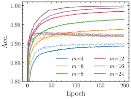
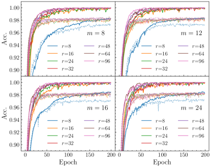
For the full TTN, the expressiveness of the classifier increases with increasing bond dimension $m$, as reflected by the improving training set accuracy. However, the model does not generalize well on the validation set as classifiers with $m>4$ all give approximately 92-93% validation set accuracy, well below the best training set accuracies. This is a typical feature of overfitting. In contrast, the low-rank TTN provide an implicit regularization, and the low-rank TTN classifiers are able to achieve 98.3% test accuracy. Importantly, the CP rank $r$ does not play a pivotal role in the performance as long as $r>m$. Similar to observations for low-rank tensor network state simulations of quantum systems in Ref. Chen2022_05 , $r\approx m$ seems sufficient for the low-rank TTN classifiers. In addition to the improved generalization properties, according to Eqs. (11) and (14), this implies substantial computation cost reductions.

IV Fashion-MNIST benchmark computations

As a second test, we compare full and low-rank TTN classifiers with branching ratios $b=2$ and $b=4$ for the more challenging Fashion-MNIST dataset Xiao2017_08 . It comprises 70 000 grayscale $28\times 28$ images for $L=10$ classes of clothing. We split the dataset in the same way as for MNIST and apply the same methods for image rescaling and TTN initialization.

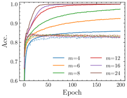
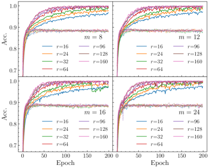
Training histories for full and low-rank TTN classifiers with branching ratio $b=4$ and $T=4$ layers are presented in Figs. 4 and 5. We find that the overfitting issue of the full TTN classifier is more prominent for Fashion-MNIST. As shown in Fig. 4, although networks with $m\geq 12$ can reach nearly 100% training set accuracy, their accuracies on the validation set reach only about 84%. Similar to the MNIST case, introducing the CP rank constraint on the TTN tensors substantially improves the generalization properties of the network. The low-rank TTN classifier achieves 88.5% classification accuracy on the test dataset.

Even for low-rank TTN, there is apparently still a considerable degree of overfitting. For almost all considered $m$ and $r$, the training set accuracy converges to almost 100%, but the validation set accuracy converges (much more quickly) to a value close to the aforementioned test set accuracy of 88.5%.

To further improve the generalization properties, we leverage the CP form (12) of the rank-constrained tensors and employ the tensor dropout method proposed in Ref. Kolbeinsson2021-15 based on similar approaches used in neural-network training Srivastava2014-15 : In the training phase, each component in the sum of Eq. (12) is associated with a Bernoulli random variable $\lambda^{\tau,k}_{i}$ taking value 1 with probability $1-p$ and 0 with probability $p$. Only the terms with $\lambda^{\tau,k}_{i}=1$ are retained, and the new tensors after the dropout operation are chosen as

$$\tilde{A}^{(\tau)}_{i}=\frac{1}{1-p}\,\sum_{k=1}^{r}\lambda^{\tau,k}_{i}\,\tilde{{\bm{a}}}^{\tau,k}_{i}\otimes{\bm{a}}^{\tau,k}_{i_{1}}\otimes\dotsb\otimes{\bm{a}}^{\tau,k}_{i_{b}}.$$ (16)

Figure 4: Fashion-MNIST training histories of full TTN classifiers with branching ratio $b=4$ and a few different bond dimensions $m$. Solid and dashed lines represent the classification accuracy (15) for the training set and validation set, respectively.

Figure 5: Fashion-MNIST training histories of low-rank TTN classifiers with branching ratio $b=4$, varying bond dimensions $m$, and CP ranks $r$. Solid and dashed lines represent the classification accuracy (15) for the training set and validation set, respectively.

We call $p$ the dropout rate. For each training iteration, the $\lambda^{\tau,k}_{i}$ are sampled from the Bernoulli distribution, the outputs ${\bm{f}}({\bm{x}}_{s})$ of the network are computed using the modified tensors (16), and the tensor parameters are updated accordingly using backpropagation algorithms. When the training is completed or its classification accuracy is tested, the tensor dropout operation is removed ($p=0$). In our implementation, we apply tensor dropout on all tensors except for the top tensor $A^{(T)}$.

Figure 6: Fashion-MNIST training histories of low-rank TTN classifiers with tensor dropout rate $p=0.2$ and branching ratio $b=4$. Solid and dashed lines are the classification accuracy (15) for the training set and validation set, respectively.

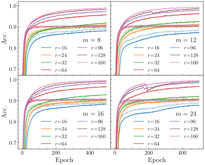
Figure 6 shows training histories for low-rank TTN classifiers with branching ratio $b=4$ and the tensor dropout regularization with rate $p=0.2$. Compared to the results without tensor dropout, training set accuracies now converge more slowly and display smaller fluctuations. Moreover, the classification accuracies for the validation set are improved by about 1-2%.

Figure 7b shows the dependence of the test set accuracy on the bond dimension $m$ and CP rank $r$ for the low-rank TTN with $b=4$ and dropout rate $p=0.2$. The classification accuracy increases rapidly when $m$ or $r$ is small and enters an extended plateau for $m\gtrsim 12$ and $r\gtrsim 32$. The best test set accuracy of 90.3% observed in these simulations occurs for $m=16$, $r=64$, and $p=0.3$.

To study the effect of the branching ratio $b$ on the classification accuracy of the low-rank TTN, we perform similar experiments with $b=2$. Compared to the $b=4$ networks, the number of layers doubles to $T=8$. During the training of TTN with large $m$ and $r$, we encountered some diverging vector components for the tensors (12). This can be explained by the fact that, for fixed network structure, $m$, and $r$, the set of low-rank TTN classifiers is generally not closed Bini1979-8 ; DeSilva2008-30 ; Barthel2022-112 . To avoid convergence to non-included boundary points of the set, which is associated with diverging vector elements, we add the penalty term $\gamma\sum_{\tau,i}\|A^{(\tau)}_{i}\|^{2}$ to the loss function (7) as suggested in Ref. Barthel2022-112 . Here, we choose $\gamma=0.01$. The results are shown in Fig. 7a. While the test set accuracy as a function of $m$ and $r$ displays a plateau similar to the case with branching ratio $b=4$, the test accuracy for $b=2$ is generally lower by around 4%.

Table 1: Test set accuracies of different image classifiers for the Fashion-MNIST dataset.

Model	Test Accuracy
MPSEfthymiou2019_06	88.0%
PEPS Cheng2021-103	88.3%
Low-rank TTN	88.5%
MPS+TTNStoudenmire2018-3	89.0%
XGBoostXiao2017_08	89.8%
AlexNetXiao2017_08	89.9%
Low-rank TTN (with tensor dropout)	90.3%
GoogLeNetXiao2017_08	93.7%

This can be attributed to the larger average graph distance of pixels in the TTN with smaller branching ratio $b$. As an example, features that depend on both the left and right halves of the image can only be detected by the top tensor, i.e., after seven layer transitions for $b=2$ but already after three layer transitions for $b=4$. The data in Fig. 7 confirms the benefits of large $b$, which can be achieved much more easily with the low-rank TTN classifiers.

Figure 7: Dependence of the Fashion-MNIST test set accuracy on the bond dimension $m$ and CP rank $r$ for low-rank TTN classifiers with branching ratio $b=2$ (left) and $b=4$ (right). The tensor dropout rate was set to $p=0.2$. To mitigate fluctuations of the test accuracy, at each point, we have averaged the results of five runs with different initial conditions. In both cases, the accuracy rapidly reaches a plateau, but the $b=4$ classifier clearly outperforms the one with $b=2$. Note the different accuracy scales and color scales in the two plots.

Figure 8: The Fashion-MNIST test set accuracy as a function of tensor dropout rate $p$ for various CP ranks $r$. Here we use branching ratio $b=4$ and bond dimension $m=16$.

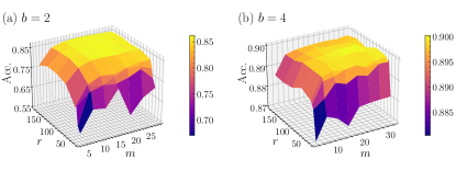
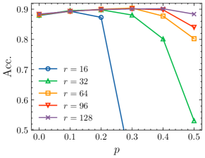
Figure 8 assesses the dependence of the test set accuracy on the dropout rate $p$. Starting from $p=0$, the curves for fixed $m=16$ and several $r$ all display a slow increase of the accuracy which is followed by a more rapid decrease at larger $p$. The turning point $p_{c}$ increases with increasing CP rank $r$, and networks with higher ranks are more robust in the sense that the final accuracy decrease for $p>p_{c}$ is not as drastic.

Finally, we compare our results with other state-of-the-art classification methods in Table 1. The low-rank TTN model with tensor dropout outperforms other tensor-network based approaches. Despite its simple structure and low computation costs, the low-rank TTN with tensor dropout is also competitive with more prominent machine-learning approaches like the convolutional-neural-network based AlexNet Krizhevsky2017-60 and the decision-tree based XGBoost Chen2016_08 .

V Discussion

The only nonlinear step in the TTN classifiers are the feature map (2) and the class label prediction (6). Also supported by the benchmark simulations, we expect that there is hence no vanishing gradient problem as encountered for neural networks Bengio1993-3 ; Hochreiter1998-06 ; Fukumizu2000-13 ; Dauphin2014-2 ; Shalev2017-70 . In fact, it has recently been shown that energy minimization problems for isometric tensor network optimization are free of barren plateaus for systems with finite-range interactions Barthel2023_03 ; Miao2023_04 ; Liu2022-129 . It is conceivable that this result can be extended to the image classification problem. To this purpose, one needs to assess locality properties of the corresponding loss functions such as the negative log-likelihood (7) or the structure of correlations in the optimized classifier, e.g., by studying entanglement properties Liu2019-21 ; Martyn2020_07 ; Liu2021-7 ; Convy2022-3a ; Dymarsky2022-4 .

On the other hand, having fewer non-linear elements may of course also reduce the expressiveness or generalization power. It would hence be interesting to combine the low-rank TTN weight tensor with more elaborate nonlinear feature maps. For example, it would be natural to employ $d$-dimensional feature vectors

$$\phi_{s}(x_{j})=\sqrt{\begin{pmatrix}d-1\\ s_{j}-1\end{pmatrix}}\left(\cos\frac{\pi x_{j}}{2}\right)^{d-s_{j}}\left(\sin\frac{\pi x_{j}}{2}\right)^{s_{j}-1},$$

with $s=1,\dotsc,d$ as suggested in Stoudenmire2016-29 . Here, we can increase from $d=2$, corresponding to Eq. (2), to $d\approx m$ without increasing the overall scaling of computation costs [Eqs. (11) and (14)].

Another simple route for improvements would be to employ a separate TTN for every class, i.e., to work with $L$ binary classifiers where the top tensor maps into $\mathbb{C}^{2}$ instead of $\mathbb{C}^{L}$ as done in Ref. Liu2019-21 .

A major advantage of the CP rank constraints in the low-rank TTN is that we can efficiently accommodate much larger tree branching rations $b$, compared to full TTN. In the presented benchmark simulations we only used $b\leq 4$ because of the small MNIST and Fashion-MNIST image sizes. We observed substantial accuracy gains when going from $b=2$ to $b=4$. It will hence be interesting to investigate the performance of low-rank TTN classifiers with even larger $b$ in more challenging machine learning problems.