${\rm AdANNS}$: A Framework for Adaptive Semantic Search

Abstract

Web-scale search systems learn an encoder to embed a given query which is then hooked into an approximate nearest neighbor search (ANNS) pipeline to retrieve similar data points. To accurately capture tail queries and data points, learned representations typically are rigid, high-dimensional vectors that are generally used as-is in the entire ANNS pipeline and can lead to computationally expensive retrieval. In this paper, we argue that instead of rigid representations, different stages of ANNS can leverage adaptive representations of varying capacities to achieve significantly better accuracy-compute trade-offs, i.e., stages of ANNS that can get away with more approximate computation should use a lower-capacity representation of the same data point. To this end, we introduce ${\rm AdANNS}$ , a novel ANNS design framework that explicitly leverages the flexibility of Matryoshka Representations [31]. We demonstrate state-of-the-art accuracy-compute trade-offs using novel ${\rm AdANNS}$-based key ANNS building blocks like search data structures (${\rm AdANNS}$-IVF) and quantization (${\rm AdANNS}$-OPQ). For example on ImageNet retrieval, ${\rm AdANNS}$-IVF is up to $\mathbf{1.5}\%$ more accurate than the rigid representations-based IVF [48] at the same compute budget; and matches accuracy while being up to $\mathbf{90}\times$ faster in wall-clock time. For Natural Questions, $32$-byte ${\rm AdANNS}$-OPQ matches the accuracy of the $64$-byte OPQ baseline [13] constructed using rigid representations – same accuracy at half the cost! We further show that the gains from ${\rm AdANNS}$ translate to modern-day composite ANNS indices that combine search structures and quantization. Finally, we demonstrate that ${\rm AdANNS}$ can enable inference-time adaptivity for compute-aware search on ANNS indices built non-adaptively on matryoshka representations. Code is open-sourced at https://github.com/RAIVNLab/AdANNS.

1 Introduction

Semantic search [24] on learned representations [40, 41, 50] is a major component in retrieval pipelines [4, 9]. In its simplest form, semantic search methods learn a neural network to embed queries as well as a large number ($N$) of data points in a $d$-dimensional vector space. For a given query, the nearest (in embedding space) point is retrieved using either an exact search or using approximate nearest neighbor search (ANNS) [21] which is now indispensable for real-time large-scale retrieval.

(a) Image retrieval on ImageNet-1K.

(b) Passage retrieval on Natural Questions.

Figure 1: ${\rm AdANNS}$ helps design search data structures and quantization methods with better accuracy-compute trade-offs than the existing solutions. In particular, (a) ${\rm AdANNS}$-IVF improves on standard IVF by up to $1.5\%$ in accuracy while being $90\times$ faster in deployment and (b) ${\rm AdANNS}$-OPQ is as accurate as the baseline at half the cost! Rigid-IVF and Rigid-OPQ are standard techniques that are built on rigid representations (${\rm RRs}$) while ${\rm AdANNS}$ uses matryoshka representations (${\rm MRs}$) [31].

Existing semantic search methods learn fixed or rigid representations (${\rm RRs}$) which are used as is in all the stages of ANNS (data structures for data pruning and quantization for cheaper distance computation; see Section 2). That is, while ANNS indices allow a variety of parameters for searching the design space to optimize the accuracy-compute trade-off, the provided data dimensionality is typically assumed to be an immutable parameter. To make it concrete, let us consider inverted file index (IVF) [48], a popular web-scale ANNS technique [16]. IVF has two stages (Section 3) during inference: (a) cluster mapping: mapping the query to a cluster of data points [36], and (b) linear scan: distance computation w.r.t all points in the retrieved cluster to find the nearest neighbor (NN). Standard IVF utilizes the same high-dimensional ${\rm RR}$ for both phases, which can be sub-optimal.

Why the sub-optimality? Imagine one needs to partition a dataset into $k$ clusters for IVF and the dimensionality of the data is $d$ – IVF uses full $d$ representation to partition into $k$ clusters. However, suppose we have an alternate approach that somehow projects the data in $d/2$ dimensions and learns $2k$ clusters. Note that the storage and computation to find the nearest cluster remains the same in both cases, i.e., when we have $k$ clusters of $d$ dimensions or $2k$ clusters of $d/2$ dimensions. $2k$ clusters can provide significantly more refined partitioning, but the distances computed between queries and clusters could be significantly more inaccurate after projection to $d/2$ dimensions.

So, if we can find a mechanism to obtain a $d/2$-dimensional representation of points that can accurately approximate the topology/distances of $d$-dimensional representation, then we can potentially build significantly better ANNS structure that utilizes different capacity representations for the cluster mapping and linear scan phases of IVF. But how do we find such adaptive representations? These desired adaptive representations should be cheap to obtain and still ensure distance preservation across dimensionality. Post-hoc dimensionality reduction techniques like SVD [14] and random projections [25] on high-dimensional ${\rm RRs}$ are potential candidates, but our experiments indicate that in practice they are highly inaccurate and do not preserve distances well enough (Figure 2).

Instead, we identify that the recently proposed Matryoshka Representations (${\rm MRs}$) [31] satisfy the specifications for adaptive representations. Matryoshka representations pack information in a hierarchical nested manner, i.e., the first $m$-dimensions of the $d$-dimensional ${\rm MR}$ form an accurate low-dimensional representation while being aware of the information in the higher dimensions. This allows us to deploy ${\rm MRs}$ in two major and novel ways as part of ANNS: (a) low-dimensional representations for accuracy-compute optimal clustering and quantization, and (b) high-dimensional representations for precise re-ranking when feasible.

To this effort, we introduce ${\rm AdANNS}$ , a novel design framework for semantic search that uses matryoshka representation-based adaptive representations across different stages of ANNS to ensure significantly better accuracy-compute trade-off than the state-of-the-art baselines.

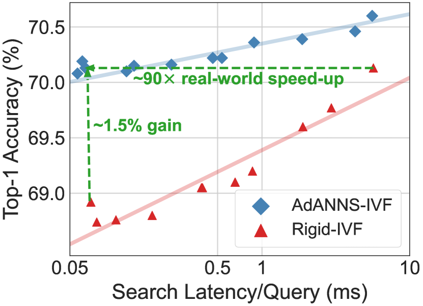
Typical ANNS systems have two key components: (a) search data structure to store datapoints, (b) distance computation to map a given query to points in the data structure. Through ${\rm AdANNS}$, we address both these components and significantly improve their performance. In particular, we first propose ${\rm AdANNS}$-IVF (Section 4.1) which tackles the first component of ANNS systems. ${\rm AdANNS}$-IVF uses standard full-precision computations but uses adaptive representations for different IVF stages. On ImageNet 1-NN image retrieval (Figure 1(a)), ${\rm AdANNS}$-IVF is up to $1.5\%$ more accurate for the compute budget and $90\times$ cheaper in deployment for the same accuracy as IVF.

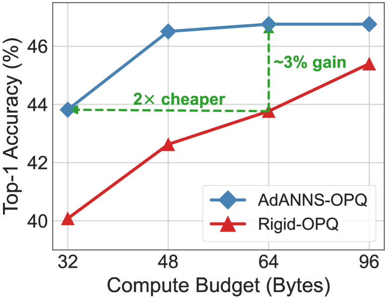
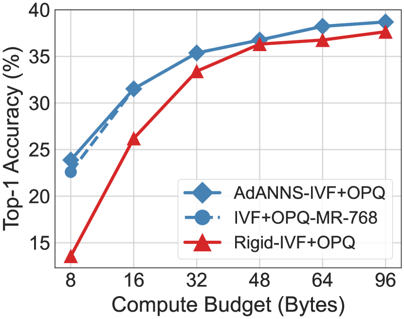
We then propose ${\rm AdANNS}$-OPQ (Section 4.2) which addresses the second component by using ${\rm AdANNS}$-based quantization (OPQ [13]) – here we use exhaustive search overall points. ${\rm AdANNS}$-OPQ is as accurate as the baseline OPQ on ${\rm RRs}$ while being at least $\mathbf{2\times}$ faster on Natural Questions [32] 1-NN passage retrieval (Figure 1(b)). Finally, we combine the two techniques to obtain ${\rm AdANNS}$-IVFOPQ (Section 4.3) which is more accurate while being much cheaper – up to $\mathbf{8\times}$ – than the traditional IVFOPQ [24] index. To demonstrate generality of our technique, we adapt ${\rm AdANNS}$ to DiskANN [22] which provides interesting accuracy-compute tradeoff; see Table 4.3.

While ${\rm MR}$ already has multi-granular representations, careful integration with ANNS building blocks is critical to obtain a practical method and is our main contribution. In fact, Kusupati et al. [31] proposed a simple adaptive retrieval setup that uses smaller-dimensional ${\rm MR}$ for shortlisting in retrieval followed by precise re-ranking with a higher-dimensional ${\rm MR}$. Such techniques, unfortunately, cannot be scaled to industrial systems as they require forming a new index for every shortlisting provided by low-dimensional ${\rm MR}$. Ensuring that the method aligns well with the modern-day ANNS pipelines is important as they already have mechanisms to handle real-world constraints like load-balancing [16] and random access from disk [22]. So, ${\rm AdANNS}$ is a step towards making the abstraction of adaptive search and retrieval feasible at the web-scale.

Through extensive experimentation, we also show that ${\rm AdANNS}$ generalizes across search data structures, distance approximations, modalities (text & image), and encoders (CNNs & Transformers) while still translating the theoretical gains to latency reductions in deployment. While we have mainly focused on IVF and OPQ-based ANNS in this work, ${\rm AdANNS}$ also blends well with other ANNS pipelines. We also show that ${\rm AdANNS}$ can enable compute-aware elastic search on prebuilt indices without making any modifications (Section 5.1); note that this is in contrast to ${\rm AdANNS}$-IVF that builds the index explicitly utilizing “adaptivity” in representations. Finally, we provide an extensive analysis on the alignment of matryoshka representation for better semantic search (Section 5.2).

We make the following key contributions:

• We introduce ${\rm AdANNS}$ , a novel framework for semantic search that leverages matryoshka representations for designing ANNS systems with better accuracy-compute trade-offs.

• ${\rm AdANNS}$ powered search data structure (${\rm AdANNS}$-IVF) and quantization (${\rm AdANNS}$-OPQ) show a significant improvement in accuracy-compute tradeoff compared to existing solutions.

• ${\rm AdANNS}$ generalizes to modern-day composite ANNS indices and can also enable compute-aware elastic search during inference with no modifications.

2 Related Work

Approximate nearest neighbour search (ANNS) is a paradigm to come as close as possible [7] to retrieving the “true” nearest neighbor (NN) without the exorbitant search costs associated with exhaustive search [21, 52]. The “approximate” nature comes from data pruning as well as the cheaper distance computation that enable real-time web-scale search. In its naive form, NN-search has a complexity of $\mathcal{O}(dN)$; $d$ is the data dimensionality used for distance computation and $N$ is the size of the database. ANNS employs each of these approximations to reduce the linear dependence on the dimensionality (cheaper distance computation) and data points visited during search (data pruning).

Cheaper distance computation. From a bird’s eye view, cheaper distance computation is always obtained through dimensionality reduction (quantization included). PCA and SVD [14, 26] can reduce dimensionality and preserve distances only to a limited extent without sacrificing accuracy. On the other hand, quantization-based techniques [6, 15] like (optimized) product quantization ((O)PQ) [13, 23] have proved extremely crucial for relatively accurate yet cheap distance computation and simultaneously reduce the memory overhead significantly. Another naive solution is to independently train the representation function with varying low-dimensional information bottlenecks [31] which is rarely used due to the costs of maintaining multiple models and databases.

Data pruning. Enabled by various data structures, data pruning reduces the number of data points visited as part of the search. This is often achieved through hashing [8, 46], trees [3, 12, 16, 48] and graphs [22, 38]. More recently there have been efforts towards end-to-end learning of the search data structures [17, 29, 30]. However, web-scale ANNS indices are often constructed on rigid $d$-dimensional real vectors using the aforementioned data structures that assist with the real-time search. For a more comprehensive review of ANNS structures please refer to [5, 34, 51].

Composite indices. ANNS pipelines often benefit from the complementary nature of various building blocks [24, 42]. In practice, often the data structures (coarse-quantizer) like IVF [48] and HNSW [37] are combined with cheaper distance alternatives like PQ [23] (fine-quantizer) for massive speed-ups in web-scale search. While the data structures are built on $d$-dimensional real vectors, past works consistently show that PQ can be safely used for distance computation during search time. As evident in modern web-scale ANNS systems like DiskANN [22], the data structures are built on $d$-dimensional real vectors but work with PQ vectors ($32-64$-byte) for fast distance computations.

ANNS benchmark datasets. Despite the Herculean advances in representation learning [19, 42], ANNS progress is often only benchmarked on fixed representation vectors provided for about a dozen million to billion scale datasets [1, 47] with limited access to the raw data. This resulted in the improvement of algorithmic design for rigid representations (${\rm RRs}$) that are often not specifically designed for search. All the existing ANNS methods work with the assumption of using the provided $d$-dimensional representation which might not be Pareto-optimal for the accuracy-compute trade-off in the first place. Note that the lack of raw-image and text-based benchmarks led us to using ImageNet-1K [45] (1.3M images, 50K queries) and Natural Questions [32] (21M passages, 3.6K queries) for experimentation. While not billion-scale, the results observed on ImageNet often translate to real-world progress [28], and Natural Questions is one of the largest question answering datasets benchmarked for dense passage retrieval [27], making our results generalizable and widely applicable.

In this paper, we investigate the utility of adaptive representations – embeddings of different dimensionalities having similar semantic information – in improving the design of ANNS algorithms. This helps in transitioning out of restricted construction and inference on rigid representations for ANNS. To this end, we extensively use Matryoshka Representations (${\rm MRs}$) [31] which have desired adaptive properties in-built. To the best of our knowledge, this is the first work that improves accuracy-compute trade-off in ANNS by leveraging adaptive representations on different phases of construction and inference for ANNS data structures.

3 Problem Setup, Notation, and Preliminaries

The problem setup of approximate nearest neighbor search (ANNS) [21] consists of a database of $N$ data points, $[x_{1},x_{2},\ldots,x_{N}]$, and a query, $q$, where the goal is to “approximately” retrieve the nearest data point to the query. Both the database and query are embedded to $\mathbb{R}^{d}$ using a representation function $\phi:\mathcal{X}\to\mathbb{R}^{d}$, often a neural network that can be learned through various representation learning paradigms [2, 19, 20, 40, 42].

Matryoshka Representations (${\rm MRs}$).

The $d$-dimensional representations from $\phi$ can have a nested structure like Matryoshka Representations (${\rm MRs}$) [31] in-built – $\phi^{\textsc{MR}(d)}$. Matryoshka Representation Learning (MRL) learns these nested representations with a simple strategy of optimizing the same training objective at varying dimensionalities. These granularities are ordered such that the lowest representation size forms a prefix for the higher-dimensional representations. So, high-dimensional ${\rm MR}$ inherently contains low-dimensional representations of varying granularities that can be accessed for free – first $m$-dimensions ($m\in[d]$) ie., $\phi^{\textsc{MR}(d)}[1:m]$ from the $d$-dimensional ${\rm MR}$ form an $m$-dimensional representation which is as accurate as its independently trained rigid representation (${\rm RR}$) counterpart – $\phi^{\textsc{RR}(m)}$. Training an encoder with MRL does not involve any overhead or hyperparameter tuning and works seamlessly across modalities, training objectives, and architectures.

Inverted File Index (IVF).

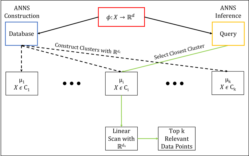
IVF [48] is an ANNS data structure used in web-scale search systems [16] owing to its simplicity, minimal compute overhead, and high accuracy. IVF construction involves clustering (coarse quantization through k-means) [36] on $d$-dimensional representation that results in an inverted file list [53] of all the data points in each cluster. During search, $d$-dimensional query representation is assigned to the most relevant cluster ($C_{i}$; $i\in[k]$) by finding the closest centroid ($\mu_{i}$) using an appropriate distance metric ($L_{2}$ or cosine). This is followed by an exhaustive linear search across all data points in the cluster which gives the closest NN (see Figure 5 in Appendix A for IVF overview). Lastly, IVF can scale to web-scale by utilizing a hierarchical IVF structure within each cluster [16]. Table 2 in Appendix A describes the retrieval formula for multiple variants of IVF.

Optimized Product Quantization (OPQ).

Product Quantization (PQ) [23] works by splitting a $d$-dimensional real vector into $m$ sub-vectors and quantizing each sub-vector with an independent $2^{b}$ length codebook across the database. After PQ, each $d$-dimensional vector can be represented by a compact $m\times b$ bit vector; we make each vector $m$ bytes long by fixing $b=8$. During search time, distance computation between the query vector and PQ database is extremely efficient with only $m$ codebook lookups. The generality of PQ encompasses scalar/vector quantization [15, 36] as special cases. However, PQ can be further improved by rotating the $d$-dimensional space appropriately to maximize distance preservation after PQ. Optimized Product Quantization (OPQ) [13] achieves this by learning an orthonormal projection matrix $R$ that rotates the $d$-dimensional space to be more amenable to PQ. OPQ shows consistent gains over PQ across a variety of ANNS tasks and has become the default choice in standard composite indices [22, 24].

Datasets.

We evaluate the ANNS algorithms while changing the representations used for the search thus making it impossible to evaluate on the usual benchmarks [1]. Hence we experiment with two public datasets: (a) ImageNet-1K [45] dataset on the task of image retrieval – where the goal is to retrieve images from a database (1.3M image train set) belonging to the same class as the query image (50K image validation set) and (b) Natural Questions (NQ) [32] dataset on the task of question answering through dense passage retrieval – where the goal is to retrieve the relevant passage from a database (21M Wikipedia passages) for a query (3.6K questions).

Metrics

Performance of ANNS is often measured using recall score [22], $k$-recall@$N$ – recall of the exact NN across search complexities which denotes the recall of $k$ “true” NN when $N$ data points are retrieved. However, the presence of labels allows us to compute 1-NN (top-1) accuracy. Top-1 accuracy is a harder and more fine-grained metric that correlates well with typical retrieval metrics like recall and mean average precision (mAP@$k$). Even though we report top-1 accuracy by default during experimentation, we discuss other metrics in Appendix C. Finally, we measure the compute overhead of ANNS using MFLOPS/query and also provide wall-clock times (see Appendix B.1).

Encoders.

For ImageNet, we encode both the database and query set using a ResNet50 ($\phi_{I}$) [19] trained on ImageNet-1K. For NQ, we encode both the passages in the database and the questions in the query set using a BERT-Base ($\phi_{N}$) [10] model fine-tuned on NQ for dense passage retrieval [27].

We use the trained ResNet50 models with varying representation sizes ($d=[8,16,\dots,2048]$; default being $2048$) as suggested by Kusupati et al. [31] alongside the MRL-ResNet50 models trained with MRL for the same dimensionalities. The ${\rm RR}$ and ${\rm MR}$ models are trained to ensure the supervised one-vs-all classification accuracy across all data dimensionalities is nearly the same – 1-NN accuracy of $2048$-$d$ ${\rm RR}$ and ${\rm MR}$ models are $71.19\%$ and $70.97\%$ respectively on ImageNet-1K. Independently trained models, $\phi_{I}^{\textsc{RR}(d)}$, output $d=[8,16\ldots,2048]$ dimensional ${\rm RRs}$ while a single MRL-ResNet50 model, $\phi_{I}^{\textsc{MR}(d)}$, outputs a $d=2048$-dimensional ${\rm MR}$ that contains all the 9 granularities.

We also train BERT-Base models in a similar vein as the aforementioned ResNet50 models. The key difference is that we take a pre-trained BERT-Base model and fine-tune on NQ as suggested by Karpukhin et al. [27] with varying (5) representation sizes (bottlenecks) ($d=[48,96,\dots,768]$; default being $768$) to obtain $\phi_{N}^{\textsc{RR}(d)}$ that creates ${\rm RRs}$ for the NQ dataset. To get the MRL-BERT-Base model, we fine-tune a pre-trained BERT-Base encoder on the NQ train dataset using the MRL objective with the same granularities as ${\rm RRs}$ to obtain $\phi_{N}^{\textsc{MR}(d)}$ which contains all five granularities. Akin to ResNet50 models, the ${\rm RR}$ and ${\rm MR}$ BERT-Base models on NQ are built to have similar 1-NN accuracy for $768$-$d$ of $52.2\%$ and $51.5\%$ respectively. More implementation details can be found in Appendix B and additional experiment-specific information is provided at the appropriate places.

4 ${\rm AdANNS}$ – Adaptive ANNS

In this section, we present our proposed ${\rm AdANNS}$  framework that exploits the inherent flexibility of matryoshka representations to improve the accuracy-compute trade-off for semantic search components. Standard ANNS pipeline can be split into two key components: (a) search data structure that indexes and stores data points, (b) query-point computation method that outputs (approximate) distance between a given query and data point. For example, standard IVFOPQ [24] method uses an IVF structure to index points on full-precision vectors and then relies on OPQ for more efficient distance computation between the query and the data points during the linear scan.

Below, we show that ${\rm AdANNS}$ can be applied to both the above-mentioned ANNS components and provides significant gains on the computation-accuracy tradeoff curve. In particular, we present ${\rm AdANNS}$-IVF which is ${\rm AdANNS}$ version of the standard IVF index structure [48], and the closely related ScaNN structure [16]. We also present ${\rm AdANNS}$-OPQ which introduces representation adaptivity in the OPQ, an industry-default quantization. Then, in Section 4.3 we further demonstrate the combination of the two techniques to get ${\rm AdANNS}$-IVFOPQ – an ${\rm AdANNS}$ version of IVFOPQ [24] – and ${\rm AdANNS}$-DiskANN, a similar variant of DiskANN [22]. Overall, our experiments show that ${\rm AdANNS}$-IVF is significantly more accuracy-compute optimal compared to the IVF indices built on ${\rm RRs}$ and ${\rm AdANNS}$-OPQ is as accurate as the OPQ on ${\rm RRs}$ while being significantly cheaper.

4.1 ${\rm AdANNS}$-IVF

Figure 2: 1-NN accuracy on ImageNet retrieval shows that ${\rm AdANNS}$-IVF achieves near-optimal accuracy-compute trade-off compared across various rigid and adaptive baselines. Both adaptive variants of ${\rm MR}$ and ${\rm RR}$ significantly outperform their rigid counterparts (IVF-XX) while post-hoc compression on ${\rm RR}$ using SVD for adaptivity falls short.

Recall from Section 1 that IVF has a clustering and a linear scan phase, where both phase use same dimensional rigid representation. Now, ${\rm AdANNS}$-IVF allows the clustering phase to use the first $d_{c}$ dimensions of the given matryoshka representation (${\rm MR}$). Similarly, the linear scan within each cluster uses $d_{s}$ dimensions, where again $d_{s}$ represents top $d_{s}$ coordinates from ${\rm MR}$. Note that setting $d_{c}=d_{s}$ results in non-adaptive regular IVF. Intuitively, we would set $d_{c}\ll d_{s}$, so that instead of clustering with a high-dimensional representation, we can approximate it accurately with a low-dimensional embedding of size $d_{c}$ followed by a linear scan with a higher $d_{s}$-dimensional representation. Intuitively, this helps in the smooth search of design space for state-of-the-art accuracy-compute trade-off. Furthermore, this can provide a precise operating point on accuracy-compute tradeoff curve which is critical in several practical settings.

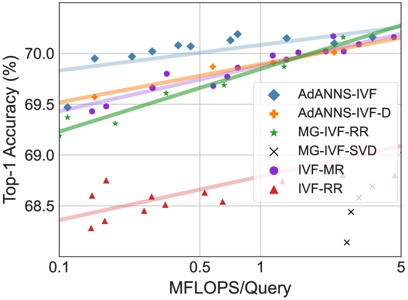
Our experiments on regular IVF with ${\rm MRs}$ and ${\rm RRs}$ (IVF-${\rm MR}$ & IVF-${\rm RR}$) of varying dimensionalities and IVF configurations (# clusters, # probes) show that (Figure 2) matryoshka representations result in a significantly better accuracy-compute trade-off. We further studied and found that learned lower-dimensional representations offer better accuracy-compute trade-offs for IVF than higher-dimensional embeddings (see Appendix E for more results).

${\rm AdANNS}$ utilizes $d$-dimensional matryoshka representation to get accurate $d_{c}$ and $d_{s}$ dimensional vectors at no extra compute cost. The resulting ${\rm AdANNS}$-IVF provides a much better accuracy-compute trade-off (Figure 2) on ImageNet-1K retrieval compared to IVF-${\rm MR}$, IVF-${\rm RR}$, and MG-IVF-${\rm RR}$ – multi-granular IVF with rigid representations (akin to ${\rm AdANNS}$ without ${\rm MR}$) – a strong baseline that uses $d_{c}$ and $d_{s}$ dimensional ${\rm RRs}$. Finally, we exhaustively search the design space of IVF by varying $d_{c},d_{s}\in[8,16,\ldots,2048]$ and the number of clusters $k\in[8,16,\ldots,2048]$. Please see Appendix E for more details. For IVF experiments on the NQ dataset, please refer to Appendix G.

Empirical results.

Figure 2 shows that ${\rm AdANNS}$-IVF outperforms the baselines across all accuracy-compute settings for ImageNet-1K retrieval. ${\rm AdANNS}$-IVF results in $10\times$ lower compute for the best accuracy of the extremely expensive MG-IVF-${\rm RR}$ and non-adaptive IVF-${\rm MR}$. Specifically, as shown in Figure 1(a), ${\rm AdANNS}$-IVF is up to $1.5\%$ more accurate for the same compute and has up to $100\times$ lesser FLOPS/query ($90\times$ real-world speed-up!) than the status quo ANNS on rigid representations (IVF-${\rm RR}$). We filter out points for the sake of presentation and encourage the reader to check out Figure 8 in Appendix E for an expansive plot of all the configurations searched.

The advantage of ${\rm AdANNS}$ for construction of search structures is evident from the improvements in IVF (${\rm AdANNS}$-IVF) and can be easily extended to other ANNS structures like ScaNN [16] and HNSW [38]. For example, HNSW consists of multiple layers with graphs of NSW graphs [37] of increasing complexity. ${\rm AdANNS}$ can be adopted to HNSW, where the construction of each level can be powered by appropriate dimensionalities for an optimal accuracy-compute trade-off. In general, ${\rm AdANNS}$ provides fine-grained control over compute overhead (storage, working memory, inference, and construction cost) during construction and inference while providing the best possible accuracy.

4.2 ${\rm AdANNS}$-OPQ

Standard Product Quantization (PQ) essentially performs block-wise vector quantization via clustering. For example, suppose we need $32$-byte PQ compressed vectors from the given $2048$ dimensional representations. Then, we can chunk the representations in $m=32$ equal blocks/sub-vectors of $64$-d each, and each sub-vector space is clustered into $2^{8}=256$ partitions. That is, the representation of each point is essentially cluster-id for each block. Optimized PQ (OPQ) [13] further refines this idea, by first rotating the representations using a learned orthogonal matrix, and then applying PQ on top of the rotated representations. In ANNS, OPQ is used extensively to compress vectors and improves approximate distance computation primarily due to significantly lower memory overhead than storing full-precision data points IVF.

${\rm AdANNS}$-OPQ utilizes ${\rm MR}$ representations to apply OPQ on lower-dimensional representations. That is, for a given quantization budget, ${\rm AdANNS}$ allows using top $d_{s}\ll d$ dimensions from ${\rm MR}$ and then computing clusters with $d_{s}/m$-dimensional blocks where $m$ is the number of blocks. Depending on $d_{s}$ and $m$, we have further flexibility of trading-off dimensionality/capacity for increasing the number of clusters to meet the given quantization budget. ${\rm AdANNS}$-OPQ tries multiple $d_{s}$, $m$, and number of clusters for a fixed quantization budget to obtain the best performing configuration.

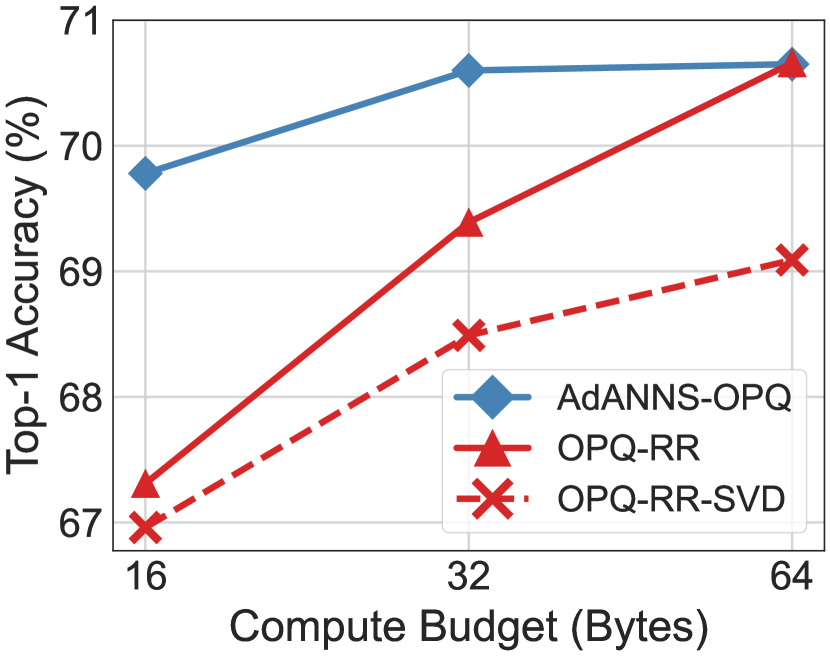
We experimented with $8-128$ byte OPQ budgets for both ImageNet and Natural Questions retrieval with an exhaustive search on the quantized vectors. We compare ${\rm AdANNS}$-OPQ which uses ${\rm MRs}$ of varying granularities to the baseline OPQ built on the highest dimensional ${\rm RRs}$. We also evaluate OPQ vectors obtained projection using SVD [14] on top of the highest-dimensional ${\rm RRs}$.

Figure 3: ${\rm AdANNS}$-OPQ matches the accuracy of $64$-byte OPQ on ${\rm RR}$ using only $32$-bytes for ImageNet retrieval. ${\rm AdANNS}$ provides large gains at lower compute budgets and saturates to baseline performance for larger budgets.

Figure 4: Combining the gains of ${\rm AdANNS}$ for IVF and OPQ leads to better IVFOPQ composite indices. On ImageNet retrieval, ${\rm AdANNS}$-IVFOPQ is 8$\times$ cheaper for the same accuracy and provides $1$ - $4\%$ gains over IVFOPQ on ${\rm RRs}$.

Empirical results.

Figures 4 and 1(b) show that ${\rm AdANNS}$-OPQ significantly outperforms – up to $4\%$ accuracy gain – the baselines (OPQ on ${\rm RRs}$) across compute budgets on both ImageNet and NQ. In particular, ${\rm AdANNS}$-OPQ tends to match the accuracy of a $64$-byte (a typical choice in ANNS) OPQ baseline with only a $32$-byte budget. This results in a $2\times$ reduction in both storage and compute FLOPS which translates to significant gains in real-world web-scale deployment (see Appendix D).

We only report the best ${\rm AdANNS}$-OPQ for each budget typically obtained through a much lower-dimensional ${\rm MR}$ ($128$ & $192$; much faster to build as well) than the highest-dimensional ${\rm MR}$ ($2048$ & $768$) for ImageNet and NQ respectively (see Appendix G for more details). At the same time, we note that building compressed OPQ vectors on projected ${\rm RRs}$ using SVD to the smaller dimensions (or using low-dimensional ${\rm RRs}$, see Appendix D) as the optimal ${\rm AdANNS}$-OPQ does not help in improving the accuracy. The significant gains we observe in ${\rm AdANNS}$-OPQ are purely due to better information packing in ${\rm MRs}$ – we hypothesize that packing the most important information in the initial coordinates results in a better PQ quantization than ${\rm RRs}$ where the information is uniformly distributed across all the dimensions [31, 49]. See Appendix D for more details and experiments.

4.3 ${\rm AdANNS}$ for Composite Indices

We now extend ${\rm AdANNS}$ to composite indices [24] which put together two main ANNS building blocks – search structures and quantization – together to obtain efficient web-scale ANNS indices used in practice. A simple instantiation of a composite index would be the combination of IVF and OPQ – IVFOPQ – where the clustering in IVF happens with full-precision real vectors but the linear scan within each cluster is approximated using OPQ-compressed variants of the representation – since often the full-precision vectors of the database cannot fit in RAM. Contemporary ANNS indices like DiskANN [22] make this a default choice where they build the search graph with a full-precision vector and approximate the distance computations during search with an OPQ-compressed vector to obtain a very small shortlist of retrieved datapoints. In DiskANN, the shortlist of data points is then re-ranked to form the final list using their full-precision vectors fetched from the disk. ${\rm AdANNS}$ is naturally suited to this shortlist-rerank framework: we use a low-$d$ ${\rm MR}$ for forming index, where we could tune ${\rm AdANNS}$ parameters according to the accuracy-compute trade-off of the graph and OPQ vectors. We then use a high-$d$ ${\rm MR}$ for re-ranking.

Empirical results.

Table 1: ${\rm AdANNS}$-DiskANN using a $16$-$d$ ${\rm MR}$ $+$ re-ranking with the $2048$-$d$ ${\rm MR}$ outperforms DiskANN built on $2048$-$d$ ${\rm RR}$ at half the compute cost on ImageNet retrieval.

	${\rm RR}$-2048	${\rm AdANNS}$
PQ Budget (Bytes)	32	16
Top-1 Accuracy (%)	70.37	70.56
mAP@10 (%)	62.46	64.70
Precision@40 (%)	65.65	68.25

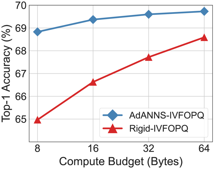
Figure 4 shows that ${\rm AdANNS}$-IVFOPQ is $1-4\%$ better than the baseline at all the PQ compute budgets. Furthermore, ${\rm AdANNS}$-IVFOPQ has the same accuracy as the baselines at $8\times$ lower overhead. With DiskANN, ${\rm AdANNS}$ accelerates shortlist generation by using low-dimensional representations and recoups the accuracy by re-ranking with the highest-dimensional ${\rm MR}$ at negligible cost. Table 4.3 shows that ${\rm AdANNS}$-DiskANN is more accurate than the baseline for both 1-NN and ranking performance at only $half$ the cost. Using low-dimensional representations further speeds up inference in ${\rm AdANNS}$-DiskANN (see Appendix F).

These results show the generality of ${\rm AdANNS}$ and its broad applicability across a variety of ANNS indices built on top of the base building blocks. Currently, ${\rm AdANNS}$ piggybacks on typical ANNS pipelines for their inherent accounting of the real-world system constraints [16, 22, 25]. However, we believe that ${\rm AdANNS}$’s flexibility and significantly better accuracy-compute trade-off can be further informed by real-world deployment constraints. We leave this high-potential line of work that requires extensive study to future research.

5 Further Analysis and Discussion

5.1 Compute-aware Elastic Search During Inference

${\rm AdANNS}$ search structures cater to many specific large-scale use scenarios that need to satisfy precise resource constraints during construction as well as inference. However, in many cases, construction and storage of the indices are not the bottlenecks or the user is unable to search the design space. In these settings, ${\rm AdANNS}$-D enables adaptive inference through accurate yet cheaper distance computation using the low-dimensional prefix of matryoshka representation. Akin to composite indices (Section 4.3) that use PQ vectors for cheaper distance computation, we can use the low-dimensional ${\rm MR}$ for faster distance computation on ANNS structure built non-adaptively with a high-dimensional ${\rm MR}$ without any modifications to the existing index.

Empirical results.

Figure 2 shows that for a given compute budget using IVF on ImageNet-1K retrieval, ${\rm AdANNS}$-IVF is better than ${\rm AdANNS}$-IVF-D due to the explicit control during the building of the ANNS structure which is expected. However, the interesting observation is that ${\rm AdANNS}$-D matches or outperforms the IVF indices built with ${\rm MRs}$ of varying capacities for ImageNet retrieval.

However, these methods are applicable in specific scenarios of deployment. Obtaining optimal ${\rm AdANNS}$ search structure (highly accurate) or even the best IVF-MR index relies on a relatively expensive design search but delivers indices that fit the storage, memory, compute, and accuracy constraints all at once. On the other hand ${\rm AdANNS}$-D does not require a precisely built ANNS index but can enable compute-aware search during inference. ${\rm AdANNS}$-D is a great choice for setups that can afford only one single database/index but need to cater to varying deployment constraints, e.g., one task requires 70% accuracy while another task has a compute budget of 1 MFLOPS/query.

5.2 Why ${\rm MRs}$ over ${\rm RRs}$?

Quite a few of the gains from ${\rm AdANNS}$ are owing to the quality and capabilities of matryoshka representations. So, we conducted extensive analysis to understand why matryoshka representations seem to be more aligned for semantic search than the status-quo rigid representations.

Difficulty of NN search. Relative contrast ($C_{r}$) [18] is inversely proportional to the difficulty of nearest neighbor search on a given database. On ImageNet-1K, Figure 14 shows that ${\rm MRs}$ have better $C_{r}$ than ${\rm RRs}$ across dimensionalities, further supporting that matryoshka representations are more aligned (easier) for NN search than existing rigid representations for the same accuracy. More details and analysis about this experiment can be found in Appendix H.2.

Clustering distributions. We also investigate the potential deviation in clustering distributions for ${\rm MRs}$ across dimensionalities compared to ${\rm RRs}$. Unlike the ${\rm RRs}$ where the information is uniformly diffused across dimensions [49], ${\rm MRs}$ have hierarchical information packing. Figure 11 in Appendix E.3 shows that matryoshka representations result in clusters similar (measured by total variation distance [33]) to that of rigid representations and do not result in any unusual artifacts.

Robustness. Figure 9 in Appendix E shows that ${\rm MRs}$ continue to be better than ${\rm RRs}$ even for out-of-distribution (OOD) image queries (ImageNetV2 [44]) using ANNS. It also shows that the highest data dimensionality need not always be the most robust which is further supported by the higher recall using lower dimensions. Further details about this experiment can be found in Appendix E.1.

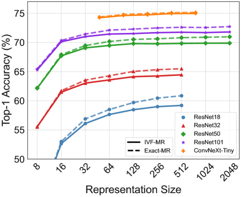
Generality across encoders. IVF-${\rm MR}$ consistently has higher accuracy than IVF-${\rm RR}$ across dimensionalities despite having similar accuracies with exact NN search (for ResNet50 on ImageNet and BERT-Base on NQ). We find that our observations on better alignment of ${\rm MRs}$ for NN search hold across neural network architectures, ResNet18/34/101 [19] and ConvNeXt-Tiny [35]. Appendix H.3 delves deep into the experimentation done using various neural architectures on ImageNet-1K.

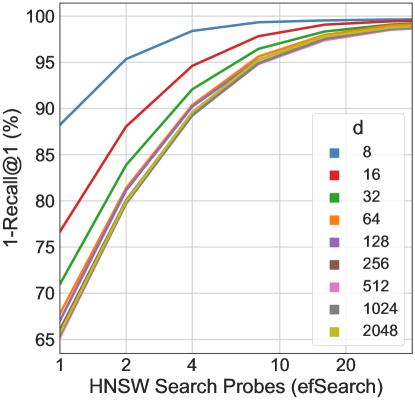
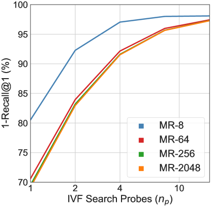
Recall score analysis. Analysis of recall score (see Appendix C) in Appendix H.1 shows that for a similar top-1 accuracy, lower-dimensional representations have better 1-Recall@1 across search complexities for IVF and HNSW on ImageNet-1K. Across the board, ${\rm MRs}$ have higher recall scores and top-1 accuracy pointing to easier “searchability” and thus suitability of matryoshka representations for ANNS. Larger-scale experiments and further analysis can be found in Appendix H.

Through these analyses, we argue that matryoshka representations are better suited for semantic search than rigid representations, thus making them an ideal choice for ${\rm AdANNS}$.

5.3 Search for ${\rm AdANNS}$ Hyperparameters

Choosing the optimal hyperparameters for AdANNS, such as $d_{c}$, $d_{s}$, $m$, # clusters, # probes, is an interesting and open problem that requires more rigorous examination. As the ANNS index is formed once and used for potentially billions of queries with massive implications for cost, latency and queries-per-second, a hyperparameter search for the best index is generally an acceptable industry practice [22, 38]. The Faiss library [24] provides guidelines to choose the appropriate index for a specific problem, including memory constraints, database size, and the need for exact results. There have been efforts at automating the search for optimal indexing parameters, such as Autofaiss, which maximizes recall given compute constraints.

In case of ${\rm AdANNS}$, we suggest starting at the best configurations of ${\rm MRs}$ followed by a local design space search to lead to near-optimal ${\rm AdANNS}$ configurations (e.g. use IVF-MR to bootstrap ${\rm AdANNS}$-IVF). We also share some observations during the course of our experiments:

1. ${\rm AdANNS}$-IVF: Top-1 accuracy generally improves (with diminishing returns after a point) with increasing dimensionality of clustering ($d_{c}$) and search ($d_{s}$), as we show on ImageNet variants and with multiple encoders in the Appendix (Figures 9 and 15). Clustering with low-$d$ ${\rm MRs}$ matches the performance of high-$d$ ${\rm MRs}$ as they likely contain similar amounts of useful information, making the increased compute cost not worth the marginal gains. Increasing # probes naturally boosts performance (Appendix, Figure 10(a)). Lastly, it is generally accepted that a good starting point for the # clusters $k$ is $\sqrt{N_{D}/2}$, where $N_{D}$ is the number of indexable items [39]. $k=\sqrt{N_{D}}$ is the optimal choice of $k$ from a FLOPS computation perspective as can be seen in Appendix B.1.

2. ${\rm AdANNS}$-OPQ: we observe that for a fixed compute budget in bytes ($m$), the top-1 accuracy reaches a peak at $d<d_{max}$ (Appendix, Table 4). We hypothesize that the better performance of ${\rm AdANNS}$-OPQ at $d<d_{max}$ is due to the curse of dimensionality, i.e. it is easier to learn PQ codebooks on smaller embeddings with similar amounts of information. We find that using an ${\rm MR}$ with $d=4\times m$ is a good starting point on ImageNet and NQ. We also suggest using an 8-bit (256-length) codebook for OPQ as the default for each of the sub-block quantizer.

3. ${\rm AdANNS}$-DiskANN: Our observations with DiskANN are consistent with other indexing structures, i.e. the optimal graph construction dimensionality $d<d_{max}$ (Appendix, Figure 12). A careful study of DiskANN on different datasets is required for more general guidelines to choose graph construction and OPQ dimensionality $d$.

5.4 Limitations

${\rm AdANNS}$’s core focus is to improve the design of the existing ANNS pipelines. To use ${\rm AdANNS}$ on a corpus, we need to back-fill [43] the ${\rm MRs}$ of the data – a significant yet a one-time overhead. We also notice that high-dimensional ${\rm MRs}$ start to degrade in performance when optimizing also for an extremely low-dimensional granularity (e.g., $<24$-d for NQ) – otherwise is it quite easy to have comparable accuracies with both ${\rm RRs}$ and ${\rm MRs}$. Lastly, the existing dense representations can only in theory be converted to ${\rm MRs}$ with an auto-encoder-style non-linear transformation. We believe most of these limitations form excellent future work to improve ${\rm AdANNS}$ further.

6 Conclusions

We proposed a novel framework, ${\rm AdANNS}$ , that leverages adaptive representations for different phases of ANNS pipelines to improve the accuracy-compute tradeoff. ${\rm AdANNS}$ utilizes the inherent flexibility of matryoshka representations [31] to design better ANNS building blocks than the standard ones which use the rigid representation in each phase. ${\rm AdANNS}$ achieves SOTA accuracy-compute trade-off for the two main ANNS building blocks: search data structures (${\rm AdANNS}$-IVF) and quantization (${\rm AdANNS}$-OPQ). The combination of ${\rm AdANNS}$-based building blocks leads to the construction of better real-world composite ANNS indices – with as much as $8\times$ reduction in cost at the same accuracy as strong baselines – while also enabling compute-aware elastic search. Finally, we note that combining ${\rm AdANNS}$ with elastic encoders [11] enables truly adaptive large-scale retrieval.

Appendix A ${\rm AdANNS}$ Framework

Algorithm 1 AdANNS-IVF Psuedocode

⬇

# Index database to construct clusters and build inverted file system

def adannsConstruction(database, d_cluster, num_clusters):

# Slice database with cluster construction dim (d_cluster)

xb = database[:d_cluster]

cluster_centroids = constructClusters(xb, num_clusters)

return cluster_centroids

def adannsInference(queries, centroids, d_shortlist, d_search, num_probes, k):

# Slice queries and centroids with cluster shortlist dim (d_shortlist)

xq = queries[:d_shortlist]

xc = centroids[:d_shortlist]

for q in queries:

# compute distance of query from each cluster centroid

candidate_distances = computeDistances(q, xc)

# sort cluster candidates by distance and choose small number to probe

cluster_candidates = sortAscending(candidate_distances)[:num_probes]

database_candidates = getClusterMembers(cluster_candidates)

# Linear Scan all shortlisted clusters with search dim (d_search)

k_nearest_neighbors[q] = linearScan(q, database_candidates, d_search, k)

return k_nearest_neighbors

Figure 5: The schematic of inverted file index (IVF) outlaying the construction and inference phases. Adaptive representations can be utilized effectively in the decoupled components of clustering and searching for a better accuracy-compute trade-off (${\rm AdANNS}$-IVF).

Table 2: Mathematical formulae of the retrieval phase across various methods built on IVF. See Section 3 for notations.

Method	Retrieval Formula during Inference
IVF-${\rm RR}$	$\operatorname*{arg\,min}_{j\in C_{h(q)}}\|\phi^{\textsc{RR}(d)}(q)-\phi^{\textsc{RR}(d)}(x_{j})\|$, s.t. $\ h(q)=\operatorname*{arg\,min}_{h}\|\phi^{\textsc{RR}(d)}(q)-\mu^{\textsc{RR}(d)}_{h}\|$
IVF-${\rm MR}$	$\operatorname*{arg\,min}_{j\in C_{h(q)}}\|\phi^{\textsc{MR}(d)}(q)-\phi^{\textsc{MR}(d)}(x_{j})\|$, s.t. $\ h(q)=\operatorname*{arg\,min}_{h}\|\phi^{\textsc{MR}(d)}(q)-\mu^{\textsc{MR}(d)}_{h}\|$
${\rm AdANNS}$-IVF	$\operatorname*{arg\,min}_{j\in C_{h(q)}}\|\phi^{\textsc{MR}(d_{s})}(q)-\phi^{\textsc{MR}(d_{s})}(x_{j})\|$, s.t. $\ h(q)=\operatorname*{arg\,min}_{h}\|\phi^{\textsc{MR}(d_{c})}(q)-\mu^{\textsc{MR}(d_{c})}_{h}\|$
MG-IVF-${\rm RR}$	$\operatorname*{arg\,min}_{j\in C_{h(q)}}\|\phi^{\textsc{RR}(d_{s})}(q)-\phi^{\textsc{RR}(d_{s})}(x_{j})\|$, s.t. $\ h(q)=\operatorname*{arg\,min}_{h}\|\phi^{\textsc{RR}(d_{c})}(q)-\mu^{\textsc{RR}(d_{c})}_{h}\|$
${\rm AdANNS}$-IVF-D	$\operatorname*{arg\,min}_{j\in C_{h(q)}}\|\phi^{\textsc{MR}(d)}(q)[1:\hat{d}]-\phi^{\textsc{MR}(d)}(x_{j})[1:\hat{d}]\|$, s.t. $\ h(q)=\operatorname*{arg\,min}_{h}\|\phi^{\textsc{MR}(d)}(q)[1:\hat{d}]-\mu_{h}^{\textsc{MR}(d)}[1:\hat{d}]\|$
IVFOPQ	$\operatorname*{arg\,min}_{j\in C_{h(q)}}\|\phi^{\textsc{PQ}(m,b)}(q)-\phi^{\textsc{PQ}(m,b)}(x_{j})\|$, s.t. $\ h(q)=\operatorname*{arg\,min}_{h}\|\phi(q)-\mu_{h}\|$

Appendix B Training and Compute Costs

A bulk of our ANNS experimentation was written with Faiss [24], a library for efficient similarity search and clustering. ${\rm AdANNS}$ was implemented from scratch (Algorithm 1) due to difficulty in decoupling clustering and linear scan with Faiss, with code available at https://github.com/RAIVNLab/AdANNS. We also provide a version of ${\rm AdANNS}$ with Faiss optimizations with the restriction that $D_{c}\geq D_{s}$ as a limitation of the current implementation, which can be further optimized. All ANNS experiments (${\rm AdANNS}$-IVF, MG-IVF-${\rm RR}$, IVF-${\rm MR}$, IVF-${\rm RR}$, HNSW, HNSWOPQ, IVFOPQ) were run on an Intel Xeon 2.20GHz CPU with 12 cores. Exact Search (Flat L2, PQ, OPQ) and DiskANN experiments were run with CUDA 11.0 on a A100-SXM4 NVIDIA GPU with 40G RAM. The wall-clock inference times quoted in Figure 1(a) and Table 3 are reported on CPU with Faiss optimizations, and are averaged over three inference runs for ImageNet-1K retrieval.

Table 3: Comparison of ${\rm AdANNS}$-IVF and Rigid-IVF wall-clock inference times for ImageNet-1K retrieval. ${\rm AdANNS}$-IVF has up to $\sim 1.5\%$ gain over Rigid-IVF for a fixed search latency per query.

AdANNS-IVF		Rigid-IVF
Top-1	Search Latency/Query (ms)	Top-1	Search Latency/Query (ms)
70.02	0.03	68.51	0.02
70.08	0.06	68.54	0.05
70.19	0.06	68.74	0.08
70.36	0.88	69.20	0.86
70.60	5.57	70.13	5.67

DPR [27] on NQ [32].

We follow the setup on the DPR repo: the Wikipedia corpus has 21 million passages and Natural Questions dataset for open-domain QA settings. The training set contains 79,168 question and answer pairs, the dev set has 8,757 pairs and the test set has 3,610 pairs.

B.1 Inference Compute Cost

We evaluate inference compute costs for IVF in MegaFLOPS per query (MFLOPS/query) as shown in Figures 2, 10(a), and 8 as follows:

$$C=d_{s}k+\dfrac{n_{p}d_{s}N_{D}}{k}$$

where $d_{c}$ is the cluster construction embedding dimensionality, $d_{s}$ is the embedding dim used for linear scan within each probed cluster, which is controlled by # of search probes $n_{p}$. Finally, $k$ is the number of clusters $|C_{i}|$ indexed over database of size $N_{D}$. The default setting in this work, unless otherwise stated, is $n_{p}=1$, $k=1024$, $N_{D}=1281167$ (ImageNet-1K trainset). Vanilla IVF supports only $d_{c}=d_{s}$, while ${\rm AdANNS}$-IVF provides flexibility via decoupling clustering and search (Section 4). ${\rm AdANNS}$-IVF-D is a special case of ${\rm AdANNS}$-IVF with the flexibility restricted to inference, i.e., $d_{c}$ is a fixed high-dimensional ${\rm MR}$.

Appendix C Evaluation Metrics

In this work, we primarily use top-1 accuracy (i.e. 1-Nearest Neighbor), recall@k, corrected mean average precision (mAP@k) [30] and k-Recall@N (recall score), which are defined over all queries $Q$ over indexed database of size $N_{D}$ as:

top-1 $$=\dfrac{\sum_{Q}\text{correct\_pred}@1}{|Q|}$$

Recall@k $$=\dfrac{\sum_{Q}\text{correct\_pred}@k}{|Q|}*\dfrac{\text{num\_classes}}{|N_{D}|}$$

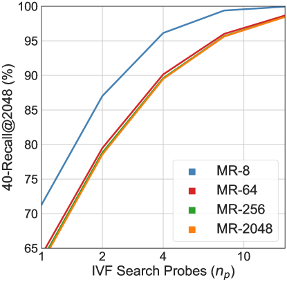
where correct_pred$@k$ is the number of k-NN with correctly predicted labels for a given query. As noted in Section 3, k-Recall@N is the overlap between $k$ exact search nearest neighbors (considered as ground truth) and the top N retrieved documents. As Faiss [24] supports a maximum of 2048-NN while searching the indexed database, we report 40-Recall@2048 in Figure 13. Also note that for ImageNet-1K, which constitutes a bulk of the experimentation in this work, $|Q|=50000$, $|N_{D}|=1281167$ and num_classes $=1000$. For ImageNetv2 [44], $|Q|=10000$ and num_classes $=1000$, and for ImageNet-4K [31], $|Q|=210100$, $|N_{D}|=4202000$ and num_classes $=4202$. For NQ [32], $|Q|=3610$ and $|N_{D}|=21015324$. As NQ consists of question-answer pairs (instance-level), num_classes = $3610$ for the test set.

(a) Exact Search + OPQ on ImageNet-1K

(b) IVF + OPQ on ImageNet-1K

(c) DiskANN + OPQ on ImageNet-1K

(d) HNSW + OPQ on ImageNet-1K

Figure 6: Top-1 Accuracy of ${\rm AdANNS}$ composite indices with OPQ distance computation compared to ${\rm MR}$ and Rigid baselines models on ImageNet-1K and Natural Questions.

Appendix D ${\rm AdANNS}$-OPQ

In this section, we take a deeper dive into the quantization characteristics of ${\rm MR}$. In this work, we restrict our focus to optimized product quantization (OPQ) [13], which adds a learned space rotation and dimensionality permutation to PQ’s sub-vector quantization to learn more optimal PQ codes. We compare OPQ to vanilla PQ on ImageNet in Table 4, and observe large gains at larger embedding dimensionalities, which agrees with the findings of Jayaram Subramanya et al. [22].

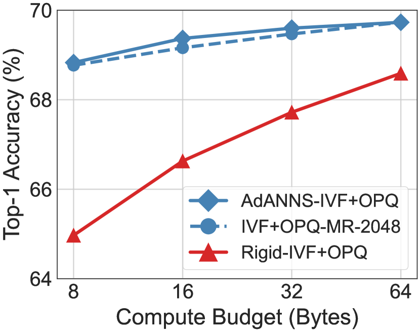
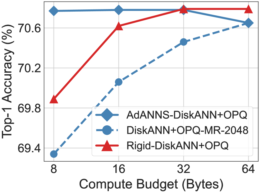
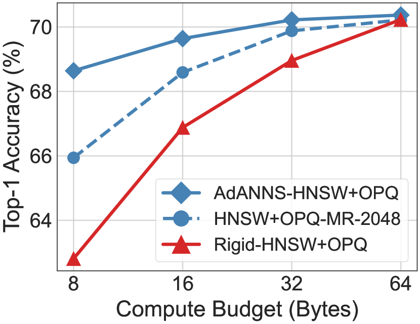
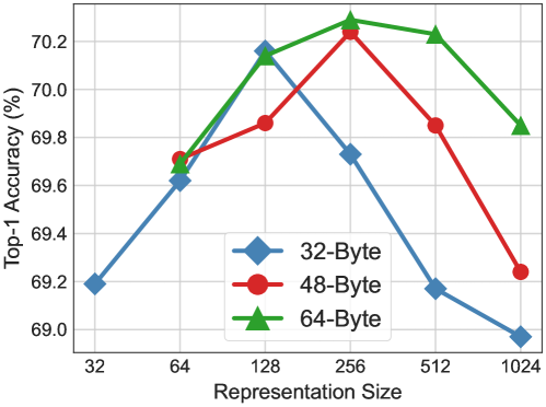
We perform a study of composite OPQ $m\times b$ indices on ImageNet-1K across compression compute budgets $m$ (where $b=8$, i.e. $1$ Byte), i.e. Exact Search with OPQ, IVF+OPQ, HNSW+OPQ, and DiskANN+OPQ, as seen in Figure 6. It is evident from these results:

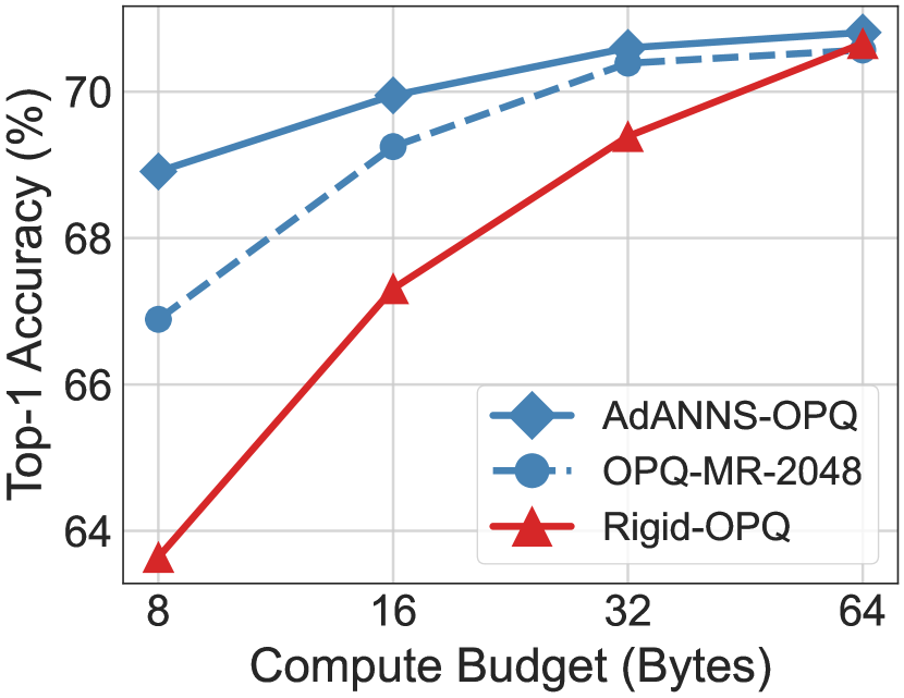
1. Learning OPQ codebooks with ${\rm AdANNS}$ (Figure 6(a)) provides a 1-5% gain in top-1 accuracy over rigid representations at low compute budgets ($\leq 32$ Bytes). ${\rm AdANNS}$-OPQ saturates to Rigid-OPQ performance at low compression ($\geq 64$ Bytes).

2. For IVF, learning clusters with ${\rm MRs}$ instead of ${\rm RRs}$ (Figure 6(b)) provides substantial gains (1-4%). In contrast to Exact-OPQ, using ${\rm AdANNS}$ for learning OPQ codebooks does not provide substantial top-1 accuracy gains over ${\rm MR}$ with $d=2048$ (highest), though it is still slightly better or equal to ${\rm MR}$-2048 at all compute budgets. This further supports that IVF performance generally scales with embedding dimensionality, which is consistent with our findings on ImageNet across robustness variants and encoders (See Figures 9 and 15 respectively).

3. Note that in contrast to Exact, IVF, and HNSW coarse quantizers, DiskANN inherently re-ranks the retrieved shortlist with high-precision embeddings ($d=2048$), which is reflected in its high top-1 accuracy. We find that ${\rm AdANNS}$ with $8$-byte OPQ (Figure 6(c)) matches the top-1 accuracy of rigid representations using $32$-byte OPQ, for a $4\times$ cost reduction for the same accuracy. Also note that using ${\rm AdANNS}$ provides large gains over using ${\rm MR}$-2048 at high compression (1.5%), highlighting the necessity of ${\rm AdANNS}$’s flexibility for high-precision retrieval at low compute budgets.

4. Our findings on the HNSW-OPQ composite index (Figure 6(d)) are consistent with all other indices, i.e. HNSW graphs constructed with ${\rm AdANNS}$ OPQ codebooks provide significant gains over ${\rm RR}$ and ${\rm MR}$, especially at high compression ($\leq 32$ Bytes).

Table 4: Comparison of PQ-${\rm MR}$ with OPQ-${\rm MR}$ for exact search on ImageNet-1K across embedding dimensionality $d\in\{8,16,...,2048\}$ quantized to $m\in\{8,16,32,64\}$ bytes. OPQ shows large gains over vanilla PQ at larger embedding dimensionalities $d\geq 128$. Entries with the highest top-1 accuracy for a given $(d,m)$ tuple are bolded.

Config		PQ			OPQ
d	m	Top-1	mAP@10	P@100	Top-1	mAP@10	P@100
8	8	62.18	56.71	61.23	62.22	56.70	61.23
16	8	67.91	62.85	67.21	67.88	62.96	67.21
	16	67.85	62.95	67.21	67.96	62.94	67.21
32	8	68.80	63.62	67.86	68.91	63.63	67.86
	16	69.57	64.22	68.12	69.47	64.20	68.12
	32	69.44	64.20	68.12	69.47	64.23	68.12
64	8	68.39	63.40	67.47	68.38	63.42	67.60
	16	69.77	64.43	68.25	69.95	64.55	68.38
	32	70.13	64.67	68.38	70.05	64.65	68.38
	64	70.12	64.69	68.42	70.18	64.70	68.38
128	8	67.27	61.99	65.78	68.40	63.11	67.34
	16	69.51	64.32	68.12	69.78	64.56	68.38
	32	70.27	64.72	68.51	70.60	64.97	68.51
	64	70.61	64.93	68.49	70.65	64.98	68.51
256	8	66.06	60.44	64.09	67.90	62.69	66.95
	16	68.56	63.33	66.95	69.92	64.71	68.51
	32	70.08	64.83	68.38	70.59	65.15	68.64
	64	70.48	64.98	68.55	70.69	65.09	68.64
512	8	65.09	59.03	62.53	67.51	62.12	66.56
	16	67.68	62.11	65.39	69.67	64.53	68.38
	32	69.51	64.01	67.34	70.44	65.11	68.64
	64	70.53	65.02	68.52	70.72	65.17	68.64
1024	8	64.58	58.26	61.75	67.26	62.07	66.56
	16	66.84	61.07	64.09	69.34	64.23	68.12
	32	68.71	62.92	66.04	70.43	65.03	68.64
	64	69.88	64.35	67.68	70.81	65.19	68.64
2048	8	62.19	56.11	59.80	66.89	61.69	66.30
	16	65.99	60.27	63.18	69.25	64.09	67.99
	32	67.99	62.04	64.74	70.39	64.97	68.51
	64	69.20	63.46	66.40	70.57	65.15	68.51

OPQ on NQ dataset

(a) Exact Search + OPQ on Natural Questions

(b) IVF + OPQ on Natural Questions

Figure 7: Top-1 Accuracy of ${\rm AdANNS}$ composite indices with OPQ distance computation compared to ${\rm MR}$ and Rigid baselines models on Natural Questions.

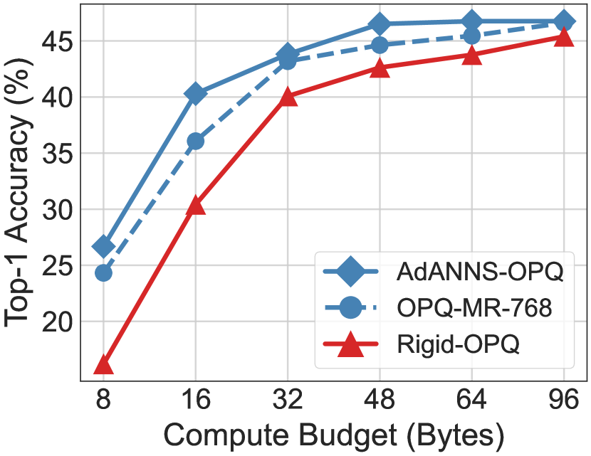
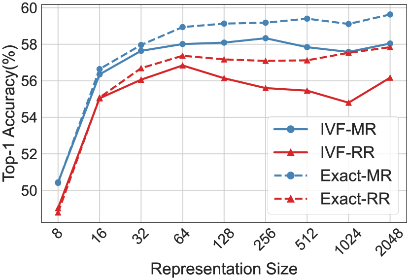
Our observations on ImageNet with ResNet-50 ${\rm MR}$ across search structures also extend to the Natural Questions dataset with Dense Passage Retriever (DPR with BERT-Base ${\rm MR}$ embeddings). We note that ${\rm AdANNS}$ provides gains over ${\rm RR}$-768 embeddings for both Exact Search and IVF with OPQ (Figure 7(a) and 7(b)). We find that similar to ImageNet (Figure 15) IVF performance on Natural Questions generally scales with dimensionality. ${\rm AdANNS}$ thus reduces to ${\rm MR}$-768 performance for $M\geq 16$. See Appendix G for a more in-depth discussion of AdANNS with DPR on Natural Questions.

Appendix E ${\rm AdANNS}$-IVF

Inverted file index (IVF) [48] is a simple yet powerful ANNS data structure used in web-scale search systems [16]. IVF construction involves clustering (coarse quantization often through k-means) [36] on $d$-dimensional representation that results in an inverted file list [53] of all the data points in each cluster. During search, the $d$-dimensional query representation is first assigned to the closest clusters (# probes, typically set to 1) and then an exhaustive linear scan happens within each cluster to obtain the nearest neighbors. As seen in Figure 9, IVF top-1 accuracy scales logarithmically with increasing representation dimensionality $d$ on ImageNet-1K/V2/4K. The learned low-$d$ representations thus provide better accuracy-compute trade-offs compared to high-$d$ representations, thus furthering the case for usage of ${\rm AdANNS}$ with IVF.

Figure 8: Top-1 accuracy vs. compute cost per query of ${\rm AdANNS}$-IVF compared to IVF-${\rm MR}$, IVF-${\rm RR}$ and MG-IVF-${\rm RR}$ baselines on ImageNet-1K.

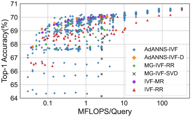
Our proposed adaptive variant of IVF, ${\rm AdANNS}$-IVF, decouples the clustering, with $d_{c}$ dimensions, and the linear scan within each cluster, with $d_{s}$ dimensions – setting $d_{c}=d_{s}$ results in non-adaptive vanilla IVF. This helps in the smooth search of design space for the optimal accuracy-compute trade-off. A naive instantiation yet strong baseline would be to use explicitly trained $d_{c}$ and $d_{s}$ dimensional rigid representations (called MG-IVF-${\rm RR}$, for multi-granular IVF with rigid representations). We also examine the setting of adaptively choosing low-dimensional ${\rm MR}$ to linear scan the shortlisted clusters built with high-dimensional ${\rm MR}$, i.e. ${\rm AdANNS}$-IVF-D, as seen in Table 5. As seen in Figure 8, ${\rm AdANNS}$-IVF provides pareto-optimal accuracy-compute tradeoff across inference compute. This figure is a more exhaustive indication of ${\rm AdANNS}$-IVF behavior compared to baselines than Figures 1(a) and 2. ${\rm AdANNS}$-IVF is evaluated for all possible tuples of $d_{c},d_{s},k=|C|\in\{8,16,\dots,2048\}$. ${\rm AdANNS}$-IVF-D is evaluated for a pre-built IVF index with $d_{c}=2048$ and $d_{s}\in\{8,\dots,2048\}$. MG-IVF-${\rm RR}$ configurations are evaluated for $d_{c}\in\{8,\dots,d_{s}\}$, $d_{s}\in\{32,\dots,2048\}$ and $k=1024$ clusters. A study over additional $k$ values is omitted due to high compute cost. Finally, IVF-${\rm MR}$ and IVF-${\rm RR}$ configurations are evaluated for $d_{c}=d_{s}\in\{8,16,\dots,2048\}$ and $k\in\{256,\dots,8192\}$. Note that for a fair comparison, we use $n_{p}=1$ across all configurations. We discuss the inference compute for these settings in Appendix B.1.

E.1 Robustness

(a) ImageNet-1K

(b) ImageNetV2

(c) ImageNet-4K

Figure 9: Top-1 Accuracy variation of IVF-${\rm MR}$ of ImageNet 1K, ImageNetV2 and ImageNet-4K. ${\rm RR}$ baselines are omitted on ImageNet-4K due to high compute cost.

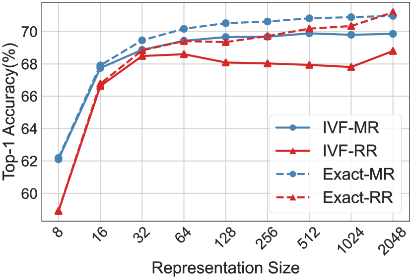
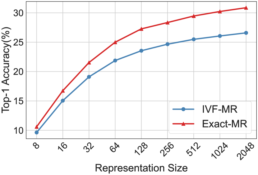
As shown in Figure 9, we examined the clustering capabilities of ${\rm MRs}$ on both in-distribution (ID) queries via ImageNet-1K and out-of-distribution (OOD) queries via ImageNetV2 [44], as well as on larger-scale ImageNet-4K [31]. For ID queries on ImageNet-1K (Figure 9(a)), IVF-${\rm MR}$ is at least as accurate as Exact-${\rm RR}$ for $d\leq 256$ with a single search probe, demonstrating the quality of in-distribution low-d clustering with ${\rm MR}$. On OOD queries (Figure 9(b)), we observe that IVF-${\rm MR}$ is on average $2\%$ more robust than IVF-${\rm RR}$ across all cluster construction and linear scan dimensionalities $d$. It is also notable that clustering with ${\rm MRs}$ followed by linear scan with # probes $=1$ is more robust than exact search with ${\rm RR}$ embeddings across all $d\leq 2048$, indicating the adaptability of ${\rm MRs}$ to distribution shifts during inference. As seen in Table 5, on ImageNetV2 ${\rm AdANNS}$-IVF-D is the best configuration for $d\leq 16$, and is similarly accurate to IVF-${\rm MR}$ at all other $d$. ${\rm AdANNS}$-IVF-D with $d=128$ is able to match its own accuracy with $d=2048$, a $16\times$ compute gain during inference. This demonstrates the potential of ${\rm AdANNS}$ to adaptively search pre-indexed clustering structures.

On 4-million scale ImageNet-4K (Figure 9(c)), we observe similar accuracy trends of IVF-${\rm MR}$ compared to Exact-${\rm MR}$ as in ImageNet-1K (Figure 9(a)) and ImageNetV2 (Figure 9(b)). We omit baseline IVF-${\rm RR}$ and Exact-${\rm RR}$ experiments due to high compute cost at larger scale.

Table 5: Top-1 Accuracy of ${\rm AdANNS}$-IVF-D on out-of-distribution queries from ImageNetV2 compared to both IVF and Exact Search with ${\rm MR}$ and ${\rm RR}$ embeddings. Note that for ${\rm AdANNS}$-IVF-D, the dimensionality used to build clusters $d_{c}=2048$.

d	${\rm AdANNS}$-IVF-D	IVF-${\rm MR}$	Exact-${\rm MR}$	IVF-${\rm RR}$	Exact-${\rm RR}$
8	53.51	50.44	50.41	49.03	48.79
16	57.32	56.35	56.64	55.04	55.08
32	57.32	57.64	57.96	56.06	56.69
64	57.85	58.01	58.94	56.84	57.37
128	58.02	58.09	59.13	56.14	57.17
256	58.01	58.33	59.18	55.60	57.09
512	58.03	57.84	59.40	55.46	57.12
1024	57.66	57.58	59.11	54.80	57.53
2048	58.04	58.04	59.63	56.17	57.84

E.2 IVF-${\rm MR}$ Ablations

(a) 4K Search Probes ($n_{p}$)

(b) Centroid Recall

Figure 10: Ablations on IVF-${\rm MR}$ Clustering: a) Analysis of accuracy-compute tradeoff with increasing IVF-${\rm MR}$ search probes $n_{p}$ on ImageNet-4K compared to Exact-${\rm MR}$ and b) k-Recall@N on ImageNet-1K cluster centroids across representation sizes $d$. Cluster centroids retrieved with highest embedding dim $d=2048$ were considered ground-truth centroids.

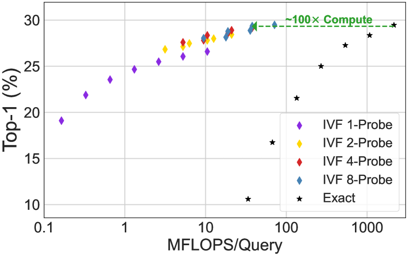
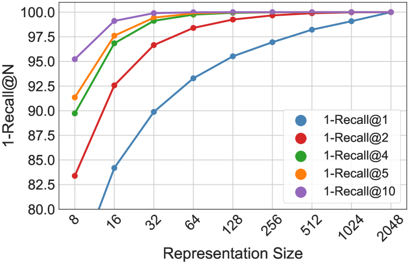
As seen in Figure 10(a), IVF-${\rm MR}$ can match the accuracy of Exact Search on ImageNet-4K with $\sim 100\times$ less compute. We also explored the capability of ${\rm MRs}$ at retrieving cluster centroids with low-d compared to a ground truth of 2048-d with k-Recall@N, as seen in Figure 10(b). ${\rm MRs}$ were able to saturate to near-perfect 1-Recall@N for $d\geq 32$ and $N\geq 4$, indicating the potential of ${\rm AdANNS}$ at matching exact search performance with less than 10 search probes $n_{p}$.

Figure 11: Clustering distributions for IVF-${\rm MR}$ and IVF-${\rm RR}$ across embedding dimensionality $d$ on ImageNet-1K. An IVF-${\rm MR}$ and IVF-${\rm RR}$ clustered with $d=16$ embeddings is denoted by ${\rm MR}$-$16$ and ${\rm RR}$-$16$ respectively.

E.3 Clustering Distribution

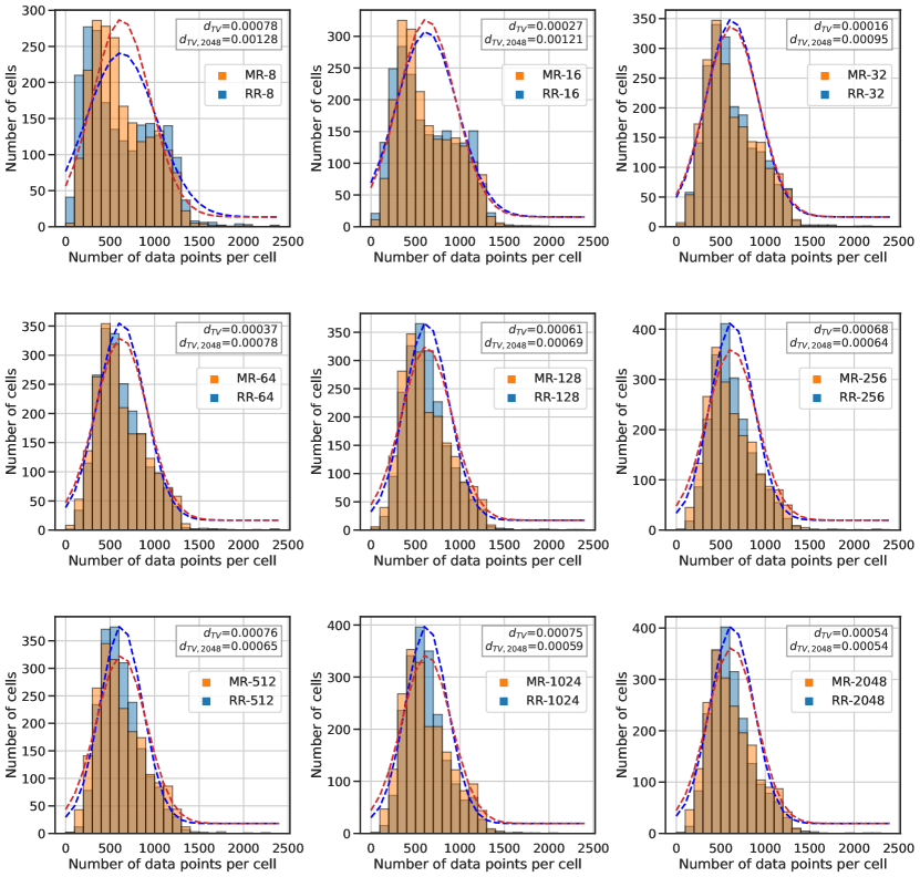
We examined the distribution of learnt clusters across embedding dimensionalities $d$ for both ${\rm MR}$ and ${\rm RR}$ models, as seen in Figure 11. We observe IVF-${\rm MR}$ to have less variance than IVF-${\rm RR}$ at $d\in\{8,16\}$, and slightly higher variance for $d\geq 32$, while IVF-${\rm MR}$ outperforms IVF-${\rm RR}$ in top-1 across all $d$ (Figure 9(a)). This indicates that although ${\rm MR}$ learns clusters that are less uniformly distributed than ${\rm RR}$ at high $d$, the quality of learnt clustering is superior to ${\rm RR}$ across all $d$. Note that a uniform distribution is $N/k$ data points per cluster, i.e. $\sim 1250$ for ImageNet-1K with $k=1024$. We quantitatively evaluate the proximity of the ${\rm MR}$ and ${\rm RR}$ clustering distributions with Total Variation Distance [33], which is defined over two discrete probability distributions $p,q$ over $[n]$ as follows:

$$d_{TV}(p,q)=\dfrac{1}{2}\sum\limits_{i\in[n]}|p_{i}-q_{i}|$$

We also compute $d_{TV,2048}({\rm MR}\text{-d})=d_{TV}({\rm MR}\text{-d},{\rm RR}\text{-2048})$, which evaluates the total variation distance of a given low-d ${\rm MR}$ from high-d ${\rm RR}$-2048. We observe a monotonically decreasing $d_{TV,2048}$ with increasing $d$, which demonstrates that ${\rm MR}$ clustering distributions get closer to ${\rm RR}$-2048 as we increase the embedding dimensionality $d$. We observe in Figure 11 that $d_{TV}({\rm MR}\text{-d},{\rm RR}\text{-d})\sim 7e-4$ for $d\in\{8,256,\dots,2048\}$ and $\sim 3e-4$ for $d\in\{16,32,64\}$. These findings agree with the top-1 improvement of ${\rm MR}$ over ${\rm RR}$ as shown in Figure 9(a), where there are smaller improvements for $d\in\{16,32,64\}$ (smaller $d_{TV}$) and larger improvements for $d\in\{8,256,\dots,2048\}$ (larger $d_{TV}$). These results demonstrate a correlation between top-1 performance of IVF-${\rm MR}$ and the quality of clusters learnt with ${\rm MR}$.

Appendix F ${\rm AdANNS}$-DiskANN

Table 6: Wall clock search latency ($\mu{s}$) of ${\rm AdANNS}$-DiskANN across graph construction dimensionality $d\in\{8,16,\dots,2048\}$ and compute budget in terms of OPQ budget $M\in\{8,16,32,48,64\}$. Search latency is fairly consistent across fixed embedding dimensionality $D$.

$d$	$M$=8	$M$=16	$M$=32	$M$=48	$M$=64
8	495	-	-	-	-
16	555	571	-	-	-
32	669	655	653	-	-
64	864	855	843	844	848
128	1182	1311	1156	1161	2011
256	1923	1779	1744	2849	1818
512	2802	3272	3423	2780	3171
1024	5127	5456	5724	4683	5087
2048	9907	9833	10205	10183	9329

DiskANN is a state-of-the-art graph-based ANNS index capable of serving queries from both RAM and SSD. DiskANN builds a greedy best-first graph with OPQ distance computation, with compressed vectors stored in memory. The index and full-precision vectors are stored on the SSD. During search, when a query’s neighbor shortlist is fetched from the SSD, its full-precision vector is also fetched in a single disk read. This enables efficient and fast distance computation with PQ on a large initial shortlist of candidate nearest neighbors in RAM followed by a high-precision re-ranking with full-precision vectors fetched from the SSD on a much smaller shortlist. The experiments carried out in this work primarily utilize a DiskANN graph index built in-memory with OPQ distance computation.

Figure 12: DiskANN-${\rm MR}$ with SSD indices for ImageNet-1K retrieval, with compute budgets $m_{disk}=m_{dc}\in\{32,48,64\}$ across graph and OPQ codebook construction dimensionalities $d\in\{32,\dots,1024\}$. Note that this does not use any re-ranking after obtaining OPQ based shortlist.

As with IVF, DiskANN is also well suited to the flexibility provided by ${\rm AdANNS}$ as we demonstrate on both ImageNet and NQ that the optimal PQ codebook for a given compute budget is learnt with a smaller embedding dimensionality $d$ (see Figures 6(c) and  7(a)). We demonstrate the capability of ${\rm AdANNS}$-DiskANN with a compute budget of $m\in\{32,64\}$ in Table 4.3. We tabulate the search time latency of ${\rm AdANNS}$-DiskANN in microseconds ($\mu{s}$) in Table 6, which grows linearly with graph construction dimensionality $d$. We also examine DiskANN-${\rm MR}$ with SSD graph indices on ImageNet-1K across OPQ budgets for distance computation $m_{dc}\in\{32,48,64\}$, as seen in Figure 12. With SSD indices, we store PQ-compressed vectors on disk with $m_{disk}=m_{dc}$, which essentially disables DiskANN’s implicit high-precision re-ranking. We observe similar trends to other composite ANNS indices on ImageNet, where the optimal dim for fixed OPQ budget is not the highest dim ($d=1024$ with fp32 embeddings is current highest dim supported by DiskANN which stores vectors in 4KB sectors on disk). This provides further motivation for ${\rm AdANNS}$-DiskANN, which leverages ${\rm MRs}$ to provide flexible access to the optimal dim for quantization and thus enables similar Top-1 accuracy to Rigid DiskANN for up to $1/4$ the cost (Figure 6(c)).

Appendix G ${\rm AdANNS}$ on Natural Questions

In addition to image retrieval on ImageNet, we also experiment with dense passage retrieval (DPR) on Natural Questions. As shown in Figure 6, ${\rm MR}$ representations are $1-10\%$ more accurate than their ${\rm RR}$ counterparts across PQ compute budgets with Exact Search + OPQ on NQ. We also demonstrate that IVF-${\rm MR}$ is $1-2.5\%$ better than IVF-${\rm RR}$ for Precision@$k$, $k\in\{1,5,20,100,200\}$. Note that on NQ, IVF loses $\sim 10\%$ accuracy compared to exact search, even with the ${\rm RR}$-768 baseline. We hypothesize the weak performance of IVF owing to poor clusterability of the BERT-Base embeddings fine-tuned on the NQ dataset. A more thorough exploration of ${\rm AdANNS}$-IVF on NQ is an immediate future work and is in progress.

Appendix H Ablations

H.1 Recall Score Analysis

Figure 13: k-Recall@N of $d$-dimensional ${\rm MR}$ for IVF and HNSW with increasing search probes $n_{p}$ on ImageNet-1K and ImageNet-4K. On ImageNet-4K, we restrict our study to IVF-${\rm MR}$ with $d\in\{8,64,256,2048\}$. Other embedding dimensionalities, HNSW-${\rm MR}$ and ${\rm RR}$ baselines are omitted due to high compute cost. We observe that trends from ImageNet-1K with increasing $d$ and $n_{p}$ extend to ImageNet-4K, which is $4\times$ larger.

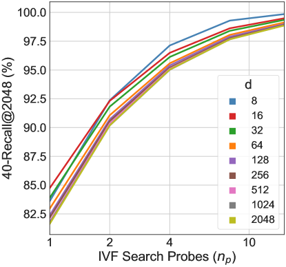
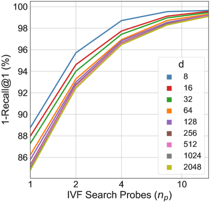
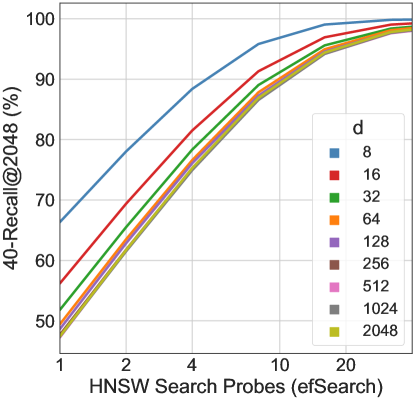
In this section we also examine the variation of k-Recall@N with by probing a larger search space with IVF and HNSW indices. For IVF, search probes represent the number of clusters shortlisted for linear scan during inference. For HNSW, search quality is controlled by the $efSearch$ parameter [38], which represents the closest neighbors to query $q$ at level $l_{c}$ of the graph and is analogous to number of search probes in IVF. As seen in Figure 13, general trends show a) an intuitive increase in recall with increasing search probes $n_{p}$) for fixed search probes, b) a decrease in recall with increasing search dimensionality $d$ c) similar trends in ImageNet-1K and $4\times$ larger ImageNet-4K.

H.2 Relative Contrast

Figure 14: Relative contrast of varying capacity ${\rm MRs}$ and ${\rm RRs}$ on ImageNet-1K corroborating the findings of He et al. [18].

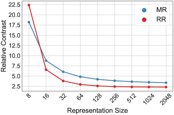
We utilize Relative Contrast [18] to capture the difficulty of nearest neighbors search with IVF-${\rm MR}$ compared to IVF-${\rm RR}$. For a given database $X=\{x_{i}\in\mathbb{R}^{d},i=1,\dots,N_{D}\}$, a query $q\in\mathbb{R}^{d}$, and a distance metric $D(.,.)$ we compute relative contrast $C_{r}$ as a measure of the difficulty in finding the 1-nearest neighbor (1-NN) for a query $q$ in database $X$ as follows:

1. Compute $D_{min}^{q}=\min\limits_{i=1...n}D(q,x_{i})$, i.e. the distance of query $q$ to its nearest neighbor $x_{nn}^{q}\in X$

2. Compute $D_{mean}^{q}=E_{x}[D(q,x)]$ as the average distance of query $q$ from all database points $x\in X$

3. Relative Contrast of a given query $C_{r}^{q}=\dfrac{D_{mean}^{q}}{D_{min}^{q}}$, which is a measure of how separable the query’s nearest neighbor $x_{nn}^{q}$ is from an average point in the database $x$

4. Compute an expectation over all queries for Relative Contrast over the entire database as

   $$C_{r}=\dfrac{E_{q}[D_{mean}^{q}]}{E_{q}[D_{min}^{q}]}$$

It is evident that $C_{r}$ captures the difficulty of Nearest Neighbor Search in database $X$, as a $C_{r}\sim 1$ indicates that for an average query, its nearest neighbor is almost equidistant from a random point in the database. As demonstrated in Figure 14, ${\rm MRs}$ have higher $R_{c}$ than ${\rm RR}$ Embeddings for an Exact Search on ImageNet-1K for all $d\geq 16$. This result implies that a portion of ${\rm MR}$’s improvement over ${\rm RR}$ for 1-NN retrieval across all embedding dimensionalities $d$ [31] is due to a higher average separability of the ${\rm MR}$ 1-NN from a random database point.

H.3 Generality across Encoders

We perform an ablation over the representation function $\phi:X\to\mathbb{R}^{d}$ learnt via a backbone neural network (primarily ResNet50 in this work), as detailed in Section 3. We also train MRL models [31] $\phi^{MR(d)}$ on ResNet18/34/101 [19] that are as accurate as their independently trained ${\rm RR}$ baseline models $\phi^{RR(d)}$, where $d$ is the default max representation size of each architecture. We also train MRL with a ConvNeXt-Tiny backbone with $[d]=\{48,96,192,384,786\}$. ${\rm MR}$-$768$ has a top-1 accuracy of $79.45\%$ compared to independently trained publicly available ${\rm RR}$-$768$ baseline with top-1 accuracy $82.1\%$ (Code and ${\rm RR}$ model available on the official repo). We note that this training had no hyperparameter tuning whatsoever, and this gap can be closed with additional model training effort. We then compare clustering the ${\rm MRs}$ via IVF-${\rm MR}$ with $k=2048,n_{p}=1$ on ImageNet-1K to Exact-${\rm MR}$, which is shown in Figure 15. IVF-${\rm MR}$ shows similar trends across backbones compared to Exact-${\rm MR}$, i.e. a maximum top-1 accuracy drop of $\sim 1.6\%$ for a single search probe. This suggests the clustering capabilities of ${\rm MR}$ extend beyond an inductive bias of $\phi^{MR(d)}\in$ ResNet50, though we leave a detailed exploration for future work.

Figure 15: Top-1 Accuracy variation of IVF-${\rm MR}$ on ImageNet-1K with different embedding representation function $\phi^{MR(d)}$ (see Section 3), where $\phi\in$ {ResNet18/34/101, ConvNeXt-Tiny}. We observe similar trends between IVF-${\rm MR}$ and Exact-${\rm MR}$ on ResNet18/34/101 when compared to ResNet50 (Figure 9(a)) which is the default in all experiments in this work.

References

- Aumüller et al. [2020] M. Aumüller, E. Bernhardsson, and A. Faithfull. Ann-benchmarks: A benchmarking tool for approximate nearest neighbor algorithms. Information Systems, 87:101374, 2020.
- Bengio [2012] Y. Bengio. Deep learning of representations for unsupervised and transfer learning. In Proceedings of ICML workshop on unsupervised and transfer learning, pages 17–36. JMLR Workshop and Conference Proceedings, 2012.
- Bernhardsson [2018] E. Bernhardsson. Annoy: Approximate Nearest Neighbors in C++/Python, 2018. URL https://pypi.org/project/annoy/. Python package version 1.13.0.
- Brin and Page [1998] S. Brin and L. Page. The anatomy of a large-scale hypertextual web search engine. Computer networks and ISDN systems, 30(1-7):107–117, 1998.
- Cai [2021] D. Cai. A revisit of hashing algorithms for approximate nearest neighbor search. IEEE Transactions on Knowledge and Data Engineering, 33(6):2337–2348, 2021. doi: 10.1109/TKDE.2019.2953897.
- Chen et al. [2020] T. Chen, L. Li, and Y. Sun. Differentiable product quantization for end-to-end embedding compression. In International Conference on Machine Learning, pages 1617–1626. PMLR, 2020.
- Clarkson [1994] K. L. Clarkson. An algorithm for approximate closest-point queries. In Proceedings of the tenth annual symposium on Computational geometry, pages 160–164, 1994.
- Datar et al. [2004] M. Datar, N. Immorlica, P. Indyk, and V. S. Mirrokni. Locality-sensitive hashing scheme based on p-stable distributions. In Proceedings of the twentieth annual symposium on Computational geometry, pages 253–262, 2004.
- Dean [2009] J. Dean. Challenges in building large-scale information retrieval systems. In Keynote of the 2nd ACM International Conference on Web Search and Data Mining (WSDM), volume 10, 2009.
- Devlin et al. [2018] J. Devlin, M.-W. Chang, K. Lee, and K. Toutanova. Bert: Pre-training of deep bidirectional transformers for language understanding. arXiv preprint arXiv:1810.04805, 2018.
- Devvrit et al. [2023] Devvrit, S. Kudugunta, A. Kusupati, T. Dettmers, K. Chen, I. Dhillon, Y. Tsvetkov, H. Hannaneh, S. Kakade, A. Farhadi, and P. Jain. Matformer: Nested transformer for elastic inference. arXiv preprint arxiv:2310.07707, 2023.
- Friedman et al. [1977] J. H. Friedman, J. L. Bentley, and R. A. Finkel. An algorithm for finding best matches in logarithmic expected time. ACM Transactions on Mathematical Software (TOMS), 3(3):209–226, 1977.
- Ge et al. [2013] T. Ge, K. He, Q. Ke, and J. Sun. Optimized product quantization for approximate nearest neighbor search. In Proceedings of the IEEE Conference on Computer Vision and Pattern Recognition, pages 2946–2953, 2013.
- Golub and Kahan [1965] G. Golub and W. Kahan. Calculating the singular values and pseudo-inverse of a matrix. Journal of the Society for Industrial and Applied Mathematics, Series B: Numerical Analysis, 2(2):205–224, 1965.
- Gray [1984] R. Gray. Vector quantization. IEEE Assp Magazine, 1(2):4–29, 1984.
- Guo et al. [2020] R. Guo, P. Sun, E. Lindgren, Q. Geng, D. Simcha, F. Chern, and S. Kumar. Accelerating large-scale inference with anisotropic vector quantization. In International Conference on Machine Learning, pages 3887–3896. PMLR, 2020.
- Gupta et al. [2022] N. Gupta, P. H. Chen, H.-F. Yu, C.-J. Hsieh, and I. S. Dhillon. End-to-end learning to index and search in large output spaces. arXiv preprint arXiv:2210.08410, 2022.
- He et al. [2012] J. He, S. Kumar, and S.-F. Chang. On the difficulty of nearest neighbor search. In International Conference on Machine Learning (ICML), 2012.
- He et al. [2016] K. He, X. Zhang, S. Ren, and J. Sun. Deep residual learning for image recognition. In Proceedings of the IEEE conference on computer vision and pattern recognition, pages 770–778, 2016.
- He et al. [2020] K. He, H. Fan, Y. Wu, S. Xie, and R. Girshick. Momentum contrast for unsupervised visual representation learning. In Proceedings of the IEEE/CVF conference on computer vision and pattern recognition, pages 9729–9738, 2020.
- Indyk and Motwani [1998] P. Indyk and R. Motwani. Approximate nearest neighbors: towards removing the curse of dimensionality. In Proceedings of the thirtieth annual ACM symposium on Theory of computing, pages 604–613, 1998.
- Jayaram Subramanya et al. [2019] S. Jayaram Subramanya, F. Devvrit, H. V. Simhadri, R. Krishnawamy, and R. Kadekodi. Diskann: Fast accurate billion-point nearest neighbor search on a single node. Advances in Neural Information Processing Systems, 32, 2019.
- Jegou et al. [2010] H. Jegou, M. Douze, and C. Schmid. Product quantization for nearest neighbor search. IEEE transactions on pattern analysis and machine intelligence, 33(1):117–128, 2010.
- Johnson et al. [2019] J. Johnson, M. Douze, and H. Jégou. Billion-scale similarity search with GPUs. IEEE Transactions on Big Data, 7(3):535–547, 2019.
- Johnson [1984] W. B. Johnson. Extensions of lipschitz mappings into a hilbert space. Contemp. Math., 26:189–206, 1984.
- Jolliffe and Cadima [2016] I. T. Jolliffe and J. Cadima. Principal component analysis: a review and recent developments. Philosophical Transactions of the Royal Society A: Mathematical, Physical and Engineering Sciences, 374(2065):20150202, 2016.
- Karpukhin et al. [2020] V. Karpukhin, B. Oğuz, S. Min, P. Lewis, L. Wu, S. Edunov, D. Chen, and W.-t. Yih. Dense passage retrieval for open-domain question answering. arXiv preprint arXiv:2004.04906, 2020.
- Kornblith et al. [2019] S. Kornblith, J. Shlens, and Q. V. Le. Do better imagenet models transfer better? In Proceedings of the IEEE/CVF conference on computer vision and pattern recognition, pages 2661–2671, 2019.
- Kraska et al. [2018] T. Kraska, A. Beutel, E. H. Chi, J. Dean, and N. Polyzotis. The case for learned index structures. In Proceedings of the 2018 international conference on management of data, pages 489–504, 2018.
- Kusupati et al. [2021] A. Kusupati, M. Wallingford, V. Ramanujan, R. Somani, J. S. Park, K. Pillutla, P. Jain, S. Kakade, and A. Farhadi. Llc: Accurate, multi-purpose learnt low-dimensional binary codes. Advances in Neural Information Processing Systems, 34:23900–23913, 2021.
- Kusupati et al. [2022] A. Kusupati, G. Bhatt, A. Rege, M. Wallingford, A. Sinha, V. Ramanujan, W. Howard-Snyder, K. Chen, S. Kakade, P. Jain, and A. Farhadi. Matryoshka representation learning. In Advances in Neural Information Processing Systems, December 2022.
- Kwiatkowski et al. [2019] T. Kwiatkowski, J. Palomaki, O. Redfield, M. Collins, A. Parikh, C. Alberti, D. Epstein, I. Polosukhin, J. Devlin, K. Lee, et al. Natural questions: a benchmark for question answering research. Transactions of the Association for Computational Linguistics, 7:453–466, 2019.
- Levin and Peres [2017] D. A. Levin and Y. Peres. Markov chains and mixing times, volume 107. American Mathematical Soc., 2017.
- Li et al. [2020] W. Li, Y. Zhang, Y. Sun, W. Wang, W. Zhang, and X. Lin. Approximate nearest neighbor search on high dimensional data—experiments, analyses, and improvement. IEEE Transactions on Knowledge and Data Engineering, 2020.
- Liu et al. [2022] Z. Liu, H. Mao, C.-Y. Wu, C. Feichtenhofer, T. Darrell, and S. Xie. A convnet for the 2020s. In Proceedings of the IEEE/CVF Conference on Computer Vision and Pattern Recognition, pages 11976–11986, 2022.
- Lloyd [1982] S. Lloyd. Least squares quantization in pcm. IEEE transactions on information theory, 28(2):129–137, 1982.
- Malkov et al. [2014] Y. Malkov, A. Ponomarenko, A. Logvinov, and V. Krylov. Approximate nearest neighbor algorithm based on navigable small world graphs. Information Systems, 45:61–68, 2014.
- Malkov and Yashunin [2020] Y. A. Malkov and D. Yashunin. Efficient and robust approximate nearest neighbor search using hierarchical navigable small world graphs. IEEE Transactions on Pattern Analysis & Machine Intelligence, 42(04):824–836, 2020.
- Mardia et al. [1979] K. Mardia, J. Kent, and J. Bibby. Multivariate analysis. Probability and Mathematical Statistics, 1979.
- Nayak [2019] P. Nayak. Understanding searches better than ever before. Google AI Blog, 2019. URL https://blog.google/products/search/search-language-understanding-bert/.
- Neelakantan et al. [2022] A. Neelakantan, T. Xu, R. Puri, A. Radford, J. M. Han, J. Tworek, Q. Yuan, N. Tezak, J. W. Kim, C. Hallacy, et al. Text and code embeddings by contrastive pre-training. arXiv preprint arXiv:2201.10005, 2022.
- Radford et al. [2021] A. Radford, J. W. Kim, C. Hallacy, A. Ramesh, G. Goh, S. Agarwal, G. Sastry, A. Askell, P. Mishkin, J. Clark, et al. Learning transferable visual models from natural language supervision. In International Conference on Machine Learning, pages 8748–8763. PMLR, 2021.
- Ramanujan et al. [2021] V. Ramanujan, P. K. A. Vasu, A. Farhadi, O. Tuzel, and H. Pouransari. Forward compatible training for representation learning. arXiv preprint arXiv:2112.02805, 2021.
- Recht et al. [2019] B. Recht, R. Roelofs, L. Schmidt, and V. Shankar. Do imagenet classifiers generalize to imagenet? In International Conference on Machine Learning, pages 5389–5400. PMLR, 2019.
- Russakovsky et al. [2015] O. Russakovsky, J. Deng, H. Su, J. Krause, S. Satheesh, S. Ma, Z. Huang, A. Karpathy, A. Khosla, M. Bernstein, et al. Imagenet large scale visual recognition challenge. International journal of computer vision, 115(3):211–252, 2015.
- Salakhutdinov and Hinton [2009] R. Salakhutdinov and G. Hinton. Semantic hashing. International Journal of Approximate Reasoning, 50(7):969–978, 2009.
- Simhadri et al. [2022] H. V. Simhadri, G. Williams, M. Aumüller, M. Douze, A. Babenko, D. Baranchuk, Q. Chen, L. Hosseini, R. Krishnaswamy, G. Srinivasa, et al. Results of the neurips’21 challenge on billion-scale approximate nearest neighbor search. arXiv preprint arXiv:2205.03763, 2022.
- Sivic and Zisserman [2003] J. Sivic and A. Zisserman. Video google: A text retrieval approach to object matching in videos. In Computer Vision, IEEE International Conference on, volume 3, pages 1470–1470. IEEE Computer Society, 2003.
- Soudry et al. [2018] D. Soudry, E. Hoffer, M. S. Nacson, S. Gunasekar, and N. Srebro. The implicit bias of gradient descent on separable data. The Journal of Machine Learning Research, 19(1):2822–2878, 2018.
- Waldburger [2019] C. Waldburger. As search needs evolve, microsoft makes ai tools for better search available to researchers and developers. Microsoft AI Blog, 2019. URL https://blogs.microsoft.com/ai/bing-vector-search/.
- Wang et al. [2021] M. Wang, X. Xu, Q. Yue, and Y. Wang. A comprehensive survey and experimental comparison of graph-based approximate nearest neighbor search. Proceedings of the VLDB Endowment, 14(11):1964–1978, 2021.
- Weber et al. [1998] R. Weber, H.-J. Schek, and S. Blott. A quantitative analysis and performance study for similarity-search methods in high-dimensional spaces. In VLDB, volume 98, pages 194–205, 1998.
- Witten et al. [1999] I. H. Witten, I. H. Witten, A. Moffat, T. C. Bell, T. C. Bell, E. Fox, and T. C. Bell. Managing gigabytes: compressing and indexing documents and images. Morgan Kaufmann, 1999.
Appendix A Framework