CSP: Self-Supervised Contrastive Spatial Pre-Training
for Geospatial-Visual Representations

Abstract

Geo-tagged images are publicly available in large quantities, whereas labels such as object classes are rather scarce and expensive to collect. Meanwhile, contrastive learning has achieved tremendous success in various natural image and language tasks with limited labeled data. However, existing methods fail to fully leverage geospatial information, which can be paramount to distinguishing objects that are visually similar. To directly leverage the abundant geospatial information associated with images in pre-training, fine-tuning, and inference stages, we present Contrastive Spatial Pre-Training (CSP), a self-supervised learning framework for geo-tagged images. We use a dual-encoder to separately encode the images and their corresponding geo-locations, and use contrastive objectives to learn effective location representations from images, which can be transferred to downstream supervised tasks such as image classification. Experiments show that CSP can improve model performance on both iNat2018 and fMoW dataset. Especially, on iNat2018, CSP significantly boosts the model performance with 10-34% relative improvement with various labeled training data sampling ratios.

1 Introduction

(a) Arctic Fox

(b) Arctic Fox Locations

(c) Bat-Eared Fox

(d) Bat-Eared Fox Locations

Figure 1: The importance of geospatial information demonstrated by two visually similar species (a)(c), and their distinct patterns in image locations (b)(d).

(a) Sup. Only: Geo-aware Supervised Learning (Mac Aodha et al., 2019; Mai et al., 2020b)

(b) Img. Only: Image Encoder Pre-Training with Geographic Knowledge (Jean et al., 2019; Ayush et al., 2021; Manas et al., 2021; Li et al., 2021a). Here we show four previous approaches to pre-train the image encoder $f()$ (orange box). A detailed version can be seen in Figure 6 in Appendix A.1.

(c) Contrastive Spatial Pre-Training  (CSP). It adds a location encoder pre-training stage (red box). The pre-trained $f()$ is used as an unsupervised feature extractor to generate image embeddings $f(\mathbf{I})$ which are used for contrastive learning with location embedding $e(\bm{\mathbf{x}})$. Both $f()$ and $e()$ are fine-tuned in a supervised manner (green and blue box).

Figure 2: Different training strategies for geo-aware image classification. Our proposed method CSP is presented in Figure 2(c).

Low-data or few-shot regimes (Zhai et al., 2021; Wang et al., 2020) is a prevalent challenge in the geospatial domain, where we usually have access to massive amounts of unlabeled data while only limited amount of labeled data is available. For example, users on Flickr, Google Photos, and iNaturalist App upload millions of geo-tagged images every day, and multiple satellites continuously capture remote sensing (RS) images with corresponding geo-coordinates all over the world. These geo-tagged data form large publicly available unlabeled datasets that are inexpensive to obtain. In contrast, desired labels for many geospatial tasks (e.g., object class labels, object bounding boxes, and land use type labels, etc.) are rather scarce and expensive to collect. Moreover, even well-curated and widely used labeled geospatial datasets such as UC Merced Land Use Dataset (Yang & Newsam, 2010) and BigEarthNet (Sumbul et al., 2019) have limited sizes, geographic coverage, and potentially oversimplified label distributions. This lack of labeled data coverage severely limits the ability to generalize, especially in a geographic sense, of models trained on these labeled geospatial datasets (Goodchild & Li, 2021).

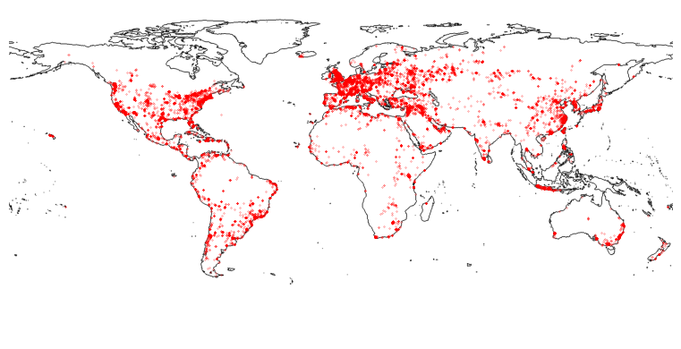
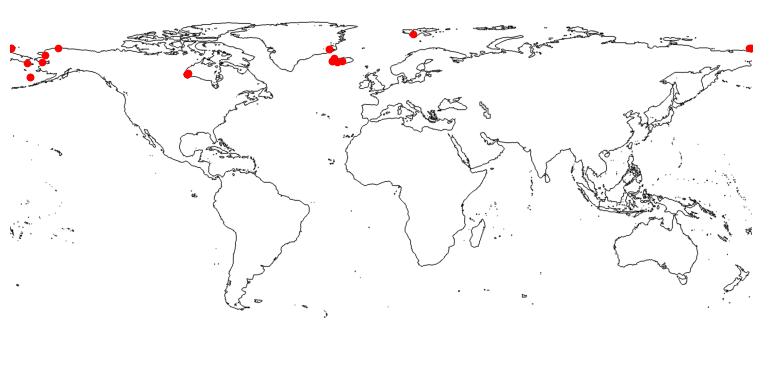
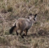
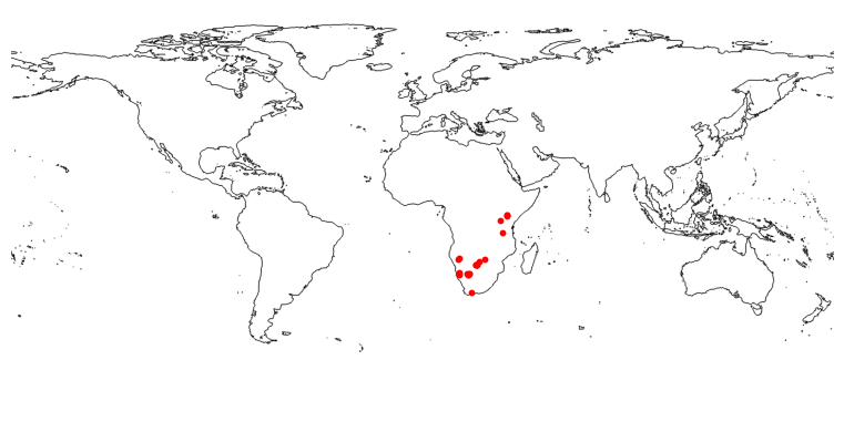
Meanwhile, numerous previous studies have shown the great potential of leveraging geospatial information as complementary information for visual cues to help improve the model performance on various computer vision tasks (Tang et al., 2015; Chu et al., 2019; Mac Aodha et al., 2019; Klocek et al., 2019; Mai et al., 2020b, 2022d; Yang et al., 2022). For example, Figure 1(a) and 1(c) are images of two different fox species: Arctic fox and bat-eared fox, with which the vision-based models, or even humans, can be confused due to the high visual similarity of the two species and their surrounding environments. Fortunately, these two species have distinct geospatial distribution patterns (shown in Figure 1(b), 1(d)), and it is very easy to tell them apart based on the geo-locations. Motivated by these observations, we ask whether we can build a multi-modal self-supervised learning framework between geo-locations and images that learns the alignments between geo-location and image representations using large unlabeled geo-tagged datasets.

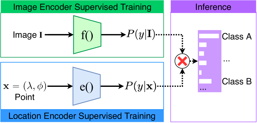
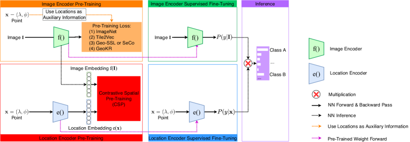
In this work, we propose CSP (Contrastive Spatial Pre-Training), a self-supervised learning framework, which pre-trains deep spatial representations from unlabeled geo-tagged images by predicting image features or image identities based on their geo-locations as shown in Figure 2(c). Given one location-image pair $(\bm{\mathbf{x}}_{i},\mathbf{I}_{i})$, a dual-encoder separately encodes $\bm{\mathbf{x}}_{i}$ and $\mathbf{I}_{i}$ into the embedding space with a location encoder $e()$ and an image encoder $f()$ and contrast against related locations and images to form a contrastive learning objective (the red box in Figure 2(c)). After the location encoder and image encoder pre-training stage, both $e()$ and $f()$ can be fine-tuned on a small amount of labeled data (the green and blue box in Figure 2(c)) separately and do inference jointly, which is compatible with prior works (Mac Aodha et al., 2019; Mai et al., 2020b).

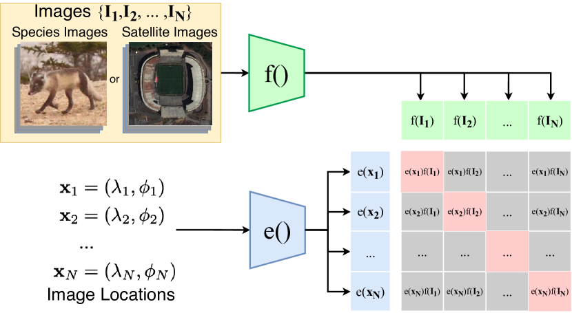
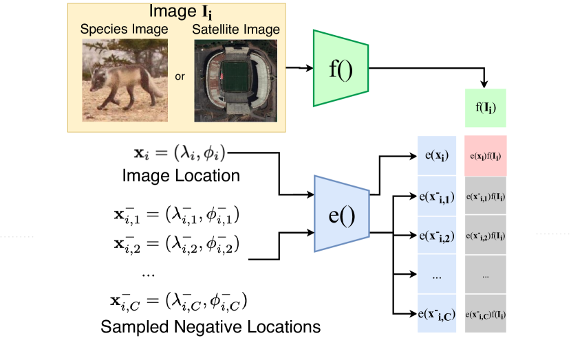
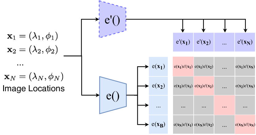
To perform contrastive learning, we explore a combination of three different ways to form positive and negative pairs for the location encoder pre-training stage of CSP as shown in Figure 3: (a) In-batch negative sampling: given a mini-batch of unlabeled location-image pairs, create mismatching location-image pairs as negative samples; (b) Random negative location sampling: uniformly sample negative locations from the study area (e.g., the whole earth surface) to form negative pairs; (c) SimCSE-based sampling: create a positive pair by encoding the same location with two location encoders, which share all the parameters but use different dropout masks. We also compare several self-supervised learning objectives including Mean Square Error loss ($MSE$), Noise Contrastive Estimation loss ($\mathrm{NCE}$), and Contrastive Multi-classification loss ($\mathrm{MC}$).

We conduct experiments on geo-aware image classification tasks including fine-grained species recognition (Chu et al., 2019; Mac Aodha et al., 2019; Mai et al., 2020b; Yang et al., 2022), and remote sensing (RS) image classification (Christie et al., 2018; Ayush et al., 2021; Manas et al., 2021; Li et al., 2021a). Results show that our CSP can boost the model performance on both datasets.

In summary, the contributions of our work are:

• We propose an effective multi-modal self-supervised pre-training method CSP that leverages abundant unlabeled geo-tagged images to better learn location representations that can be transferred to few-shot learning tasks.

• We explore three ways to construct positive and negative training examples for contrastive learning. We find that the combination of them achieves the best performance.

• We explore three self-supervised losses including $MSE$, $\mathrm{NCE}$, and $\mathrm{MC}$. We find out that using CSP with $\mathrm{MC}$ usually yields the best result.

• We apply CSP to fine-grained species recognition (iNat2018) and remote sensing image classification task (fMoW) in few-shot learning and fully supervised settings, and demonstrate advantages on both datasets. CSP can significantly boost model performances with 10-34% relative improvements on the iNat2018 dataset at few-shot settings by stratified sampling $\{5\%,10\%,20\%\}$ of the training data. On both datasets, when training models on the whole training dataset in a fully supervised manner, we find that adding the CSP  pre-training objective can still improve the model performance.

2 Related Work

Unsupervised/Self-Supervised Learning on Geotagged Images

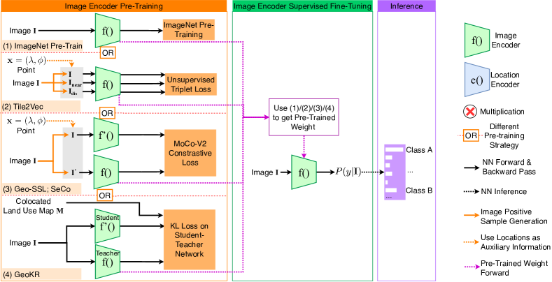
Multiple unsupervised or self-supervised frameworks have been proposed to pre-train image encoder by utilizing geographic knowledge such as Tile2Vec (Jean et al., 2019), Geo-SSL (Ayush et al., 2021), SeCo (Manas et al., 2021), and GeoKR (Li et al., 2021a).

Tile2Vec (Jean et al., 2019) is an unsupervised learning framework to pre-train image encoder based on the spatial relations among RS images. Given an anchor RS image, location information is only used to obtain one nearby tile and a distant tile. An unsupervised triplet loss is formed to pre-train image encoder to make nearby tiles similar in the embedding space while distant tiles dissimilar. Geo-locations are not part of the model input and cannot be used during the model fine-tuning or inference stage.

Geo-SSL (Ayush et al., 2021) is a self-supervised contrastive learning objective to pre-train an RS image encoder based on the MoCo-V2 (Chen et al., 2020b) framework. Instead of using augmented images as positive pairs as MoCo-V2 does, they used co-located RS images at different times as positive pairs. This contrastive image loss is combined with a geo-location classification pre-text loss during pre-training, which uses the image encoder to predict which geo-location cluster the image might come from. Here, the spatiotemporal information is only used in the pre-training stage. During the fine-tuning and inference stage, the model prediction relies entirely on the pre-trained image encoder.

SeCo (Manas et al., 2021) is a similar self-supervised contrastive learning framework for an RS image encoder $f()$. It also uses MoCo-V2 as the backbone and uses spatially aligned RS images at different times as novel temporal augmented samples. The difference is that SeCo uses both the temporal augmented samples and synthetic samples based on artificial augmentations as either positive or negative samples so that the pre-trained $f()$ can be either invariant or sensitive to the temporal or artificial augmentations.

GeoKR (Li et al., 2021a) is proposed as an unsupervised framework for an RS image encoder. GeoKR first obtains a spatially aligned land cover map $\mathbf{M}$ based on an RS image. The image encoder is pre-trained in a teacher-student network to predict the distribution of land cover types in the current scene with a KL loss.

Figure 2(b) illustrates the general idea of those four models while Figure 6 in Appendix A.1 provides a detailed comparison. None of them directly takes geo-locations as model input but use locations as auxiliary information to pre-train the image encoder. Moreover, after pre-training, location information is completely ignored during fine-tuning and inference stage which leads to significantly suboptimal results. In contrast, our CSP utilizes the location-image pairs in a direct and explicit manner by separately encoding them and contrasting them against each other. The pre-trained location encoder can be utilized in the model inference process jointly with the image encoder so that both the visual and spatial clue can be used for prediction.

Location Representation Learning

Zhai et al. (2018) learned location representation from image-location pairs for image localization. So in this context, locations are supervision signals. Instead of using the original geo-locations, they grouped locations (or times) into different bins and utilized them in the cross entropy loss. This practice cannot leverage the continuity of the approximated function. Most existing location encoding approaches (Tang et al., 2015; Christie et al., 2018; Chu et al., 2019; Mac Aodha et al., 2019; Mai et al., 2020b, 2022d; Yang et al., 2022) are developed and trained in a supervised learning framework while massive unlabeled geographic data cannot be used. Figure 2(a) illustrates the dual-encoder supervised learning idea both Mac Aodha et al. (2019) and Mai et al. (2020b) used for geo-aware image classification. In contrast, this work focuses on training location encoders in a self-supervised manner based on unlabeled geotagged images. The pre-trained location encoder can later be utilized jointly with the image encoder for model prediction (See Figure 2(c)).

Spatially Explicit Artificial Intelligence

Previous works showed that naively applying existing state-of-the-art AI models to geospatial tasks usually yielded suboptimal results (Mai et al., 2019; Chu et al., 2019; Mac Aodha et al., 2019; Ayush et al., 2021; Yan et al., 2018). Spatially Explicit Artificial Intelligence aims at improving the performances of AI models on various geospatial tasks by incorporating spatial thinking, spatial principles and spatial inductive biases into the AI model design (Janowicz et al., 2020; Liu & Biljecki, 2022; Zhu et al., 2022; Mai et al., 2022b). Several important spatial principles have been considered by previous works including spatial dependency (Mai et al., 2019; Yan et al., 2018, 2019; Li et al., 2021b; Huang et al., 2022, 2023), spatial heterogeneity (Chu et al., 2019; Mac Aodha et al., 2019; Mai et al., 2020b; Zhu et al., 2021; Xie et al., 2021; Goodchild & Li, 2021; Xie et al., 2023), temporal continuity (Cai et al., 2020; He et al., 2021; Cong et al., 2022), temporal periodicity (Cai et al., 2020; Rao et al., 2020), earth spherical geometry nature (Cohen et al., 2018; Esteves et al., 2018; Jiang et al., 2019; Mai et al., 2022d), and so on. CSP  contributes to the Spatially Explicit Artificial Intelligence research by learning effective multi-scale location representations from unlabeled images.

3 Method

(a) In-batch negative sampling ($B$) Given a batch of unlabeled location-image pairs a $N\times N$ cosine similarity matrix is computed based on all location embeddings and image embeddings.

(b) Random negative location sampling ($L$) Given one positive location-image pair $(\bm{\mathbf{x}}_{i},\mathbf{I}_{i})$, we uniformly sample $C$ negative locations $\{\bm{\mathbf{x}}^{-}_{i,1},\bm{\mathbf{x}}^{-}_{i,2},...,\bm{\mathbf{x}}^{-}_{i,C}\}$ from the study area (e.g., the earth surface) to form negative pairs.

(c) SimCSE sampling ($D$) Two location encoders $e()$ and $e^{\prime}()$ share all the parameters but apply different dropout masks. Given a batch of unlabeled location-image pairs, the same location $\bm{\mathbf{x}}_{i}$ is encoded by $e()$ and $e^{\prime}()$ to form a positive pair, while other pairs are treated as negative examples.

Figure 3: Three different ways to form positive and negative training pairs (red and gray boxes respectively).

3.1 A Dual-Encoder for Geo-Tagged Images

We define an unlabeled geo-tagged image dataset as $\mathbb{X}=\{(\bm{\mathbf{x}}_{i},\mathbf{I}_{i})|i=1,...,M\}$, where $\mathbf{I}_{i}$ is an image, $\bm{\mathbf{x}}_{i}$ represents the location (longitude and latitude) and optionally the time the image was taken. Inspired by recent image-text pre-training models (Zhang et al., 2020; Radford et al., 2021a; Jia et al., 2021; Zhai et al., 2021), CSP uses a dual-encoder architecture – a location encoder $e()$ and an image encoder $f()$ – to handle location $\bm{\mathbf{x}}_{i}$ and image $\mathbf{I}_{i}$ separately.

The location encoder $e()$ is a function $e_{\theta}(\bm{\mathbf{x}}_{i}):\mathbb{S}^{2}\to\mathbb{R}^{d}$, which is parameterized by $\theta$ and maps any coordinate $\bm{\mathbf{x}}_{i}=(\lambda_{i},\phi_{i})$ in a spherical surface $\mathbb{S}^{2}$ to a vector representation of $d$ dimension. Here longitude $\lambda_{i}\in[-\pi,\pi)$ and latitude $\phi_{i}\in[-{\pi}/{2},{\pi}/{2}]$. $e()$ can be any existing 2D location encoders (Mai et al., 2022c) such as $tile$ (Tang et al., 2015), $wrap$ (Mac Aodha et al., 2019), Space2Vec’s $grid$ and $theory$ (Mai et al., 2020b), or spherical location encoders such as Sphere2Vec (Mai et al., 2022d). We assume that $e()$ is inductive and does not depend on the unlabeled dataset $\mathbb{X}$ anymore once it is pre-trained.

The image encoder $f()$ is a function $f_{\psi}(\mathbf{I}_{i}):\mathbb{R}^{H\times W\times C}\to\mathbb{R}^{d}$, which is parameterized by $\psi$ and maps any image with height $H$, width $W$, and channel $C$ into an embedding of $d$ dimension. In this study we define $f(\mathbf{I}_{i})=\mathbf{W}(\mathbb{F}(\mathbf{I}_{i}))$ where $\mathbb{F}()$ is an off-the-shelf deep image neural network such as InceptionV3 (Szegedy et al., 2016) or Geo-SSL (Ayush et al., 2021) pretrained ResNet50 (He et al., 2015), which encodes any image into a $d^{(I)}$ dimension image feature vector. $\mathbf{W}()$ is a projection layer (similar to that of SimCLR (Chen et al., 2020a) and MoCo-V2 (Chen et al., 2020b)), which projects the image feature $\mathbb{F}(\mathbf{I}_{i})\in\mathbb{R}^{d^{(I)}}$ into $d$ dimension such that a contrastive learning objective can be formed between $e(\bm{\mathbf{x}}_{i})$ and $f(\mathbf{I}_{i})$. Please refer to Appendix A.2.1 for a detailed description of $f()$.

In our work, $d^{(I)}=2048$ and $d=512$. This dual-encoder architecture is shown in Figure 2(c) as well as Figure 3. We simply denote the encoded representation of a location $\bm{\mathbf{x}}_{i}$ as $e(\bm{\mathbf{x}}_{i})$ and its associated image representation as $f(\mathbf{I}_{i})$.

3.2 Contrastive Spatial Pre-Training(CSP)

Contrastive Learning Objectives

We consider different contrastive objectives. The first is the noise contrastive estimation (NCE) (Gutmann & Hyvärinen, 2010) loss, which avoids calculation of the partition function and has been successfully used in word embeddings (Mikolov et al., 2013) and language modeling (Mnih & Teh, 2012):

$$\begin{split}l_{\mathrm{NCE}}(\mathcal{P},\mathcal{N})=&-\mathbb{E}_{({\mathbf{a}},{\mathbf{b}})\sim\mathcal{P}}\log\sigma(s({\mathbf{a}},{\mathbf{b}}))\\ &-\mathbb{E}_{({\mathbf{a}},{\mathbf{b}}^{-})\sim\mathcal{N}}\log(1-\sigma(s({\mathbf{a}},{\mathbf{b}}^{-})))\end{split}$$ (1)

Here $\mathcal{P}=\{({\mathbf{a}},{\mathbf{b}})\}$ is a set of positive pairs, and $\mathcal{N}=\{({\mathbf{a}},{\mathbf{b}}^{-})\}$ is a set of negative pairs. $s(\cdot,\cdot)$ is a similarity function (such as $cosine()$), and $\sigma(v)=e^{v}/(1+e^{v})$ is the sigmoid function.

The second objective function is the multi-class classification loss with temperature which takes the same form as the InfoNCE loss (Van den Oord et al., 2018). It has been successfully used in unsupervised learning for images (He et al., 2020) and text (Gao et al., 2021):

$$\begin{split}\small l_{\mathrm{MC}}(\mathcal{P},\mathcal{N},\tau)\\ =\mathbb{E}_{({\mathbf{a}},{\mathbf{b}})\sim\mathcal{P}}&\frac{e^{s({\mathbf{a}},{\mathbf{b}})/\tau}}{e^{s({\mathbf{a}},{\mathbf{b}})/\tau}+\sum_{({\mathbf{a}},{\mathbf{b}}^{-})\in\mathcal{N}_{\mathbf{a}}}e^{s({\mathbf{a}},{\mathbf{b}}^{-})/\tau}}\end{split}$$ (2)

where $\mathrm{MC}$ stands for “multi-class”. $\mathcal{N}_{\mathbf{a}}$ obtains a set of negative pairs with first entry being ${\mathbf{a}}$, $\mathcal{P}$ and $s(\cdot,\cdot)$ are defined as earlier. The temperature scaling parameter $\tau$ determines how soft the softmax is (Hinton et al., 2015). In practice it helps with the trade off between top ranked classes (precision) versus reset of the classes (recall).

Third, we also experimented with a regression loss, but it does not work as well as the NCE and MC losses.

Self-Supervised Training Pair Construction

In order to learn useful representations, we need to choose appropriate distributions for positive pairs $\mathcal{P}$ and negative pairs $\mathcal{N}$ for contrastive learning. In CSP, we use three sampling methods to obtain positive and negative pairs: in-batch negative sampling (indicated as $B$), random negative location sampling (indicated as $L$), and SimCSE-based sampling (indicated as $D$). Figure 3 illustrates how we use these three methods to do the positive and negative sampling. Each of them includes methods to sample both the positive and negative pairs so that one contrastive loss component can be formed based on each of them. Some of them share the same positive sampling method such as $B$ and $L$. So we summarize the positive and negative sampling methods below. Given an unlabeled location-image pair $(\bm{\mathbf{x}}_{i},\mathbf{I}_{i})$ from a mini-batch $\mathbb{X}_{(N)}=\{(\bm{\mathbf{x}}_{1},\mathbf{I}_{1}),(\bm{\mathbf{x}}_{2},\mathbf{I}_{2}),...,(\bm{\mathbf{x}}_{N},\mathbf{I}_{N})\}\subseteq\mathbb{X}$, where $\mathbb{X}$ is a geo-tagged but unlabeled image set, we use the following positive and negative instances:

• Geo-tagged positive $\mathcal{P}^{X}=\{(e(\bm{\mathbf{x}}_{i}),f(\mathbf{I}_{i}))\}$ indicates the original location-image pairs used as positive pairs. This corresponds to the positive pairs used by $B$ and $L$ methods – the red boxes in both Figure 3(a) and 3(b).

• In-batch negatives $\mathcal{N}^{B}=\bigcup_{i}\mathcal{N}^{B}_{i}$, where $\mathcal{N}^{B}_{i}=\{(e(\bm{\mathbf{x}}_{i}),$ $f(\mathbf{I}_{j}))|j\in\{1,2,...,N\}\setminus\{i\}\}$.$\mathcal{N}^{B}$ corresponds to all mismatching location-image pairs in $\mathbb{X}_{(N)}$ – all gray boxes (no-diagonal elements) in Figure 3(a).

• Sampled negative locations $\mathcal{N}^{L}=\bigcup_{i}\mathcal{N}^{L}_{i}$, where $\mathcal{N}^{L}_{i}=\{(e(\bm{\mathbf{x}}^{-}_{i,j}),$ $f(\mathbf{I}_{i}))|j\in\{1,2,...,C\}\}$ indicates $C$ negative pairs for $\mathbf{I}_{i}$. Note that $\bm{\mathbf{x}}^{-}_{i,j}$ is sampled uniformly from the surface of the sphere at pre-training time, and therefore they are different at each training epoch. $\mathcal{N}^{L}$ corresponds to all gray boxes in Figure 3(b). This is a common negative location sampling practice used by Mac Aodha et al. (2019); Mai et al. (2020b).

• Dropout positive $\mathcal{P}^{D}=\{(e(\bm{\mathbf{x}}_{i}),e^{\prime}(\bm{\mathbf{x}}_{i}))\}$, where given two towers of the same location encoders $e()$ and $e^{\prime}()$ with two independently sampled dropout masks, we pass the same input $\bm{\mathbf{x}}_{i}$ to them and obtain two embeddings $(e(\bm{\mathbf{x}}_{i}),e^{\prime}(\bm{\mathbf{x}}_{i}))$ as “positive pairs”. This is a data augmentation strategy (so called SimCSE), which has been very successful for sentence embeddings (Gao et al., 2021). This corresponds to the red boxes in Figure 3(c).

• Dropout negative $\mathcal{N}^{D}=\bigcup_{i}\mathcal{N}^{D}_{i}$, where $\mathcal{N}^{D}_{i}=\{(e(\bm{\mathbf{x}}_{i}),$ $e^{\prime}(\bm{\mathbf{x}}_{j}))|j\in\{1,2,...,N\}\setminus\{j\}\}$. $\mathcal{N}^{D}$ indicates the location embeddings from two location encoder towers based on different locations from the same mini-batch. It corresponds to the gray boxes in Figure 3(c).

As shown in Figure 3, those five positive/negative sampling sets amount to three different sampling methods:

• In-batch negative sampling ($B$) (Zhang et al., 2020; Radford et al., 2021b; Carlsson et al., 2021; Karpukhin et al., 2020) uses $\mathcal{P}^{X},\mathcal{N}^{B}$ as positive and negative pairs.

• Random negative location sampling ($L$) (Mac Aodha et al., 2019; Mai et al., 2020b, 2022d) uses $\mathcal{P}^{X},\mathcal{N}^{L}$ as positive and negative pairs.

• SimCSE-based sampling ($D$) (Gao et al., 2021) uses $\mathcal{P}^{D},\mathcal{N}^{D}$ as positive and negative pairs. Please refer to Appendix A.3 for a detailed description.

Each corresponds to one loss component in our contrastive learning loss function by using either $\mathrm{NCE}$ or $\mathrm{MC}$ objective shown in Equation 1 and 2. So we define two versions of contrastive losses which both have three components.

The self-supervised binary ($\mathrm{NCE}$) loss $l_{\mathrm{NCE}}$ is defined as

$$\begin{split}l_{\mathrm{NCE}}(\mathbb{X})&=l_{\mathrm{NCE}}^{B}(\mathbb{X})+\beta_{1}l_{\mathrm{NCE}}^{L}(\mathbb{X})+\beta_{2}l_{\mathrm{NCE}}^{D}(\mathbb{X})\\ &=l_{\mathrm{NCE}}(\mathcal{P}^{X},\mathcal{N}^{B})+\beta_{1}l_{\mathrm{NCE}}(\emptyset,\mathcal{N}^{L})\\ &+\beta_{2}l_{\mathrm{NCE}}(\mathcal{P}^{D},\mathcal{N}^{D})\end{split}$$ (3)

where $\beta_{1}$ and $\beta_{2}$ control the contribution of the last two loss components. Note here we use empty set as the positive pairs in $l_{\mathrm{NCE}}^{L}(\mathbb{X})$ since $\mathcal{P}^{X}$ has been considered in $l_{\mathrm{NCE}}^{B}(\mathbb{X})$.

The self-supervised multi-class ($\mathrm{MC}$) loss $l_{\mathrm{MC}}$ is defined as

$$\begin{split}l_{\mathrm{MC}}(\mathbb{X})=&l_{\mathrm{MC}}^{B}(\mathbb{X})+\alpha_{1}l_{\mathrm{MC}}^{L}(\mathbb{X})+\alpha_{2}l_{\mathrm{MC}}^{D}(\mathbb{X})\\ =&l_{\mathrm{MC}}(\mathcal{P}^{X},\mathcal{N}^{B},\tau_{0})+\alpha_{1}l_{\mathrm{MC}}(\mathcal{P}^{X},\mathcal{N}^{L},\tau_{1})\\ &+\alpha_{2}l_{\mathrm{MC}}(\mathcal{P}^{D},\mathcal{N}^{D},\tau_{2})\end{split}$$ (4)

where $\alpha_{1}$ and $\alpha_{2}$ are hyper-parameters. Although $l_{\mathrm{MC}}^{B}(\mathbb{X})$ and $l_{\mathrm{MC}}^{L}(\mathbb{X})$ use the same positive pairs $\mathcal{P}^{X}$, they are embedded in the Softmax function. So we need to use $\mathcal{P}^{X}$ in both loss components.

A naive contrastive pre-training for this dual-encoder architecture is to jointly training both encoders from scratch as CLIP (Radford et al., 2021a) and ALIGN (Jia et al., 2021) do for the image and text encoder. However, from-scratch training will be problematics in CSP. Unlike CLIP and ALIGN’s dual-encoder framework in which the text and image encoder have relatively the same number of trainable parameters, the number of trainable parameters of the image encoder $f()$ is 100 times larger than that of the location encoder $e()$. For example, the InceptionV3 image encoder we used for iNat2018 dataset has 41.8 million trainable parameters while the Space2Vec location encoder we used in both iNat2018 and fMoW dataset has only 0.4 million trainable parameters. Jointly training both encoders from scratch will yield overfitting issue for location encoder and underfitting issue for the image encoder.

Moreover, in text-image pre-training literature, LiT (Zhai et al., 2021) also reported that locking the image encoder during pre-training leads to a significant performance improvement. So we follow the practice of LiT (Zhai et al., 2021), and utilize a pre-trained image network $\mathbb{F}^{*}()$ and lock it during Contrastive Spatial Pre-Training. The pre-trained image network $\mathbb{F}^{*}()$ should not see the current image labels during pre-training stage. In other words, we first do image encoder pre-training as shown in the orange box of Figure 2(c). Then we lock $f()$ and use it to pre-train $e()$ as shown in the red box of Figure 2(c). During CSP, only the image projection layer $\mathbf{W}()$ is trained in the image encoder part.

3.3 Supervised Fine-Turning

After Contrastive Spatial Pre-Training, we follow the practice of Chu et al. (2019); Mac Aodha et al. (2019); Mai et al. (2022d) and fine-tune the image encoder $f()$ and location encoder $e()$ separately on a small labeled dataset $\overline{\mathbb{X}}=\{(\bm{\mathbf{x}},\mathbf{I},y)\}$ to test its performance in a few-shot learning setting. The supervised fine-tuning stage corresponds to the green and blue box in Figure 2(c). Their predictions are combined at the inference stage as Mac Aodha et al. (2019); Mai et al. (2020b, 2022d) did.

Image Encoder Fine Tuning

We drop the projection layer $\mathbf{W}()$ and use a classification head $g()$ to process the image feature vector $\mathbb{F}(\mathbf{I})$ into logits over image labels, i.e., $g(\mathbb{F}(\mathbf{I}))\in\mathbb{R}^{Q}$. We fine-tune $g()$ with cross-entropy loss. $Q$ is the total number of classes. This process corresponds to the green box in Figure 2(c). Please refer to Appendix A.2.1 for a detailed description of $f()$ fine-tuning.

Location Encoder Fine Tuning

As shown in the blue box of Figure 2(c), we use image labels in the training objective for location encoder fine tuning. Following Mac Aodha et al. (2019), we used a presence-absence loss function which converts the multi-class labels into binary multi-labels. A class embedding matrix $\mathbf{T}\in\mathbb{R}^{d\times Q}$ is used to supervisedly train the location encoder where $\mathbf{T}_{:,y}\in\mathbb{R}^{d}$ indicates the class embedding for the $y$th class. Given a set of training samples $\overline{\mathbb{X}}=\{(\bm{\mathbf{x}},\mathbf{I},y)\}$ where $y$ indicates the class label, the loss function $l^{sup}(\overline{\mathbb{X}})$ is defined as:

$$\begin{split}l^{sup}(\overline{\mathbb{X}})=\beta l_{\mathrm{NCE}}(\mathcal{P}^{y},\emptyset)+l_{\mathrm{NCE}}(\emptyset,\mathcal{N}^{y}\cup\mathcal{N}^{R})\end{split}$$ (5)

Here $\beta$ is a hyperparameter for the weight of positive samples. The following positive and negative samples are used:

• Labeled positives $\mathcal{P}^{y}=\{(e(\bm{\mathbf{x}}),\mathbf{T}_{:,y})|(\bm{\mathbf{x}},y)\in\overline{\mathbb{X}}\}$.

• Labeled negatives $\mathcal{N}^{y}=\{(e(\bm{\mathbf{x}}),\mathbf{T}_{:,y_{j}})|(\bm{\mathbf{x}},y)\in\overline{\mathbb{X}},y_{j}\in\{1..Q\}\setminus\{y\}\}$.

• Sampled negative locations $\mathcal{N}^{R}=\{(e(\bm{\mathbf{x}}^{-}),\mathbf{T}_{:,y_{j}})|(\bm{\mathbf{x}},y)\in\overline{\mathbb{X}},\;y_{j}\in\{1..Q\}\}$, where $\bm{\mathbf{x}}^{-}$ is a uniformly sampled locations from the surface of the sphere for each example $\bm{\mathbf{x}}$.

3.4 Model Inference

At inference time, we combined the predicted logits of fine-tuned $e()$ and $f()$ to give the final prediction as shown in the purple box of Figure 2(c). Given a location-image pair $(\bm{\mathbf{x}},\mathbf{I})$, we estimate which category $y$ it belongs to by $P(y|\mathbf{I},\bm{\mathbf{x}})$. According to Mac Aodha et al. (2019), if we assume $\mathbf{I}$ and $\bm{\mathbf{x}}$ are conditionally independent given $y$, then based on Bayes’ theorem, we have $P(y|\mathbf{I},\bm{\mathbf{x}})\;\propto\;P(y|\bm{\mathbf{x}})P(y|\mathbf{I})$. Here, $P(y|\mathbf{I})$ can be estimated by the logits of $g(\mathbb{F}(\mathbf{I}))$ at the $y$th class. For $P(y|\bm{\mathbf{x}})$, we have $P(y|\bm{\mathbf{x}})\;\propto\;\sigma(e(\bm{\mathbf{x}})\mathbf{T}_{:,y})$ where $\sigma(\cdot)$ is a sigmoid activation function.

4 Experiments

In this work, we study the effectiveness of CSP on two geo-aware image classification tasks - species fine-grained recognition and satellite image classification. We are particularly interested in how the dual-encode architecture performs in various few-shot learning settings after CSP.

For each task, three datasets are used to pre-train, fine-tune, and evaluate our CSP  models: $\mathbb{X}_{train}$ is a set of unlabeled location-image pairs we use for pre-training; $\overline{\mathbb{X}}_{train}$ is a set of labeled location-image-class tuples we use for fine-tuning, where the size of $\mathbb{X}_{train}$ is much larger than that of $\overline{\mathbb{X}}_{train}$, i.e., $|\mathbb{X}_{train}|\gg|\overline{\mathbb{X}}_{train}|$; and $\overline{\mathbb{X}}_{val}$ is a set of labeled location-image-class tuples we use for evaluation that can not be seen during fine-tuning.

4.1 Models and Baselines

In this work, we consider the following baselines:

• Img. Only supervisedly fine-tune the image network $g(\mathbb{F}())$ on the fine tuning dataset $\overline{\mathbb{X}}_{train}$ (See Figure 2(b)). We use InceptionV3 (Szegedy et al., 2016) and ResNet50 (Ayush et al., 2021) as the image encoders on iNat2018 and fMoW respectively.

• Sup. Only uses the dual-encoder architecture but is only supervisedly trained on $\overline{\mathbb{X}}_{train}$ (See Figure 2(a)). We consider use $wrap$ (Mac Aodha et al., 2019) and $grid$ (Mai et al., 2020b) as the location encoder which yield two models: Sup. Only (wrap) and Sup. Only (grid).

• MSE follows the same setup as CSP (See Figure 2(c)) except that during location encoder pre-training, it directly feeds the location embedding $e(\bm{\mathbf{x}})$ into a linear layer to regress the image feature vector $\mathbb{F}(\mathbf{I})$ with a Mean Square Error (MSE) loss. MSE uses $grid$ as the location encoder.

We compare these baselines with different versions of CSP. All CSP  models have the same training procedure, and use $grid$ as their location encoders. The only difference is the contrastive loss function they use:

• CSP-NCE-BLD uses the $\mathrm{NCE}$ loss with all three loss components as shown in Equation 3.

• CSP-MC-BLD uses the $\mathrm{MC}$ loss with all three loss components as shown in Equation 4.

4.2 Fine-Grained Species Recognition

We use the iNat2018 dataset (Van Horn et al., 2018) as a representative dataset to study the effectiveness of CSP  on species fine-grained recognition. iNat2018 is a large-scale species classification dataset with 8142 species categories. There are 437,513 training images of which 436,063 training images have geo-locations. On average each class has 53.6 training samples. We use all location-image pairs $\{(\bm{\mathbf{x}}_{i},\mathbf{I}_{i})\}$ in iNat2018 training set as the unlabeled geo-tagged dataset $\mathbb{X}_{train}$ for our CSP. To create a few-shot learning task, we perform a stratified sampling on the training dataset to select $\lambda\%$ of training samples which constitute our few-shot supervised fine-tuning dataset $\overline{\mathbb{X}}_{train}=\{(\bm{\mathbf{x}},\mathbf{I},y)\}$. The iNat2018 validation dataset is used for model evaluation to make our results comparable with previous work (Mac Aodha et al., 2019; Mai et al., 2020b, 2022d). We use InceptionV3 network pre-trained on ImageNet as the image feature extractor $\mathbb{F}^{*}()$ for iNat2018 dataset.

Table 1 compares the Top1 accuracy of different training strategies on the iNat2018 validation dataset with different $\lambda\%$. From Table 1, we can see that:

• Img. Only (ImageNet) yields the lowest performances in all $\lambda\%$ settings which indicates that considering location information is beneficial in all settings.

• Sup. Only (grid) outperforms Sup. Only (wrap) across all settings indicating that multi-scale location encoders (e.g., grid) are effective for spatial distribution modeling. This confirms the results of Mai et al. (2020b).

• Comparing the last three models, we can see the general patterns in all $\lambda\%$ settings: CSP-MC-BLD> CSP-NCE-BLD> MSE. Since these three models only differ in terms of the location encoder pre-training strategies (the red box in Figure 2(c)), this indicates that CSP-MC-BLD is the best location encoder pre-training objective.

• When $\lambda\%=5\%,10\%,20\%$, compared with the Sup. Only, CSP-MC-BLD have relative performance improvements of 10.4%, 34.3%, and 16.6% which indicates the effectiveness of Contrastive Spatial Pre-Training.

• When $\lambda\%=100\%$, CSP-MC-BLD still yields better results than Sup. Only (grid). This indicates that our ${CSP}$ is beneficial even in a fully supervised setting.

To understand the effectiveness of each loss component in CSP (see Figure 3 and Equation 4), we conduct an ablation study on the iNat2018 dataset with different $\lambda$ and report the results in Table 2. We can see that each component contributes to the final model performance. Deleting any of them will lead to performance drops.

To understand the effect of location embedding dimension $d$ on the model performance, we conduct an additional ablation study of $d$ on the iNat2018 dataset with different $\lambda$ and report the results in Table 3. We can see that at the few-shot setting $\lambda\%=5\%,10\%,20\%$, models with $d=256$ achieve the best performance. In the fully supervised setting, the model with $d=1024$ leads to the best performance.

Last but not least, we also explore whether our CSP is effective on different image encoders. We conduct an ablation study of different $\mathbb{F}()$ on the iNat2018 dataset with $\lambda\%=5\%$. Table 4 summarizes the results. We can see that no matter which $\mathbb{F}()$ we use, Inception V3 or ViT, our CSP-MC-BLD consistently yields the best results, and ViT improves the model performance a lot.

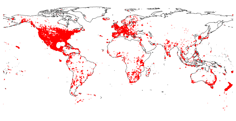
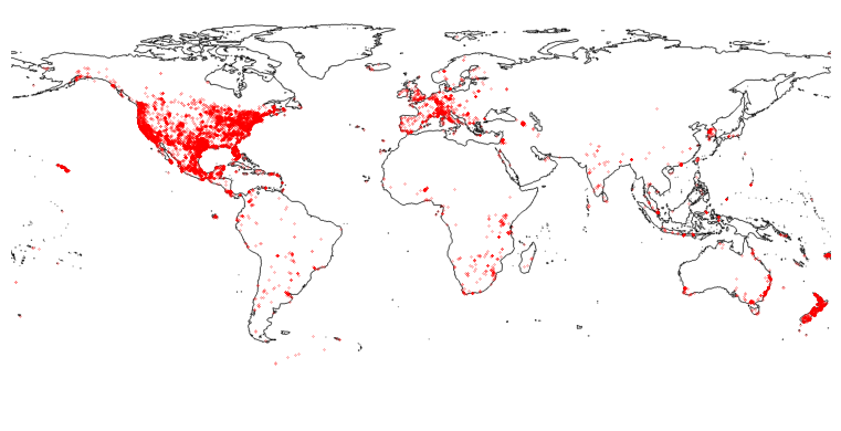
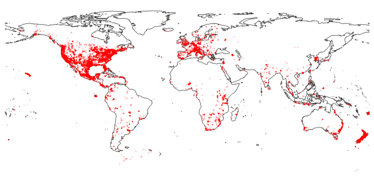
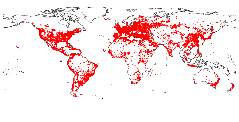
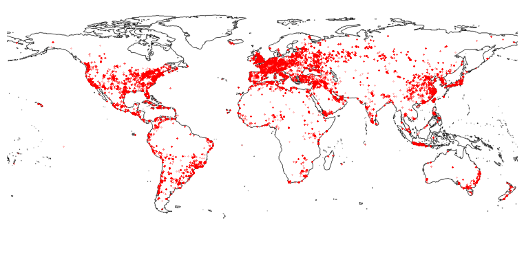
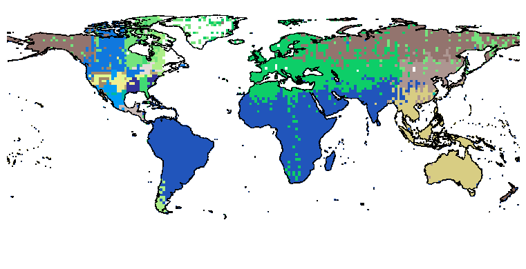
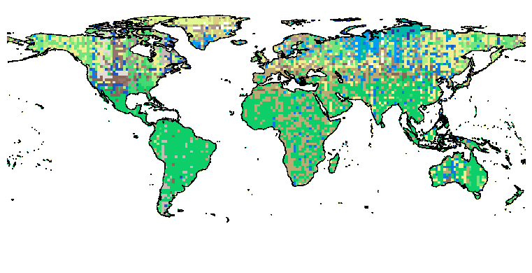
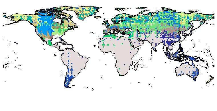
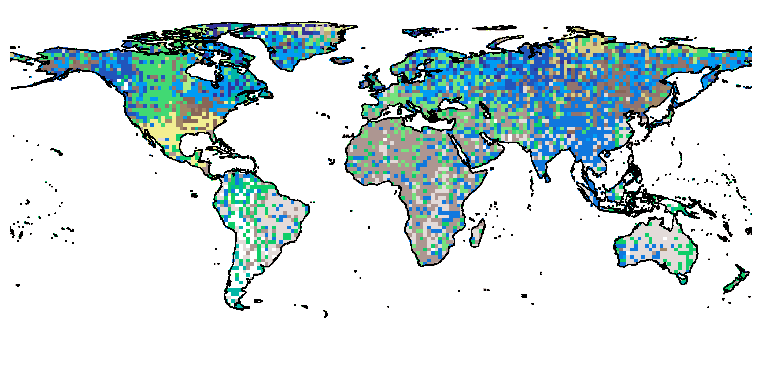
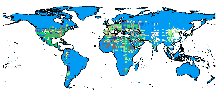
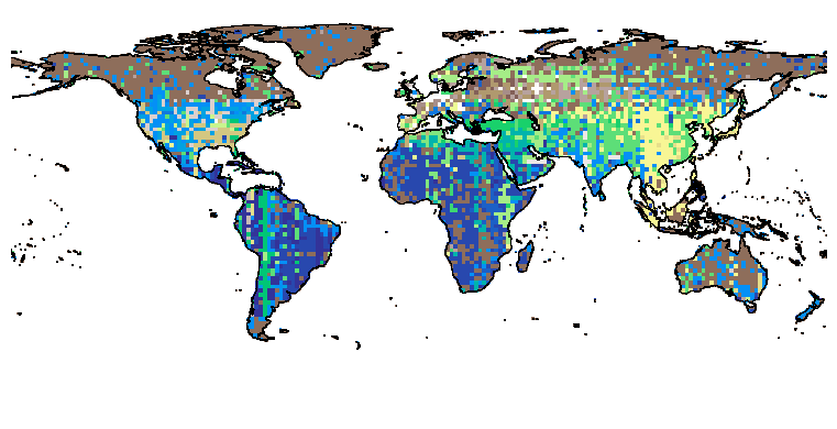
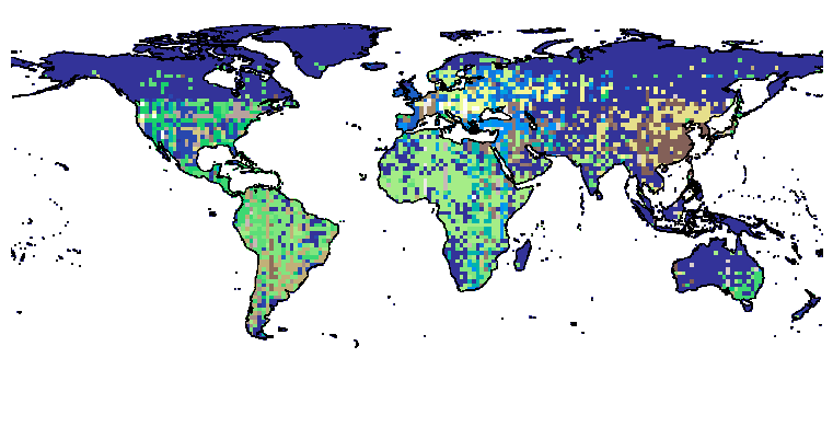
To investigate how well CSP  learns location representation, we sample a set of regular grid points all over the world and compute their embeddings with the location encoder $e()$. The resulting location embeddings are hierarchically clustered. The results are shown in Figure 4. Figure 4(a) and 4(c) show the clustering results after CSP-MC-BLD or CSP-NCE-BLD pre-training, while Figure 4(b) and 4(d) show the clustering results after supervised fine-tuning on respective models. Some interesting clustering patterns merge in Figure 4(a) and 4(c). For example, the clustering patterns in Figure 4(a) show some regional effects that are somewhat similar to the Köppen climate classification. This makes sense since the pre-training with location-image pairs is learning the spatial distribution of species and their environment, which is highly related to climate zones. The clusters in the US are smaller since the iNat2018 training dataset has much more data in the US (See Figure 8(a) in Appendix A.7).

Table 1: The Top1 accuracy of different models and training strategies on the iNat2018 validation dataset for the species fine-grain recognition task with different training data ratios, where $\lambda\%=100\%$ indicates the fully supervised setting. We run each model 5 times and report the standard deviation in “()”.

Ratio $\lambda\%$	5%	10%	20%	100%
Img. Only (ImageNet) (Szegedy et al., 2016)	5.28 (-)	12.44 (-)	25.33 (-)	60.2 (-)
Sup. Only (wrap) (Mac Aodha et al., 2019)	7.12 (0.02)	12.50 (0.02)	25.36 (0.03)	72.41 (-)
Sup. Only (grid) (Mai et al., 2020b)	8.16 (0.01)	14.65 (0.03)	25.40 (0.05)	72.98 (0.04)
MSE	8.15 (0.02)	17.80 (0.05)	27.56 (0.02)	73.27 (0.02)
CSP-NCE-BLD	8.65 (0.02)	18.75 (0.12)	28.15 (0.07)	73.33 (0.01)
CSP-MC-BLD	9.01 (0.02)	19.68 (0.05)	29.61 (0.03)	73.79 (0.02)

Table 2: Ablation studies on different CSP-MC-* pretraining objectives on the iNat2018 validation dataset with different $\lambda\%$. Here, CSP-MC-BLD indicates the CSP training on the $\mathrm{MC}$ loss with all three components. CSP-MC-BL deletes the SimCSE $l_{\mathrm{MC}}^{D}(\mathbb{X})$ component in Equation 4. The rest models follow similar logic.

Ratio $\lambda\%$	5%	10%	20%	100%
CSP-MC-BLD	9.01	19.68	29.61	73.79
CSP-MC-BD	8.63	19.60	29.52	73.15
CSP-MC-BL	8.40	17.17	26.63	73.36
CSP-MC-B	8.16	16.58	25.89	73.10

Table 3: Ablation studies on different location embedding dimensions $d$ on the iNat2018 validation dataset with different $\lambda\%$.

	$d$	5%	10%	20%	100%
CSP-MC-BLD	64	7.64	16.57	25.31	71.76
CSP-MC-BLD	128	8.5	19.35	29.11	72.89
CSP-MC-BLD	256	9.01	19.68	29.61	73.62
CSP-MC-BLD	512	8.97	18.8	27.96	73.67
CSP-MC-BLD	1024	8.78	17.94	26.65	73.79

Table 4: Ablation studies on different image neural network $\mathbb{F}()$ (InceptionV3 (Szegedy et al., 2016) and ViT (Dosovitskiy et al., 2021)) on the iNat2018 validation dataset with $\lambda\%=5\%$.

$\mathbb{F}()$	Inception V3	ViT
Img. Only (ImageNet) (Szegedy et al., 2016)	5.28	12.46
Sup. Only (wrap) (Mac Aodha et al., 2019)	7.12	18.66
Sup. Only (grid) (Mai et al., 2020b)	8.16	18.68
MSE	8.15	20.02
CSP-NCE-BLD	8.65	20.16
CSP-MC-BLD	9.01	20.78

Table 5: The Top1 accuracy of different models and training strategies on the fMoW val dataset for the satellite image classification task with different training data ratios, where $\lambda\%=100\%$ indicates fully supervised setting. We report the standard errors (SE) over 5 different runs.

Ratio $\lambda\%$	5%	10%	20%	100%
Img. Only (Tile2Vec) (Jean et al., 2019)	59.41 (0.23)	61.91 (0.31)	62.96 (0.51)	64.45 (0.37)
Img. Only (Geo-SSL) (Ayush et al., 2021)	65.22 (-)	66.46 (-)	67.66 (-)	69.83 (-)
Sup. Only (wrap) (Mac Aodha et al., 2019)	66.67 (0.03)	68.22 (0.01)	69.45 (0.01)	70.30 (0.02)
Sup. Only (grid) (Mai et al., 2020b)	67.01 (0.02)	68.91 (0.04)	70.20 (0.03)	70.77 (0.03)
MSE	67.06 (0.04)	68.90 (0.05)	70.16 (0.02)	70.45 (0.01)
CSP-NCE-BLD	67.29 (0.03)	69.20 (0.03)	70.65 (0.02)	70.89 (0.04)
CSP-MC-BLD	67.47 (0.02)	69.23 (0.03)	70.66 (0.03)	71.00 (0.02)

(a) MC Unsupervised

(b) MC Supervised

(c) NCE Unsupervised

(d) NCE Supervised

Figure 4: Location embedding before and after supervised fine-tuning for iNat2018.

(a) MC Unsupervised

(b) MC Supervised

(c) NCE Unsupervised

(d) NCE Supervised

Figure 5: Location embedding before and after supervised fine tuning for fMOW.

4.3 Satellite Image Classification

A similar procedure is carried out on fMoW dataset (Christie et al., 2018), which has 62 different geospatial object classes, and 363,570 location-image pairs. We use all location-image pairs as $\mathbb{X}_{train}$, and stratified sample $\lambda\%$ labeled location-image pairs from the training dataset as $\overline{\mathbb{X}}_{train}$. We use similar training, and evaluation protocol as Section 4.2. The ResNet50 checkpoint after Geo-SSL’s MoCo-V2+TP self-supervised pre-training on unlabeled fMoW dataset (Ayush et al., 2021) is used as the pre-trained image feature extractor $\mathbb{F}^{*}()$ for all models.

Table 5 compares the evaluation results (Top1 accuracy) among different models and training strategies on the fMoW val dataset after fine-tuning on $\lambda\%$ fMoW training samples where $\lambda\%\in\{5\%,10\%,20\%,100\%\}$. We can see that Table 5 shows similar patterns as those of Table 1:

• Img. Only (Geo-SSL) yields better results than Img. Only (Tile2Vec) across different $\lambda\%$. But both Img. Only models still give the lowest performance than all other settings with all $\lambda\%$. This confirms the importance of jointly learning location representations. However, Img. Only (Geo-SSL) gives a relatively good performance (65.22%) even when $\lambda\%=5\%$. That is because we use the Geo-SSL’s MoCo-V2+TP checkpoint which is directly pre-trained on the unlabeled fMoW training dataset. In contrast, in Table 1, Img. Only used an InceptionV3 model pre-trained on ImageNet, not on the iNat2018 training dataset.

• Similar to the results in Table 1, Sup. Only (grid) outperforms Sup. Only (wrap) in all settings which shows the effectiveness of grid over wrap.

• CSP-MC-BLD outperforms all models and yields super or comparable results of CSP-NCE-BLD. However, the margins are relatively small compared with those of Table 1. The performance improvements mainly come from the location encoder’s ability to do spatial distribution modeling. Compared with species distribution, the geographic distributions of land use types are very complex and hard to differentiate from each other. For example, factories and multi-unit residential buildings are both man-made geographic entities. Both their distributions are correlated with population distributions and are hard to differentiate. Moreover, sometimes they also show similar appearance in remote sensing images. So it is rather hard to use a location encoder to differentiate one land use type from the other based on their geographic distribution. We think a more powerful location encoding is needed to differentiate them. But this is beyond the scope of this paper.

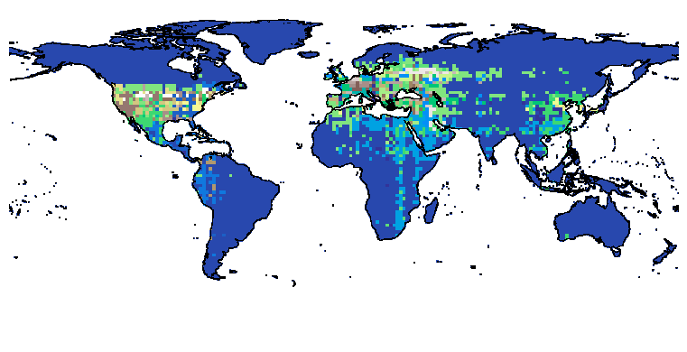
Similar to the iNat2018 dataset, in the fMoW dataset, the embedding clustering results of the pre-trained and fine-tuned location encoders are visualized in Figure 5. We can see that more fine-grained clusters are generated in the US after CSP-MC-BLD/CSP-NCE-BLD pre-training, while the representation is updated to be more detailed after location encoder fine-tuning. Compared with Figure 4, the regional effect is less clear which also shows the difficulty to model the spatial distributions of land use types.

5 Conclusion and Discussion

In this work, we proposed Contrastive Spatial Pre-Training (CSP), a self-supervised framework to learn the alignment between locations and images based on large unlabeled geo-tagged images. Similar to recent popular image-text pre-training models such as CLIP and ALIGN, CSP  utilizes a dual-encoder architecture to separately encode the location and image. The resulting location and image representation are contrasted against each other to form a contrastive pre-training objective. To validate the effectiveness of CSP, we conduct experiments on two geo-aware image classification tasks: species fine-grained recognition on iNat2018 dataset and satellite image classification on the fMoW dataset. Experiments results show that CSP can improve model performance on both datasets under different labeled training data sampling ratios. On the iNat2018 dataset CSP can significantly boost the model performance with 10-34% relative improvement in several few-shot settings ( $\lambda\%=\{5\%,10\%,20\%\}$) and still be able to improve model performance when $\lambda=100\%$.

To the best of our knowledge, our work is the first one to show the great potential of learning the geospatial-visual alignment for model pre-training. Although we only investigate the effectiveness of our CSP framework on location-image pre-training in this work, CSP  can be easily extended to learn the alignment between location (or time) and data in other modalities such as text for different downstream tasks such as geo-aware text classification. We put this as one of our future works. Moreover, in this work, we only use the existing geo-tagged datasets (e.g., iNat2018 and fMoW) as a proxy for unlabeled location-image pairs. In the future, we would like to construct larger-scale unlabeled geo-tagged image datasets based on publicly available satellite images with which we expect to see a larger performance improvement. In this work, we only use single geo-coordinates for geospatial-visual contrastive representation learning. In the future, we can explore more complex geometries such as polylines (Xu et al., 2018) and polygons (Mai et al., 2023b). The proposed CSP  framework can be seen as a step towards the multimodal foundation models for geospatial artificial intelligence (Mai et al., 2022a, 2023a).

6 Ethics Statements

Our code and used datasets are available from https://gengchenmai.github.io/csp-website/. We do not find any negative societal impact of our research.

Appendix A Appendix

A.1 A Detailed Version of Figure 2(b)

Figure 6: A detailed version of Figure 2(b) to show four different ways to pretrain image encoder $f()$ (orange box): (1) ImageNet Pretraining (Deng et al., 2009): pre-training $f()$ on ImageNet dataset; (2) Tile2Vec (Jean et al., 2019): pretraining $f()$ with an unsupervised triplet loss such that the embeddings of spatially nearby image tiles are more similar than those of distant tiles. (3) Geo-SSL (Ayush et al., 2021) and SeCo(Manas et al., 2021): pretraining $f()$ with a Momentum Contrast (MoCo-v2) (Chen et al., 2020c) style constrastive loss in which they used locations as auxiliary information to generate spatially aligned (remote sensing) images at different timestamps as positive samples; (4) GeoKR (Li et al., 2021a): pretraining $f()$ in a teacher-student network by minimizing the KL (Kullback–Leibler) loss between the image representations and a spatially aligned auxiliary data such as land cover maps $\mathbf{M}$. The pre-trained weights of $f()$ are fine-tuned in a supervised manner (green box) for image classification. Here, location is only used as auxiliary information for image encoder pre-training while being ignored during supervised learning stage.

A.2 Model Architecture Training Detail

A.2.1 Training Details of Image Encoder $f()$

Figure 7: A detailed illustration of the image encoder $f()$ we use in Figure 2 for model pre-training and fine-tuning.

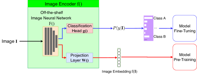
Figure 7 is a detailed illustration of how we use the image encoder $f()$ for model pre-training and fine-tuning. On both iNat2018 and fMoW dataset, we use off-the-shelf image neural network $\mathbb{F}()$ to first encode the given image $\mathbf{I}$ into a $d^{(I)}$ dimension image feature vector $\mathbb{F}(\mathbf{I})\in\mathbb{R}^{d^{(I)}}$. On the iNatlist dataset, two pre-trained image models are used – 1) ImageNet pre-trained InceptionV3 (Szegedy et al., 2016) from PyTorchVision library and 2) ImageNet pre-trained Vision Transformer (ViT) (Dosovitskiy et al., 2021) from Huggingface timm library. See Table 4 for the performance comparison of these two models. On the fMoW dataset, we use Geo-SSL (Ayush et al., 2021) pretrained ResNet50 (He et al., 2015) as $\mathbb{F}()$.

During the CSP  pre-training stage, we feed $\mathbb{F}(\mathbf{I})$ into a projection layer $\mathbf{W}()$ which projects the image feature $\mathbb{F}(\mathbf{I}_{i})\in\mathbb{R}^{d^{(I)}}$ into $d$ dimension such that a contrastive learning objective can be formed between $e(\bm{\mathbf{x}}_{i})$ and $f(\mathbf{I}_{i})$. This illustrates as red arrows in Figure 7.

During the image encoder fine-tuning stage, we drop the projection layer $\mathbf{W}()$ and append a classification head $g()$ to the end of $\mathbb{F}()$ which maps the image feature vector $\mathbb{F}(\mathbf{I})$ into logits over each image label, i.e., $g(\mathbb{F}(\mathbf{I}))\in\mathbb{R}^{Q}$. $Q$ is the total number of classes. This illustrates as blue arrows in Figure 7. Here, both $\mathbf{W}()$ and $g()$ are implemented as multi-layer perceptrons. In practice, on the iNat2018 dataset, we fine-tune the whole image encoder $g(\mathbb{F}(\mathbf{I}))$ instead of only linear probing the $g()$ because 1) both used Inception V3 and ViT image neural network are previously pre-trained on ImageNet dataset whose images are different from the images in iNat2018; 2) Empirical experiments show that fine-tuning the whole architecture yields better performances; 3) The same practice was adopted by Mac Aodha et al. (2019); Mai et al. (2020b). On the fMoW dataset, we use Geo-SSL (Ayush et al., 2021) pretrained ResNet50 (He et al., 2015) and only linear probe on the $g()$. That is because the used $\mathbb{F}()$ is self-supervised pre-trained on the same dataset.

A.2.2 Training Details of Location Encoder $e()$

In terms of the location encoder, we use the Space2Vec grid (Mai et al., 2020b) as the location encoder for both datasets except for Img. Only and Sup. Only (wrap) model. Img. Only does not use location encoders and Sup. Only (wrap) uses wrap location encoder.

During model pre-training, after pre-training the image encoder $f()$, we lock $f()$ and use it to pre-train $e()$ as shown in the red box of Figure 2(c). Location encoder fine-tuning details have been described in Section 3.3

A.2.3 Model Implementation Details

All models are implemented in PyTorch and trained on a Linux machine with 252GB memory and two GeoForce CUDA cores. The code, data, and pre-trained models of this work are all available at https://gengchenmai.github.io/csp-website/.

A.3 Implementation Details of SimCSE

The implementation of SimCSE shown in Figure 3(c) is inspired by Gao et al. (2021). Basically, we have initialized two location encoder towers with identical structures. They share the parameters but they use independently sampled dropout masks. The two dropout masks are sampled independently for every training examples during CSP pretraining. The masks are automatically generated by the dropout layers.

In the implementation, we simply feed the same location $\bm{\mathbf{x}}_{i}$ to the same location encoder twice and get two location embeddings $e(\bm{\mathbf{x}}_{i})$ and $e^{\prime}(\bm{\mathbf{x}}_{i})$. Since they are based on two separate forward passes, they are based on different dropout masks. When we obtain $e^{\prime}(\bm{\mathbf{x}}_{i})$, we not only get the location embedding for $\bm{\mathbf{x}}_{i}$ but also get embeddings for all locations in the same mini-batch. Among all these locations in the mini-batch, we select the embedding of location $\bm{\mathbf{x}}_{j}$ – $e^{\prime}(\bm{\mathbf{x}}_{j})$ where $j\neq i$. Since $e^{\prime}(\bm{\mathbf{x}}_{j})$ and $e^{\prime}(\bm{\mathbf{x}}_{i})$ are generated based on the same forward pass, they share the same dropout mask. So the pair $(e(\bm{\mathbf{x}}_{i}),e^{\prime}(\bm{\mathbf{x}}_{i}))$ is the dropout positive sample (the only difference is the dropout mask) and $(e(\bm{\mathbf{x}}_{i}),e^{\prime}(\bm{\mathbf{x}}_{j}))$ is the negative pair who use different dropout masks and encode different input locations. In short, SimCSE simply uses dropout as a data augmentation tool to generate positive samples.

A.4 Model Hyperparameter Tuning

Since the self-supervised learning takes very long time to tune and hard to evaluate, we first perform a grid search to tune the hyperparameters related to supervised fine tuning stage for the location encoder without self-supervised pre-training. In other words, we tune those hyperparameters on the Sup. Only model. The best hyerparameter combination for Sup. Only is used for all CSP models and MSE. The major hyperparameters we tune include the fine-tuning learning rate $\eta_{super}=[0.01,0.005,0.002,0.001,0.0005,0.00005]$, the grid’s minimum scaling factor $r_{min}=[0.1,0.01,0.001,0.0005,0.0001]$, as well as the hyperparameters of location encoder’s multi-layer perceptron $\mathbf{NN}_{ffn}(\cdot)$ such as its activation function $\sigma_{e}=[ReLU,LeakyReLU,GELU]$, the number of hidden layers $h=[1,2,3]$, the number of neurons $k=[256,512,1024]$, and the dropout rate in $\mathbf{NN}_{ffn}(\cdot)$ $D=[0.1,0.2,0.3,0.4,0.5,0.6,0.7]$. The hyperparameters are tuned one-by-one sequentially by following the order: $\eta_{super}$, $r_{min}$, $\sigma_{e}$, $h$, $k$, and $D$. Based on the experiment, the best hyperparameter combination for the few-shot learning on iNat2018 dataset is $\eta_{super}=0.0005$, $r_{min}=0.01$, $\sigma_{e}=LeakyReLU$, $h=1$, $k=512$, $dropout=0.5$. As for the few-shot learning on fMoW dataset, the best hyperparameter combination is $\eta_{super}=0.001$, $r_{min}=0.01$, $\sigma_{e}=GELU$, $h=1$, $k=512$, $dropout=0.5$. Based on hyperparameter tuning results, we find out that a deeper $\mathbf{NN}_{ffn}(\cdot)$, a larger $h$, for the location encoder does not necessarily increase the model performance.

After we get the best hyperparameter for the location encoder, we fix them and do a grid search to find the best hyperparameters for self-supervised pre-training. The main hyperparameter which we tune is the self-supervised training learning rate $\eta_{unsuper}=[0.01,0.001,0.0005,0.0002,0.0001,0.00001,0.000002]$. For CSP-MC-*, we tune the negative location loss weight $\alpha_{1}$, SimCSE loss weight $\alpha_{2}$, the number of sampled negative locations $C$, three temperatures $\tau_{0}$, $\tau_{1}$, and $\tau_{2}$. For CSP-NCE-*, we also fine tune $\beta_{1}$ and $\beta_{2}$.

On the iNat2018 dataset, the best hyperparameter for MSE is $\eta_{unsuper}=0.000002$. For CSP-MC-*, the best hyperparameter combination is $\eta_{unsuper}=0.0002$, $\alpha_{1}=1$, $\alpha_{2}=1$, $C=1$, $\tau_{0}=1$, $\tau_{1}=1$, and $\tau_{2}=1$. For CSP-NCE-*, the best combination is $\eta_{unsuper}=0.0002$, $\beta_{1}=1$ and $\beta_{2}=1$.

On the fMoW dataset, the best hyperparameter combination for each model is similar to those on the iNat2018 dataset. The difference is $\eta_{unsuper}$, and its best value is $0.001$ for all models.

We further try to tune the location encoder hyperparameters for pretrained encoders, but found that the result parameters do not differ from those we got from previous hyperparameter tuning for Sup. Only model.

A.5 The Baseline Selection Criteria

In the following, we will discuss the selection criteria we use to select baseline models, especially those Img. Only models shown in Figure 6.

For the iNat2018 dataset, we only use Img. Only (ImageNet) and did not include some baselines such as Img. Only (Tile2Vec), Img. Only (Geo-SSL), and Img. Only (GeoKR) in Table 1, because they are not applicable:

• Img. Only (Tile2Vec) assumes geospatially nearby remote sensing (RS) images are similar in the image embedding space. This assumption does not work for species images. Two bird from different species can locate nearby each other.

• Img. Only (Geo-SSL) needs to use RS images taken at the same location at different times as positive samples for self-supervised training. This idea does not work for species images either.

• Img. Only (GeoKR) requires geographically co-located land use maps which adds additional information, which makes it an unfair comparison.

For the fMoW dataset, we select Img. Only (Tile2Vec) and Img. Only (Geo-SSL) as two Img. Only baselines because:

• Img. Only (ImageNet) shows significantly lower performance than Img. Only (Geo-SSL) on fMoW according to Ayush et al. (2021). So we did not compare with it but used Img. Only (Geo-SSL) as the strong baseline.

• Img. Only (GeoKR) requires additional global land use maps which leads to unfair comparison.

• For Img. Only (Tile2Vec), its assumption is very weak in the fMoW dataset. In the original Tile2Vec paper (Jean et al., 2019), they took a large RS image and extracted nearby RS tiles from it. Some of the nearby RS tiles are usually very close or even share some regions. In the fMoW dataset, the RS images are samples from different locations and the nearby RS images are rather far away. We assume the performance of Img. Only (Tile2Vec) should be poor on fMoW. The experiment results in Table 5 confirm our assumption.

A.6 Additional Related Work

Unsupervised Representation Learning

Unsupervised text encoding models such as transformer (Vaswani et al., 2017; Devlin et al., 2019) has been effectively utilized in many Natural Language Processing (NLP) tasks. At its core, a trained model encodes words into vector space representations based on their positions and context in the text. Following the success in NLP, there has been significant recent progress in unsupervised image pretraining (He et al., 2020; Caron et al., 2020; Ayush et al., 2021). Interestingly almost all of them are based on certain form of contrastive learning (Hadsell et al., 2006), which helps to construct unsupervised classification objectives from continuous inputs such as images. He et al. (2020) proposes Momentum Contrast (MoCo) for unsupervised visual representation learning. To increase the number of negative examples in contrastive training, they uses a queue of multiple mini-batches. Similar strategy has been adopted in NLP (Gao et al., 2021). To improve the encoding consistency between mini batches, they make the target image encoder parameterizes a moving average of the query image encoder. In this work we are focusing on the pretraining of location encoder with a frozen image encoder. Our approach is very memory efficient (easily scaling up to 8192 batch size) and therefore avoid the need of multi-batch training.

Contrastive Learning

A contrastive training loss takes a pair of inputs $(\bm{\mathbf{x}}_{i},\bm{\mathbf{x}}_{j})$ and minimizes the embedding distance when they are similar according to certain signal (e.g., from the same class, or generated from the same original examples) but maximizes the distance otherwise. Common effective ways to construct contrastive loss include 1) data augmentation techniques, which create noise/augmented versions of original examples as positive sample pairs (Gutmann & Hyvärinen, 2010; He et al., 2020; Chen et al., 2020a; Zbontar et al., 2021; Gao et al., 2021); 2) construct in-batch negative pairs using a large batch size (Chen et al., 2020a; Zhang et al., 2020; Radford et al., 2021a); 3) hard negative mining for supervised learning tasks (Karpukhin et al., 2020; Gao et al., 2021). These techniques has been successfully applied to a variety of image tasks (Chen et al., 2020a; He et al., 2020; Zbontar et al., 2021), text tasks (Mnih & Teh, 2012; Mikolov et al., 2013; Karpukhin et al., 2020; Gao et al., 2021), and multi-model tasks (Zhang et al., 2020; Jia et al., 2021; Radford et al., 2021a; Zhai et al., 2021). However, contrastive learning has never been used to learn image-location alignment in a pre-training set-up. CSP  adapts contrastive strategies that work well on text and image and apply to geo-location data in order to construct positive and negative sample pairs.

Contrastive Learning on Multimodal Data

Recently, contrastive learning has been utilized on multimodal data (e.g. text-image pairs) by systems such as ConVIRT (Zhang et al., 2020), CLIP (Radford et al., 2021a), and ALIGN (Jia et al., 2021). Given a set of text-image pairs, the text and image data can be encoded separately by a text encoder and an image encoder. The resulting text and image representations are contrasted against each other such that the correct language-vision aligment is learned (Zhai et al., 2021). After this self-supervised pretraining, these models can be directly used for zero-shot transfer tasks such as image classificaion, image-text retrieval, and etc. While both CLIP (Radford et al., 2021a) and ALIGN (Jia et al., 2021) proposed to train the image encoder and text encoder jointly from scratch during contrastive pre-training, LiT (Zhai et al., 2021) has shown that locking the image encoder that is initialized by a pre-trained model, while training text encoder from scratch during image-text contrastive pre-training can significantly improve the model performance on multiple downstream tasks.

Machine Learning on Spatial Data

Recently, numerous studies have shown that appropriately incorporating (geo)spatial information into the learning framework can significantly improve the model performance on variety of geospatial tasks. Just to name a few, these tasks include species fine-grained recognition (Chu et al., 2019; Mac Aodha et al., 2019; Mai et al., 2022d), ground-level image classification (Tang et al., 2015), Point of Interest (POI) facade image classification (Yan et al., 2018), POI type classification (Mai et al., 2020b), remote sensing (RS) image classification (Christie et al., 2018; Ayush et al., 2021; Manas et al., 2021), poverty prediction (Jean et al., 2016, 2019), land use classification (Jean et al., 2019; Ayush et al., 2021), satellite image super-resolution (He et al., 2021), and geographic question answering (Mai et al., 2020a; Scheider et al., 2021). Despite all these success stories, these works either directly utilize spatial data in a supervised learning framework (Tang et al., 2015; Christie et al., 2018; Chu et al., 2019; Mac Aodha et al., 2019; Mai et al., 2020a, b, 2022d), or incorporate spatial data in an implicit manner in the unsupervised/self-supervised pre-training stage (Jean et al., 2019; Ayush et al., 2021; He et al., 2021; Manas et al., 2021; Li et al., 2021a). The former cannot utilize massive unlabeled (geo)spatial datasets and performs poorly in a few-shot learning setting. The latter only utilizes spatial data in the pre-training stage but ignores them at the model inference time so that the model performance at the inference time can be suboptimal.

A.7 The Spatial Distribution of iNat2018 and fMoW dataset

(a) Spatial Distribution of iNat2018 Train Data

(b) Spatial Distribution of iNat2018 5% Fine-Tune Data

(c) Spatial Distribution of iNat2018 Validation Data

(d) Spatial Distribution of fMoW Train Data

(e) Spatial Distribution of fMoW 5% Fine-Tune Data

(f) Spatial Distribution of fMoW Validation Data

Figure 8: The spatial distribution of training, few-shot fine-tuning, and validation datasets for iNat2018 and fMoW.

References

- Ayush et al. (2021) Ayush, K., Uzkent, B., Meng, C., Tanmay, K., Burke, M., Lobell, D., and Ermon, S. Geography-aware self-supervised learning. In Proceedings of the IEEE/CVF International Conference on Computer Vision, pp. 10181–10190, 2021.
- Cai et al. (2020) Cai, L., Janowicz, K., Mai, G., Yan, B., and Zhu, R. Traffic transformer: Capturing the continuity and periodicity of time series for traffic forecasting. Transactions in GIS, 24(3):736–755, 2020.
- Carlsson et al. (2021) Carlsson, F., Gyllensten, A. C., Gogoulou, E., Hellqvist, E. Y., and Sahlgren, M. Semantic re-tuning with contrastive tension. In International Conference on Learning Representations, 2021.
- Caron et al. (2020) Caron, M., Misra, I., Mairal, J., Goyal, P., Bojanowski, P., and Joulin, A. Unsupervised learning of visual features by contrasting cluster assignments. In Larochelle, H., Ranzato, M., Hadsell, R., Balcan, M., and Lin, H. (eds.), Advances in Neural Information Processing Systems, 2020.
- Chen et al. (2020a) Chen, T., Kornblith, S., Norouzi, M., and Hinton, G. A simple framework for contrastive learning of visual representations. In III, H. D. and Singh, A. (eds.), Proceedings of the 37th International Conference on Machine Learning, volume 119 of Proceedings of Machine Learning Research, pp. 1597–1607. PMLR, 13–18 Jul 2020a.
- Chen et al. (2020b) Chen, X., Fan, H., Girshick, R., and He, K. Improved baselines with momentum contrastive learning. arXiv preprint arXiv:2003.04297, 2020b.
- Chen et al. (2020c) Chen, X., Fan, H., Girshick, R., and He, K. Improved baselines with momentum contrastive learning. arXiv preprint arXiv:2003.04297, 2020c.
- Christie et al. (2018) Christie, G., Fendley, N., Wilson, J., and Mukherjee, R. Functional map of the world. In Proceedings of the IEEE Conference on Computer Vision and Pattern Recognition, pp. 6172–6180, 2018.
- Chu et al. (2019) Chu, G., Potetz, B., Wang, W., Howard, A., Song, Y., Brucher, F., Leung, T., and Adam, H. Geo-aware networks for fine grained recognition. In Proceedings of the IEEE International Conference on Computer Vision Workshops, pp. 0–0, 2019.
- Cohen et al. (2018) Cohen, T. S., Geiger, M., Köhler, J., and Welling, M. Spherical CNNs. In International Conference on Learning Representations, 2018.
- Cong et al. (2022) Cong, Y., Khanna, S., Meng, C., Liu, P., Rozi, E., He, Y., Burke, M., Lobell, D., and Ermon, S. Satmae: Pre-training transformers for temporal and multi-spectral satellite imagery. Advances in Neural Information Processing Systems, 35:197–211, 2022.
- Deng et al. (2009) Deng, J., Dong, W., Socher, R., Li, L.-J., Li, K., and Fei-Fei, L. Imagenet: A large-scale hierarchical image database. In 2009 IEEE conference on computer vision and pattern recognition, pp. 248–255. Ieee, 2009.
- Devlin et al. (2019) Devlin, J., Chang, M.-W., Lee, K., and Toutanova, K. BERT: Pre-training of deep bidirectional transformers for language understanding. In Proceedings of NAACL-HLT, pp. 4171–4186, 2019.
- Dosovitskiy et al. (2021) Dosovitskiy, A., Beyer, L., Kolesnikov, A., Weissenborn, D., Zhai, X., Unterthiner, T., Dehghani, M., Minderer, M., Heigold, G., Gelly, S., et al. An image is worth 16x16 words: Transformers for image recognition at scale. In International Conference on Learning Representations, 2021.
- Esteves et al. (2018) Esteves, C., Allen-Blanchette, C., Makadia, A., and Daniilidis, K. Learning so (3) equivariant representations with spherical cnns. In Proceedings of the European Conference on Computer Vision (ECCV), pp. 52–68, 2018.
- Gao et al. (2021) Gao, T., Yao, X., and Chen, D. Simcse: Simple contrastive learning of sentence embeddings. In EMNLP 2021, 2021.
- Goodchild & Li (2021) Goodchild, M. F. and Li, W. Replication across space and time must be weak in the social and environmental sciences. Proceedings of the National Academy of Sciences, 118(35), 2021.
- Gutmann & Hyvärinen (2010) Gutmann, M. and Hyvärinen, A. Noise-contrastive estimation: A new estimation principle for unnormalized statistical models. In Proceedings of the 13th International Conference on Artificial Intelligence and Statistics (AISTATS), pp. 297–304. Journal of Machine Learning Research-Proceedings Track, 2010.
- Hadsell et al. (2006) Hadsell, R., Chopra, S., and LeCun, Y. Dimensionality reduction by learning an invariant mapping. In 2006 IEEE Computer Society Conference on Computer Vision and Pattern Recognition (CVPR’06), volume 2, pp. 1735–1742. IEEE, 2006.
- He et al. (2015) He, K., Zhang, X., Ren, S., and Sun, J. Deep residual learning for image recognition. arXiv preprint arXiv:1512.03385, 2015.
- He et al. (2020) He, K., Fan, H., Wu, Y., Xie, S., and Girshick, R. Momentum contrast for unsupervised visual representation learning. In 2020 IEEE/CVF Conference on Computer Vision and Pattern Recognition (CVPR), pp. 9726–9735, 2020.
- He et al. (2021) He, Y., Wang, D., Lai, N., Zhang, W., Meng, C., Burke, M., Lobell, D., and Ermon, S. Spatial-temporal super-resolution of satellite imagery via conditional pixel synthesis. Advances in Neural Information Processing Systems, 34, 2021.
- Hinton et al. (2015) Hinton, G. E., Vinyals, O., and Dean, J. Distilling the knowledge in a neural network. CoRR, abs/1503.02531, 2015. URL http://arxiv.org/abs/1503.02531.
- Huang et al. (2022) Huang, W., Cui, L., Chen, M., Zhang, D., and Yao, Y. Estimating urban functional distributions with semantics preserved poi embedding. International Journal of Geographical Information Science, 36(10):1905–1930, 2022.
- Huang et al. (2023) Huang, W., Zhang, D., Mai, G., Guo, X., and Cui, L. Learning urban region representations with pois and hierarchical graph infomax. ISPRS Journal of Photogrammetry and Remote Sensing, 196:134–145, 2023.
- Janowicz et al. (2020) Janowicz, K., Gao, S., McKenzie, G., Hu, Y., and Bhaduri, B. GeoAI: Spatially explicit artificial intelligence techniques for geographic knowledge discovery and beyond, 2020.
- Jean et al. (2016) Jean, N., Burke, M., Xie, M., Davis, W. M., Lobell, D. B., and Ermon, S. Combining satellite imagery and machine learning to predict poverty. Science, 353(6301):790–794, 2016.
- Jean et al. (2019) Jean, N., Wang, S., Samar, A., Azzari, G., Lobell, D., and Ermon, S. Tile2vec: Unsupervised representation learning for spatially distributed data. In Proceedings of the AAAI Conference on Artificial Intelligence, volume 33, pp. 3967–3974, 2019.
- Jia et al. (2021) Jia, C., Yang, Y., Xia, Y., Chen, Y.-T., Parekh, Z., Pham, H., Le, Q., Sung, Y.-H., Li, Z., and Duerig, T. Scaling up visual and vision-language representation learning with noisy text supervision. In International Conference on Machine Learning, pp. 4904–4916. PMLR, 2021.
- Jiang et al. (2019) Jiang, C. M., Huang, J., Kashinath, K., Marcus, P., Niessner, M., et al. Spherical cnns on unstructured grids. In International Conference on Learning Representations, 2019.
- Karpukhin et al. (2020) Karpukhin, V., Oguz, B., Min, S., Lewis, P., Wu, L., Edunov, S., Chen, D., and Yih, W.-t. Dense passage retrieval for open-domain question answering. In Proceedings of the 2020 Conference on Empirical Methods in Natural Language Processing (EMNLP). Association for Computational Linguistics, November 2020.
- Klocek et al. (2019) Klocek, S., Maziarka, L., Wolczyk, M., Tabor, J., Nowak, J., and Smieja, M. Hypernetwork functional image representation. In Tetko, I. V., Kurková, V., Karpov, P., and Theis, F. J. (eds.), Artificial Neural Networks and Machine Learning - ICANN 2019 - 28th International Conference on Artificial Neural Networks, Munich, Germany, September 17-19, 2019, Proceedings - Workshop and Special Sessions, volume 11731 of Lecture Notes in Computer Science, pp. 496–510. Springer, 2019.
- Li et al. (2021a) Li, W., Chen, K., Chen, H., and Shi, Z. Geographical knowledge-driven representation learning for remote sensing images. IEEE Transactions on Geoscience and Remote Sensing, 60:1–16, 2021a.
- Li et al. (2021b) Li, W., Hsu, C.-Y., and Hu, M. Tobler’s first law in geoai: A spatially explicit deep learning model for terrain feature detection under weak supervision. Annals of the American Association of Geographers, 111(7):1887–1905, 2021b.
- Liu & Biljecki (2022) Liu, P. and Biljecki, F. A review of spatially-explicit geoai applications in urban geography. International Journal of Applied Earth Observation and Geoinformation, 112:102936, 2022.
- Mac Aodha et al. (2019) Mac Aodha, O., Cole, E., and Perona, P. Presence-only geographical priors for fine-grained image classification. In Proceedings of the IEEE International Conference on Computer Vision, pp. 9596–9606, 2019.
- Mai et al. (2019) Mai, G., Yan, B., Janowicz, K., and Zhu, R. Relaxing unanswerable geographic questions using a spatially explicit knowledge graph embedding model. In AGILE: The 22nd Annual International Conference on Geographic Information Science, pp. 21–39. Springer, 2019.
- Mai et al. (2020a) Mai, G., Janowicz, K., Cai, L., Zhu, R., Regalia, B., Yan, B., Shi, M., and Lao, N. SE-KGE: A location-aware knowledge graph embedding model for geographic question answering and spatial semantic lifting. Transactions in GIS, 2020a. doi: 10.1111/tgis.12629.
- Mai et al. (2020b) Mai, G., Janowicz, K., Yan, B., Zhu, R., Cai, L., and Lao, N. Multi-scale representation learning for spatial feature distributions using grid cells. In The Eighth International Conference on Learning Representations. openreview, 2020b.
- Mai et al. (2022a) Mai, G., Cundy, C., Choi, K., Hu, Y., Lao, N., and Ermon, S. Towards a foundation model for geospatial artificial intelligence (vision paper). In Proceedings of the 30th International Conference on Advances in Geographic Information Systems, pp. 1–4, 2022a.
- Mai et al. (2022b) Mai, G., Hu, Y., Gao, S., Cai, L., Martins, B., Scholz, J., Gao, J., and Janowicz, K. Symbolic and subsymbolic geoai: Geospatial knowledge graphs and spatially explicit machine learning. Trans GIS, 26(8):3118–3124, 2022b.
- Mai et al. (2022c) Mai, G., Janowicz, K., Hu, Y., Gao, S., Yan, B., Zhu, R., Cai, L., and Lao, N. A review of location encoding for geoai: methods and applications. International Journal of Geographical Information Science, pp. 1–35, 2022c.
- Mai et al. (2022d) Mai, G., Xuan, Y., Zuo, W., Janowicz, K., and Lao, N. Sphere2vec: Multi-scale representation learning over a spherical surface for geospatial predictions, 2022d.
- Mai et al. (2023a) Mai, G., Huang, W., Sun, J., Song, S., Mishra, D., Liu, N., Gao, S., Liu, T., Cong, G., Hu, Y., et al. On the opportunities and challenges of foundation models for geospatial artificial intelligence. arXiv preprint arXiv:2304.06798, 2023a.
- Mai et al. (2023b) Mai, G., Jiang, C., Sun, W., Zhu, R., Xuan, Y., Cai, L., Janowicz, K., Ermon, S., and Lao, N. Towards general-purpose representation learning of polygonal geometries. GeoInformatica, 27(2):289–340, 2023b.
- Manas et al. (2021) Manas, O., Lacoste, A., Giró-i Nieto, X., Vazquez, D., and Rodriguez, P. Seasonal contrast: Unsupervised pre-training from uncurated remote sensing data. In Proceedings of the IEEE/CVF International Conference on Computer Vision, pp. 9414–9423, 2021.
- Mikolov et al. (2013) Mikolov, T., Sutskever, I., Chen, K., Corrado, G. S., and Dean, J. Distributed representations of words and phrases and their compositionality. In Advances in Neural Information Processing Systems, pp. 3111–3119, 2013.
- Mnih & Teh (2012) Mnih, A. and Teh, Y. A fast and simple algorithm for training neural probabilistic language models. In Proceedings of the 29th International Conference on Machine Learning, ICML 2012, volume 2, 2012.
- Radford et al. (2021a) Radford, A., Kim, J. W., Hallacy, C., Ramesh, A., Goh, G., Agarwal, S., Sastry, G., Askell, A., Mishkin, P., Clark, J., Krueger, G., and Sutskever, I. Learning transferable visual models from natural language supervision. In Meila, M. and Zhang, T. (eds.), Proceedings of the 38th International Conference on Machine Learning, ICML 2021, 18-24 July 2021, Virtual Event, volume 139 of Proceedings of Machine Learning Research, pp. 8748–8763. PMLR, 2021a.
- Radford et al. (2021b) Radford, A., Kim, J. W., Hallacy, C., Ramesh, A., Goh, G., Agarwal, S., Sastry, G., Askell, A., Mishkin, P., Clark, J., et al. Learning transferable visual models from natural language supervision. In International Conference on Machine Learning, pp. 8748–8763. PMLR, 2021b.
- Rao et al. (2020) Rao, J., Gao, S., Kang, Y., and Huang, Q. Lstm-trajgan: A deep learning approach to trajectory privacy protection. In 11th International Conference on Geographic Information Science (GIScience 2021)-Part I. Schloss Dagstuhl-Leibniz-Zentrum für Informatik, 2020.
- Scheider et al. (2021) Scheider, S., Nyamsuren, E., Kruiger, H., and Xu, H. Geo-analytical question-answering with gis. International Journal of Digital Earth, 14(1):1–14, 2021.
- Sumbul et al. (2019) Sumbul, G., Charfuelan, M., Demir, B., and Markl, V. Bigearthnet: A large-scale benchmark archive for remote sensing image understanding. In IGARSS 2019-2019 IEEE International Geoscience and Remote Sensing Symposium, pp. 5901–5904. IEEE, 2019.
- Szegedy et al. (2016) Szegedy, C., Vanhoucke, V., Ioffe, S., Shlens, J., and Wojna, Z. Rethinking the inception architecture for computer vision. In Proceedings of the IEEE conference on computer vision and pattern recognition, pp. 2818–2826, 2016.
- Tang et al. (2015) Tang, K., Paluri, M., Fei-Fei, L., Fergus, R., and Bourdev, L. Improving image classification with location context. In Proceedings of the IEEE international conference on computer vision, pp. 1008–1016, 2015.
- Van den Oord et al. (2018) Van den Oord, A., Li, Y., and Vinyals, O. Representation learning with contrastive predictive coding. arXiv e-prints, pp. arXiv–1807, 2018.
- Van Horn et al. (2018) Van Horn, G., Mac Aodha, O., Song, Y., Cui, Y., Sun, C., Shepard, A., Adam, H., Perona, P., and Belongie, S. The iNaturalist species classification and detection dataset. In Proceedings of the IEEE conference on computer vision and pattern recognition, pp. 8769–8778, 2018.
- Vaswani et al. (2017) Vaswani, A., Shazeer, N., Parmar, N., Uszkoreit, J., Jones, L., Gomez, A. N., Kaiser, Ł., and Polosukhin, I. Attention is all you need. In Advances in Neural Information Processing Systems, pp. 5998–6008, 2017.
- Wang et al. (2020) Wang, Y., Yao, Q., Kwok, J. T., and Ni, L. M. Generalizing from a few examples: A survey on few-shot learning. ACM Comput. Surv., 53(3), jun 2020. ISSN 0360-0300.
- Xie et al. (2021) Xie, Y., He, E., Jia, X., Bao, H., Zhou, X., Ghosh, R., and Ravirathinam, P. A statistically-guided deep network transformation and moderation framework for data with spatial heterogeneity. In 2021 IEEE International Conference on Data Mining (ICDM), pp. 767–776. IEEE, 2021.
- Xie et al. (2023) Xie, Y., Chen, W., He, E., Jia, X., Bao, H., Zhou, X., Ghosh, R., and Ravirathinam, P. Harnessing heterogeneity in space with statistically guided meta-learning. Knowledge and information systems, pp. 1–31, 2023.
- Xu et al. (2018) Xu, Y., Piao, Z., and Gao, S. Encoding crowd interaction with deep neural network for pedestrian trajectory prediction. In Proceedings of the IEEE Conference on Computer Vision and Pattern Recognition, pp. 5275–5284, 2018.
- Yan et al. (2018) Yan, B., Janowicz, K., Mai, G., and Zhu, R. xNet+SC: Classifying places based on images by incorporating spatial contexts. In 10th International Conference on Geographic Information Science (GIScience 2018). Schloss Dagstuhl-Leibniz-Zentrum fuer Informatik, 2018.
- Yan et al. (2019) Yan, B., Janowicz, K., Mai, G., and Zhu, R. A spatially-explicit reinforcement learning model for geographic knowledge graph summarization. Transactions in GIS, 2019.
- Yang et al. (2022) Yang, L., Li, X., Song, R., Zhao, B., Tao, J., Zhou, S., Liang, J., and Yang, J. Dynamic mlp for fine-grained image classification by leveraging geographical and temporal information. In Proceedings of the IEEE/CVF Conference on Computer Vision and Pattern Recognition, pp. 10945–10954, 2022.
- Yang & Newsam (2010) Yang, Y. and Newsam, S. Bag-of-visual-words and spatial extensions for land-use classification. In Proceedings of the 18th SIGSPATIAL international conference on advances in geographic information systems, pp. 270–279, 2010.
- Zbontar et al. (2021) Zbontar, J., Jing, L., Misra, I., LeCun, Y., and Deny, S. Barlow twins: Self-supervised learning via redundancy reduction. In International Conference on Machine Learning, pp. 12310–12320. PMLR, 2021.
- Zhai et al. (2018) Zhai, M., Salem, T., Greenwell, C., Workman, S., Pless, R., and Jacobs, N. Learning geo-temporal image features. In British Machine Vision Conference (BMVC), 2018.
- Zhai et al. (2021) Zhai, X., Wang, X., Mustafa, B., Steiner, A., Keysers, D., Kolesnikov, A., and Beyer, L. Lit: Zero-shot transfer with locked-image text tuning. arXiv preprint arXiv:2111.07991, 2021.
- Zhang et al. (2020) Zhang, Y., Jiang, H., Miura, Y., Manning, C. D., and Langlotz, C. P. Contrastive learning of medical visual representations from paired images and text. arXiv preprint arXiv:2010.00747, 2020.
- Zhu et al. (2021) Zhu, D., Liu, Y., Yao, X., and Fischer, M. M. Spatial regression graph convolutional neural networks: A deep learning paradigm for spatial multivariate distributions. GeoInformatica, pp. 1–32, 2021.
- Zhu et al. (2022) Zhu, R., Janowicz, K., Cai, L., and Mai, G. Reasoning over higher-order qualitative spatial relations via spatially explicit neural networks. International Journal of Geographical Information Science, 36(11):2194–2225, 2022.