An XMM-Newton Study of Six Narrow-Line Seyfert 1 Galaxies at
Abstract
We report a detailed analysis of the XMM-Newton spectra of six Narrow-Line Seyfert 1 (NLS1) galaxies at redshift . Compared with the NLS1s at lower redshift in the previously most-studied sample, these NLS1s have larger black hole (BH) masses () with similar or even lower Eddington ratios. Our extended XMM-Newton sample of NLS1s shows strong soft X-ray excess emission below 2 keV. The quantified soft excess strength does not show an obvious discrepancy from previous studies of the lower-redshift NLS1s. The systematic effect in the measurement of the Eddington ratio mainly lies in the bolometric correction factor. We also tentatively fit the spectra assuming two more physical models for the soft excess: warm Comptonization and relativistic reflection from the inner accretion disk. In the first scenario, we confirm the ubiquity of a warm and optically thick corona. The behavior of a single source can be better explained by relativistic reflection, although we cannot distinguish which model is a more favorable explanation for the soft excess based on the best-fit statistics.
keywords:
accretion, accretion discs – black hole physics – galaxies: Seyfert – X-rays: galaxies1 Introduction
1.1 Seyfert 1 galaxies and NLS1s
Active Galactic Nuclei (AGNs) radiate across the electromagnetic spectrum from radio to -ray, often even brighter than the rest of their host galaxies (Frank et al., 2002). Seyfert galaxies are one class of active galaxies with luminous nuclei (Peterson, 1997). Depending upon the width of the emission lines in the spectrum, Seyfert galaxies are classified into Seyfert 1 and 2 galaxies. Seyfert 1 galaxies are characterized by broad (corresponding to a velocity of ) permitted lines and narrow forbidden lines, while the permitted lines in Seyfert 2 galaxies are similar but narrower () (Karttunen et al., 2007). Narrow-line Seyfert 1 (NLS1) galaxies are a subclass of Seyfert 1 introduced in Osterbrock & Pogge (1985). They show similar spectral properties, but the line widths are small compared with their broad-line counterparts. NLS1s are defined by a narrow permitted H line with full width at half maximum (FWHM) , [O iii]/H 3 (Osterbrock & Dahari, 1983; Goodrich, 1989) and often strong Fe ii emission.
NLS1s are believed to host relatively lower-mass supermassive black holes (BHs) with and have high luminosities compared with BLS1s (e.g. Boller et al., 1996; Grupe & Mathur, 2004; Yuan et al., 2007; Rakshit et al., 2017; Waddell & Gallo, 2020), where is the Eddington luminosity. is likely to be interpreted as the eigenvector 1, a basic parameter that describes the relationship between the properties such as the X-ray spectral index , the Fe ii strength, and FWHM(H) (Boroson & Green, 1992; Boroson, 2002; Grupe, 2004), and is sometimes interpreted as the “age" of the AGN (Grupe et al., 1999). In this context, NLS1s can be regarded as AGNs with a high in the early phase of their evolution.
1.2 X-ray View of NLS1s and Soft X-ray Excess
The temperature of the accretion disk in an AGN is , which results in blackbody emission that peaks in the far ultraviolet (UV) band. However, due to strong Galactic extinction, a majority of the spectral energy distribution (SED) in this band cannot be observed. In the innermost region, a compact, hot (100 keV), and optically thin corona is responsible for the hard X-ray power-law continuum due to inverse Comptonization of the disk photons (Haardt & Maraschi, 1991; Fabian et al., 2015). The Comptonized photons also illuminate the disk where they are reprocessed within a Thompson optical depth and produce a reflection spectrum. This component includes a series of emission lines and a Compton hump peaking at . The most prominent feature in the reflection spectrum is the iron K emission line around 6.4 keV (Ross & Fabian, 1993; Fabian et al., 2002; Reynolds & Nowak, 2003; Jiang et al., 2018a).
NLS1s show unique properties in X-ray bands such as steep soft X-ray spectra at and extreme X-ray variability (Boller et al., 1996; Leighly, 1999; Grupe et al., 2001; Gallo, 2018). Gallo (2006) defined two samples of NLS1s, the “complex" sample, which shows significant spectral complexity and weaker X-ray luminosity at keV, and the “simple" sample that does not strongly deviate from a power-law continuum. The “complex" samples can+ either be explained by a partial-covering absorption model that obscures the X-ray emitting region (Tanaka et al., 2004), or a light-bending model in the disk-reflection scenario (Miniutti & Fabian, 2004).
The soft X-ray excess is a common phenomenon in many NLS1s and remains an active research topic. It refers to the excess of X-rays below 2 keV with respect to the extrapolation of the hard X-ray continuum. Studies of AGN samples have demonstrated that the soft excess is ubiquitous in both NLS1s and BLS1s, with stronger soft excess strength in NLS1s (e.g. Middleton et al., 2007a; Bianchi et al., 2009; Gliozzi & Williams, 2020).
There are now two popular competing models that are able to account for the soft excess. One is the warm Comptonization model. It assumes a warm ( keV) and optically thick () corona in addition to the hot corona. The Comptonization of the disk UV photons in the warm corona is responsible for the soft excess (e.g. Jin et al., 2009; Jin et al., 2012; Petrucci et al., 2018). An alternative model is the relativistic blurred disk-reflection model. The emission lines in the soft X-ray band from the reflection component are blurred due to relativistic effects near the black hole and thus constitute the soft excess (e.g. Crummy et al., 2006; Jiang et al., 2020). The reflection model is also supported by the evidence of soft X-ray reverberation lags (Fabian et al., 2009; Alston et al., 2020).
In addition to explaining the soft excess, the relativistic reflection models can also provide a window to understand the innermost geometry of NLS1s and the physics of accretion (Bambi et al., 2021; Reynolds, 2021). Black hole spin () measurement is an active topic, and it is still an ongoing effort. One of the most credible and robust techniques for measuring the black hole spin is to model the relativistic reflection features. The reflection spectrum will be distorted and broadened by relativistic effects of Doppler broadening from the fast orbital motion, the gravitational redshift, and the light-bending due to the black hole’s strong gravitational field (Fabian et al., 1989; Miller et al., 2002; Miller, 2007). There are various spin measurements of the supermassive black holes in AGNs, e.g. MCG63015 (; Marinucci et al., 2014), Mrk 335 (; Parker et al., 2014), IRAS 132243809 (; Jiang et al., 2018b), H1821643 (; Sisk-Reynés et al., 2022) using the X-ray reflection technique. Despite that these measurements inevitably suffer from several systematic effects (Laor, 2019), the relativistic reflection is a robust signature. Apart from spin measurement, it is capable of probing the physical properties in the innermost region where strong relativistic effects dominate. As we observe the hard X-ray component produced by the hot compact corona, we can estimate the properties and the geometry of the corona (e.g. Markoff et al., 2005; Wilkins & Fabian, 2012; Parker et al., 2018).
Apart from testing different physical models, an alternative approach to study the soft excess would be to quantitatively identify the soft excess strength regardless of the spectral components (e.g. Piconcelli et al., 2005; Boissay et al., 2016). Gliozzi & Williams (2020) (hereafter GW+20) conducted a model-independent correlation analysis of a clean sample of 68 objects (46 BLS1s and 22 NLS1s) in which they quantified the soft excess strength. However, this study only included NLS1s in the local universe (median , with one outlier at ) using the keV spectra. We want to extend the study to higher redshifts.
In this study, we collect six NLS1s at redshift with sufficient count rates from the literature. We want to first examine whether these NLS1s at higher redshift have prominent soft excess emission. If they do, then we will further quantify the soft excess strength and compare the results with the ones in GW+20. In particular, the NLS1s at higher redshifts in our sample have relatively higher black hole masses than the NLS1 sample in GW+20. It is, therefore, interesting to compare the strength of the soft excess emission in these two samples. Although our NLS1s’ observations do not have high enough signal-to-noise ratios (SNRs) to distinguish different soft excess modes as in previous work (e.g., Middleton et al., 2007b; Boissay et al., 2016; Jiang et al., 2018b; García et al., 2019), we tentatively test for the warm corona and relativistic reflection models and find whether the two models provide consistent explanations to the soft excess emission of our sample as before, e.g., similar warm corona temperatures or similar disk densities.
The paper is structured as follows. Section 2 describes our sample and data reduction. In Section 3, we present our analysis and discussions. Specifically, in the first two subsections, we introduce our baseline models and illustrate the soft excess in our sample. In Section 3.3, we quantify the soft excess and compare the results with the lower-redshift sample in GW+20. In Section 4.1, we discuss the systematic uncertainties and the selection effects in our analysis. In Section 4, we apply the two possible physical models for the soft excess: the warm Comptonization model and the relativistic reflection model to see whether we can have further physical interpretations. Finally, in Section 5 we draw our conclusions and point out prospects.
2 Observation Sample and Data Reduction
| Source | Full Name | XMM-Newton | Date | Net Exposuree | Galactic | ||
|---|---|---|---|---|---|---|---|
| ObsID | ks | ||||||
| E1346+266 | E1346+266 | 0.92 | a | 0109070201 | 2003-01-13 | 48, 55, 55 | 1.25 |
| PG 1543+489 | PG 1543489 | 0.40 | b | 0153220401 | 2003-02-08 | 9, 12, 12 | 1.67 |
| 0505050201 | 2007-06-09 | 11, 16, 17 | |||||
| 0505050701 | 2007-06-15 | 13, 16, 16 | |||||
| SDSS J020435 | SDSS J020435.18093154.9 | 0.62 | c | 0763910301 | 2015-08-08 | , 11, 12 | 2.42 |
| SDSS J024651 | SDSS J024651.91005930.9 | 0.47 | c | 0402320101 | 2007-02-02 | 8, 11, 11 | 4.27 |
| WISEA J033429 | WISEA J033429.44000610.9 | 0.35 | d | 0402320201 | 2007-02-02 | 8, 10, 10 | 9.85 |
| 1WGA J2223 | 1WGA J2223.70206 | 0.46 | d | 0090050601 | 2001-12-06 | 15, , | 5.70 |
-
•
Notes: The BH masses are measured based on the line width of Mg ii Shen et al. (2011); H Kelly et al. (2008); Mg ii Wang et al. (2009). Based on RM method with H, Kaspi et al. (2000); Grandi et al. (2004). The net exposure is reported in the order of EPIC-pn, EPIC-MOS1, and EPIC-MOS2. SDSS J020435 lacks pn data; 1WGA J2223 lacks MOS1 and MOS2 data.
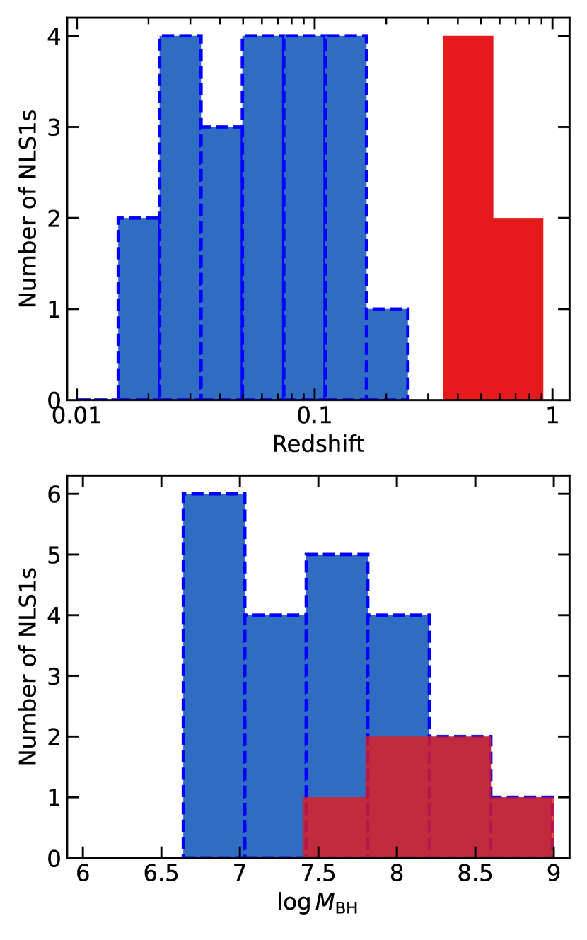
We select six NLS1s with redshift observed by the European Space Agency’s XMM-Newton satellite (Jansen et al., 2001). Details about the observations are summarized in Table 1. Their redshift and BH mass distributions are shown in Figure 1. The studied redshift range is extended much beyond the one in the previous sample. The BH masses are distributed at the upper end of the previous sample, which are estimated by the Reverberation Mapping (RM) method or the emission-line properties (see the notes in the Table for details). In addition, we include the FWHM(H) and Fe ii/H ratios from the literature in Table 2. We also show the full list of our candidate samples with their EPIC-pn count rates in Appendix A. We do not aim to conduct a thorough study of the entire population of NLS1s at the given redshift range. Instead, we want to examine how these selected NLS1s behave given their higher redshift and the at the upper end of the local sample. Future systematic studies of the NLS1s at higher redshift can be carried out with archived XMM-Newton data of NLS1 in catalogs (e.g., Rakshit & Stalin, 2017)
We use the European Photon Imaging Camera (EPIC) observations collected by EPIC-pn and EPIC-MOS (Strüder et al., 2001; Turner et al., 2001). Note that SDSS J020435 only has available EPIC-MOS data; 1WGA J2223 only has available EPIC-pn data. Both sources fall into the gaps of the CCD chips in the FoV of either EPIC-pn or EPIC-MOS. We use the XMM-Newton Science Analysis System (SAS) v20.0.0 software package to reduce the data. We first generate the clean event files using epproc (emproc) for EPIC-pn observations (EPIC-MOS observations). We then extract the good time intervals (GTIs) by selecting the time intervals with weak flaring particle backgrounds. For PG 1543+489, due to strong background flaring in all observations, we apply the iterative 3 cleaning procedure for the EPIC keV range described in Vignali et al. (2008). For other observations, we use the standard EPIC data reduction thread, where we select the single event (PATTERN=0) count rate in the keV band that is smaller than 0.40 (0.35 ) for EPIC-pn (EPIC-MOS) data. Then we filter the event lists for all observations by selecting single and double events for EPIC-pn (PATTERN4) and EPIC-MOS (PATTERN12) in a circular region. No pile-up issue is found in our observations. The backgrounds are extracted in nearby regions on the same chip. The redistribution matrix files and ancillary response files are generated by rmfgen and arfgen.
We use EPIC spectra in the keV energy range in our analysis. Given the redshift range of our sample, the analyzed rest-frame energy band is consistent with the GW+20 local samples which were analyzed in the keV band. The lightcurves of our samples do not show strong X-ray variability. For PG 1543+489, we use the epicspeccombine tool to stack the three observations from EPIC-pn, EPIC-MOS1, and EPIC-MOS2 spectra, respectively. We group the spectra using the specgroup command so that each bin has a minimum signal-to-noise ratio (SNR) of 3 (minimum SNR of 6 for PG 1543+489) and a minimum width of of the full width half maximum resolution at the central energy of the group.
3 Spectral Analysis
We use Xspec v12.12.0 (Arnaud, 1996) and the statistics in our analysis. The Galactic hydrogen column density is calculated according to Willingale et al. (2013), which is shown in Table 1. The luminosity distance is retrieved from the NED website111https://ned.ipac.caltech.edu/, where , , and are assumed.
3.1 Soft Excess Emission
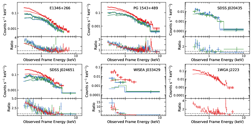
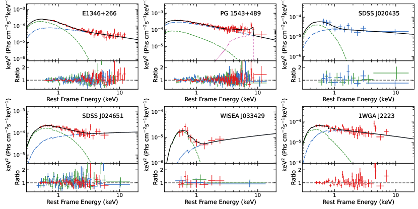
We fit the keV energy band in the observed frame with an absorbed powerlaw at the Galactic column density values ( keV for SDSS J020435 and WISEA J033429 due to inadequate data bins in the keV band). We then include the keV band data without re-fitting to illustrate the soft excess emission in our sources. We show the data/model ratio plots in Figure 2. All spectra show strong excess emission in the soft X-ray band below 1 keV. To model the soft excess component, we continue to apply a baseline model to the spectra.
3.2 Baseline Models and Eddington Ratio
We apply a phenomenological baseline model across the available energy band of keV in the observed frame. Our baseline model is
| constTBabszashift(bbody+powerlaw) |
in Xspec notation. We use powerlaw to model the high-energy Comptonized continuum, and we use the blackbody model bbody with the temperature at to fit the soft excess emission. The const is to account for the flux calibration uncertainties. The zashift model accounts for the redshift. The Tbabs model describes the absorption along the line-of-sight. As a first attempt, we allow the column density to vary. We shall show all our spectral plots in the rest frame of the sources.
The iron K emission feature around 6.4 keV is produced by the illumination of the disk by the primary X-ray source and the fluorescence of Fe K-shell electrons (Fabian et al., 1989; Miller, 2007). This feature is not prominent in our sample due to the low signal-to-noise ratio (SNR) in the iron emission band. Thus, we cannot conclude the existence of the iron K line in most objects. However, Vignali et al. (2008) found evidence of a broad iron K emission line in PG1543489, so we consider an additional component for the iron K emission for this source in our analysis by following the same approach as in Vignali et al. (2008).
For PG 1543+489, we add a relline (Dauser et al., 2010) component to model the relativistic iron K emission feature. We set the rest-frame emission line energy at as it is the best-fit value obtained by Vignali et al. (2008). The illumination pattern onto the disk, namely the emissivity profile is assumed to be a broken-powerlaw: for , and for , where is the inner emissivity index and is the breaking radius. We also allow a free BH spin and inclination angle .
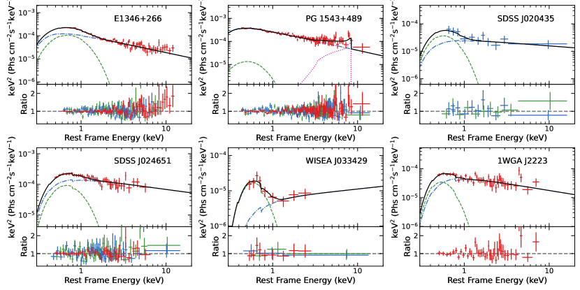
Figure 3 shows the best-fit models and data/model ratio plots for the six sources. Table 3 gives the best-fit results using the baseline models. We find that the cannot be constrained in our fits, so we fix the to the Galactic values throughout our analysis. We also report the upper limit within 90% confidence level in column (13) of Table 2. None of the sources are highly obscured. Based on the best fits, we measure the X-ray luminosity from in the rest frame after correcting for the Galactic absorption. We calculate the logarithmic Eddington ratio , where is the bolometric luminosity, with the BH mass given in Table 1. The bolometric correction factor linking the and the is estimated by the approximation in Netzer (2019):
| (1) |
We also present the measurements of by optical observations in the literature. The results are summarized in columns (7), (8), and (9) of Table 2 (see the notes therein for more information). All sources present large estimated from the X-rays except for WISEA J033429. The large Eddington ratio of our sample is consistent with the typical NLS1 behavior that they are actively accreting matter.
| (1) | (2) | (3) | (4) | (5) | (6) | (7) | (8) | (9) | (10) | (11) | (12) | (13) |
|---|---|---|---|---|---|---|---|---|---|---|---|---|
| Source | Fe ii/H | FWHM(H) | ||||||||||
| E1346+266 | 0.98 | 1840 | 0.30 | 2.16 | -1.21 | 42.5 | a | 1.6 | ||||
| PG 1543+489 | 0.86 | 1560 | 10.0 | 5.03 | -1.65 | 16.6 | b | 2.9 | ||||
| SDSS J020435 | 0.83 | 1905 | 1.40 | 0.74 | -1.64 | 8.5 | c | 29 | ||||
| SDSS J024651 | 0.49 | 1725 | 3.83 | 4.04 | -1.53 | 21 | c | 7.9 | ||||
| WISEA J033429 | 0.69 | 2127 | 3.46 | 0.23 | -1.99 | 1.4 | c | 91 | ||||
| 1WGA J2223 | — | 2000 | 1.09 | 1.21 | -1.52 | 8.3 | d | 13 |
3.3 The Soft Excess Strength: Comparison with BLS1s and NLS1s at lower redshifts
Literature shows a number of ways to quantify the soft excess strength (e.g. Piconcelli et al., 2005; Petrucci et al., 2013; Boissay et al., 2016). Here we adapt the three quantities defined in GW+20 to characterize the soft excess strength.
is defined as the ratio of the unabsorbed keV flux in the rest frame of the blackbody component over the Comptonized component:
Similarly, is the ratio of the unabsorbed rest-frame keV flux of the blackbody component over the Comptonized component:
Finally, is the ratio of the unabsorbed rest-frame keV blackbody luminosity over the Eddington luminosity:
We measure , , and using the baseline models defined in Section 3.2, where bbody is the phenomenological description of the soft excess, and the Comptonized component is modeled by powerlaw. All flux measurements are based on the model extrapolation in the rest-frame energy band. Columns (10), (11), and (12) in Table 2 summarize the measurements of the soft excess strength.
| E1346+266 | PG1543+489 | SDSS J0204 | SDSS J0246 | WISEA J033 | 1WGA J2223 | |
| bbody | ||||||
| powerlaw | ||||||
| relline | ||||||
| (keV) | ||||||
| () | ||||||
| Incl (deg) | ||||||
| 168.83/179 | 253.05/238 | 8.15/16 | 116.96/126 | 3.15/9 | 38.01/39 |
We compare the results of our sample with the NLS1s and BLS1s at lower redshift in GW+20. While their NLS1s have a median with one outlier at , our sample spans from to , which is beyond the previous sample’s range. In Figures 4, 5, and 6, the red circles are our NLS1 sample at higher redshift; the blue squares and the grey triangles are the NLS1s and BLS1s measured in GW+20. Figure 4 shows the correlations between the photon index and the . Our NLS1s roughly follow the positive trend between and as revealed by the GW+20 sample. They also show similar photon indices to the lower-redshift sources, but the is slightly lower. This comparison is band-consistent. Considering the difference in redshift, we conclude the spectra of our higher-redshift sample and the local sample in GW+20 have comparable energy ranges in the rest frame.
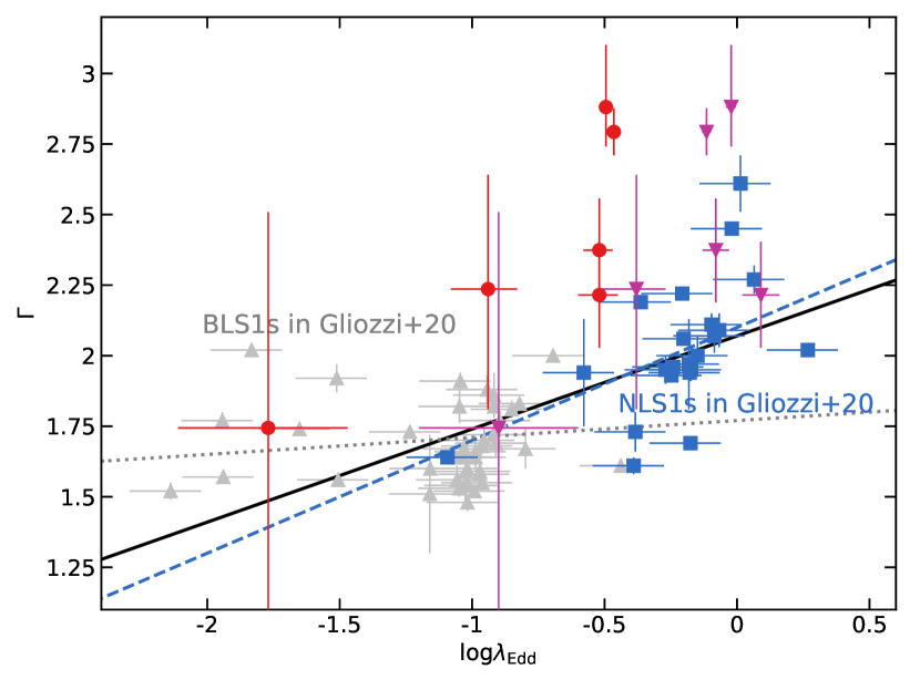
Figure 5 shows the soft excess strength versus the Eddington ratio. While the NLS1s in GW+20 show a variety of soft excess strengths, they present similar values of the Eddington ratio. This is also the case for the BLS1s in grey points. In particular, the NLS1s show relatively stronger soft excess strength than the BLS1s. Our NLS1s show a similar range of soft excess strength despite the relatively lower . Among them, WISEA J033429 presents the highest and and the second lowest . is imprinted with the absolute strength of the soft excess, as it compares the soft X-ray luminosity directly with the Eddington luminosity and thus is susceptible to the Eddington ratio. and can be a better indicator of the strength of the soft excess relative to the powerlaw continuum, regardless of the bolometric luminosity of the source.
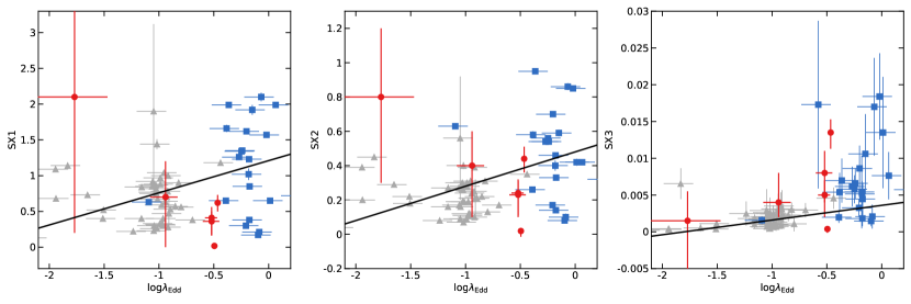
Figure 6 shows the photon index versus the soft excess strength. GW+20 presented a positive correlation in their AGN sample. Though our sources roughly follow a similar trend, we cannot be conclusive about a similar correlation due to the small number of sources. PG 1543+489 is the outlier in our sample. The soft excess strength is weak (lowest , , and in the sample), while it shows a very soft powerlaw continuum. It is also one of the most massive and luminous sources in our sample and the NLS1s in GW+20.
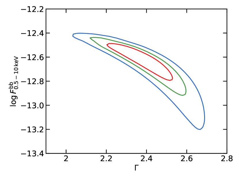
The high redshifts of our sample move a great portion of the soft excess emission beyond the lower limits of the detection range. The lack of observation above 10 keV in the observed frame also makes it hard to accurately identify the continuum. These factors would likely cause a degeneracy between the soft excess component and the powerlaw component, and thus a large uncertainty in and . To better illustrate the degeneracy, we plot the constraints on the flux of the bbody component from keV and the powerlaw photon index for SDSS J024651 in Figure 7. Although the confidence levels shown with the contours are consistent with the uncertainties in Table 3, the “banana-shaped" contours clearly show the degeneracy between the soft excess flux and the photon index. Within 99% confidence level, two possible solutions are found to explain the data with similarly good fits : (1) and (2) and .
PG1543+489 is the only source in our sample that shows a blurred iron line feature. By modeling the emission line with the relativistic line emission model relline, we would be able to probe the innermost region of the accretion disk. The results indicate a fast-spinning BH (). The emissivity profile shows a steep powerlaw () within a relatively small radius (). This scenario indicates a strong illumination from the primary source onto the innermost disk region, where the relativistic effect can play a significant role in the outgoing reflection spectrum. This is consistent with the blurred iron line feature observed in this source.
3.4 The relation
Apart from the X-ray observations, we also incorporate their historical observations at the optical and UV wavelengths. In particular, we focus on their rest-frame monochromatic luminosities and optical-to-X-ray spectral indices .
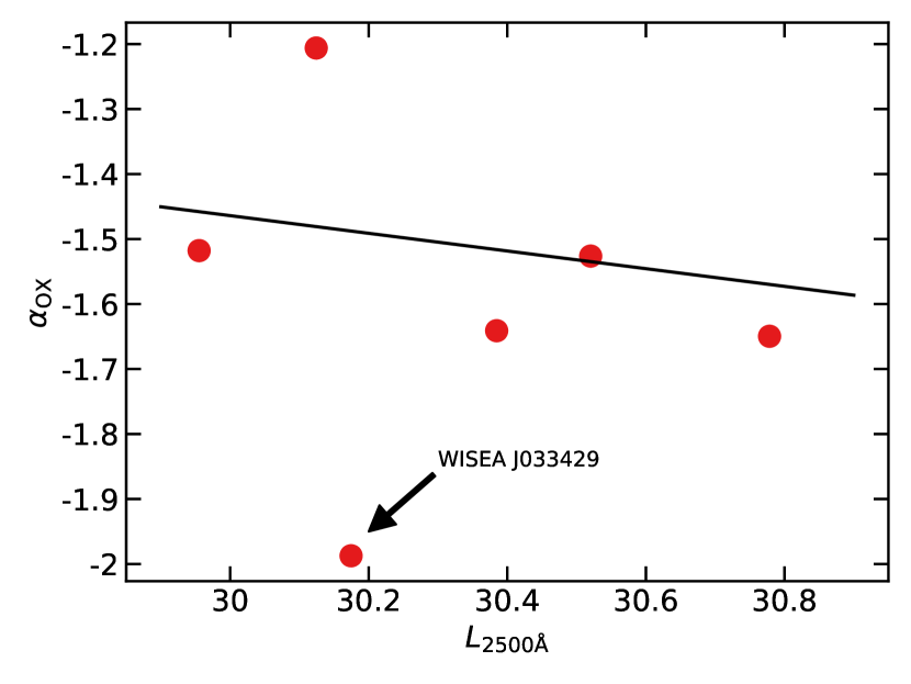
The is defined as , where and are the and rest-frame flux density; and are their corresponding frequencies. Previous studies have revealed a strong anti-correlation between and (e.g., Strateva et al., 2005; Just et al., 2007). The “simple" NLS1s defined by Gallo (2006) follow the correlation relatively well and appear to be in a typical flux state, while the “complex" NLS1 sample is representative of objects in X-ray low-flux states. They can be greatly below the nominal relation and present stronger X-ray variability.
We search the archived values and measure the according to the best-fitting baseline models of our sources. The host-galaxy contribution is not subtracted from the UV observations, introducing a level of uncertainty. The flux and the corresponding values are summarized in columns (4), (5), and (6) of Table 2. We plot the versus the in Figure 8. Most of our higher-redshift sources show good consistency with the relation of radio-quiet type 1 AGNs in Strateva et al. (2005) except for WISEA J033429. This object is significantly X-ray weak, with from the relation, corresponding to an X-ray weakness . The X-ray weakness indicates the of WISEA J033429 estimated from the X-rays is underestimated, which is consistent with the discrepancy between the X-ray and the optical Eddington ratios (; ) shown Table 2. However, as this source also shows the strongest soft excess emission relative to the continuum ( and ), the X-weakness is likely to be intrinsic. The light-bending effect in the relativistic reflection model may have an important role. In this case, most of the primary emission from the primary source is bent back toward the BH, causing an X-ray low-flux state (Ross & Fabian, 2005).
4 Discussion
4.1 Systematic Uncertainties and Selection Effects
Here we discuss the systematic effects of our measurement using the baseline models. We note that the most prominent systematic effect lies in the estimation of . For a majority of the NLS1s in GW+20, were estimated as the average value obtained by the NLS1 sample in Vasudevan & Fabian (2009). The average bolometric correction factor for NLS1s in Vasudevan & Fabian (2009) is 96.4. If we apply Equation 1 to the NLS1s in GW+20, based on their rest-frame keV luminosity, the estimated should be . Thus, in GW+20 should be overestimated by a factor of , corresponding to a difference of for . If we consider this effect in the estimation of , the separation between the two samples can naturally be resolved. We test this hypothesis by applying as in GW+20 to our NLS1s at higher redshift. We plot the results in purple in Figure 4. Our NLS1s at higher redshift now have similar and with the GW+20 NLS1s at lower redshift. This suggests the estimation of can lead to large systematic uncertainties. We emphasize that it does not indicate the estimation of in Netzer (2019) is inconsistent with the one in Vasudevan & Fabian (2009). Rather, the discrepancy in is because a constant may only work for AGNs with a relatively low (Vasudevan & Fabian, 2009). As our sources show large (), we prefer an increasing as the measured X-ray luminosities increase, as shown in Equation 1. GW+20 did not consider the dependence of on , and they did not exclude the outliers in the NLS1 samples of Vasudevan & Fabian (2009), which can lead to a highly overestimated average .
Another systematic effect results from the instrumental selection. Our sources have higher redshift, so they need higher absolute luminosity to be detected. On the other hand, they also show larger BH masses, which means they can be more luminous even with a similar . This is consistent with the results in Figure 4 after considering the systematic effect on .
A discrepancy in the methods between this work and GW+20 is that GW+20 applied the bulk-motion Comptonization model bmc to model the continuum (Shrader & Titarchuk, 1999), rather than the powerlaw model we use here. The bmc model includes four parameters: the seed photon temperature , the spectral index , the Comptonization parameter , and the normalization. We test the bmc model by fixing keV and allow other parameters to vary. The bmc model provides almost the same best-fit results, and the difference of compared with our baseline models is less than 0.02, much smaller than the discrepancy detected in Figure 4. We thus consider the discrepancy in the baseline models to be negligible.
So far we find that all our sources have significant soft excess despite that they have slightly lower or similar at higher redshift. We also apply a phenomenological model to quantify the soft excess. Now we want to use more physical models to discuss the origin of the soft excess.
4.2 The Warm Corona Model
In this section, we discuss the possibility of the warm corona model as the origin of the soft excess emission of our sources (Magdziarz et al., 1998; Petrucci et al., 2018). Under this hypothesis, the seed UV photons are up-scattered by a warm and optically thick corona. The soft excess is the high-energy tail of the Comptonized component. To do so, we replace the bbody component in our baseline models with the nthcomp model (Życki et al., 1999) to provide a more physical description of the soft excess. The nthcomp model describes the thermally Comptonized continuum produced in the warm corona. The model considers disk multi-temperature blackbody emission with seed photon temperature at as the seed spectrum. We fix as we only analyze the spectra in the X-ray band. The produced continuum can be easily controlled by the warm corona temperature and the asymptotic powerlaw photon index . The powerlaw continuum is also replaced by the cutoffpl model with the high-energy cutoff fixed at 300 keV (we replace the powerlaw model with the cutoffpl model because we want to have a consistent model setup with Section 4.3; see the description therein). As is unconstrained in our baseline models, we fix the to Galactic values. The full model in Xspec is
For PG 1543+489, we still add a relline component to model the iron K line feature. We assume a broken-powerlaw emissivity profile with variable and with at , which is the same as the treatment in the baseline model. We fix the line energy in the rest frame at . Other free parameters in the relline model are the spin (), and the inclination angle. The inner radius of the disk is assumed to reach the innermost stable circular orbit ().
Figure 9 shows the best-fit models and data/model ratio plots for the warm corona scenario. The best-fit results are summarized in Table 4. The relline component indicates a fast-spinning BH and a steep powerlaw emissivity profile, consistent with the results where the bbody model is used for the soft excess.
| E1346+266 | PG1543+489 | SDSS J0204 | SDSS J0246 | WISEA J033 | 1WGA J2223 | |
| nthcomp | ||||||
| () | ||||||
| cutoffpl | ||||||
| relline | ||||||
| (keV) | ||||||
| () | ||||||
| Incl (deg) | ||||||
| 164.82/178 | 252.69/237 | 8.22/15 | 113.83/125 | 3.29/8 | 37.73/38 |
Our sources present a highly scattered X-ray continuum () and a warm corona emission with very low temperature and large photon index (, ). This is consistent with the sample study in Petrucci et al. (2018) where 100 observations of 22 objects were studied (see Figure 5 therein).
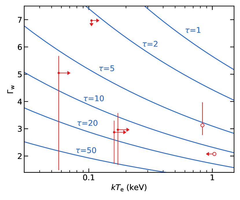
We visualize the warm corona photon index and the warm corona temperature in Figure 10, and the contours of optical depth are also plotted according to Equation (13) in Beloborodov (1999). Open circles mean either the temperature or the optical depth of the warm corona is unconstrained. We see that all sources show large except for SDSS J020435, which has an upper limit of and a lower limit of . This is in agreement with the previous studies of the warm corona in AGNs (e.g. Jin et al., 2012; Petrucci et al., 2013, 2018).
4.3 The Relativistic Disk Reflection Model
Another model commonly applied to explain the soft excess is the relativistic reflection model (Crummy et al., 2006; Fabian et al., 2009; Jiang et al., 2018b). The X-ray fluorescence emission is produced by the reprocessing of photons by the inner part of the disk. These fluorescence features will be blurred by the strong relativistic effects around the BH. This effect makes X-ray reflection spectroscopy one of the most effective tools in probing the vicinity of BH. Moreover, the existence of high-density inner-disk electrons () would further contribute to an increased emission in the soft X-ray band (Ross & Fabian, 1993; García et al., 2016).
Currently, the most advanced reflection model package is relxill (Dauser et al., 2013; García et al., 2014). It incorporates xillver, which calculates the reflection in the rest-frame of the accretion disk, and the relativistic convolution model relconv. Specifically, to model the reflection component we apply the relxillD flavor which considers a variable disk electron density () and a fixed high-energy cutoff at 300 keV. The primary effect of the high density is the increase of free-free heating in the deeper region of the disk, causing an increased disk temperature. The emission of the reflected spectrum at low energies would thus increase and may consequently resolve the existence of the soft excess (García et al., 2016; Jiang et al., 2019). The continuum is described by cutoffpl. The high-energy cutoff is also fixed at 300 keV to keep a consistent setup with the relxillD model (although the exact cutoff value is not important with our data up to in the observed frame). We fix the to Galactic values as we did in the previous analysis. The full model in Xspec notation is
Since the hard continuum is treated as the incident spectrum of the reflection component, we link the photon index of relxillD with the spectral slope of cutoffpl. For all observations, we assume a powerlaw-like disk emissivity profile . The inner radius of the disk is assumed to reach the ISCO. In a nominal fit, we allow a variable spin (), inclination angle, disk ionization (), iron abundance (), and disk density (). If neither the upper nor lower limit of can be constrained, we fix , as in the case of the standard relxill flavor. If the spin cannot be constrained, we fix . We also check that allowing a free inner disk radius would only result in a compared with a fixed . Thus, we choose to fix the at the ISCO. If there are other unconstrained parameters, we would further decrease the degrees of freedom by fixing , , and . In the end, for the least constrained fit, the only free parameters are the photon index and the ionization parameter , in addition to the normalization.
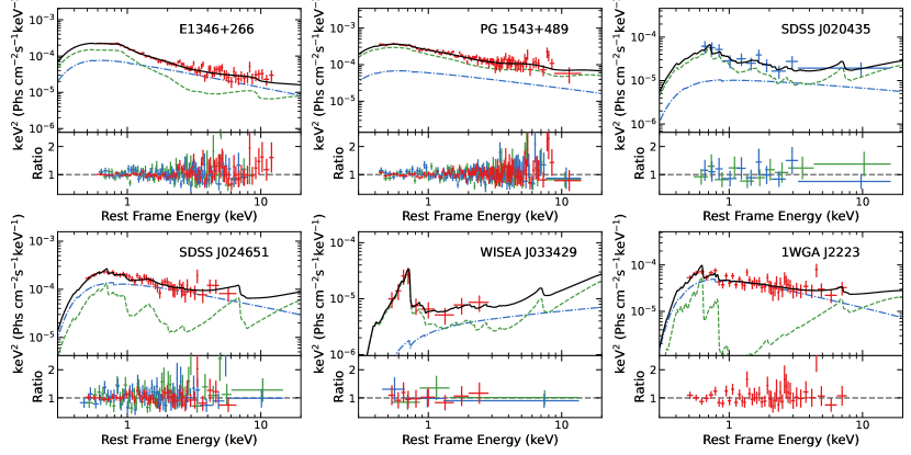
Figure 11 shows the best-fit models and data/model ratio plots for the relativistic reflection model. Table 5 summarizes the best-fit parameter values. The relativistic reflection model provides similarly good fits compared with the warm corona model. All sources show a very soft continuum with except for WISEA J033429. This source shows the most significant X-ray weakness, and it has a large uncertainty on with an upper limit value of 2.4 within 90% confidence level. The co-existence of the X-ray weakness and the strong and in this source can be explained by the relativistic reflection. The relativistic reflection blurs a series of emission lines in the soft X-ray band, causing an “excess" of emission; in the meantime, the light-bending effect causes a portion of the primary emission from the hot corona to bend towards the BH and thus results in an X-ray low-flux state. Our spectral fitting confirms a reflection-dominated spectrum in WISEA J033429 (Figure 11), which further supports the relativistic reflection. The conclusion is similar to the one in García et al. (2019), in which they studied a nearby () bright Seyfert 1 AGN Mrk 509.
| E1346+266 | PG1543+489 | SDSS J0204 | SDSS J0246 | WISEA J033 | 1WGA J2223 | |
| cutoffpl | ||||||
| relxillD | ||||||
| Incl (deg) | ||||||
| 163.83/174 | 254.95/239 | 8.37/16 | 107.09/121 | 2.71/8 | 37.61/39 |
Interestingly, our sources show slightly higher ionization than typical Sy1s (, see e.g., Walton et al., 2013). A high ionization can contribute to the soft excess together with a high-density disk. The BH spins of these sources are also not well constrained due to a low SNR in the iron band. The most stringent constraints come from E1346+266 and PG 1543+489. Both sources indicate a rapidly spinning BH ( and , respectively).
According to the standard -disk model by Shakura & Sunyaev (1973), Svensson & Zdziarski (1994) gave a relationship between the density of a radiation-pressure-dominated disk at radius and the accretion rate
| (2) |
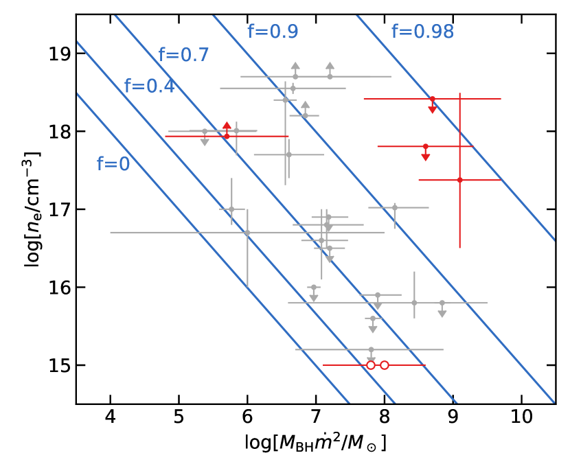
where is the Thompson cross section, is the Schwarzchild radius, and is the radius on the disk in units of . We take as the standard viscosity parameter (Shakura & Sunyaev, 1973), and in the radiative diffusion equation, and is the fraction of the total transported accretion power released from the disk to the hot corona (Xu et al., 2021). The dimensionless accretion rate is defined as , where is the efficiency for converting accreted mass into outgoing radiation. for a Schwarzschild BH () and for a maximally spinning Kerr BH () (Thorne, 1974). We assume in our analysis so that it takes into account all possible values of , and we propagate the uncertainties to the estimated accretion rates of our sample. According to Equation 2, . Figure 12 shows versus . The solid lines show the analytic solution for different values of assuming . The red points are the high- sources in our sample, and the grey points are the samples studied in Jiang et al. (2019). The open circles indicate that the results cannot be constrained. Taking into account the uncertainties in , our sources roughly follow the trend as predicted in Svensson & Zdziarski (1994) that a system with lower tends to have higher . The only source with constrained measurements of is E1346+266, which has the largest mass and highest redshift among our sources. In this source, about 95% of the energy in the disk is released to the corona, and the radiation-pressure dominated region is to explain the inferred high disk density.
5 Conclusion
We performed a detailed spectral analysis of six NLS1s at using XMM-Newton EPIC data. Our samples show large BH masses at the upper end of the local samples () and slightly lower or similar . We discover that all these sources have strong soft excess emission below 2 keV with relatively soft continuum.
After confirming the existence of the soft excess emission, we use the phenomenological bbody model to quantify the soft excess strength and compare the results from our higher-redshift sample with the local NLS1s and BLS1s in GW+20. We find that the soft excess strength does not show much deviation from the previous sample. We also obtain the relation and find the most X-ray-weak source WISEA J033429 is intrinsically X-ray weak judging from its strong and . We discuss in detail the impact of the bolometric correction factor , and conclude it carries the major systematic uncertainties in our measurements. The systematic difference of the estimated can explain the discrepancy of between our high-redshift sample and GW+20 sample. This further suggests the higher absolute luminosities of our sources are driven by BH mass rather than . For such detailed spectral analysis in our work, the high-redshift and the soft nature of the sources pose a great challenge for us to accurately identify the continuum, which results in a degeneracy in the parameters.
We then further consider more physical scenarios, the warm-corona model and the relativistic reflection model, to account for the soft excess. These two models provide almost equally good fits. They also allow us to probe the properties of the innermost region of the AGNs. We show that in the warm-corona scenario, the warm coronae of our sample have a low temperature () and large optical depth (); in the reflection scenario, the sources show relatively higher ionization than the samples in Walton et al. (2013). We are also able to constrain the high spin values of several sources. Combining both facts that WISEA J033429 shows the strongest relative soft excess strength with respect to the continuum emission and it shows a reflection-dominated spectrum, we tentatively conclude the relativistic reflection is a more promising explanation for the soft excess, though we cannot exclude the warm corona model based on the statistics. in the entire. Detailed tests of different models for the soft excess are better carried out with bright local samples, which is beyond the scope of this work.
The low SNR in the iron line band does not allow us to identify the iron line feature confidently. Observations from future X-ray missions like Athena may be able to provide better constraints on the spectral shape. The large effective area and energy resolution in the iron line band would allow us to better model the reflection spectrum and might help determine the contribution to the soft excess (Parker et al., 2022).
While both the warm-corona and relativistic reflection are possible explanations for the soft excess, it is natural to consider reflection from the disk in addition to Comptonization in a warm corona (Xu et al., 2021). Recently, Xiang et al. (2022) used a new model reXcor that self-consistently combines a warm corona and ionized reflection, and analyzes two Seyfert galaxies HE 1131-1820 and NGC 4593. Although the geometry of the systems is much simplified, the model was able to produce several broadened reflection features with a variety of shapes of the soft excess. Such a type of model may provide new insights about the NLS1s at higher redshift.
Acknowledgements
Z.Y. thanks Mario Gliozzi for sharing the data in GW+20 and acknowledges support from the Verne M. Willaman Distinguished Graduate Fellowships in Science. J.J. acknowledges support from the Leverhulme Trust, the Isaac Newton Trust, and St Edmund’s College.
Data Availability
The data underlying this article are available in the High Energy Astrophysics Science Archive Research Center (HEASARC), at https://heasarc.gsfc.nasa.gov. The relxill package can be downloaded at http://www.sternwarte.uni-erlangen.de/~dauser/research/relxill/.
References
- Alston et al. (2020) Alston W. N., et al., 2020, Nature Astronomy, 4, 597
- Arnaud (1996) Arnaud K. A., 1996, in Jacoby G. H., Barnes J., eds, Astronomical Society of the Pacific Conference Series Vol. 101, Astronomical Data Analysis Software and Systems V. p. 17
- Bambi et al. (2021) Bambi C., et al., 2021, Space Sci. Rev., 217, 65
- Baskin & Laor (2004) Baskin A., Laor A., 2004, MNRAS, 350, L31
- Beloborodov (1999) Beloborodov A. M., 1999, in Poutanen J., Svensson R., eds, Astronomical Society of the Pacific Conference Series Vol. 161, High Energy Processes in Accreting Black Holes. p. 295 (arXiv:astro-ph/9901108)
- Bianchi et al. (2009) Bianchi S., Guainazzi M., Matt G., Fonseca Bonilla N., Ponti G., 2009, A&A, 495, 421
- Boissay et al. (2016) Boissay R., Ricci C., Paltani S., 2016, A&A, 588, A70
- Boller et al. (1996) Boller T., Brandt W. N., Fink H., 1996, A&A, 305, 53
- Boroson (2002) Boroson T. A., 2002, ApJ, 565, 78
- Boroson & Green (1992) Boroson T. A., Green R. F., 1992, ApJS, 80, 109
- Crummy et al. (2006) Crummy J., Fabian A. C., Gallo L., Ross R. R., 2006, MNRAS, 365, 1067
- Dauser et al. (2010) Dauser T., Wilms J., Reynolds C. S., Brenneman L. W., 2010, MNRAS, 409, 1534
- Dauser et al. (2013) Dauser T., Garcia J., Wilms J., Böck M., Brenneman L. W., Falanga M., Fukumura K., Reynolds C. S., 2013, MNRAS, 430, 1694
- Fabian et al. (1989) Fabian A. C., Rees M. J., Stella L., White N. E., 1989, MNRAS, 238, 729
- Fabian et al. (2002) Fabian A. C., Ballantyne D. R., Merloni A., Vaughan S., Iwasawa K., Boller T., 2002, MNRAS, 331, L35
- Fabian et al. (2009) Fabian A. C., et al., 2009, Nature, 459, 540
- Fabian et al. (2015) Fabian A. C., Lohfink A., Kara E., Parker M. L., Vasudevan R., Reynolds C. S., 2015, MNRAS, 451, 4375
- Frank et al. (2002) Frank J., King A., Raine D. J., 2002, Accretion Power in Astrophysics: Third Edition
- Gallo (2006) Gallo L. C., 2006, MNRAS, 368, 479
- Gallo (2018) Gallo L., 2018, in Revisiting Narrow-Line Seyfert 1 Galaxies and their Place in the Universe. p. 34 (arXiv:1807.09838)
- García et al. (2014) García J., et al., 2014, ApJ, 782, 76
- García et al. (2016) García J. A., Fabian A. C., Kallman T. R., Dauser T., Parker M. L., McClintock J. E., Steiner J. F., Wilms J., 2016, MNRAS, 462, 751
- García et al. (2019) García J. A., et al., 2019, ApJ, 871, 88
- Gliozzi & Williams (2020) Gliozzi M., Williams J. K., 2020, MNRAS, 491, 532
- Goodrich (1989) Goodrich R. W., 1989, ApJ, 342, 224
- Grandi et al. (2004) Grandi P., Foschini L., Masetti N., Palazzi E., 2004, A&A, 418, 907
- Grupe (2004) Grupe D., 2004, AJ, 127, 1799
- Grupe & Mathur (2004) Grupe D., Mathur S., 2004, ApJ, 606, L41
- Grupe et al. (1999) Grupe D., Beuermann K., Mannheim K., Thomas H. C., 1999, A&A, 350, 805
- Grupe et al. (2001) Grupe D., Thomas H. C., Beuermann K., 2001, A&A, 367, 470
- Haardt & Maraschi (1991) Haardt F., Maraschi L., 1991, ApJ, 380, L51
- Jansen et al. (2001) Jansen F., et al., 2001, A&A, 365, L1
- Jiang et al. (2018a) Jiang J., et al., 2018a, MNRAS, 477, 3711
- Jiang et al. (2018b) Jiang J., et al., 2018b, MNRAS, 477, 3711
- Jiang et al. (2019) Jiang J., et al., 2019, MNRAS, 489, 3436
- Jiang et al. (2020) Jiang J., Gallo L. C., Fabian A. C., Parker M. L., Reynolds C. S., 2020, MNRAS, 498, 3888
- Jin et al. (2009) Jin C., Done C., Ward M., Gierliński M., Mullaney J., 2009, MNRAS, 398, L16
- Jin et al. (2012) Jin C., Ward M., Done C., Gelbord J., 2012, MNRAS, 420, 1825
- Just et al. (2007) Just D. W., Brandt W. N., Shemmer O., Steffen A. T., Schneider D. P., Chartas G., Garmire G. P., 2007, ApJ, 665, 1004
- Karttunen et al. (2007) Karttunen H., Kröger P., Oja H., Poutanen M., Donner K. J., 2007, Fundamental astronomy. Springer
- Kaspi et al. (2000) Kaspi S., Smith P. S., Netzer H., Maoz D., Jannuzi B. T., Giveon U., 2000, ApJ, 533, 631
- Kelly et al. (2008) Kelly B. C., Bechtold J., Trump J. R., Vestergaard M., Siemiginowska A., 2008, ApJS, 176, 355
- Laor (2019) Laor A., 2019, Nature Astronomy, 3, 374
- Leighly (1999) Leighly K. M., 1999, ApJS, 125, 297
- Magdziarz et al. (1998) Magdziarz P., Blaes O. M., Zdziarski A. A., Johnson W. N., Smith D. A., 1998, MNRAS, 301, 179
- Marinucci et al. (2014) Marinucci A., et al., 2014, ApJ, 787, 83
- Markoff et al. (2005) Markoff S., Nowak M. A., Wilms J., 2005, ApJ, 635, 1203
- Middleton et al. (2007a) Middleton M., Done C., Gierliński M., 2007a, MNRAS, 381, 1426
- Middleton et al. (2007b) Middleton M., Done C., Gierliński M., 2007b, MNRAS, 381, 1426
- Miller (2007) Miller J. M., 2007, ARA&A, 45, 441
- Miller et al. (2002) Miller J. M., et al., 2002, ApJ, 570, L69
- Miniutti & Fabian (2004) Miniutti G., Fabian A. C., 2004, MNRAS, 349, 1435
- Netzer (2019) Netzer H., 2019, MNRAS, 488, 5185
- Osterbrock & Dahari (1983) Osterbrock D. E., Dahari O., 1983, ApJ, 273, 478
- Osterbrock & Pogge (1985) Osterbrock D. E., Pogge R. W., 1985, ApJ, 297, 166
- Parker et al. (2014) Parker M. L., et al., 2014, MNRAS, 443, 1723
- Parker et al. (2018) Parker M. L., Miller J. M., Fabian A. C., 2018, MNRAS, 474, 1538
- Parker et al. (2022) Parker M. L., Matzeu G. A., Matthews J. H., Middleton M. J., Dauser T., Jiang J., Joyce A. M., 2022, MNRAS, 513, 551
- Peterson (1997) Peterson B. M., 1997, An introduction to active galactic nuclei. Cambridge University Press
- Petrucci et al. (2013) Petrucci P. O., et al., 2013, A&A, 549, A73
- Petrucci et al. (2018) Petrucci P. O., Ursini F., De Rosa A., Bianchi S., Cappi M., Matt G., Dadina M., Malzac J., 2018, A&A, 611, A59
- Piconcelli et al. (2005) Piconcelli E., Jimenez-Bailón E., Guainazzi M., Schartel N., Rodríguez-Pascual P. M., Santos-Lleó M., 2005, A&A, 432, 15
- Rakshit & Stalin (2017) Rakshit S., Stalin C. S., 2017, ApJ, 842, 96
- Rakshit et al. (2017) Rakshit S., Stalin C. S., Chand H., Zhang X.-G., 2017, ApJS, 229, 39
- Reynolds (2021) Reynolds C. S., 2021, ARA&A, 59, 117
- Reynolds & Nowak (2003) Reynolds C. S., Nowak M. A., 2003, Phys. Rep., 377, 389
- Ross & Fabian (1993) Ross R. R., Fabian A. C., 1993, MNRAS, 261, 74
- Ross & Fabian (2005) Ross R. R., Fabian A. C., 2005, MNRAS, 358, 211
- Shakura & Sunyaev (1973) Shakura N. I., Sunyaev R. A., 1973, A&A, 24, 337
- Shen et al. (2011) Shen Y., et al., 2011, ApJS, 194, 45
- Shrader & Titarchuk (1999) Shrader C. R., Titarchuk L., 1999, ApJ, 521, L121
- Sisk-Reynés et al. (2022) Sisk-Reynés J., Reynolds C. S., Matthews J. H., Smith R. N., 2022, MNRAS, 514, 2568
- Strateva et al. (2005) Strateva I. V., Brandt W. N., Schneider D. P., Vanden Berk D. G., Vignali C., 2005, AJ, 130, 387
- Strüder et al. (2001) Strüder L., et al., 2001, A&A, 365, L18
- Svensson & Zdziarski (1994) Svensson R., Zdziarski A. A., 1994, ApJ, 436, 599
- Tanaka et al. (2004) Tanaka Y., Boller T., Gallo L., Keil R., Ueda Y., 2004, PASJ, 56, L9
- Thorne (1974) Thorne K. S., 1974, ApJ, 191, 507
- Turner et al. (2001) Turner M. J. L., et al., 2001, A&A, 365, L27
- Vasudevan & Fabian (2009) Vasudevan R. V., Fabian A. C., 2009, MNRAS, 392, 1124
- Vignali et al. (2008) Vignali C., Piconcelli E., Bianchi S., Miniutti G., 2008, MNRAS, 388, 761
- Waddell & Gallo (2020) Waddell S. G. H., Gallo L. C., 2020, MNRAS, 498, 5207
- Walton et al. (2013) Walton D. J., Nardini E., Fabian A. C., Gallo L. C., Reis R. C., 2013, MNRAS, 428, 2901
- Wang et al. (2009) Wang J.-G., et al., 2009, ApJ, 707, 1334
- Wilkins & Fabian (2012) Wilkins D. R., Fabian A. C., 2012, MNRAS, 424, 1284
- Willingale et al. (2013) Willingale R., Starling R. L. C., Beardmore A. P., Tanvir N. R., O’Brien P. T., 2013, MNRAS, 431, 394
- Xiang et al. (2022) Xiang X., et al., 2022, arXiv e-prints, p. arXiv:2206.06825
- Xu et al. (2021) Xu Y., García J. A., Walton D. J., Connors R. M. T., Madsen K., Harrison F. A., 2021, ApJ, 913, 13
- Yuan et al. (2007) Yuan W., et al., 2007, in Ho L. C., Wang J. W., eds, Astronomical Society of the Pacific Conference Series Vol. 373, The Central Engine of Active Galactic Nuclei. p. 529 (arXiv:astro-ph/0612470)
- Życki et al. (1999) Życki P. T., Done C., Smith D. A., 1999, MNRAS, 309, 561
Appendix A Candidate NLS1 Sample
Here we present a list of candidate sources we have examined before our analysis in Table 6. These sources are identified as NLS1s in the optical bands. We examine their X-ray visibility in the XMM-Newton archive. We include the six sources with the highest count rates () in our analysis.
| Full Name | XMM-Newton | EPIC-pn count rate | |
|---|---|---|---|
| ObsID | upper limit (cts/s) | ||
| E1346+266 | 0.92 | 0109070201 | 0.310 |
| PG 1543+489 | 0.40 | 0153220401 | |
| 0505050201 | 0.512 (stacked) | ||
| 0505050701 | |||
| SDSS J014123.32000752.8 | 0.97 | 0747430101 | 0.019 |
| SDSS J020435.18093154.9 | 0.62 | 0763910301 | 0.061 |
| SDSS J024651.91005930.9 | 0.47 | 0402320101 | 0.369 |
| SDSS J150728.65523137.6 | 0.85 | 0804620201 | 0.005 |
| WISEA J033429.44000610.9 | 0.35 | 0402320201 | 0.021 |
| 1WGA J2223.70206 | 0.46 | 0090050601 | 0.097 |