Detecting Novelties with Empty Classes

Abstract

For open world applications, deep neural networks (DNNs) need to be aware of previously unseen data and adaptable to evolving environments. Furthermore, it is desirable to detect and learn novel classes which are not included in the DNNs underlying set of semantic classes in an unsupervised fashion. The method proposed in this article builds upon anomaly detection to retrieve out-of-distribution (OoD) data as candidates for new classes. We thereafter extend the DNN by $k$ empty classes and fine-tune it on the OoD data samples. To this end, we introduce two loss functions, which 1) entice the DNN to assign OoD samples to the empty classes and 2) to minimize the inner-class feature distances between them. Thus, instead of ground truth which contains labels for the different novel classes, the DNN obtains a single OoD label together with a distance matrix, which is computed in advance. We perform several experiments for image classification and semantic segmentation, which demonstrate that a DNN can extend its own semantic space by multiple classes without having access to ground truth.

1 Introduction

(a) image

(b) ground truth

(c) baseline

(d) ours

Figure 1: Comparison of two segmentation DNNs which were extended by the classes human and car. While the segmentation masks are similar for the initial classes, the humans and cars are much better segmented by the DNN which was extended by our empty classes approach. The novel classes are marked with green contours in the image and ground truth.

For computer vision tasks such as image classification or semantic segmentation, deep neural networks (DNNs) learn to classify instances, either on a per image- or per pixel-level, into a limited number of predefined classes. State-of-the-art DNNs achieve high accuracy when trained in a supervised fashion and deployed in a closed world setting, in which the learner is not confronted with out-of-distribution (OoD) data. In practice, however, concepts not seen at training time might occur, which is why so-called open world recognition [1] has emerged as a practically more relevant problem formulation. It combines OoD detection with class-incremental learning, i.e. , retraining the model with newly observed classes. Nevertheless, methods of this kind are typically updated in a supervised fashion, commonly employing humans for annotation.

First attempts to learn in an unsupervised manner have been made to achieve cheaper labeling. In open world image classification, clustering methods like k-means [25] or DBSCAN [13] allow for an unsupervised labeling of instances in feature regions that appear to be novel. Approaches in this direction leverage such methods to obtain pseudo labels for detected OoD images [17, 37].

However, the quality of these pseudo labels strongly depends on the clustering performance. Furthermore, the OoD candidates are assigned to fixed labels, which are likely to be noisy and thus unreliable, whereas in our method, they are put in relation to each other. In open world semantic segmentation [39, 29], pseudo labeling on a per pixel-level is required, rendering the problem more complex. More recently, few-shot learning [5], where a model is trained to generalize well on novel classes with only few labeled examples, has also been proposed to deal with the lack of labeled data as another (semi-)supervised strategy.

Figure 2: (I) A binary classification model is trained on two classes and additional noise data for entropy maximization. (II) OoD samples in the test data are obtained by entropy thresholding. (III) The training data is enriched with the OoD samples and a distance matrix, containing their pair-wise Euclidean distances. (IV) The model is class-incrementally extended by three novel classes.

In our work, we introduce a new unsupervised approach for incrementally extending DNNs by capturing novel concepts in additional classes of hypothetical nature. To this end, we proceed from an initial model aware of hitherto known classes, which is augmented by an out-of-distribution detection mechanism to distinguish these classes from unknown categories. When treating additional data with potentially additional but unknown classes, we suggest to extend the model by additional auxiliary neurons in the DNN’s output layer constituting the suspected novel classes to be recognized, which we dub empty classes. To predict outcomes of these classes, our model is fine-tuned by a clustering loss that aims to recognize similar concepts for out-of-distribution data, allowing to flexibly adapt the learned feature representations to distinguish the already known classes from the new learning outcomes.

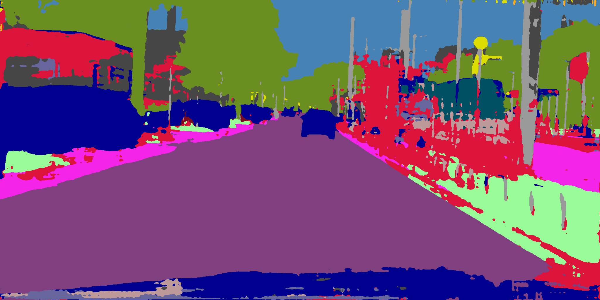
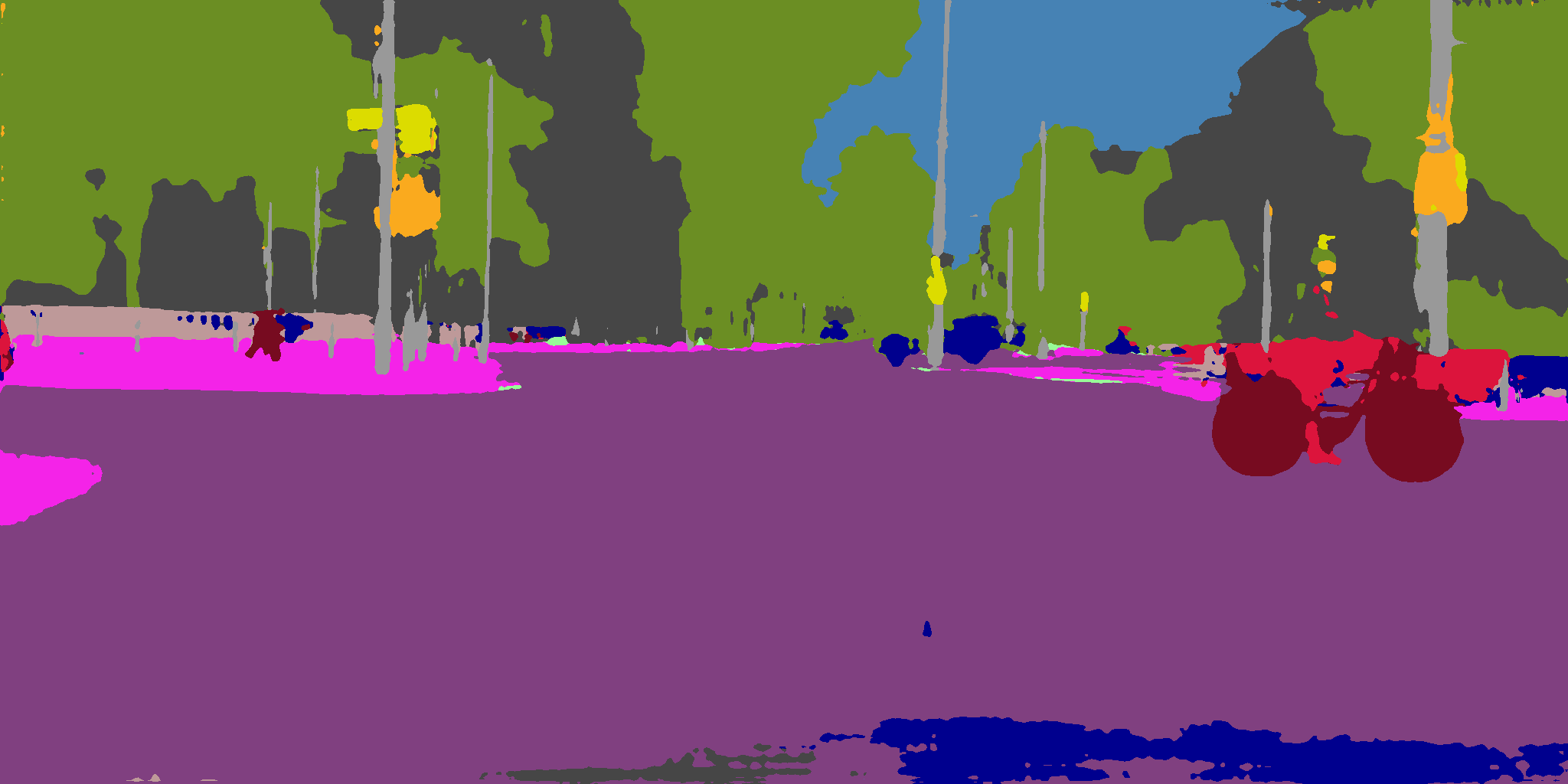
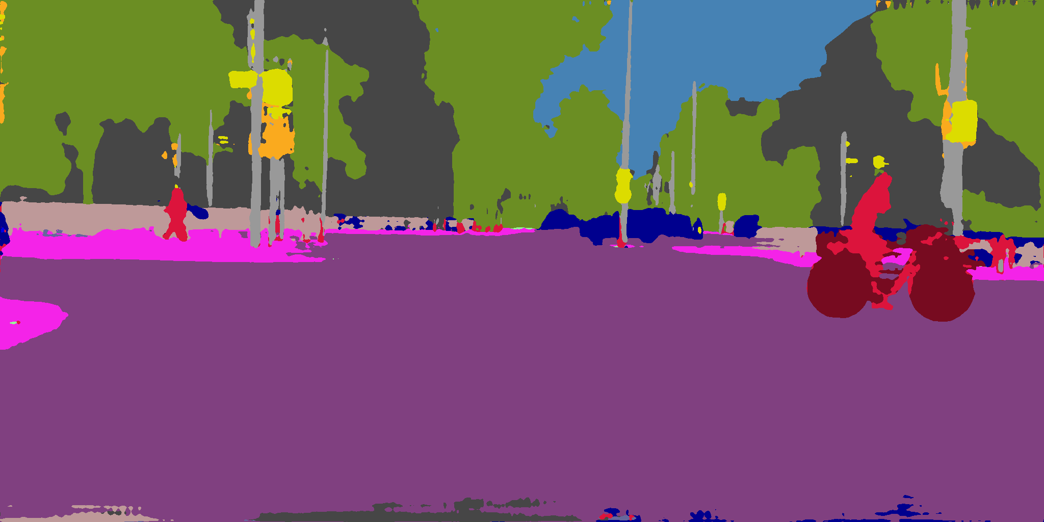
We conduct experiments on several datasets with increasing level of difficulty, starting with image classification of MNIST [21] digits as well as the slightly more sophisticated data from FashionMNIST [42]. Next, we apply our approach to low- and medium-resolution images from the CIFAR10 [20] and Animals10 dataset, respectively. Finally, we also adapt our method to the complex task of semantic segmentation of street scenes from the Cityscapes [11] dataset. In three out of four image classification experiments, our method outperforms the baseline, where a DNN is fine-tuned on $k$-means labeled OoD data. Furthermore, our extended segmentation DNN achieves better results than the baseline [39] for the novel class car, and significantly reduces the number of overlooked humans. See Fig. 1 for an example.

2 Related Work

Open world recognition [1] refers to the problem of adapting a learning system to a non-delimitable and potentially constantly evolving target domain. As such, it combines the disciplines of open set learning [35], where incomplete knowledge over the target domain is assumed at training time, with incremental learning [4], in which the model is updated by exploring additional target space regions at test time, thereby adapting to novel target information. Typically, open set recognition is formalized by specifying a novelty detector, a labeling process and an incremental learning function, allowing for a generalized characterization of such systems [1].

Most of previous approaches consider the open world recognition problem in the context of classification, where novel concepts are in form of previously unseen classes. While a plethora of methods has been proposed to tackle the individual sub-problems for classification problems, for which we refer to [31] for a more comprehensive overview, literature on holistic approaches for open world classification is rather scarce. In [37], a metric learning approach is used to distinguish between pairs of instances belonging to the same classes, allowing to detect instances that can not be mapped to known classes and being used to learn novel class concepts. Moreover, [30] suggests a semi-supervised learning approach that applies clustering on learned feature representations to reason about unknown classes. Related to this, [40] describes a kernel method using an alternative loss formulation to learn embeddings to be clustered for class discovery. More recently, similar concepts have also been tailored to specific data modalities, such as tabular data [38].

In the domain of semantic segmentation, open world recognition is also covered under the term zero-shot semantic segmentation [2]. To predict unseen categories for classified pixels, a wide range of methods leverage additional language-based context information [2, 41, 24]. Besides enriching visual information by text, unsupervised methods, e.g. , employing clustering based on visual similarity [39] or contrastive losses [14, 6], have also been considered. More recently, [7] adopts semantic segmentation based on LiDAR point clouds by augmenting conventional classifiers with predictors recognizing unknown classes, thereby enabling incremental learning.

In a more general context, unsupervised representation learning [32] constitutes a major challenge to generalize learning methods to unseen concepts. Methods of this kind are typically tailored to data modalities, e.g. , by specifying auxiliary tasks to be solved [15, 43]. In the domain of images, self-supervised learning approaches have emerged recently [3, 22], which commonly apply knowledge distillation between different networks, allowing for learning in a self-supervised fashion. Other methods including ideas stemming from metric [16] or contrastive learning [10].

Figure 3: Open world recognition models must be able to recognize known classes while detecting OoD data from novel classes and furthermore to incrementally learn these novel classes. Instead of labeling the OoD samples, our method computes pair-wise distances between them, which serve as input for a clustering loss function.

3 Method Description

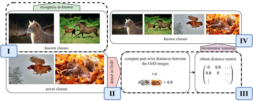
In this section, we present our training framework for unsupervised class-incremental learning with empty classes. For the sake of brevity, all equations are introduced for image classification and adapted to semantic segmentation in Sec. 4. First, we give a motivating example in Fig. 2, where we enrich data stemming from the TwoMoons dataset with OoD samples and extend the model by three novel classes. Details on this experiment are provided in the appendix. The following method description is also illustrated in Fig. 3.

I) Learning Model

For an input image $x\in\mathcal{X}$, let $f(x)\in(0,1)^{q}$ denote the softmax probabilities of some image classification model $f:\mathcal{X}\to(0,1)^{q}$ with underlying classes $\mathcal{C}=\{1,\ldots,q\}$. Consider a test dataset which includes images from classes $c\in\{1,\ldots,q,q+1,\ldots\}$. Note that our framework does not necessarily assume labels for the test data as these will be only used for evaluation and not during the training. Furthermore, let $u(f(x))\in[0,1]$ denote some arbitrary uncertainty score which derives from the predicted class-probabilities $f(x)$. Thus, a test image $x$ is considered to be OoD, if $u(f(x))>\tau$ for some threshold $\tau\in[0,1]$.

Next, we extend the initial model $f$ by $k\in\mathbb{N}$ empty classes in the final classification layer, which is then denoted as $f^{k}:\mathcal{X}\to(0,1)^{q+k}$, and fine-tune it on the OoD data $\mathcal{X}^{\mathrm{OoD}}$. Therefore, we compute pairwise distances $d_{ij}=d(x_{i},x_{j})$ for all $(x_{i},x_{j})\in\mathcal{X}^{\mathrm{OoD}}\times\mathcal{X}^{\mathrm{OoD}}$ as a pre-processing step, e.g.  using the pixel-wise Euclidean distance or any distance metric in the feature space of some embedding network. The model $f^{k}$ is then fine-tuned on (a subset of) the initial training data $\mathcal{X}^{\mathrm{train}}$, enriched with the OoD samples from the test data. For the in-distribution samples $(x,y)$, we compute the cross-entropy loss

$$\ell_{\mathrm{ce}}(x,y)=-\sum_{c=1}^{q}\mathbbm{1}_{\{c=y\}}\log(f^{k}_{c}(x))\;.$$ (1)

Further, we entice the model to predict one of the empty classes $q+1,\ldots,q+k$ for OoD data by minimizing the class-probabilities $f^{k}_{1}(x),\ldots,f^{k}_{q}(x)$, $x\in\mathcal{X}^{\mathrm{OoD}}$, i.e. , by computing

$$\ell_{\mathrm{ext}}(x)=\frac{1}{q}\sum_{c=1}^{q}f^{k}_{c}(x)\;.$$ (2)

Finally, we aim to divide the data among the empty classes based on their similarity. Thus, our clustering loss is computed pair-wise as

$$\ell_{\mathrm{cluster}}(x_{i},x_{j})=\frac{\alpha}{q+k}\cdot d_{ij}\cdot\sum_{c=1}^{q+k}f^{k}_{c}(x_{i})f^{k}_{c}(x_{j})\;,$$ (3)

where $\alpha\in\mathbb{R}_{>0}$ can be adjusted to control the impact of the clustering loss function. Together, these three loss functions give the overall objective

$$L =\lambda_{1}\mathbb{E}_{(x,y)\sim\mathcal{X}^{\mathrm{train}}}[\ell_{\mathrm{ce}}(x,y)]$$

$$+\lambda_{2}\mathbb{E}_{x\sim\mathcal{X}^{\mathrm{OoD}}}[\ell_{\mathrm{ext}}(x)]$$ (4)

$$+\lambda_{3}\mathbb{E}_{x_{i},x_{j}\sim\mathcal{X}^{\mathrm{OoD}}}[\ell_{\mathrm{cluster}}(x_{i},x_{j})]\;,$$

where the hyperparameters $\lambda_{1}$, $\lambda_{2}$ and $\lambda_{3}$ can be adjusted to balance the impact of the objectives.

II) OoD Detection

OoD detection is a pre-processing part of our framework, which can be exchanged in a plug and play manner. In our experiments, we implemented entropy maximization [18] for image classification and thus perform OoD detection by thresholding on the softmax entropy.

The idea of entropy maximization is the inclusion of known unknowns into the training data of the initial model in order to entice it to exhibit a high softmax entropy

$$u(x)=-\frac{1}{\log(q)}\sum_{c=1}^{q}f_{c}(x)\log(f_{c}(x))$$ (5)

on OoD data $x\in\mathcal{X}^{\mathrm{OoD}}$. Therefore, during training the initial model, we compute the entropy maximization loss

$$\ell_{\mathrm{em}}(x)=-\sum\limits_{c=1}^{q}\frac{1}{q}\log(f_{c}(x))$$ (6)

for known unknowns $x\in\mathcal{X}^{\mathrm{OoD}}$, giving the overall objective

$$L =\lambda~{}\mathbb{E}_{(x,y)\sim\mathcal{X}^{\mathrm{train}}}[\ell_{\mathrm{ce}}(x,y)]$$

$$+(1-\lambda)~{}\mathbb{E}_{x\sim\mathcal{X}^{\mathrm{OoD}}}[\ell_{\mathrm{em}}(x)]\;.$$ (7)

In the Two Moons example, these OoD data was uniformly distributed noise. For image classification, we employ the domain-agnostic data augmentation technique mixup [44]. This is, an OoD image is obtained by computing the average of two in-distribution samples. Entropy maximization was also introduced for semantic segmentation of street scenes [19, 9], where the OoD samples originate from the COCO dataset [23]. Furthermore, the OoD loss and data was only included in the final training epochs, which means that existing networks can be fine-tuned for entropy maximization.

III) Distance Matrix

Next, we compute pair-wise distances for the detected OoD samples, which constitute the OoD dataset for the incremental learning. For simple datasets such as TwoMoons or MNIST, the distance can be measured directly between the data samples. For MNIST, this is done by flattening the images and computing the Euclidean distance between the resulting vectors. For more complex datasets, we employ embedding networks to extract useful features of the images. These embedding networks are arbitrary image classification models, trained on large datasets such as ImageNet [12] or CIFAR100 [20], which need to be chosen carefully and individually for each experiment as the clustering loss strongly depends on their ability to extract separable features for the known and especially the novel classes.

The feature distances are either computed in the high-dimensional feature space directly, or, for the sake of transparency and better visual control, in a low-dimensional re-arrangement. Applying the manifold learning technique UMAP [27] to the entire test data, we reduce the dimension of the feature space to two . The distance matrix is then computed as the Euclidean distances in the low-dimensional space for all pairs of OoD samples.

IV) Incremental Learning

For class-incremental learning, we minimize three different loss functions defined in Eqs. 1, 2 and 3. The cross-entropy loss (1) is computed for in-distribution to mitigate catastrophic forgetting [26]. The OoD samples are pushed towards the novel classes by the extension loss (2), which is minimized whenever the probability mass is concentrated in the empty classes, i.e. ,

$$\ell_{\mathrm{ext}}(x)\to 0\text{ for }\sum_{c=q+1}^{q+k}f^{k}_{c}(x)\to 1,~{}x\in\mathcal{X}^{\mathrm{OoD}}\;.$$ (8)

The cluster loss (3) is computed for all pairs of OoD candidates contained in a batch. Thus, it has a runtime complexity of $\mathcal{O}(n^{2})$, as for $n$ OoD candidates, we need to compute $\frac{n^{2}-n}{2}$ terms. Furthermore, the minimum of the cluster loss is probably greater than zero, as samples which belong to the same class rarely share exactly the same features. To reach this minimum for two OoD samples $x_{i},x_{j}$ with a large distance, they should be assigned to different classes, i.e. , whenever $f^{k}_{c}(x_{i})$ is significantly different from zero, we desire that $f^{k}_{c}(x_{j})$ becomes small.

4 Adjustments for Semantic Segmentation

(a)

(b)

Figure 4: In semantic segmentation, each of the OoD objects is assigned a unique ID, no matter if they belong to the same novel class as the elephants, or to different classes as the cone and the monster costume [8].

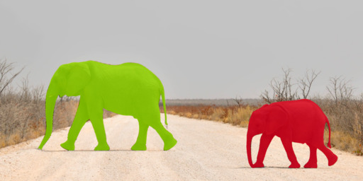
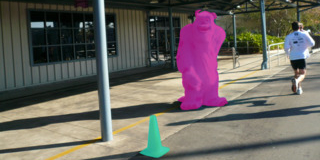
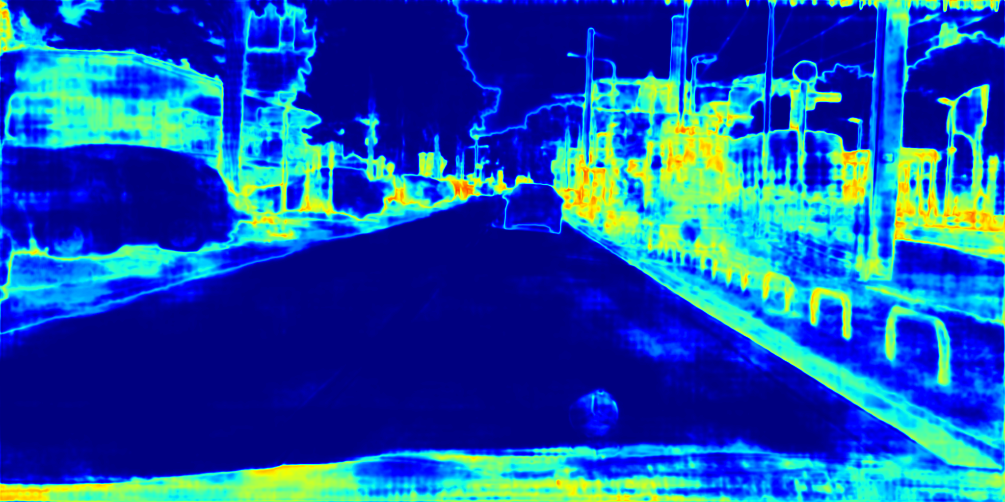
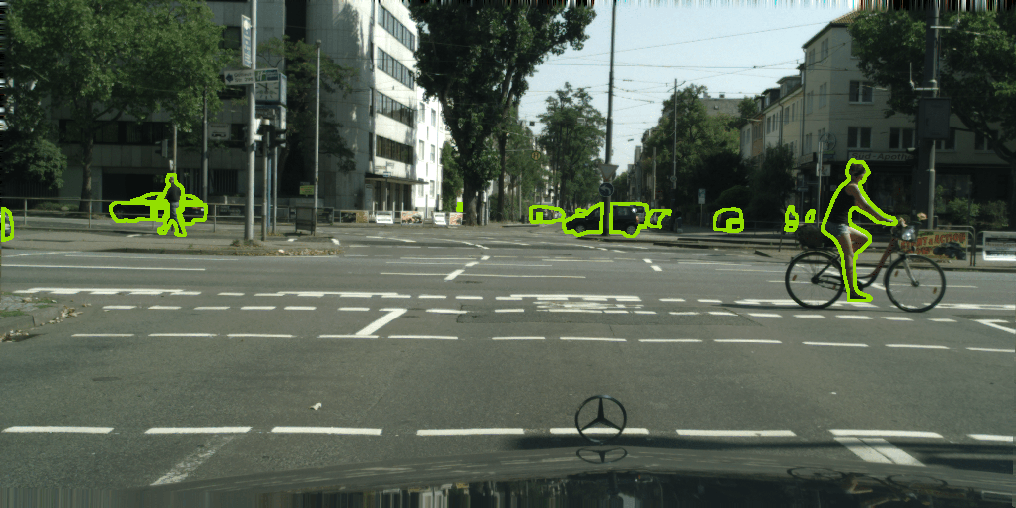
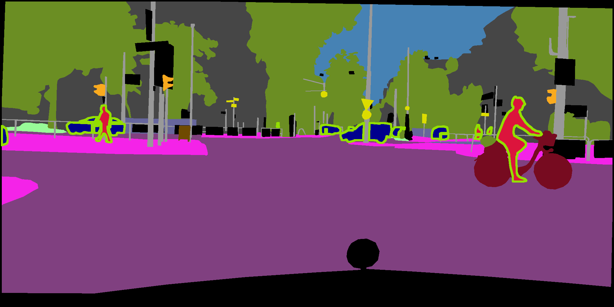
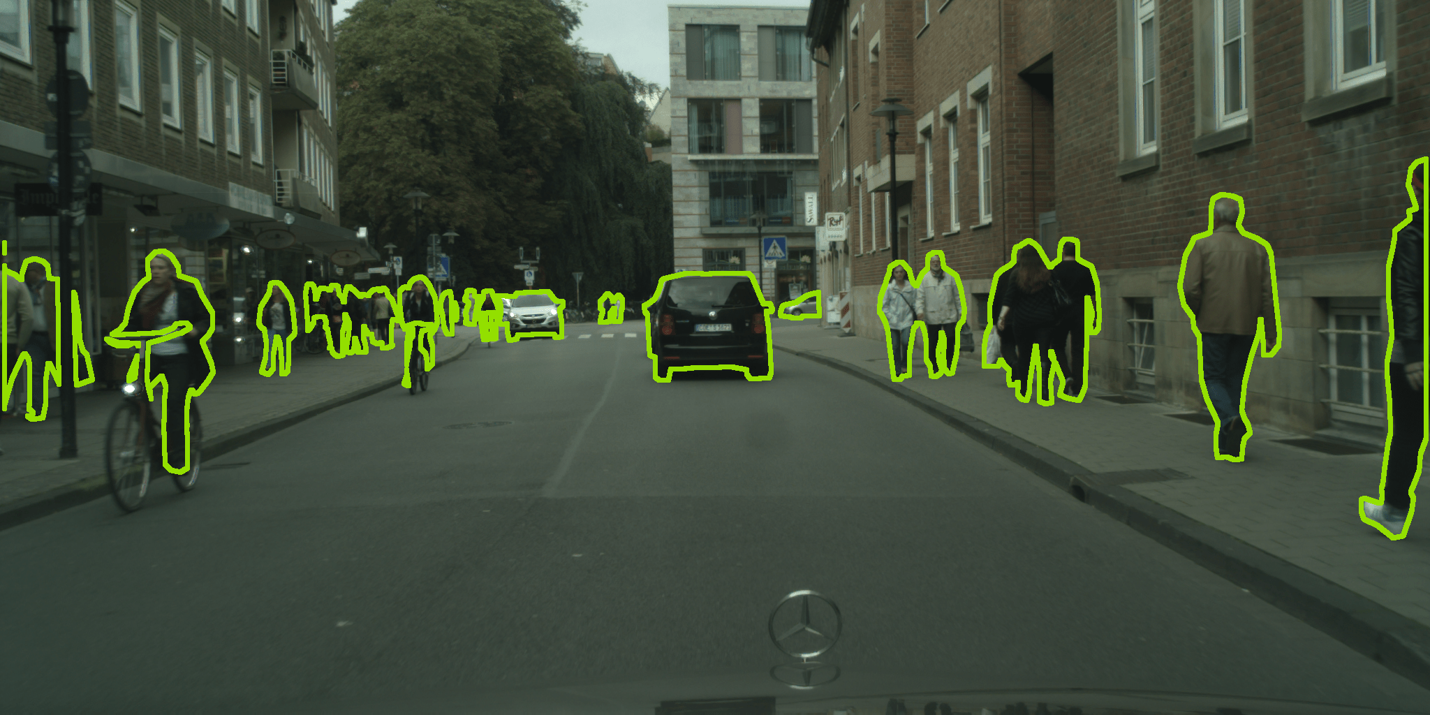
Let $H\times W$ denote the resolution of the images $x\in\mathcal{X}$. Then, the softmax output of a semantic segmentation DNN $f:\mathcal{X}\to(0,1)^{H\times W\times q}$ provides class-probabilities for image pixels, denoted as $z=(h,w)\in\mathcal{Z}$. Thus, the OoD detector must not only identify OoD images, but also give information about their pixel positions. To store these information, we generate OoD instance masks as illustrated in Fig. 4 by thresholding on the obtained OoD score and by distinguishing between connected components in the resulting OoD mask.

For semantic segmentation, the loss functions are computed for pixels of OoD objects instead of images. Let $\mathcal{Z}_{s}$ denote the set of pixel positions which belong to an OoD candidate $s\subseteq x$. The extension loss is computed equivalently to Eq. 2 as

$$\ell_{\mathrm{ext}}(s)=-\frac{1}{|\mathcal{Z}_{s}|}\sum_{z\in\mathcal{Z}_{s}}\frac{1}{q}\sum_{c=1}^{q}f^{k}_{z,c}(x)\;.$$ (9)

For two OoD candidates $s_{i}\subseteq x_{i},s_{j}\subseteq x_{j}$ with distance $d_{ij}$, the cluster loss is computed as

$$\ell_{\mathrm{cluster}}(s_{i},s_{j})=\frac{\alpha}{q+k}d_{ij}\sum_{c=1}^{q+k}\overline{f^{k}_{c}(x_{i})}~{}\overline{f^{k}_{c}(x_{j})}\;,$$ (10)

where

$$\overline{f^{k}_{c}(x)}=\frac{1}{|\mathcal{Z}_{s}|}\sum_{z\in\mathcal{Z}_{s}}f^{k}_{z,c}(x)$$ (11)

denotes the mean softmax probability over all pixels $z\in\mathcal{Z}_{s}$ for some class $c\in\{1,\ldots,q+k\}$.

For OoD detection in semantic segmentation, we adapt a meta regression approach [33, 34], using uncertainty measures such as the softmax entropy and further information which derives from the initial model’s output, to estimate the prediction quality on a segment-level. Here, a segment denotes a connected component in the semantic segmentation mask, which is predicted by the initial model. That is, meta regression is a post-processing approach to quantify uncertainty aggregated over segments, and considering that the model likely is highly uncertain if confronted with OoD objects, it can be applied for OoD detection. In contrast to image classification, where images are either OoD or not, semantic segmentation is performed on images which can contain in-distribution and OoD pixels at the same time. Aggregating uncertainty scores across segments simplifies the detection of OoD objects as contiguous OoD pixels, since it removes the high uncertainty for class boundaries.

For an initial DNN, we use the training data to fit a gradient boosting model as meta regressor, which then estimates segment-wise uncertainty scores $u(s)$ for all segments $s\subseteq x\in\mathcal{X}$.

5 Numerical Experiments

We perform several experiments for image classification on MNIST [21], FashionMNIST [42], CIFAR10 [20] and Animals10, as well as on Cityscapes [11] to evaluate our method for semantic segmentation. To this end, we extend the initial models by empty classes, i.e. , neurons in the final classification layer with randomly initialized weights, and fine-tune them on OoD data, retraining with fixed encoder. For evaluation, we provide accuracy scores - separately for known and novel classes - for image classification, (mean) Intersection over Union (IoU), precision and recall values for semantic segmentation.

The OoD classes in the following experiments were all chosen in a way that they are semantically far away from each other. For example, the Animals10 classes horse $(1)$, cow $(6)$ and sheep $(7)$ are semantically related, as they are all big animals which are mostly on the pasture, whereas elephant $(2)$ and spider $(8)$ are well separable classes, which is also visible in the two-dimensional feature space. However, we will also provide evaluation metrics averaged over multiple runs with randomly picked OoD classes in the appendix.

5.1 Experimental Setup

For each experiment, we consider the following dataset splits: the training data denotes images with ground truth for the initially known classes. We train the initial model on these images and replay them during the training of the extended model to avoid catastrophic forgetting. The test data consist of unlabeled images which include both, known and unknown classes. This dataset is fed into the OoD detector to identify OoD data, on which the model gets extended. The evaluation dataset includes images with ground truth for known and novel classes and is used to evaluate the models. If there are such labels available for the test data, evaluation images may be the same as the test images.

Our approach requires prior OoD detection. Here, we only provide the experimental setup for fine-tuning the extended model. For all experiments, we tuned the weighting parameters $\lambda_{1},\lambda_{2},\lambda_{3}$ in Sec. 3 by observing all loss functions separately over several epochs using different parameter configurations to ensure that each loss term decreases. The following descriptions of the experiments, sorted by the datasets, include the network architecture, the known and novel classes, information about the dataset splits and the generation of the distance matrix. For further information about the experiments, which also includes the TwoMoons experiment, we refer to the appendix.

MNIST

We employ a shallow neural network consisting of two convolutional layers, each followed by a ReLU activation function and max pooling, and a fully connected layer. From the digits $0,\ldots,9$, we select $0,5$ and $7$ as novel classes. All images in the MNIST training set which belong to these classes are excluded from our training data. The MNIST test images compose our test set, and together with the original labels, our evaluation set. The distance matrix is computed as pixel-wise Euclidean distance between the OoD images.

Figure 5: Visualized ground truth (left) and prediction of the MNIST dataset by the initial (middle) and extended (right) model. The three novel classes $0,5$ and $7$ are outlined in orange. The extended model’s accuracy is $\sim 94\%$.

Figure 6: Visualized ground truth (left) and prediction of the FashionMNIST dataset by the initial (middle) and extended (right) model. The two novel classes $1$ and $8$ are outlined in orange. The extended model’s accuracy is $\sim 85\%$.

FashionMNIST

Using the same network architecture as for MNIST, our initial model is trained on eight out of ten classes, excluding the classes trouser (1) and bag (8). Our dataset splits are created analogously to those from MNIST. Also the distance matrix is obtained analogously by computing the pixel-wise Euclidean distances between the OoD images.

CIFAR10

The setting for CIFAR10 differs slightly from the other experiments to ensure comparability with existing approaches. Thus, as initial model, we employ a ResNet18 which is trained on the whole CIFAR10 training split, including all ten classes. For testing, we enrich the CIFAR10 test split with images from CIFAR100. Therefore, we split CIFAR100 into an unlabeled and a labeled subset: the classes $\{0,\ldots,49\}$ are possible OoD candidates, thus, all samples belonging to these classes are considered to be unlabeled. We extend the CIFAR10 test data by the classes apple (0) and clock (22), mapping them onto the labels (10) and (11), respectively. As before, we evaluate our models on the labeled test data. The labeled CIFAR100 subset includes the classes $\{50,\ldots,99\}$ and is used together with the CIFAR10 training data to train a ResNet18 as an embedding network. To compute the distances, we feed the whole test data into this embedding network and extract the features of the penultimate layer. These are further projected into a 2D space with UMAP. Then, the distance matrix is computed as the pixel-wise Euclidean distance between the 2D representations of the OoD images.

Figure 7: Visualized ground truth (left) and prediction of the Animals10 dataset by the initial (middle) and extended (right) model. The four novel classes $3,4,8$ and $9$ are outlined in orange. The extended model’s accuracy is $\sim 95\%$.

Figure 8: Visualized ground truth (left) and prediction of the CIFAR10 dataset by the initial (middle) and extended (right) model. The two novel classes $10$ and $11$ are outlined in orange. The extended model’s accuracy is $\sim 89\%$.

Image Classification
			supervised		unsupervised		ablation studies
dataset	OoD	accuracy	initial	oracle	ours	baseline	$-$detection	$--$distance
MNIST	$0~{}~{}5~{}~{}7$	known	$96.68\%$	$98.54\%$	$\mathbf{96.20\%}$	$95.94\%$	$97.45\%$	$96.54\%$
		novel	-	$95.85\%$	$\mathbf{97.94\%}$	$84.62\%$	$74.52\%$	$97.00\%$
FashionMNIST	$1~{}~{}8$	known	$81.54\%$	$83.75\%$	$81.41\%$	$\mathbf{85.08\%}$	$81.89\%$	$81.39\%$
		novel	-	$90.83\%$	$90.05\%$	$\mathbf{92.85\%}$	$89.90\%$	$95.00\%$
CIFAR10	$10~{}~{}11$	known	$91.45\%$	$91.86\%$	$\mathbf{90.51\%}$	$90.29\%$	$88.90\%$	$86.94\%$
		novel	-	$89.53\%$	$\mathbf{70.00\%}$	$33.40\%$	$78.80\%$	$87.00\%$
Animals10	$3~{}~{}4~{}~{}8~{}~{}9$	known	$96.29\%$	$95.80\%$	$\mathbf{93.76\%}$	$92.78\%$	$94.46\%$	$95.20\%$
		novel	-	$97.65\%$	$\mathbf{96.68\%}$	$72.59\%$	$97.02\%$	$97.90\%$

Table 1: Quantitative evaluation of the image classification experiments. For all evaluated models, the accuracy is stated separately for the previously-known and the unlabeled novel classes. The highest scores for the unsupervised approaches are bolded.

Animals10

As initial model, we employ a ResNet18 which is trained on six out of ten classes. As novel classes we selected butterfly (3), chicken (4), spider (8) and squirrel (9). The dataset splits are obtained analogously to those from MNIST. The distances are computed as for CIFAR10, but employing a DenseNet201, which is trained on ImageNet with $1,\!000$ classes, as embedding network.

Cityscapes

For comparison reasons with the baseline, we adapt the experimental setup from [39], where the class labels human (person, rider), car and bus are excluded from the $19$ Cityscapes evaluation classes. Like the baseline, we extend the DNN by two empty classes and exclude the class bus from the evaluation. Thus, we train a semantic segmentation DeepLabV3+ with WideResNet38 backbone on $2,\!500$ training samples with $15$ trainable classes. We apply meta regression to the Cityscapes test data and crop out image patches tailored to the predicted OoD segments, i.e. , connected component of OoD pixels. Afterwards, we compute distances between these image patches analogously to Animals10 as the Euclidean distances between 2D representations of features which we obtain by feeding the patches into a DenseNet201 trained on $1,\!000$ ImageNet classes.

5.2 Evaluation & Ablation Studies

We compare our evaluation results to the following baselines. For image classification, we employ the k-means clustering algorithm to pseudo-label the OoD data samples and fine-tune the model on the pseudo-labeled data using the cross-entropy loss. For semantic segmentation, we compare with the method presented in [39], which also employs clustering algorithms in the embedding space to obtain pseudo-labels. Furthermore, to get an idea of the maximum achievable performance, we train oracle models which have learned all available classes in a fully supervised manner.

For the ablation studies, we evaluate our image classification approach on “clean” OoD data ($-$detection). Therefore, we do not detect the OoD samples in the test data by thresholding on some anomaly score, but by considering the ground truth. In this way, we simulate a perfect OoD detector. Since the results of our method are also affected by the quality of the distance matrix, we further analyze our method for a synthetic distance matrix ($--$distance), where two OoD samples $x_{i},x_{j}\in\mathcal{X}^{\mathrm{OoD}}$ have a distance $d(x_{i},x_{j})=0$ if they stem from the same class, $d(x_{i},x_{j})=1$ otherwise. Thus, the OoD samples are labeled by the distance matrix and the fine-tuning is supervised, allowing a pure comparison of our loss functions with the cross-entropy loss. We do not provide ablation studies for semantic segmentation, since the Cityscapes test data does not include publicly available annotations.

Image Classification

As shown in Tab. 1 and visualized in Figs. 6, 6, 8 and 8, our approach exceeds the baseline’s accuracy for novel classes by $36.60$ and $24.09$ percentage points (pp) for CIFAR10 and Animals10, respectively. This is mainly caused by in-distribution samples which are false positive OoD predictions, or by OoD samples which are embedded far away from their class centroids. Consequently, different OoD classes are assigned to the same cluster by the k-means algorithm. As our approach uses soft labels, the DNN is more likely to reconsider the choice of the OoD detector during fine-tuning.

In the ablation studies, we omit the OoD detector ($-$detection) and select the OoD samples based on their ground truth instead. Thereby, we observe an improvement of the accuracy of novel classes for the CIFAR10 and Animals10 datasets, while the performance remains constant for FashionMNIST and significantly decreases for MNIST. We further compute a ground truth distance matrix ($--$distance) with distances $0$ and $1$ for samples belonging to the same or to different classes, respectively. Since this is supervised fine-tuning, these DNNs are comparable to oracles. We observe, that the oracles tend to perform better on the initial and worse on the novel classes. However, this might be a consequence of the class-incremental learning.

(a)

(b)

(c)

(d)

(e) image

(f) ground truth

(g) ours

(h) baseline

Figure 9: Visual comparison of the segmentation masks produced by our method and by the baseline for two image cutouts from the Cityscapes validation dataset. The ground truth contours of the novel classes are highlighted with green.

Semantic Segmentation
			supervised		unsupervised
dataset	class	metric	initial	oracle	ours	baseline
Cityscapes	$0,\ldots,14$	mean IoU	$56.99\%$	$77.28\%$	$\mathbf{59.72\%}$	$57.52\%$
	$15$ (human)	IoU	-	$81.90\%$	$33.87\%$	$\mathbf{40.22\%}$
	$16$ (car)	IoU	-	$94.94\%$	$\mathbf{84.14\%}$	$81.27\%$
	$0,\ldots,14$	mean precision	$65.75\%$	$88.03\%$	$\mathbf{84.63\%}$	$78.53\%$
	$15$ (human)	precision	-	$89.22\%$	$37.80\%$	$\mathbf{68.74\%}$
	$16$ (car)	precision	-	$96.83\%$	$\mathbf{87.11\%}$	$86.56\%$
	$0,\ldots,14$	mean recall	$80.88\%$	$85.38\%$	$65.38\%$	$\mathbf{65.78\%}$
	$15$ (human)	recall	-	$90.90\%$	$\mathbf{76.54\%}$	$49.65\%$
	$16$ (car)	recall	-	$97.99\%$	$\mathbf{96.11\%}$	$93.05\%$

Table 2: Quantitative evaluation of the semantic segmentation experiment on the Cityscapes dataset. IoU, precision and recall values are provided for both novel classes as well as averaged over the previously-known classes. The highest scores for the unsupervised approaches are bolded.

Semantic Segmentation

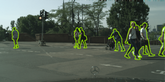
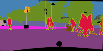
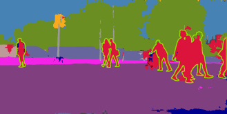
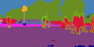
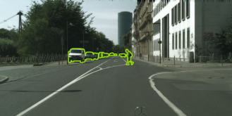
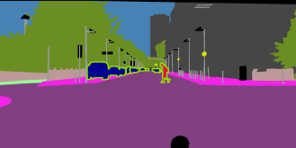
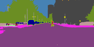
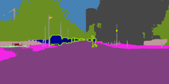
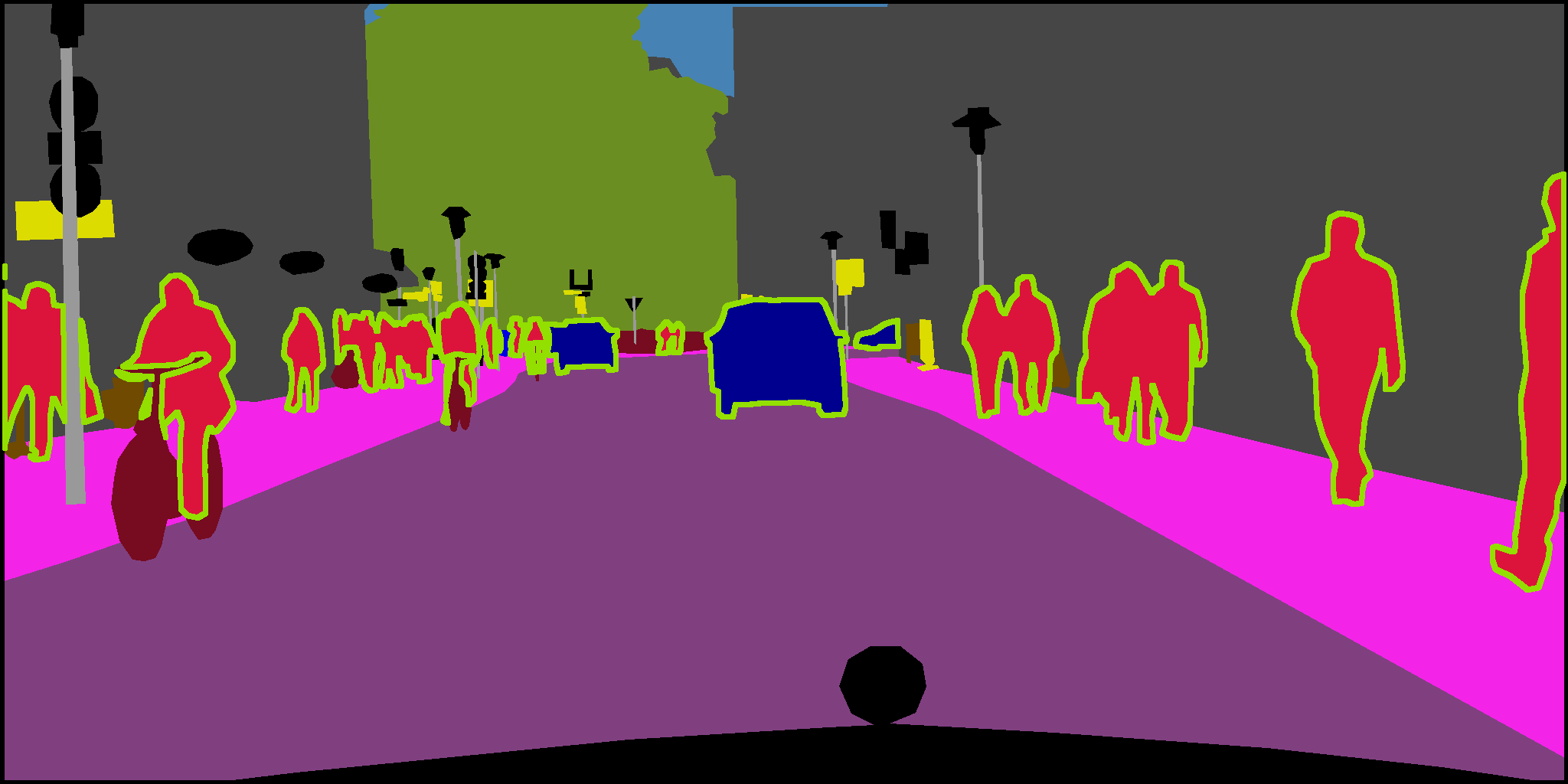
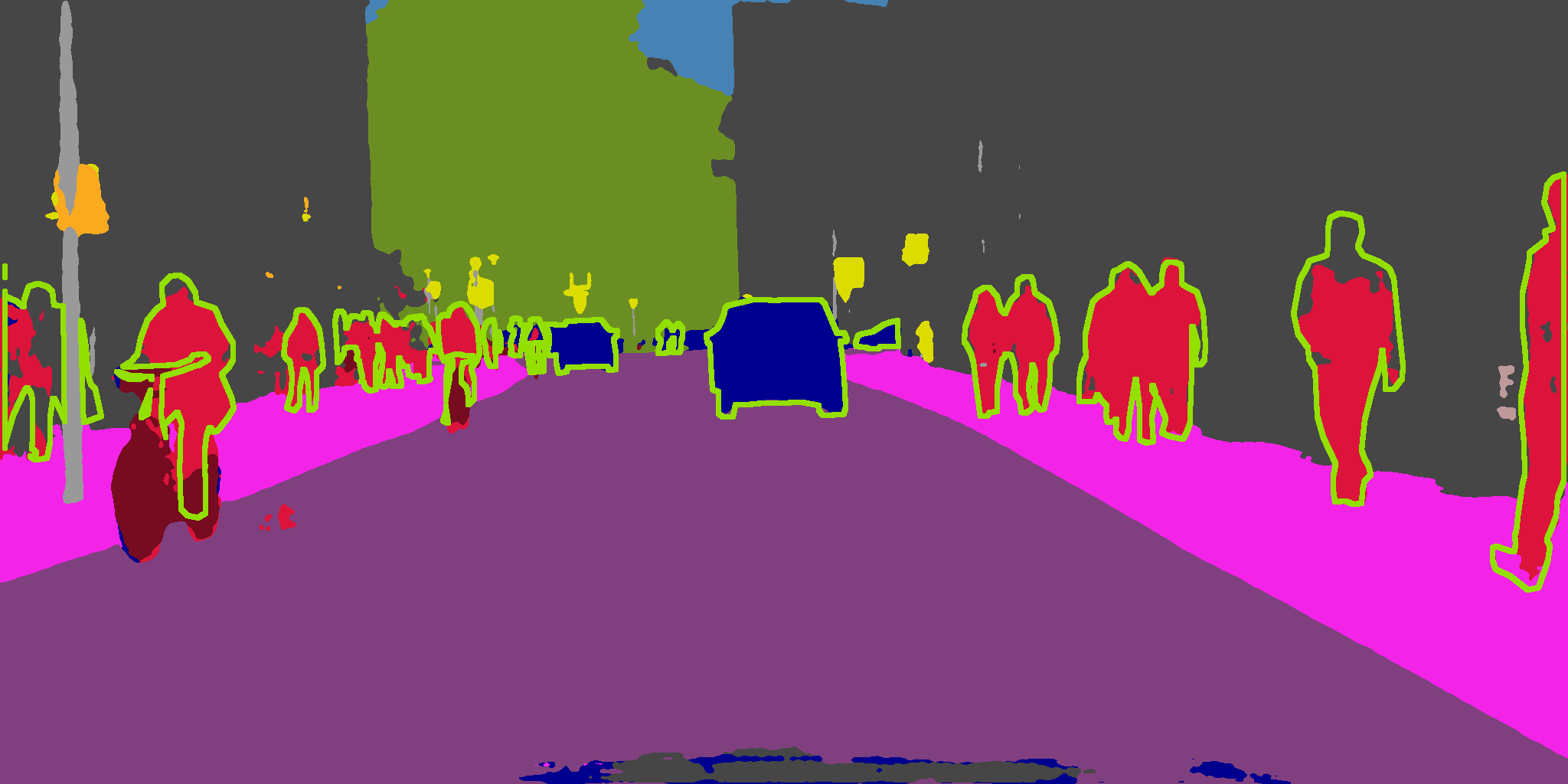
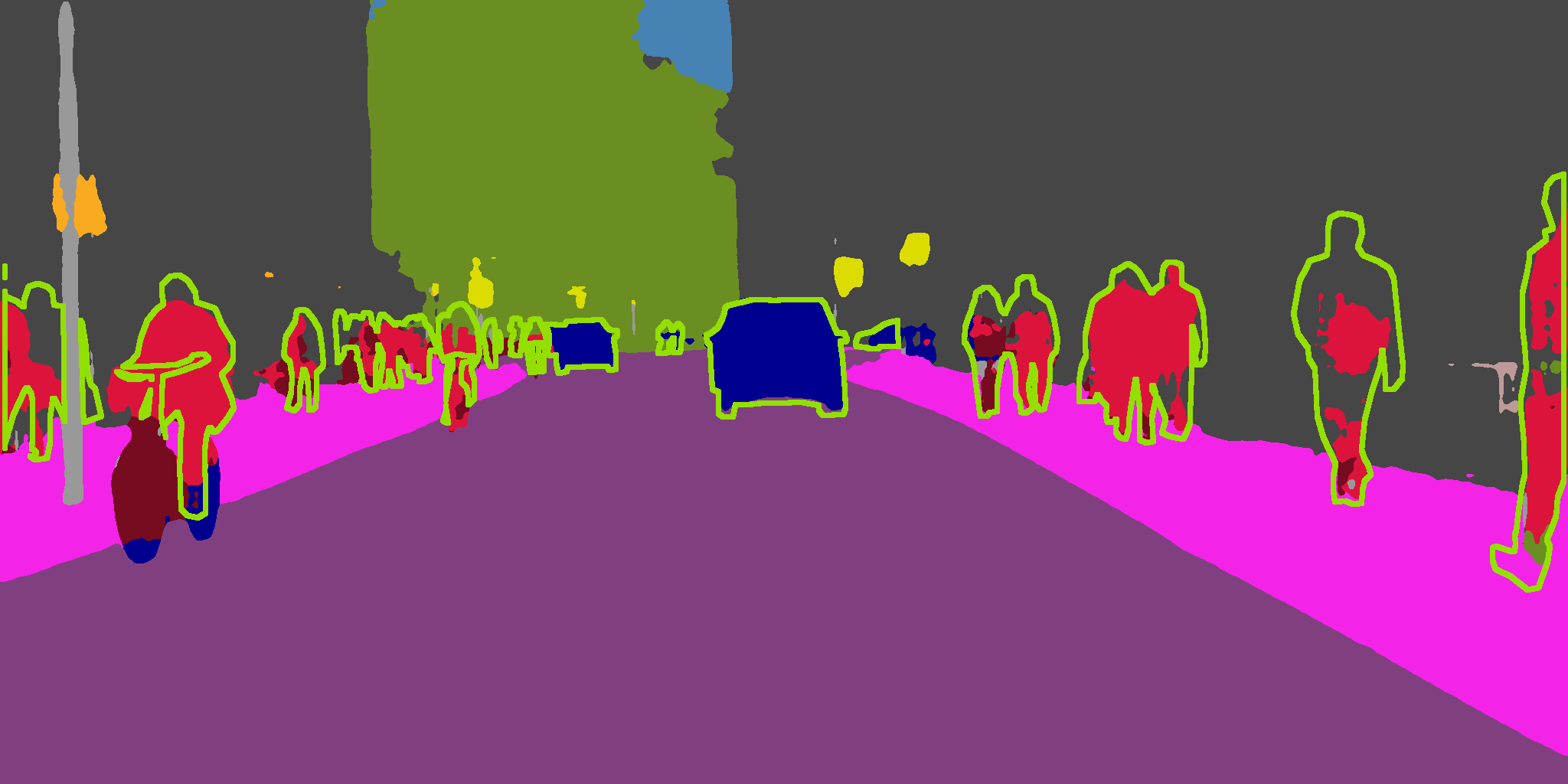
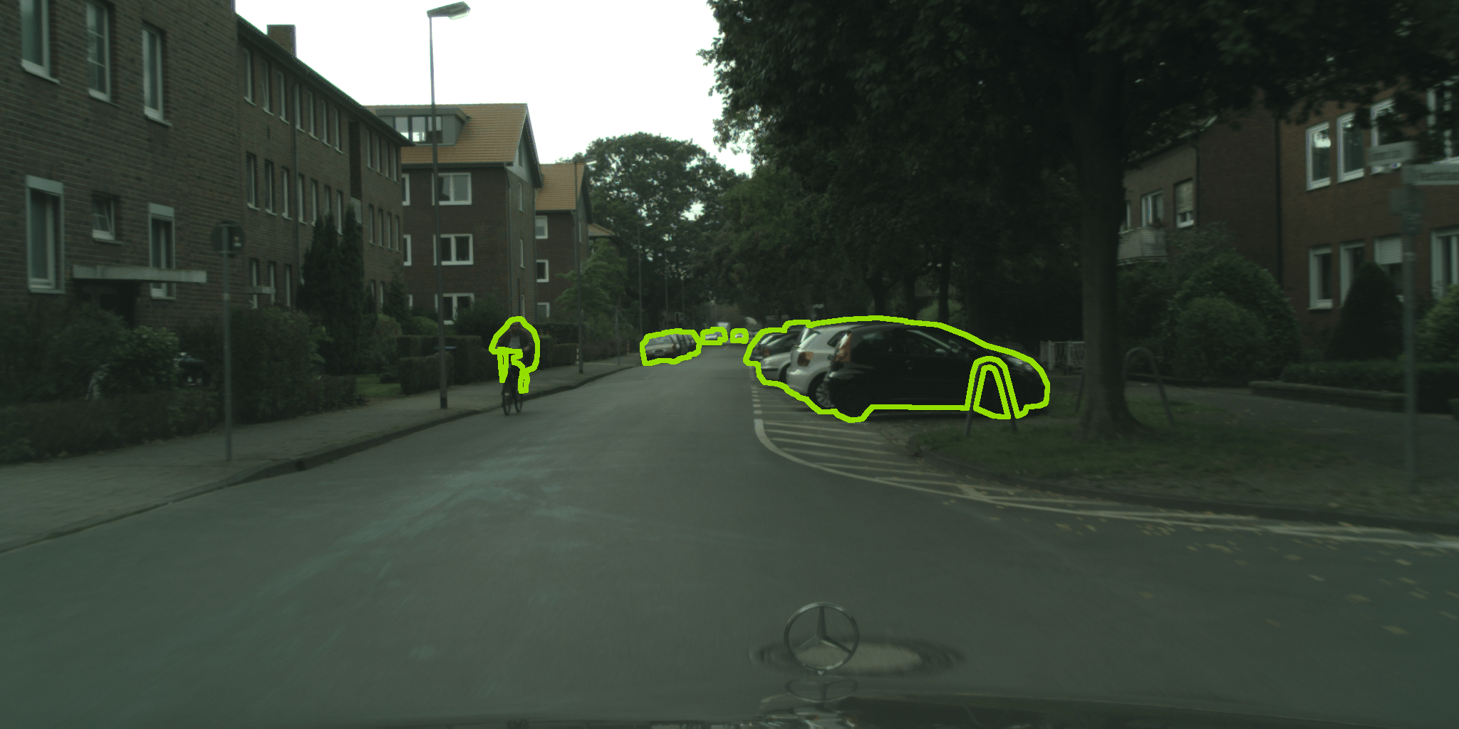
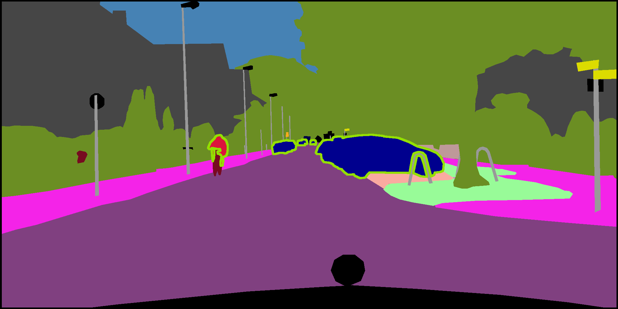
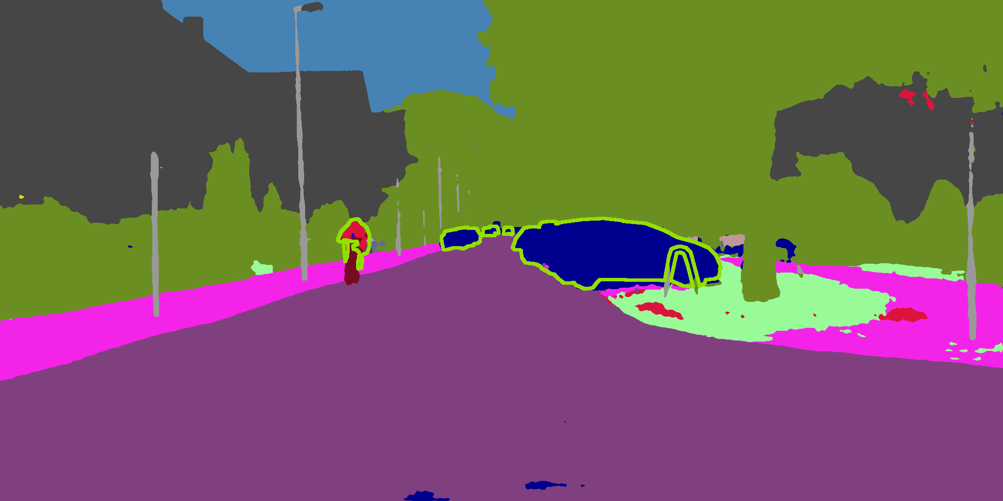
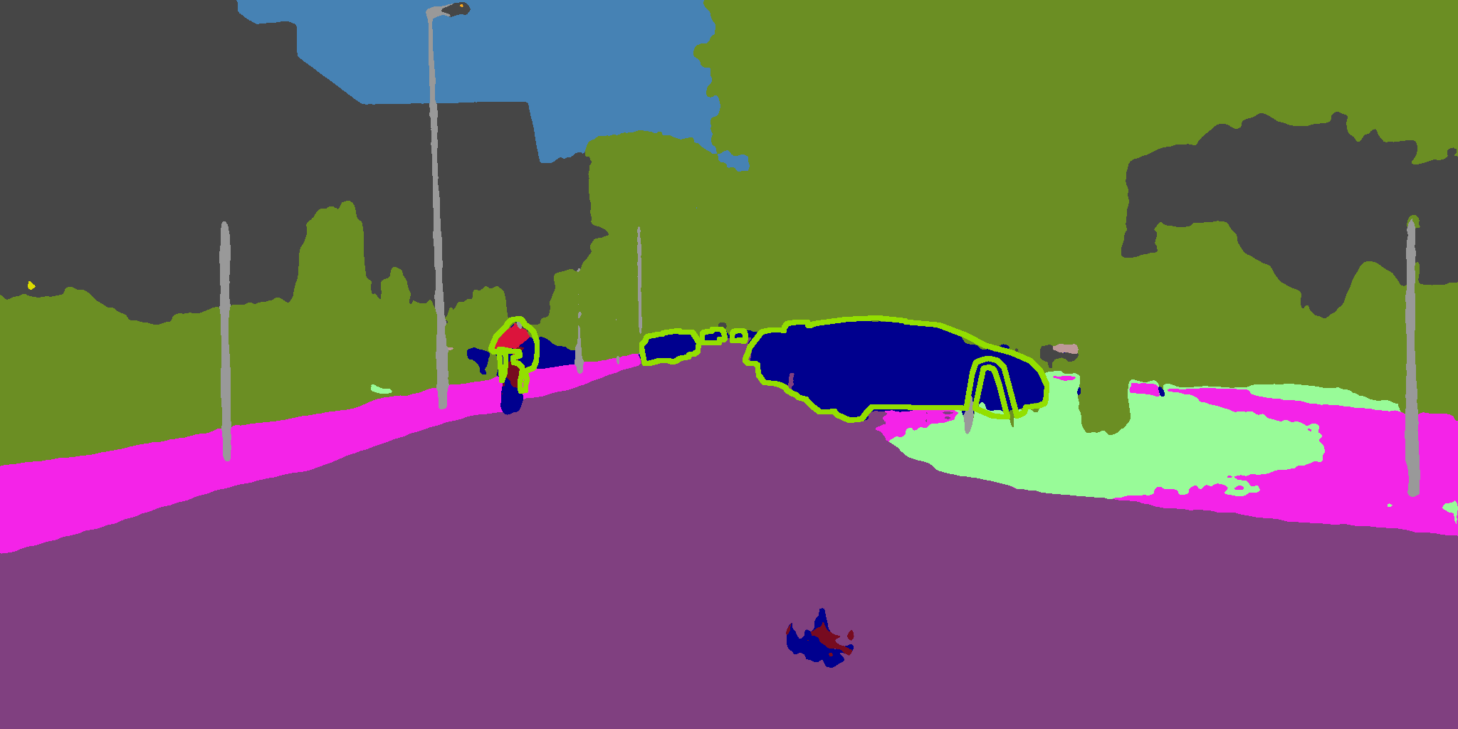
The quantitative results of our semantic segmentation method, reported in Tab. 2, demonstrate, that the empty classes are “filled” with the novel concepts human and car. Thereby, the performance on the previously-known classes is similar to the baseline even without including a distillation loss [28]. For the car class, our method outperforms the baseline with respect to IoU ($+2.87$ pp), precision ($+0.55$ pp) and recall ($+3.06$ pp). We lose performance in terms of IoU for the human class due to a higher tendency for false positives. However, the false negative rate is significantly reduced, which is indicated by an increase in the recall value of $26.89$ pp. The improved recall score is also visible in Fig. 9, showing two examples from the Cityscapes validation dataset. In the top row, several pedestrians are crossing the street, which are mostly segmented by our DNN, whereas the baseline DNN mostly misses the persons in the center as well as all heads. In the bottom row, the person in front of the car is completely overlooked by the baseline, and also some cars in the background are missed.

When examining the OoD masks, we observed that the connected components are often very extensive, which is caused by neighboring OoD objects. Thus, the embedding space contains many large image patches which are not tailored to a single OoD object, but rather to a number of parked cars, a crowd of people or even a bicyclist riding next to a car, which appreciably impairs our results.

6 Conclusion & Outlook

In our work, we proposed a solution to open world classification for image classification and semantic segmentation by learning novel classes in an unsupervised manner. We suggested to postulate empty classes, which allow one to capture newly observed classes in an incremental learning approach. This way, we allow our model to detect new classes in a flexible manner, potentially whitewashing mistakes of previous OoD detectors.

As our method employs several hyperparameters, e.g. , to specify the number of novel empty classes, we envision an automatic derivation of the optimal number of new classes as future work. In this regard, replacing the Elbow method in the eventual clustering by more suitable criteria appears desirable [36]. Moreover, we shall investigate approaches to improve the generalizability of our approach to embedding models of arbitrary kind to derive distance matrices, not being tailored to specific datasets. Furthermore, the semantic segmentation performance could be improved by incorporating depth information into the OoD segmentation method to obtain OoD candidates on instance- instead of segment-level.

Appendix

Appendix A More Details on Experiments

A.1 TwoMoons

As a proof of concept, consider a simple binary classification problem in the plane. As in-distribution data $1000$ samples are drawn from the Two Moons dataset with noise $=0.1$. Additionally, $100$ OoD data samples are drawn from a uniform distribution over $[-4,4]^{2}$, as illustrated in Fig. 2. Then, a shallow neural network, consisting of $4$ fully connected layers, is trained on these samples to minimize the cross entropy with respect to the Two Moons data while maximizing the entropy on the OoD data. As test data, another $750$ samples are drawn from the Two Moons dataset, together with $500$ OoD samples belonging to three blobs, centered at $c_{1}=(-1.5,-0.95),c_{2}=(2.5,1.5)$ and $c_{3}=(3,-1)$, respectively, with $0.25$ standard deviation. These blobs represent the novel classes. The test data is then fed into the trained model, and is considered to be OoD if the softmax entropy exceeds a threshold of $0.8$. Finally, the initial model is extended by three empty classes in the last layer and then fine-tuned on the Two Moons training samples plus the OoD samples detected in the test data. The OoD data is clustered into the empty classes through our proposed loss function, without requiring any previous (pseudo-)labeling.

A.2 Training Parameters

We provide an overview of the training parameters for each experiment in Tab. 3. We performed experiments using the Adam and the SGD optimizer as well as different batch sizes. Only the batch size for semantic segmentation was bounded by memory limitations. The hyperparameters which are related to the loss functions, namely $\alpha,\lambda_{1},\lambda_{2},\lambda_{3}$, were selected by trying out and monitoring the course of the loss functions.

Appendix B Evaluation Metrics for Randomized OoD Classes

Our approach assumes, that novel classes are well separable in the feature space. Thus, we have selected suitable classes by hand. In Tab. 4, we provide evaluation metrics which are averaged over 5 runs with randomly selected classes, respectively. In particular, for FashionMNIST, we observe a large standard deviation of $27.61\%$ in the accuracy of novel classes. Our method fails, whenever the novel classes are t-shirt/top $(0)$ or shirt $(6)$, which are semantically similar and also not separable in the feature space. The same holds for Animals10 regarding the classes horse, $(1)$, cow $(6)$ and sheep $(7)$.

Appendix C OoD Detection

(a) MNIST: $0,5,7$

(b) FashionMNIST: $1,8$

(c) Cifar10: $11,12$

(d) Animals10: $3,4,8,9$

Figure 10: Visualization of the softmax entropy, that the initial models exhibit on samples of known and OoD classes, respectively.

(a) MNIST: $0,5,7$

(b) FashionMNIST: $1,8$

(c) Cifar10: $11,12$

(d) Animals10: $3,4,8,9$

Figure 11: Visualization of the softmax entropy per data sample, that the initial models exhibits on test samples.

(a)

(b)

(c)

(d)

(e) image

(f) ground truth

(g) ours

(h) baseline

Figure 12: Visual comparison of the segmentation masks produced by our method and by the baseline for two images from the Cityscapes validation dataset. The ground truth contours of the novel classes are highlighted with green.

dataset	$\#$ empty classes	$\#$ epochs	optimizer	learning rate	momentum	weight decay	batch size	$\alpha$	$\lambda_{1}$	$\lambda_{2}$	$\lambda_{3}$
MNIST	3	30	adam	1e-2	-	-	2500	5	0.45	0.45	0.1
FashionMNIST	2	30	sgd	1e-2	0	0	500	2.5	0.45	0.45	0.1
Cifar10	2	30	sgd	1e-2	0.9	1e-4	1000	5	0.45	0.45	0.1
Animals10	4	30	adam	5e-3	-	-	1000	2.5	0.45	0.45	0.1
Cityscapes	2	200	adam	5e-3	-	-	10	2.5	0.375	0.375	0.25

Table 3: Overview of training parameters for each dataset.

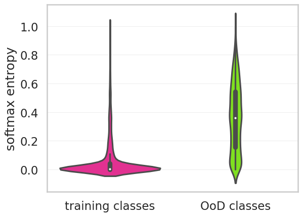
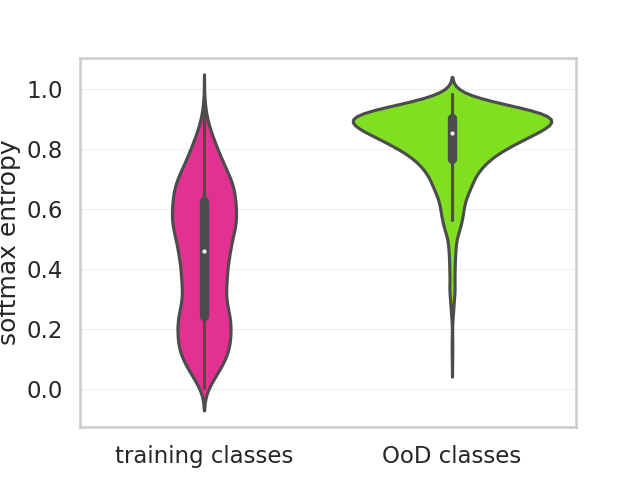
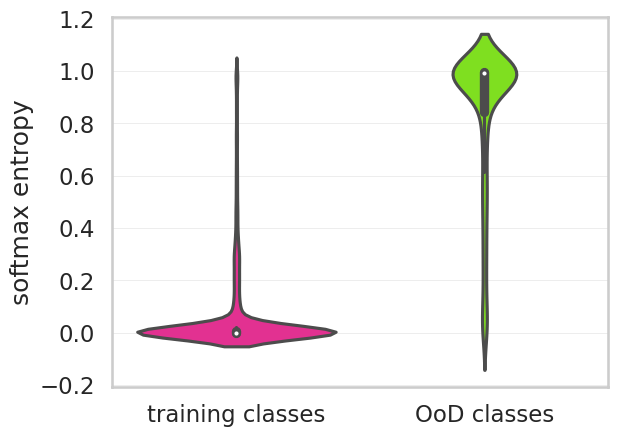
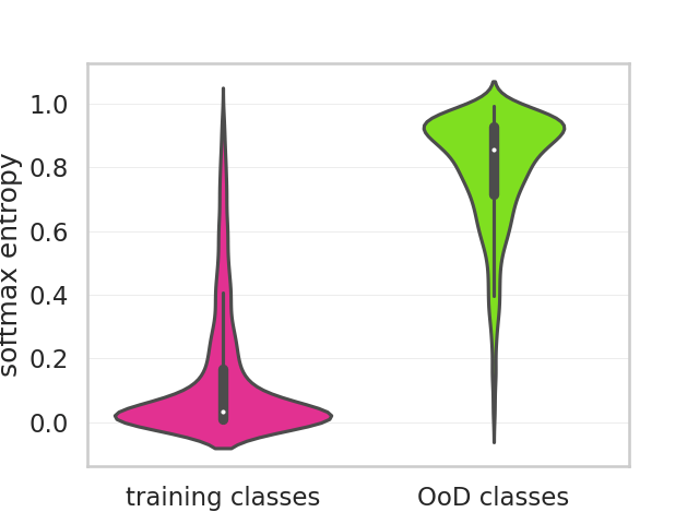
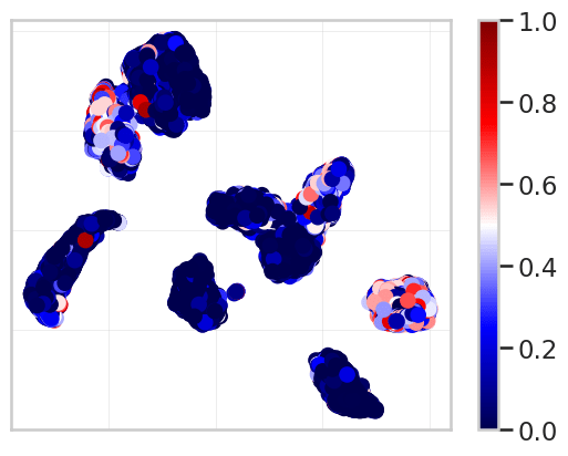
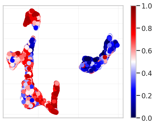
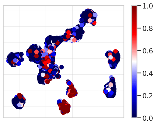
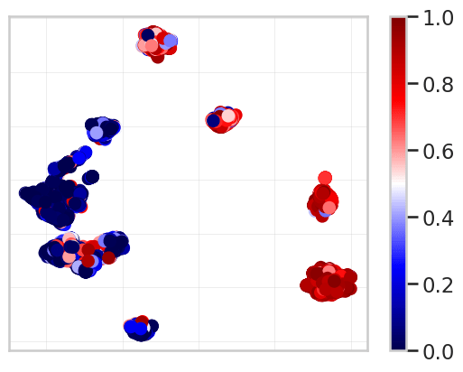
For image classification, we employed entropy maximization during training the initial model. The softmax entropy for the test data is visualized as a summary statistic in Fig. 10 and sample-wise in Fig. 11. We observe that the DNN exhibits high entropy scores on OoD data for all datasets except MNIST. However, the entropy for MNIST in-distribution data is sufficiently small, so that we detect most OoD samples using a threshold of $\tau=0.1$. Further, the initial FashionMNIST DNN is uncertain regarding the in-distribution classes t-shirt/top $(0)$, pullover $(2)$ and shirt $(6)$. However, this may be aleatoric uncertainty. To avoid too many false positive OoD predictions, we choose a high threshold $\tau=0.75$. For the remaining datasets, in-distribution and OoD samples are well separable by the softmax entropy, thus, there is a large interval of proper thresholds.

Image Classification
dataset	$\#$OoD	accuracy	initial	ours
FashionMNIST	2	known	$84.72\pm 03.25\%$	$82.78\pm 02.18\%$
		novel	-	$63.42\pm 27.61\%$
Animals10	4	known	$97.02\pm 00.63\%$	$94.70\pm 00.59\%$
		novel	-	$66.79\pm 25.82\%$

Table 4: Quantitative evaluation of the FashionMNIST and Animals10 experiments, averaged over $5$ runs with randomly selected OoD classes, each. For all evaluated models, the accuracy is stated separately for the previously-known and the unlabeled novel classes.

Appendix D Semantic Segmentation

We provide some more qualitative semantic segmentation results in Fig. 12, for which our method outperforms the baseline. Furthermore, we also give an example in Fig. 13, where regions which come along with a high softmax entropy are wrongly predicted as the novel class human.

(a) predicted segmentation

(b) softmax entropy

Figure 13: For highly uncertain regions, the extended DNN tends to predict the novel human class, which causes the low precision score.

References

- [1] Abhijit Bendale and Terrance E. Boult. Towards open world recognition. 2015 IEEE Conference on Computer Vision and Pattern Recognition (CVPR), pages 1893–1902, 2015.
- [2] Max Bucher, Tuan-Hung Vu, Matthieu Cord, and Patrick Pérez. Zero-shot semantic segmentation. ArXiv, abs/1906.00817, 2019.
- [3] Mathilde Caron, Hugo Touvron, Ishan Misra, Hervé Jégou, Julien Mairal, Piotr Bojanowski, and Armand Joulin. Emerging properties in self-supervised vision transformers. In 2021 IEEE/CVF International Conference on Computer Vision, ICCV 2021, Montreal, QC, Canada, October 10-17, 2021, pages 9630–9640. IEEE, 2021.
- [4] Gert Cauwenberghs and Tomaso A. Poggio. Incremental and decremental support vector machine learning. In NIPS, 2000.
- [5] Jun Cen, Peng Yun, Junhao Cai, Michael Yu Wang, and Ming Liu. Deep metric learning for open world semantic segmentation. In Proceedings of the IEEE/CVF International Conference on Computer Vision (ICCV), pages 15333–15342, October 2021.
- [6] Jun Cen, Peng Yun, Junhao Cai, Michael Yu Wang, and Ming Liu. Deep metric learning for open world semantic segmentation. 2021 IEEE/CVF International Conference on Computer Vision (ICCV), pages 15313–15322, 2021.
- [7] Jun Cen, Peng Yun, Shiwei Zhang, Junhao Cai, Di Luan, Michael Yu Wang, Meilin Liu, and Mingqian Tang. Open-world semantic segmentation for lidar point clouds. ArXiv, abs/2207.01452, 2022.
- [8] Robin Chan, Krzysztof Lis, Svenja Uhlemeyer, Hermann Blum, Sina Honari, Roland Siegwart, Pascal Fua, Mathieu Salzmann, and Matthias Rottmann. Segmentmeifyoucan: A benchmark for anomaly segmentation. In Thirty-fifth Conference on Neural Information Processing Systems Datasets and Benchmarks Track (Round 2), 2021.
- [9] Robin Chan, Matthias Rottmann, and Hanno Gottschalk. Entropy maximization and meta classification for out-of-distribution detection in semantic segmentation. In Proceedings of the IEEE/CVF International Conference on Computer Vision (ICCV), pages 5128–5137, October 2021.
- [10] Ting Chen, Simon Kornblith, Kevin Swersky, Mohammad Norouzi, and Geoffrey E. Hinton. Big self-supervised models are strong semi-supervised learners. In Advances in Neural Information Processing Systems 33: Annual Conference on Neural Information Processing Systems 2020, NeurIPS 2020, December 6-12, 2020, virtual, 2020.
- [11] Marius Cordts, Mohamed Omran, Sebastian Ramos, Timo Rehfeld, Markus Enzweiler, Rodrigo Benenson, Uwe Franke, Stefan Roth, and Bernt Schiele. The cityscapes dataset for semantic urban scene understanding. 2016 IEEE Conference on Computer Vision and Pattern Recognition (CVPR), pages 3213–3223, 2016.
- [12] Jia Deng, Wei Dong, Richard Socher, Li-Jia Li, Kai Li, and Li Fei-Fei. Imagenet: A large-scale hierarchical image database. In 2009 IEEE Conference on Computer Vision and Pattern Recognition, pages 248–255, 2009.
- [13] Martin Ester, Hans-Peter Kriegel, Jörg Sander, and Xiaowei Xu. A density-based algorithm for discovering clusters in large spatial databases with noise. In KDD, 1996.
- [14] Wouter Van Gansbeke, Simon Vandenhende, Stamatios Georgoulis, and Luc Van Gool. Unsupervised semantic segmentation by contrasting object mask proposals. 2021 IEEE/CVF International Conference on Computer Vision (ICCV), pages 10032–10042, 2021.
- [15] Spyros Gidaris, Praveer Singh, and Nikos Komodakis. Unsupervised representation learning by predicting image rotations. In 6th International Conference on Learning Representations, ICLR 2018, Vancouver, BC, Canada, April 30 - May 3, 2018, Conference Track Proceedings. OpenReview.net, 2018.
- [16] Jean-Bastien Grill, Florian Strub, Florent Altché, Corentin Tallec, Pierre H. Richemond, Elena Buchatskaya, Carl Doersch, Bernardo Ávila Pires, Zhaohan Guo, Mohammad Gheshlaghi Azar, Bilal Piot, Koray Kavukcuoglu, Rémi Munos, and Michal Valko. Bootstrap your own latent - A new approach to self-supervised learning. In Advances in Neural Information Processing Systems 33: Annual Conference on Neural Information Processing Systems 2020, NeurIPS 2020, December 6-12, 2020, virtual, 2020.
- [17] Jiangpeng He and Feng Zhu. Unsupervised continual learning via pseudo labels. ArXiv, abs/2104.07164, 2021.
- [18] Dan Hendrycks, Mantas Mazeika, and Thomas G. Dietterich. Deep anomaly detection with outlier exposure. ArXiv, abs/1812.04606, 2018.
- [19] Nicolas Jourdan, Eike Rehder, and Uwe Franke. Identification of uncertainty in artificial neural networks. 2019.
- [20] Alex Krizhevsky. Learning multiple layers of features from tiny images. 2009.
- [21] Yann LeCun, Léon Bottou, Yoshua Bengio, and Patrick Haffner. Gradient-based learning applied to document recognition. Proc. IEEE, 86:2278–2324, 1998.
- [22] Chunyuan Li, Jianwei Yang, Pengchuan Zhang, Mei Gao, Bin Xiao, Xiyang Dai, Lu Yuan, and Jianfeng Gao. Efficient self-supervised vision transformers for representation learning. In The Tenth International Conference on Learning Representations, ICLR 2022, Virtual Event, April 25-29, 2022. OpenReview.net, 2022.
- [23] Tsung-Yi Lin, Michael Maire, Serge J. Belongie, James Hays, Pietro Perona, Deva Ramanan, Piotr Dollár, and C. Lawrence Zitnick. Microsoft coco: Common objects in context. In European Conference on Computer Vision, 2014.
- [24] Quan Liu, Youpeng Wen, Jianhua Han, Chunjing Xu, Hang Xu, and Xiaodan Liang. Open-world semantic segmentation via contrasting and clustering vision-language embedding. In European Conference on Computer Vision, 2022.
- [25] J. MacQueen. Some methods for classification and analysis of multivariate observations. 1967.
- [26] M. McCloskey and N. Cohen. Catastrophic interference in connectionist networks: The sequential learning problem. Psychology of Learning and Motivation, 24:109–165, 1989.
- [27] Leland McInnes, John Healy, Nathaniel Saul, and Lukas Großberger. Umap: Uniform manifold approximation and projection. J. Open Source Softw., 3:861, 2018.
- [28] Umberto Michieli and Pietro Zanuttigh. Knowledge distillation for incremental learning in semantic segmentation. Comput. Vis. Image Underst., 205:103167, 2021.
- [29] Yoshikatsu Nakajima, Byeongkeun Kang, H. Saito, and Kris Kitani. Incremental class discovery for semantic segmentation with rgbd sensing. 2019 IEEE/CVF International Conference on Computer Vision (ICCV), pages 972–981, 2019.
- [30] Jeremy Nixon, Jeremiah Z. Liu, and David Berthelot. Semi-supervised class discovery. ArXiv, abs/2002.03480, 2020.
- [31] Jitendra Parmar, Satyendra Singh Chouhan, Vaskar Raychoudhury, and Santosh Singh Rathore. Open-world machine learning: Applications, challenges, and opportunities. ACM Computing Surveys, 55:1 – 37, 2021.
- [32] Alec Radford, Luke Metz, and Soumith Chintala. Unsupervised representation learning with deep convolutional generative adversarial networks. In Yoshua Bengio and Yann LeCun, editors, 4th International Conference on Learning Representations, ICLR 2016, San Juan, Puerto Rico, May 2-4, 2016, Conference Track Proceedings, 2016.
- [33] Matthias Rottmann, Pascal Colling, Thomas-Paul Hack, Fabian Hüger, Peter Schlicht, and Hanno Gottschalk. Prediction error meta classification in semantic segmentation: Detection via aggregated dispersion measures of softmax probabilities. 2020 International Joint Conference on Neural Networks (IJCNN), pages 1–9, 2020.
- [34] Matthias Rottmann and Marius Schubert. Uncertainty measures and prediction quality rating for the semantic segmentation of nested multi resolution street scene images. 2019 IEEE/CVF Conference on Computer Vision and Pattern Recognition Workshops (CVPRW), pages 1361–1369, 2019.
- [35] Walter J. Scheirer, Anderson Rocha, Archana Sapkota, and Terrance E. Boult. Toward open set recognition. IEEE Transactions on Pattern Analysis and Machine Intelligence, 35:1757–1772, 2013.
- [36] Erich Schubert. Stop using the elbow criterion for k-means and how to choose the number of clusters instead. ArXiv, abs/2212.12189, 2022.
- [37] Lei Shu, Hu Xu, and B. Liu. Unseen class discovery in open-world classification. ArXiv, abs/1801.05609, 2018.
- [38] Colin Troisemaine, Joachim Flocon-Cholet, Stéphane Gosselin, Sandrine Vaton, Alexandre Reiffers-Masson, and V. Lemaire. A method for discovering novel classes in tabular data. 2022 IEEE International Conference on Knowledge Graph (ICKG), pages 265–274, 2022.
- [39] Svenja Uhlemeyer, Matthias Rottmann, and Hanno Gottschalk. Towards unsupervised open world semantic segmentation. In The 38th Conference on Uncertainty in Artificial Intelligence, 2022.
- [40] Zifeng Wang, Batool Salehi, Andrey Gritsenko, Kaushik R. Chowdhury, Stratis Ioannidis, and Jennifer G. Dy. Open-world class discovery with kernel networks. 2020 IEEE International Conference on Data Mining (ICDM), pages 631–640, 2020.
- [41] Yongqin Xian, Subhabrata Choudhury, Yang He, Bernt Schiele, and Zeynep Akata. Semantic projection network for zero- and few-label semantic segmentation. 2019 IEEE/CVF Conference on Computer Vision and Pattern Recognition (CVPR), pages 8248–8257, 2019.
- [42] Han Xiao, Kashif Rasul, and Roland Vollgraf. Fashion-mnist: a novel image dataset for benchmarking machine learning algorithms. ArXiv, abs/1708.07747, 2017.
- [43] Sukmin Yun, Hankook Lee, Jaehyung Kim, and Jinwoo Shin. Patch-level representation learning for self-supervised vision transformers. 2022 IEEE/CVF Conference on Computer Vision and Pattern Recognition (CVPR), pages 8344–8353, 2022.
- [44] Hongyi Zhang, Moustapha Cissé, Yann Dauphin, and David Lopez-Paz. mixup: Beyond empirical risk minimization. ArXiv, abs/1710.09412, 2017.