Learning Structured Output Representations from Attributes using Deep Conditional Generative Models

Abstract

Structured output representation is a generative task explored in computer vision that often times requires the mapping of low dimensional features to high dimensional structured outputs. Losses in complex spatial information in deterministic approaches such as Convolutional Neural Networks (CNN) lead to uncertainties and ambiguous structures within a single output representation. A probabilistic approach through deep Conditional Generative Models (CGM) is presented by Sohn et al. in which a particular model known as the Conditional Variational Auto-encoder (CVAE) is introduced and explored. While the original paper focuses on the task of image segmentation, this paper adopts the CVAE framework for the task of controlled output representation through attributes. This approach allows us to learn a disentangled multimodal prior distribution, resulting in more controlled and robust approach to sample generation. In this work we recreate the CVAE architecture and train it on images conditioned on various attributes obtained from two image datasets; the Large-scale CelebFaces Attributes (CelebA) dataset and the Caltech-UCSD Birds (CUB-200-2011) dataset. We attempt to generate new faces with distinct attributes such as hair color and glasses, as well as different bird species samples with various attributes. We further introduce strategies for improving generalized sample generation by applying a weighted term to the variational lower bound.

1 Introduction

Generative models have commonly been applied to computer vision tasks such as segmentation and image restoration problems. These methods often employ supervised approaches for learning feature representations on a set of images with the principal aim of performing an inference task over regions within an image. However, utilizing these learned representations to generate structured outputs can be challenging. Deterministic techniques such as Convolutional Neural Networks (CNN) perform fairly well, yet their generated outputs lead to ambiguous structures. The task of structured output representation often requires the mapping of the lower dimensional latent feature space to the high dimensional output space, in which spatial uncertainties come about as important features are lost during the encoding step of training. Moreover, deterministic models learn to map inputs to a single output representation which average out the variations in features, leading to ambiguous structures in the generated output.

A probabilistic approach can be taken toward describing these representations as a distribution of likely outcomes. The generative process of this approach captures variations in feature representations within a data distribution which materializes as a diverse, but likely, set of structured outputs. Thus, multiple outputs can be sampled from the distribution and further evaluated to select the desired outcome. One such probabilistic approach for structured output representation is the Variational Auto-encoder (VAE), which employs an auto-encoder framework to learn the parameters of a recognition model that is used to modulate a prior distribution on a latent variable [10]. VAEs allow us to generate structured output from a latent code by sampling from the prior distribution. However, this approach does not account for multiple modalities of the distribution, which can result in unconstrained generation of samples with little control of the variation of the outputs.

One approach that considers the modality of the data through a Conditional Generative Model (CGM) for the task of structured output representation is introduced by Sohn et al. [16]. This approach proposes the modulation of a conditional prior distribution of the latent space by learning a recognition model that is conditioned on an observation variable. At the time of sampling the (conditional) prior distribution, the outputs are constrained within the captured mode of the distribution. The particular CGM proposed by the authors is known as the Conditional Variational Auto-encoder (CVAE) that builds upon the variational framework of the VAE to learn feature representations and conditions the generative model on input observation (e.g. labels, attributes, sensor data, partial images, etc.). This CGM approach allows us to sample from a multimodal distribution resulting in a more controlled and robust approach to sample generation. Sohn et al. implement the CVAE approach for the task of image segmentation and image restoration, in order to predict structured outputs generated by conditioning the models on the original images, with additional noise injected to improve training. In this work we explore the CVAE framework in producing disentangled structured output representations for the task of images synthesis from specified attributes. Rather than conditioning the CGM on the input image, our model will be conditioned on one-hot-encoded labels that describe the attributes of the subject of the original image. Performance of this model is tested on two image datasets; The first is the Large-scale CelebFaces Attributes (CelebA) dataset which describes faces with 40 attributes and the second is the Caltech-UCSD birds dataset which describes 200 bird species with various attributes.

The sections of this paper are as follows. We review related works and key concepts, mainly from Sohn et al. [16], in Section 2 and 3. This is followed by our implementation of the CVAE employed for image synthesis from attributes in Section 4. Experiments to improve image synthesis are explored in Section 5. This is followed by the results and discussion in which we focus on mostly qualitative analysis of our CVAE implementation as comparisons to other approaches are beyond the scope of this research in Section 6. Finally, Section 7 concludes the paper.

2 Related Work

2.1 Conditional Generative Models

Deep Generative Models (DGM) are a class of directed graphical model-based approaches for structured output representation that aim to learn the underlying distribution of a data-set that can be sampled to generate new structured data representation. Prevalent generative models explored in the field of computer vision include Variational Auto-encoders (VAE) [10], Generative Adversarial Networks (GAN) [4], Normalizing Flows [15], and Denoising Score Matching/ Diffusion Probabilistic Models [17].

VAEs combine an auto-encoder framework with variational inference to learn a probabilistic mapping between the data and the latent space that is implicitly modelled with a known family of distribution (i.e. Gaussian). A latent code is then sampled and passed through a generator Neural Network (NN) to produce a structured output. GANs, on the other hand, consist of two NNs, a generator and a discriminator, that are trained simultaneously in an adversarial setting. The generator network is responsible for generating synthetic samples that closely resemble the real data. The generator takes random noise as input and transforms it into synthetic samples through a series of learned transformations. The discriminator network is a binary classifier that learns to distinguish between real samples from the dataset and fake samples generated by the generator. Normalizing Flows are generative models that learn an invertible transformation between the data distribution and a simple base distribution, such as a Gaussian or uniform distribution. This allows for exact computation of the likelihood and efficient generation of samples by inverting the transformation [2, 9]. Denoising Score Matching and Diffusion Probabilistic Models on the other hand learn to generate samples by simulating a stochastic process that gradually adds noise to the data until it reaches a simple base distribution. The generation process is then reversed by simulating a denoising process that removes the noise according to a learned score function [7].

Conditional Generative Models (CGMs) extend DGMs by conditioning the sample outputs on an additional input variable, such as observation data. This conditioning allows for more control over the structured outputs and enables the generation of samples within a specific modality of the output representation distribution. For each of the prevalent DGM mentioned, there are many works that incorporate a conditioned version that constrain structured output to known states. The Conditional Variational Auto-encoder (CVAE) [16] extend the VAE framework by conditioning both the recognition and prior distribution models on the additional input variables. Similarly, Conditional GANs [13] extend the GAN framework by conditioning both the generator and discriminator networks on the additional input variables. Conditional Normalizing Flows have been proposed to enable the generation of samples conditioned on additional input variables. One such approach is the Conditional RealNVP [3], which extends the RealNVP model by conditioning the affine coupling layers on the additional input variables. Conditional versions of Denoising Score Matching and Diffusion Probabilistic Models have also been explored, with the aim of learning to generate samples conditioned on additional input variables [17].

2.2 Disentangled Image Synthesis

Disentangled image synthesis is a generative modeling task that involves generating new images that capture variations of the data representation in a controllable manner such that various attributes can be reproduced while maintaining other aspects of the image intact. Disentangled representations allows for better interpretability and control over the generated samples. This is challenging as variations can be ambiguous and difficult to identify. There are several works that focus on disentangled image synthesis using different approaches to these generative frameworks.

In the context of VAEs, one such approach is to modulate the regularization term of the variational lower bound during the optimization process. [6] introduces the $\beta$-VAE, which adds a hyperparameter, $\beta$, to the standard VAE objective function and acts as a weighted term that balances the trade-offs between the reconstruction loss and the latent space regularization. By increasing $\beta$, the $\beta$-VAE model puts more emphasis on the regularization term, which promotes the learning of independent factors of variation in the data. This leads to a more interpretable and controllable latent space, allowing for targeted manipulation of the generated samples. Similarly, in the context GANS, InfoGANs extends the standard GAN framework to achieve disintangled image synthesis by introducing an information-theoretic regularization term to the objective function to maximize the mutual information between the input noise vector and the generated samples [1]. This approach has been shown to be effective in unsupervised learning of interpretable latent factors and controlled generation of samples. Fader Networks [11] introduce an auto-encoder framework with an adversarial training scheme, where the encoder learns to remove specific attributes from the input images, and the decoder learns to add the attributes back. The disentangled attributes can be controlled through a latent code, which is concatenated with the content code obtained from the encoder.

3 Preliminary: Conditional Variational Auto-Encoder

In this section, we examine the underlying principles of the Conditional Variational Auto-Encoder (CVAE). The CVAE extends the fundamental mechanisms of the VAE, which employs a variational Bayesian approach. For each element of this method, we will first outline the VAE process and then discuss how the CVAE extends the baseline technique to incorporate conditionals.

3.1 Auto-Encoding Variational Bayes Framework

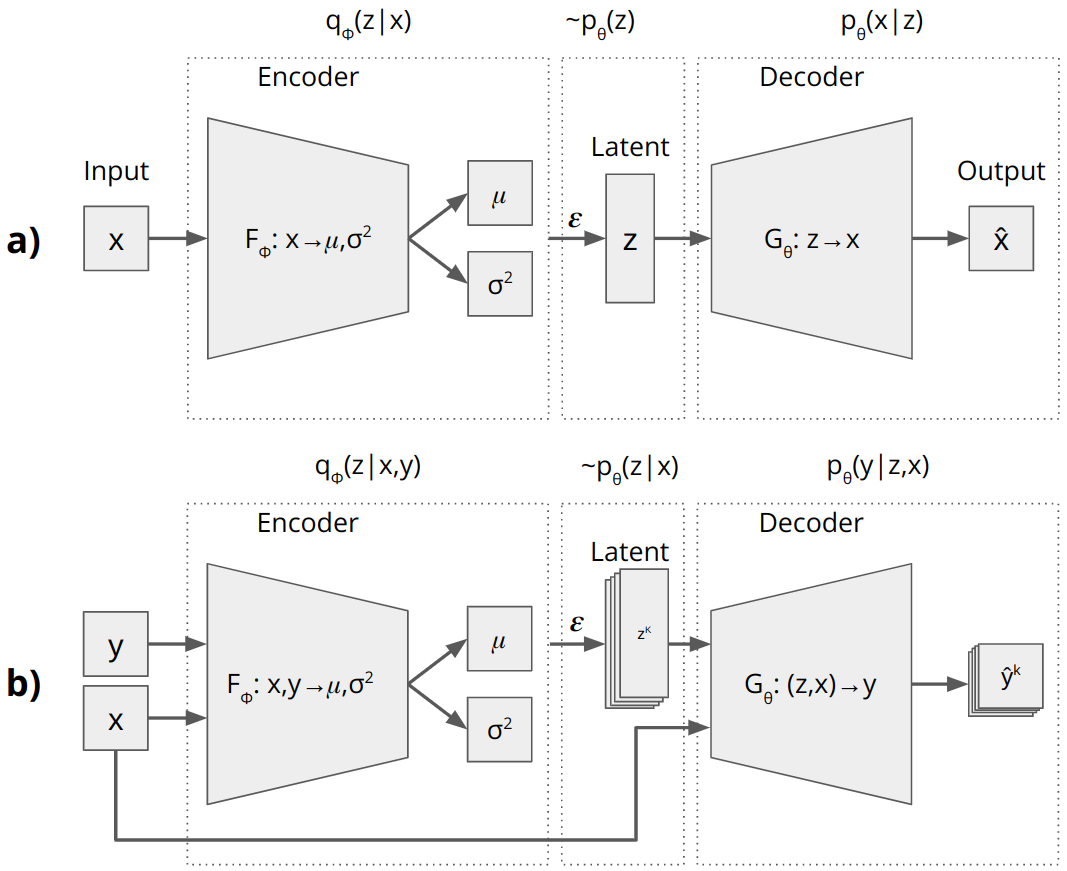
Variational inference is used to approximate a posterior distribution of a directed graphical model whose latent variables and parameters are intractable. The Variational Auto-Encoder (VAE) combines this approach with an auto-encoder framework to learn the prior distribution of a latent space, $p_{\theta}(z)$, with parameters $\theta$. The idea is that the prior distribution can then be sampled to produce a latent code, $z$, which is passed as input to the decoder to produce a sample output, $\hat{x}$. VAEs consists of two NN for the probabilistic encoding and decoding process (see Figure 1a). As the true underlying distribution of the posterior is intractable and complex, a simple parametric surrogate distribution, $q_{\Phi}(z|x)$ (such as a Gaussian), with parameters $\Phi$, is assumed to approximate the distribution and is optimized for best fit. The encoder network implicitly models the surrogate distribution, by mapping the distribution parameters, $\Phi$, during the training process. The resulting model, $q_{\Phi}(z|x)$, is referred to as the recognition model. The optimization process of the recognition model revolves around minimizing the Kullback-Leibler (KL) divergence between the posterior and surrogate distributions, and subsequently maximizing the variational lower bound (see Section 3.2). Once the latent prior distribution is learned, $z$ can be sampled via the reparameterization trick (see Section 3.3). The (probabilistic) decoder network performs a mapping of the latent code to a structured sample output for each sample, thus producing a distribution of outputs, $p_{\theta}(x|z)$.

The CVAE expands upon the framework of the VAE, by combining variational inference with a conditional directed graphical model (see Figure 1b). In the case of CVAE, the objective is to learn a prior distribution of the latent space that is conditioned on an input variable $x$ such that $p_{\theta}(z|x)$. The prior can be sampled to generate a latent code, $z$ that is passed through the decoder with $x$ to produce a sampled output, $\hat{y}$. The recognition model in this case approximates the posterior distribution of the latent space given data, $y$, conditioned on $x$ such that $p_{\theta}(z|x,y)$. The conditioning of the distributions results in a prior that is modulated, by the input variable, creating a method to control modality of the output. The recognition model $q_{\Phi}(z|x,y)$ is optimized by minimizing the KL divergence between distributions $p_{\theta}(z|x,y)$ and $q_{\Phi}(z|x,y)$. $x$ and $y$ are passed as inputs to the encoder network during training to map the parameters, $\Phi$. Latent code, $z$ is sampled from the prior distribution via, the reparametarization trick, and passed as input along with $x$ to the decoder network, producing a distribution of outputs, $p_{\theta}(y|x,z)$.

Figure 1: Overview framework of the a) VAE and b) CVAE. This figure covers both deterministic and probabilistic components for each model.

3.2 Variational Lower Bound

In Variational Inference, the main idea is to approximate the complex intractable posterior distribution $p(z|x)$, which often arises in probabilistic graphical models and other Bayesian models containing latent variables, by using a simpler and tractable distribution, $q(z|x)$. This essentially, turns the task of inference into an optimization problem in which we minimize the Kullback-Leibler (KL) divergence between the true posterior and the approximate posterior as such:

$$\begin{split}KL(q_{\phi}(z|x)||p_{\theta}(z|x))=\mathbb{E}_{q_{\phi}(z|x)}[\frac{\log q_{\phi}(z|x)}{\log p_{\theta}(z|x)}].\end{split}$$ (1)

To overcome the issue of evaluating the intractable posterior in equation 1, we rewrite the KL divergence using Bayes theorem in terms of the marginal distribution $p_{\theta}(x)$ and joint distributions $p_{\theta}(x,z)$. We can further expand the equation in terms of the marginal log-likelihood (MLL):

$$\begin{gathered}KL(q_{\phi}(z|x)||p_{\theta}(z|x))=\mathbb{E}_{q_{\phi}(z|x)}[\frac{\log q_{\phi}(z|x)p_{\theta}(x)}{\log p_{\theta}(x,z)}]\\ =\mathbb{E}_{q_{\phi}(z|x)}[\frac{\log q_{\phi}(z|x)}{\log p_{\theta}(x,z)}]+\mathbb{E}_{q_{\phi}(z|x)}[\log p_{\theta}(x)]\\ =-\mathbb{E}_{q_{\phi}(z|x)}[\frac{\log p_{\theta}(x,z)}{\log q_{\phi}(z|x)}]+\log p_{\theta}(x)\end{gathered}$$ (2)

Now we notice that the terms in equation 2 follow particular properties. First, the KL divergence between $q(z|x)$ and $p(z|x)$ is always non-negative. We also notice that the second term is the MLL, and must be a negative value since $0<p(x)<1$. Thus, we can describe the first term on the right-hand side to be a lower bound of the marginal log-likelihood, and we can define it as such:

$$\begin{multlined}\log p_{\theta}(x)\geq\mathcal{L}(\theta,\Phi)=\\ \mathbb{E}_{q_{\phi}(z|x)}[-\log q_{\phi}(z|x)+\log p_{\theta}(x,z)]\end{multlined}\log p_{\theta}(x)\geq\mathcal{L}(\theta,\Phi)=\\ \mathbb{E}_{q_{\phi}(z|x)}[-\log q_{\phi}(z|x)+\log p_{\theta}(x,z)]$$ (3)

As the variational lower bound, $\mathcal{L}(\theta,\Phi)$, increases and approaches the MLL, the KL divergence decreases, such that $KL(q_{\phi}(z|x)||p_{\theta}(z|x))=0$ when $\mathcal{L}(\theta,\Phi)=\log p_{\theta}(x)$. Thus, The optimization problem, can be evaluated as an objective function which aims to maximize the variational lower bound, which is also referred to as the Evidence Lower BOund (ELBO).

The ELBO provided in equations 3 can be further expanded in terms of the expected log likelihood as such:

$$\begin{multlined}\mathcal{L}(\theta,\Phi)=\\ -KL(q_{\phi}(z|x)||p_{\theta}(z))+\mathbb{E}_{q_{\phi}(z|x)}[p_{\theta}(x|z)]\end{multlined}\mathcal{L}(\theta,\Phi)=\\ -KL(q_{\phi}(z|x)||p_{\theta}(z))+\mathbb{E}_{q_{\phi}(z|x)}[p_{\theta}(x|z)]$$ (4)

The second term on the right-hand side of equation 4, is the expected value of the log likelihood. The first term on the right-hand side is the KL divergence between the approximate posterior and the prior distributions.

The ELBO, is a crucial aspect of optimizing the VAE and CVAE models. It serves as an objective function that needs to be maximized during the training process. The ELBO provides a balance between two competing terms: the reconstruction loss and the KL divergence. The reconstruction loss measures the difference between the original data and the data reconstructed by the model, ensuring that the model can generate accurate samples. On the other hand, the KL divergence term enforces a regularization constraint on the learned latent space, ensuring that the approximate posterior distribution remains close to the true prior distribution.

For the CVAE, the ELBO is slightly modified to account for the conditioning on the input observation variable $x$ and the reconstruction of data $y$:

$$\begin{multlined}\mathcal{L}_{CVAE}(\theta,\Phi)=\\ -KL(q_{\phi}(z|x,y)||p_{\theta}(z|x))+\mathbb{E}_{q_{\phi}(z|x,y)}[p_{\theta}(y|x,z)]\end{multlined}\mathcal{L}_{CVAE}(\theta,\Phi)=\\ -KL(q_{\phi}(z|x,y)||p_{\theta}(z|x))+\mathbb{E}_{q_{\phi}(z|x,y)}[p_{\theta}(y|x,z)]$$ (5)

In equation 5, the reconstruction loss term is adapted to include the conditioning on $x$, and the KL divergence term now measures the difference between the approximate posterior $q_{\Phi}(z|x,y)$ and the conditional prior $p_{\theta}(z|x)$. The optimization process of the CVAE revolves around maximizing this ELBO, resulting in an improved representation of the latent space and allowing for the generation of diverse and controlled outputs.

3.3 Reparametrization Trick

When modeling the recognition model implicitly by encoding the distribution parameters, the sampling step introduces non-differentiable operations that hinder the optimization process. In the context of VAEs, it is essential to have a differentiable method for generating samples from the approximate posterior distribution $q_{\Phi}(z|x)$. The reparameterization trick, proposed by Kingma et al. [10], addresses the issue of non-differentiability in the latent space sampling step. This technique enables back propagation, an important algorithm for gradient-based optimization, to function effectively despite the stochasticity in the latent variable sampling process.

The reparameterization trick introduces an auxiliary noise variable, $\epsilon$, and reformulates the latent variable as a deterministic transformation. The noise variable is independent of the model parameters and input data with a standard normal distribution, i.e., $\epsilon\sim\mathcal{N}(0,I)$. This reformulation allows gradients to flow through the deterministic portion of the model, bypassing the random component. Consequently, this technique facilitates efficient gradient estimation, stabilizes the training process, and leads to improved convergence properties.

The deterministic functional takes on the form, $z=g_{\Phi}(x,\epsilon),\epsilon\sim N(0,I)$, with parameters, $\Phi$, obtained from the encoder, typically taken as the parameters of a Gaussian distribution as such:

$$\mu,\sigma^{2}=f_{enc}(x;\Phi)$$ (6)

In the case of CVAEs, the reparameterization trick is applied similarly, but the encoder network is conditioned on both the input observation variable $x$ and the data to be reconstructed $y$:

$$\mu,\sigma^{2}=f_{enc}(x,y;\Phi)$$ (7)

The reparameterized latent variable for the CVAE is expressed as a deterministic transformation of the auxiliary variable, $z=g_{\Phi}(x,y,\epsilon)$. One such transformation, $g_{\Phi}(.)$, is given as:

$$z=\mu+\sigma\odot\epsilon,z\sim q_{\Phi}(z|x,y),\epsilon\sim N(0,I),$$ (8)

The optimization process for the CVAE, like the VAE, centers around maximizing the ELBO, as depicted in equation 5. By employing the reparameterization trick during the CVAE training process, the model is able to learn a more refined representation of the latent space, enabling the generation of diverse and controlled outputs based on the input observation variable $x$.

4 Method

The Conditional Variational Auto-Encoder (CVAE) introduced in [16] was implemented for the task of image segmentation in a generative framework. As such, the authors condition their model on images as their input, $x$. This CVAE implementation is able to outperform equivalent deterministic methods, however, the task of image-to-image translation is often a transformation from one high dimensional space to another high dimensional space. This makes it easier for models to maintain spatial and structural information shared by the input and output image. In this paper we evaluate a CVAE approach for the task of image synthesis from attributes, which performs a transformation from a low dimensional space to a high dimensional output space, specifically, text to images. This task is challenging as the generative network must construct structures that are not apparent from the low dimensional variables. In this section, we present a CVAE implementation and performance enhancing methods for the task of attribute-to-image synthesis.

4.1 Model Architecture

Our model follows a standard CNN-CVAE architecture which consists of an encoder, a decoder, and a reparameterization step that samples the recognition model (see Figure 2). The model is implemented in PyTorch [14] and the main components of the CVAE model are described below.

Figure 2: Overview of our CVAE architecture’s training and sampling pipeline

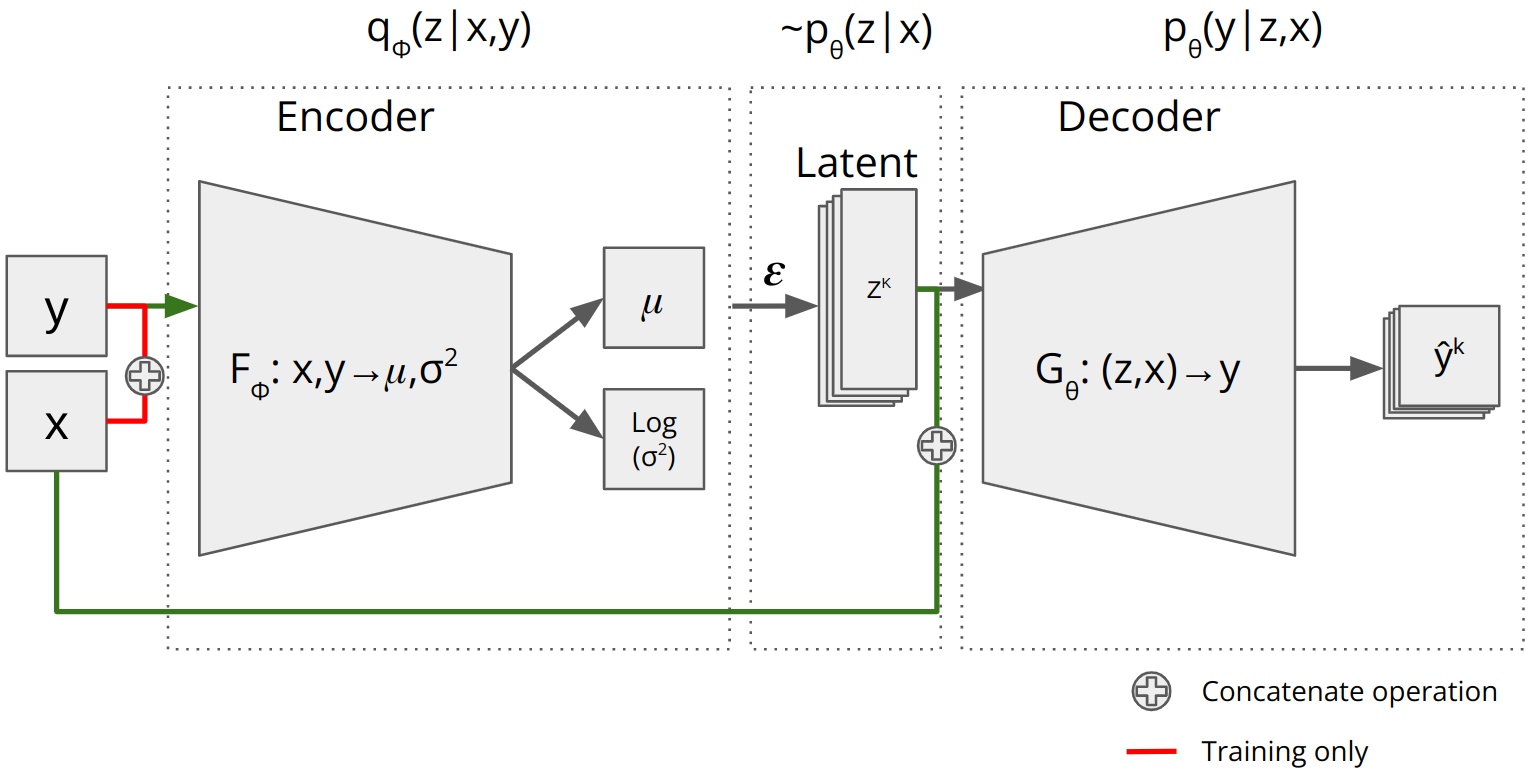
Encoder The encoder is a convolutional neural network (CNN) that takes both the training image $y$ and the conditioning variable $x$ as inputs. The conditioning variable $x$ is a one-hot-encoded tensor obtained from a list of string type attributes that correspond to training image, $y$. $x$ is reshaped and tiled to match the spatial dimensions of the training image, and then concatenated along the channel axis. The encoder processes the concatenated input through two convolutional layers, each followed by a ReLU activation function and max-pooling operation. The output is then flattened and passed through two fully connected Neural Network layers to obtain the mean $\mu$ and the log-variance $\log\sigma^{2}$ of the latent space. Encoding the log-variance provides a more stable, unconstrained optimization landscape and simplifies the loss function’s gradients, making it easier for the model to learn and optimize.

Reparameterization The reparameterization step is responsible for generating samples of latent code, $z$ from the approximate posterior distribution $q_{\Phi}(z|x)$. It takes the mean $\mu$ and the log-variance $\log\sigma^{2}$ as inputs, and applies the reparameterization trick. The log-variance is first transformed into standard deviation, and an auxiliary noise variable $\epsilon$ is sampled from a standard normal distribution, $N(0,I)$. The latent variable $z$ is then computed as $z=\mu+\sigma\odot\epsilon$.

Decoder The decoder is a CNN that takes the latent variable $z$ and the conditioning variable $x$ as inputs. The conditioning variable $x$ is reshaped and concatenated with the latent variable $z$. The combined tensor is passed through a fully connected layer NN, and then reshaped to match the spatial dimensions required for the transposed convolutional layers. The decoder processes the input through two transposed convolutional layers, each followed by a ReLU activation function, except for the final layer, which uses a Sigmoid activation to generate the output image, $\hat{y}$.

Weight Initialization The weights of the model are initialized using the Kaiming normal initialization, which is well-suited for ReLU activation functions [5]. This initialization method is based on the insight that, in deep networks, it is important to maintain the variance of the activations and gradients across layers during both forward and backward passes. This helps in preventing vanishing or exploding gradients and speeds up the training process. The biases are further initialized to zero.

The network architecture is kept shallow with only two convolutional layers and one linear layer for both the encoder and decoder. The first reason for this is for computational efficiency. Keeping the network shallow allows the training process to be faster and requires less computational resources, which is particularly important when working with large image datasets. Furthermore, using a shallow network helps avoid the vanishing gradient problem. The second reason for keeping the network architecture shallow is to prevent overfitting. Since the number of trainable parameters in a network increases with the number of layers, a deep network can be more prone to overfitting on the training data. Since one of the problems associated, with image synthesis with VAE’s is the overfitting to training images, and overall bad generalization, it is import to help our model generalize in the unknown latent space.

It is also important to note that using a shallow network may not be able to capture complex relationships between features in the data and may not perform as well as a deeper network architecture. Therefore, the decision to use a shallow or deep network is based on the specific task on the datasets (see Section 5) and the available computational resources(see Section 5.4).

4.2 Loss function

The optimization process for the CVAE revolves around maximizing the variational lower bound with the formulation presented in equation 5. In order to achieve this, the loss function used for training is a combination of the reconstruction loss and the KL-divergence loss. The reconstruction loss is calculated as the mean squared error (MSE) between the output image, $\hat{y}$, and the original training image, $y$. The KL-divergence loss is calculated using the mean $\mu$ and the log-variance $\log\sigma^{2}$ produced by the encoder. The total loss is the sum of these two components. A weighted term, $\beta$, is introduced as a tunable parameter for controlling which term to place more importance. $\beta<0.5$ corresponds to more importance placed on the reconstruction loss to the overall loss function, whereas $\beta>0.5$ corresponds to more importance placed on the regularizing term.

$$\mathcal{L}_{CVAE}=(1-\beta)\cdot\text{MSE}(\hat{y},y)+\beta\cdot\text{KL}(\mu,\log\sigma^{2})$$ (9)

where $\text{MSE}(\hat{y},y)$ represents the mean squared error between the output and target images, and $\text{KL}(\mu,\log\sigma^{2})$ is the KL-divergence term given by:

$$\text{KL}(\mu,\log\sigma^{2})=-\frac{1}{2}\sum_{i=1}^{n}\left(1+\log\sigma_{i}^{2}-\mu_{i}^{2}-\text{exp}(\log\sigma_{i}^{2})\right)$$ (10)

Where, $n$ is the number of elements in the latent vector.

The CVAE model is trained using the Adam optimizer [8], a gradient-based optimization, with back propagation enabled by the reparameterization trick. The model architecture and implementation are designed to provide an effective and efficient way of learning a rich and diverse representation of the data in the latent space, while also enabling the generation of controlled and high-quality outputs.

5 Experiments

5.1 CelebFaces Attributes Dataset

The CelebFaces Attributes Dataset (CelebA) [12] is a large-scale face attributes dataset containing more than 200,000 celebrity images, each annotated with 40 binary attribute labels, such as gender, age, and hair color. The dataset consists of diverse images of various celebrities, making it a popular choice for facial attribute recognition and generation tasks. The images in CelebA are provided in a resolution of 178x218 pixels. These images are collected from various sources from the internet and do not have consistent background and are thus considered ”in-the-wild”. In our study, we employ the CelebA dataset to train our CVAE model on the task of image synthesis from attributes, focusing on generating images based on the provided facial attributes. No data augmentation or preprocessing is performed on these images for this experiment.

5.2 Caltech-UCSD Birds-200-2011

The Caltech-UCSD Birds-200-2011 (CUB-200-2011) dataset [18] is a widely used dataset for fine-grained visual categorization. It consists of 11,788 images of 200 different bird species. Each image is annotated with a bounding box, part locations, and 312 binary attribute labels, making it suitable for various computer vision tasks such as object detection, segmentation, and fine-grained classification. The dataset is split into a training set containing 5,994 images and a test set containing 5,794 images. In our experiments, we utilize the bird images and their corresponding attribute labels to train and evaluate our CVAE model. In this experiment bird species are treated as additional attributes, and are converted to into one-hot-encoding and concatenated with the rest of the binary attributes. Images are taken from the internet and are considered to be ”in-the-wild”. Sizes of each image vary and are resized to 244x244px, before feeding through our models.

5.3 Effect of $\beta$ on Regularization

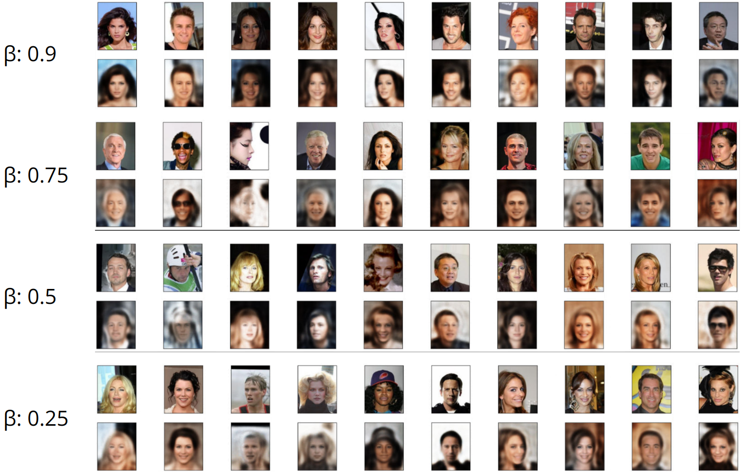
To investigate the impact of the $\beta$ parameter on the balance between reconstruction and regularization, we trained the CVAE model using different values of $\beta$ ranging from 0.25 to 0.9. The values were chosen to provide insights on the behavior of the model with varying levels of importance assigned to the KL-divergence vs reconstruction terms in the loss function. The $\beta$ values tested were 0.25, 0.5, 0.75, and 0.9. The CVAE model was trained separately for each $\beta$ value, keeping all other hyperparameters consistent across the experiments. The learning rate, batch size, and number of epochs were kept constant for a fair comparison. The CVAE loss function was used to compute the balance between reconstruction and regularization. After training the model with different $\beta$ values, the quality of the reconstructions, the latent space representations, and the generalization capability of the model were analyzed using the following evaluation metrics:

Reconstruction Error The reconstruction error for each $\beta$ value is computed by measuring the mean squared error (MSE) between the input images and the reconstructed images. This metric helps in understanding how well the CVAE model can reproduce the input data.

Generalization and Disentanglement the latent space is evaluated by analyzing the relationship between the latent variables and the semantic attributes of the input data. Generalization of the model is assessed by observing its performance on unseen data. This was achieved by evaluating the attributes present in images with varying attributes, as well as, assessing the quality of image generated. A more disentangled latent space would lead to better interpretability and generalization.

5.4 Hardware and Software Setup

The experiments in this study were conducted using a workstation equipped with an NVIDIA GeForce RTX 2080 Ti GPU, an AMD Ryzen 7 2700X Eight-Core Processor, and 64 GB of RAM. The operating system installed on the workstation was Ubuntu 22.04.2 LTS. For the implementation of the model and conducting experiments, we utilized several software libraries. PyTorch version 2.0, compiled with CUDA 11.7 for GPU acceleration, was employed for the deep learning framework. Additionally, NumPy was used for numerical computation and data manipulation, while Matplotlib was utilized for data visualization and generating plots.

6 Results and Discussion

6.1 Synthesized Image Assessment

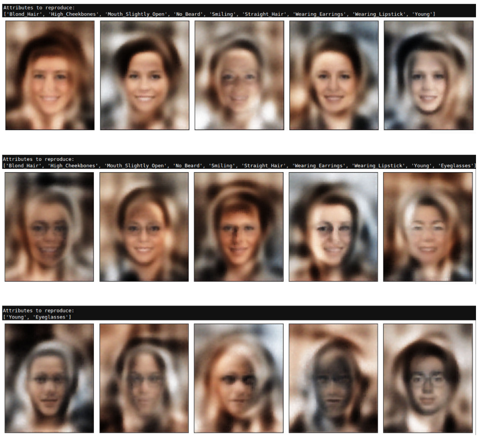
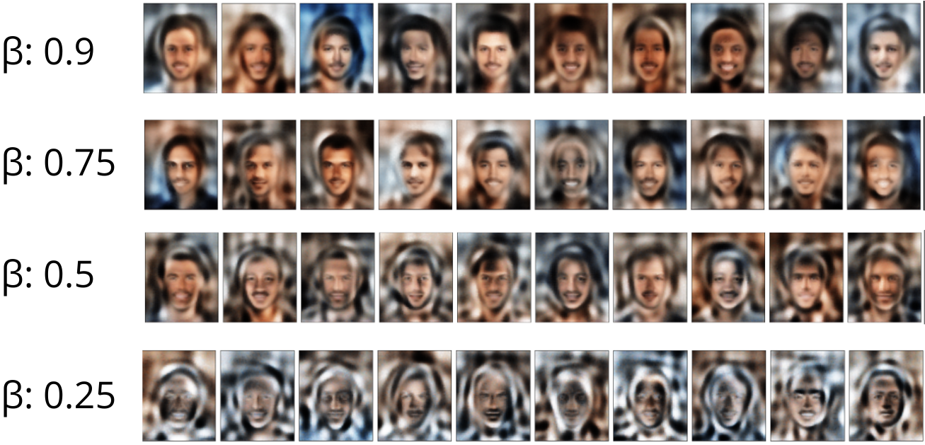
CelebA A qualitative assessment shows that our CVAE architecture is able to generate structured output that resemble human faces with the desired attributes. In general, facial structures are constructed from a set of string based attributes and a randomly sampled latent code, without any other information about spatial interactions. We notice that faces from the training data are typically found towards the center of the image and all faces tend to hold similarities in spatial structures. For example, a nose, two eyes, a mouth and general shape tend to have spatial consistency. More variability is introduced as we move further from the center, attributes such as hairstyles, outfit and background, change significantly and often are not captured in the list of attributes. This is reflected in the generated images, as facial structures are captured in higher detail in the center, and as we move further out, structures tend to be more ambiguous and blurry. To test the robustness of the model, random attributes were selected, added and removed to measure the extent of the samples generated, and indeed fairly good samples are generated for all cases (see Figure 5).

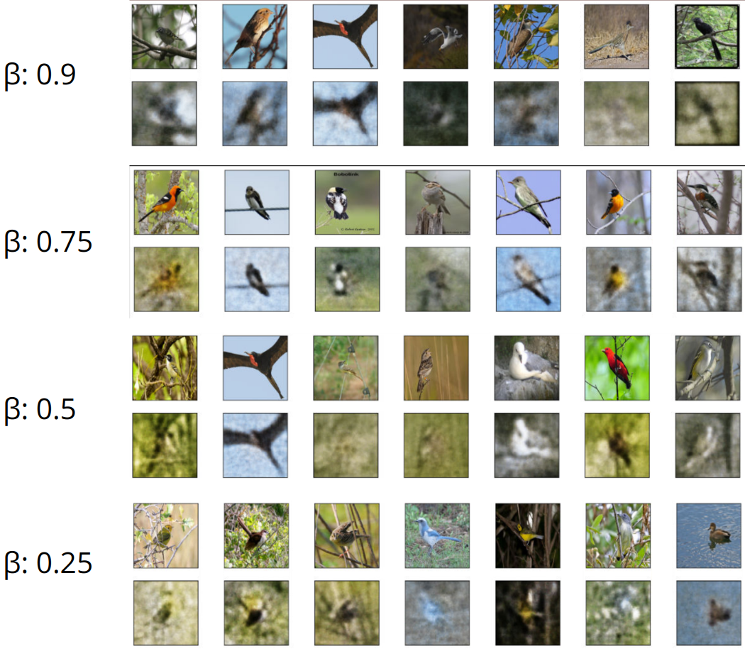
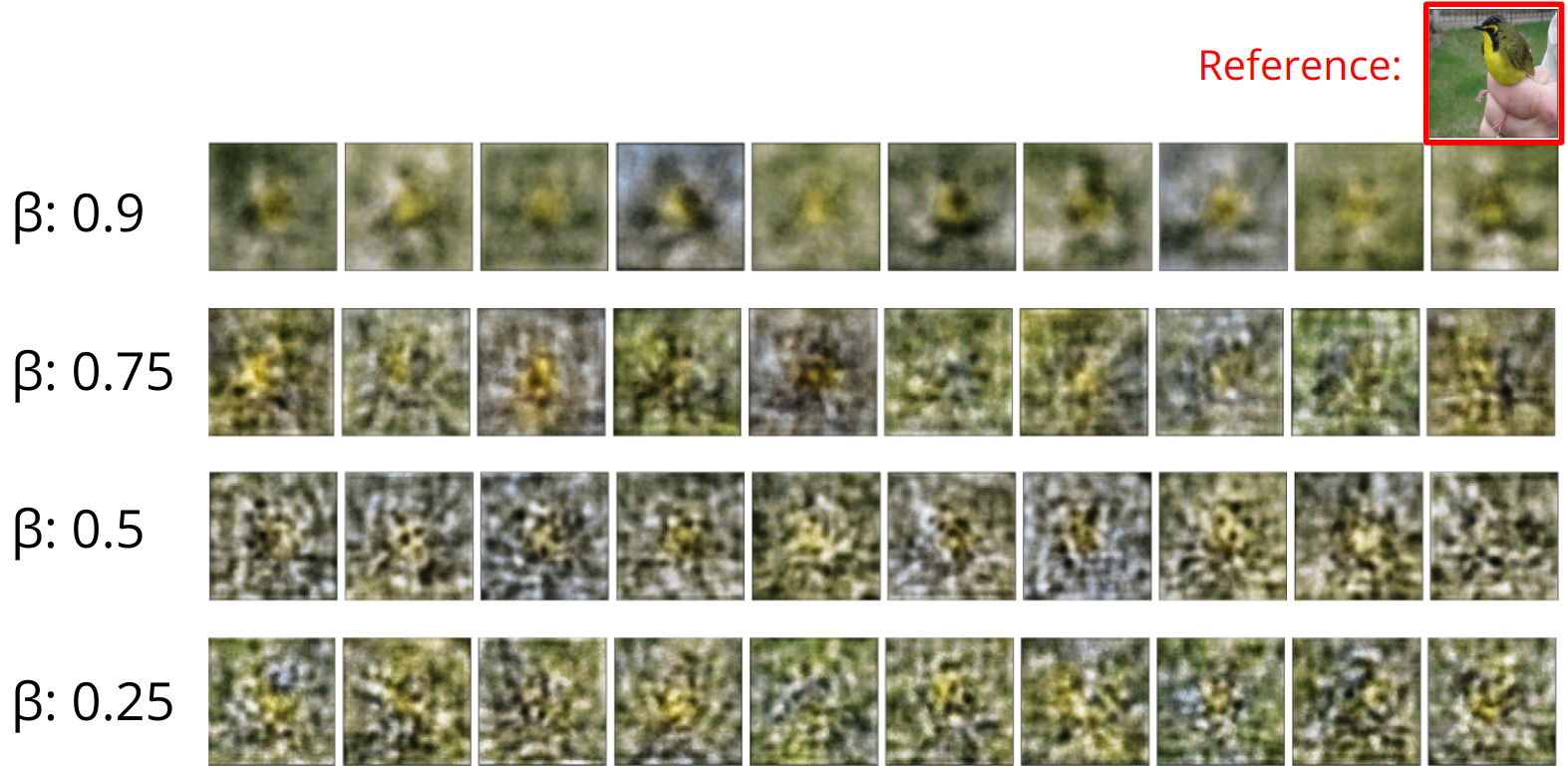
CUB-200-2011 A qualitative assessment of the samples show that we were not able to generate highly detailed structured images of birds. However, we notice that the model tries to recreate generalities about the attributes that birds hold. If we examine in Figure 3(b) our model is able to generally, produce the color palette of the bird with desired attributes. If we further examine the first row, as we increase regularization, more structures seem to be apparent, albeit blurry. This is most likely due to the variability in structures within the images, as well as sparsity of training images with the held attributes.

(a) CelebA

(b) CUB-200-2011

Figure 3: Samples generated from model trained on $\beta$ values ranging from 0.25 to 0.9

6.2 Reconstruction vs Regularization

The intuition behind modulating the regularization and reconstruction terms is to penalize overfitting of the recognition model to the structures of the training data, while maintaining the structural learning process. We notice in Figures 3(a) and 3(b) that low $\beta$ value, result in high frequency ambiguities (in celebA) and artifacts (in cub-200-2011) when generating samples. While we are able to achieve very accurate reconstructions of the training images in both datasets, the objective is to synthesize a variety of generalized faces that hold those attributes. Thus, querying the generative network trained on a low $\beta$ value results in uncertain and ambiguous structures in the output image. As we increase $\beta$, however, the regularization term is favored, resulting in much more natural generation of the faces, and smoother and structurally sound images of birds. In Table 1 we observe that $\beta=0.25$ achieves the lowest mean squared error, which corresponds to accurate reconstructions during training (see Figure 4(a)). However, it is apparent that sampling from selected attributes and a random latent code, the network trained on $\beta=0.25$, performs the worst, with unrealistic synthesized images, as show in the last row of Figure 3(a). This is especially apparent in the CUB-200-2011 dataset, in Figure 4(b), as the model does a very good job at reconstructing the training image, however it fails to generate any significant structures during sampling. Since the task of image synthesis is to generate variations of structured outputs from the same attributes, a higher $\beta$ value is desired, as it helps the model avoid overfitting and puts more significance in achieving a regularized solution that keeps our recognition model close the prior distributions of the latent space.

	CelebA		CUB-200-2011
$\beta$	MSE	KL	MSE	KL
0.9	82787	9515	20129	482
0.75	81157	10033	13446	2315
0.5	73137	15845	13256	3677
0.25	70444	27107	12093	4957

Table 1: Mean Squared Error and KL losses for models trained on $\beta$ ranging from 0.25 to 0.9

7 Conclusion

In this paper, we have demonstrated the effectiveness of the Conditional Variational Auto-Encoder as a powerful generative model for constructing high-dimensional structured outputs from low-dimensional attributes. This framework enables the generation of disentangled samples of images with numerous variations of the same attributes, highlighting its potential for diverse applications in image synthesis. Our study further reveals that a higher weight placed on the regularization term of the loss function of the CVAE during training is favored in image synthesis tasks. This is because the primary objective is not to learn accurate reconstructions but rather to capture the variations in the latent space effectively. However, challenges remain in capturing high-frequency variabilities in sparse image datasets. Despite these limitations, our CVAE model still demonstrates the ability to generate meaningful representations in a controlled manner. Image synthesis from text is often challenging, as spatial information is not directly available to the model. The CVAE framework proves its versatility and adaptability to such complex scenarios.

Finally, improvements to data pre-processing and data augmentation techniques can significantly improve results. As a fully supervised method, CVAEs are completely dependent on the quality of the data it is trained on. As such various challenges arise, especially when dealing with uncertainties and implicit biases. Further research should be conducted in this area to improve utilization of deep Condition Generative Models, such as the CVAE.

(a) CelebA

(b) CUB-200-2011

Figure 4: Reconstructed images generated during training from model with $\beta$ values ranging from 0.25 to 0.9. For each $\beta$ the upper row is the Ground Truth image and the bottom is the reconstructed image

Figure 5: Samples generated to demonstrate robustness of the CVAE mdoel

References

- [1] Xi Chen, Yan Duan, Rein Houthooft, John Schulman, Ilya Sutskever, and Pieter Abbeel. Infogan: Interpretable representation learning by information maximizing generative adversarial nets. In Advances in Neural Information Processing Systems, pages 2172–2180, 2016.
- [2] Laurent Dinh, David Krueger, and Yoshua Bengio. Nice: Non-linear independent components estimation. In arXiv preprint arXiv:1410.8516, 2014.
- [3] Laurent Dinh, Jascha Sohl-Dickstein, and Samy Bengio. Density estimation using real nvp. In arXiv preprint arXiv:1605.08803, 2016.
- [4] Ian Goodfellow, Jean Pouget-Abadie, Mehdi Mirza, Bing Xu, David Warde-Farley, Sherjil Ozair, Aaron Courville, and Yoshua Bengio. Generative adversarial nets. In Advances in neural information processing systems, pages 2672–2680, 2014.
- [5] Kaiming He, Xiangyu Zhang, Shaoqing Ren, and Jian Sun. Delving deep into rectifiers: Surpassing human-level performance on imagenet classification. In Proceedings of the IEEE International Conference on Computer Vision, pages 1026–1034, 2015.
- [6] Irina Higgins, Loic Matthey, Arka Pal, Christopher Burgess, Xavier Glorot, Matthew Botvinick, Shakir Mohamed, and Alexander Lerchner. beta-vae: Learning basic visual concepts with a constrained variational framework. In International Conference on Learning Representations, 2017.
- [7] Jonathan Ho, Xi Chen, Aravind Srinivas, Yan Duan, Pieter Abbeel, and Tianqi Chen. Denoising diffusion probabilistic models. arXiv preprint arXiv:2006.11239, 2020.
- [8] Diederik P Kingma and Jimmy Ba. Adam: A method for stochastic optimization. arXiv preprint arXiv:1412.6980, 2014.
- [9] Diederik P Kingma and Prafulla Dhariwal. Glow: Generative flow with invertible 1x1 convolutions. In Advances in Neural Information Processing Systems, pages 10215–10224, 2018.
- [10] Diederik P Kingma and Max Welling. Auto-encoding variational bayes. arXiv preprint arXiv:1312.6114, 2013.
- [11] Guillaume Lample, Neil Zeghidour, Nicolas Usunier, Antoine Bordes, Gabriel Synnaeve, and Yann Pietquin. Fader networks: Manipulating images by sliding attributes. In Advances in Neural Information Processing Systems, pages 5967–5976, 2017.
- [12] Ziwei Liu, Ping Luo, Xiaogang Wang, and Xiaoou Tang. Deep learning face attributes in the wild. In Proceedings of International Conference on Computer Vision (ICCV), December 2015.
- [13] Mehdi Mirza and Simon Osindero. Conditional generative adversarial nets. In arXiv preprint arXiv:1411.1784, 2014.
- [14] Adam Paszke, Sam Gross, Francisco Massa, Adam Lerer, James Bradbury, Gregory Chanan, Trevor Killeen, Zeming Lin, Natalia Gimelshein, Luca Antiga, Alban Desmaison, Andreas Kopf, Edward Yang, Zachary DeVito, Martin Raison, Alykhan Tejani, Sasank Chilamkurthy, Benoit Steiner, Lu Fang, Junjie Bai, and Soumith Chintala. Pytorch: An imperative style, high-performance deep learning library, 2019.
- [15] Danilo Jimenez Rezende and Shakir Mohamed. Variational inference with normalizing flows. arXiv preprint arXiv:1505.05770, 2015.
- [16] Kihyuk Sohn, Honglak Lee, and Xinchen Yan. Learning structured output representation using deep conditional generative models. In C. Cortes, N. Lawrence, D. Lee, M. Sugiyama, and R. Garnett, editors, Advances in Neural Information Processing Systems, volume 28. Curran Associates, Inc., 2015.
- [17] Yang Song and Stefano Ermon. Score-based generative modeling through stochastic differential equations. arXiv preprint arXiv:2102.07574, 2021.
- [18] C. Wah, S. Branson, P. Welinder, P. Perona, and S. Belongie. Caltech-ucsd birds-200-2011 (cub-200-2011). Technical Report CNS-TR-2011-001, California Institute of Technology, 2011.