Color confinement due to topological defects
—restoration of residual gauge symmetries—

Abstract

The local gauge symmetry remaining even after imposing a gauge fixing condition is called the residual local gauge symmetry, which is spontaneously broken in the perturbative vacuum, and is expected to be restored in the true confining vacuum. Indeed, the criterion for restoring a special choice of the residual gauge symmetry was shown to be equivalent to the Kugo-Ojima color confinement criterion in the Lorenz gauge. In the previous paper, we demonstrated that such restoration can occur even in the Maximal Abelian gauge due to topological defects. However, it was later found that the topological defects introduced in the previous paper give an infinite Euclidean action and hence do not contribute to the path integral. In this paper, therefore, we reexamine modified topological defects giving a finite Euclidean action to contribute to the path integral. We show the restoration of the residual local gauge symmetry in the Maximal Abelian gauge due to such a class of topological defects.

1 Introduction

Color confinement is still an unsolved important problem in particle physics. Especially, quark confinement is well understood based on the dual superconducting picture where condensation of magnetic monopoles and anti-monopoles occursdual-superconductor . On the other hand, gluon confinement is not so well understood in this picture. However, a general color confinement criterion exists: If the Kugo-Ojima (KO) criterionKO was satisfied, no particles with color charges would be observedKO-prove . The KO criterion was derived only in the Lorenz gauge and is clearly gauge-dependent. Therefore, it cannot be directly applied to the other gauge-fixing conditions.

The local gauge symmetry remaining after imposing a gauge fixing condition is called the residual local gauge symmetry. Although the residual local gauge symmetry is “spontaneously” broken in the perturbative vacuum, it is expected to be restored in the true confining vacuum. The criterion for the restoration can be formulated as the condition for disappearance of the massless Nambu-Goldstone (NG) pole associated with the “spontaneous symmetry breaking” of the residual gauge symmetry. Remarkably, the KO criterion was reproduced as a restoration condition for the residual local gauge symmetry in the Lorenz gaugeHata-method when the gauge transformation function is a linear function of the spacetime coordinate $x^{\mu}$.

The restoration condition for the residual local gauge symmetry can also be extended to more general gauge transformations, including those involving topological configurations. In the previous paperKondo-Fukushima , indeed we introduced topological defects to demonstrate in the configuration space that it is possible to satisfy the restoration condition even in the Maximal Abelian gauge. Hence, it enables us to understand color confinement from the view point of restoration of the residual gauge symmetry due to topological defects. However, it turns out that the topological configurations introduced in the previous paper give an infinite Euclidean action and do not contribute to the path integral. In this paper, therefore, we reexamine the restoration condition using topological defects giving a finite Euclidean action which contribute to the path integral. Additionally, we focus on the momentum space to clarify what types of divergence arise in the calculation of the restoration condition, and we propose a physical picture for restoration of the residual local gauge symmetry.

This paper is organized as follows. In Sec. 2, we remember the relation between the restoration condition for gauge symmetry in the Lorenz gauge and the Kugo-Ojima color confinement criterion. In Sec. 3, we present the restoration condition for general residual gauge symmetry in the Maximal Abelian gauge. In Sec. 4, we introduce a concrete topological configuration that contribute to the path integral and reconsider the restoration condition. The final section is devoted to conclusion and discussion. The details of the calculations are given in Appendices A, B, C.

2 Residual local gauge symmetry restoration in the Lorenz gauge

We consider the Yang-Mills theory coupled to the matter field in the non-compact formulation where the Yang-Mills gauge field $\mathscr{A}_{\mu}(x)$ is defined as the Lie algebra valued field $\mathscr{A}_{\mu}(x)=\mathscr{A}_{\mu}^{A}(x)T_{A}$ with the generators $T_{A}$ ($A=1,\cdots,\text{dim}SU(N)=N^{2}-1$) of the Lie algebra $su(N)$ for the $SU(N)$ gauge group. The total Lagrangian density is given by

$$\mathscr{L}=\mathscr{L}_{\text{inv}}+\mathscr{L}_{\text{GF+FP}}.$$ (1)

The first term $\mathscr{L}_{\text{inv}}$ is the gauge-invariant part given by

$$\mathscr{L}_{\text{inv}}=-\frac{1}{4}\mathscr{F}_{\mu\nu}\cdot\mathscr{F}^{\mu\nu}+\mathscr{L}_{\text{matter}}(\varphi,D_{\mu}\varphi),$$ (2)

with the Lie algebra valued field strength $\mathscr{F}_{\mu\nu}$ of the gauge field $\mathscr{A}_{\mu}$ defined by $\mathscr{F}_{\mu\nu}:=\partial_{\mu}\mathscr{A}_{\nu}-\partial_{\nu}\mathscr{A}_{\mu}+g\mathscr{A}_{\mu}\times\mathscr{A}_{\nu}=-\mathscr{F}_{\nu\mu}$ and the covariant derivative $D_{\mu}\varphi$ of the matter field $\varphi$ defined by $D_{\mu}\varphi:=\partial_{\mu}\varphi-ig\mathscr{A}_{\mu}\varphi$.

The second term $\mathscr{L}_{\text{GF+FP}}$ is the sum of the gauge fixing (GF) term $\mathscr{L}_{\text{GF}}$ including the Nakanishi-Lautrup (NL) field $\mathscr{B}(x)$ as the Lagrange multiplier field to incorporate the gauge fixing condition to be specified later, and the associated Faddeev-Popov (FP) ghost term $\mathscr{L}_{\text{FP}}$ including the ghost field $\mathscr{C}(x)$ and the antighost field $\bar{\mathscr{C}}(x)$. Here $\mathscr{B}(x),\mathscr{C}(x),\bar{\mathscr{C}}(x)$ are also Lie algebra valued fields. In what follows we use the notation for the Lie-algebra valued quantities $\mathscr{A},\mathscr{B}$: $(\mathscr{A}\times\mathscr{B})^{A}=f^{ABC}\mathscr{A}^{B}\mathscr{B}^{C}$ with the structure constant $f^{ABC}$ for the $su(N)$ Lie algebra with the indices $A,B,C=1,\cdots,\text{dim}SU(N)=N^{2}-1$.

First, we consider the Lorenz gauge fixing given by the usual local condition:

$$\partial^{\mu}\mathscr{A}_{\mu}(x)=0.$$ (3)

Even after imposing the gauge fixing condition which breaks the gauge symmetry, the non-compact gauge theory with the total Lagrangian density $\mathscr{L}$ has the Becchi-Rouet-Store-Tyutin (BRST) symmetry. Using the nilpotent BRST transformation $\delta_{\text{B}}$, indeed, the associated GF+FP term is written in the BRST exact form:

$$\mathscr{L}_{GF+FP}=-i\delta_{\text{B}}\left\{\bar{\mathscr{C}}^{A}\left(\partial^{\mu}\mathscr{A}_{\mu}+\frac{\alpha}{2}\mathscr{B}\right)^{A}\right\},$$ (4)

where $\alpha$ is the gauge-fixing parameter.

Let $\mathcal{V}_{\text{phys}}$ be the physical subspace of the total state space $\mathcal{V}$ with an indefinite metric defined using the nilpotent BRST charge $Q_{B}$ as the generator of the BRST transformation:

$$\mathscr{V}_{\text{phys}}=\{\ket{\text{phys}}\in\mathcal{V};\ Q_{B}\ket{\text{phys}}=0\}\subset\mathcal{V}.$$ (5)

Kugo and Ojima KO found: if the following condition called the Kugo-Ojima color confinement criterion in the Lorenz gauge is satisfied:

$$\lim_{p^{2}\rightarrow\ 0}u^{AB}(p^{2})=-\delta^{AB}\ \Leftrightarrow\ 0=\lim_{p^{2}\rightarrow\ 0}[\delta^{AB}+u^{AB}(p^{2})],$$ (6)

for the function $u^{AB}$ called the Kugo-Ojima function defined by

$$u^{AB}(p^{2})\left(g_{\mu\nu}-\frac{p_{\mu}p_{\nu}}{p^{2}}\right)=\int d^{D}x\ e^{ip(x-y)}\braket{0}{\text{T}[(\mathscr{D}_{\mu}\mathscr{C})^{A}(x)g(\mathscr{A}_{\mu}\times\bar{\mathscr{C}})^{B}(y)]}{0},$$ (7)

then the color charge operator $Q^{A}$ is well defined, namely, the color symmetry is not spontaneously broken and $Q^{A}$ vanishes for any physical state $\Phi,\Psi\in\mathcal{V}_{\text{phys}}$:

$$\braket{\Phi}{Q^{A}}{\Psi}=0,\ \Phi,\Psi\in\mathcal{V}_{\text{phys}}.$$ (8)

This means that all colored particles cannot be observed and only color singlet particles can be observed, because the BRS singlets as physical particles are all color singlets, while colored particles belong to the BRS quartet representation with zero-norm combinations.

To discuss the restoration of the residual gauge symmetry, we introduce the generalized local gauge transformation with a Lie-algebra valued transformation function $\omega(x)=\omega^{A}(x)T_{A}$:

$$\delta^{\omega}\mathscr{A}_{\mu}(x) =\mathscr{D}_{\mu}\omega(x):=\partial_{\mu}\omega(x)+g\mathscr{A}_{\mu}\times\omega(x),$$

$$\delta^{\omega}\varphi(x) =ig\omega(x)\varphi(x),$$ (9)

together with

$$\delta^{\omega}\mathscr{B}(x) =g\mathscr{B}(x)\times\omega(x),$$

$$\delta^{\omega}\mathscr{C}(x) =g\mathscr{C}(x)\times\omega(x),$$

$$\delta^{\omega}\bar{\mathscr{C}}(x) =g\bar{\mathscr{C}}(x)\times\omega(x),$$ (10)

which are just given by localizing the global transformation. In order to identify this transformation with the residual local gauge symmetry of the Lorenz gauge, the transformation function $\omega^{A}(x)$ should satisfy the Laplace equation almost everywhere:

$$\partial_{\mu}\partial^{\mu}\omega^{A}(x)=0.$$ (11)

According to our previous paperKondo-Fukushima , the general condition for restoration of a residual gauge symmetry (9), (10) satisfying (11) is given by

$$0=\lim_{p^{2}\rightarrow\ 0}\int d^{D}x\ e^{ipx}\partial^{\mu}\omega(x)\left(g_{\mu\nu}-\frac{\partial_{\mu}^{x}\partial_{\nu}^{x}}{\partial_{x}^{2}}\right)[\delta^{AB}\delta^{(D)}(x-y)+u^{AB}(x-y)],$$ (12)

where $u^{AB}$ is the Kugo-Ojima function in the configuration space defined by

$$\braket{0}{\text{T}(\mathscr{D}_{\mu}{\mathscr{C}})^{A}(x)(g\mathscr{A}_{\nu}\times\bar{\mathscr{C}})^{B}(y)}{0}=\left(g_{\mu\nu}-\frac{\partial_{\mu}^{x}\partial_{\nu}^{x}}{\partial_{x}^{2}}\right)u^{AB}(x-y)$$ (13)

If the gauge transformation function $\omega(x)$ takes a non-compact form: $\omega(x)$ is linear to $x$:

$$\omega(x)=b_{\mu}x^{\mu},$$ (14)

the condition (12) is reduced to the Kugo-Ojima color confinement criterion (6). In the Lorenz gauge, the condition for restoration of the residual local gauge symmetry is equivalent to the Kugo-Ojima color confinement criterion in the the non-compact formalism. This is a remarkable result first shown by Hata Hata-method .

In order to check whether the Kugo-Ojima criterion (6) really holds or not, the numerical simulations have been performed on the lattice Furui-Nakajima ; Sternbeck where the Kugo-Ojima function $u(p^{2})$ ($u^{AB}(p^{2})=\delta^{AB}u(p^{2})$) was measured in the Euclidean region. In order to check the KO criterion, we need the value of the KO function in the infrared limit $p^{2}\rightarrow\ 0$. Taking the limit $p^{2}\rightarrow\ 0$ needs the infinite volume lattice, which is impossible to be realized in practice. Therefore, the data $u(p^{2})$ at small but non-zero $p^{2}$ obtained on the large but finite lattice were extrapolated to $p^{2}\rightarrow 0$. In those works, it has been shown that the KO criterion is not exactly satisfied as a result of the extrapolation, although the Kugo-Ojima function $u(p^{2})$ tends to approach $-1$ as the volume of the lattice increases.

However, the simple comparison between the theoretical result for the KO criterion in the continuum non-compact formulation and the numerical result of simulations based on the lattice gauge theory is meaningless even after putting aside the extrapolation ambiguity and the finite volume effect. The examination must be done with great care as explained below.

(i) incomplete gauge fixing and the Gribov copies

In both derivations of the KO criterion mentioned above, it was assumed that the gauge fixing is achieved by the usual local gauge fixing condition $\partial_{\mu}\mathscr{A}^{\mu}=0$. Therefore, the Gribov copies were not taken into account in these derivations. In order to avoid this problem, global minimization of the gauge fixing functional is necessary. In the lattice gauge theory, the gauge fixing is in principle performed by the global minimization and therefore the results must be free from the Gribov problem (except for the lattice Gribov copies and practical limitations for time and resources)

(ii) compact formulation and including topological configurations

The lattice gauge theory is based on the compact formulation written in terms of the Lie-group valued gauge variables, while the continuum theory is based on the non-compact formulation written in terms of the Lie-algebra valued gauge potentials, although the continuum limit of the lattice gauge theory is expected to essentially reproduce the non-compact continuum theory in the scaling region. The lattice gauge theory enables to incorporate the topological configurations from the beginning. According to the lattice study, it has been confirmed that the topological configurations give the dominant contributions for quark confinement. Whereas the Kugo-Ojima result is based on the canonical operator formalism in the non-compact formulation and do not take into account the topological configurations which are usually incorporated in the path integral formalism. It is important to take into account the topological objects to bridge the gap between lattice gauge theory and continuum gauge theory. This is the very reason why we incorporate the topological configuration also in the study of color confinement.

The KO color confinement criterion was reproduced from the viewpoint of the restoration of the residual local gauge symmetry, only when the gauge-transformation $\omega(x)$ is linear to $x$, which is referred to as the non-compact case in our paper. However, the choice for $\omega(x)$ is not unique and there is no sure physical reason to choose the above linear form, since it was just chosen from the analogy in the Abelian gauge theory by the reason it is the simplest form for satisfying the Laplace equation (11) which is a condition to guarantee the residual gauge symmetry in the Lorenz gauge. Therefore, the gauge-transformation function $\omega(x)$ can take different forms other than the above specific form, which does not lead to the KO criterion. Thus we do not consider that the KO criterion is a true criterion for color confinement to be derivable as the restoration of the residual gauge symmetry even in the Lorenz gauge. Therefore, it is not a surprise to us that KO criterion is not satisfied in the results of numerical simulations on the latticeFurui-Nakajima ; Sternbeck , while the lattice results support confinement.

Moreover, the gauge-fixed lattice simulations in the last two decades have displayed the high level of sophistication on the issues. Indeed, they have given the critical reassessment of the entire confinement mechanism that has been caused as a result of the lattice simulations, at the level of the gluon and ghost propagator. In particular, a series of pivotal results Boucaud ; Bogolubsky ; Cucchieri ; Sternbeck-Smekal have dispelled the “ghost-dominance” scenario of QCD, which is the intellectual offspring of the KO formalism.

We examine the compact case $\omega(x)$ giving the topological configurations to see the effect of the topological defects to color confinement from the viewpoint of residual gauge symmetry restoration, although the Gribov problem still exists. This is motivated from the conventional wisdoms mainly obtained after the proposal of the KO criterion based on the lattice gauge theories and the other non-perturbative methods claiming that topological configurations are dominantly responsible for non-perturbative phenomena such as confinement and chiral symmetry breaking.

3 Residual local gauge symmetry restoration in the Maximal Abelian gauge

Next, we consider the Maximal Abelian (MA) gauge. To define the MA gaugeMA , we need to decompose the Lie-algebra valued quantity into its diagonal Cartan part and the remaining off-diagonal part, e.g., the gauge field $\mathscr{A}_{\mu}(x)=\mathscr{A}_{\mu}^{A}(x)T_{A}$ with the generators $T_{A}\ (A=1,\cdots,N^{2}-1)$ of the Lie algebra $su(N)$ has the decomposition:

$$\mathscr{A}_{\mu}(x)=\mathscr{A}_{\mu}^{A}(x)T_{A}=a_{\mu}^{j}(x)H_{j}+A_{\mu}^{a}(x)T_{a},$$ (15)

where $H_{j}$ are the Cartan generators and $T_{a}$ are the remaining generators of $su(N)$. In what follows, the indices $j,k,\ell,\cdots$ label the diagonal components and the indices $a,b,c,\cdots$ label the off-diagonal components. Then, the MA gauge is given by

$$(\mathscr{D}^{\mu}[a]A_{\mu}(x))^{a}:=\partial^{\mu}A_{\mu}^{a}(x)+gf^{ajb}a^{\mu j}(x)A_{\mu}^{b}(x)=0,$$ (16)

where we have used a property of the structure constant: $f^{jkA}=0$. The MA gauge is a partial gauge fixing applied to only off-diagonal components, and hence does not fix the diagonal components. Therefore, we further impose the Lorenz gauge for the diagonal components:

$$\partial^{\mu}a_{\mu}^{j}(x)=0\ (j=1,2,\cdots N-1).$$ (17)

Using the BRST transformation $\delta_{\text{B}}$, the GF+FP term for the gauge-fixing condition (16) and (17) with the respective gauge-fixing parameter $\alpha$ and $\beta$ is given by

$$\mathscr{L}_{GF+FP}=-i\delta_{\text{B}}\left\{\bar{C}^{a}\left(\mathscr{D}^{\mu}[a]A_{\mu}+\frac{\alpha}{2}B\right)^{a}\right\}-i\delta_{\text{B}}\left\{\bar{c}^{j}\left(\partial^{\mu}a_{\mu}+\frac{\beta}{2}b\right)^{j}\right\}.$$ (18)

The change of the Lagrangian density under the generalized local gauge transformation (9) and (10) is given byKondo-Fukushima

$$\delta^{\omega}\mathscr{L} =\delta^{\omega}\mathscr{L}_{\text{GF+FP}}=\partial_{\mu}\mathscr{J}_{\omega}^{\mu}$$

$$=i\delta_{\text{B}}\partial_{\mu}\bar{c}^{j}\partial^{\mu}\omega^{j}+i\delta_{\text{B}}\partial^{\mu}(\mathscr{D}_{\mu}[\mathscr{A}]\bar{\mathscr{C}})^{a}\omega^{a}+i\delta_{\text{B}}(\mathscr{D}_{\mu}[\mathscr{A}]\bar{\mathscr{C}})^{a}\partial^{\mu}\omega^{a},$$ (19)

where in order to consider this transformation as the residual local gauge symmetry, the diagonal part of transformation function $\omega^{j}(x)$ should satisfy the Laplace equation $\partial_{\mu}\partial^{\mu}\omega^{j}(x)=0$. The diagonal global gauge symmetry is conserved in the MA gauge, in contrast to the off-diagonal symmetry which is not conserved. Notice that $\delta^{\omega}\mathscr{L}$ is BRST exact, which shows that the Noether current $\mathscr{J}_{\omega}^{\mu}$ associated with the generalized local gauge symmetry is conserved in the physical state space.

Since the restoration of the residual gauge symmetry is equivalent to the disappearance of the massless “Nambu-Goldstone pole”, we focus on the following Ward-Takahashi (WT) identity for the symmetry restoration in a sector of the diagonal component of the gauge field $a_{\nu}^{j}(y)$

$$\lim_{p\rightarrow\ 0}i\int d^{D}x\ e^{ip(x-y)}\partial^{x}_{\mu}\braket{\mathscr{J}_{\omega}^{\mu}(x)a_{\nu}^{j}(y)}$$

$$= \lim_{p\rightarrow\ 0}\int d^{D}x\ e^{ip(x-y)}[\delta^{D}(x-y)\braket{\delta^{\omega}a_{\nu}^{j}(y)}+i\braket{\partial_{\mu}\mathscr{J}_{\omega}^{\mu}(x)a_{\nu}^{j}(y)}].$$ (20)

where $D$ is the dimension of spacetime and $p=(p^{2})^{1/2}$. If the color symmetry is unbroken, the criterion for the restoration of the residual local gauge symmetry in a sector of the diagonal gluon $a_{\nu}^{j}$ is given by

$$0=\lim_{p\rightarrow\ 0}\int d^{D}x\ e^{ip(x-y)}\partial^{\mu}\omega^{j}(x)\left(g_{\mu\nu}-\frac{\partial^{x}_{\mu}\partial^{x}_{\nu}}{\partial_{x}^{2}}\right)\delta^{D}(x-y),$$ (21)

See Appendix A for the details of calculation.

4 Topological configurations which contribute to the path integral

Now we proceed to check whether or not the criterion (21) can be satisfied. In what follows, we focus on $SU(2)$ color gauge group and work in the $D$-dimensional Euclidean space. First of all, we introduce the topological configuration which represents only one defect representing diagonal $j$ part of a residual gauge symmetry:

$$\partial_{\mu}\omega^{j}(x)=Q\frac{\eta_{\mu\lambda}^{j}x^{\lambda}}{x^{2}}h(x^{2})\ (j=3,\ \mu,\lambda=1,2,\cdots,D),$$ (22)

where $Q$ denotes a topological charge $Q\propto g^{-1}$ with $g$ being a gauge coupling constant, $x^{2}$ is the squared Euclidean distance and $\eta_{\mu\lambda}^{j}$ is the antisymmetric tensor ($\eta_{\mu\lambda}^{j}=-\eta_{\lambda\mu}^{j}$): the Levi-Civita tensor $\eta_{\mu\lambda}^{3}=\epsilon_{\mu\lambda}$ for D = 2, $\epsilon_{j\mu\lambda}$ for $D=3$ and the ’tHooft tensortHooft-tensor for $D=4$:

$$\eta_{\mu\lambda}^{A}:=\epsilon_{A\mu\lambda 4}+\delta_{A\mu}\delta_{\lambda 4}-\delta_{\mu 4}\delta_{A\lambda}=\begin{cases}\epsilon_{Ajk}&(\mu=j,\ \lambda=k)\\ \delta_{Aj}&(\mu=j,\ \lambda=4)\\ -\delta_{Ak}&(\mu=4,\ \lambda=k)\\ \end{cases}.$$ (23)

We can check easily that the above configuration (22) is a residual local gauge symmetry, because

$$\partial^{\mu}\partial_{\mu}\omega^{j} =Q\eta_{\mu\lambda}^{j}\partial^{\mu}\left[\frac{x_{\lambda}}{x^{2}}h(x^{2})\right]=\eta_{\mu\lambda}^{j}\left[\frac{g^{\mu\lambda}}{x^{2}}h(x^{2})+2x^{\lambda}x^{\mu}\frac{\partial}{\partial x^{2}}\left(\frac{h(x^{2})}{x^{2}}\right)\right]=0,$$ (24)

where we have used antisymmetry $\eta_{\mu\lambda}^{j}=-\eta_{\lambda\mu}^{j}$.

When $h(x^{2})\equiv 1$, the above configurations are well known as classical solutions of the Yang-Mills equationYM-solution : one vortex of the Abrikosov-Nielsen-Olesen typeNO-vortex for $D=2$, one magnetic monopole of the ’tHooft-Polyakov typetP-monopole in the zero size limit or one magnetic monopole of the Wu-Yang typeWY-monopole for $D=3$, and one meron of the Alfaro-Fubini-Furlan typeAFF-meron or one instanton of the Belavin-Polyakov-Shwarts-Tyupkin (BPST) typeBPST-instanton in the non-singular gauge with zero size.

Figure 1: The expected behavior of $h(x^{2})$ as a function of $r=(x^{2})^{1/2}$ where $M=R^{-1}$ is a characteristic mass scale separating the two regions (i) $r\ll R$ and (ii) $r\gg R$.

When $h(x^{2})\equiv 1$, however, the topological configuration (22) results in a divergent Euclidean action $S_{\text{E}}\rightarrow\ \infty$ as $x\rightarrow\ 0$, as shown in Appendix B. Therefore, this configuration with $h(x^{2})\equiv 1$ does not contribute to the Euclidean path integral. Therefore, in order for such configurations to contribute to the path integral, $h(x^{2})$ must approach zero appropriately as $r=(x^{2})^{1/2}\rightarrow 0$. It is shown in the Appendix B that $h(x^{2})$ must approach zero of order $r^{2\delta}=(x^{2})^{\delta}\ (\delta>\frac{1}{4})$ in the short distance (i) $r\ll 1$, and that it must approach 1 rapidly in the long distance (ii) $r\gg 1$. See Figure 1.

This coresponds to separate two regions (i) and (ii) with a characteristic scale $R=M^{-1}$. This is equivalent to introduce a size to the topological defect of the configuration (22).

This behavior is needed in order for the configuration (22) to give a finite action $S_{E}$. If we impose a stronger condition for the topological configuration (22) to be a classical solution of the field equation, $h(x^{2})$ must behave $r^{2\delta}\ (\delta\cong 1)$ in the short distance $r\ll 1$, which is also shown in Appendix B.

In the previous paperKondo-Fukushima , we used the configuration (22) with $h(x^{2})=1$, and demonstrated directly in the configuration space that the criterion (21) is satisfied. In this paper, we now reconsider this issue in the momentum space to clarify the origin of divergence arising in the calculation of the restoration condition, which elaborates the calculation given in the previous paperKondo-Fukushima . The Fourier transform of $\partial_{\mu}\omega^{j}(x)$:

$$\widetilde{\partial_{\mu}\omega}^{j}(q):=\int d^{D}x\ e^{iqx}\partial_{\mu}\omega^{j}(x),$$ (25)

is used to rewrite the criterion (21) into

$$0= \lim_{p\rightarrow\ 0}\int d^{D}x\ e^{ip(x-y)}\partial^{\mu}\omega^{j}(x)\left(g_{\mu\nu}-\frac{\partial^{x}_{\mu}\partial^{x}_{\nu}}{\partial_{x}^{2}}\right)\int\frac{d^{D}k}{(2\pi)^{D}}e^{-ik(x-y)}$$

$$= \lim_{p\rightarrow\ 0}\int\frac{d^{D}k}{(2\pi)^{D}}e^{-i(p-k)y}\int d^{D}x\ e^{i(p-k)x}\partial^{\mu}\omega^{j}(x)\left(g_{\mu\nu}-\frac{k_{\mu}k_{\nu}}{k^{2}}\right)$$

$$= \lim_{p\rightarrow\ 0}\int\frac{d^{D}k}{(2\pi)^{D}}e^{-i(p-k)y}\widetilde{\partial^{\mu}\omega}^{j}(p-k)\left(g_{\mu\nu}-\frac{k_{\mu}k_{\nu}}{k^{2}}\right).$$ (26)

Applying the translational invariance, we can set $y=0$, and the criterion is simplified to

$$0=I_{\nu}:=\lim_{p\rightarrow\ 0}\int\frac{d^{D}k}{(2\pi)^{D}}\widetilde{\partial^{\mu}\omega}^{j}(p-k)\left(g_{\mu\nu}-\frac{k_{\mu}k_{\nu}}{k^{2}}\right).$$ (27)

In what follows, therefore, we examine the quantity:

$$\ I_{\nu}=\lim_{p\rightarrow\ 0}\int\frac{d^{D}k}{(2\pi)^{D}}\widetilde{\partial^{\mu}\omega}^{j}(q)\left(g_{\mu\nu}-\frac{k_{\mu}k_{\nu}}{k^{2}}\right),\ \widetilde{\partial^{\mu}\omega}^{j}(q):=\int d^{D}x\ e^{iqx}\partial^{\mu}\omega^{j}(x)\ (q:=p-k).$$ (28)

In order to see the correspondence between the $k$ region in the integration of $I_{\nu}$ and the original $x$ region in $\partial^{\mu}\omega(x)$ or $h(x^{2})$, we introduce a new variable $q$ by replacing $p-k$. Since we will eventually take the limit $p\rightarrow 0$, we can assume that $p\ll 1$ has a fixed value smaller than $q=(q^{2})^{1/2}$ and $k=(k^{2})^{1/2}$ for now. See Figure 2. Then, we can consider two cases:

Figure 2: The relation of $p,q,k$ where $q=p-k$ or $q+k=p$ with $|p|\ll 1$

(i) For $r=(x^{2})^{1/2}\ll 1$, which corresponds to $q\gg 1$, $k$ is also large, $k\gg 1$, because $p$ is small enough. See Figure 2 (i).

(ii) For $r\gg 1$, which corresponds to $q\ll 1$, $k$ is small $k\ll 1$ because $k\simeq p\ll 1$ in this region. See Figure 2 (ii).

Hence, in the integral of $I_{\nu}$, (i) the short distance $r\ll 1$ of $\partial_{\mu}\omega(x)$ or $h(x^{2})$ corresponds to the ultraviolet (UV) region of $k$, and (ii), the long distance $r\gg 1$ of $\partial_{\mu}\omega(x)$ or $h(x^{2})$, corresponds to the infrared (IR) region of $k$. See Figure 2.

If $h(x^{2})\equiv 1$, we can perform the Fourier transformation of (22):

$$\widetilde{\partial^{\mu}\omega}^{j}(q):= Q\eta^{\mu\lambda j}\int d^{D}x\ e^{iqx}\frac{x_{\lambda}}{x^{2}}$$

$$= -iQ\eta^{\mu\lambda j}\frac{\partial}{\partial q^{\lambda}}\int d^{D}x\ e^{iqx}\frac{1}{x^{2}}$$

$$= -iQ\eta^{\mu\lambda j}\frac{\partial}{\partial q^{\lambda}}\left[\frac{C_{D}}{D-2}\frac{1}{|q|^{D-2}}\right]$$

$$= iQC_{D}\eta^{\mu\lambda j}\frac{q_{\lambda}}{|q|^{D}},$$ (29)

where we have used the Green function of the Euclidean Laplacian $\Delta_{q}$ in D dimensions:

$$\int d^{D}x\ e^{iqx}\frac{1}{x^{2}}=-\Delta_{q}^{-1}\int d^{D}x\ e^{iqx}=-(2\pi)^{D}\Delta_{q}^{-1}\delta^{D}(q)=\frac{C_{D}}{D-2}\frac{1}{|q|^{D-2}},$$

$$\Delta_{q}:=\frac{\partial}{\partial q^{\mu}}\frac{\partial}{\partial q^{\mu}},\ C_{D}:=2^{D-1}\pi^{\frac{D}{2}}\Gamma\left(\frac{D}{2}\right).$$ (30)

However, this choice of $h(x^{2})$ gives divergent Euclidean action as already mentioned.

Now we consider the effect of the presence of nontrivial $h(x^{2})$. In the short-distance region where $r\ll 1$, the function $h(x^{2})$ must behave $r^{2\delta}\ (\delta>\frac{1}{4})$ as shown in Figure 1 (i), in order to obtain the configuration $\partial^{\mu}\omega^{j}(x)$ which gives a finite Euclidean action. This corresponds to dividing $\widetilde{\partial^{\mu}\omega}^{j}(q)$ of (29) by $q^{2\delta}$ in the region (i) where $q\gg 1$:

$$\widetilde{\partial^{\mu}\omega}^{j}(q)\rightarrow\widetilde{\partial^{\mu}\omega_{\delta}}^{j}(q):=iQC_{D}\eta^{\mu\lambda j}\frac{q_{\lambda}}{|q|^{D+2\delta}}\ \left(\delta>\frac{1}{4},\ q\gg 1\Rightarrow\ k\gg 1\right).$$ (31)

If we choose this configuration $\widetilde{\partial^{\mu}\omega_{\delta}}^{j}(q)$, we obtain the expression of $I_{\nu}$:

$$I_{\nu}=\lim_{p\rightarrow\ 0}iQC_{D}\eta^{\mu\lambda j}\int\frac{d^{D}k}{(2\pi)^{D}}\frac{q_{\lambda}}{|q|^{D+2\delta}}\left(g_{\mu\nu}-\frac{k_{\mu}k_{\nu}}{k^{2}}\right)\ (q:=p-k).$$ (32)

It should be remarked that $I_{\nu}$ diverges with $\Gamma(\delta)$ when $\delta=0$ corresponding to $h(x^{2})=1$. As mentioned earlier, in the UV region (i) of $k$, we choose $\delta>\frac{1}{4}$. By the presence of $\delta>\frac{1}{4}$, we find that there is no UV divergence in the UV region of $k$ in the $k$-integration. Therefore, we can avoid the UV divergence of $I_{\nu}$ by considering the configuration $\partial^{\mu}\omega^{j}(x)$ with less singular behavior in the short distance that contributes to the path integral.

In the calculation of $I_{\nu}$, $p$-dependence can be separated into the two parts: inside and outside of the integral in terms of the momenta $k$. According to the above consideration, we can take the limit $p\rightarrow\ 0$ in the integrand of the $k$ integral when we estimate the contribution from the UV region of $k$, i.e., $k\gg p$ which corresponds to the short distance ($r\ll R$) region (i) from the defect. Then we find that the contribution to $I_{\nu}$ from the UV region of $k$ vanishes in the limit $p\rightarrow\ 0$ due to the $p$-dependent part outside of the integral. Therefore, we can ignore the UV region (i) of $k$ in examining the restoration of the residual local gauge symmetry. See Appendix C for the details of calculations.

Figure 3: Schematic distribution of multiple topological defects

However, this procedure alone does not eliminate another divergence of $I_{\nu}$ coming from the IR region of $k\ (k\ll k_{R})$ which corresponds to the long distance region (ii) ($r\gg R$). A simple procedure for avoiding the IR divergence of $I_{\nu}$ due to the defect with a topological charge $Q$ at the origin is to introduce an antidefect of the same size with the opposite topological charge $-Q$ at infinity. (This configuration is indeed allowed as the residual gauge symmetry as shown shortly.) Then the long-distance region of the original defect at the origin is nothing but the short-distance region of the antidefect at infinity. Therefore, the IR divergence due to the defect is replaced by the UV divergence due to the accompanied antidefect, which can be eliminated as already shown in the above.

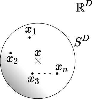
From the view point of vacuum condensation of topological defects which is expected to be a mechanism of confinement, it is reasonable to introduce multiple pairs of defects as the topological configuration to realize the true confining vacuum:

$$\partial_{\mu}\omega^{j}(x)=\sum_{s=1}^{n}Q_{s}\frac{\eta_{\mu\lambda}^{j}(x-x_{s})^{\lambda}}{|x-x_{s}|^{2}}g((x-x_{s})^{2})\ (j=3,\ \mu,\lambda=1,2,\cdots,D),$$ (33)

which is composed of $n$ topological defects with the respective topological charge $Q_{s}$ being located at $x_{s}\ (s=1,\cdots,n)$. When $n=1$, we put a defect at the origin $x_{s}=0$. This configuration also satisfies the condition for a residual gauge symmetry:

$$\partial^{\mu}\partial_{\mu}\omega^{j}(x)$$

$$= \sum_{s=1}^{n}Q_{s}\eta_{\mu\lambda}^{j}\partial^{\mu}\frac{(x-x_{s})^{\lambda}}{|x-x_{s}|^{2}}g((x-x_{s})^{2})$$

$$= \sum_{s=1}^{n}Q_{s}\eta_{\mu\lambda}^{j}\left[\frac{g^{\mu\lambda}}{|x-x_{s}|^{2}}g((x-x_{s})^{2})+2(x-x_{s})^{\mu}(x-x_{s})^{\lambda}\frac{\partial}{\partial(x-x_{s})^{2}}\left(\frac{g((x-x_{s})^{2})}{|x-x_{s}|^{2}}\right)\right]$$

$$= 0,$$ (34)

where we have used the antisymmetry $\eta_{\mu\lambda}^{j}=-\eta_{\lambda\mu}^{j}$. The above operation also can be understood as compactification of the spacetime $\mathbb{R}^{D}$ to a sphere $S^{D}$ with a large radius: $\mathbb{R}^{D}\rightarrow\ S^{D}$. Such compactification is usually adopted in the mathematical treatment of topological configurations in field theories. See figure 3.

In this description with multiple defects, we can prepare to discuss the condensation of magnetic monopoles. Indeed, this description is consistent with the dual superconductor picture of quark confinement where condensation of magnetic monopoles and antimonopoles occurs.

5 Conclusion and discussion

In the MA gauge, we have performed a detailed calculation for restoring the residual gauge symmetry in one diagonal gluon sector. The topological configurations considered in the previous paperKondo-Fukushima restore the residual gauge symmetry, but give divergences regardless of spacetime dimensions. These divergences come from IR and UV regions in the integral of the criterion $I_{\nu}$. The UV divergence in $I_{\nu}$ is associated with an infinite Euclidean action coming from the short distance singularity of the defect. This UV divergence can be avoided by choosing the topological defects with less singularity at its location for obtaining a finite Euclidean action to give non-trivial contribution to the path integral. It should be remarked that the topological defects acquire the same size from the above operations. The IR divergence in $I_{\nu}$ is avoided by introducing multiple topological defects with associated antidefects located at infinity. These operations make the Euclidean action finite and make the topological configurations valid for the path integral.

Moreover, if we introduce a topological configuration with multiple defects, these results are consistent with the confinement picture where the vacuum condensation of topological defects lead to confinement. Indeed, for $D=3$, they are consistent with the picture for quark confinement demonstrated by Polyakovmonople-plasma , where the gauge field becomes massive as a result of the Debye screening caused by magnetic monopole plasma, since multiple magnetic monopoles configurations are identified with the residual gauge symmetry for $D=3$ . A similar proposal for $D=4$ was suggested by Callan, Dashen, and Gross making use of meronsCallan-Dashen-Gross which should be examined in a future study. A physical picture of symmetry restoration due to topological configurations contributing to the path integral is provided. Therefore, based on this picture, it is necessary to discuss the condensation of topological defects in arbitrary dimensions.

To give the complete discussion for confinement, it is necessary to consider interactions among various fields, including different kinds of fields such as the ghost and gauge field. Therefore, we hope to investigate the restoration conditions of residual local gauge symmetry in sectors of all the fields in a subsequent paper.

Appendix A The criterion for the restoration of residual local gauge symmetry in a sector of the diagonal gluon

In the previous paper Kondo-Fukushima , we calculated (20) to obtain the criterion (21) using the Schwinger-Dyson equation of the anti-ghost field $\int d\mu\frac{\delta}{\delta c^{j}(y)}(e^{iS}F)$. However, this method is only applicable when considering the one gluon sector, as we used the relation $\frac{\delta e^{iS}}{\delta(-\bar{c}^{k}(y))}=\partial^{\mu}\delta_{\text{B}}a_{\mu}^{k}(y)$.

In what follows, we give a more general derivation of the criterion which is applicable to arbitrary sectors. we use the Schwinger-Dyson equations of the ghost field $\int d\mu\frac{\delta}{\delta c^{\ell}(x)}(e^{iS}F)$ and the NL field $\int d\mu\frac{\delta}{\delta B^{a}(x)}(e^{iS}F)$ to perform the calculation. This method does not require the use of the relation $\frac{\delta e^{iS}}{\delta(-\bar{c}^{k}(y))}=\partial^{\mu}\delta_{\text{B}}a_{\mu}^{k}(y)$, and hence it is applicable to any other sectors.

If the color symmetry is unbroken, the criterion (20) for the restoration of the residual local gauge symmetry in a sector of the diagonal gluon $a_{\nu}^{j}$ is reduced to

$$i\int d^{D}x\ e^{ip(x-y)}\partial^{x}_{\mu}\braket{\mathscr{J}_{\omega}^{\mu}(x)a_{\nu}^{j}(y)}$$

$$= \int d^{D}x\ e^{ip(x-y)}[\delta^{D}(x-y)\braket{\delta^{\omega}a_{\nu}^{j}(y)}+i\braket{\partial_{\mu}\mathscr{J}_{\omega}^{\mu}(x)a_{\nu}^{j}(y)}]$$

$$= \int d^{D}x\ e^{ip(x-y)}[\partial_{\nu}\omega^{j}(x)\delta^{D}(x-y)-\partial^{\mu}\omega^{\ell}(x)\braket{\partial_{\mu}\bar{c}^{\ell}(x)\delta_{\text{B}}a_{\nu}^{j}(y)}],$$ (35)

where we have used (19), $\partial_{\mu}\mathscr{J}_{\omega}^{\mu}=i\delta_{\text{B}}\partial_{\mu}\bar{c}^{j}\partial^{\mu}\omega^{j}+i\delta_{\text{B}}\partial^{\mu}(\mathscr{D}_{\mu}[\mathscr{A}]\bar{\mathscr{C}})^{a}\omega^{a}+i\delta_{\text{B}}(\mathscr{D}_{\mu}[\mathscr{A}]\bar{\mathscr{C}})^{a}\partial^{\mu}\omega^{a}$, $\braket{\delta_{B}(\cdots)}=0$ due to the physical state condition, and $\braket{0}{a^{j}_{\nu}(x)}{0}=0$ which follows from the Lorentz invariance of the vacuum $\ket{0}$. Because $\braket{\partial_{\mu}\bar{c}^{\ell}(x)\delta_{\text{B}}a_{\nu}^{j}(y)}$ has only longitudinal part, we can write

$$g_{\mu\lambda}\braket{\partial^{\lambda}\bar{c}^{\ell}(x)\delta_{\text{B}}a_{\nu}^{j}(y)}= \frac{\partial^{x}_{\mu}}{\partial_{x}^{2}}\braket{\partial_{\lambda}\partial^{\lambda}\bar{c}^{\ell}(x)\delta_{\text{B}}a_{\nu}^{j}(y)}.$$ (36)

The equation of motion for the NL field $B^{a}(x)$ is given by

$$0=\frac{\delta S}{\delta B^{a}(x)} =(\mathscr{D}_{\mu}[a]A^{\mu})^{a}(x)+\alpha B^{a}(x),$$ (37)

and the equation of motion for the $\ell$ component of $\bar{\mathscr{C}}$ is given by

$$0=\frac{\delta S}{\delta c^{\ell}(x)} =-i\partial_{\mu}\partial^{\mu}\bar{\mathscr{C}}^{\ell}(x)-igf^{\ell ab}A_{\mu}^{a}\partial^{\mu}\bar{C}^{b}(x)+igf^{\ell ab}\partial_{\mu}(A^{\mu a}\bar{C}^{b})(x)-ig^{2}f^{\ell cb}f^{bja}A^{\mu c}a_{\mu}^{j}\bar{C}^{a}(x)$$

$$=-i\partial_{\mu}\partial^{\mu}\bar{\mathscr{C}}^{\ell}(x)+ig(\partial^{\mu}A_{\mu}\times\bar{C})^{\ell}(x)+ig^{2}((a_{\mu}\times A^{\mu c})\times\bar{C})^{\ell}(x)$$

$$=-i\partial_{\mu}\partial^{\mu}\bar{\mathscr{C}}^{\ell}(x)+ig(\mathscr{D}_{\mu}[a]A^{\mu}\times\bar{C})^{\ell}(x)$$ (38)

where we have used $f^{\ell cb}f^{bja}A^{\mu c}a_{\mu}^{j}\bar{C}^{a}=(A^{\mu}\times(a_{\mu}\times\bar{C}))^{\ell}=-(a_{\mu}\times(\bar{C}\times A^{\mu}))-(\bar{C}\times(A^{\mu}\times a_{\mu}))=-((a_{\mu}\times A^{\mu})\times\bar{C})^{\ell}$. If we use (37), (38) reads

$$0=\frac{\delta S}{\delta c^{\ell}(x)}=-i\partial_{\mu}\partial^{\mu}\bar{c}^{\ell}(x)+ig\left(\left(\frac{\delta S}{\delta B(x)}-\alpha B\right)\times\bar{C}\right)^{\ell}(x).$$ (39)

Therefore, using the Schwinger-Dyson equation $\int d\mu\frac{\delta}{\delta\Phi(x)}(e^{iS}F)=0$, (36) is reduced to

$$\frac{\partial^{x}_{\mu}}{\partial_{x}^{2}}\braket{\partial^{x}_{\lambda}\partial^{\lambda}\bar{c}^{\ell}(x)\delta_{\text{B}}a_{\nu}^{j}(y)}= \frac{\partial^{x}_{\mu}}{\partial_{x}^{2}}\Braket{\left\{i\frac{\delta S}{\delta c^{\ell}(x)}+g\left(\left(\frac{\delta S}{\delta B(x)}-\alpha B\right)\times\bar{C}\right)^{\ell}(x)\right\}\delta_{\text{B}}a_{\nu}^{j}(y)}$$

$$= -\frac{\partial^{x}_{\mu}}{\partial_{x}^{2}}\Braket{\frac{\delta}{\delta c^{\ell}(x)}(\mathscr{D}_{\nu}\mathscr{C})^{j}(y)}=\delta^{\ell j}\frac{\partial^{x}_{\mu}\partial^{x}_{\nu}}{\partial_{x}^{2}}\delta^{D}(x-y),$$ (40)

where we have used $\braket{\cdots}=\int d\mu\ e^{iS}(\cdots)$, $\braket{(B\times\bar{C})^{\ell}(x)\delta_{\text{B}}a_{\nu}^{j}(y)}=\braket{\delta_{\text{B}}(B\times\bar{C})^{\ell}(x)a_{\nu}^{j}(y)}=0$ and $\braket{0}{A_{\nu}^{a}(x)}{0}=0$ which follows from the Lorentz invariance. Consequently, the criterion for the restoration of the residual local gauge symmetry in a sector of the diagonal gluon $a_{\nu}^{j}$ is given by

$$0=\lim_{p\rightarrow\ 0}\int d^{D}x\ e^{ip(x-y)}\partial^{\mu}\omega^{j}(x)\left(g_{\mu\nu}-\frac{\partial^{x}_{\mu}\partial^{x}_{\nu}}{\partial_{x}^{2}}\right)\delta^{D}(x-y).$$ (41)

Appendix B The behavior of $h(x^{2})$h_D=3

In $D=3$, we consider $SU(2)$ gauge–scalar model with a radially fixed scalar field in the adjoint representation $\phi^{A}(x)=v\hat{\phi}^{A}(x)$ described by the Lagrangian density

$$\mathscr{L}(x) =-\frac{1}{4}\mathscr{F}_{\mu\nu}^{A}(x)\mathscr{F}^{\mu\nu A}(x)+\frac{1}{2}(\mathscr{D}_{\mu}[A]\phi)^{A}(x)(\mathscr{D}^{\mu}[A]\phi)^{A}(x)+\lambda(\phi^{A}\phi^{A}-v^{2}).$$ (42)

We adopt the Anzatz:

$$\hat{\phi}^{A}(x) =\frac{x^{A}}{r},$$

$$gA_{\mu}^{A}(x) =-\epsilon_{A\mu\lambda}\frac{x^{\lambda}}{x^{2}}h(r^{2}).$$ (43)

Since $Q\propto g^{-1}$, this Anzatz corresponds to the topological configuration (22).

Using the Anzatz (43), the Euclidean action for this model (42) is given by

$$S =\int d^{3}x\left\{-\frac{1}{4}\mathscr{F}_{\mu\nu}(x)\cdot\mathscr{F}_{\mu\nu}(x)+\frac{1}{2}\mathscr{D}_{\mu}[A]\phi(x)\cdot\mathscr{D}_{\mu}[A]\phi(x)-V(\phi(x))\right\}$$

$$=\frac{4\pi}{g^{2}}\int_{0}^{\infty}dr\ \left[\left(\frac{dh(r^{2})}{dr}\right)^{2}+\frac{h^{2}(r^{2})(h(r^{2})-2)^{2}}{2r^{2}}+g^{2}v^{2}(h(r^{2})-1)^{2}\right].$$ (44)

If $h(r^{2})\equiv 1$, this action diverges as $r\rightarrow 0$ due to the 2nd term in the integrand. In order for this integration to converge to give a finite Euclidean action, we find that the boundary condition must be imposed:

$$h(r^{2})\rightarrow\ \begin{cases}1+\mathcal{O}(1/r)&(r\rightarrow\ \infty)\\ \mathcal{O}\left((r^{2})^{\delta}\right)&(\delta>1/4,\ r\rightarrow\ 0)\end{cases}.$$ (45)

Therefore, $h(r^{2})$ approaches 1 rapidly in the long distance $r\gg 1$, while $h(r^{2})$ approaches zero ($h(r^{2})\rightarrow\ 0$) in the short distance $r\ll 1$.

Under the Anzatz (43), the field equations of the model (42) are obtained as

$$\frac{d^{2}h(r^{2})}{dr^{2}} =\frac{h(r^{2})(h(r^{2})-1)(h(r^{2})-2)}{r^{2}}+g^{2}v^{2}(h-1),$$

$$0 =(h(r^{2})-1)^{2}-\lambda r^{2}.$$ (46)

The 2nd equation determines $\lambda=\lambda(r)$. In order to obtain the asymptotic behavior of $h(r)$ for $r\ll 1$, we use $|h(r^{2})|\ll 1$ and linearize the 1st equation:

$$\rho^{2}\frac{d^{2}h(\rho)}{d\rho^{2}}-2h(\rho)-\rho^{2}h(\rho)=-\rho^{2}\ (\rho:=gvr).$$ (47)

This equation for $h(\rho)$ has a general solution:

$$h(\rho)= C_{1}\left(\cosh\rho-\frac{\sinh\rho}{\rho}\right)+C_{2}\left(\frac{\cosh\rho}{\rho}-\sinh\rho\right)$$

$$+1-\left(\cosh\rho-\frac{\sinh\rho}{\rho}\right)\text{Chi}\ \rho-\left(\frac{\cosh\rho}{\rho}-\sinh\rho\right)\text{Shi}\ \rho$$ (48)

where we have defined the hyperbolic cosine and sine integrals, denoted as $\text{Chi}\ \rho$ and $\text{Shi}\ \rho$ respectively, with the Euler constant $\gamma$:

$$\text{Chi}\ \rho:=\gamma+\ln\rho+\int_{0}^{\rho}dt\frac{\cosh\rho-1}{t},\ \text{Shi}\ \rho:=\int_{0}^{\rho}dt\frac{\sinh\rho}{t}.$$ (49)

Using the boundary conditions $h(0)=0$ and $\frac{dh(0)}{dr}=0$, we obtain $C_{2}=0$ and hence

$$h(\rho)=C_{1}\left(\cosh\rho-\frac{\sinh\rho}{\rho}\right)+1-\left(\cosh\rho-\frac{\sinh\rho}{\rho}\right)\text{Chi}\ \rho-\left(\frac{\cosh\rho}{\rho}-\sinh\rho\right)\text{Shi}\ \rho,$$ (50)

which has the expansion:

$$h(r)=\tilde{C}(gvr)^{2}-\frac{1}{3}(gvr)^{2}\ln(gvr)+\mathcal{O}(r^{4})\ (r\ll 1),$$ (51)

where we have defined $\tilde{C}:=\frac{1}{9}(4-3\gamma+3C_{1})$. Therefore, $h(x^{2})$ approaches zero of order $r^{2\delta}=(x^{2})^{\delta}(\delta\cong 1)$ in the short distance $r\ll 1$.

Appendix C The details of calculation for the criterion for residual local gauge symmetry restoration with $\widetilde{\partial^{\mu}\omega_{\delta}}^{j}(q)$

We calculate (32):

$$I_{\nu}=\lim_{p\rightarrow\ 0}iQC_{D}\eta^{\mu\lambda j}\int\frac{d^{D}k}{(2\pi)^{D}}\frac{q_{\lambda}}{|q|^{D+2\delta}}\left(g_{\mu\nu}-\frac{k_{\mu}k_{\nu}}{k^{2}}\right)\ (q=p-k).$$ (52)

By using the Feynman parameter integral:

$$\frac{1}{a^{n}b}=n\int_{0}^{1}d\alpha\frac{\alpha^{n-1}}{(\alpha a+(1-\alpha)b)^{n+1}},$$ (53)

we can express the integral as

$$I_{\nu} =-iQC_{D}\left(\frac{D}{2}+\delta\right)\lim_{p\rightarrow\ 0}\eta^{\mu\lambda j}p_{\lambda}\int_{0}^{1}d\alpha\int\frac{d^{D}k}{(2\pi)^{D}}k_{\mu}k_{\nu}\frac{\alpha^{\frac{D}{2}+\delta-1}}{\{(k-\alpha p)^{2}+\alpha(1-\alpha)p^{2}\}^{\frac{D}{2}+\delta+1}}$$

$$=-iQC_{D}\left(\frac{D}{2}+\delta\right)\lim_{p\rightarrow\ 0}\eta^{\mu\lambda j}p_{\lambda}\int_{0}^{1}d\alpha\int\frac{d^{D}\ell}{(2\pi)^{D}}(\ell+\alpha p)_{\mu}(\ell+\alpha p)_{\nu}\frac{\alpha^{\frac{D}{2}+\delta-1}}{\{\ell^{2}+\alpha(1-\alpha)p^{2}\}^{\frac{D}{2}+\delta+1}}$$

$$=-iQC_{D}\left(\frac{D}{2}+\delta\right)\lim_{p\rightarrow\ 0}\eta^{\mu\lambda j}p_{\lambda}\int_{0}^{1}d\alpha\int\frac{d^{D}\ell}{(2\pi)^{D}}\ell_{\mu}(\ell+\alpha p)_{\nu}\frac{\alpha^{\frac{D}{2}+\delta-1}}{\{\ell^{2}+\alpha(1-\alpha)p^{2}\}^{\frac{D}{2}+\delta+1}},$$ (54)

where we have defined $\ell_{\mu}:=k_{\mu}-\alpha p_{\mu}$ and used the antisymmetry $\eta^{\mu\lambda j}=-\eta^{\lambda\mu j}$ repeatedly. Using the fact that the integral of an odd function over the interval $(-\infty,\infty)$ vanishes, we can make the replacement: $\ell_{\mu}(\ell+\alpha p)_{\nu}\rightarrow\ \ell_{\mu}\ell_{\nu}\rightarrow\ \frac{1}{D}\ell^{2}g_{\mu\nu}$ to obtain:

$$I_{\nu} =-i\frac{QC_{D}}{D}\left(\frac{D}{2}+\delta\right)\lim_{p\rightarrow\ 0}\eta_{\nu\lambda}^{j}p^{\lambda}\int_{0}^{1}d\alpha\int\frac{d^{D}\ell}{(2\pi)^{D}}\frac{\alpha^{\frac{D}{2}+\delta-1}\ell^{2}}{\{\ell^{2}+\alpha(1-\alpha)p^{2}\}^{\frac{D}{2}+\delta+1}}$$ (55)

If we estimate the contribution of the UV region $k>k_{R}\gg 1$ to $I_{\nu}$, we can take the limit $p\rightarrow\ 0$ of the integrand, which is equivalent to the replacement $\ell_{\mu}=k_{\mu}$:

$$I_{\nu}\rightarrow\ -i\frac{QC_{D}}{D}\left(\frac{D}{2}+\delta\right)\lim_{p\rightarrow\ 0}\eta_{\nu\lambda}^{j}p^{\lambda}\int_{0}^{1}d\alpha\int d\Omega_{D}\int_{k_{R}}^{\infty}\frac{dk\ k^{D-1}}{(2\pi)^{D}}\frac{\alpha^{\frac{D}{2}+\delta-1}}{k^{D+2\delta}}$$

$$= -i\frac{QC_{D}}{(4\pi)^{\frac{D}{2}}\Gamma\left(\frac{D}{2}+1\right)}\left(\frac{D}{2}+\delta\right)\lim_{p\rightarrow\ 0}\eta_{\nu\lambda}^{j}p^{\lambda}\int_{0}^{1}d\alpha\int_{k_{R}}^{\infty}dk\frac{\alpha^{\frac{D}{2}+\delta-1}}{k^{2\delta+1}}$$

$$= -i\frac{QC_{D}}{(4\pi)^{\frac{D}{2}}\Gamma\left(\frac{D}{2}+1\right)}\lim_{p\rightarrow\ 0}\eta_{\nu\lambda}^{j}p^{\lambda}[\alpha^{\frac{D}{2}+\delta}]_{0}^{1}\left[-\frac{1}{2\delta}\frac{1}{k^{2\delta}}\right]_{k_{R}}^{\infty}$$

$$= -i\frac{QC_{D}}{2\delta(4\pi)^{\frac{D}{2}}\Gamma\left(\frac{D}{2}+1\right)}\lim_{p\rightarrow\ 0}\eta_{\nu\lambda}^{j}p^{\lambda}\frac{1}{k_{R}^{2\delta}}=0\ \left(\delta>1/4\right),$$ (56)

where $\Omega_{D}$ denotes the volume of the sphere $S^{D-1}$ with a unit radius. Consequently, the UV region of $k$ does not contribute to $I_{\nu}$ in the limit $p\rightarrow\ 0$ and we can ignore the UV region of $k$ in examining the restoration of the residual local gauge symmetry.

References

• [1] Y. Nambu, Phys. Rev. D10, 4262(1974).
G. ’t Hooft, in: High Energy Physics, edited by A. Zichichi (Editorice Compositori, Bologna, 1975).
S. Mandelstam, Phys. Report 23, 245(1976).
M.N. Chernodub, M.I. Polikarpov, Abelian projections and monopoles, Lectures given at NATO Advanced Study Institute on Confinement, Duality and Nonperturbative Aspects of QCD, Cambridge, England, 23 Jun - 4 Jul 1997, [arXiv:hep-th/9710205]
K.-I. Kondo, S. Kato, A. Shibata and T. Shinohara, Phys. Rept. 579, 1(2015) [arXiv:1409.1599 [hep-th]].
• [2] T. Kugo and I. Ojima, Suppl. Prog. Theor. Phys. 66, 1-130 (1979).
T. Kugo and I. Ojima, Phys. Lett. 73B, 459 (1978); Prog. Theor. Phys. 60, 1869 (1978); 61, 294, 644 (1979).
• [3] T. Kugo, Quantum theory of gauge fields, I, II, in Japanese (Baifu-kan, Tokyo, 1989).
T. Kugo, arXiv: hep-th/9511033
• [4] H. Hata, Prog. Theor. Phys. 67, 1607 (1982)
• [5] K.-I. Kondo and N. Fukushima, PTEP 2022, no.5, 053B05 (2022).
• [6] H. Nakajima and S. Furui, Phys. Rev. D 69, 074505 (2004). arXiv: hep-lat/0305010
H. Nakajima and S. Furui, Few-Body Systems 40, 101–128 (2006). arXiv: hep-lat/0503029
H. Nakajima and S. Furui, Phys. Rev. D 73, 094506 (2006). arXiv: hep-lat/0602027
H. Nakajima and S. Furui, Braz. J. Phys. 37, 186–192, (2007). arXiv: hep-lat/0609024.
• [7] A. Sternbeck, Ph.D. Thesis, arXiv: hep-lat/0609016.
A. Sternbeck et al, PoS LAT2006, 076 (2006). arXiv: hep-lat/0610053.
• [8] P. Boucaud, Th. Bruntjen, J.P. Leroy, A. Le Yaouanc, A.Y. Lokhov, J. Micheli, O. Pene and J. Rodriguez-Quintero, JHEP 0606, 001 (2006). arXiv: hep-ph/0604056
• [9] I.L. Bogolubsky, E.M. Ilgenfritz, M. Muller-Preussker and A. Sternbeck, Phys. Lett. B676, 69-73 (2009). arXiv: 0901.0736[hep-lat]
• [10] A. Cucchieri and T. Mendes, PoS LAT2007, 297 (2007). arXiv: 0710.0412 [hep-lat].
A. Cucchieri and T. Mendes, Phys. Rev. D78, 094503 (2008). arXiv: 0804.2371[hep-lat].
• [11] A. Sternbeck, L. von Smekal, D.B. Leinweber and A.G. Williams, PoS LAT2007, 340(2007). arXiv: 0710.1982[hep-lat]
• [12] A. Kronfeld, M. Laursen, G. Schierholz and U.-J. Wiese, Phys. Lett. B198, 516(1987).
K.-I. Kondo, Phys. Rev. D 58, 105019 (1998). arXiv: [hep-th/9801024]
K.-I. Kondo, Phys. Lett. B514, 335-345 (2001). [hep-th/0105299]
K.-I. Kondo, Phys. Lett. B572, 210(2003). arXiv: [hep-th/0306195]
• [13] E. Corrigan and D.B. Fairlie, Phys. Lett. B 67, 69 (1977).
G. ’t Hooft, Phys.Rev. D14, 3432-3450 (1976); Erratum-ibid. D18, 2199 (1978).
F. Wilczek, in “Quark Confinement and Field Theory” eds. by D. Stump and D. Weingarten, (Wiley, New York, 1977).
• [14] A. Actor, Rev. Mod. Phys. 51, 461(1979).
• [15] H. B. Nielsen and P. Olesen, Nucl. Phys. B160, 380(1979).
• [16] Tai Tsun Wu, Chen Ning Yang, Phys. Rev. D12, 3845(1975). T.T. Wu and C.N. Yang, Nucl. Phys. B107, 365-380 (1976). T.T. Wu and C.N. Yang, Phys. Rev. D14, 437(1976).
• [17] G. ’t Hooft, Nucl. Phys. B79, 276(1974). A. M. Polyakov, JETP Lett. 20, 194(1974).
• [18] V. De Alfaro, S. Fubini and G. Furlan, Phys. Lett. B65, 163(1976).
C.G. Callan, R. Dashen and D.J. Gross, Phys. Rev. D17, 2717(1978).
• [19] A.A. Belavin, A.M. Polyakov, A.S. Shwarts and Yu.S. Tyupkin, Phys. Lett. B59, 85(1975).
• [20] A.M. Polyakov, Nucl. Phys. B120, 429(1977).
• [21] C.G. Callan, R. Dashen and D.J. Gross, Phys. Rev. D17, 2717(1978).
• [22] S. Nishino, R. Matsudo, M. Warschinke, and K.-I. Kondo, PTEP2018, 103B04 (2018).