1 Introduction

After the July 4th 2012 announcement [1, 2] of the discovery of a resonance compatible with the Standard Model (SM) Higgs boson, no other particle has been detected. On the other hand, experimental data from the last decade is being used to increase the precision of our knowledge on many different observables, resulting in very accurate indirect searches.

In the absence of a specific New Physics (NP), one approach to studying possible deviations from the SM predictions is the Standard Model Effective Field Theory (SMEFT) [3, 4] that is a basis of independent operators, ordered in terms of mass dimensions, invariant under the SM gauge symmetry and constructed out of the SM fields 111As the nature of the Higgs field is still uncertain up to a certain degree, alternative effective descriptions have been proposed [5, 6, 7, 8, 9, 10, 11, 12, 13, 14], providing different expectations in certain observables.. The hope is to extract information on the ultraviolet (UV) completion by identifying specific patterns and synergies among the SMEFT operators.

Even restricting to the subgroup with mass dimension d=6๐‘‘6d=6, the number of such operators is tremendous, 2499, considering all the flavour contractions [15]. Although it is possible to perform global fits on a reduced subset of operators under certain reasonable assumptions, no clear evidence of a specific NP has emerged (see for example Ref. [16] for a recent fit to the electroweak Higgs data). This occurs despite the rapport on some apparent anomalies in particle physics. To be mentioned is the new measurement from the CDF II collaboration of the W๐‘ŠW-gauge boson mass [17], that exceeds the SM prediction by approximately 7โ€‹ฯƒ7๐œŽ7\sigma (but not confirmed by the last ATLAS result [18]): assuming that the CDF II result is correct, different explanations have been proposed to account for the deviation from the SM prediction, from tree-level modification of the muon decay induced by exotic leptons (see for example Refs. [19, 20, 21]), to loop quantum corrections to the two-point functions of the SM gauge bosons (see for example Refs. [22, 23]). Another example is the charged B๐ตB-anomalies, hinting to lepton flavour universality violation in the B๐ตB-meson semi-leptonic decays Bโ†’D(โˆ—)โ€‹lโ€‹ฮฝโ†’๐ตsuperscript๐ทโˆ—๐‘™๐œˆB\rightarrow D^{(\ast)}l\nu: the experimental results, combining data from the BaBar [24, 25] and Belle [26, 27, 28] collaborations, exceeds the SM prediction by 3.5โ€‹ฯƒ3.5๐œŽ3.5\sigma [29]. Recently, the LHCb collaboration [30] announced its results on this observable, lowering the deviation of the world average to the 3โ€‹ฯƒ3๐œŽ3\sigma level. Considering that other apparent discrepancies in the B๐ตB-decays have been clarified by the LHCb collaboration [31, 32], explanations of the charged B๐ตB-anomalies in terms of exotic charged gauge bosons (see e.g. Ref. [33]) or a charged Higgs boson (see e.g. Refs. [34, 35, 36]) or leptoquarks (see e.g. Refs. [37, 38, 39]) appear much less plausible, even if still possible.

This bottom-up approach has been largely adopted in the recent literature and, given the lack of clear indications towards a specific NP, we will abandon it here. Instead, we will assume a concrete extension of the SM and analyse its effects in the low-energy effective Lagrangian approximation, with the aim of exploring the associated phenomenology in the reduced NP parameter space. Our choice is the two Higgs doublet models (2HDMs) [40, 41, 42, 43, 44, 45, 46, 47]. Although such extensions of the SM do not address the most pressing questions like the origin of the active neutrino masses, the existence of dark matter and the baryon asymmetry of the Universe, they are nevertheless a useful theoretical laboratory. They permit to investigate the room left by the present flavour and Higgs sector experimental data for NP in the scalar potential and in the effective Yukawa couplings. They are also interesting in the context of supersymmetric extensions of the SM.

Most of the analyses present in the literature in the framework of the EFT approach treat data on the electroweak (EW) and Higgs sectors separately from flavour data. Only a few examples appeared attempting to merge all the information, although at the cost of assuming specific flavour structures. This is the case of Refs. [48, 49, 50] and subsequent Refs. [51, 52], where the generic conclusion is that flavour data and EW/Higgs data are close to being comparable to each other in their sensitivity to NP effects. In this paper, we will extend upon the study in Refs. [49, 50] based on the Minimal Flavour Violation (MFV) ansatz [53, 54, 55, 56, 57, 58] and on the Froggatt-Nielsen (FN) mechanism [59], two very well-known contexts in the literature, see Refs. [60, 61, 62, 63, 64, 65, 66, 67, 68, 69, 70, 71, 72, 73, 74, 75, 76, 77] and [78, 79, 80, 81, 82], respectively. The MFV and the FN represent two extreme cases: the fermion-Higgs couplings are flavour conserving or largely violating it, respectively; moreover, there is only one universal CP violating phase for each fermion sector in the MFV case, while several phases are present in the FN one. Our framework is the effective Lagrangian derived from Z2subscript๐‘2Z_{2}-symmetric versions of the 2HDMs, where the role of the Z2subscript๐‘2Z_{2} symmetry is to ensure protection from tree-level flavour changing neutral current (FCNC) contributions [41], but still allowing effects in flavour changing processes due to the presence of charged Higgses. Thus, they represent a middle ground between the two aforementioned constructions based on flavour symmetries. Furthermore, as we will discuss, in the effective Yukawa couplings there is only one universal CP violating phase for all fermions of the SM.

Our analysis is valid near the decoupling limit, which will be defined in Sect. 2, of all the heavy scalar states. This hypothesis is motivated by the absence of any discovery of additional scalars and we will assume them to be heavy enough to justify an effective description. In consequence, all the heavy scalars are almost degenerate in mass, so their low-energy effects are to a good approximation controlled by only one mass scale. This last condition will be relaxed when discussing the possible explanation of the CDF II measurement of the W๐‘ŠW mass.

The bulk of our analysis depends on only three new NP parameters, that is the common mass of the heavier scalar degrees of freedom, one coupling in the scalar potential and tanโกฮฒ๐›ฝ\tan\beta, characteristic of the 2HDM constructions. The predictive power is therefore high and we make use of it providing the expected maximum deviation in the triple Higgs coupling from its SM value for each Z2subscript๐‘2Z_{2}-symmetric 2HDM realisation.

The structure of the paper can be read in the table of Contents.

2 The 2HDM Lagrangian

The general 2HDM and its Z2subscript๐‘2Z_{2} symmetric versions have been extensively discussed in the literature (see for example Refs. [83, 84, 85, 86, 87, 88, 89, 90, 91]). The main motivation for imposing a Z2subscript๐‘2Z_{2} symmetry on a 2HDM is to forbid tree-level FCNC contributions. For the sake of easy reference to the Z2subscript๐‘2Z_{2} symmetric versions and for fixing the notation used throughout the paper, we collect here (and in the App. A) their key ingredients.

A discrete Abelian Z2subscript๐‘2Z_{2} symmetry quantum numbers are assigned to the two Higgs doublets ฮฆ1subscriptฮฆ1\Phi_{1} and ฮฆ2subscriptฮฆ2\Phi_{2}, even and odd under Z2subscript๐‘2Z_{2} respectively, and to the fermion fields. The assignment of the Z2subscript๐‘2Z_{2} quantum numbers identifies the original basis for those fields. Focusing first on the scalar potential of the model, the Z2subscript๐‘2Z_{2} symmetry restricts its form (see App. A), and the vacuum of the model is fixed in terms of the mass parameters and the couplings to be:

โŸจฮฆ1โ€ โ€‹ฮฆ1โŸฉ=v122,โŸจฮฆ2โ€ โ€‹ฮฆ2โŸฉ=v222,โŸจฮฆ1โ€ โ€‹ฮฆ2โŸฉ=v1222,v12+v22=v2formulae-sequencedelimited-โŸจโŸฉsuperscriptsubscriptฮฆ1โ€ subscriptฮฆ1superscriptsubscript๐‘ฃ122formulae-sequencedelimited-โŸจโŸฉsuperscriptsubscriptฮฆ2โ€ subscriptฮฆ2superscriptsubscript๐‘ฃ222formulae-sequencedelimited-โŸจโŸฉsuperscriptsubscriptฮฆ1โ€ subscriptฮฆ2superscriptsubscript๐‘ฃ1222superscriptsubscript๐‘ฃ12superscriptsubscript๐‘ฃ22superscript๐‘ฃ2\langle\Phi_{1}^{\dagger}\Phi_{1}\rangle=\dfrac{v_{1}^{2}}{2}\,,\qquad\langle\Phi_{2}^{\dagger}\Phi_{2}\rangle=\dfrac{v_{2}^{2}}{2}\,,\qquad\langle\Phi_{1}^{\dagger}\Phi_{2}\rangle=\dfrac{v_{12}^{2}}{2}\,,\qquad v_{1}^{2}+v_{2}^{2}=v^{2}\, (2.1)

where v1subscript๐‘ฃ1v_{1} and v2subscript๐‘ฃ2v_{2} are real, v12subscript๐‘ฃ12v_{12} is in general complex, and v=246โ€‹GeV๐‘ฃ246GeVv=246\ \text{GeV}. Moreover, the CP violating phase of the mixed Higgs condensate we denote as

ฮพโ‰กargโก(ฮฆ1โ€ โ€‹ฮฆ2).๐œ‰superscriptsubscriptฮฆ1โ€ subscriptฮฆ2\xi\equiv\arg\left(\Phi_{1}^{\dagger}\Phi_{2}\right)\,. (2.2)

It is convenient to rewrite the scalar potential in the Higgs basis where only one of the two Higgses acquires a VEV. Performing Uโ€‹(2)๐‘ˆ2U(2) rotations of the Higgs fields in a two-dimensional complex plane by the angle ฮฒ๐›ฝ\beta defined as

tanโกฮฒ=v2v1,๐›ฝsubscript๐‘ฃ2subscript๐‘ฃ1\tan\beta=\frac{v_{2}}{v_{1}}\,, (2.3)

one obtains:

Vโ€‹(H1,H2)=๐‘‰subscript๐ป1subscript๐ป2absent\displaystyle V(H_{1},H_{2})=\, m~12โ€‹H1โ€ โ€‹H1+m~22โ€‹H2โ€ โ€‹H2โˆ’(m~122โ€‹H1โ€ โ€‹H2+h.c.)+12โ€‹ฮป~1โ€‹(H1โ€ โ€‹H1)2+superscriptsubscript~๐‘š12superscriptsubscript๐ป1โ€ subscript๐ป1superscriptsubscript~๐‘š22superscriptsubscript๐ป2โ€ subscript๐ป2superscriptsubscript~๐‘š122superscriptsubscript๐ป1โ€ subscript๐ป2h.c.limit-from12subscript~๐œ†1superscriptsuperscriptsubscript๐ป1โ€ subscript๐ป12\displaystyle\widetilde{m}_{1}^{2}H_{1}^{\dagger}H_{1}+\widetilde{m}_{2}^{2}H_{2}^{\dagger}H_{2}-\left(\widetilde{m}_{12}^{2}H_{1}^{\dagger}H_{2}+\text{h.c.}\right)+\dfrac{1}{2}\widetilde{\lambda}_{1}\left(H_{1}^{\dagger}H_{1}\right)^{2}+
+12โ€‹ฮป~2โ€‹(H2โ€ โ€‹H2)2+ฮป~3โ€‹(H1โ€ โ€‹H1)โ€‹(H2โ€ โ€‹H2)+ฮป~4โ€‹(H1โ€ โ€‹H2)โ€‹(H2โ€ โ€‹H1)+12subscript~๐œ†2superscriptsuperscriptsubscript๐ป2โ€ subscript๐ป22subscript~๐œ†3superscriptsubscript๐ป1โ€ subscript๐ป1superscriptsubscript๐ป2โ€ subscript๐ป2limit-fromsubscript~๐œ†4superscriptsubscript๐ป1โ€ subscript๐ป2superscriptsubscript๐ป2โ€ subscript๐ป1\displaystyle+\dfrac{1}{2}\widetilde{\lambda}_{2}\left(H_{2}^{\dagger}H_{2}\right)^{2}+\widetilde{\lambda}_{3}\left(H_{1}^{\dagger}H_{1}\right)\left(H_{2}^{\dagger}H_{2}\right)+\widetilde{\lambda}_{4}\left(H_{1}^{\dagger}H_{2}\right)\left(H_{2}^{\dagger}H_{1}\right)+ (2.4)
+[12โ€‹ฮป~5โ€‹(H1โ€ โ€‹H2)2+ฮป~6โ€‹(H1โ€ โ€‹H1)โ€‹(H1โ€ โ€‹H2)+ฮป~7โ€‹(H2โ€ โ€‹H2)โ€‹(H1โ€ โ€‹H2)+h.c.].delimited-[]12subscript~๐œ†5superscriptsuperscriptsubscript๐ป1โ€ subscript๐ป22subscript~๐œ†6superscriptsubscript๐ป1โ€ subscript๐ป1superscriptsubscript๐ป1โ€ subscript๐ป2subscript~๐œ†7superscriptsubscript๐ป2โ€ subscript๐ป2superscriptsubscript๐ป1โ€ subscript๐ป2h.c.\displaystyle+\left[\dfrac{1}{2}\widetilde{\lambda}_{5}\left(H_{1}^{\dagger}H_{2}\right)^{2}+\widetilde{\lambda}_{6}\left(H_{1}^{\dagger}H_{1}\right)\left(H_{1}^{\dagger}H_{2}\right)+\widetilde{\lambda}_{7}\left(H_{2}^{\dagger}H_{2}\right)\left(H_{1}^{\dagger}H_{2}\right)+\text{h.c.}\right]\,.

The expressions for the tilde parameters in terms of the parameters defined in the original basis are given in the App. A. The parameters m~12superscriptsubscript~๐‘š12\widetilde{m}_{1}^{2}, m~22superscriptsubscript~๐‘š22\widetilde{m}_{2}^{2}, ฮป~1subscript~๐œ†1\widetilde{\lambda}_{1}, ฮป~2subscript~๐œ†2\widetilde{\lambda}_{2}, ฮป~3subscript~๐œ†3\widetilde{\lambda}_{3} and ฮป~4subscript~๐œ†4\widetilde{\lambda}_{4} are real, while m~122superscriptsubscript~๐‘š122\widetilde{m}_{12}^{2}, ฮป~5subscript~๐œ†5\widetilde{\lambda}_{5}, ฮป~6subscript~๐œ†6\widetilde{\lambda}_{6} and ฮป~7subscript~๐œ†7\widetilde{\lambda}_{7} are in general complex. However, as discussed in App. A, for the Z2subscript๐‘2Z_{2} symmetric models there are only two independent CP-violating phases:

ฮธ1โ‰ก12โ€‹argโก(ฮป~62โ€‹ฮป~5โˆ—),ฮธ2โ‰ก12โ€‹argโก(ฮป~72โ€‹ฮป~5โˆ—).formulae-sequencesubscript๐œƒ112superscriptsubscript~๐œ†62superscriptsubscript~๐œ†5โˆ—subscript๐œƒ212superscriptsubscript~๐œ†72superscriptsubscript~๐œ†5โˆ—\theta_{1}\equiv\dfrac{1}{2}\arg{(\widetilde{\lambda}_{6}^{2}\widetilde{\lambda}_{5}^{\ast})}\,,\qquad\qquad\theta_{2}\equiv\dfrac{1}{2}\arg{(\widetilde{\lambda}_{7}^{2}\widetilde{\lambda}_{5}^{\ast})}\,. (2.5)

Enforcing the condition that

โŸจH1โ€ โ€‹H1โŸฉ=v22,โŸจH2โ€ โ€‹H2โŸฉ=0,formulae-sequencedelimited-โŸจโŸฉsubscriptsuperscript๐ปโ€ 1subscript๐ป1superscript๐‘ฃ22delimited-โŸจโŸฉsubscriptsuperscript๐ปโ€ 2subscript๐ป20\langle H^{\dagger}_{1}H_{1}\rangle=\dfrac{v^{2}}{2}\,,\qquad\qquad\langle H^{\dagger}_{2}H_{2}\rangle=0\,, (2.6)

leads to two relations between four of the parameters,

m~12=โˆ’12โ€‹ฮป~1โ€‹v2,m~122=โˆ’12โ€‹ฮป~6โ€‹v2,formulae-sequencesuperscriptsubscript~๐‘š1212subscript~๐œ†1superscript๐‘ฃ2superscriptsubscript~๐‘š12212subscript~๐œ†6superscript๐‘ฃ2\widetilde{m}_{1}^{2}=-\dfrac{1}{2}\widetilde{\lambda}_{1}v^{2}\,,\qquad\qquad\widetilde{m}_{12}^{2}=-\dfrac{1}{2}\widetilde{\lambda}_{6}v^{2}\,, (2.7)

reducing the number of independent parameters.

In the vacuum defined by the scalar potential, five degrees of freedom acquire masses, while the remaining three remain massless, corresponding to the three longitudinal components of the EW gauge bosons. The two charged Higgs bosons Hยฑsuperscript๐ปplus-or-minusH^{\pm} receive a mass that reads

mHยฑ2=m~22+12โ€‹ฮป~3โ€‹v2,superscriptsubscript๐‘šsubscript๐ปplus-or-minus2superscriptsubscript~๐‘š2212subscript~๐œ†3superscript๐‘ฃ2m_{H_{\pm}}^{2}=\widetilde{m}_{2}^{2}+\dfrac{1}{2}\widetilde{\lambda}_{3}v^{2}\,, (2.8)

while a mixing is present in the neutral sector and the corresponding mass eigenvalues can be identified with the SM Higgs boson hโ„Žh, a heavier CP-even Higgs H๐ปH, and a heavier CP-odd Higgs A๐ดA. At the second order in the expansion v2/m~22superscript๐‘ฃ2superscriptsubscript~๐‘š22v^{2}/\widetilde{m}_{2}^{2} their masses read

mh2superscriptsubscript๐‘šโ„Ž2\displaystyle m_{h}^{2} =v2โ€‹{ฮป~1โˆ’|ฮป~6|2โ€‹v2m~22โˆ’12โ€‹[(2โ€‹ฮป~1โˆ’ฮป~3โˆ’ฮป~4)โ€‹|ฮป~6|2โˆ’12โ€‹(ฮป~5โˆ—โ€‹ฮป~62+h.c.)]โ€‹(v2m~22)2},absentsuperscript๐‘ฃ2subscript~๐œ†1superscriptsubscript~๐œ†62superscript๐‘ฃ2superscriptsubscript~๐‘š2212delimited-[]2subscript~๐œ†1subscript~๐œ†3subscript~๐œ†4superscriptsubscript~๐œ†6212superscriptsubscript~๐œ†5โˆ—superscriptsubscript~๐œ†62h.c.superscriptsuperscript๐‘ฃ2superscriptsubscript~๐‘š222\displaystyle=v^{2}\left\{\widetilde{\lambda}_{1}-\left|\widetilde{\lambda}_{6}\right|^{2}\dfrac{v^{2}}{\widetilde{m}_{2}^{2}}-\dfrac{1}{2}\left[\left(2\widetilde{\lambda}_{1}-\widetilde{\lambda}_{3}-\widetilde{\lambda}_{4}\right)\left|\widetilde{\lambda}_{6}\right|^{2}-\dfrac{1}{2}\left(\widetilde{\lambda}_{5}^{\ast}\widetilde{\lambda}_{6}^{2}+\text{h.c.}\right)\right]\left(\dfrac{v^{2}}{\widetilde{m}_{2}^{2}}\right)^{2}\right\}\,,
mA,H2superscriptsubscript๐‘š๐ด๐ป2\displaystyle m_{A,H}^{2} =m~22โ€‹{1+12โ€‹(ฮป~3+ฮป~4โˆ“|ฮป~5|)โ€‹v2m~22+12โ€‹|ฮป~6|2โ€‹(1โˆ“cosโก((2โ€‹ฮธ1)))โ€‹(v2m~22)2}.absentsuperscriptsubscript~๐‘š22112minus-or-plussubscript~๐œ†3subscript~๐œ†4subscript~๐œ†5superscript๐‘ฃ2superscriptsubscript~๐‘š2212superscriptsubscript~๐œ†62minus-or-plus12subscript๐œƒ1superscriptsuperscript๐‘ฃ2superscriptsubscript~๐‘š222\displaystyle=\widetilde{m}_{2}^{2}\left\{1+\dfrac{1}{2}\left(\widetilde{\lambda}_{3}+\widetilde{\lambda}_{4}\mp\left|\widetilde{\lambda}_{5}\right|\right)\dfrac{v^{2}}{\widetilde{m}_{2}^{2}}+\dfrac{1}{2}\left|\widetilde{\lambda}_{6}\right|^{2}\Big{(}1\mp\cos{(2\theta_{1})}\Big{)}\left(\dfrac{v^{2}}{\widetilde{m}_{2}^{2}}\right)^{2}\right\}\,. (2.9)

Notice that the mass splitting between the two heavy neutral states is determined by |ฮป~5|subscript~๐œ†5\left|\widetilde{\lambda}_{5}\right|:

mH2โˆ’mA2=(|ฮป~5|+|ฮป~6|2โ€‹cosโก(2โ€‹ฮธ1)โ€‹v2m~22)โ€‹v2,superscriptsubscript๐‘š๐ป2superscriptsubscript๐‘š๐ด2subscript~๐œ†5superscriptsubscript~๐œ†622subscript๐œƒ1superscript๐‘ฃ2superscriptsubscript~๐‘š22superscript๐‘ฃ2m_{H}^{2}-m_{A}^{2}=\left(\left|\widetilde{\lambda}_{5}\right|+\left|\widetilde{\lambda}_{6}\right|^{2}\cos(2\theta_{1})\dfrac{v^{2}}{\widetilde{m}_{2}^{2}}\right)v^{2}\,, (2.10)

neglecting higher order terms in v2/m~22superscript๐‘ฃ2superscriptsubscript~๐‘š22v^{2}/\widetilde{m}_{2}^{2}. Notice that in the near the decoupling limit defined as [92, 93]

m~22โ‰ซฮป~iโ€‹v2,much-greater-thansuperscriptsubscript~๐‘š22subscript~๐œ†๐‘–superscript๐‘ฃ2\widetilde{m}_{2}^{2}\gg\widetilde{\lambda}_{i}v^{2}\,, (2.11)

all the heavy states become degenerate with the mass converging to m~2subscript~๐‘š2\widetilde{m}_{2}. Non-degenerate effects have been studied at length in the literature, see for example Refs. [94, 95].

Special attention has been devoted in the literature to the mixing between the two CP-even scalars, customary defined as cosโก(ฮฑโˆ’ฮฒ)๐›ผ๐›ฝ\cos(\alpha-\beta), being ฮฑ๐›ผ\alpha a rotation angle. This is refereed to as the alignment parameter [96], such that when it vanishes, cosโก(ฮฑโˆ’ฮฒ)=0๐›ผ๐›ฝ0\cos(\alpha-\beta)=0, the 125โ€‹GeV125GeV125\ \text{GeV} Higgs corresponds to the direction of the VEV in the field space, that identifies the alignment limit. Expressing this mixing parameter in an expansion in v2/m~22superscript๐‘ฃ2superscriptsubscript~๐‘š22v^{2}/\widetilde{m}_{2}^{2}, we find

cosโก(ฮฒโˆ’ฮฑ)=โˆ’|ฮป~6|โ€‹v2m~22+๐’ชโ€‹(v4m~24).๐›ฝ๐›ผsubscript~๐œ†6superscript๐‘ฃ2superscriptsubscript~๐‘š22๐’ชsuperscript๐‘ฃ4superscriptsubscript~๐‘š24\cos(\beta-\alpha)=-|\widetilde{\lambda}_{6}|\dfrac{v^{2}}{\widetilde{m}_{2}^{2}}+\mathcal{O}\left(\dfrac{v^{4}}{\widetilde{m}_{2}^{4}}\right)\,. (2.12)

The SM fermion couplings to the Higgs doublets ฮฆ1subscriptฮฆ1\Phi_{1} and ฮฆ2subscriptฮฆ2\Phi_{2} are also controlled by their Z2subscript๐‘2Z_{2} charges. Any tree-level FCNC contribution from the scalar sector is avoided if each sector of fermions, up, down, and leptons, couples to only one of the doublets. Then the Yukawa couplings of all three neutral Higgs mass eigenstates remain aligned to the fermion mass matrices and are simultaneously diagonalised. There are four possible Z2subscript๐‘2Z_{2} charge assignments to fermions that ensure such a solution to the FCNC problem in the 2HDMs. They are summarised as follows:

Model ฮฆ1subscriptฮฆ1\Phi_{1} ฮฆ2subscriptฮฆ2\Phi_{2} QLsubscript๐‘„๐ฟQ_{L} uRsubscript๐‘ข๐‘…u_{R} dRsubscript๐‘‘๐‘…d_{R} LLsubscript๐ฟ๐ฟL_{L} eRsubscript๐‘’๐‘…e_{R}
Type I ++ โˆ’- ++ โˆ’- โˆ’- ++ โˆ’-
Type II ++ โˆ’- ++ โˆ’- ++ ++ ++
Type III (X) ++ โˆ’- ++ โˆ’- โˆ’- ++ ++
Type IV (Y) ++ โˆ’- ++ โˆ’- ++ ++ โˆ’-

Although the introduction of the Z2subscript๐‘2Z_{2} symmetry guarantees that, not only the lightest Higgs hโ„Žh, but also the heavier CP-even H๐ปH and CP-odd A๐ดA neutral scalars do not give rise to FCNC contributions, there are NP contributions to processes with flavour changing mediated by the charged Higgses Hยฑsuperscript๐ปplus-or-minusH^{\pm}.

As no other scalar beyond the 125โ€‹GeV125GeV125\ \text{GeV} one has been discovered so far, we assume that the heavier Higgses have sufficiently large masses to escape direct detection at present colliders. Their existence, however, may be revealed by studying deviations from the SM predictions of various observables at low-energies. For this reason, in the next section, we will introduce the effective description of the Z2subscript๐‘2Z_{2}-symmetric 2HD models near the decoupling limit. In this limit, all the heavier scalars will be taken as degenerate in mass: we will comment later on some effects associated with the departure from this condition.

2.1 The low-energy effective description

Integrating out the heavy scalar degrees of freedom leads to a low-energy effective description: near the decoupling limit, as defined in Eq. (2.11), it has already been presented in Ref. [88]. We will report here a few results relevant to our analysis.

The effective Lagrangian involving the lightest Higgs hโ„Žh can be written as the sum of several different parts, in addition to the canonically normalised kinetic terms,

โ„’heff=โ„’Vโ€‹Veff+โ„’Yeffโˆ’Veff.superscriptsubscriptโ„’โ„Žeffsubscriptsuperscriptโ„’eff๐‘‰๐‘‰subscriptsuperscriptโ„’eff๐‘Œsuperscript๐‘‰eff\mathscr{L}_{h}^{\text{eff}}=\mathscr{L}^{\text{eff}}_{VV}+\mathscr{L}^{\text{eff}}_{Y}-V^{\text{eff}}\,. (2.13)

The mass terms and the couplings of the massive gauge bosons with hโ„Žh can be written as

โ„’Vโ€‹VeffโŠƒabsentsubscriptsuperscriptโ„’eff๐‘‰๐‘‰\displaystyle\mathscr{L}^{\text{eff}}_{VV}\supset 12โ€‹Zฮผโ€‹Zฮผโ€‹(mZ2+ghโ€‹Zโ€‹Zโ€‹vโ€‹h+gh2โ€‹Zโ€‹Zโ€‹h2+โ€ฆ)+limit-from12subscript๐‘๐œ‡superscript๐‘๐œ‡superscriptsubscript๐‘š๐‘2subscript๐‘”โ„Ž๐‘๐‘๐‘ฃโ„Žsubscript๐‘”superscriptโ„Ž2๐‘๐‘superscriptโ„Ž2โ€ฆ\displaystyle\,\,\dfrac{1}{2}Z_{\mu}Z^{\mu}\left(m_{Z}^{2}+g_{hZZ}\,v\,h+g_{h^{2}ZZ}\,h^{2}+\ldots\right)+ (2.14)
+Wฮผ+โ€‹Wโˆ’ฮผโ€‹(mW2+ghโ€‹Wโ€‹Wโ€‹vโ€‹h+gh2โ€‹Wโ€‹Wโ€‹h2โ€‹โ€ฆ),subscriptsuperscript๐‘Š๐œ‡superscript๐‘Š๐œ‡superscriptsubscript๐‘š๐‘Š2subscript๐‘”โ„Ž๐‘Š๐‘Š๐‘ฃโ„Žsubscript๐‘”superscriptโ„Ž2๐‘Š๐‘Šsuperscriptโ„Ž2โ€ฆ\displaystyle+W^{+}_{\mu}W^{-\mu}\left(m_{W}^{2}+g_{hWW}\,v\,h+g_{h^{2}WW}\,h^{2}\ldots\right)\,,

where the dots refer to interactions with a higher number of hโ„Žh. The Z๐‘Z and W๐‘ŠW masses, mZ2superscriptsubscript๐‘š๐‘2m_{Z}^{2} and mW2superscriptsubscript๐‘š๐‘Š2m_{W}^{2}, at tree level coincide with the SM expressions,

mW=gโ€‹v2,mZ=g2+gโ€ฒโฃ2โ€‹v2,formulae-sequencesubscript๐‘š๐‘Š๐‘”๐‘ฃ2subscript๐‘š๐‘superscript๐‘”2superscript๐‘”โ€ฒ2๐‘ฃ2m_{W}=\dfrac{g\,v}{2}\,,\qquad\qquad m_{Z}=\dfrac{\sqrt{g^{2}+g^{\prime 2}}\,v}{2}\,, (2.15)

where g๐‘”g and gโ€ฒsuperscript๐‘”โ€ฒg^{\prime} are the gauge coupling constants for the Sโ€‹Uโ€‹(2)L๐‘†๐‘ˆsubscript2๐ฟSU(2)_{L} and Uโ€‹(1)Y๐‘ˆsubscript1๐‘ŒU(1)_{Y} symmetries, respectively. The triple and quartic couplings turn out to be

ghโ€‹Vโ€‹V=2โ€‹mV2v2โ€‹[1โˆ’12โ€‹|ฮป~6|2โ€‹(v2m~22)2]โ‰ก2โ€‹mV2v2โ€‹ฮบV,subscript๐‘”โ„Ž๐‘‰๐‘‰2subscriptsuperscript๐‘š2๐‘‰superscript๐‘ฃ2delimited-[]112superscriptsubscript~๐œ†62superscriptsuperscript๐‘ฃ2superscriptsubscript~๐‘š2222subscriptsuperscript๐‘š2๐‘‰superscript๐‘ฃ2subscript๐œ…๐‘‰\displaystyle g_{hVV}=\dfrac{2\,m^{2}_{V}}{v^{2}}\left[1-\dfrac{1}{2}\left|\widetilde{\lambda}_{6}\right|^{2}\left(\dfrac{v^{2}}{\widetilde{m}_{2}^{2}}\right)^{2}\right]\equiv\dfrac{2\,m^{2}_{V}}{v^{2}}\kappa_{V}\,, (2.16)
gh2โ€‹Vโ€‹V=mV2v2โ€‹[1โˆ’3โ€‹|ฮป~6|2โ€‹(v2m~22)2],subscript๐‘”superscriptโ„Ž2๐‘‰๐‘‰subscriptsuperscript๐‘š2๐‘‰superscript๐‘ฃ2delimited-[]13superscriptsubscript~๐œ†62superscriptsuperscript๐‘ฃ2superscriptsubscript~๐‘š222\displaystyle g_{h^{2}VV}=\dfrac{m^{2}_{V}}{v^{2}}\left[1-3\left|\widetilde{\lambda}_{6}\right|^{2}\left(\dfrac{v^{2}}{\widetilde{m}_{2}^{2}}\right)^{2}\right]\,,

where, we have introduced in the first equation the definition of ฮบVsubscript๐œ…๐‘‰\kappa_{V} to match the notation used in the literature for the deviations from the SM predictions, that are proportional to |ฮป~6|2superscriptsubscript~๐œ†62|\widetilde{\lambda}_{6}|^{2} and only appear at the next-to-leading (NLO) order of the expansion in v2/m~22superscript๐‘ฃ2subscriptsuperscript~๐‘š22v^{2}/{\widetilde{m}}^{2}_{2}.

Moving to the Higgs-fermion effective couplings, the dominant corrections arise at the leading order (LO) and are also proportional to ฮป~6subscript~๐œ†6\widetilde{\lambda}_{6}. We adopt the ฮบ๐œ…\kappa-formalism for the Yukawa interactions [97, 98, 99],

โˆ’โ„’YeffโŠƒMfโ€‹fยฏโ€‹f+Mfvโ€‹hโ€‹(ฮบfโ€‹fยฏโ€‹f+ฮบ~fโ€‹fยฏโ€‹iโ€‹ฮณ5โ€‹f)+โ€ฆ,subscript๐‘€๐‘“ยฏ๐‘“๐‘“subscript๐‘€๐‘“๐‘ฃโ„Žsubscript๐œ…๐‘“ยฏ๐‘“๐‘“subscript~๐œ…๐‘“ยฏ๐‘“๐‘–subscript๐›พ5๐‘“โ€ฆsubscriptsuperscriptโ„’eff๐‘Œ-\mathscr{L}^{\text{eff}}_{Y}\supset M_{f}\overline{f}f+\dfrac{M_{f}}{v}\,h\,\left(\kappa_{f}\,\overline{f}f+\widetilde{\kappa}_{f}\,\overline{f}i\gamma_{5}f\right)+\ldots\,, (2.17)

where the dots refer again to interactions with a higher number of hโ„Žh, and Mfsubscript๐‘€๐‘“M_{f} stand for the fermion mass matrix in the flavour basis (the flavour contractions are left implicit). We can distinguish the CP-even and the CP-odd contributions, ฮบfsubscript๐œ…๐‘“\kappa_{f} and ฮบ~fsubscript~๐œ…๐‘“\widetilde{\kappa}_{f}, respectively, as follows:

ฮบu=subscript๐œ…๐‘ขabsent\displaystyle\kappa_{u}= ฮบd=ฮบe=1โˆ’ฮถfโ€‹Reโ€‹[ฮป~6โˆ—โ€‹eโˆ’iโ€‹ฮพ/2]โ€‹v2m~22โ‰ก1โˆ’ฮถfโ€‹|ฮป~6|โ€‹cosโก((ฯ))โ€‹v2m~22,subscript๐œ…๐‘‘subscript๐œ…๐‘’1subscript๐œ๐‘“Redelimited-[]superscriptsubscript~๐œ†6โˆ—superscript๐‘’๐‘–๐œ‰2superscript๐‘ฃ2superscriptsubscript~๐‘š221subscript๐œ๐‘“subscript~๐œ†6๐œŒsuperscript๐‘ฃ2superscriptsubscript~๐‘š22\displaystyle\kappa_{d}=\kappa_{e}=1-\zeta_{f}\,{\texttt{Re}}\left[\widetilde{\lambda}_{6}^{\ast}\,e^{-i\xi/2}\right]\dfrac{v^{2}}{\widetilde{m}_{2}^{2}}\equiv 1-\zeta_{f}\left|\widetilde{\lambda}_{6}\right|\cos{(\rho)}\dfrac{v^{2}}{\widetilde{m}_{2}^{2}}\,, (2.18)
ฮบ~u=subscript~๐œ…๐‘ขabsent\displaystyle\widetilde{\kappa}_{u}= ฮบ~d=ฮบ~e=โˆ’ฮถfโ€‹Imโ€‹[ฮป~6โˆ—โ€‹eโˆ’iโ€‹ฮพ/2]โ€‹v2m~22โ‰กโˆ’ฮถfโ€‹|ฮป~6|โ€‹sinโก((ฯ))โ€‹v2m~22,subscript~๐œ…๐‘‘subscript~๐œ…๐‘’subscript๐œ๐‘“Imdelimited-[]superscriptsubscript~๐œ†6โˆ—superscript๐‘’๐‘–๐œ‰2superscript๐‘ฃ2superscriptsubscript~๐‘š22subscript๐œ๐‘“subscript~๐œ†6๐œŒsuperscript๐‘ฃ2superscriptsubscript~๐‘š22\displaystyle\widetilde{\kappa}_{d}=\widetilde{\kappa}_{e}=-\zeta_{f}\,{\texttt{Im}}\left[\widetilde{\lambda}_{6}^{\ast}\,e^{-i\xi/2}\right]\dfrac{v^{2}}{\widetilde{m}_{2}^{2}}\equiv-\zeta_{f}\,\left|\widetilde{\lambda}_{6}\right|\sin{(\rho)}\dfrac{v^{2}}{\widetilde{m}_{2}^{2}}\,,

where ฯโ‰กargโก[ฮป~6โˆ—โ€‹eโˆ’iโ€‹ฮพ/2]๐œŒsuperscriptsubscript~๐œ†6โˆ—superscript๐‘’๐‘–๐œ‰2\rho\equiv\arg\left[\widetilde{\lambda}_{6}^{\ast}\,e^{-i\xi/2}\right], and the ฮถfsubscript๐œ๐‘“\zeta_{f} parameters indicates the type of 2HDM under consideration,

Type I Type II Type III (X) Type IV (Y)
ฮถusubscript๐œ๐‘ข\zeta_{u} cotโกฮฒ๐›ฝ\cot\beta cotโกฮฒ๐›ฝ\cot\beta cotโกฮฒ๐›ฝ\cot\beta cotโกฮฒ๐›ฝ\cot\beta
ฮถdsubscript๐œ๐‘‘\zeta_{d} cotโกฮฒ๐›ฝ\cot\beta โˆ’tanโกฮฒ๐›ฝ-\tan\beta cotโกฮฒ๐›ฝ\cot\beta โˆ’tanโกฮฒ๐›ฝ-\tan\beta
ฮถesubscript๐œ๐‘’\zeta_{e} cotโกฮฒ๐›ฝ\cot\beta โˆ’tanโกฮฒ๐›ฝ-\tan\beta โˆ’tanโกฮฒ๐›ฝ-\tan\beta cotโกฮฒ๐›ฝ\cot\beta

It is worth pointing out that, within any of the 2HDM types, the NP corrections to the Yukawa couplings are, not only flavour blind, but also universal, up to tanโกฮฒ๐›ฝ\tan\beta dependent coefficients. This is a stronger result than that obtained in the MFV case [49, 50] (or in any other flavour-based context), where the NP deviations are aligned with the SM Yukawas, but are different for up-type quarks, down-type quarks and charged leptons. This has a particular impact for CP violating observables, as we will discuss in the next section.

Finally, the effective scalar potential can be written as

Veff=12โ€‹mh2โ€‹h2+gh33!โ€‹vโ€‹h3+gh44!โ€‹h4+โ€ฆ,superscript๐‘‰eff12superscriptsubscript๐‘šโ„Ž2superscriptโ„Ž2subscript๐‘”superscriptโ„Ž33๐‘ฃsuperscriptโ„Ž3subscript๐‘”superscriptโ„Ž44superscriptโ„Ž4โ€ฆV^{\text{eff}}=\dfrac{1}{2}m_{h}^{2}h^{2}+\dfrac{g_{h^{3}}}{3!}\,v\,h^{3}+\dfrac{g_{h^{4}}}{4!}h^{4}+\ldots\,, (2.19)

where the dots refer again to interactions with a higher number of hโ„Žh. The mh2superscriptsubscript๐‘šโ„Ž2m_{h}^{2} is defined in Eq. (2.9) and, up to the second order in the expansion v2/m~22superscript๐‘ฃ2superscriptsubscript~๐‘š22v^{2}/\widetilde{m}_{2}^{2}, the cubic and quartic self-couplings read

gh3subscript๐‘”superscriptโ„Ž3\displaystyle g_{h^{3}} =3โ€‹mh2v2โˆ’6โ€‹|ฮป~6|2โ€‹v2m~22โˆ’12โ€‹{[21โ€‹ฮป~1โˆ’12โ€‹(ฮป~3+ฮป~4)]โ€‹|ฮป~6|2โˆ’(6โ€‹ฮป~5โ€‹ฮป~6โˆ—2+h.c.)}โ€‹(v2m~22)2,absent3superscriptsubscript๐‘šโ„Ž2superscript๐‘ฃ26superscriptsubscript~๐œ†62superscript๐‘ฃ2superscriptsubscript~๐‘š2212delimited-[]21subscript~๐œ†112subscript~๐œ†3subscript~๐œ†4superscriptsubscript~๐œ†626subscript~๐œ†5superscriptsubscript~๐œ†6โˆ—absent2h.c.superscriptsuperscript๐‘ฃ2superscriptsubscript~๐‘š222\displaystyle=\dfrac{3\,m_{h}^{2}}{v^{2}}-6\,\left|\widetilde{\lambda}_{6}\right|^{2}\,\dfrac{v^{2}}{\widetilde{m}_{2}^{2}}-\dfrac{1}{2}\left\{\left[21\,\widetilde{\lambda}_{1}-12\left(\widetilde{\lambda}_{3}+\widetilde{\lambda}_{4}\right)\right]\left|\widetilde{\lambda}_{6}\right|^{2}-\left(6\,\widetilde{\lambda}_{5}\widetilde{\lambda}_{6}^{\ast 2}+\text{h.c.}\right)\right\}\left(\dfrac{v^{2}}{\widetilde{m}_{2}^{2}}\right)^{2}\,, (2.20)
gh4subscript๐‘”superscriptโ„Ž4\displaystyle g_{h^{4}} =3โ€‹mh2v2โˆ’36โ€‹|ฮป~6|2โ€‹v2m~22โˆ’{[105โ€‹ฮป~1โˆ’60โ€‹(ฮป~3+ฮป~4)]โ€‹|ฮป~6|2โˆ’(30โ€‹ฮป~5โ€‹ฮป~6โˆ—2+h.c.)}โ€‹(v2m~22)2.absent3superscriptsubscript๐‘šโ„Ž2superscript๐‘ฃ236superscriptsubscript~๐œ†62superscript๐‘ฃ2superscriptsubscript~๐‘š22delimited-[]105subscript~๐œ†160subscript~๐œ†3subscript~๐œ†4superscriptsubscript~๐œ†6230subscript~๐œ†5superscriptsubscript~๐œ†6โˆ—absent2h.c.superscriptsuperscript๐‘ฃ2superscriptsubscript~๐‘š222\displaystyle=\dfrac{3\,m_{h}^{2}}{v^{2}}-36\,\left|\widetilde{\lambda}_{6}\right|^{2}\,\dfrac{v^{2}}{\widetilde{m}_{2}^{2}}-\left\{\left[105\,\widetilde{\lambda}_{1}-60\left(\widetilde{\lambda}_{3}+\widetilde{\lambda}_{4}\right)\right]\left|\widetilde{\lambda}_{6}\right|^{2}-\left(30\,\widetilde{\lambda}_{5}\widetilde{\lambda}_{6}^{\ast 2}+\text{h.c.}\right)\right\}\left(\dfrac{v^{2}}{\widetilde{m}_{2}^{2}}\right)^{2}\,.

The dominant corrections arise at the LO and depend only on |ฮป~6|2superscriptsubscript~๐œ†62|\widetilde{\lambda}_{6}|^{2}.

Besides the effective Lagrangian involving the lightest Higgs hโ„Žh, indirect signals of the presence of the heavier Higgses manifest themselves in the four fermion operators. Only six operators of the SMEFT Lagrangian receive contributions in the 2HDM setup at mass dimension d=6๐‘‘6d=6: according to the notation in Ref. [4], those are Qqโ€‹u(1)subscriptsuperscript๐‘„1๐‘ž๐‘ขQ^{(1)}_{qu}, Qqโ€‹d(1)subscriptsuperscript๐‘„1๐‘ž๐‘‘Q^{(1)}_{qd}, Qโ„“โ€‹e(1)subscriptsuperscript๐‘„1โ„“๐‘’Q^{(1)}_{\ell e}, Qโ„“โ€‹eโ€‹dโ€‹qsubscript๐‘„โ„“๐‘’๐‘‘๐‘žQ_{\ell edq}, Qqโ€‹uโ€‹qโ€‹d(1)subscriptsuperscript๐‘„1๐‘ž๐‘ข๐‘ž๐‘‘Q^{(1)}_{quqd} and Qlโ€‹eโ€‹qโ€‹u(1)subscriptsuperscript๐‘„1๐‘™๐‘’๐‘ž๐‘ขQ^{(1)}_{lequ}. We can write these interactions after the EW symmetry breaking as the following effective Lagrangian operators:

โ„’4โ€‹feff=superscriptsubscriptโ„’4๐‘“effabsent\displaystyle\mathscr{L}_{4f}^{\text{eff}}= ciโ€‹jโ€‹rโ€‹sqโ€‹uโ€‹(0)โ€‹uLiยฏโ€‹uRjโ€‹uRrยฏโ€‹uLs+ciโ€‹jโ€‹rโ€‹sqโ€‹uโ€‹(ยฑ)โ€‹dLiยฏโ€‹uRjโ€‹uRrยฏโ€‹dLs+superscriptsubscript๐‘๐‘–๐‘—๐‘Ÿ๐‘ ๐‘ž๐‘ข0ยฏsubscript๐‘ขsubscript๐ฟ๐‘–subscript๐‘ขsubscript๐‘…๐‘—ยฏsubscript๐‘ขsubscript๐‘…๐‘Ÿsubscript๐‘ขsubscript๐ฟ๐‘ limit-fromsuperscriptsubscript๐‘๐‘–๐‘—๐‘Ÿ๐‘ ๐‘ž๐‘ขplus-or-minusยฏsubscript๐‘‘subscript๐ฟ๐‘–subscript๐‘ขsubscript๐‘…๐‘—ยฏsubscript๐‘ขsubscript๐‘…๐‘Ÿsubscript๐‘‘subscript๐ฟ๐‘ \displaystyle c_{ijrs}^{qu(0)}\overline{u_{L_{i}}}u_{R_{j}}\overline{u_{R_{r}}}u_{L_{s}}+c_{ijrs}^{qu(\pm)}\overline{d_{L_{i}}}u_{R_{j}}\overline{u_{R_{r}}}d_{L_{s}}+ (2.21)
+ciโ€‹jโ€‹rโ€‹sqโ€‹dโ€‹(0)โ€‹dLiยฏโ€‹dRjโ€‹dRrยฏโ€‹dLs+ciโ€‹jโ€‹rโ€‹sqโ€‹dโ€‹(ยฑ)โ€‹uLiยฏโ€‹dRjโ€‹dRrยฏโ€‹uLs+superscriptsubscript๐‘๐‘–๐‘—๐‘Ÿ๐‘ ๐‘ž๐‘‘0ยฏsubscript๐‘‘subscript๐ฟ๐‘–subscript๐‘‘subscript๐‘…๐‘—ยฏsubscript๐‘‘subscript๐‘…๐‘Ÿsubscript๐‘‘subscript๐ฟ๐‘ limit-fromsuperscriptsubscript๐‘๐‘–๐‘—๐‘Ÿ๐‘ ๐‘ž๐‘‘plus-or-minusยฏsubscript๐‘ขsubscript๐ฟ๐‘–subscript๐‘‘subscript๐‘…๐‘—ยฏsubscript๐‘‘subscript๐‘…๐‘Ÿsubscript๐‘ขsubscript๐ฟ๐‘ \displaystyle+c_{ijrs}^{qd(0)}\overline{d_{L_{i}}}d_{R_{j}}\overline{d_{R_{r}}}d_{L_{s}}+c_{ijrs}^{qd(\pm)}\overline{u_{L_{i}}}d_{R_{j}}\overline{d_{R_{r}}}u_{L_{s}}+
+ciโ€‹jโ€‹rโ€‹sโ„“โ€‹eโ€‹(0)โ€‹eLiยฏโ€‹eRjโ€‹eRrยฏโ€‹eLs+ciโ€‹jโ€‹rโ€‹sโ„“โ€‹eโ€‹(ยฑ)โ€‹ฮฝLiยฏโ€‹eRjโ€‹eRrยฏโ€‹ฮฝLs+superscriptsubscript๐‘๐‘–๐‘—๐‘Ÿ๐‘ โ„“๐‘’0ยฏsubscript๐‘’subscript๐ฟ๐‘–subscript๐‘’subscript๐‘…๐‘—ยฏsubscript๐‘’subscript๐‘…๐‘Ÿsubscript๐‘’subscript๐ฟ๐‘ limit-fromsuperscriptsubscript๐‘๐‘–๐‘—๐‘Ÿ๐‘ โ„“๐‘’plus-or-minusยฏsubscript๐œˆsubscript๐ฟ๐‘–subscript๐‘’subscript๐‘…๐‘—ยฏsubscript๐‘’subscript๐‘…๐‘Ÿsubscript๐œˆsubscript๐ฟ๐‘ \displaystyle+c_{ijrs}^{\ell e(0)}\overline{e_{L_{i}}}e_{R_{j}}\overline{e_{R_{r}}}e_{L_{s}}+c_{ijrs}^{\ell e(\pm)}\overline{\nu_{L_{i}}}e_{R_{j}}\overline{e_{R_{r}}}\nu_{L_{s}}+
+[ciโ€‹jโ€‹rโ€‹sโ„“โ€‹eโ€‹dโ€‹qโ€‹(0)eLiยฏeRjdRrยฏdLs+ciโ€‹jโ€‹rโ€‹sโ„“โ€‹eโ€‹dโ€‹qโ€‹(ยฑ)ฮฝLiยฏeRjdRrยฏuLs+\displaystyle+\Bigg{[}c_{ijrs}^{\ell edq(0)}\overline{e_{L_{i}}}e_{R_{j}}\overline{d_{R_{r}}}d_{L_{s}}+c_{ijrs}^{\ell edq(\pm)}\overline{\nu_{L_{i}}}e_{R_{j}}\overline{d_{R_{r}}}u_{L_{s}}+
+ciโ€‹jโ€‹rโ€‹sqโ€‹uโ€‹qโ€‹dโ€‹(0)โ€‹uLiยฏโ€‹uRjโ€‹dLrยฏโ€‹dRs+ciโ€‹jโ€‹rโ€‹sqโ€‹uโ€‹qโ€‹dโ€‹(ยฑ)โ€‹dLiยฏโ€‹uRjโ€‹uLrยฏโ€‹dRs+superscriptsubscript๐‘๐‘–๐‘—๐‘Ÿ๐‘ ๐‘ž๐‘ข๐‘ž๐‘‘0ยฏsubscript๐‘ขsubscript๐ฟ๐‘–subscript๐‘ขsubscript๐‘…๐‘—ยฏsubscript๐‘‘subscript๐ฟ๐‘Ÿsubscript๐‘‘subscript๐‘…๐‘ limit-fromsuperscriptsubscript๐‘๐‘–๐‘—๐‘Ÿ๐‘ ๐‘ž๐‘ข๐‘ž๐‘‘plus-or-minusยฏsubscript๐‘‘subscript๐ฟ๐‘–subscript๐‘ขsubscript๐‘…๐‘—ยฏsubscript๐‘ขsubscript๐ฟ๐‘Ÿsubscript๐‘‘subscript๐‘…๐‘ \displaystyle\hskip 19.91692pt+c_{ijrs}^{quqd(0)}\overline{u_{L_{i}}}u_{R_{j}}\overline{d_{L_{r}}}d_{R_{s}}+c_{ijrs}^{quqd(\pm)}\overline{d_{L_{i}}}u_{R_{j}}\overline{u_{L_{r}}}d_{R_{s}}+
+ciโ€‹jโ€‹rโ€‹sโ„“โ€‹eโ€‹qโ€‹uโ€‹(0)eLiยฏeRjuLrยฏuRs+ciโ€‹jโ€‹rโ€‹sโ„“โ€‹eโ€‹qโ€‹uโ€‹(ยฑ)ฮฝLiยฏeRjdLrยฏuRs+h.c.],\displaystyle\hskip 19.91692pt+c_{ijrs}^{\ell equ(0)}\overline{e_{L_{i}}}e_{R_{j}}\overline{u_{L_{r}}}u_{R_{s}}+c_{ijrs}^{\ell equ(\pm)}\overline{\nu_{L_{i}}}e_{R_{j}}\overline{d_{L_{r}}}u_{R_{s}}+\text{h.c.}\Bigg{]}\,,

where the associated dimensional Wilson coefficients read

ciโ€‹jโ€‹rโ€‹sqโ€‹uโ€‹(0)superscriptsubscript๐‘๐‘–๐‘—๐‘Ÿ๐‘ ๐‘ž๐‘ข0\displaystyle c_{ijrs}^{qu(0)} =ฮดiโ€‹jโ€‹ฮดrโ€‹sโ€‹M^ujโ€‹M^us2โ€‹v2โ€‹ฮถu2m~22,ciโ€‹jโ€‹rโ€‹sqโ€‹uโ€‹(ยฑ)=Vjโ€‹iโˆ—โ€‹M^ujโ€‹M^urโ€‹Vrโ€‹s2โ€‹v2โ€‹ฮถu2m~22,formulae-sequenceabsentsubscript๐›ฟ๐‘–๐‘—subscript๐›ฟ๐‘Ÿ๐‘ subscript^๐‘€subscript๐‘ข๐‘—subscript^๐‘€subscript๐‘ข๐‘ 2superscript๐‘ฃ2superscriptsubscript๐œ๐‘ข2superscriptsubscript~๐‘š22superscriptsubscript๐‘๐‘–๐‘—๐‘Ÿ๐‘ ๐‘ž๐‘ขplus-or-minussubscriptsuperscript๐‘‰โˆ—๐‘—๐‘–subscript^๐‘€subscript๐‘ข๐‘—subscript^๐‘€subscript๐‘ข๐‘Ÿsubscript๐‘‰๐‘Ÿ๐‘ 2superscript๐‘ฃ2superscriptsubscript๐œ๐‘ข2superscriptsubscript~๐‘š22\displaystyle=\delta_{ij}\delta_{rs}\dfrac{\widehat{M}_{u_{j}}\widehat{M}_{u_{s}}}{2v^{2}}\dfrac{\zeta_{u}^{2}}{\widetilde{m}_{2}^{2}}\,,\qquad\qquad c_{ijrs}^{qu(\pm)}=\dfrac{V^{\ast}_{ji}\widehat{M}_{u_{j}}\widehat{M}_{u_{r}}V_{rs}}{2v^{2}}\dfrac{\zeta_{u}^{2}}{\widetilde{m}_{2}^{2}}\,, (2.22)
ciโ€‹jโ€‹rโ€‹sqโ€‹dโ€‹(0)superscriptsubscript๐‘๐‘–๐‘—๐‘Ÿ๐‘ ๐‘ž๐‘‘0\displaystyle c_{ijrs}^{qd(0)} =ฮดiโ€‹jโ€‹ฮดrโ€‹sโ€‹M^djโ€‹M^ds2โ€‹v2โ€‹ฮถd2m~22,ciโ€‹jโ€‹rโ€‹sqโ€‹dโ€‹(ยฑ)=Viโ€‹jโ€‹M^djโ€‹M^drโ€‹Vsโ€‹rโˆ—2โ€‹v2โ€‹ฮถd2m~22,formulae-sequenceabsentsubscript๐›ฟ๐‘–๐‘—subscript๐›ฟ๐‘Ÿ๐‘ subscript^๐‘€subscript๐‘‘๐‘—subscript^๐‘€subscript๐‘‘๐‘ 2superscript๐‘ฃ2superscriptsubscript๐œ๐‘‘2superscriptsubscript~๐‘š22superscriptsubscript๐‘๐‘–๐‘—๐‘Ÿ๐‘ ๐‘ž๐‘‘plus-or-minussubscript๐‘‰๐‘–๐‘—subscript^๐‘€subscript๐‘‘๐‘—subscript^๐‘€subscript๐‘‘๐‘Ÿsubscriptsuperscript๐‘‰โˆ—๐‘ ๐‘Ÿ2superscript๐‘ฃ2superscriptsubscript๐œ๐‘‘2superscriptsubscript~๐‘š22\displaystyle=\delta_{ij}\delta_{rs}\dfrac{\widehat{M}_{d_{j}}\widehat{M}_{d_{s}}}{2v^{2}}\dfrac{\zeta_{d}^{2}}{\widetilde{m}_{2}^{2}}\,,\qquad\qquad c_{ijrs}^{qd(\pm)}=\dfrac{V_{ij}\widehat{M}_{d_{j}}\widehat{M}_{d_{r}}V^{\ast}_{sr}}{2v^{2}}\dfrac{\zeta_{d}^{2}}{\widetilde{m}_{2}^{2}}\,,
ciโ€‹jโ€‹rโ€‹sโ„“โ€‹eโ€‹(0)superscriptsubscript๐‘๐‘–๐‘—๐‘Ÿ๐‘ โ„“๐‘’0\displaystyle c_{ijrs}^{\ell e(0)} =ciโ€‹jโ€‹rโ€‹sโ„“โ€‹eโ€‹(ยฑ)=ฮดiโ€‹jโ€‹ฮดrโ€‹sโ€‹M^โ„“jโ€‹M^โ„“s2โ€‹v2โ€‹ฮถโ„“2m~22,absentsuperscriptsubscript๐‘๐‘–๐‘—๐‘Ÿ๐‘ โ„“๐‘’plus-or-minussubscript๐›ฟ๐‘–๐‘—subscript๐›ฟ๐‘Ÿ๐‘ subscript^๐‘€subscriptโ„“๐‘—subscript^๐‘€subscriptโ„“๐‘ 2superscript๐‘ฃ2superscriptsubscript๐œโ„“2superscriptsubscript~๐‘š22\displaystyle=c_{ijrs}^{\ell e(\pm)}=\delta_{ij}\delta_{rs}\dfrac{\widehat{M}_{\ell_{j}}\widehat{M}_{\ell_{s}}}{2v^{2}}\dfrac{\zeta_{\ell}^{2}}{\widetilde{m}_{2}^{2}}\,,
ciโ€‹jโ€‹rโ€‹sโ„“โ€‹eโ€‹dโ€‹qโ€‹(0)superscriptsubscript๐‘๐‘–๐‘—๐‘Ÿ๐‘ โ„“๐‘’๐‘‘๐‘ž0\displaystyle c_{ijrs}^{\ell edq(0)} =2โ€‹ฮดiโ€‹jโ€‹ฮดrโ€‹sโ€‹M^โ„“jโ€‹M^dsv2โ€‹ฮถโ„“โ€‹ฮถdm~22,ciโ€‹jโ€‹rโ€‹sโ„“โ€‹eโ€‹dโ€‹qโ€‹(ยฑ)=2โ€‹ฮดiโ€‹jโ€‹M^โ„“jโ€‹M^drโ€‹Vsโ€‹rโˆ—v2โ€‹ฮถโ„“โ€‹ฮถdm~22,formulae-sequenceabsent2subscript๐›ฟ๐‘–๐‘—subscript๐›ฟ๐‘Ÿ๐‘ subscript^๐‘€subscriptโ„“๐‘—subscript^๐‘€subscript๐‘‘๐‘ superscript๐‘ฃ2subscript๐œโ„“subscript๐œ๐‘‘superscriptsubscript~๐‘š22superscriptsubscript๐‘๐‘–๐‘—๐‘Ÿ๐‘ โ„“๐‘’๐‘‘๐‘žplus-or-minus2subscript๐›ฟ๐‘–๐‘—subscript^๐‘€subscriptโ„“๐‘—subscript^๐‘€subscript๐‘‘๐‘Ÿsubscriptsuperscript๐‘‰โˆ—๐‘ ๐‘Ÿsuperscript๐‘ฃ2subscript๐œโ„“subscript๐œ๐‘‘superscriptsubscript~๐‘š22\displaystyle=2\delta_{ij}\delta_{rs}\dfrac{\widehat{M}_{\ell_{j}}\widehat{M}_{d_{s}}}{v^{2}}\dfrac{\zeta_{\ell}\,\zeta_{d}}{\widetilde{m}_{2}^{2}}\,,\qquad\qquad c_{ijrs}^{\ell edq(\pm)}=2\delta_{ij}\dfrac{\widehat{M}_{\ell_{j}}\widehat{M}_{d_{r}}V^{\ast}_{sr}}{v^{2}}\dfrac{\zeta_{\ell}\,\zeta_{d}}{\widetilde{m}_{2}^{2}}\,,
ciโ€‹jโ€‹rโ€‹sqโ€‹uโ€‹qโ€‹dโ€‹(0)superscriptsubscript๐‘๐‘–๐‘—๐‘Ÿ๐‘ ๐‘ž๐‘ข๐‘ž๐‘‘0\displaystyle c_{ijrs}^{quqd(0)} =2โ€‹ฮดiโ€‹jโ€‹ฮดrโ€‹sโ€‹M^ujโ€‹M^dsv2โ€‹ฮถuโ€‹ฮถdm~22,ciโ€‹jโ€‹rโ€‹sqโ€‹uโ€‹qโ€‹dโ€‹(ยฑ)=โˆ’2โ€‹Vjโ€‹iโˆ—โ€‹M^ujโ€‹Vrโ€‹sโ€‹M^dsv2โ€‹ฮถuโ€‹ฮถdm~22,formulae-sequenceabsent2subscript๐›ฟ๐‘–๐‘—subscript๐›ฟ๐‘Ÿ๐‘ subscript^๐‘€subscript๐‘ข๐‘—subscript^๐‘€subscript๐‘‘๐‘ superscript๐‘ฃ2subscript๐œ๐‘ขsubscript๐œ๐‘‘superscriptsubscript~๐‘š22superscriptsubscript๐‘๐‘–๐‘—๐‘Ÿ๐‘ ๐‘ž๐‘ข๐‘ž๐‘‘plus-or-minus2subscriptsuperscript๐‘‰โˆ—๐‘—๐‘–subscript^๐‘€subscript๐‘ข๐‘—subscript๐‘‰๐‘Ÿ๐‘ subscript^๐‘€subscript๐‘‘๐‘ superscript๐‘ฃ2subscript๐œ๐‘ขsubscript๐œ๐‘‘superscriptsubscript~๐‘š22\displaystyle=2\delta_{ij}\delta_{rs}\dfrac{\widehat{M}_{u_{j}}\widehat{M}_{d_{s}}}{v^{2}}\dfrac{\zeta_{u}\,\zeta_{d}}{\widetilde{m}_{2}^{2}}\,,\qquad\qquad c_{ijrs}^{quqd(\pm)}=-2\dfrac{V^{\ast}_{ji}\widehat{M}_{u_{j}}V_{rs}\widehat{M}_{d_{s}}}{v^{2}}\dfrac{\zeta_{u}\,\zeta_{d}}{\widetilde{m}_{2}^{2}}\,,
ciโ€‹jโ€‹rโ€‹sโ„“โ€‹eโ€‹qโ€‹uโ€‹(0)superscriptsubscript๐‘๐‘–๐‘—๐‘Ÿ๐‘ โ„“๐‘’๐‘ž๐‘ข0\displaystyle c_{ijrs}^{\ell equ(0)} =2โ€‹ฮดiโ€‹jโ€‹ฮดrโ€‹sโ€‹M^โ„“jโ€‹M^usv2โ€‹ฮถโ„“โ€‹ฮถum~22,ciโ€‹jโ€‹rโ€‹sโ„“โ€‹eโ€‹qโ€‹uโ€‹(ยฑ)=โˆ’2โ€‹ฮดiโ€‹jโ€‹M^โ„“jโ€‹Vsโ€‹rโˆ—โ€‹M^usv2โ€‹ฮถโ„“โ€‹ฮถum~22,formulae-sequenceabsent2subscript๐›ฟ๐‘–๐‘—subscript๐›ฟ๐‘Ÿ๐‘ subscript^๐‘€subscriptโ„“๐‘—subscript^๐‘€subscript๐‘ข๐‘ superscript๐‘ฃ2subscript๐œโ„“subscript๐œ๐‘ขsuperscriptsubscript~๐‘š22superscriptsubscript๐‘๐‘–๐‘—๐‘Ÿ๐‘ โ„“๐‘’๐‘ž๐‘ขplus-or-minus2subscript๐›ฟ๐‘–๐‘—subscript^๐‘€subscriptโ„“๐‘—subscriptsuperscript๐‘‰โˆ—๐‘ ๐‘Ÿsubscript^๐‘€subscript๐‘ข๐‘ superscript๐‘ฃ2subscript๐œโ„“subscript๐œ๐‘ขsuperscriptsubscript~๐‘š22\displaystyle=2\delta_{ij}\delta_{rs}\dfrac{\widehat{M}_{\ell_{j}}\widehat{M}_{u_{s}}}{v^{2}}\dfrac{\zeta_{\ell}\,\zeta_{u}}{\widetilde{m}_{2}^{2}}\,,\qquad\qquad c_{ijrs}^{\ell equ(\pm)}=-2\delta_{ij}\dfrac{\widehat{M}_{\ell_{j}}V^{\ast}_{sr}\widehat{M}_{u_{s}}}{v^{2}}\dfrac{\zeta_{\ell}\,\zeta_{u}}{\widetilde{m}_{2}^{2}}\,,

in the fermion mass basis defined by

Mf=Vfโ€ โ€‹M^fโ€‹Uf,subscript๐‘€๐‘“subscriptsuperscript๐‘‰โ€ ๐‘“subscript^๐‘€๐‘“subscript๐‘ˆ๐‘“M_{f}=V^{\dagger}_{f}\,\widehat{M}_{f}\,U_{f}\,, (2.23)

where Visubscript๐‘‰๐‘–V_{i} and Uisubscript๐‘ˆ๐‘–U_{i} are unitary transformations over the left-handed (right-handed) fields. The matrices M^fsubscript^๐‘€๐‘“\widehat{M}_{f} are the diagonal mass matrices and the CKM matrix is defined as V=Vdโ€ โ€‹Vu๐‘‰superscriptsubscript๐‘‰๐‘‘โ€ subscript๐‘‰๐‘ขV=V_{d}^{\dagger}V_{u}. These results are obtained with massless active neutrinos, otherwise we should also consider the presence of the PMNS matrix. As can be seen from the previous expressions, there are no ฮป~isubscript~๐œ†๐‘–\widetilde{\lambda}_{i} parameters entering those Wilson coefficients, so m~2subscript~๐‘š2\widetilde{m}_{2} is the only NP parameter present beyond tanโกฮฒ๐›ฝ\tan\beta.

The presented above effective Lagrangian consists of dimension d=4๐‘‘4d=4 and d=6๐‘‘6d=6 operators: the light Higgs boson self-couplings and those with the gauge bosons are dimensionless and the NP corrections appear at LO and NLO, respectively, in the v2/m~22superscript๐‘ฃ2subscriptsuperscript~๐‘š22v^{2}/{\widetilde{m}}^{2}_{2} expansion; on the other hand, the four-fermion operators contribute to both charged current processes and to the flavour conserving neutral current processes, with their dimensional Wilson coefficients being suppressed by 1/m~221subscriptsuperscript~๐‘š221/{\widetilde{m}}^{2}_{2}. As expected, in the limit of m~22โ†’โˆžโ†’superscriptsubscript~๐‘š22\widetilde{m}_{2}^{2}\to\infty or ฮป~6โ†’0โ†’subscript~๐œ†60\widetilde{\lambda}_{6}\to 0, the SM form is recovered.

One would be tempted to work in the ๐’ชโ€‹(v2/m~22)๐’ชsuperscript๐‘ฃ2subscriptsuperscript~๐‘š22{\cal O}\left(v^{2}/{\widetilde{m}}^{2}_{2}\right) order of precision and use the effective Lagrangian given above at the tree level. However, as we discuss in the next section, this is not sufficient for the analysis of the flavour physics constraints. In the language of the effective Lagrangian, the first corrections to the FCNC processes appear at the 1-loop level, with the loops generated by the four-fermion operators given in Eqs. (2.21) and (2.22). Such loops would contribute e.g. to the meson-antimeson mixings and rare radiative meson decays, giving the corresponding 4-fermion operator with the Wilson coefficient suppressed by 1/m~221subscriptsuperscript~๐‘š221/{\widetilde{m}}^{2}_{2}. In the analysis of the next section, those effects are effectively taken into account providing lower bounds on the parameter m~2subscript~๐‘š2{\widetilde{m}}_{2}.

3 Model predictions and numerical Analysis

The low-energy effective Lagrangian introduced in the previous section depends only on few parameters and, therefore, in the leading order in the expansion in the 1/m~221subscriptsuperscript~๐‘š221/{\widetilde{m}}^{2}_{2} many correlated deviations from the SM are predicted. We summarise them briefly.

  1. a)

    All corrections from 4-fermion operators to flavour-changing processes depend on the (approximately) degenerate mass of the heavy states. In principle, this is a powerful test of the models. Unfortunately, neither any significant deviation from the SM predictions is observed in the precision flavour data nor a new scalar(s) discovered to test those predictions. However, one can use the vast number of flavour data to put lower bounds on the new scalar masses as a function of tanโกฮฒ๐›ฝ\tan\beta, for each type of the 2HDM.

  2. b)

    As seen in Eq. (2.18), the real and imaginary parts of the Yukawa couplings depend, in addition to the value of tanโกฮฒ,๐›ฝ\tan\beta, on only one effective parameter, that is

    C=|ฮป~6|โ€‹cosโก(ฯ)โ€‹v2m~22,C~=|ฮป~6|โ€‹sinโก(ฯ)โ€‹v2m~22,formulae-sequence๐ถsubscript~๐œ†6๐œŒsuperscript๐‘ฃ2subscriptsuperscript~๐‘š22~๐ถsubscript~๐œ†6๐œŒsuperscript๐‘ฃ2subscriptsuperscript~๐‘š22C=\left|{\tilde{\lambda}}_{6}\right|\cos({\rho})\frac{v^{2}}{{\widetilde{m}}^{2}_{2}}\,,\qquad\qquad\widetilde{C}=\left|{\tilde{\lambda}}_{6}\right|\sin({\rho})\frac{v^{2}}{{\widetilde{m}}^{2}_{2}}\,, (3.1)

    where C๐ถC is for the real and C~~๐ถ\widetilde{C} for the imaginary parts. So, the models predict strong same correlations between different ฮบfsubscript๐œ…๐‘“\kappa_{f}โ€™s and ฮบ~fsubscript~๐œ…๐‘“\widetilde{\kappa}_{f}โ€™s. Not only they are the same for all fermions in each sector but also correlated between sectors for a given value of tanโกฮฒ๐›ฝ\tan\beta. So, the Higgs decay rates to fermion pairs are correlated to each other, and also the fermion loop contributions to the EDM are correlated. It is also worth remembering about the searches for CP violating effects in the Higgs decays by analysing various CP sensitive asymmetries [100]. The interesting point is that the correlations do not depend on the values of the parameters C๐ถC and C~~๐ถ\widetilde{C}, although the magnitude of the deviations in the individual ฮบ๐œ…\kappaโ€™s of course does.

    Trading the parameters C๐ถC and C~~๐ถ\widetilde{C} for e.g. ฮบusubscript๐œ…๐‘ข\kappa_{u} and ฮบ~usubscript~๐œ…๐‘ข\widetilde{\kappa}_{u}, respectively, for the other two ฮดโ€‹ฮบf=ฮบfโˆ’1๐›ฟsubscript๐œ…๐‘“subscript๐œ…๐‘“1\delta\kappa_{f}=\kappa_{f}-1 and for ฮบ~fsubscript~๐œ…๐‘“\widetilde{\kappa}_{f} one gets:

    ฮดโ€‹ฮบf=ฮถfฮถuโ€‹ฮดโ€‹ฮบu,ฮบ~f=ฮถfฮถuโ€‹ฮบ~u.formulae-sequence๐›ฟsubscript๐œ…๐‘“subscript๐œ๐‘“subscript๐œ๐‘ข๐›ฟsubscript๐œ…๐‘ขsubscript~๐œ…๐‘“subscript๐œ๐‘“subscript๐œ๐‘ขsubscript~๐œ…๐‘ข\delta\kappa_{f}=\frac{\zeta_{f}}{\zeta_{u}}\delta\kappa_{u}\,,\qquad\qquad\widetilde{\kappa}_{f}=\frac{\zeta_{f}}{\zeta_{u}}\widetilde{\kappa}_{u}\,. (3.2)

    Checking the Table below Eq. (2.18), we can see which are the most favorable Higgs boson decay modes to observe the deviations from the SM predicted by the models. For instance, for Type II, such deviations in the down quark and lepton Yukawa couplings, relevant for the decays into a pair of the down quarks or leptons, are enhanced by tanโกฮฒ2superscript๐›ฝ2\tan\beta^{2} (for tanโกฮฒ>1๐›ฝ1\tan\beta>1) compared to the up quarks. Similarly, CP sensitive asymmetries in the hโ†’ฯ„โ€‹ฯ„โ†’โ„Ž๐œ๐œh\rightarrow\tau\tau are more promising to be observed than the CP violation effects in the hโ€‹tโ€‹tโ„Ž๐‘ก๐‘กhtt coupling.

    Again, since no statistically significant deviations in the Higgs decays from the SM predictions are observed in the data (and only upper bounds for the EDMs exist) we perform a fit to the data to get bounds on the parameters C๐ถC and C~~๐ถ\widetilde{C}. They allow to estimate the room left by the present data for observing the deviations from the SM predicted by the 2HDMs in the Yukawa couplings.

  3. c)

    It is interesting to resolve the bounds on the parameters C๐ถC and C~~๐ถ\widetilde{C} as bounds on ฮป~6โ€‹cosโก(ฯ)subscript~๐œ†6๐œŒ\widetilde{\lambda}_{6}\cos({\rho}) and ฮป~6โ€‹sinโก(ฯ)subscript~๐œ†6๐œŒ\widetilde{\lambda}_{6}\sin({\rho}) as a function of the mass scale of the heavy scalars. First, this is a check of consistency with near the decoupling limit approximation. Second, one needs it for predicting the expectations for the triple Higgs coupling values.

In the next subsections we present the results of our fits. They generically depend on the type of 2HDM considered and throughout the next text we will adopt the following colour-code for the different realisations of Z2subscript๐‘2Z_{2}-symmetry:

[Uncaptioned image]

3.1 Flavour Observables

In this section, we discuss the lower bounds on the degenerate (near the decoupling limit) masses of the heavy scalars following the data for flavour observables. For the calculations of the SM predictions and their uncertainties, as well as those including NP, we use the software Flavio [101].

The relevant four-fermion operators and the corresponding Wilson coefficients are listed in Eqs. (2.21) and (2.22), depending only on m~2subscript~๐‘š2\widetilde{m}_{2} and tanโกฮฒ๐›ฝ\tan\beta as NP parameters. At tree level, those operators contribute only to the charged current and flavour-conserving neutral current processes. In this category, only the B+โ†’ฯ„+โ€‹ฮฝโ†’superscript๐ตsuperscript๐œ๐œˆB^{+}\to\tau^{+}\nu decay provides an interesting constraint.

Turning now to the very precisely measured FCNC processes, as discussed in the previous section they receive contributions from the loops generated by the four fermion operators Eq. (2.21). Those loop effects cannot be neglected [102] and Bdsubscript๐ต๐‘‘B_{d} and Bssubscript๐ต๐‘ B_{s} meson transitions are the most constraining observables of the m~2subscript~๐‘š2\widetilde{m}_{2} vs. tanโกฮฒ๐›ฝ\tan\beta parameter space. We include them in an effective way by adopting the results presented in Refs. [103, 104, 105, 106, 107, 108, 109] for the one-loop contributions in the Z2subscript๐‘2Z_{2}-symmetric 2HDM scenarios mediated by the five scalar bosons, and taking the mass degenerate limit for the heavier Higgses, to be consistent with near the decoupling formalism.

Observable SM prediction Exp. Measurement Ref.
โ„ฌโ€‹(B0โ†’ฮผ+โ€‹ฮผโˆ’)โ„ฌโ†’superscript๐ต0superscript๐œ‡superscript๐œ‡\mathcal{B}(B^{0}\to\mu^{+}\mu^{-}) 1.1โ€‹(1)ร—10โˆ’101.11superscript10101.1(1)\times 10^{-10} 0.56โ€‹(70)ร—10โˆ’100.5670superscript10100.56(70)\times 10^{-10} [110]
โ„ฌยฏโ€‹(Bsโ†’ฮผ+โ€‹ฮผโˆ’)ยฏโ„ฌโ†’subscript๐ต๐‘ superscript๐œ‡superscript๐œ‡\overline{\mathcal{B}}(B_{s}\to\mu^{+}\mu^{-}) 3.66โ€‹(15)ร—10โˆ’93.6615superscript1093.66(15)\times 10^{-9} 2.93โ€‹(35)ร—10โˆ’92.9335superscript1092.93(35)\times 10^{-9} [110]
ฮ”โ€‹MBdโ€‹[GeV]ฮ”subscript๐‘€subscript๐ต๐‘‘delimited-[]GeV\Delta M_{B_{d}}\leavevmode\nobreak\ [\text{GeV}] 4.0โ€‹(5)ร—10โˆ’134.05superscript10134.0(5)\times 10^{-13} 3.334โ€‹(13)ร—10โˆ’133.33413superscript10133.334(13)\times 10^{-13} [111]
ฮ”โ€‹MBsโ€‹[GeV]ฮ”subscript๐‘€subscript๐ต๐‘ delimited-[]GeV\Delta M_{B_{s}}\leavevmode\nobreak\ [\text{GeV}] 1.25โ€‹(8)ร—10โˆ’111.258superscript10111.25(8)\times 10^{-11} 1.1688โ€‹(14)ร—10โˆ’111.168814superscript10111.1688(14)\times 10^{-11} [111]
โ„ฌโ€‹(Bโ†’Xsโ€‹ฮณ)โ„ฌโ†’๐ตsubscript๐‘‹๐‘ ๐›พ\mathcal{B}(B\to X_{s}\gamma) 3.3โ€‹(2)ร—10โˆ’43.32superscript1043.3(2)\times 10^{-4} 3.27โ€‹(14)ร—10โˆ’43.2714superscript1043.27(14)\times 10^{-4} [112]
โ„ฌโ€‹(Bsโ†’ฯ•โ€‹ฮณ)โ„ฌโ†’subscript๐ต๐‘ italic-ฯ•๐›พ\mathcal{B}(B_{s}\to\phi\gamma) 4.0โ€‹(5)ร—10โˆ’54.05superscript1054.0(5)\times 10^{-5} (3.6ยฑ0.5ยฑ0.3ยฑ0.6)ร—10โˆ’5plus-or-minus3.60.50.30.6superscript105(3.6\pm 0.5\pm 0.3\pm 0.6)\times 10^{-5} [113]
โ„ฌโ€‹(B+โ†’ฯ„+โ€‹ฮฝ)โ„ฌโ†’superscript๐ตsuperscript๐œ๐œˆ\mathcal{B}(B^{+}\to\tau^{+}\nu) 8.8โ€‹(7)ร—10โˆ’58.87superscript1058.8(7)\times 10^{-5} 1.09โ€‹(24)ร—10โˆ’41.0924superscript1041.09(24)\times 10^{-4} [114]
โ„ฌโ€‹(B0โ†’e+โ€‹eโˆ’)โ„ฌโ†’superscript๐ต0superscript๐‘’superscript๐‘’\mathcal{B}(B^{0}\to e^{+}e^{-}) 2.7โ€‹(3)ร—10โˆ’152.73superscript10152.7(3)\times 10^{-15} 2.4โ€‹(4.4)ร—10โˆ’92.44.4superscript1092.4(4.4)\times 10^{-9} [115]
โ„ฌโ€‹(Bsโ†’e+โ€‹eโˆ’)โ„ฌโ†’subscript๐ต๐‘ superscript๐‘’superscript๐‘’\mathcal{B}(B_{s}\to e^{+}e^{-}) 8.6โ€‹(4)ร—10โˆ’148.64superscript10148.6(4)\times 10^{-14} 0.30โ€‹(1.29)ร—10โˆ’90.301.29superscript1090.30(1.29)\times 10^{-9} [115]
โ„ฌโ€‹(B0โ†’Kโˆ—โ€‹ฮณ)โ„ฌโ†’superscript๐ต0superscript๐พโˆ—๐›พ\mathcal{B}(B^{0}\to K^{\ast}\gamma) 4.2โ€‹(8)ร—10โˆ’54.28superscript1054.2(8)\times 10^{-5} 4.33โ€‹(15)ร—10โˆ’54.3315superscript1054.33(15)\times 10^{-5} [111]
โ„ฌโ€‹(B+โ†’Kโˆ—โ€‹ฮณ)โ„ฌโ†’superscript๐ตsuperscript๐พโˆ—๐›พ\mathcal{B}(B^{+}\to K^{\ast}\gamma) 4.2โ€‹(9)ร—10โˆ’54.29superscript1054.2(9)\times 10^{-5} 4.21โ€‹(18)ร—10โˆ’54.2118superscript1054.21(18)\times 10^{-5} [111]
ACโ€‹Pโ€‹(Bโ†’Xโ€‹ฮณ)subscript๐ด๐ถ๐‘ƒโ†’๐ต๐‘‹๐›พA_{CP}(B\to X\gamma) 2โ€‹(3)ร—10โˆ’1823superscript10182(3)\times 10^{-18} 0.032โ€‹(34)0.032340.032(34) [111]
ACโ€‹Pโ€‹(B0โ†’Kโˆ—โ€‹ฮณ)subscript๐ด๐ถ๐‘ƒโ†’superscript๐ต0superscript๐พโˆ—๐›พA_{CP}(B^{0}\to K^{\ast}\gamma) 0.004โ€‹(2)0.00420.004(2) โˆ’0.002โ€‹(15)0.00215-0.002(15) [111]
Sฯ•โ€‹ฮณsubscript๐‘†italic-ฯ•๐›พS_{\phi\gamma} โˆ’2โ€‹(3)ร—10โˆ’423superscript104-2(3)\times 10^{-4} 0.43ยฑ0.30ยฑ0.11plus-or-minus0.430.300.110.43\pm 0.30\pm 0.11 [116]
Cฯ•โ€‹ฮณsubscript๐ถitalic-ฯ•๐›พC_{\phi\gamma} 4โ€‹(2)ร—10โˆ’342superscript1034(2)\times 10^{-3} 0.11ยฑ0.29ยฑ0.11plus-or-minus0.110.290.110.11\pm 0.29\pm 0.11 [116]
๐’œฯ•โ€‹ฮณฮ”subscriptsuperscript๐’œฮ”italic-ฯ•๐›พ\mathcal{A}^{\Delta}_{\phi\gamma} 3โ€‹(2)ร—10โˆ’232superscript1023(2)\times 10^{-2} โˆ’0.67โˆ’0.41+0.37ยฑ0.17plus-or-minussubscriptsuperscript0.670.370.410.17-0.67^{+0.37}_{-0.41}\pm 0.17 [116]
โŸจdโ€‹โ„ฌโ€ฒโ€‹(B+โ†’K+โ€‹ฮผ+โ€‹ฮผโˆ’)dโ€‹q2โ€‹GeVโˆ’2โŸฉbinssubscriptdelimited-โŸจโŸฉdsuperscriptโ„ฌโ€ฒโ†’superscript๐ตsuperscript๐พsuperscript๐œ‡superscript๐œ‡dsuperscript๐‘ž2superscriptGeV2bins\left<\dfrac{\text{d}\mathcal{B}^{\prime}(B^{+}\to K^{+}\mu^{+}\mu^{-})}{\text{d}q^{2}\leavevmode\nobreak\ \text{GeV}^{-2}}\right>_{\text{bins}} - - [117]
โŸจdโ€‹โ„ฌโ€ฒโ€‹(Bโ†’K0โ€‹ฮผ+โˆ—โ€‹ฮผโˆ’)dโ€‹q2โ€‹GeVโˆ’2โŸฉbinssubscriptdelimited-โŸจโŸฉdsuperscriptโ„ฌโ€ฒโ†’๐ตsuperscript๐พ0superscriptsuperscript๐œ‡โˆ—superscript๐œ‡dsuperscript๐‘ž2superscriptGeV2bins\left<\dfrac{\text{d}\mathcal{B}^{\prime}(B\to K^{0}{}^{\ast}\mu^{+}\mu^{-})}{\text{d}q^{2}\leavevmode\nobreak\ \text{GeV}^{-2}}\right>_{\text{bins}} - - [118]
[FL,P1,2,3,P4,5,6,8โ€ฒ]โ€‹(Bโ†’K0โ€‹ฮผ+โˆ—โ€‹ฮผโˆ’)subscript๐น๐ฟsubscript๐‘ƒ123superscriptsubscript๐‘ƒ4568โ€ฒโ†’๐ตsuperscript๐พ0superscriptsuperscript๐œ‡โˆ—superscript๐œ‡[F_{L},P_{1,2,3},P_{4,5,6,8}^{\prime}](B\to K^{0}{}^{\ast}\mu^{+}\mu^{-}) - - [119]
Table 1: Observables used in the fit. For the last three lines, data are collected in the corresponding references.
Refer to caption
(a)
Refer to caption
(b)
Refer to caption
(c)
Refer to caption
(d)
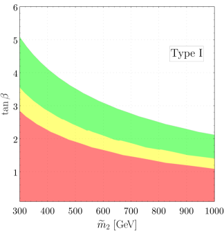
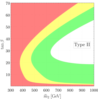
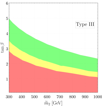
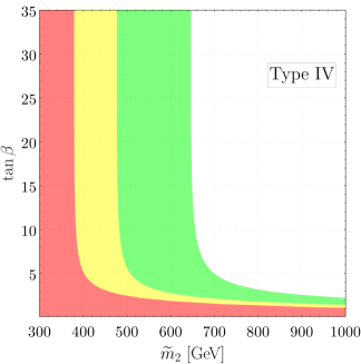
Figure 1: Bounds given by flavour observables in Tab. 1 for the different types of 2HDM. The green(yellow)[red] area corresponds to [1โ€‹ฯƒ,2โ€‹ฯƒ]1๐œŽ2๐œŽ[1\sigma,2\sigma]([2โ€‹ฯƒ,3โ€‹ฯƒ]2๐œŽ3๐œŽ[2\sigma,3\sigma])[>3โ€‹ฯƒabsent3๐œŽ>3\sigma] region.

The complete list of observables used in our fit is shown in Tab. 1. The plots referring to Type I and Type III are very similar to each other, excluding only the low values of tanโกฮฒ๐›ฝ\tan\beta, mainly due to โ„ฌโ€‹(Bโ†’Xsโ€‹ฮณ)โ„ฌโ†’๐ตsubscript๐‘‹๐‘ ๐›พ\mathcal{B}(B\to X_{s}\gamma), ฮ”โ€‹MBsฮ”subscript๐‘€subscript๐ต๐‘ \Delta M_{B_{s}} and Bd,sโ†’ฮผ+โ€‹ฮผโˆ’โ†’subscript๐ต๐‘‘๐‘ superscript๐œ‡superscript๐œ‡B_{d,s}\to\mu^{+}\mu^{-}. The plot for Type IV shows, on top of the aforementioned limit for low tanโกฮฒ๐›ฝ\tan\beta values, a strong cut on low m~2subscript~๐‘š2\widetilde{m}_{2} for any values of tanโกฮฒ๐›ฝ\tan\beta, mainly constrained by the rare radiative B๐ตB decay. Finally, the most constrained parameter space is the one of Type II, where smallish and largish values of tanโกฮฒ๐›ฝ\tan\beta are disfavoured even for large m~2subscript~๐‘š2\widetilde{m}_{2}. While โ„ฌโ€‹(Bโ†’Xsโ€‹ฮณ)โ„ฌโ†’๐ตsubscript๐‘‹๐‘ ๐›พ\mathcal{B}(B\to X_{s}\gamma) is the main responsible for the lower bound on m~2subscript~๐‘š2\widetilde{m}_{2}, the large tanโกฮฒ๐›ฝ\tan\beta region is mostly constrained by Bsโ†’ฮผ+โ€‹ฮผโˆ’โ†’subscript๐ต๐‘ superscript๐œ‡superscript๐œ‡B_{s}\to\mu^{+}\mu^{-}. For intermediate values of tanโกฮฒ๐›ฝ\tan\beta, the lower bound on m~2subscript~๐‘š2\widetilde{m}_{2} is similar to the one for the Type IV scenario. This result follows mainly from the constraints given by the combination of the rates for the radiative B๐ตB decay and for the leptonic neutral B๐ตB decays.

The reason for those similarities and differences may be traced back to the tanโกฮฒ๐›ฝ\tan\beta and cotโกฮฒ๐›ฝ\cot\beta dependence of the Wilson coefficients Eq. (2.22), which also determine the loop effects for the different types of 2HDM. In turn, they depend on the Yukawa couplings. As the Higgs couplings with the up-type quarks always include cotโกฮฒ๐›ฝ\cot\beta, they do not play a role in differentiating among the different constructions. On the other hand, ฮถd=โˆ’tanโกฮฒsubscript๐œ๐‘‘๐›ฝ\zeta_{d}=-\tan\beta for Type II and Type IV and therefore โ„ฌโ€‹(Bโ†’Xsโ€‹ฮณ)โ„ฌโ†’๐ตsubscript๐‘‹๐‘ ๐›พ\mathcal{B}(B\to X_{s}\gamma) grows with larger tanโกฮฒ๐›ฝ\tan\beta values: wherein the Type IV plot, this translates in the almost vertical bound on m~2subscript~๐‘š2\widetilde{m}_{2} once tanโกฮฒ๐›ฝ\tan\beta is larger than โˆผ2similar-toabsent2\sim 2; in the Type II plot, instead, it corresponds to the bounds on m~2subscript~๐‘š2\widetilde{m}_{2} for intermediate tanโกฮฒ๐›ฝ\tan\beta values, that matches the limits aforementioned. This enhancement is absent in Type I and III as โ„ฌโ€‹(Bโ†’Xsโ€‹ฮณ)โ„ฌโ†’๐ตsubscript๐‘‹๐‘ ๐›พ\mathcal{B}(B\to X_{s}\gamma) is suppressed with tanโกฮฒ๐›ฝ\tan\beta. Finally, the differences between Type II and Type IV are mainly due to the Higgs couplings to the charged leptons that have an effect in the leptonic neutral B๐ตB decays: their branching ratios are enhanced with tanโกฮฒ๐›ฝ\tan\beta only for Type II and thus their bounds strongly constrain the parameter space.

The results presented above are overall in agreement with the literature, see e.g. Ref.s [120, 121, 122, 123]. One of the most updated references is Ref. [120], which however presents two relevant differences. First, the lower bound on m~2subscript~๐‘š2\widetilde{m}_{2} present in Type II and IV is about 100โ€‹GeV100GeV100\ \text{GeV} smaller in our case. The reason is mostly to be found in the inclusion of recent data of angular observables of B0โ†’Kโˆ—โ€‹ฮผ+โ€‹ฮผโˆ’โ†’subscript๐ต0superscript๐พโˆ—superscript๐œ‡superscript๐œ‡B_{0}\to K^{\ast}\mu^{+}\mu^{-}, as some of them show relatively large deviations from the SM predictions, even above 2โ€‹ฯƒ2๐œŽ2\sigma, e.g. P5โ€ฒsuperscriptsubscript๐‘ƒ5โ€ฒP_{5}^{\prime}. Secondly, according to Refs. [108, 120], in Type II the uppermost allowed value is tanโกฮฒโˆผ30similar-to๐›ฝ30\tan\beta\sim 30, which is a bound almost twice as strong as ours. Such bound is mainly due to Bsโ†’ฮผ+โ€‹ฮผโˆ’โ†’subscript๐ต๐‘ superscript๐œ‡superscript๐œ‡B_{s}\to\mu^{+}\mu^{-} and B+โ†’ฯ„+โ€‹ฮฝโ†’superscript๐ตsuperscript๐œ๐œˆB^{+}\to\tau^{+}\nu. The cause of the discrepancy could be one of the following reasons or a combination of them: i) a different treatment of the theoretical errors; ii) the fact that we do not let the masses of the different scalars float when doing the fit. Finally, our results for Type II are in excellent agreement with those of Ref. [123].

Apart from flavour observables, one could expect significant constraints from direct searches at collider. The most constraining ones regard the searches for heavy neutral particles. Such bounds typically are given only for specific types of Z2subscript๐‘2Z_{2}-models, especially for Type II. They depend on other parameters of the model besides m~2subscript~๐‘š2\widetilde{m}_{2} and tanโกฮฒ๐›ฝ\tan\beta, such as the mixing of the CP-even scalars, cosโก(ฮฒโˆ’ฮฑ)๐›ฝ๐›ผ\cos(\beta-\alpha), Eq. (2.12). Direct searches bounds can be relevant for โ‰ฒ400โ€‹GeVless-than-or-similar-toabsent400GeV\lesssim 400\ \text{GeV} [124], that is in a region of the parameter space where the near the decoupling limit starts to be problematic. For this reason, we will not report such bounds in the results of the following sections.

3.2 Electron electric dipole moment

The present experimental bound on the electric dipole moment (EDM) of the electron provided by the ACME II collaboration [125],

de=(4.3ยฑ3.1ยฑ2.6)ร—10โˆ’30โ€‹ e cmsubscript๐‘‘๐‘’plus-or-minus4.33.12.6superscript1030 e cmd_{e}=\left(4.3\pm 3.1\pm 2.6\right)\times 10^{-30}\text{ e cm} (3.3)

translated to an upper bound at 2โ€‹ฯƒ2๐œŽ2\sigma

|de|<1.24ร—10โˆ’29โ€‹ e cm,subscript๐‘‘๐‘’1.24superscript1029 e cm|d_{e}|<1.24\times 10^{-29}\text{ e cm}\,, (3.4)

represents one of the most powerful observables to constrain the CP-violating phases in NP models. Using the effective description in terms of the ฮบ๐œ…\kappa-formalism in Eq. (2.18), we can translate this limit into a bound on ฮบ~fsubscript~๐œ…๐‘“\widetilde{\kappa}_{f}, the imaginary parts in the Yukawa couplings accounting for the effects of the d=6๐‘‘6d=6 corrections.

Due to the correlations between ฮบ~fsubscript~๐œ…๐‘“\widetilde{\kappa}_{f}โ€™s emphasized in the previous section, the electron EDM depends to a very good approximation only on the parameter C~~๐ถ\widetilde{C} defined in Eq. (3.1) and the value of tanโกฮฒ๐›ฝ\tan\beta, which fixes the relative magnitudes of the three ฮบ~fsubscript~๐œ…๐‘“\widetilde{\kappa}_{f}โ€™s, for the up, down and charged lepton sectors. Ref. [126], which corrects the results given in Ref. [127], presents the explicit expression for desubscript๐‘‘๐‘’d_{e} in the limit we are discussing here, that is in Z2subscript๐‘2Z_{2}-symmetric 2HD models near the decoupling limit:

Type I: deโ‰ƒ1.06ร—10โˆ’27โ€‹|ฮป~6|โ€‹sinโก((ฯ))โ€‹(1โ€‹TeVm~2)2ร—cotโกฮฒโ€‹[1+0.07โ€‹lnโก(m~21โ€‹TeV)]โ€‹e cm,similar-to-or-equalssubscript๐‘‘๐‘’1.06superscript1027subscript~๐œ†6๐œŒsuperscript1TeVsubscript~๐‘š22๐›ฝdelimited-[]10.07subscript~๐‘š21TeVe cm\displaystyle d_{e}\simeq 1.06\times 10^{-27}\,\left|\widetilde{\lambda}_{6}\right|\sin{(\rho)}\left(\dfrac{1\ \text{TeV}}{\widetilde{m}_{2}}\right)^{2}\times\cot\beta\left[1+0.07\ln\left(\dfrac{\widetilde{m}_{2}}{1\ \text{TeV}}\right)\right]\text{e cm}\,, (3.5)
Type II: deโ‰ƒโˆ’0.47ร—10โˆ’27|ฮป~6|sinโก((ฯ))(1โ€‹TeVm~2)2ร—\displaystyle d_{e}\simeq-0.47\times 10^{-27}\,\left|\widetilde{\lambda}_{6}\right|\sin{(\rho)}\left(\dfrac{1\ \text{TeV}}{\widetilde{m}_{2}}\right)^{2}\times
ร—{tanโกฮฒโ€‹[1+0.16โ€‹lnโก(m~21โ€‹TeV)]โˆ’1.26โ€‹cotโกฮฒ}โ€‹e cm,absent๐›ฝdelimited-[]10.16subscript~๐‘š21TeV1.26๐›ฝe cm\displaystyle\hskip 85.35826pt\times\left\{\tan\beta\left[1+0.16\ln\left(\dfrac{\widetilde{m}_{2}}{1\ \text{TeV}}\right)\right]-1.26\cot\beta\right\}\text{e cm}\,,
Type III: deโ‰ƒโˆ’0.47ร—10โˆ’27|ฮป~6|sinโก((ฯ))(1โ€‹TeVm~2)2ร—\displaystyle d_{e}\simeq-0.47\times 10^{-27}\,\left|\widetilde{\lambda}_{6}\right|\sin{(\rho)}\left(\dfrac{1\ \text{TeV}}{\widetilde{m}_{2}}\right)^{2}\times
ร—{tanโกฮฒโ€‹[1+0.16โ€‹lnโก(m~21โ€‹TeV)]โˆ’1.25โ€‹cotโกฮฒ}โ€‹e cm,absent๐›ฝdelimited-[]10.16subscript~๐‘š21TeV1.25๐›ฝe cm\displaystyle\hskip 85.35826pt\times\left\{\tan\beta\left[1+0.16\ln\left(\dfrac{\widetilde{m}_{2}}{1\ \text{TeV}}\right)\right]-1.25\cot\beta\right\}\text{e cm}\,,
Type IV: deโ‰ƒ1.06ร—10โˆ’27|ฮป~6|sinโก((ฯ))(1โ€‹TeVm~2)2ร—\displaystyle d_{e}\simeq 1.06\times 10^{-27}\,\left|\widetilde{\lambda}_{6}\right|\sin{(\rho)}\left(\dfrac{1\ \text{TeV}}{\widetilde{m}_{2}}\right)^{2}\times
ร—{cotโกฮฒโ€‹[1+0.07โ€‹lnโก(m~21โ€‹TeV)]+0.002โ€‹tanโกฮฒ}โ€‹e cm.absent๐›ฝdelimited-[]10.07subscript~๐‘š21TeV0.002๐›ฝe cm\displaystyle\hskip 85.35826pt\times\left\{\cot\beta\left[1+0.07\ln\left(\dfrac{\widetilde{m}_{2}}{1\ \text{TeV}}\right)\right]+0.002\tan\beta\right\}\text{e cm}\,.

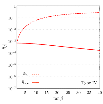
We use the above equations to find upper bounds of C~~๐ถ\widetilde{C} as a function of tanโกฮฒ๐›ฝ\tan\beta for each Type of the model: these limits are approximately independent from m~2subscript~๐‘š2\widetilde{m}_{2}, as the m~2subscript~๐‘š2\widetilde{m}_{2}-dependent logarithmic terms are numerically negligible in the considered range of m~2subscript~๐‘š2\widetilde{m}_{2}. Then, using Eqs. (2.18) one obtains upper bounds on the imaginary parts of the Yukawas shown in Fig. 2. They are shown for Type II and IV. For Type I the upper bounds for all 3 ฮบ~fsubscript~๐œ…๐‘“\widetilde{\kappa}_{f}โ€™s are the same, of order 10โˆ’3superscript10310^{-3}; for Type III the bound on ฮบ~esubscript~๐œ…๐‘’\widetilde{\kappa}_{e} remains as for Type II and the bound on ฮบ~dsubscript~๐œ…๐‘‘\widetilde{\kappa}_{d} is the same as the bound on ฮบ~usubscript~๐œ…๐‘ข\widetilde{\kappa}_{u} in Type II. This behaviour can be easily understood from Eqs. (2.18).
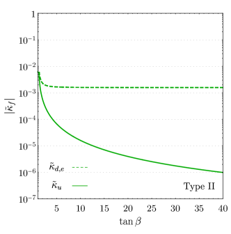
Refer to caption
(a) Type II
Refer to caption
(b) Type IV
Figure 2: Upper bounds on ฮบ~fsubscript~๐œ…๐‘“\widetilde{\kappa}_{f} at 95% C.L. for Type II and IV.

It is worth commenting on the structure of the bounds in the context of experimental search for various CP-sensitive asymmetries in the Higgs production and decays. At least in the framework of the Z2subscript๐‘2Z_{2} symmetric 2HDMs, the search for such effects in the hโ€‹tโ€‹tโ„Ž๐‘ก๐‘กhtt coupling is least promising. Better chances are offered by the down quark sector in Type IV, but otherwise, the limits are always very strong, at the level of ฮบ~fโ‰ˆ10โˆ’2โˆ’10โˆ’3subscript~๐œ…๐‘“superscript102superscript103\widetilde{\kappa}_{f}\approx 10^{-2}-10^{-3}.

The individual fermion loop contributions in the Barr-Zee diagrams to the electron EDM, and therefore the role of each loop in getting the final upper bound for C~~๐ถ\tilde{C}, depend on the structure of the ฮถfsubscript๐œ๐‘“\zeta_{f} coefficients in Eqs. (2.18) and on the fermion masses, which enter into the loop calculation. For the Type I case, for example, all ฮบ~fsubscript~๐œ…๐‘“\widetilde{\kappa}_{f}โ€™s are weighted by cotโกฮฒ๐›ฝ\cot\beta and one can see that the dominant contribution to desubscript๐‘‘๐‘’d_{e} comes from the top loop (see the discussion in Ref. [49], where the analysis considering only one NP parameter at a time was performed). Differently, for the Type II and Type III, the charged lepton contributions are enhanced by tanโกฮฒ๐›ฝ\tan\beta, and thus the bound can be directly associated with them. Finally, for type IV, it depends on the value of tanโกฮฒ๐›ฝ\tan\beta that only enhances the down-type quarks.

It is also worth mentioning the possible cancellation that could take place for specific values of tanโกฮฒ๐›ฝ\tan\beta between the terms in the curly brackets of the previous expressions. Interestingly, the same pattern of relations also holds for the neutron EDM, but with different numerical factors. As a result, even if one may select a specific value for tanโกฮฒ๐›ฝ\tan\beta that cancels the NP contributions to the electron EDM, the bounds from the neutron EDM would still apply, providing a smaller but still strong constraint on the ฮบ~fsubscript~๐œ…๐‘“\widetilde{\kappa}_{f}.

Refer to caption
(a)
Refer to caption
(b)
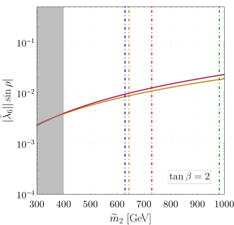
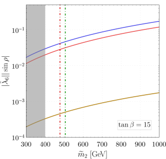
Figure 3: Upper bounds at 2โ€‹ฯƒ2๐œŽ2\sigma from electron EDM for different types of 2HDM and values of tanโกฮฒ๐›ฝ\tan\beta. Each colour corresponds to a specific realisation of 2HDM: Type I-blue, Type II-green, Type III-orange, Type IV-red. The plot is symmetric with respect to the x-axis for negative values of ฯ๐œŒ\rho. The area on the left-side of the vertical dot-dashed lines is excluded at 2โ€‹ฯƒ2๐œŽ2\sigma by flavour observables. In the grey shaded area the v/m~2๐‘ฃsubscript~๐‘š2v/\widetilde{m}_{2} expansion is not precise and can be affected by โ‰ณ๐’ชโ€‹(40%)greater-than-or-equivalent-toabsent๐’ชpercent40\gtrsim\mathcal{O}(40\%) corrections.

It is useful to show the upper bound on the parameter C~~๐ถ\widetilde{C} as the bound on the parameter |ฮป~6|โ€‹sinโก(ฯ)subscript~๐œ†6๐œŒ|\widetilde{\lambda}_{6}|\sin{\rho} as a function of m~2subscript~๐‘š2\widetilde{m}_{2} (the logarithmic terms are included). The results are shown in Fig. 3. The four plots refers to different values of tanโกฮฒ={2,โ€‰15}๐›ฝ215\tan\beta=\{2,\,15\}, and the lines are the 2โ€‹ฯƒ2๐œŽ2\sigma upper bounds on |ฮป~6|โ€‹sinโกฯsubscript~๐œ†6๐œŒ|\widetilde{\lambda}_{6}|\sin\rho as a function of m~2subscript~๐‘š2\widetilde{m}_{2}. The colours identify the 2HDM construction: Type I-blue, Type II-green, Type III-orange, Type IV-red. The vertical lines are the 2โ€‹ฯƒ2๐œŽ2\sigma lower bounds for m~2subscript~๐‘š2\widetilde{m}_{2} as identified in Fig. 1 from the fit with data from the flavour observables in Tab. 1. The values on the left of these lines are therefore excluded.

With analogous results for |ฮป~6|โ€‹cosโก(ฯ)subscript~๐œ†6๐œŒ|\widetilde{\lambda}_{6}|\cos{\rho} as a function of m~2subscript~๐‘š2\widetilde{m}_{2} obtained in the next subsection, one can infer the acceptable values for the coupling |ฮป~6|subscript~๐œ†6|\widetilde{\lambda}_{6}| and the phase ฯ๐œŒ\rho, separately.

3.3 Collider Observables

In this section we investigate the bounds on the real parts of the Yukawa couplings following from the Higgs boson production and decay data. We employ the latest results from ATLAS [128] and CMS [129]. The experimental data can be used to constrain the parameters ฮบVsubscript๐œ…๐‘‰\kappa_{V} describing the deviations from the SM predictions of the Higgs couplings to gauge bosons, defined in Eq. (LABEL:eq:kappaVV), and the combinations

rf2โ‰กฮบf2+ฮบ~f2,superscriptsubscript๐‘Ÿ๐‘“2superscriptsubscript๐œ…๐‘“2superscriptsubscript~๐œ…๐‘“2r_{f}^{2}\equiv\kappa_{f}^{2}+\widetilde{\kappa}_{f}^{2}\,, (3.6)

with ฮบfsubscript๐œ…๐‘“\kappa_{f} and ฮบ~fsubscript~๐œ…๐‘“\widetilde{\kappa}_{f} in Eq. (2.18), for the couplings with fermions. The results reported by the experimental collaborations are shown in Tab. 2.

ATLAS [128] CMS [129]
rฮผsubscript๐‘Ÿ๐œ‡r_{\mu} 1.07โ€‹(26)1.07261.07(26) 1.11โ€‹(21)1.11211.11(21)
rฯ„subscript๐‘Ÿ๐œr_{\tau} 0.94โ€‹(7)0.9470.94(7) 0.925โ€‹(75)0.925750.925(75)
rbsubscript๐‘Ÿ๐‘r_{b} 0.90โ€‹(11)0.90110.90(11) 1.02โ€‹(16)1.02161.02(16)
rtsubscript๐‘Ÿ๐‘กr_{t} 0.95โ€‹(7)0.9570.95(7) 0.95โ€‹(7)0.9570.95(7)
ฮบWsubscript๐œ…๐‘Š\kappa_{W} 1.02โ€‹(5)1.0251.02(5) 1.03โ€‹(3)1.0331.03(3)
ฮบZsubscript๐œ…๐‘\kappa_{Z} 0.99โ€‹(6)0.9960.99(6) 1.02โ€‹(3)1.0231.02(3)
Table 2: Values of risubscript๐‘Ÿ๐‘–r_{i} and kVsubscript๐‘˜๐‘‰k_{V} used for the fits.

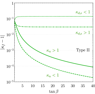
The EDM upper bounds at the 2โ€‹ฯƒ2๐œŽ2\sigma level for the ฮบ~fsubscript~๐œ…๐‘“\widetilde{\kappa}_{f}โ€™s are significantly stronger than the uncertainties on the rfsubscript๐‘Ÿ๐‘“r_{f}โ€™s shown (at 1โ€‹ฯƒ1๐œŽ1\sigma) in Tab. 2, so in our analysis of the bounds on the ฮบfsubscript๐œ…๐‘“\kappa_{f}โ€™s we assume ฮบ~f=0subscript~๐œ…๐‘“0\widetilde{\kappa}_{f}=0. The accuracy of this approximation can be judged once the results for the bounds on ฮบ๐œ…\kappaโ€™s are obtained. Thus, taking rf=ฮบfsubscript๐‘Ÿ๐‘“subscript๐œ…๐‘“r_{f}=\kappa_{f}, we fit the parameter C๐ถC defined in Eq. (3.1). For each value of tanโกฮฒ๐›ฝ\tan\beta, we define a ฯ‡2superscript๐œ’2\chi^{2}-function based on the data on rfsubscript๐‘Ÿ๐‘“r_{f} and we obtain the best-fit value of C๐ถC for each type of the model. In each case, the results of the fit are most sensitive to those rfsubscript๐‘Ÿ๐‘“r_{f}โ€™s in Tab. 2 for which ฮถf=tanโกฮฒsubscript๐œ๐‘“๐›ฝ\zeta_{f}=\tan\beta. Next, using Eqs. (2.18) with fitted values for C๐ถC, we obtain the bounds shown at 2โ€‹ฯƒ2๐œŽ2\sigma level in Fig. 4 for Type II and IV.

Refer to caption
(a)
Refer to caption
(b)
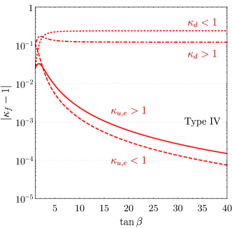
Figure 4: Upper and lower bounds on ฮบfsubscript๐œ…๐‘“\kappa_{f} at 95% C.L. for Type II and IV.

As it follows from Eqs. (2.18), for Type I the bounds are tanโกฮฒ๐›ฝ\tan\beta independent and the same for all ฮบfsubscript๐œ…๐‘“\kappa_{f}โ€™s in the range

0.9<ฮบf<1.02,0.9subscript๐œ…๐‘“1.020.9<\kappa_{f}<1.02\,, (3.7)

For Type III, ฮบd=ฮบusubscript๐œ…๐‘‘subscript๐œ…๐‘ข\kappa_{d}=\kappa_{u} and ฮบesubscript๐œ…๐‘’\kappa_{e} remains as in Type II. We see that in most cases ฮบfโ‰ซฮบ~fmuch-greater-thansubscript๐œ…๐‘“subscript~๐œ…๐‘“\kappa_{f}\gg\widetilde{\kappa}_{f}, consistently with our approximation. Similarly as for the EDM bounds, we note that the structure of correlations for the Yukawa couplings predicted by the models results in very strong bounds on the hโ€‹tโ€‹tโ„Ž๐‘ก๐‘กhtt coupling. For seeing the deviations from the SM, the Higgs decays to the down quarks and leptons (for Type II), only to leptons (Type III) and only to the down quarks (Type IV) are much more promising.

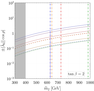
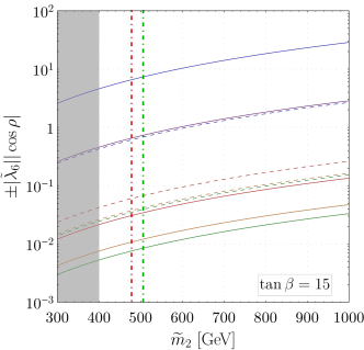
The best fit results obtained for the parameters C๐ถC translate into parabola-like branches in the parameter space |ฮป~6|โ€‹cosโก((ฯ))subscript~๐œ†6๐œŒ|\widetilde{\lambda}_{6}|\cos{(\rho)} vs. m~2subscript~๐‘š2\widetilde{m}_{2}. The results are shown in Fig. 5 for different values of tanโกฮฒ={2,โ€‰15}๐›ฝ215\tan\beta=\{2,\,15\}. The lines represent the 2โ€‹ฯƒ2๐œŽ2\sigma upper limit on the combination |ฮป~6|โ€‹|cosโก((ฯ))|subscript~๐œ†6๐œŒ|\widetilde{\lambda}_{6}|\left|\cos{(\rho)}\right|: solid (dot-dashed) lines correspond to positive (negative) values of cosโก((ฯ))๐œŒ\cos{(\rho)}. As for Fig. 3, the colours identify the 2HDM construction, that is Type I-blue, Type II-green, Type III-orange, Type IV-red. Moreover, the vertical lines are again the 2โ€‹ฯƒ2๐œŽ2\sigma lower bounds for m~2subscript~๐‘š2\widetilde{m}_{2} as identified in Fig. 1.

Refer to caption
(a)
Refer to caption
(b)
Figure 5: Upper bounds at 2โ€‹ฯƒ2๐œŽ2\sigma from collider observables for different types of 2HDM and values of tanโกฮฒ๐›ฝ\tan\beta. Each colour corresponds to a specific realisation of 2HDM: Type I-blue, Type II-green, Type III-orange, Type IV-red. The case with cosโกฯ>0(<0)๐œŒannotated0absent0\cos\rho>0\leavevmode\nobreak\ (<0) corresponds to solid (dashed) lines. The area on the left-side of the vertical dot-dashed lines is excluded at 2โ€‹ฯƒ2๐œŽ2\sigma by flavour observables. The purple line corresponds to the limit in Eq. (3.9) and it applies to the case |cosโกฯ|=1๐œŒ1\left|\cos\rho\right|=1. In the grey shaded area the v/m~2๐‘ฃsubscript~๐‘š2v/\widetilde{m}_{2} expansion is not precise and can be affected by โ‰ณ๐’ชโ€‹(40%)greater-than-or-equivalent-toabsent๐’ชpercent40\gtrsim\mathcal{O}(40\%) corrections.

As the value of tanโกฮฒ๐›ฝ\tan\beta grows, larger values for |ฮป~6|โ€‹|cosโก((ฯ))|subscript~๐œ†6๐œŒ|\widetilde{\lambda}_{6}|\left|\cos{(\rho)}\right| are allowed in the Type I 2HDM case, while the contrary holds for the other cases. This is easy to understand for the Type I 2HDM, where ฮถu,d,e=cotโกฮฒsubscript๐œ๐‘ข๐‘‘๐‘’๐›ฝ\zeta_{u,d,e}=\cot\beta, and then the fitted values of the parameter C๐ถC increase with larger tanโกฮฒ๐›ฝ\tan\beta. On the other hand, the analysis is more involved for the other constructions: indeed, it is the combination of the sensitivity to the different rfsubscript๐‘Ÿ๐‘“r_{f} and the dependence on tanโกฮฒ๐›ฝ\tan\beta or cotโกฮฒ๐›ฝ\cot\beta that determines which is the dominant contribution in the fit.

Comparing Figs. 3 and 5, we can conclude that generically |ฮป~6|โ€‹|cosโก((ฯ))|โ‰ซ|ฮป~6|โ€‹|sinโก((ฯ))|much-greater-thansubscript~๐œ†6๐œŒsubscript~๐œ†6๐œŒ|\widetilde{\lambda}_{6}|\left|\cos{(\rho)}\right|\gg\left|\widetilde{\lambda}_{6}\right|\left|\sin{(\rho)}\right|. This confirms once again the validity of the approximation chosen in the fit with only the fermionic collider data and can be interpreted as |cosโกฯ|โ‰ˆ1๐œŒ1\left|\cos\rho\right|\approx 1. In fact, generically the bounds on |ฮป~6|โ€‹|cosโก((ฯ))|subscript~๐œ†6๐œŒ|\widetilde{\lambda}_{6}|\left|\cos{(\rho)}\right| are ๐’ชโ€‹(10โˆ’100)๐’ช10100\mathcal{O}(10-100) stronger than the ones on |ฮป~6|โ€‹|sinโก((ฯ))|subscript~๐œ†6๐œŒ|\widetilde{\lambda}_{6}|\left|\sin{(\rho)}\right|. The only exception lies in Type IV, as the two upper bounds become of the same order for tanโกฮฒโˆผ15similar-to๐›ฝ15\tan\beta\sim 15. Eventually, for larger values of tanโกฮฒ๐›ฝ\tan\beta, the bound on |ฮป~6|โ€‹|sinโก((ฯ))|subscript~๐œ†6๐œŒ|\widetilde{\lambda}_{6}|\left|\sin{(\rho)}\right| become weaker than the one of |ฮป~6|โ€‹|cosโก((ฯ))|subscript~๐œ†6๐œŒ|\widetilde{\lambda}_{6}|\left|\cos{(\rho)}\right|. One should thus expect corrections of ๐’ชโ€‹(1)๐’ช1\mathcal{O}(1) which, however, should not change the magnitude of the limits.

On the other hand, some care is necessary when considering the large tanโกฮฒ๐›ฝ\tan\beta scenario, as the bounds are relatively weak and |ฮป~6|subscript~๐œ†6|\widetilde{\lambda}_{6}| could reach values as large as m~22/v2superscriptsubscript~๐‘š22superscript๐‘ฃ2\widetilde{m}_{2}^{2}/v^{2}, that are inconsistent with the decoupling limit. This is already the case for tanโกฮฒ=15๐›ฝ15\tan\beta=15 and for m~22โ‰ณ850โ€‹GeVgreater-than-or-equivalent-tosuperscriptsubscript~๐‘š22850GeV\widetilde{m}_{2}^{2}\gtrsim 850\ \text{GeV}: in this case, the upper bound on |ฮป~6|subscript~๐œ†6|\widetilde{\lambda}_{6}| should be read from Eq. (2.11).

Finally, performing a fit including only ฮบWsubscript๐œ…๐‘Š\kappa_{W} and ฮบZsubscript๐œ…๐‘\kappa_{Z} from both collaborations, where

ฮบV=subscript๐œ…๐‘‰absent\displaystyle\kappa_{V}= 1โˆ’12โ€‹|ฮป~6|2โ€‹(v2m~22)2,112superscriptsubscript~๐œ†62superscriptsuperscript๐‘ฃ2superscriptsubscript~๐‘š222\displaystyle 1-\dfrac{1}{2}\left|\widetilde{\lambda}_{6}\right|^{2}\left(\dfrac{v^{2}}{\widetilde{m}_{2}^{2}}\right)^{2}\,, (3.8)

we obtain at 2โ€‹ฯƒ2๐œŽ2\sigma

|ฮป~6|โ€‹(v2m~22)โ‰ค0.17.subscript~๐œ†6superscript๐‘ฃ2superscriptsubscript~๐‘š220.17\left|\widetilde{\lambda}_{6}\right|\left(\dfrac{v^{2}}{\widetilde{m}_{2}^{2}}\right)\leq 0.17\,. (3.9)

This result is valid for all four types of 2HDM realisations and is independent of tanโกฮฒ๐›ฝ\tan\beta. We show this limit in Fig. 5 as an additional purple line. Although strictly speaking, this line refers only to the case with cosโกฯ=1๐œŒ1\cos\rho=1, it helps to guide the eye in the interpretation of the relative magnitude of the different bounds.

3.4 Triple Higgs Coupling

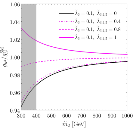
With the results of the previous sections for the bounds on the mass scale m~2subscript~๐‘š2{\tilde{m}}_{2} and the coupling ฮป~6subscript~๐œ†6{\widetilde{\lambda}}_{6}, in this section we discuss the triple Higgs coupling, whose deviation from the SM is reported in Eq. (2.20). The latest bounds on it are given by the ATLAS collaboration [130] and read (at 2โ€‹ฯƒ2๐œŽ2\sigma)

โˆ’1.4<gh3gh3SM<6.1.1.4subscript๐‘”superscriptโ„Ž3superscriptsubscript๐‘”superscriptโ„Ž3SM6.1-1.4<\dfrac{g_{h^{3}}}{g_{h^{3}}^{\text{SM}}}<6.1\,. (3.10)

The leading NP contribution depends on the ratio |ฮป~6|2โ€‹v2/m~22superscriptsubscript~๐œ†62superscript๐‘ฃ2superscriptsubscript~๐‘š22|\widetilde{\lambda}_{6}|^{2}v^{2}/\widetilde{m}_{2}^{2}. It depends on tanโกฮฒ๐›ฝ\tan\beta through the values of ฮป~6subscript~๐œ†6{\widetilde{\lambda}}_{6}. One then generically expects that, even considering the largest allowed values on |ฮป~6|โ€‹|cosโก((ฯ))|subscript~๐œ†6๐œŒ|\widetilde{\lambda}_{6}|\left|\cos{(\rho)}\right| and |ฮป~6|โ€‹|sinโก((ฯ))|subscript~๐œ†6๐œŒ|\widetilde{\lambda}_{6}|\left|\sin{(\rho)}\right| determined in the previous sections, the predicted deviation from the SM of gh3subscript๐‘”superscriptโ„Ž3g_{h^{3}} is smaller than the direct bound in Eq. (3.10) (see for example Refs. [131, 132, 133, 134, 135, 136]).

It is well known that the radiative corrections to the triple Higgs coupling are relevant. Focussing on the 1โˆ’limit-from11-loop contributions in the CP conserving limit, that is a good approximation given the smallness of the CP violating phases as shown in the previous sections, we can write [137],

gh3=gh3Tโ€‹L+ฮดโ€‹gh3,subscript๐‘”superscriptโ„Ž3subscriptsuperscript๐‘”๐‘‡๐ฟsuperscriptโ„Ž3๐›ฟsubscript๐‘”superscriptโ„Ž3g_{h^{3}}=g^{TL}_{h^{3}}+\delta g_{h^{3}}\,, (3.11)

where gh3Tโ€‹Lsubscriptsuperscript๐‘”๐‘‡๐ฟsuperscriptโ„Ž3g^{TL}_{h^{3}} is given in Eq. (2.20) while ฮดโ€‹gh3๐›ฟsubscript๐‘”superscriptโ„Ž3\delta g_{h^{3}} reads

ฮดโ€‹gh3โ‰ˆ๐›ฟsubscript๐‘”superscriptโ„Ž3absent\displaystyle\delta g_{h^{3}}\approx 3โ€‹mh2v2{112โ€‹ฯ€2โ€‹mh2โ€‹v2[mH4(1โˆ’m~22mH2)3+mA4(1โˆ’m~22mA2)3]\displaystyle\dfrac{3m_{h}^{2}}{v^{2}}\left\{\dfrac{1}{12\pi^{2}m_{h}^{2}v^{2}}\left[m_{H}^{4}\left(1-\dfrac{\widetilde{m}_{2}^{2}}{m_{H}^{2}}\right)^{3}+m_{A}^{4}\left(1-\dfrac{\widetilde{m}_{2}^{2}}{m_{A}^{2}}\right)^{3}\right]\right. (3.12)
+mHยฑ46โ€‹ฯ€2โ€‹mh2โ€‹v2(1โˆ’m~22mHยฑ2)3โˆ’Ncโ€‹mt43โ€‹ฯ€2โ€‹mh2โ€‹v2},\displaystyle\hskip 42.67912pt\left.+\dfrac{m_{H_{\pm}}^{4}}{6\pi^{2}m_{h}^{2}v^{2}}\left(1-\dfrac{\widetilde{m}_{2}^{2}}{m_{H_{\pm}}^{2}}\right)^{3}-\dfrac{N_{c}m_{t}^{4}}{3\pi^{2}m_{h}^{2}v^{2}}\right\}\,,

where the last term is due to the SM contribution mediated by the top quark.

As can be seen, the contribution can be large if the decoupling is not realized or if the masses are not almost degenerate. In the case of almost decoupling, substituting the explicit expressions for the masses and keeping the leading contributions, the part containing the NP-corrections at 111-loop simplifies and reads

ฮดโ€‹gh3NPโ‰ˆ116โ€‹ฯ€2โ€‹(vm~2)2โ€‹[(ฮป~3+ฮป~4+ฮป~5)3+(ฮป~3โˆ’3โ€‹ฮป~5โ€‹(ฮป~3+ฮป~4)2โˆ’ฮป~53)].๐›ฟsuperscriptsubscript๐‘”superscriptโ„Ž3NP116superscript๐œ‹2superscript๐‘ฃsubscript~๐‘š22delimited-[]superscriptsubscript~๐œ†3subscript~๐œ†4subscript~๐œ†53superscript~๐œ†33subscript~๐œ†5superscriptsubscript~๐œ†3subscript~๐œ†42superscriptsubscript~๐œ†53\delta g_{h^{3}}^{\text{NP}}\approx\dfrac{1}{16\pi^{2}}\left(\dfrac{v}{\widetilde{m}_{2}}\right)^{2}\left[(\widetilde{\lambda}_{3}+\widetilde{\lambda}_{4}+\widetilde{\lambda}_{5})^{3}+(\widetilde{\lambda}^{3}-3\widetilde{\lambda}_{5}(\widetilde{\lambda}_{3}+\widetilde{\lambda}_{4})^{2}-\widetilde{\lambda}_{5}^{3})\right]\,. (3.13)

Notice that they are of the same order of magnitude as the leading corrections in Eq. (2.20) to the tree level result. Moreover, if ฮป~isubscript~๐œ†๐‘–\widetilde{\lambda}_{i} are positive, they may induce destructive interference with the tree-level NP contribution. Notably, the dependence on ฮป~3,4,5subscript~๐œ†345\widetilde{\lambda}_{3,4,5} scales with the third power, so the relative importance between tree- and loop-level contributions highly depends on such couplings. Such dependence is illustrated in Fig. 6 for ฮป~6=0.1subscript~๐œ†60.1\widetilde{\lambda}_{6}=0.1 and different values of ฮป~3,4,5subscript~๐œ†345\widetilde{\lambda}_{3,4,5}. To maximize the effect, we take ฮป~3=ฮป~4=ฮป~5subscript~๐œ†3subscript~๐œ†4subscript~๐œ†5\widetilde{\lambda}_{3}=\widetilde{\lambda}_{4}=\widetilde{\lambda}_{5}.

Refer to caption
Figure 6: Relative importance of the loop- vs. tree-level NP contributions. In the vertical axis we plot the ratio between the triple Higgs coupling prediction including NP contributions and the purely SM quantity at 1โˆ’limit-from11-loop level. The solid-black line only contains the tree-level NP contributions, while the purple lines also contain the 1โˆ’limit-from11-loop level NP contributions for different values of ฮป~3=ฮป~4=ฮป~5subscript~๐œ†3subscript~๐œ†4subscript~๐œ†5\widetilde{\lambda}_{3}=\widetilde{\lambda}_{4}=\widetilde{\lambda}_{5}.

One may expect that the parameters in the potential are of the same order of magnitude: for this reason and in order to simplify the discussion, without any loss of generality, in what follows we shall consider that ฮป~3,4,5subscript~๐œ†345\widetilde{\lambda}_{3,4,5} are close enough to ฮป~6subscript~๐œ†6\widetilde{\lambda}_{6} in order to neglect all NP contributions at 111-loop.

We combine the information from the electron EDM and collider Higgs data of the previous sections to determine an upper bound on |ฮป~6|2โ€‹v2/m~22superscriptsubscript~๐œ†62superscript๐‘ฃ2superscriptsubscript~๐‘š22|\widetilde{\lambda}_{6}|^{2}v^{2}/\widetilde{m}_{2}^{2}, summing quadratically the upper values for the real (โˆcosโกฯproportional-toabsent๐œŒ\propto\cos\rho) and imaginary (โˆsinโกฯproportional-toabsent๐œŒ\propto\sin\rho) parts, for any 2HDM realisations. With this procedure, we always obtain the strongest bound on the triple coupling as a function of m~2subscript~๐‘š2{\tilde{m}}_{2}, except for the Type I 2HDM. In the latter case, the strongest bound coincides with Eq. (3.9) (for the values of tanโกฮฒ>1๐›ฝ1\tan\beta>1). In Fig. 7 we show 2โ€‹ฯƒ2๐œŽ2\sigma the lower bounds on gh3/gh3SMsubscript๐‘”superscriptโ„Ž3superscriptsubscript๐‘”superscriptโ„Ž3SMg_{h^{3}}/g_{h^{3}}^{\text{SM}}, for tanโกฮฒ={2,โ€‰15}๐›ฝ215\tan\beta=\{2,\,15\}. We use the same colour code as the previous plots. The vertical lines are again the 2โ€‹ฯƒ2๐œŽ2\sigma lower bounds for m~2subscript~๐‘š2\widetilde{m}_{2} as identified in Fig. 1. Finally, the grey shaded area corresponds to the direct bound in Eq. (3.10). When the purple and blue lines do not appear they are outside the scale of the plots (they give much weaker bounds).
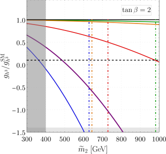
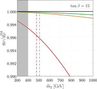
Refer to caption
(a)
Refer to caption
(b)
Figure 7: Lower bounds on triple Higgs-coupling normalised to the SM (tree- and 1โˆ’limit-from11-loop contribution) from collider observables for different types of 2HDM and values of tanโกฮฒ๐›ฝ\tan\beta. The solid black line corresponds to the SM prediction. Each colour corresponds to a specific realisation of 2HDM: Type I-blue, Type II-green, Type III-orange, Type IV-red. The purple line shows the universal bound from Higgs decay into gauge bosons in Eq. (3.9). Only the area enclosed within the coloured and black solid lines is allowed. The shaded grey area is excluded at 2โ€‹ฯƒ2๐œŽ2\sigma for all models from the direct measurement of the triple Higgs coupling. Finally, the area on the left-side of the vertical lines is excluded at 2โ€‹ฯƒ2๐œŽ2\sigma by flavour observables. In the grey shaded area the v/m~2๐‘ฃsubscript~๐‘š2v/\widetilde{m}_{2} expansion is not precise and can be affected by โ‰ณ๐’ชโ€‹(40%)greater-than-or-equivalent-toabsent๐’ชpercent40\gtrsim\mathcal{O}(40\%) corrections. The horizontal black dashed line corresponds to the lower value that HL-LHC will be able to probe at 95%percent9595\%C.L..

For Type II and Type III, the models predict very small deviations from the SM for the triple Higgs couplings, for any values of tanโกฮฒ๐›ฝ\tan\beta. This is also true for Type IV for larger values of tanโกฮฒ๐›ฝ\tan\beta. On the other hand, the Type IV 2HDM for smaller tanโกฮฒ๐›ฝ\tan\beta and the Type I for any tanโกฮฒ๐›ฝ\tan\beta values sizeable deviations are allowed and can be probed in the future colliders.

Finally, HL-LHC prospects to measure much more precisely such quantity. The current projections estimate to test gh3/gh3SMโˆˆ[0.1,2.3]subscript๐‘”superscriptโ„Ž3superscriptsubscript๐‘”superscriptโ„Ž3SM0.12.3g_{h^{3}}/g_{h^{3}}^{\text{SM}}\in[0.1,2.3] at 95%percent9595\% C.L. [138]. This remarkable improvement will be very useful to constrain Type-I, but it will not restrict the parameter space for the other types with respect to the current bounds from Higgs-fermion interactions.

3.5 ๐’Ž๐‘พsubscript๐’Ž๐‘พm_{W} from CDF II

The determination of the W-boson mass, ๐’Ž๐‘พsubscript๐’Ž๐‘พm_{W}, represents the last relevant anomaly in particle physics. The CDF II collaboration [17] measured it with the best-achieved sensitivity,

๐’Ž๐‘พCDF II=80.4335ยฑ0.0094โ€‹GeV,superscriptsubscript๐’Ž๐‘พCDF IIplus-or-minus80.43350.0094GeVm_{W}^{\text{CDF II}}=80.4335\pm 0.0094\ \text{GeV}\,, (3.14)

showing a ๐Ÿ•โ€‹๐ˆ7๐ˆ7\sigma discrepancy relative to the SM prediction [139]

๐’Ž๐‘พSM=80.354ยฑ0.007โ€‹GeV.superscriptsubscript๐’Ž๐‘พSMplus-or-minus80.3540.007GeVm_{W}^{\text{SM}}=80.354\pm 0.007\ \text{GeV}\,. (3.15)

Interestingly, this measure is not only in tension with the SM but also with all the other experimental determinations: the last one, from the ATLAS collaboration [18], shows no deviation from the SM prediction, although the uncertainties are not as good as those of the CDF II measurement.

We refrain here from taking a definite point of view and instead discuss under which conditions the 2HDM setup we discussed so far can agree either with the SM prediction or with the experimental CDF II result222As reported in Ref. [140], neglecting the possible correlations, one could estimate the average among the different experimental determinations obtaining a value for mwsubscript๐‘š๐‘คm_{w} only 1โ€‹ฯƒ1๐œŽ1\sigma far from the CDF II result, as expected. For this reason, we will perform our analysis considering the value in Eq. (1.1), understanding that the conclusions would remain invariant using instead the average quantity..

The most precise theoretical prediction of ๐’Ž๐‘พsubscript๐’Ž๐‘พm_{W} is obtained using ๐œถemsubscript๐œถem\alpha_{\text{em}}, ๐‘ฎ๐‘ญsubscript๐‘ฎ๐‘ญG_{F}, and ๐’Ž๐’๐Ÿsuperscriptsubscript๐’Ž๐’2m_{Z}^{2} as experimental input. As the Fermi constant is extracted experimentally from the dominant muon decay, if NP contributes to the branching ratio of this decay, then ๐‘ฎ๐‘ญsubscript๐‘ฎ๐‘ญG_{F} gets redefined and a tree-level modification of ๐’Ž๐‘พsubscript๐’Ž๐‘พm_{W} follows. However, the impact of 2HDM the dominant muon decay induced by the operators of Eq. (2.21) is extremely small, due to the suppression of the electron mass entering in the corresponding Wilson coefficients. It follows that no sizeable tree-level correction to the SM prediction is present.

Another possibility concerns the role of oblique corrections, and more specifically of the Peskin-Takeuchi parameters, ๐‘บ,๐‘ป,๐‘ผ๐‘บ๐‘ป๐‘ผS,T,U [141]. Denoted the loop-correction to the two-points function of the gauge fields ๐’Šโ€‹๐šท๐‘ฝโ€‹๐‘ฝ๐โ€‹๐‚โ‰ก๐’Šโ€‹๐šท๐‘ฝโ€‹๐‘ฝโ€‹๐œผ๐โ€‹๐‚+๐’Šโ€‹๐šท๐‘ฝโ€‹๐‘ฝ๐’‘โ€‹๐’‘โ€‹๐’‘๐โ€‹๐’‘๐‚๐’Šsubscriptsuperscript๐šท๐๐‚๐‘ฝ๐‘ฝ๐’Šsubscript๐šท๐‘ฝ๐‘ฝsuperscript๐œผ๐๐‚๐’Šsubscriptsuperscript๐šท๐’‘๐’‘๐‘ฝ๐‘ฝsuperscript๐’‘๐superscript๐’‘๐‚i\Pi^{\mu\nu}_{VV}\equiv i\Pi_{VV}\eta^{\mu\nu}+i\Pi^{pp}_{VV}p^{\mu}p^{\nu}, they are defined as

๐‘ปโ‰ก๐Ÿ๐œถemโ€‹(๐šท๐‘พโ€‹๐‘พNPโ€‹(๐ŸŽ)๐’Ž๐‘พ๐Ÿโˆ’๐šท๐’โ€‹๐’NPโ€‹(๐ŸŽ)๐’Ž๐’๐Ÿ),๐‘ป1subscript๐œถemsubscriptsuperscript๐šทNP๐‘พ๐‘พ0superscriptsubscript๐’Ž๐‘พ2subscriptsuperscript๐šทNP๐’๐’0superscriptsubscript๐’Ž๐’2\displaystyle T\equiv\dfrac{1}{\alpha_{\text{em}}}\left(\dfrac{\Pi^{\text{NP}}_{WW}(0)}{m_{W}^{2}}-\dfrac{\Pi^{\text{NP}}_{ZZ}(0)}{m_{Z}^{2}}\right)\,, (3.16)
๐‘บโ‰ก๐Ÿ’โ€‹๐’„๐‘พ๐Ÿโ€‹๐’”๐‘พ๐Ÿ๐œถemโ€‹[๐šท๐’โ€‹๐’NPโ€‹(๐’Ž๐’๐Ÿ)โˆ’๐šท๐’โ€‹๐’NPโ€‹(๐ŸŽ)๐’Ž๐’๐Ÿโˆ’๐’„๐‘พ๐Ÿโˆ’๐’”๐‘พ๐Ÿ๐’„๐‘พโ€‹๐’”๐‘พโ€‹๐šท๐’โ€‹๐œธNPโ€‹(๐’Ž๐’๐Ÿ)๐’Ž๐’๐Ÿโˆ’๐šท๐œธโ€‹๐œธNPโ€‹(๐’Ž๐’๐Ÿ)๐’Ž๐’๐Ÿ],๐‘บ4superscriptsubscript๐’„๐‘พ2superscriptsubscript๐’”๐‘พ2subscript๐œถemdelimited-[]subscriptsuperscript๐šทNP๐’๐’superscriptsubscript๐’Ž๐’2subscriptsuperscript๐šทNP๐’๐’0superscriptsubscript๐’Ž๐’2superscriptsubscript๐’„๐‘พ2superscriptsubscript๐’”๐‘พ2subscript๐’„๐‘พsubscript๐’”๐‘พsubscriptsuperscript๐šทNP๐’๐œธsuperscriptsubscript๐’Ž๐’2superscriptsubscript๐’Ž๐’2subscriptsuperscript๐šทNP๐œธ๐œธsuperscriptsubscript๐’Ž๐’2superscriptsubscript๐’Ž๐’2\displaystyle S\equiv\dfrac{4c_{W}^{2}s_{W}^{2}}{\alpha_{\text{em}}}\left[\dfrac{\Pi^{\text{NP}}_{ZZ}(m_{Z}^{2})-\Pi^{\text{NP}}_{ZZ}(0)}{m_{Z}^{2}}-\dfrac{c_{W}^{2}-s_{W}^{2}}{c_{W}s_{W}}\dfrac{\Pi^{\text{NP}}_{Z\gamma}(m_{Z}^{2})}{m_{Z}^{2}}-\dfrac{\Pi^{\text{NP}}_{\gamma\gamma}(m_{Z}^{2})}{m_{Z}^{2}}\right]\,, (3.17)
๐‘ผโ‰ก๐Ÿ’โ€‹๐’”๐‘พ๐Ÿ๐œถemโ€‹[๐šท๐‘พโ€‹๐‘พNPโ€‹(๐’Ž๐‘พ๐Ÿ)โˆ’๐šท๐‘พโ€‹๐‘พNPโ€‹(๐ŸŽ)๐’Ž๐‘พ๐Ÿโˆ’๐’„๐‘พ๐’”๐‘พโ€‹๐šท๐’โ€‹๐œธNPโ€‹(๐’Ž๐’๐Ÿ)๐’Ž๐’๐Ÿโˆ’๐šท๐œธโ€‹๐œธNPโ€‹(๐’Ž๐’๐Ÿ)๐’Ž๐’๐Ÿ]โˆ’๐‘บ,๐‘ผ4superscriptsubscript๐’”๐‘พ2subscript๐œถemdelimited-[]subscriptsuperscript๐šทNP๐‘พ๐‘พsuperscriptsubscript๐’Ž๐‘พ2subscriptsuperscript๐šทNP๐‘พ๐‘พ0superscriptsubscript๐’Ž๐‘พ2subscript๐’„๐‘พsubscript๐’”๐‘พsubscriptsuperscript๐šทNP๐’๐œธsuperscriptsubscript๐’Ž๐’2superscriptsubscript๐’Ž๐’2subscriptsuperscript๐šทNP๐œธ๐œธsuperscriptsubscript๐’Ž๐’2superscriptsubscript๐’Ž๐’2๐‘บ\displaystyle U\equiv\dfrac{4s_{W}^{2}}{\alpha_{\text{em}}}\left[\dfrac{\Pi^{\text{NP}}_{WW}(m_{W}^{2})-\Pi^{\text{NP}}_{WW}(0)}{m_{W}^{2}}-\dfrac{c_{W}}{s_{W}}\dfrac{\Pi^{\text{NP}}_{Z\gamma}(m_{Z}^{2})}{m_{Z}^{2}}-\dfrac{\Pi^{\text{NP}}_{\gamma\gamma}(m_{Z}^{2})}{m_{Z}^{2}}\right]-S\,, (3.18)

where ๐œถemโ‰ก๐œถemโ€‹(๐’Ž๐’)subscript๐œถemsubscript๐œถemsubscript๐’Ž๐’\alpha_{\text{em}}\equiv\alpha_{\text{em}}(m_{Z}) and the superscript โ€œNPโ€ indicates that the SM contribution has been subtracted and only NP contributes. Their impact on ๐’Ž๐‘พsubscript๐’Ž๐‘พm_{W} reads [142]

๐’Ž๐‘พ๐Ÿ=(๐’Ž๐‘พSM)๐Ÿโ€‹(๐Ÿ+๐’”๐‘พ๐Ÿ๐’„๐‘พ๐Ÿโˆ’๐’”๐‘พ๐Ÿโ€‹๐šซโ€‹๐’“โ€ฒ),superscriptsubscript๐’Ž๐‘พ2superscriptsuperscriptsubscript๐’Ž๐‘พSM21superscriptsubscript๐’”๐‘พ2superscriptsubscript๐’„๐‘พ2superscriptsubscript๐’”๐‘พ2๐šซsuperscript๐’“bold-โ€ฒm_{W}^{2}=(m_{W}^{\text{SM}})^{2}\left(1+\dfrac{s_{W}^{2}}{c_{W}^{2}-s_{W}^{2}}\Delta r^{\prime}\right)\,, (3.19)

where

๐šซโ€‹๐’“โ€ฒโ‰ก๐œถem๐’”๐‘พ๐Ÿโ€‹(โˆ’๐Ÿ๐Ÿโ€‹๐‘บ+๐’„๐‘พ๐Ÿโ€‹๐‘ป+๐’„๐‘พ๐Ÿโˆ’๐’”๐‘พ๐Ÿ๐Ÿ’โ€‹๐’”๐‘พ๐Ÿโ€‹๐‘ผ).๐šซsuperscript๐’“bold-โ€ฒsubscript๐œถemsuperscriptsubscript๐’”๐‘พ212๐‘บsuperscriptsubscript๐’„๐‘พ2๐‘ปsuperscriptsubscript๐’„๐‘พ2superscriptsubscript๐’”๐‘พ24superscriptsubscript๐’”๐‘พ2๐‘ผ\Delta r^{\prime}\equiv\dfrac{\alpha_{\text{em}}}{s_{W}^{2}}\left(-\dfrac{1}{2}S+c_{W}^{2}T+\dfrac{c_{W}^{2}-s_{W}^{2}}{4s_{W}^{2}}U\right)\,. (3.20)

The expressions for the oblique parameters for multi-higgs extensions have already been computed in Refs. [143, 144, 145, 146, 147]. In the alignment limit, these expressions can be expanded in terms of ๐’—๐Ÿ/๐’Ž~๐Ÿ๐Ÿsuperscript๐’—2superscriptsubscriptbold-~๐’Ž22v^{2}/\widetilde{m}_{2}^{2} and, in the CP-conserving case, they read

๐‘บโ‰ˆ๐Ÿ๐Ÿ๐Ÿ’โ€‹๐…โ€‹๐€~๐Ÿ’โ€‹๐’—๐Ÿ๐’Ž~๐Ÿ๐Ÿ,๐‘บ124๐…subscriptbold-~๐€4superscript๐’—2superscriptsubscriptbold-~๐’Ž22\displaystyle S\approx\dfrac{1}{24\pi}\widetilde{\lambda}_{4}\dfrac{v^{2}}{\widetilde{m}_{2}^{2}}\,, (3.21)
๐‘ปโ‰ˆ๐Ÿ๐Ÿ๐Ÿ—๐Ÿโ€‹๐…๐Ÿโ€‹๐œถemโ€‹(๐€~๐Ÿ’๐Ÿโˆ’|๐€~๐Ÿ“|๐Ÿ)โ€‹๐’—๐Ÿ๐’Ž~๐Ÿ๐Ÿ.๐‘ป1192superscript๐…2subscript๐œถemsuperscriptsubscriptbold-~๐€42superscriptsubscriptbold-~๐€52superscript๐’—2superscriptsubscriptbold-~๐’Ž22\displaystyle T\approx\dfrac{1}{192\pi^{2}\alpha_{\text{em}}}(\widetilde{\lambda}_{4}^{2}-|\widetilde{\lambda}_{5}|^{2})\dfrac{v^{2}}{\widetilde{m}_{2}^{2}}\,. (3.22)

The parameter ๐‘ผ๐‘ผU has been neglected as it receives corrections at the next order in the expansion ๐’—๐Ÿ/๐’Ž~๐Ÿ๐Ÿsuperscript๐’—2superscriptsubscriptbold-~๐’Ž22v^{2}/\widetilde{m}_{2}^{2}. From the above expressions, we can estimate that |๐‘ป|โˆผ๐Ÿ–โ€‹|๐‘บ|similar-to๐‘ป8๐‘บ|T|\sim 8\leavevmode\nobreak\ |S|, unless a cancellation occurs between the Lagrangian parameters ๐€~๐Ÿ’subscriptbold-~๐€4\widetilde{\lambda}_{4} and ๐€~๐Ÿ“subscriptbold-~๐€5\widetilde{\lambda}_{5}.

If one takes for true the CDF II anomaly and pretends to solve it within this context, the relative signs of the second expression are fixed, as ๐€~๐Ÿ’>|๐€~๐Ÿ“|subscriptbold-~๐€4subscriptbold-~๐€5\tilde{\lambda}_{4}>|\tilde{\lambda}_{5}| guarantees a larger prediction than the SM one. The ๐‘ป๐‘ปT parameter is related to the violation of the custodial symmetry of the scalar potential and vanishes if all the heavy scalars are degenerate in mass. In fact, we can see that

๐€~๐Ÿ’๐Ÿโˆ’|๐€~๐Ÿ“|๐Ÿโ‰ˆ๐Ÿ’๐’—๐Ÿ’โ€‹(๐’Ž๐‘ฏยฑ๐Ÿโˆ’๐’Ž๐‘ฏ๐Ÿ)โ€‹(๐’Ž๐‘ฏยฑ๐Ÿโˆ’๐’Ž๐‘จ๐Ÿ).superscriptsubscriptbold-~๐€42superscriptsubscriptbold-~๐€524superscript๐’—4superscriptsubscript๐’Žsubscript๐‘ฏplus-or-minus2superscriptsubscript๐’Ž๐‘ฏ2superscriptsubscript๐’Žsubscript๐‘ฏplus-or-minus2superscriptsubscript๐’Ž๐‘จ2\widetilde{\lambda}_{4}^{2}-|\widetilde{\lambda}_{5}|^{2}\approx\dfrac{4}{v^{4}}(m_{H_{\pm}}^{2}-m_{H}^{2})(m_{H_{\pm}}^{2}-m_{A}^{2})\,. (3.23)

This implies that a minimal mass-splitting is necessary in order to explain the ๐’Ž๐‘พsubscript๐’Ž๐‘พm_{W} anomaly through a sizeable ๐‘ป๐‘ปT oblique parameter. Such result can be seen in Fig. 8.
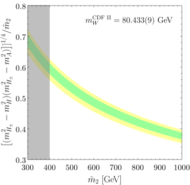
Refer to caption
(a)
Refer to caption
(b)
Figure 8: Parameter space where it is possible to explain the CDF II measurement of ๐ฆ๐–subscript๐ฆ๐–m_{W} via oblique ๐“๐“T parameter. In green(yellow) the experimental value at ๐Ÿโ€‹๐›”1๐›”1\sigma(๐Ÿโ€‹๐›”2๐›”2\sigma). In the grey shaded area the ๐ฏ/๐ฆ~๐Ÿ๐ฏsubscriptbold-~๐ฆ2v/\widetilde{m}_{2} expansion is not precise and can be affected by โ‰ณ๐“žโ€‹(๐Ÿ’๐ŸŽ%)greater-than-or-equivalent-toabsent๐“žpercent40\gtrsim\mathcal{O}(40\%) corrections.

It is interesting to notice that the explanation of ๐’Ž๐‘พsubscript๐’Ž๐‘พm_{W} fixes also the ordering of the mass hierarchy among the heavy scalars, leaving just two possibilities:

๐’Ž๐‘ฏยฑ๐Ÿ>๐’Ž๐‘ฏ๐Ÿ,๐’Ž๐‘จ๐Ÿ,๐’Ž๐‘ฏยฑ๐Ÿ<๐’Ž๐‘ฏ๐Ÿ,๐’Ž๐‘จ๐Ÿ.formulae-sequencesuperscriptsubscript๐’Žsubscript๐‘ฏplus-or-minus2superscriptsubscript๐’Ž๐‘ฏ2superscriptsubscript๐’Ž๐‘จ2superscriptsubscript๐’Žsubscript๐‘ฏplus-or-minus2superscriptsubscript๐’Ž๐‘ฏ2superscriptsubscript๐’Ž๐‘จ2m_{H_{\pm}}^{2}>m_{H}^{2},\leavevmode\nobreak\ m_{A}^{2}\,,\qquad\qquad\qquad m_{H_{\pm}}^{2}<m_{H}^{2},\leavevmode\nobreak\ m_{A}^{2}\,. (3.24)

On the other side, if the CDF II anomaly will lose evidence, this may be interpreted in the context of the ๐’๐Ÿsubscript๐’2Z_{2}-symmetric 2HDM as an indication of the (almost) degeneracy of the heavy scalar masses.

4 Conclusions

We have studied the predictions of the ๐’๐Ÿsubscript๐’2Z_{2} symmetric 2HD models near the decoupling limit, motivated by no discovery so far of any new scalar. After integrating out the heavy particles, the models can be formulated in terms of effective Lagrangians that depend on only three parameters: ๐ญ๐š๐งโก๐œท๐œท\tan\beta, the (approximately) common mass of the heavy scalars ๐’Ž~๐Ÿsubscriptbold-~๐’Ž2\widetilde{m}_{2}, and a complex coupling ๐€~๐Ÿ”subscriptbold-~๐€6\widetilde{\lambda}_{6} in the scalar potential. Due to the small number of free parameters, the effective models predict many correlations between observables, which are relevant both for analysing the present experimental constraints and the future discovery prospects.

The effective 2HD models are interesting theoretical laboratories for investigating the interplay of the flavour and collider constraints on the extensions of the SM, along the lines proposed in Refs. [49, 50]. The flavour ๐’๐Ÿsubscript๐’2Z_{2} symmetry eliminates the tree-level contributions to the FCNC and, therefore, new scalars with a relatively low mass scale may couple to the SM gauge bosons and fermions consistently with the constraints from the very high precision flavour data. In the effective approach, the predicted contributions to flavour-changing observables depend only on the value of ๐ญ๐š๐งโก๐œท๐œท\tan\beta (entering through Yukawa couplings) and on the degenerate heavy scalar masses ๐’Ž~๐Ÿsubscriptbold-~๐’Ž2\widetilde{m}_{2}. A fit to almost 60 observables gives the exclusions limits on ๐’Ž~๐Ÿsubscriptbold-~๐’Ž2\widetilde{m}_{2}, depending on type I-IV of the 2HDM and the value of ๐ญ๐š๐งโก๐œท๐œท\tan\beta: in particular, for the Type IV a lower bound on ๐’Ž~๐Ÿsubscriptbold-~๐’Ž2\widetilde{m}_{2} in the range ๐Ÿ‘๐ŸŽ๐ŸŽโˆ’๐Ÿ“๐ŸŽ๐ŸŽโ€‹GeV300500GeV300-500\ \text{GeV} is found; a similar limit applies in the Type-II scenario, but only for values of ๐ญ๐š๐งโก๐œท๐œท\tan\beta in the range ๐Ÿ๐ŸŽโˆ’๐Ÿ’๐ŸŽ204020-40, otherwise the bounds are weaker.

With these relatively weak bounds from flavour data, a complementary source of information on the effective Yukawa couplings and on the Lagrangian parameter comes from collider data on the Higgs production and decays. Strong correlations between different Yukawa couplings are predicted by the models. They have an impact on the results of the fit to the present data and determine the room left for deviations from the SM, important for future discovery prospects. The striking prediction of all four types of 2HD models is that the top quark Yukawa coupling is the least promising to show deviations from the SM value. The correlations among the effective Yukawa couplings are equally important for the bounds on the imaginary parts of the Yukawas inferred from the EDM bounds.

Another prediction following from the fits to flavour and Higgs data is for the expected range of the triple Higgs coupling: the deviations from the SM prediction, in the absence of hierarchies between ๐€~๐Ÿ”subscriptbold-~๐€6\widetilde{\lambda}_{6} and ๐€~๐Ÿ‘,๐Ÿ’,๐Ÿ“subscriptbold-~๐€345\widetilde{\lambda}_{3,4,5}, are tiny in the Type II and III models for any value of ๐ญ๐š๐งโก๐œท๐œท\tan\beta and in the Type IV for large ๐ญ๐š๐งโก๐œท๐œท\tan\beta; in the other cases the deviations may be sizeable and therefore testable in the future colliders.

Acknowledgements

The authors thanks Francisco Arco Garcรญa and Josรฉ Miguel No for useful discussions. A.d.G. and L.M. thanks the Institute of Theoretical Physics and the Faculty of Physics of the University of Warsaw for hospitality during the development of this project. S.P. thanks the Institute of Theoretical Physics of the Universidad Autรณnoma de Madrid for hospitality during the development of this project. A.d.G. and L.M. acknowledge partial financial support by the Spanish Research Agency (Agencia Estatal de Investigaciรณn) through the grant IFT Centro de Excelencia Severo Ochoa No CEX2020-001007-S and by the grant PID2019-108892RB-I00 funded by MCIN/AEI/ 10.13039/501100011033, by the European Unionโ€™s Horizon 2020 research and innovation programme under the Marie Skล‚odowska-Curie grant agreements No 860881-HIDDeN and 101086085-ASYMMETRY. The work of A.d.G. is supported by the European Unionโ€™s Horizon 2020 Marie Skล‚odowska-Curie grant agreement No 860881-HIDDeN. The research of S.P. has received partial financial support by the National Science Centre, Poland, grant DEC-2018/31/B/ST2/02283.

Appendix A From the ๐’๐Ÿsubscript๐’2Z_{2}-original basis to the Higgs basis

In this appendix, we define the scalar sector of the Lagrangian and its connection to the Higgs basis used in Sec. 2 following the notation of Ref. [88].

The scalar sector is composed of two identical complex scalar fields ๐šฝ๐’‚subscript๐šฝ๐’‚\Phi_{a}, with ๐’‚=๐Ÿ,๐Ÿ๐’‚12a=1,2, which are charged under ๐‘บโ€‹๐‘ผ๐‘ณโ€‹(๐Ÿ)ร—๐‘ผ๐’€โ€‹(๐Ÿ)๐‘บsubscript๐‘ผ๐‘ณ2subscript๐‘ผ๐’€1SU_{L}(2)\times U_{Y}(1) and with hypercharge, ๐’€๐šฝ๐’‚=๐Ÿ/๐Ÿsubscript๐’€subscript๐šฝ๐’‚12Y_{\Phi_{a}}=1/2. The Lagrangian reads

๐“›=(๐‘ซ๐โ€‹๐šฝ๐’‚)โ€ โ€‹(๐‘ซ๐โ€‹๐šฝ๐’‚)+๐‘ฝโ€‹(๐šฝ๐Ÿ,๐šฝ๐Ÿ),๐“›superscriptsubscript๐‘ซ๐subscript๐šฝ๐’‚bold-โ€ superscript๐‘ซ๐subscript๐šฝ๐’‚๐‘ฝsubscript๐šฝ1subscript๐šฝ2\mathscr{L}=(D_{\mu}\Phi_{a})^{\dagger}(D^{\mu}\Phi_{a})+V(\Phi_{1},\Phi_{2})\,, (A.1)

where the most general renormalizable potential for the two doublets reads

๐‘ฝโ€‹(๐šฝ๐Ÿ,๐šฝ๐Ÿ)=๐‘ฝsubscript๐šฝ1subscript๐šฝ2absent\displaystyle V(\Phi_{1},\Phi_{2})= โˆ’๐’Ž๐Ÿ๐Ÿโ€‹(๐šฝ๐Ÿโ€ โ€‹๐šฝ๐Ÿ)โˆ’๐’Ž๐Ÿ๐Ÿโ€‹(๐šฝ๐Ÿโ€ โ€‹๐šฝ๐Ÿ)โˆ’[๐’Ž๐Ÿ๐Ÿ๐Ÿโ€‹(๐šฝ๐Ÿโ€ โ€‹๐šฝ๐Ÿ)+h.c.]superscriptsubscript๐’Ž12subscriptsuperscript๐šฝbold-โ€ 1subscript๐šฝ1superscriptsubscript๐’Ž22subscriptsuperscript๐šฝbold-โ€ 2subscript๐šฝ2delimited-[]superscriptsubscript๐’Ž122subscriptsuperscript๐šฝbold-โ€ 1subscript๐šฝ2h.c.\displaystyle-m_{1}^{2}(\Phi^{\dagger}_{1}\Phi_{1})-m_{2}^{2}(\Phi^{\dagger}_{2}\Phi_{2})-\left[m_{12}^{2}(\Phi^{\dagger}_{1}\Phi_{2})+\text{h.c.}\right]
+๐€๐Ÿโ€‹(๐šฝ๐Ÿโ€ โ€‹๐šฝ๐Ÿ)๐Ÿ+๐€๐Ÿโ€‹(๐šฝ๐Ÿโ€ โ€‹๐šฝ๐Ÿ)๐Ÿ+๐€๐Ÿ‘โ€‹(๐šฝ๐Ÿโ€ โ€‹๐šฝ๐Ÿ)โ€‹(๐šฝ๐Ÿโ€ โ€‹๐šฝ๐Ÿ)+๐€๐Ÿ’โ€‹(๐šฝ๐Ÿโ€ โ€‹๐šฝ๐Ÿ)โ€‹(๐šฝ๐Ÿโ€ โ€‹๐šฝ๐Ÿ)subscript๐€1superscriptsubscriptsuperscript๐šฝbold-โ€ 1subscript๐šฝ12subscript๐€2superscriptsubscriptsuperscript๐šฝbold-โ€ 2subscript๐šฝ22subscript๐€3subscriptsuperscript๐šฝbold-โ€ 1subscript๐šฝ1subscriptsuperscript๐šฝbold-โ€ 2subscript๐šฝ2subscript๐€4subscriptsuperscript๐šฝbold-โ€ 1subscript๐šฝ2subscriptsuperscript๐šฝbold-โ€ 2subscript๐šฝ1\displaystyle+\lambda_{1}(\Phi^{\dagger}_{1}\Phi_{1})^{2}+\lambda_{2}(\Phi^{\dagger}_{2}\Phi_{2})^{2}+\lambda_{3}(\Phi^{\dagger}_{1}\Phi_{1})(\Phi^{\dagger}_{2}\Phi_{2})+\lambda_{4}(\Phi^{\dagger}_{1}\Phi_{2})(\Phi^{\dagger}_{2}\Phi_{1})
+[๐€๐Ÿ“โ€‹(๐šฝ๐Ÿโ€ โ€‹๐šฝ๐Ÿ)๐Ÿ+๐€๐Ÿ”โ€‹(๐šฝ๐Ÿโ€ โ€‹๐šฝ๐Ÿ)โ€‹(๐šฝ๐Ÿโ€ โ€‹๐šฝ๐Ÿ)+๐€๐Ÿ•โ€‹(๐šฝ๐Ÿโ€ โ€‹๐šฝ๐Ÿ)โ€‹(๐šฝ๐Ÿโ€ โ€‹๐šฝ๐Ÿ)+h.c.].delimited-[]subscript๐€5superscriptsubscriptsuperscript๐šฝbold-โ€ 1subscript๐šฝ22subscript๐€6subscriptsuperscript๐šฝbold-โ€ 1subscript๐šฝ1subscriptsuperscript๐šฝbold-โ€ 1subscript๐šฝ2subscript๐€7subscriptsuperscript๐šฝbold-โ€ 2subscript๐šฝ2subscriptsuperscript๐šฝbold-โ€ 1subscript๐šฝ2h.c.\displaystyle+\left[\lambda_{5}(\Phi^{\dagger}_{1}\Phi_{2})^{2}+\lambda_{6}(\Phi^{\dagger}_{1}\Phi_{1})(\Phi^{\dagger}_{1}\Phi_{2})+\lambda_{7}(\Phi^{\dagger}_{2}\Phi_{2})(\Phi^{\dagger}_{1}\Phi_{2})+\text{h.c.}\right]\,.

The parameters ๐’Ž๐Ÿ๐Ÿ,๐’Ž๐Ÿ๐Ÿ,๐€๐Ÿ,๐€๐Ÿ,๐€๐Ÿ‘superscriptsubscript๐’Ž12superscriptsubscript๐’Ž22subscript๐€1subscript๐€2subscript๐€3m_{1}^{2},m_{2}^{2},\lambda_{1},\lambda_{2},\lambda_{3} and ๐€๐Ÿ’subscript๐€4\lambda_{4} are real while ๐’Ž๐Ÿ๐Ÿ๐Ÿ,๐€๐Ÿ“,๐€๐Ÿ”superscriptsubscript๐’Ž122subscript๐€5subscript๐€6m_{12}^{2},\lambda_{5},\lambda_{6} and ๐€๐Ÿ•subscript๐€7\lambda_{7} are in general complex.

In the ๐šฝ๐šฝ\Phi-basis, both Higgs doublets get a vev. Without loss of generality, one can write

โŸจ๐šฝ๐Ÿโ€ โ€‹๐šฝ๐ŸโŸฉ=๐’—๐Ÿ๐Ÿ๐Ÿ,โŸจ๐šฝ๐Ÿโ€ โ€‹๐šฝ๐ŸโŸฉ=๐’—๐Ÿ๐Ÿ๐Ÿ,๐ƒโ‰ก๐š๐ซ๐ โกโŸจ๐šฝ๐Ÿโ€ โ€‹๐šฝ๐ŸโŸฉformulae-sequencedelimited-โŸจโŸฉsuperscriptsubscript๐šฝ1bold-โ€ subscript๐šฝ1superscriptsubscript๐’—122formulae-sequencedelimited-โŸจโŸฉsuperscriptsubscript๐šฝ2bold-โ€ subscript๐šฝ2superscriptsubscript๐’—222๐ƒsuperscriptsubscript๐šฝ1bold-โ€ subscript๐šฝ2\left<\Phi_{1}^{\dagger}\Phi_{1}\right>=\dfrac{v_{1}^{2}}{2}\,,\qquad\left<\Phi_{2}^{\dagger}\Phi_{2}\right>=\dfrac{v_{2}^{2}}{2}\,,\qquad\xi\equiv\arg\left<\Phi_{1}^{\dagger}\Phi_{2}\right> (A.2)

where, ๐’—๐Ÿ,๐’—๐Ÿ,๐ƒsubscript๐’—1subscript๐’—2๐ƒv_{1},v_{2},\xi are real, ๐’—๐Ÿ=๐’—๐Ÿ๐Ÿ+๐’—๐Ÿ๐Ÿ=(๐Ÿ๐Ÿ’๐Ÿ”โ€‹GeV)๐Ÿsuperscript๐’—2superscriptsubscript๐’—12superscriptsubscript๐’—22superscript246GeV2v^{2}=v_{1}^{2}+v_{2}^{2}=(246\,\text{GeV})^{2} and

๐ญ๐š๐งโก๐œทโ‰ก๐’—๐Ÿ๐’—๐Ÿ.๐œทsubscript๐’—2subscript๐’—1\tan\beta\equiv\frac{v_{2}}{v_{1}}\,. (A.3)

Under the โ„ค๐Ÿsubscriptโ„ค2\mathbb{Z}_{2} symmetry the doublets transform differently as

๐šฝ๐Ÿโ†’+๐šฝ๐Ÿand๐šฝ๐Ÿโ†’โˆ’๐šฝ๐Ÿformulae-sequencebold-โ†’subscript๐šฝ1subscript๐šฝ1andbold-โ†’subscript๐šฝ2subscript๐šฝ2\Phi_{1}\to+\Phi_{1}\qquad\text{and}\qquad\Phi_{2}\to-\Phi_{2} (A.4)

which in turn enforces the condition

๐€๐Ÿ”=๐€๐Ÿ•=๐ŸŽsubscript๐€6subscript๐€70\lambda_{6}=\lambda_{7}=0 (A.5)

We allow the discrete symmetry to be softly broken in the potential by ๐’Ž๐Ÿ๐Ÿ๐Ÿsubscriptsuperscript๐’Ž212m^{2}_{12}.

The Higgs basis is defined by the condition that only one doublet admits a vev, i.e.

โŸจ๐‘ฏ๐Ÿโ€ โ€‹๐‘ฏ๐ŸโŸฉ=๐’—๐Ÿ๐Ÿ,โŸจ๐‘ฏ๐Ÿโ€ โ€‹๐‘ฏ๐ŸโŸฉ=๐ŸŽ.formulae-sequencedelimited-โŸจโŸฉsuperscriptsubscript๐‘ฏ1bold-โ€ subscript๐‘ฏ1superscript๐’—22delimited-โŸจโŸฉsuperscriptsubscript๐‘ฏ2bold-โ€ subscript๐‘ฏ20\left<H_{1}^{\dagger}H_{1}\right>=\dfrac{v^{2}}{2}\,,\qquad\left<H_{2}^{\dagger}H_{2}\right>=0\,. (A.6)

It can be reached by a rotation of the doublets

(๐’†โˆ’๐’Šโ€‹๐ƒ/๐Ÿโ€‹๐‘ฏ๐Ÿ๐‘ฏ๐Ÿ)=(๐’„๐œท๐’”๐œทโ€‹๐’†โˆ’๐’Šโ€‹๐ƒโˆ’๐’”๐œทโ€‹๐’†๐’Šโ€‹๐ƒ๐’„๐œท)โ€‹(๐šฝ๐Ÿ๐šฝ๐Ÿ)matrixsuperscript๐’†๐’Š๐ƒ2subscript๐‘ฏ1subscript๐‘ฏ2matrixsubscript๐’„๐œทsubscript๐’”๐œทsuperscript๐’†๐’Š๐ƒsubscript๐’”๐œทsuperscript๐’†๐’Š๐ƒsubscript๐’„๐œทmatrixsubscript๐šฝ1subscript๐šฝ2\begin{pmatrix}e^{-i\xi/2}H_{1}\\ H_{2}\\ \end{pmatrix}=\begin{pmatrix}c_{\beta}&s_{\beta}e^{-i\xi}\\ -s_{\beta}e^{i\xi}&c_{\beta}\\ \end{pmatrix}\begin{pmatrix}\Phi_{1}\\ \Phi_{2}\\ \end{pmatrix} (A.7)

As the โ„ค๐Ÿsubscriptโ„ค2\mathbb{Z}_{2}-symmetry is not defined in this basis, ๐€๐Ÿ”subscript๐€6\lambda_{6}- and ๐€๐Ÿ•subscript๐€7\lambda_{7}-like terms are again developed. The potential reads

๐‘ฝโ€‹(๐‘ฏ๐Ÿ,๐‘ฏ๐Ÿ)=๐‘ฝsubscript๐‘ฏ1subscript๐‘ฏ2absent\displaystyle V(H_{1},H_{2})=\, ๐’Ž~๐Ÿ๐Ÿโ€‹๐‘ฏ๐Ÿโ€ โ€‹๐‘ฏ๐Ÿ+๐’Ž~๐Ÿ๐Ÿโ€‹๐‘ฏ๐Ÿโ€ โ€‹๐‘ฏ๐Ÿโˆ’(๐’Ž~๐Ÿ๐Ÿ๐Ÿโ€‹๐‘ฏ๐Ÿโ€ โ€‹๐‘ฏ๐Ÿ+h.c.)+๐Ÿ๐Ÿโ€‹๐€~๐Ÿโ€‹(๐‘ฏ๐Ÿโ€ โ€‹๐‘ฏ๐Ÿ)๐Ÿ+superscriptsubscriptbold-~๐’Ž12superscriptsubscript๐‘ฏ1bold-โ€ subscript๐‘ฏ1superscriptsubscriptbold-~๐’Ž22superscriptsubscript๐‘ฏ2bold-โ€ subscript๐‘ฏ2superscriptsubscriptbold-~๐’Ž122superscriptsubscript๐‘ฏ1bold-โ€ subscript๐‘ฏ2h.c.limit-from12subscriptbold-~๐€1superscriptsuperscriptsubscript๐‘ฏ1bold-โ€ subscript๐‘ฏ12\displaystyle\widetilde{m}_{1}^{2}H_{1}^{\dagger}H_{1}+\widetilde{m}_{2}^{2}H_{2}^{\dagger}H_{2}-\left(\widetilde{m}_{12}^{2}H_{1}^{\dagger}H_{2}+\text{h.c.}\right)+\dfrac{1}{2}\widetilde{\lambda}_{1}\left(H_{1}^{\dagger}H_{1}\right)^{2}+
+๐Ÿ๐Ÿโ€‹๐€~๐Ÿโ€‹(๐‘ฏ๐Ÿโ€ โ€‹๐‘ฏ๐Ÿ)๐Ÿ+๐€~๐Ÿ‘โ€‹(๐‘ฏ๐Ÿโ€ โ€‹๐‘ฏ๐Ÿ)โ€‹(๐‘ฏ๐Ÿโ€ โ€‹๐‘ฏ๐Ÿ)+๐€~๐Ÿ’โ€‹(๐‘ฏ๐Ÿโ€ โ€‹๐‘ฏ๐Ÿ)โ€‹(๐‘ฏ๐Ÿโ€ โ€‹๐‘ฏ๐Ÿ)+12subscriptbold-~๐€2superscriptsuperscriptsubscript๐‘ฏ2bold-โ€ subscript๐‘ฏ22subscriptbold-~๐€3superscriptsubscript๐‘ฏ1bold-โ€ subscript๐‘ฏ1superscriptsubscript๐‘ฏ2bold-โ€ subscript๐‘ฏ2limit-fromsubscriptbold-~๐€4superscriptsubscript๐‘ฏ1bold-โ€ subscript๐‘ฏ2superscriptsubscript๐‘ฏ2bold-โ€ subscript๐‘ฏ1\displaystyle+\dfrac{1}{2}\widetilde{\lambda}_{2}\left(H_{2}^{\dagger}H_{2}\right)^{2}+\widetilde{\lambda}_{3}\left(H_{1}^{\dagger}H_{1}\right)\left(H_{2}^{\dagger}H_{2}\right)+\widetilde{\lambda}_{4}\left(H_{1}^{\dagger}H_{2}\right)\left(H_{2}^{\dagger}H_{1}\right)+ (A.8)
+[๐Ÿ๐Ÿโ€‹๐€~๐Ÿ“โ€‹(๐‘ฏ๐Ÿโ€ โ€‹๐‘ฏ๐Ÿ)๐Ÿ+๐€~๐Ÿ”โ€‹(๐‘ฏ๐Ÿโ€ โ€‹๐‘ฏ๐Ÿ)โ€‹(๐‘ฏ๐Ÿโ€ โ€‹๐‘ฏ๐Ÿ)+๐€~๐Ÿ•โ€‹(๐‘ฏ๐Ÿโ€ โ€‹๐‘ฏ๐Ÿ)โ€‹(๐‘ฏ๐Ÿโ€ โ€‹๐‘ฏ๐Ÿ)+h.c.].delimited-[]12subscriptbold-~๐€5superscriptsuperscriptsubscript๐‘ฏ1bold-โ€ subscript๐‘ฏ22subscriptbold-~๐€6superscriptsubscript๐‘ฏ1bold-โ€ subscript๐‘ฏ1superscriptsubscript๐‘ฏ1bold-โ€ subscript๐‘ฏ2subscriptbold-~๐€7superscriptsubscript๐‘ฏ2bold-โ€ subscript๐‘ฏ2superscriptsubscript๐‘ฏ1bold-โ€ subscript๐‘ฏ2h.c.\displaystyle+\left[\dfrac{1}{2}\widetilde{\lambda}_{5}\left(H_{1}^{\dagger}H_{2}\right)^{2}+\widetilde{\lambda}_{6}\left(H_{1}^{\dagger}H_{1}\right)\left(H_{1}^{\dagger}H_{2}\right)+\widetilde{\lambda}_{7}\left(H_{2}^{\dagger}H_{2}\right)\left(H_{1}^{\dagger}H_{2}\right)+\text{h.c.}\right]\,. (A.9)

The tilded parameters are defined in terms of the original ones via

๐’Ž~๐Ÿ๐Ÿsuperscriptsubscriptbold-~๐’Ž12\displaystyle\widetilde{m}_{1}^{2} =๐’Ž๐Ÿ๐Ÿโ€‹๐’„๐œท๐Ÿ+๐’Ž๐Ÿ๐Ÿโ€‹๐’”๐œท๐Ÿ+๐’”๐Ÿโ€‹๐œทโ€‹Reโ€‹(๐’Ž๐Ÿ๐Ÿ๐Ÿโ€‹๐’†๐’Šโ€‹๐ƒ),absentsuperscriptsubscript๐’Ž12superscriptsubscript๐’„๐œท2superscriptsubscript๐’Ž22superscriptsubscript๐’”๐œท2subscript๐’”2๐œทResuperscriptsubscript๐’Ž122superscript๐’†๐’Š๐ƒ\displaystyle=m_{1}^{2}c_{\beta}^{2}+m_{2}^{2}s_{\beta}^{2}+s_{2\beta}{\texttt{Re}}(m_{12}^{2}e^{i\xi})\,, (A.10)
๐’Ž~๐Ÿ๐Ÿsuperscriptsubscriptbold-~๐’Ž22\displaystyle\widetilde{m}_{2}^{2} =๐’Ž๐Ÿ๐Ÿโ€‹๐’”๐œท๐Ÿ+๐’Ž๐Ÿ๐Ÿโ€‹๐’„๐œท๐Ÿโˆ’๐’”๐Ÿโ€‹๐œทโ€‹Reโ€‹(๐’Ž๐Ÿ๐Ÿ๐Ÿโ€‹๐’†๐’Šโ€‹๐ƒ),absentsuperscriptsubscript๐’Ž12superscriptsubscript๐’”๐œท2superscriptsubscript๐’Ž22superscriptsubscript๐’„๐œท2subscript๐’”2๐œทResuperscriptsubscript๐’Ž122superscript๐’†๐’Š๐ƒ\displaystyle=m_{1}^{2}s_{\beta}^{2}+m_{2}^{2}c_{\beta}^{2}-s_{2\beta}{\texttt{Re}}(m_{12}^{2}e^{i\xi})\,,
๐’Ž~๐Ÿ๐Ÿ๐Ÿโ€‹๐’†๐’Šโ€‹๐ƒ/๐Ÿsuperscriptsubscriptbold-~๐’Ž122superscript๐’†๐’Š๐ƒ2\displaystyle\widetilde{m}_{12}^{2}e^{i\xi/2} =(๐’Ž๐Ÿ๐Ÿโˆ’๐’Ž๐Ÿ๐Ÿ)โ€‹๐’„๐œทโ€‹๐’”๐œท+Reโ€‹(๐’Ž๐Ÿ๐Ÿ๐Ÿโ€‹๐’†๐’Šโ€‹๐ƒ)โ€‹๐’„๐Ÿโ€‹๐œท+๐’Šโ€‹Imโ€‹(๐’Ž๐Ÿ๐Ÿ๐Ÿโ€‹๐’†๐’Šโ€‹๐ƒ),absentsuperscriptsubscript๐’Ž22superscriptsubscript๐’Ž12subscript๐’„๐œทsubscript๐’”๐œทResuperscriptsubscript๐’Ž122superscript๐’†๐’Š๐ƒsubscript๐’„2๐œท๐’ŠImsuperscriptsubscript๐’Ž122superscript๐’†๐’Š๐ƒ\displaystyle=(m_{2}^{2}-m_{1}^{2})c_{\beta}s_{\beta}+{\texttt{Re}}(m_{12}^{2}e^{i\xi})c_{2\beta}+i{\texttt{Im}}(m_{12}^{2}e^{i\xi})\,,

and

๐€~๐Ÿsubscriptbold-~๐€1\displaystyle\widetilde{\lambda}_{1} =๐€๐Ÿโ€‹๐’„๐œท๐Ÿ’+๐€๐Ÿโ€‹๐’”๐œท๐Ÿ’+๐€๐Ÿ‘๐Ÿ’๐Ÿ“โ€‹๐’„๐œท๐Ÿโ€‹๐’”๐œท๐Ÿ,absentsubscript๐€1superscriptsubscript๐’„๐œท4subscript๐€2superscriptsubscript๐’”๐œท4subscript๐€345subscriptsuperscript๐’„2๐œทsubscriptsuperscript๐’”2๐œท\displaystyle=\lambda_{1}c_{\beta}^{4}+\lambda_{2}s_{\beta}^{4}+\lambda_{345}c^{2}_{\beta}s^{2}_{\beta}\,, (A.11)
๐€~๐Ÿsubscriptbold-~๐€2\displaystyle\widetilde{\lambda}_{2} =๐€๐Ÿโ€‹๐’”๐œท๐Ÿ’+๐€๐Ÿโ€‹๐’„๐œท๐Ÿ’+๐€๐Ÿ‘๐Ÿ’๐Ÿ“โ€‹๐’„๐œท๐Ÿโ€‹๐’”๐œท๐Ÿ,absentsubscript๐€1superscriptsubscript๐’”๐œท4subscript๐€2superscriptsubscript๐’„๐œท4subscript๐€345subscriptsuperscript๐’„2๐œทsubscriptsuperscript๐’”2๐œท\displaystyle=\lambda_{1}s_{\beta}^{4}+\lambda_{2}c_{\beta}^{4}+\lambda_{345}c^{2}_{\beta}s^{2}_{\beta}\,,
๐€~๐Ÿ‘subscriptbold-~๐€3\displaystyle\widetilde{\lambda}_{3} =๐€๐Ÿ‘+(๐€๐Ÿ+๐€๐Ÿโˆ’๐€๐Ÿ‘๐Ÿ’๐Ÿ“)โ€‹๐’”๐Ÿโ€‹๐œท๐Ÿ๐Ÿ’,absentsubscript๐€3subscript๐€1subscript๐€2subscript๐€345subscriptsuperscript๐’”22๐œท4\displaystyle=\lambda_{3}+(\lambda_{1}+\lambda_{2}-\lambda_{345})\frac{s^{2}_{2\beta}}{4}\,,
๐€~๐Ÿ’subscriptbold-~๐€4\displaystyle\widetilde{\lambda}_{4} =๐€๐Ÿ’+(๐€๐Ÿ+๐€๐Ÿโˆ’๐€๐Ÿ‘๐Ÿ’๐Ÿ“)โ€‹๐’”๐Ÿโ€‹๐œท๐Ÿ๐Ÿ’,absentsubscript๐€4subscript๐€1subscript๐€2subscript๐€345subscriptsuperscript๐’”22๐œท4\displaystyle=\lambda_{4}+(\lambda_{1}+\lambda_{2}-\lambda_{345})\frac{s^{2}_{2\beta}}{4}\,,
๐€~๐Ÿ“โ€‹๐’†๐’Šโ€‹๐ƒ/๐Ÿsubscriptbold-~๐€5superscript๐’†๐’Š๐ƒ2\displaystyle\widetilde{\lambda}_{5}e^{i\xi/2} =๐’”๐Ÿโ€‹๐œท๐Ÿ๐Ÿ’โ€‹(๐€๐Ÿ+๐€๐Ÿโˆ’๐€๐Ÿ‘๐Ÿ’๐Ÿ“)+Reโ€‹(๐€๐Ÿ“โ€‹๐’†๐Ÿโ€‹๐’Šโ€‹๐ƒ)+๐’Šโ€‹๐’„๐Ÿโ€‹๐œทโ€‹Imโ€‹(๐€๐Ÿ“โ€‹๐’†๐Ÿโ€‹๐’Šโ€‹๐ƒ),absentsubscriptsuperscript๐’”22๐œท4subscript๐€1subscript๐€2subscript๐€345Resubscript๐€5superscript๐’†2๐’Š๐ƒ๐’Šsubscript๐’„2๐œทImsubscript๐€5superscript๐’†2๐’Š๐ƒ\displaystyle=\dfrac{s^{2}_{2\beta}}{4}(\lambda_{1}+\lambda_{2}-\lambda_{345})+{\texttt{Re}}(\lambda_{5}e^{2i\xi})+ic_{2\beta}{\texttt{Im}}(\lambda_{5}e^{2i\xi})\,,
๐€~๐Ÿ”โ€‹๐’†๐’Šโ€‹๐ƒ/๐Ÿsubscriptbold-~๐€6superscript๐’†๐’Š๐ƒ2\displaystyle\widetilde{\lambda}_{6}e^{i\xi/2} =โˆ’๐’”๐Ÿโ€‹๐œท๐Ÿโ€‹(๐€๐Ÿโ€‹๐’„๐œท๐Ÿโˆ’๐€๐Ÿโ€‹๐’”๐œท๐Ÿโˆ’๐€๐Ÿ‘๐Ÿ’๐Ÿ“โ€‹๐’„๐Ÿโ€‹๐œทโˆ’๐’Šโ€‹Imโ€‹(๐€๐Ÿ“โ€‹๐’†๐Ÿโ€‹๐’Šโ€‹๐ƒ)),absentsubscript๐’”2๐œท2subscript๐€1superscriptsubscript๐’„๐œท2subscript๐€2superscriptsubscript๐’”๐œท2subscript๐€345subscript๐’„2๐œท๐’ŠImsubscript๐€5superscript๐’†2๐’Š๐ƒ\displaystyle=-\frac{s_{2\beta}}{2}(\lambda_{1}c_{\beta}^{2}-\lambda_{2}s_{\beta}^{2}-\lambda_{345}c_{2\beta}-i{\texttt{Im}}(\lambda_{5}e^{2i\xi}))\,,
๐€~๐Ÿ•โ€‹๐’†๐’Šโ€‹๐ƒ/๐Ÿsubscriptbold-~๐€7superscript๐’†๐’Š๐ƒ2\displaystyle\widetilde{\lambda}_{7}e^{i\xi/2} =โˆ’๐’”๐Ÿโ€‹๐œท๐Ÿโ€‹(๐€๐Ÿโ€‹๐’”๐œท๐Ÿโˆ’๐€๐Ÿโ€‹๐’„๐œท๐Ÿ+๐€๐Ÿ‘๐Ÿ’๐Ÿ“โ€‹๐’„๐Ÿโ€‹๐œท+๐’Šโ€‹Imโ€‹(๐€๐Ÿ“โ€‹๐’†๐Ÿโ€‹๐’Šโ€‹๐ƒ))absentsubscript๐’”2๐œท2subscript๐€1superscriptsubscript๐’”๐œท2subscript๐€2superscriptsubscript๐’„๐œท2subscript๐€345subscript๐’„2๐œท๐’ŠImsubscript๐€5superscript๐’†2๐’Š๐ƒ\displaystyle=-\frac{s_{2\beta}}{2}(\lambda_{1}s_{\beta}^{2}-\lambda_{2}c_{\beta}^{2}+\lambda_{345}c_{2\beta}+i{\texttt{Im}}(\lambda_{5}e^{2i\xi}))

where ๐€๐Ÿ‘๐Ÿ’๐Ÿ“=๐€๐Ÿ‘+๐€๐Ÿ’+Reโ€‹(๐€๐Ÿ“โ€‹๐’†๐Ÿโ€‹๐’Šโ€‹๐ƒ)subscript๐€345subscript๐€3subscript๐€4Resubscript๐€5superscript๐’†2๐’Š๐ƒ\lambda_{345}=\lambda_{3}+\lambda_{4}+{\texttt{Re}}(\lambda_{5}e^{2i\xi}).

References

  • [1] ATLAS Collaboration, G. Aad et. al., Observation of a new particle in the search for the Standard Model Higgs boson with the ATLAS detector at the LHC, Phys. Lett. B 716 (2012) 1โ€“29, [arXiv:1207.7214].
  • [2] CMS Collaboration, S. Chatrchyan et. al., Observation of a New Boson at a Mass of 125 GeV with the CMS Experiment at the LHC, Phys. Lett. B 716 (2012) 30โ€“61, [arXiv:1207.7235].
  • [3] W. Buchmuller and D. Wyler, Effective Lagrangian Analysis of New Interactions and Flavor Conservation, Nucl. Phys. B 268 (1986) 621โ€“653.
  • [4] B. Grzadkowski, M. Iskrzynski, M. Misiak, and J. Rosiek, Dimension-Six Terms in the Standard Model Lagrangian, JHEP 10 (2010) 085, [arXiv:1008.4884].
  • [5] F. Feruglio, The Chiral approach to the electroweak interactions, Int. J. Mod. Phys. A 8 (1993) 4937โ€“4972, [hep-ph/9301281].
  • [6] B. Grinstein and M. Trott, A Higgs-Higgs bound state due to new physics at a TeV, Phys. Rev. D 76 (2007) 073002, [arXiv:0704.1505].
  • [7] R. Contino, C. Grojean, M. Moretti, F. Piccinini, and R. Rattazzi, Strong Double Higgs Production at the LHC, JHEP 05 (2010) 089, [arXiv:1002.1011].
  • [8] R. Alonso, M. B. Gavela, L. Merlo, S. Rigolin, and J. Yepes, The Effective Chiral Lagrangian for a Light Dynamical โ€Higgs Particleโ€, Phys. Lett. B 722 (2013) 330โ€“335, [arXiv:1212.3305]. [Erratum: Phys.Lett.B 726, 926 (2013)].
  • [9] R. Alonso, M. B. Gavela, L. Merlo, S. Rigolin, and J. Yepes, Flavor with a light dynamical โ€Higgs particleโ€, Phys. Rev. D 87 (2013), no. 5 055019, [arXiv:1212.3307].
  • [10] I. Brivio, T. Corbett, O. J. P. ร‰boli, M. B. Gavela, J. Gonzalez-Fraile, M. C. Gonzalez-Garcia, L. Merlo, and S. Rigolin, Disentangling a dynamical Higgs, JHEP 03 (2014) 024, [arXiv:1311.1823].
  • [11] M. B. Gavela, J. Gonzalez-Fraile, M. C. Gonzalez-Garcia, L. Merlo, S. Rigolin, and J. Yepes, CP violation with a dynamical Higgs, JHEP 10 (2014) 044, [arXiv:1406.6367].
  • [12] G. Buchalla, O. Catร , and C. Krause, Complete Electroweak Chiral Lagrangian with a Light Higgs at NLO, Nucl. Phys. B 880 (2014) 552โ€“573, [arXiv:1307.5017]. [Erratum: Nucl.Phys.B 913, 475โ€“478 (2016)].
  • [13] I. Brivio, O. J. P. ร‰boli, M. B. Gavela, M. C. Gonzalez-Garcia, L. Merlo, and S. Rigolin, Higgs ultraviolet softening, JHEP 12 (2014) 004, [arXiv:1405.5412].
  • [14] P. Kozรณw, L. Merlo, S. Pokorski, and M. Szleper, Same-sign WW Scattering in the HEFT: Discoverability vs. EFT Validity, JHEP 07 (2019) 021, [arXiv:1905.03354].
  • [15] R. Alonso, E. E. Jenkins, A. V. Manohar, and M. Trott, Renormalization Group Evolution of the Standard Model Dimension Six Operators III: Gauge Coupling Dependence and Phenomenology, JHEP 04 (2014) 159, [arXiv:1312.2014].
  • [16] O. J. P. Eboli, M. C. Gonzalez-Garcia, and M. Martines, Electroweak Higgs effective field theory after LHC run 2, Phys. Rev. D 105 (2022), no. 5 053003, [arXiv:2112.11468].
  • [17] CDF Collaboration, T. Aaltonen et. al., High-precision measurement of the ๐–๐–W boson mass with the CDF II detector, Science 376 (2022), no. 6589 170โ€“176.
  • [18] ATLAS Collaboration, Improved W boson Mass Measurement using 7 TeV Proton-Proton Collisions with the ATLAS Detector, tech. rep., CERN, Geneva, 2023. ATLAS-CONF-2023-004.
  • [19] M. Blennow, P. Coloma, E. Fernรกndez-Martรญnez, and M. Gonzรกlez-Lรณpez, Right-handed neutrinos and the CDF II anomaly, Phys. Rev. D 106 (2022), no. 7 073005, [arXiv:2204.04559].
  • [20] F. Arias-Aragรณn, E. Fernรกndez-Martรญnez, M. Gonzรกlez-Lรณpez, and L. Merlo, Dynamical Minimal Flavour Violating inverse seesaw, JHEP 09 (2022) 210, [arXiv:2204.04672].
  • [21] A. de Giorgi, L. Merlo, and S. Pokorski, The Low-Scale Seesaw Solution to the ๐Œ๐–subscript๐Œ๐–M_{W} and (๐ โˆ’๐Ÿ)๐›subscript๐ 2๐›(g-2)_{\mu} Anomalies, arXiv:2211.03797.
  • [22] K. Sakurai, F. Takahashi, and W. Yin, Singlet extensions and W boson mass in light of the CDF II result, Phys. Lett. B 833 (2022) 137324, [arXiv:2204.04770].
  • [23] A. Paul and M. Valli, Violation of custodial symmetry from W-boson mass measurements, Phys. Rev. D 106 (2022), no. 1 013008, [arXiv:2204.05267].
  • [24] BaBar Collaboration, J. P. Lees et. al., Evidence for an excess of ๐ยฏโ†’๐ƒ(โˆ—)โ€‹๐›•โˆ’โ€‹๐›Žยฏ๐›•bold-โ†’bold-ยฏ๐superscript๐ƒsuperscript๐›•subscriptbold-ยฏ๐›Ž๐›•\bar{B}\to D^{(*)}\tau^{-}\bar{\nu}_{\tau} decays, Phys. Rev. Lett. 109 (2012) 101802, [arXiv:1205.5442].
  • [25] BaBar Collaboration, J. P. Lees et. al., Measurement of an Excess of ๐ยฏโ†’๐ƒ(โˆ—)โ€‹๐›•โˆ’โ€‹๐›Žยฏ๐›•bold-โ†’bold-ยฏ๐superscript๐ƒsuperscript๐›•subscriptbold-ยฏ๐›Ž๐›•\bar{B}\to D^{(*)}\tau^{-}\bar{\nu}_{\tau} Decays and Implications for Charged Higgs Bosons, Phys. Rev. D 88 (2013), no. 7 072012, [arXiv:1303.0571].
  • [26] Belle Collaboration, A. Matyja et. al., Observation of B0 โ€”>> D*- tau+ nu(tau) decay at Belle, Phys. Rev. Lett. 99 (2007) 191807, [arXiv:0706.4429].
  • [27] Belle Collaboration, I. Adachi et. al., Measurement of B โ€”>> D(*) tau nu using full reconstruction tags, in 24th International Symposium on Lepton-Photon Interactions at High Energy (LP09), 10, 2009. arXiv:0910.4301.
  • [28] Belle Collaboration, A. Bozek et. al., Observation of ๐+โ†’๐ƒยฏโˆ—โ€‹๐ŸŽโ€‹๐›•+โ€‹๐›Ž๐›•bold-โ†’superscript๐superscriptbold-ยฏ๐ƒ0superscript๐›•subscript๐›Ž๐›•B^{+}\to\bar{D}^{*}0\tau^{+}\nu_{\tau} and Evidence for ๐+โ†’๐ƒยฏ๐ŸŽโ€‹๐›•+โ€‹๐›Ž๐›•bold-โ†’superscript๐superscriptbold-ยฏ๐ƒ0superscript๐›•subscript๐›Ž๐›•B^{+}\to\bar{D}^{0}\tau^{+}\nu_{\tau} at Belle, Phys. Rev. D 82 (2010) 072005, [arXiv:1005.2302].
  • [29] Y. Sakaki, M. Tanaka, A. Tayduganov, and R. Watanabe, Testing leptoquark models in ๐ยฏโ†’๐ƒ(โˆ—)โ€‹๐›•โ€‹๐›Žยฏbold-โ†’bold-ยฏ๐superscript๐ƒ๐›•bold-ยฏ๐›Ž\bar{B}\to D^{(*)}\tau\bar{\nu}, Phys. Rev. D 88 (2013), no. 9 094012, [arXiv:1309.0301].
  • [30] LHCb Collaboration, R. Puthumanaillam, Measurement of ๐‘โ€‹(๐ƒโˆ—)๐‘superscript๐ƒbold-โˆ—R(D^{\ast}) with hadronic ๐›•+superscript๐›•\tau^{+} decays at ๐ฌ=๐Ÿ๐Ÿ‘๐ฌ13\sqrt{s}=13 TeV by the LHCb collaboration, Talk given Moriond 2023 (2020).
  • [31] LHCb Collaboration, Test of lepton universality in ๐›โ†’๐ฌโ€‹โ„“+โ€‹โ„“โˆ’bold-โ†’๐›๐ฌsuperscriptbold-โ„“superscriptbold-โ„“b\rightarrow s\ell^{+}\ell^{-} decays, arXiv:2212.09152.
  • [32] LHCb Collaboration, Measurement of lepton universality parameters in ๐+โ†’๐Š+โ€‹โ„“+โ€‹โ„“โˆ’bold-โ†’superscript๐superscript๐Šsuperscriptbold-โ„“superscriptbold-โ„“B^{+}\to K^{+}\ell^{+}\ell^{-} and ๐๐ŸŽโ†’๐Šโˆ—๐ŸŽโ€‹โ„“+โ€‹โ„“โˆ’bold-โ†’superscript๐0superscript๐Šabsent0superscriptbold-โ„“superscriptbold-โ„“B^{0}\to K^{*0}\ell^{+}\ell^{-} decays, arXiv:2212.09153.
  • [33] J. Kumar, D. London, and R. Watanabe, Combined Explanations of the ๐›โ†’๐ฌโ€‹๐›+โ€‹๐›โˆ’bold-โ†’๐›๐ฌsuperscript๐›superscript๐›b\to s\mu^{+}\mu^{-} and ๐›โ†’๐œโ€‹๐›•โˆ’โ€‹๐›Žยฏbold-โ†’๐›๐œsuperscript๐›•bold-ยฏ๐›Žb\to c\tau^{-}{\bar{\nu}} Anomalies: a General Model Analysis, Phys. Rev. D 99 (2019), no. 1 015007, [arXiv:1806.07403].
  • [34] S. Iguro, Revival of H- interpretation of RD(*) anomaly and closing low mass window, Phys. Rev. D 105 (2022), no. 9 095011, [arXiv:2201.06565].
  • [35] M. Blanke, S. Iguro, and H. Zhang, Towards ruling out the charged Higgs interpretation of the ๐‘๐ƒ(โˆ—)subscript๐‘superscript๐ƒbold-โˆ—{R}_{D^{\left(\ast\right)}} anomaly, JHEP 06 (2022) 043, [arXiv:2202.10468].
  • [36] G. Kumar, Interplay of the charged Higgs boson effects in RD(*), bโ†’sโ„“bold-โ„“\ell+โ„“bold-โ„“\ell-, and W mass, Phys. Rev. D 107 (2023), no. 7 075016, [arXiv:2212.07233].
  • [37] L. Calibbi, A. Crivellin, and T. Li, Model of vector leptoquarks in view of the ๐๐B-physics anomalies, Phys. Rev. D 98 (2018), no. 11 115002, [arXiv:1709.00692].
  • [38] J. Heeck and D. Teresi, Pati-Salam explanations of the B-meson anomalies, JHEP 12 (2018) 103, [arXiv:1808.07492].
  • [39] B. Fornal, S. A. Gadam, and B. Grinstein, Left-Right SU(4) Vector Leptoquark Model for Flavor Anomalies, Phys. Rev. D 99 (2019), no. 5 055025, [arXiv:1812.01603].
  • [40] T. D. Lee, A Theory of Spontaneous T Violation, Phys. Rev. D 8 (1973) 1226โ€“1239.
  • [41] S. L. Glashow and S. Weinberg, Natural Conservation Laws for Neutral Currents, Phys. Rev. D 15 (1977) 1958.
  • [42] N. G. Deshpande and E. Ma, Pattern of Symmetry Breaking with Two Higgs Doublets, Phys. Rev. D 18 (1978) 2574.
  • [43] J. F. Donoghue and L. F. Li, Properties of Charged Higgs Bosons, Phys. Rev. D 19 (1979) 945.
  • [44] K. Inoue, A. Kakuto, H. Komatsu, and S. Takeshita, Aspects of Grand Unified Models with Softly Broken Supersymmetry, Prog. Theor. Phys. 68 (1982) 927. [Erratum: Prog.Theor.Phys. 70, 330 (1983)].
  • [45] R. A. Flores and M. Sher, Higgs Masses in the Standard, Multi-Higgs and Supersymmetric Models, Annals Phys. 148 (1983) 95.
  • [46] J. F. Gunion and H. E. Haber, Higgs Bosons in Supersymmetric Models. 1., Nucl. Phys. B 272 (1986) 1. [Erratum: Nucl.Phys.B 402, 567โ€“569 (1993)].
  • [47] J. F. Gunion and H. E. Haber, Higgs Bosons in Supersymmetric Models. 2. Implications for Phenomenology, Nucl. Phys. B 278 (1986) 449. [Erratum: Nucl.Phys.B 402, 569โ€“569 (1993)].
  • [48] E. Fuchs, M. Losada, Y. Nir, and Y. Viernik, ๐‘ชโ€‹๐‘ท๐‘ช๐‘ทCP violation from ๐›•๐›•\tau, ๐ญ๐ญt and ๐›๐›b dimension-6 Yukawa couplings - interplay of baryogenesis, EDM and Higgs physics, JHEP 05 (2020) 056, [arXiv:2003.00099].
  • [49] J. Alonso-Gonzรกlez, L. Merlo, and S. Pokorski, A new bound on CP violation in the ๐›•๐›•\tau lepton Yukawa coupling and electroweak baryogenesis, JHEP 06 (2021) 166, [arXiv:2103.16569].
  • [50] J. Alonso-Gonzalez, A. de Giorgi, L. Merlo, and S. Pokorski, Searching for BSM physics in Yukawa couplings and flavour symmetries, JHEP 05 (2022) 041, [arXiv:2109.07490].
  • [51] H. Bahl, E. Fuchs, S. Heinemeyer, J. Katzy, M. Menen, K. Peters, M. Saimpert, and G. Weiglein, Constraining the ๐“’โ€‹๐“Ÿ๐“’๐“Ÿ{\mathcal{C}}{\mathcal{P}} structure of Higgs-fermion couplings with a global LHC fit, the electron EDM and baryogenesis, Eur. Phys. J. C 82 (2022), no. 7 604, [arXiv:2202.11753].
  • [52] J. Brod, J. M. Cornell, D. Skodras, and E. Stamou, Global constraints on Yukawa operators in the standard model effective theory, JHEP 08 (2022) 294, [arXiv:2203.03736].
  • [53] R. S. Chivukula and H. Georgi, Composite Technicolor Standard Model, Phys. Lett. B 188 (1987) 99โ€“104.
  • [54] G. Dโ€™Ambrosio, G. F. Giudice, G. Isidori, and A. Strumia, Minimal flavor violation: An Effective field theory approach, Nucl. Phys. B 645 (2002) 155โ€“187, [hep-ph/0207036].
  • [55] V. Cirigliano, B. Grinstein, G. Isidori, and M. B. Wise, Minimal flavor violation in the lepton sector, Nucl. Phys. B 728 (2005) 121โ€“134, [hep-ph/0507001].
  • [56] S. Davidson and F. Palorini, Various definitions of Minimal Flavour Violation for Leptons, Phys. Lett. B 642 (2006) 72โ€“80, [hep-ph/0607329].
  • [57] M. B. Gavela, T. Hambye, D. Hernandez, and P. Hernandez, Minimal Flavour Seesaw Models, JHEP 09 (2009) 038, [arXiv:0906.1461].
  • [58] R. Alonso, G. Isidori, L. Merlo, L. A. Munoz, and E. Nardi, Minimal flavour violation extensions of the seesaw, JHEP 06 (2011) 037, [arXiv:1103.5461].
  • [59] C. D. Froggatt and H. B. Nielsen, Hierarchy of Quark Masses, Cabibbo Angles and CP Violation, Nucl. Phys. B 147 (1979) 277โ€“298.
  • [60] B. Grinstein, M. Redi, and G. Villadoro, Low Scale Flavor Gauge Symmetries, JHEP 11 (2010) 067, [arXiv:1009.2049].
  • [61] T. Feldmann, See-Saw Masses for Quarks and Leptons in SU(5), JHEP 04 (2011) 043, [arXiv:1010.2116].
  • [62] M. E. Albrecht, T. Feldmann, and T. Mannel, Goldstone Bosons in Effective Theories with Spontaneously Broken Flavour Symmetry, JHEP 10 (2010) 089, [arXiv:1002.4798].
  • [63] D. Guadagnoli, R. N. Mohapatra, and I. Sung, Gauged Flavor Group with Left-Right Symmetry, JHEP 04 (2011) 093, [arXiv:1103.4170].
  • [64] R. Alonso, M. B. Gavela, L. Merlo, and S. Rigolin, On the scalar potential of minimal flavour violation, JHEP 07 (2011) 012, [arXiv:1103.2915].
  • [65] A. J. Buras, L. Merlo, and E. Stamou, The Impact of Flavour Changing Neutral Gauge Bosons on ๐ยฏโˆ’>๐—๐ฌโ€‹๐›„limit-frombold-ยฏ๐subscript๐—๐ฌ๐›„\bar{B}->X_{s}\gamma, JHEP 08 (2011) 124, [arXiv:1105.5146].
  • [66] M. Redi and A. Weiler, Flavor and CP Invariant Composite Higgs Models, JHEP 11 (2011) 108, [arXiv:1106.6357].
  • [67] A. J. Buras, M. V. Carlucci, L. Merlo, and E. Stamou, Phenomenology of a Gauged ๐’โ€‹๐”โ€‹(๐Ÿ‘)๐Ÿ‘๐’๐”superscript33SU(3)^{3} Flavour Model, JHEP 03 (2012) 088, [arXiv:1112.4477].
  • [68] R. Alonso, M. B. Gavela, L. Merlo, S. Rigolin, and J. Yepes, Minimal Flavour Violation with Strong Higgs Dynamics, JHEP 06 (2012) 076, [arXiv:1201.1511].
  • [69] R. Alonso, M. B. Gavela, D. Hernandez, and L. Merlo, On the Potential of Leptonic Minimal Flavour Violation, Phys. Lett. B 715 (2012) 194โ€“198, [arXiv:1206.3167].
  • [70] R. Alonso, M. B. Gavela, D. Hernรกndez, L. Merlo, and S. Rigolin, Leptonic Dynamical Yukawa Couplings, JHEP 08 (2013) 069, [arXiv:1306.5922].
  • [71] L. Lopez-Honorez and L. Merlo, Dark matter within the minimal flavour violation ansatz, Phys. Lett. B 722 (2013) 135โ€“143, [arXiv:1303.1087].
  • [72] R. Alonso, E. Fernandez Martinez, M. B. Gavela, B. Grinstein, L. Merlo, and P. Quilez, Gauged Lepton Flavour, JHEP 12 (2016) 119, [arXiv:1609.05902].
  • [73] D. N. Dinh, L. Merlo, S. T. Petcov, and R. Vega-รlvarez, Revisiting Minimal Lepton Flavour Violation in the Light of Leptonic CP Violation, JHEP 07 (2017) 089, [arXiv:1705.09284].
  • [74] F. Arias-Aragon and L. Merlo, The Minimal Flavour Violating Axion, JHEP 10 (2017) 168, [arXiv:1709.07039]. [Erratum: JHEP 11, 152 (2019)].
  • [75] L. Merlo and S. Rosauro-Alcaraz, Predictive Leptogenesis from Minimal Lepton Flavour Violation, JHEP 07 (2018) 036, [arXiv:1801.03937].
  • [76] F. Arias-Aragรณn, C. Bouthelier-Madre, J. M. Cano, and L. Merlo, Data Driven Flavour Model, Eur. Phys. J. C 80 (2020), no. 9 854, [arXiv:2003.05941].
  • [77] F. Arias-Aragon, E. Fernandez-Martinez, M. Gonzalez-Lopez, and L. Merlo, Neutrino Masses and Hubble Tension via a Majoron in MFV, Eur. Phys. J. C 81 (2021), no. 1 28, [arXiv:2009.01848].
  • [78] E. Dudas, S. Pokorski, and C. A. Savoy, Yukawa matrices from a spontaneously broken Abelian symmetry, Phys. Lett. B 356 (1995) 45โ€“55, [hep-ph/9504292].
  • [79] P. H. Chankowski, K. Kowalska, S. Lavignac, and S. Pokorski, Update on fermion mass models with an anomalous horizontal U(1) symmetry, Phys. Rev. D 71 (2005) 055004, [hep-ph/0501071].
  • [80] G. Altarelli, F. Feruglio, and I. Masina, Models of neutrino masses: Anarchy versus hierarchy, JHEP 01 (2003) 035, [hep-ph/0210342].
  • [81] G. Altarelli, F. Feruglio, I. Masina, and L. Merlo, Repressing Anarchy in Neutrino Mass Textures, JHEP 11 (2012) 139, [arXiv:1207.0587].
  • [82] J. Bergstrom, D. Meloni, and L. Merlo, Bayesian comparison of U(1) lepton flavor models, Phys. Rev. D 89 (2014), no. 9 093021, [arXiv:1403.4528].
  • [83] J. F. Gunion, H. E. Haber, G. L. Kane, and S. Dawson, The Higgs Hunterโ€™s Guide, vol. 80. 2000.
  • [84] M. Carena and H. E. Haber, Higgs Boson Theory and Phenomenology, Prog. Part. Nucl. Phys. 50 (2003) 63โ€“152, [hep-ph/0208209].
  • [85] G. C. Branco, P. M. Ferreira, L. Lavoura, M. N. Rebelo, M. Sher, and J. P. Silva, Theory and phenomenology of two-Higgs-doublet models, Phys. Rept. 516 (2012) 1โ€“102, [arXiv:1106.0034].
  • [86] M. Gorbahn, J. M. No, and V. Sanz, Benchmarks for Higgs Effective Theory: Extended Higgs Sectors, JHEP 10 (2015) 036, [arXiv:1502.07352].
  • [87] J. Brehmer, A. Freitas, D. Lopez-Val, and T. Plehn, Pushing Higgs Effective Theory to its Limits, Phys. Rev. D 93 (2016), no. 7 075014, [arXiv:1510.03443].
  • [88] D. Egana-Ugrinovic and S. Thomas, Effective Theory of Higgs Sector Vacuum States, arXiv:1512.00144.
  • [89] H. Bรฉlusca-Maรฏto, A. Falkowski, D. Fontes, J. C. Romรฃo, and J. a. P. Silva, Higgs EFT for 2HDM and beyond, Eur. Phys. J. C 77 (2017), no. 3 176, [arXiv:1611.01112].
  • [90] S. Dawson and C. W. Murphy, Standard Model EFT and Extended Scalar Sectors, Phys. Rev. D 96 (2017), no. 1 015041, [arXiv:1704.07851].
  • [91] S. Dawson, D. Fontes, S. Homiller, and M. Sullivan, Role of dimension-eight operators in an EFT for the 2HDM, Phys. Rev. D 106 (2022), no. 5 055012, [arXiv:2205.01561].
  • [92] H. E. Haber and Y. Nir, Multiscalar Models With a High-energy Scale, Nucl. Phys. B 335 (1990) 363โ€“394.
  • [93] H. E. Haber, Nonminimal Higgs sectors: The Decoupling limit and its phenomenological implications, in Joint U.S.-Polish Workshop on Physics from Planck Scale to Electro-Weak Scale (SUSY 94), 12, 1994. hep-ph/9501320.
  • [94] G. C. Dorsch, S. J. Huber, K. Mimasu, and J. M. No, Hierarchical versus degenerate 2HDM: The LHC run 1 legacy at the onset of run 2, Phys. Rev. D 93 (2016), no. 11 115033, [arXiv:1601.04545].
  • [95] F. Kling, J. M. No, and S. Su, Anatomy of Exotic Higgs Decays in 2HDM, JHEP 09 (2016) 093, [arXiv:1604.01406].
  • [96] N. Craig, J. Galloway, and S. Thomas, Searching for Signs of the Second Higgs Doublet, arXiv:1305.2424.
  • [97] M. E. Peskin, Estimation of LHC and ILC Capabilities for Precision Higgs Boson Coupling Measurements, in Snowmass 2013: Snowmass on the Mississippi, 12, 2013. arXiv:1312.4974.
  • [98] G. P. Lepage, P. B. Mackenzie, and M. E. Peskin, Expected Precision of Higgs Boson Partial Widths within the Standard Model, arXiv:1404.0319.
  • [99] J. Brod, U. Haisch, and J. Zupan, Constraints on CP-violating Higgs couplings to the third generation, JHEP 11 (2013) 180, [arXiv:1310.1385].
  • [100] CMS Collaboration, A. Tumasyan et. al., Analysis of the ๐‚โ€‹๐๐‚๐CP structure of the Yukawa coupling between the Higgs boson and ๐›•๐›•\tau leptons in proton-proton collisions at ๐ฌ๐ฌ\sqrt{s} = 13 TeV, JHEP 06 (2022) 012, [arXiv:2110.04836].
  • [101] D. M. Straub, flavio: a Python package for flavour and precision phenomenology in the Standard Model and beyond, arXiv:1810.08132.
  • [102] A. J. Buras, M. V. Carlucci, S. Gori, and G. Isidori, Higgs-mediated FCNCs: Natural Flavour Conservation vs. Minimal Flavour Violation, JHEP 10 (2010) 009, [arXiv:1005.5310].
  • [103] M. Ciuchini, G. Degrassi, P. Gambino, and G. F. Giudice, Next-to-leading QCD corrections to ๐โ†’๐—๐ฌโ€‹๐›„bold-โ†’๐subscript๐—๐ฌ๐›„B\to X_{s}\gamma: Standard model and two Higgs doublet model, Nucl. Phys. B 527 (1998) 21โ€“43, [hep-ph/9710335].
  • [104] Y.-B. Dai, C.-S. Huang, and H.-W. Huang, B โ€“>> X(s) tau+ tau- in a two Higgs doublet model, Phys. Lett. B 390 (1997) 257โ€“262, [hep-ph/9607389]. [Erratum: Phys.Lett.B 513, 429โ€“430 (2001)].
  • [105] H. E. Logan and U. Nierste, ๐‘ฉ๐’”,๐’…โ†’โ„“+โ€‹โ„“โˆ’bold-โ†’subscript๐‘ฉ๐’”๐’…superscriptbold-โ„“superscriptbold-โ„“B_{s,d}\to\ell^{+}\ell^{-} in a two Higgs doublet model, Nucl. Phys. B 586 (2000) 39โ€“55, [hep-ph/0004139].
  • [106] C. Bobeth, A. J. Buras, and T. Ewerth, Anti-B โ€”>> X(s) l+ l- in the MSSM at NNLO, Nucl. Phys. B 713 (2005) 522โ€“554, [hep-ph/0409293].
  • [107] T. Enomoto and R. Watanabe, Flavor constraints on the Two Higgs Doublet Models of Z2 symmetric and aligned types, JHEP 05 (2016) 002, [arXiv:1511.05066].
  • [108] X.-D. Cheng, Y.-D. Yang, and X.-B. Yuan, Revisiting ๐๐ฌโ†’๐›+โ€‹๐›โˆ’bold-โ†’subscript๐๐ฌsuperscript๐›superscript๐›B_{s}\to\mu^{+}\mu^{-} in the two-Higgs doublet models with ๐™๐Ÿsubscript๐™2Z_{2} symmetry, Eur. Phys. J. C 76 (2016), no. 3 151, [arXiv:1511.01829].
  • [109] Q.-Y. Hu, X.-Q. Li, and Y.-D. Yang, ๐‘ฉ๐ŸŽโ†’๐‘ฒโˆ—๐ŸŽโ€‹๐+โ€‹๐โˆ’bold-โ†’superscript๐‘ฉ0superscript๐‘ฒbold-โˆ—absent0superscript๐superscript๐B^{0}\to K^{\ast 0}\mu^{+}\mu^{-} decay in the Aligned Two-Higgs-Doublet Model, Eur. Phys. J. C 77 (2017), no. 3 190, [arXiv:1612.08867].
  • [110] W. Altmannshofer and P. Stangl, New physics in rare B decays after Moriond 2021, Eur. Phys. J. C 81 (2021), no. 10 952, [arXiv:2103.13370].
  • [111] HFLAV Collaboration, Y. Amhis et. al., Averages of ๐›๐›b-hadron, ๐œ๐œc-hadron, and ๐›•๐›•\tau-lepton properties as of summer 2014, arXiv:1412.7515.
  • [112] M. Misiak and M. Steinhauser, Weak radiative decays of the B meson and bounds on ๐Œ๐‡ยฑsubscript๐Œsuperscript๐‡plus-or-minusM_{H^{\pm}} in the Two-Higgs-Doublet Model, Eur. Phys. J. C 77 (2017), no. 3 201, [arXiv:1702.04571].
  • [113] Belle Collaboration, D. Dutta et. al., Search for ๐๐ฌ๐ŸŽโ†’๐›„โ€‹๐›„bold-โ†’superscriptsubscript๐๐ฌ0๐›„๐›„B_{s}^{0}\rightarrow\gamma\gamma and a measurement of the branching fraction for ๐๐ฌ๐ŸŽโ†’ฯ•โ€‹๐›„bold-โ†’superscriptsubscript๐๐ฌ0bold-ฯ•๐›„B_{s}^{0}\rightarrow\phi\gamma, Phys. Rev. D 91 (2015), no. 1 011101, [arXiv:1411.7771].
  • [114] Particle Data Group Collaboration, R. L. Workman et. al., Review of Particle Physics, PTEP 2022 (2022) 083C01.
  • [115] LHCb Collaboration, R. Aaij et. al., Search for the Rare Decays ๐๐ฌ๐ŸŽโ†’๐ž+โ€‹๐žโˆ’bold-โ†’subscriptsuperscript๐0๐ฌsuperscript๐žsuperscript๐žB^{0}_{s}\to e^{+}e^{-} and ๐๐ŸŽโ†’๐ž+โ€‹๐žโˆ’bold-โ†’superscript๐0superscript๐žsuperscript๐žB^{0}\to e^{+}e^{-}, Phys. Rev. Lett. 124 (2020), no. 21 211802, [arXiv:2003.03999].
  • [116] LHCb Collaboration, R. Aaij et. al., Measurement of ๐‚โ€‹๐๐‚๐CP-violating and mixing-induced observables in ๐๐ฌ๐ŸŽโ†’ฯ•โ€‹๐›„bold-โ†’superscriptsubscript๐๐ฌ0bold-ฯ•๐›„B_{s}^{0}\to\phi\gamma decays, Phys. Rev. Lett. 123 (2019), no. 8 081802, [arXiv:1905.06284].
  • [117] LHCb Collaboration, R. Aaij et. al., Differential branching fractions and isospin asymmetries of ๐โ†’๐Š(โˆ—)โ€‹๐›+โ€‹๐›โˆ’bold-โ†’๐superscript๐Šsuperscript๐›superscript๐›B\to K^{(*)}\mu^{+}\mu^{-} decays, JHEP 06 (2014) 133, [arXiv:1403.8044].
  • [118] LHCb Collaboration, R. Aaij et. al., Measurements of the S-wave fraction in ๐๐ŸŽโ†’๐Š+โ€‹๐›‘โˆ’โ€‹๐›+โ€‹๐›โˆ’bold-โ†’superscript๐0superscript๐Šsuperscript๐›‘superscript๐›superscript๐›B^{0}\rightarrow K^{+}\pi^{-}\mu^{+}\mu^{-} decays and the ๐๐ŸŽโ†’๐Šโˆ—โ€‹(๐Ÿ–๐Ÿ—๐Ÿ)๐ŸŽโ€‹๐›+โ€‹๐›โˆ’bold-โ†’superscript๐0superscript๐Šbold-โˆ—superscript8920superscript๐›superscript๐›B^{0}\rightarrow K^{\ast}(892)^{0}\mu^{+}\mu^{-} differential branching fraction, JHEP 11 (2016) 047, [arXiv:1606.04731]. [Erratum: JHEP 04, 142 (2017)].
  • [119] LHCb Collaboration, R. Aaij et. al., Measurement of ๐‚โ€‹๐๐‚๐CP-Averaged Observables in the ๐๐ŸŽโ†’๐Šโˆ—๐ŸŽโ€‹๐›+โ€‹๐›โˆ’bold-โ†’superscript๐0superscript๐Šabsent0superscript๐›superscript๐›B^{0}\rightarrow K^{*0}\mu^{+}\mu^{-} Decay, Phys. Rev. Lett. 125 (2020), no. 1 011802, [arXiv:2003.04831].
  • [120] J. Haller, A. Hoecker, R. Kogler, K. Mรถnig, T. Peiffer, and J. Stelzer, Update of the global electroweak fit and constraints on two-Higgs-doublet models, Eur. Phys. J. C 78 (2018), no. 8 675, [arXiv:1803.01853].
  • [121] O. Atkinson, M. Black, A. Lenz, A. Rusov, and J. Wynne, Cornering the Two Higgs Doublet Model Type II, JHEP 04 (2022) 172, [arXiv:2107.05650].
  • [122] O. Atkinson, M. Black, C. Englert, A. Lenz, A. Rusov, and J. Wynne, The flavourful present and future of 2HDMs at the collider energy frontier, JHEP 11 (2022) 139, [arXiv:2202.08807].
  • [123] A. Beniwal, F. Rajec, M. T. Prim, P. Scott, W. Su, M. White, A. G. Williams, and A. Woodcock, Global fit of 2HDM with future collider results, in Snowmass 2021, 3, 2022. arXiv:2203.07883.
  • [124] ATLAS Collaboration, G. Aad et. al., Search for heavy resonances decaying into a pair of Z bosons in the โ„“+โ€‹โ„“โˆ’โ€‹โ„“โ€ฒโฃ+โ€‹โ„“โ€ฒโฃโˆ’superscriptbold-โ„“superscriptbold-โ„“superscriptbold-โ„“โ€ฒsuperscriptbold-โ„“โ€ฒ\ell^{+}\ell^{-}\ell^{\prime+}\ell^{\prime-} and โ„“+โ€‹โ„“โˆ’โ€‹๐›Žโ€‹๐›Žยฏsuperscriptbold-โ„“superscriptbold-โ„“๐›Žbold-ยฏ๐›Ž\ell^{+}\ell^{-}\nu{{\bar{\nu}}} final states using 139 ๐Ÿ๐›โˆ’๐Ÿsuperscript๐Ÿ๐›1\mathrm{fb}^{-1} of protonโ€“proton collisions at ๐ฌ=๐Ÿ๐Ÿ‘๐ฌ13\sqrt{s}=13\,TeV with the ATLAS detector, Eur. Phys. J. C 81 (2021), no. 4 332, [arXiv:2009.14791].
  • [125] ACME Collaboration, V. Andreev et. al., Improved limit on the electric dipole moment of the electron, Nature 562 (2018), no. 7727 355โ€“360.
  • [126] W. Altmannshofer, S. Gori, N. Hamer, and H. H. Patel, Electron EDM in the complex two-Higgs doublet model, Phys. Rev. D 102 (2020), no. 11 115042, [arXiv:2009.01258].
  • [127] D. Egana-Ugrinovic and S. Thomas, Higgs Boson Contributions to the Electron Electric Dipole Moment, arXiv:1810.08631.
  • [128] ATLAS Collaboration, A detailed map of Higgs boson interactions by the ATLAS experiment ten years after the discovery, Nature 607 (2022), no. 7917 52โ€“59, [arXiv:2207.00092]. [Erratum: Nature 612, E24 (2022)].
  • [129] CMS Collaboration, A portrait of the Higgs boson by the CMS experiment ten years after the discovery, Nature 607 (2022), no. 7917 60โ€“68, [arXiv:2207.00043].
  • [130] ATLAS Collaboration, Constraining the Higgs boson self-coupling from single- and double-Higgs production with the ATLAS detector using ๐ฉโ€‹๐ฉ๐ฉ๐ฉpp collisions at ๐ฌ=๐Ÿ๐Ÿ‘๐ฌ13\sqrt{s}=13 TeV, arXiv:2211.01216.
  • [131] F. Arco, S. Heinemeyer, and M. J. Herrero, Exploring sizable triple Higgs couplings in the 2HDM, Eur. Phys. J. C 80 (2020), no. 9 884, [arXiv:2005.10576].
  • [132] F. Arco, S. Heinemeyer, and M. J. Herrero, Sensitivity and constraints to the 2HDM soft-breaking ๐™๐Ÿsubscript๐™2Z_{2} parameter ๐ฆ๐Ÿ๐Ÿsubscript๐ฆ12m_{12}, Phys. Lett. B 835 (2022) 137548, [arXiv:2207.13501].
  • [133] F. Arco, S. Heinemeyer, and M. J. Herrero, Triple Higgs couplings in the 2HDM: the complete picture, Eur. Phys. J. C 82 (2022), no. 6 536, [arXiv:2203.12684].
  • [134] J. Braathen and S. Kanemura, On two-loop corrections to the Higgs trilinear coupling in models with extended scalar sectors, Phys. Lett. B 796 (2019) 38โ€“46, [arXiv:1903.05417].
  • [135] J. Braathen and S. Kanemura, Leading two-loop corrections to the Higgs boson self-couplings in models with extended scalar sectors, Eur. Phys. J. C 80 (2020), no. 3 227, [arXiv:1911.11507].
  • [136] H. Bahl, J. Braathen, and G. Weiglein, New Constraints on Extended Higgs Sectors from the Trilinear Higgs Coupling, Phys. Rev. Lett. 129 (2022), no. 23 231802, [arXiv:2202.03453].
  • [137] S. Kanemura, S. Kiyoura, Y. Okada, E. Senaha, and C. P. Yuan, New physics effect on the Higgs selfcoupling, Phys. Lett. B 558 (2003) 157โ€“164, [hep-ph/0211308].
  • [138] ATLAS Collaboration, Snowmass White Paper Contribution: Physics with the Phase-2 ATLAS and CMS Detectors, .
  • [139] J. Haller, A. Hoecker, R. Kogler, K. Mรถnig, and J. Stelzer, Status of the global electroweak fit with Gfitter in the light of new precision measurements, PoS ICHEP2022 (11, 2022) 897, [arXiv:2211.07665].
  • [140] CDF Collaboration, C. Hays, High precision measurement of the W-boson mass with the CDF II detector, PoS ICHEP2022 (2022) 898.
  • [141] M. E. Peskin and T. Takeuchi, Estimation of oblique electroweak corrections, Phys. Rev. D 46 (Jul, 1992) 381โ€“409.
  • [142] W. Grimus, L. Lavoura, O. M. Ogreid, and P. Osland, The Oblique parameters in multi-Higgs-doublet models, Nucl. Phys. B 801 (2008) 81โ€“96, [arXiv:0802.4353].
  • [143] W. Grimus, L. Lavoura, O. M. Ogreid, and P. Osland, A Precision constraint on multi-Higgs-doublet models, J. Phys. G 35 (2008) 075001, [arXiv:0711.4022].
  • [144] H. E. Haber and D. Oโ€™Neil, Basis-independent methods for the two-higgs-doublet model. iii. the ๐œโ€‹๐ฉ๐œ๐ฉcp-conserving limit, custodial symmetry, and the oblique parameters ๐ฌ๐ฌs, ๐ญ๐ญt, ๐ฎ๐ฎu, Phys. Rev. D 83 (Mar, 2011) 055017.
  • [145] G. Funk, D. Oโ€™Neil, and R. M. Winters, What the Oblique Parameters S, T, and U and Their Extensions Reveal About the 2HDM: A Numerical Analysis, Int. J. Mod. Phys. A 27 (2012) 1250021, [arXiv:1110.3812].
  • [146] Y. Heo, D.-W. Jung, and J. S. Lee, Impact of the CDF W-mass anomaly on two Higgs doublet model, Phys. Lett. B 833 (2022) 137274, [arXiv:2204.05728].
  • [147] H. Bahl, J. Braathen, and G. Weiglein, New physics effects on the W-boson mass from a doublet extension of the SM Higgs sector, Phys. Lett. B 833 (2022) 137295, [arXiv:2204.05269].