Do deep neural networks have an inbuilt Occam’s razor?
Abstract
The remarkable performance of overparameterized deep neural networks (DNNs) must arise from an interplay between network architecture, training algorithms, and structure in the data. To disentangle these three components, we apply a Bayesian picture, based on the functions expressed by a DNN, to supervised learning. The prior over functions is determined by the network architecture, and is varied by exploiting a transition between ordered and chaotic regimes. For Boolean function classification, we approximate the likelihood using the error spectrum of functions on data. When combined with the prior, this accurately predicts the posterior, measured for DNNs trained with stochastic gradient descent. This analysis reveals that structured data, combined with an intrinsic Occam’s razor-like inductive bias towards (Kolmogorov) simple functions that is strong enough to counteract the exponential growth of the number of functions with complexity, is a key to the success of DNNs.
Although deep neural networks (DNNs) have revolutionised modern machine learning [1, 2], a fundamental theoretical understanding of why they perform so well remains elusive [3, 4]. One of their most surprising features is that they work best in the overparameterized regime, with many more parameters than data points. As expressed in the famous quip: “With four parameters I can fit an elephant, and with five I can make him wiggle his trunk.” (attributed by Enrico Fermi to John von Neumann [5]), it is widely believed that having too many parameters will lead to overfitting: a model will capture noise or other inconsequential aspects of the data, and therefore predict poorly.
In statistical learning theory [6] this intuition is formalised in terms of model capacity. It is not simply the number of parameters, but rather the complexity of the set of hypotheses a model can express that matters. The search for optimal performance is often expressed in terms of bias-variance trade-off. Models that are too simple introduce errors due to bias; they can’t capture the underlying processes that generate the data. Models that are too complex are over-responsive to random fluctuations in the data, leading to variance in their predictions.
DNNs are famously highly expressive [7, 8, 9], i.e. they have extremely high capacity. Their ability to generalize therefore appears to break basic rules of statistical learning theory. Exactly how, without explicit regularisation, DNNs achieve this feat is a fundamental question that has remained open for decades [3, 4]. Although there has been much recent progress (see Appendix A for a literature overview) there is no consensus for why DNNs work so well in the overparameterized regime.
Here we study this conundrum in the context of supervised learning for classification, where inputs are attached to labels . Given a training set of input-output pairs, sampled i.i.d. from a data distribution , the task is to train a model on such that it performs well (has low generalization error) at predicting output labels for a test set of unseen inputs, sampled from . For a DNN , with parameters (typically weights and biases), the accuracy on a training set can be captured by a loss-function that measures how close, for input , the prediction of the DNN is to the true label . Training is typically done via some variant of stochastic gradient descent (SGD) which uses derivatives of to adjust the parameters in order to minimise the loss on . Because DNNs are so highly expressive, and because SGD is typically a highly effective optimiser for DNNs, zero training error (all correct labels after thresholding) on is routinely achieved [7].
Functions and inductive bias
For classification, the question of why overparameterized DNNs don’t overfit can conveniently be expressed in terms of functions. For a given training set and test set , a function can be defined on a restricted domain . The inputs of are the , and the outputs include all possible sets of labels . Only one function gives the true labels . For a given set of parameters , the DNN then represents a particular function , which can be identified by the labels it outputs on the inputs , after thresholding. Under the assumption that zero training error can be achieved, functions need only be distinguished by how they behave on the test set . For classes there are possible functions with zero error on the training set, this number is typically unimaginably large. The overwhelming majority of these functions will not generalize well. Since DNNs are highly expressive, they should be able to represent all (or nearly all) of these functions. The fundamental question of overparameterized DNN performance becomes a question of inductive bias: Why, from the unimaginably large set of functions that give zero error on , do DNNs converge on a minuscule subset of functions that generalize well? Here, we will argue that an Occam’s razor like inductive bias towards simple functions, combined with structured data, helps answer this question.
Distinguishing questions about generalization
Before proceeding, it is important to distinguish the question above from a different and equally interesting question: Given a DNN that generalizes reasonably well (e.g. it solves the overparameterization/large capacity problem), can we understand how to improve its performance further? This 2nd-order question is what practitioners of deep learning typically care about. Differences in architecture, hyperparameter tuning, data augmentation etc. can indeed lead to important improvements in DNN performance. Exactly why these tweaks and tricks generate better inductive bias is typically not well understood either, and is an important subject of investigation. Because the two questions are often conflated, leading to confusion, we want to emphasise up front that this paper will focus on the 1st-order conundrum shared by all overparameterized DNNs. Understanding this basic problem should help frame important 2nd-order questions about how to improve DNN performance further.
Learning Boolean functions: a model system
Inspired by calls to study model systems [4, 3], we first examine how a fully connected network (FCN) learns Boolean functions , which are key objects of study in computer science. Just as the Ising model does for magnetism, this simple but versatile model allows us to capture the essence of the overparameterization problem, while remaining highly tractable. For a system of size , there are inputs, and Boolean functions. Given a Boolean target function , the DNN is trained on a subset of inputs, and then provides a prediction on a test set which consists of the rest of the inputs. A key advantage of this system is that data complexity can easily be varied by choice of target function . Moreover, the model’s tractability allows us to calculate the prior , likelihood, and posterior for different functions and targets, and so cast the tripartite schema of architecture, training algorithm, and structured data from [4] into a textbook Bayesian picture.
Quantifying inductive bias with Bayesian priors
The prior over functions, , is the probability that a DNN expresses upon random sampling of parameters over a parameter initialisation distribution :
| (1) |
where is an indicator function ( if its argument is true, and otherwise), and its argument is true if the parameters of are such that represents It was shown in [10] that, for ReLU activation functions, for the Boolean system was insensitive to different choices of , and that it exhibits an exponential bias of the form towards simple functions with low descriptional complexity , which is a proxy for the true (but uncomputable) Kolmogorov complexity. We will, as in [10], calculate using , a Lempel-Ziv (LZ) based complexity measure from [11] on the long bitstring that describes the function, taken on an ordered list of inputs. Other complexity measures give similar results [10, 12], so there is nothing fundamental about this particular choice. To simplify notation, we will use instead of . The exponential drop of with in the map from parameters to functions is consistent with an algorithmic information theory (AIT) coding theorem [13] inspired simplicity bias bound [11] which works for a much wider set of input-output maps. It was argued in [10] that if this inductive bias in the priors matches the simplicity of structured data then it would help explain why DNNs generalize so well. However, the weakness of that work, and related works arguing for such a bias towards simplicity [14, 15, 10, 16, 17, 18, 19, 20, 12, 21], is that it is typically not possible to significantly change the inductive bias towards simplicity, making it hard to conclusively show that it is not some other property of the network that instead generates the good performance. Here we exploit a particularity of activation functions that enable us to significantly vary the inductive bias of DNNs. In particular, for a Gaussian with standard deviation , it was shown [22, 23] that, as increases, there is a transition to a chaotic regime. Moreover, it was recently demonstrated that the simplicity bias in becomes weaker in the chaotic regime [24] (see also Appendix C). We will exploit this behaviour to systematically vary the inductive bias over functions in the prior.
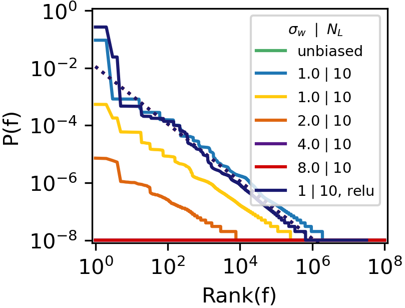
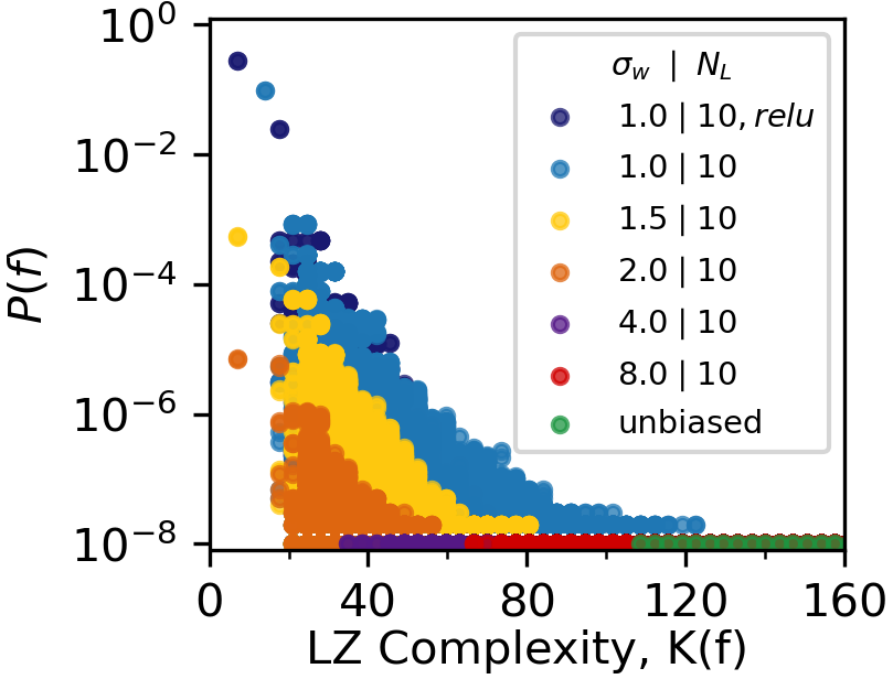
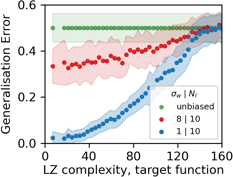
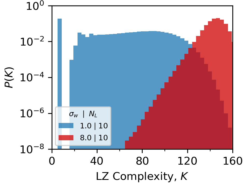
In Figures 1(a) and 1(b) we depict prior probabilities for functions defined on all inputs of a Boolean system upon random sampling of parameters of an FCN with 10 layers and hidden width 40 (which is large enough to be fully expressive for this system [17]), and activation functions. The simplicity bias in becomes weaker as the width of the Gaussian increases. By contrast, for ReLU activations, the bias in barely changes with (see Figure S3(a)). The effect of the decrease in simplicity bias on DNN generalization performance is demonstrated in Figure 1(c) for a DNN trained to zero error on a training set of size using advSGD (an SGD variant taken from [10]), and tested on the other inputs . The generalization error (the fraction of incorrect predictions on ) varies as a function of the complexity of the target function. Although all these DNNs exhibit simplicity bias, weaker forms of the bias correspond to significantly worse generalization on the simpler targets (see also Appendix J). For very complex targets, both networks perform poorly. Finally, we also show an unbiased learner, where functions are chosen uniformly at random with the proviso that they exactly fit the training set . Not surprisingly, given the functions that can fit , the performance of this unbiased learner is no better than random chance.
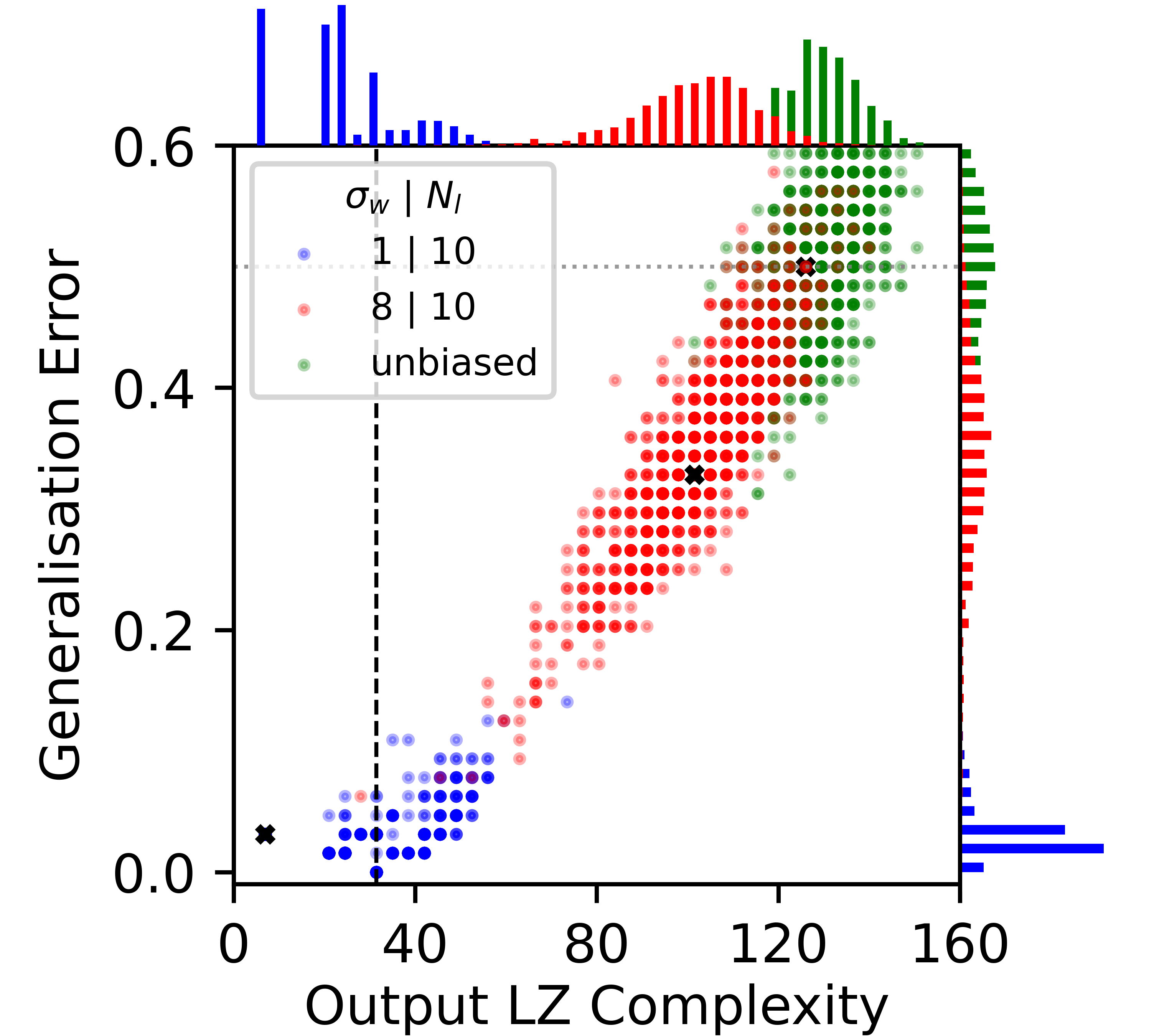
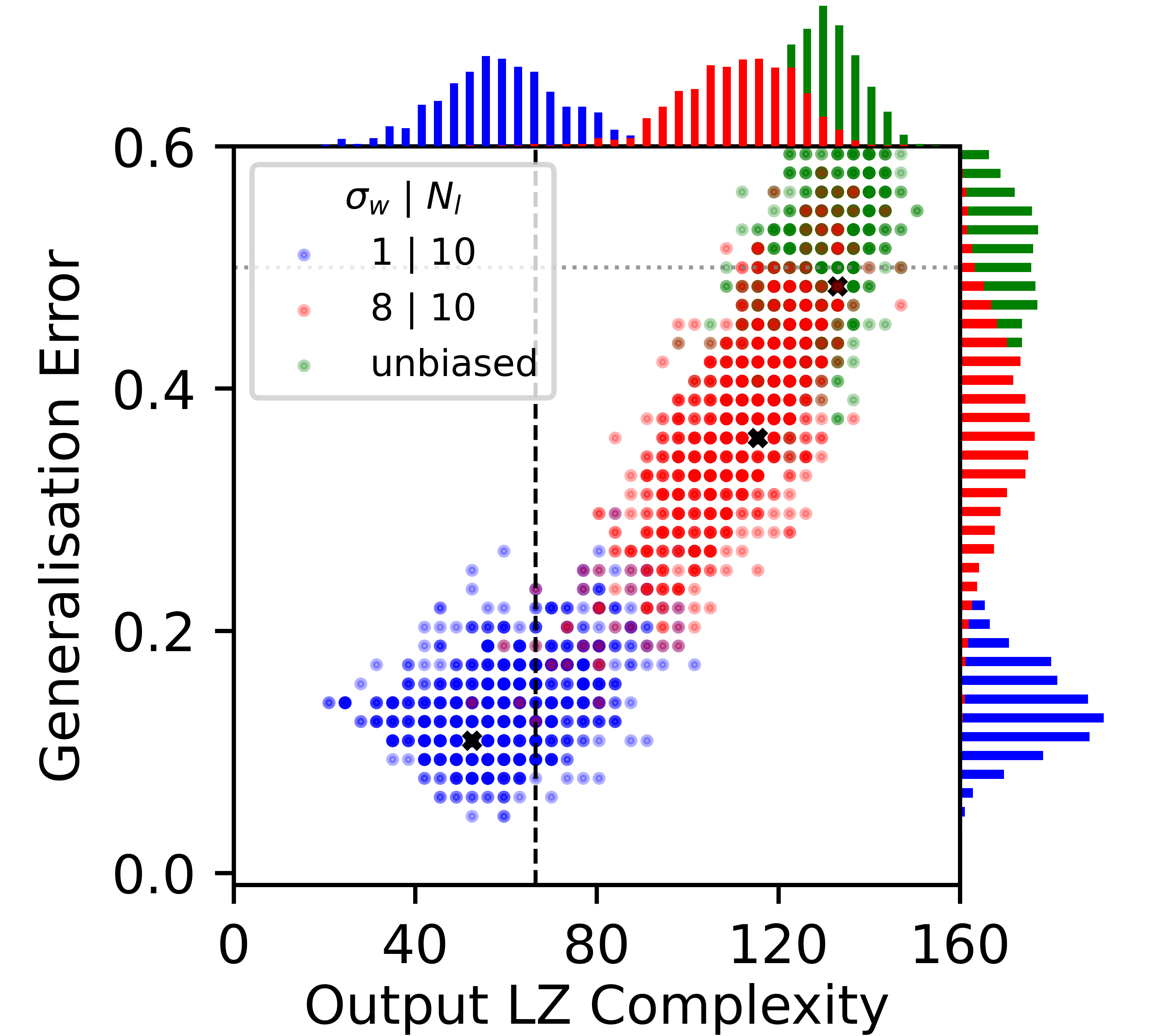
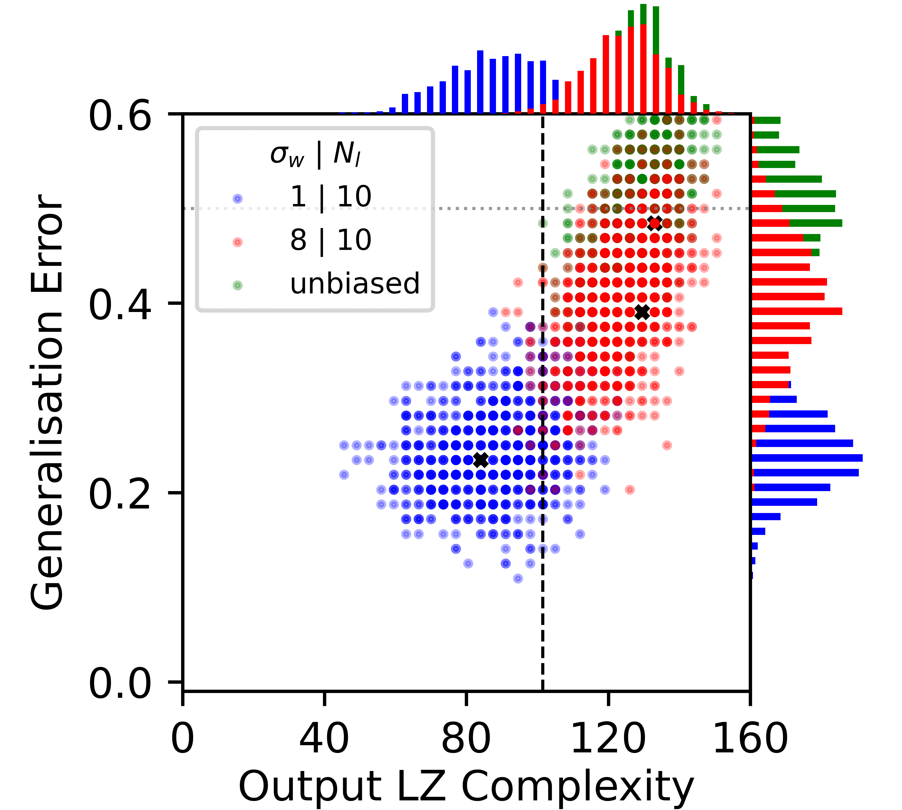
The scatter plots of Figure 1 (d)–(f) depict a more fine-grained picture of the behaviour of the SGD-trained networks for three different target functions. For each target, independent initialisations of the SGD optimiser, with initial parameters taken from , are used. The generalization error and complexity of each function found when the DNN first reaches zero training error are plotted. Since there are possible functions that give zero error on the training set , it is not surprising that the DNN converges to many different functions upon different random initialisations. For the network (where resembles that of ReLU networks) the most common function is typically simpler than the target. By contrast, the less biased network converges on functions that are typically more complex than the target. As the target itself becomes more complex, the relative difference between the two generalization errors decreases, because the strong inductive bias towards simple functions of the first network becomes less useful. No free lunch theorems for supervised learning tell us that when averaged over all target functions, the three learners above will perform equally badly [25, 26] (see also Section D.3).
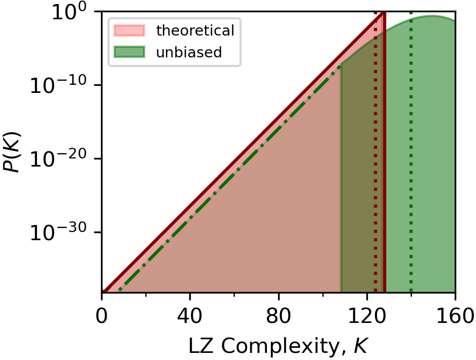
To understand why changes in the inductive bias towards simplicity that are small relative to the or so orders of magnitude scale on which varies (see also Figure S3(b)) nevertheless lead to such significant differences in generalization performance, we need another important ingredient, namely how the number of functions vary with complexity. Basic counting arguments imply that the number of strings of a fixed length that have complexity scales exponentially as [13]. Therefore, the vast majority of functions picked at random will have high complexity. This exponential growth of the number of functions with complexity can be captured in a more coarse-grained prior, the probability that the DNN expresses a function of complexity upon random sampling of parameters over a parameter initialisation function , which can also be written in terms of functions as , the weighted sum over the set of all functions with complexity . In Figure 1 (g) is shown for uniform random sampling of functions for samples using the LZ measure, and also for the theoretical ideal compressor with over all functions (see also Appendix I). In (h) we display the dramatic difference between the fully simplicity-biased and the less-biased . For the network with is nearly flat. This behaviour follows from the fact that the AIT coding-theorem like scaling [11, 10] of the prior over functions counters the growth in the number of functions. By contrast, for the more artefactual system, the simplicity bias is less strong. Even though there remains significant simplicity bias (we estimate that for the simplest functions, is about times higher than the mean probability ) this DNN is orders of magnitude more likely to throw up complex functions, an effect that SGD is unable to overcome.
The fact that the number of complex functions grows exponentially with complexity lies at the heart of the classical explanation of why a complex learning agent suffers from variance: It can too easily find many different functions that all fit the data. The marked differences in the generalization performance between the two networks observed in Figure 1 (c)–(f) can be therefore traced to differences in the inductive bias of the networks, as measured by the differences in their priors. The network is not simplicity biased enough to overcome the growth in the number of functions, and so it suffers from the classic problem of overfitting and large variance. By contrast, the system, and the nearly identical ReLU system, solve this problem because their inductive bias cancels the exponential growth in complex functions.
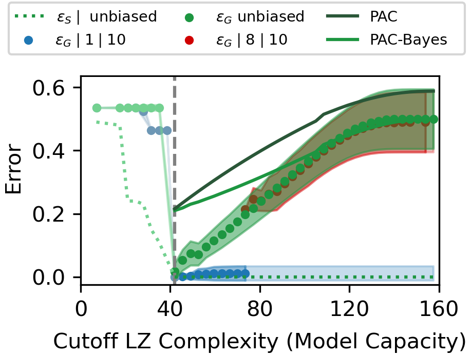
Artificially restricting model capacity To further illustrate the effect of inductive bias we create a K-learner that only allows functions with complexity to be learned and discards all others. As can be seen in Figure 1 (i), the learners typically cannot reach zero training error on the training set if is less than the target function complexity . For , zero training error can be reached and not surprisingly, the lowest generalization error occurs when . As the upper limit is increased, all three learning agents are more likely to make errors in predictions due to variance. The random learner has an error that grows linearly with . This behaviour can be understood with a classic PAC bound [6] where the generalization error (with confidence ) scales as , where is the size of the hypothesis class of all functions with ; the bound scales linearly in , as the error does (see Appendix G for further discussion including the more sophisticated PAC-Bayes bound [27, 28].). The generalization error for the DNN does not change much with for because the strong inductive bias towards simple solutions means access to higher complexity solutions doesn’t significantly change what the DNN converges on.
Calculating the Bayesian posterior and likelihood
To better understand the generalization behaviour observed in Figure 1 we apply Bayes’ rule, to calculate the Bayesian posterior from the prior , the likelihood , and the marginal likelihood . Since we condition on zero training error, the likelihood takes on a simple form. , while otherwise. For a fixed training set, all the variation in for , the set of all functions compatible with , comes from the prior since is constant. Therefore, in this Bayesian picture, the bias in the prior is translated over to the posterior.
The marginal likelihood also takes a relatively simple form for discrete functions, since . It is equivalent to the probability that the DNN obtains zero error on the training set upon random sampling of parameters, and so can be interpreted as a measure of the inductive bias towards the data. The Marginal-likelihood PAC-Bayes bound [28] makes a direct link to the generalization error which captures the intuition that, for a given , a better inductive bias towards the data (larger ) implies better performance (lower ).
One can also define the posterior probability , that a network trained with SGD (or another optimiser) on training set , when initialised with , converges on function . For simplicity, we take this probability at the epoch where the system first reaches zero training error. Note that in Figure 1 (d)–(f) it is this SGD-based posterior that we plot in the histograms at the top and sides of the plots, with functions grouped either by complexity, which we will call , or by generalization error , which we will call .
DNNs are typically trained by some form of SGD, and not by randomly sampling over parameters which is much less efficient. However, a recent study [29] which carefully compared the two posteriors has shown that to first order, , for many different data sets and DNN architectures. We demonstrate this close similarity in Figure S12 explicitly for our Boolean system. This evidence suggests that Bayesian posteriors calculated by random sampling of parameters, which are much simpler to analyze, can be used to understand the dominant behaviour of an SGD-trained DNN, even if, for example, hyperparameter tuning can lead to 2nd-order deviations between the two methods (see also Appendix A).
To test the predictive power of our Bayesian picture, we first define the function error as the fraction of incorrect labels produces on the full set of inputs. Next, we average Bayes’ rule over all training sets of size :
| (2) |
where the mean likelihood is the probability of a function obtaining zero error on a training set of size . In the second step, we approximate the average of the ratio with the ratio of the averages which should be accurate if is highly concentrated, as is expected if the training set is not too small.
Equation 2 is hard to calculate, so we coarse-grain it by grouping together functions by their complexity:
| (3) |
and in the second step make a decoupling approximation where we average the likelihood term over a small number of functions with complexity with lowest generalization error since the smallest errors in the sum dominate exponentially since for . We then multiply by , which takes into account the value of the prior and the multiplicity of functions at that , and normalise . For a given target, we make the ansatz that this decoupling approximation provides an estimate that scales as the true (averaged) posterior.
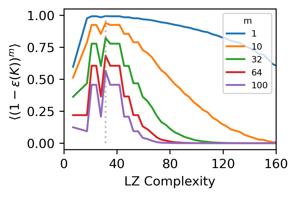
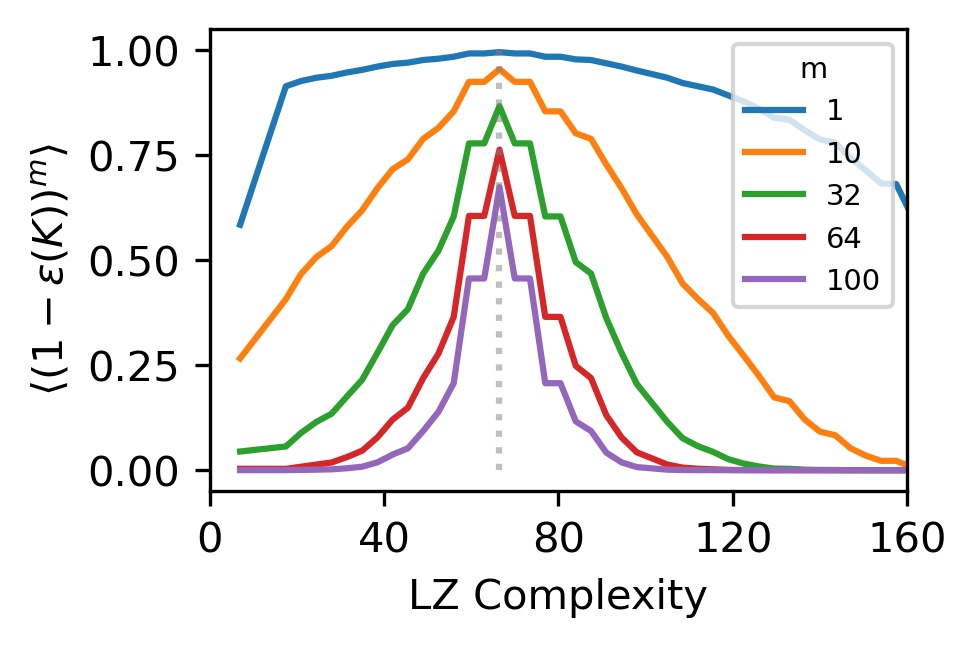
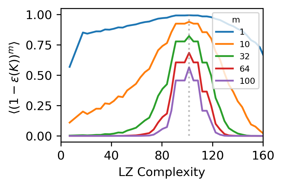
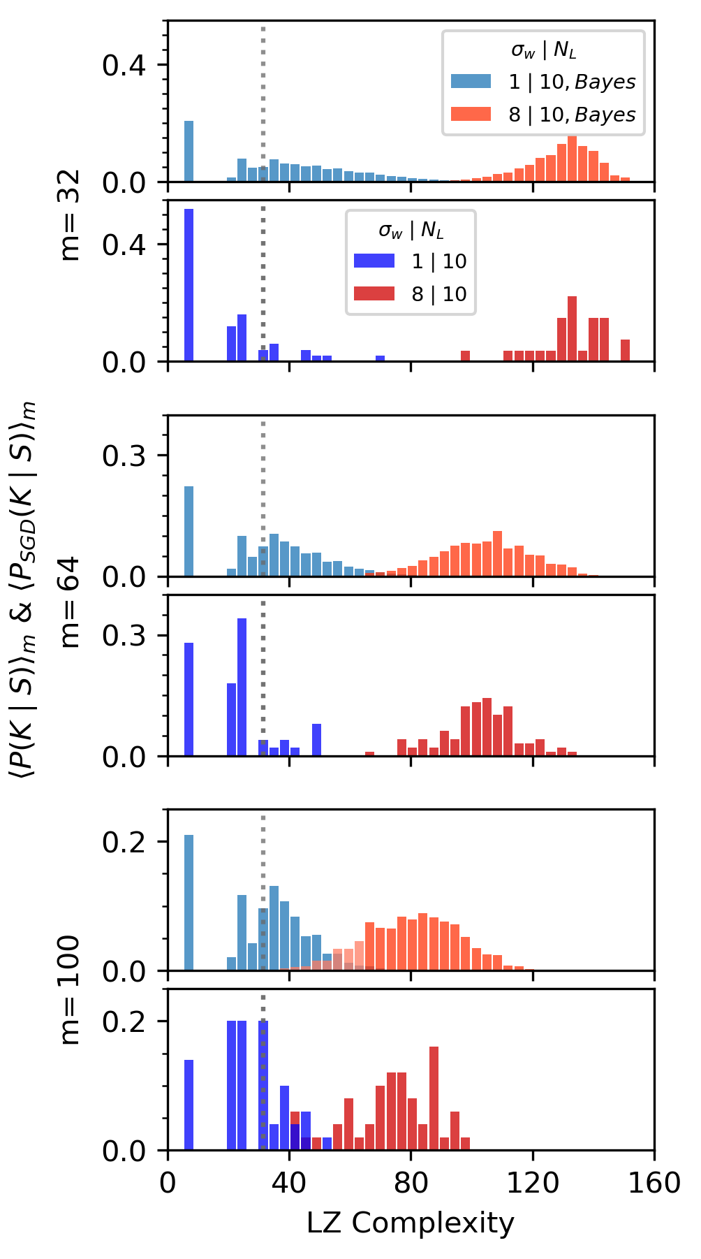
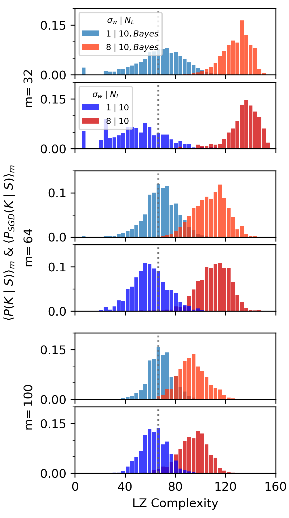
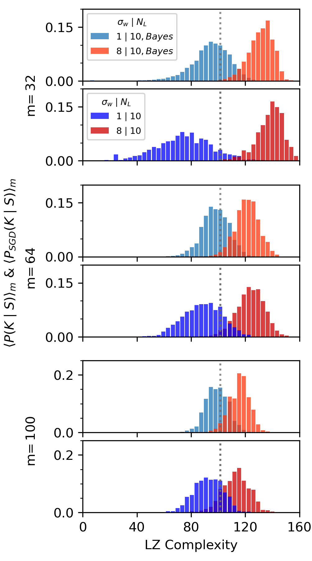
To test our approximations, we first plot, in Figure 2 (a)–(c), the likelihood term in Equation 3 for three different target functions. To obtain these curves, we considered a large number of functions (including all functions with up to 5 errors w.r.t. the target, with further functions sampled). For each complexity, we average this term over the functions with smallest Not surprisingly, functions close to the complexity of the target have the smallest error. These graphs help illustrate how the DNN interacts with data. As the training set size increases, functions that are most likely to be found upon training to zero training error are increasingly concentrated close to the complexity of the target function.
To test the decoupling approximation from Equation 3, we compare in Figure 2 (d)-(f) the posterior , calculated by multiplying the Bayesian likelihood curve from Figure 2 (a)–(c) with the two Bayesian priors from Figure 1 (h) and (i), to the posteriors calculated by advSGD [10] over a 1000 different parameter initialisations and training sets. It is remarkable to see how well the simple decoupling approximation performs across target functions and training set sizes. In Figures S10 and S11) we demonstrate the robustness of our approach by showing that using or functions does not change the predictions much. This success suggests that our simple approach captures the essence of the interaction between the data (measured by the likelihood, which is independent of the learning algorithm), and the DNN architecture (which is measured by the prior and is independent of the data).
We have therefore separated out two of the three parts of the tripartite scheme, which leaves the training algorithm. In the figures above our Bayesian approximation captures the dominant behaviour of an SGD-trained network. This correspondence is consistent with the results and arguments of [29]. We checked this further in Appendix K for a similar set-up using MSE loss, where Bayesian posteriors can be exactly calculated using Gaussian processes (GPs). At this scale of comparison, the direct Bayesian GP calculation closely matches SGD based results.
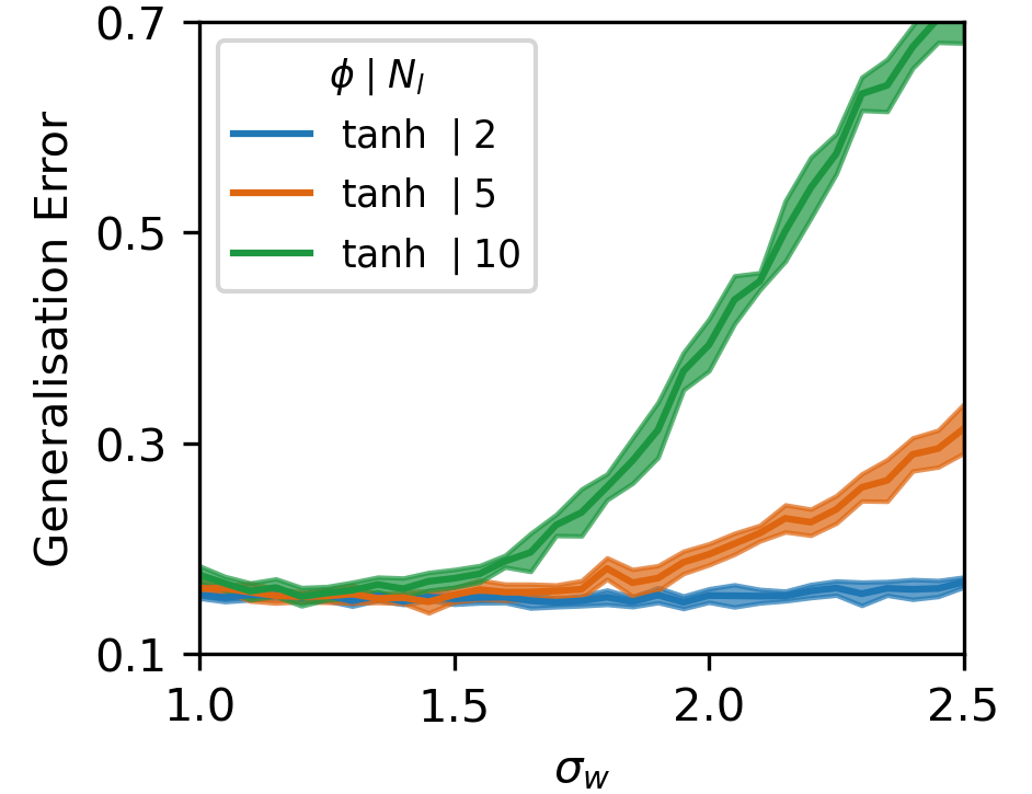
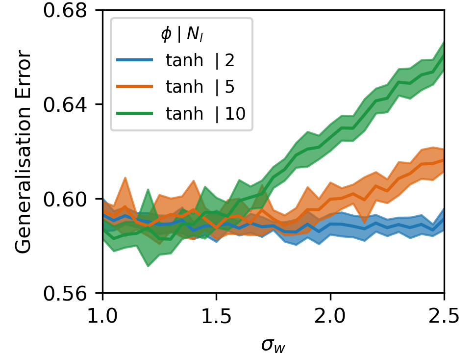
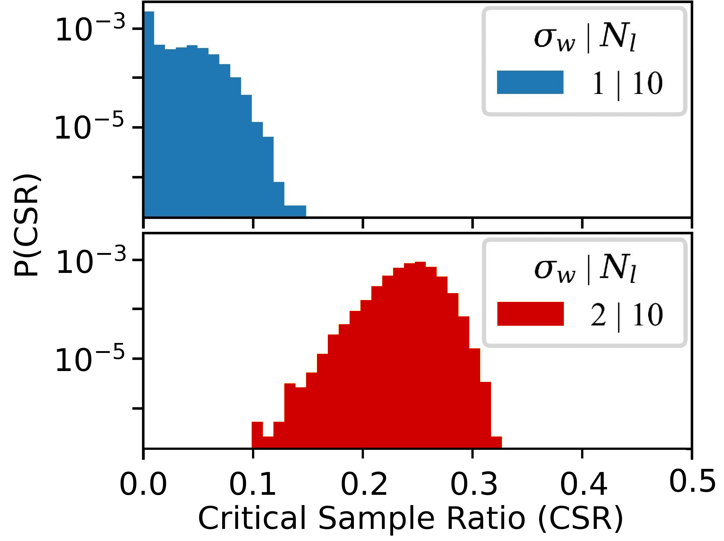
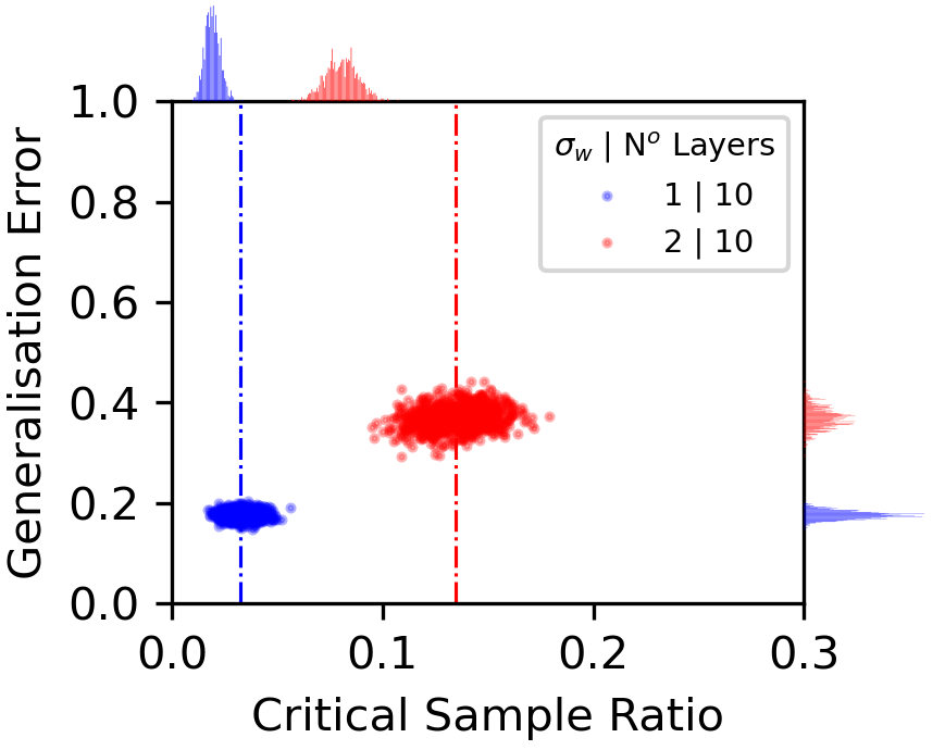
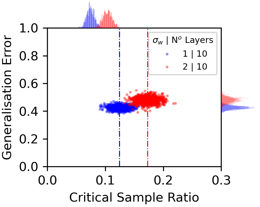
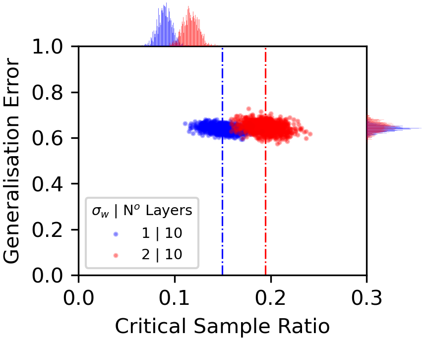
Beyond the Boolean model: MINST CIFAR-10 Can the principles worked out for the Boolean system be observed in larger systems that are closer to the standard practice of DNNs? To this end, we show, in Figure 3 (a) and (b) how the generalization error for the popular image datasets MNIST and CIFAR-10 changes as a function of the initial parameter width and the number of layers for a standard FCN, trained with SGD on cross-entropy loss with activation functions. Larger and larger push the system deeper into the chaotic regime [22, 23] and result in decreasing generalization performance, similar to what we observe for the Boolean system for relatively simple targets. In Figure 3, we plot the prior over complexity for a complexity measure called the critical sample ratio (CSR) [14], an estimate of the density of decision boundaries that should be appropriate for this problem. Again, increasing greatly increases the prior probability that the DNN produces more complex functions upon random sampling of parameters. Thus the decrease in generalization performance is consistent with the inductive bias of the network becoming less simplicity biased, and therefore less well aligned with structure in the data. Indeed, datasets such as MNIST and CIFAR-10 are thought to be relatively simple [30, 31].
These patterns are further illustrated in Figure 3 (d)–(f) where we show scatterplots of generalization error v.s. CSR complexity for three target functions that vary in complexity (here obtained by corrupting labels). The qualitative behaviour is similar to that observed for the Boolean system in Fig 1. The more simplicity-biased networks perform significantly better on the simpler targets, but the difference with the less simplicity-biased network decreases for more complex targets. While we are unable to directly calculate the likelihoods because these systems are too big, we argue that the strong similarities to our simpler model system suggest that the same basic principles of inductive bias are at work here.
Discussion of Occam’s razor in DNNs: In order to generalize, high capacity models need a clear inductive bias towards functions that perform well on the data being studied [32]. Here we showed that one key to the success of modern DNNs is a specific intrinsic inductive bias of the form which can counteract the growth of the number of functions with complexity. Such a bias towards simplicity suggests that DNNs have a very specific kind of inbuilt Occam’s razor (see Appendix D for background on Occam’s razor(s)). Even a rather modest reduction in the inductive bias –which might still qualify as Occam’s razor– can lead to dramatic decreases in performance. Many kernel methods also have high capacity, implying that they require a similar inductive bias to prevent them from also being caught out by the exponential growth of the number of functions with complexity.
There may be links to more formal arguments in AIT relating to the optimality of Solomonoff induction which is based on a universal prior that both takes into account all hypotheses consistent with the data (Epicurus’s principle), but prioritises the (Kolmogorov) simpler ones [13, 33]. Similarly, the (nearly) flat means the DNN has access to hypotheses with a large range of complexities that can then interact with data. Needless to say, much more work is needed to work out whether these connections are superficial or profound (see also Section D.4).
We were not able to significantly increase the bias towards simplicity in DNNs. Too strong a bias towards simplicity can mean a loss of versatility because complex functions become hard to find [34, 12].
The methods used in this paper work well for classification of discrete functions. An important further piece of research, where kernel methods may play a more central role, is to study the inductive biases for regression problems with continuous functions.
While we have explored some key ingredients, the full question of why DNNs generalize so well remains open. Understanding what the extra 2nd-order effects of hyperparameter tuning etc. are, or how feature learning (which is not present in Bayesian GPs) improves generalization are important problems that our methods are unlikely to solve. Our results do not preclude the fact that SGD optimization itself can also introduce useful inductive biases (see also Appendix A). Simplicity bias is one of many inductive biases that DNNs likely exhibit. Much of the exciting recent progress in foundation models such as GPT-4 likely arises from inductive biases well beyond just simplicity, although simplicity bias plays an important role for such models [12]. Systematically studying and understanding how these biases interact with data remains one of the key challenges in modern machine learning.
Finally, our observations about inductive bias can be inverted to reveal properties of the data on which DNNs are successful at learning. For example, data cannot be too complex. Furthermore, the remarkable success of DNNs on a broad range of scientific problems [35, 36, 37, 38] suggests that their inductive biases must recapitulate something deep about the structure of the natural world [15]. Understanding why DNNs choose the solutions they do may, in turn, generate profound insights into nature itself.
Acknowledgements.
We thank Satwik Bhattamishra, Kamal Dingle, Nayara Fonseca, and Yoonsoo Nam for helpful discussions.References
- [1] LeCun, Y., Bengio, Y. & Hinton, G. Deep learning. Nature 521, 436 (2015).
- [2] Schmidhuber, J. Discovering neural nets with low kolmogorov complexity and high generalization capability. Neural Networks 10, 857–873 (1997).
- [3] Breiman, L. Reflections after refereeing papers for nips. In The Mathematics of Generalization, 11–15 (Addison-Wesley, 1995).
- [4] Zdeborová, L. Understanding deep learning is also a job for physicists. Nature Physics 1–3 (2020).
- [5] Dyson, F. A meeting with enrico fermi. Nature 427, 297–297 (2004).
- [6] Shalev-Shwartz, S. & Ben-David, S. Understanding machine learning: From theory to algorithms (Cambridge university press, 2014).
- [7] Zhang, C., Bengio, S., Hardt, M., Recht, B. & Vinyals, O. Understanding deep learning requires rethinking generalization. arXiv preprint arXiv:1611.03530 (2016).
- [8] Cybenko, G. Approximation by superpositions of a sigmoidal function. Mathematics of control, signals and systems 2, 303–314 (1989).
- [9] Hornik, K. Approximation capabilities of multilayer feedforward networks. Neural networks 4, 251–257 (1991).
- [10] Valle-Pérez, G., Camargo, C. Q. & Louis, A. A. Deep learning generalizes because the parameter-function map is biased towards simple functions. arXiv preprint arXiv:1805.08522 (2018).
- [11] Dingle, K., Camargo, C. Q. & Louis, A. A. Input–output maps are strongly biased towards simple outputs. Nature Communications 9, 1–7 (2018).
- [12] Bhattamishra, S., Patel, A., Kanade, V. & Blunsom, P. Simplicity bias in transformers and their ability to learn sparse boolean functions. arXiv preprint arXiv:2211.12316 (2022).
- [13] Li, M. & Vitanyi, P. An introduction to Kolmogorov complexity and its applications (Springer-Verlag New York Inc, 2008).
- [14] Arpit, D. et al. A closer look at memorization in deep networks. arXiv preprint arXiv:1706.05394 (2017).
- [15] Lin, H. W., Tegmark, M. & Rolnick, D. Why does deep and cheap learning work so well? Journal of Statistical Physics 168, 1223–1247 (2017).
- [16] De Palma, G., Kiani, B. T. & Lloyd, S. Random deep neural networks are biased towards simple functions. arXiv preprint arXiv:1812.10156 (2018).
- [17] Mingard, C. et al. Neural networks are a priori biased towards boolean functions with low entropy. arXiv preprint arXiv:1909.11522 (2019).
- [18] Kalimeris, D. et al. Sgd on neural networks learns functions of increasing complexity. Advances in neural information processing systems 32 (2019).
- [19] Huh, M. et al. The low-rank simplicity bias in deep networks. arXiv preprint arXiv:2103.10427 (2021).
- [20] Farhang, A. R., Bernstein, J. D., Tirumala, K., Liu, Y. & Yue, Y. Investigating generalization by controlling normalized margin. In International Conference on Machine Learning, 6324–6336 (PMLR, 2022).
- [21] Chiang, P.-y. et al. Loss landscapes are all you need: Neural network generalization can be explained without the implicit bias of gradient descent. In The Eleventh International Conference on Learning Representations (2023).
- [22] Poole, B., Lahiri, S., Raghu, M., Sohl-Dickstein, J. & Ganguli, S. Exponential expressivity in deep neural networks through transient chaos. In Advances in neural information processing systems, 3360–3368 (2016).
- [23] Schoenholz, S. S., Gilmer, J., Ganguli, S. & Sohl-Dickstein, J. Deep information propagation. In International Conference on Learning Representations (2017). URL https://openreview.net/forum?id=H1W1UN9gg.
- [24] Yang, G. & Salman, H. A fine-grained spectral perspective on neural networks. arXiv preprint arXiv:1907.10599 (2019).
- [25] Schaffer, C. A conservation law for generalization performance. In Machine Learning Proceedings 1994, 259–265 (Elsevier, 1994).
- [26] Wolpert, D. H. The lack of a priori distinctions between learning algorithms. Neural computation 8, 1341–1390 (1996).
- [27] McAllester, D. A. Some pac-bayesian theorems. Machine Learning 37, 355–363 (1999).
- [28] Valle-Pérez, G. & Louis, A. A. Generalization bounds for deep learning. arXiv preprint arXiv:2012.04115 (2020).
- [29] Mingard, C., Valle-Pérez, G., Skalse, J. & Louis, A. A. Is sgd a bayesian sampler? well, almost. Journal of Machine Learning Research 22, 1–64 (2021).
- [30] Spigler, S., Geiger, M. & Wyart, M. Asymptotic learning curves of kernel methods: empirical data versus teacher–student paradigm. Journal of Statistical Mechanics: Theory and Experiment 2020, 124001 (2020).
- [31] Goldt, S., Mézard, M., Krzakala, F. & Zdeborová, L. Modelling the influence of data structure on learning in neural networks. arXiv preprint arXiv:1909.11500 (2019).
- [32] Mitchell, T. M. The need for biases in learning generalizations (rutgers computer science tech. rept. cbm-tr-117). Rutgers University (1980).
- [33] Rathmanner, S. & Hutter, M. A philosophical treatise of universal induction. Entropy 13, 1076–1136 (2011).
- [34] Shah, H., Tamuly, K., Raghunathan, A., Jain, P. & Netrapalli, P. The pitfalls of simplicity bias in neural networks. Advances in Neural Information Processing Systems 33, 9573–9585 (2020).
- [35] Ching, T. et al. Opportunities and obstacles for deep learning in biology and medicine. Journal of The Royal Society Interface 15, 20170387 (2018).
- [36] Mehta, P. et al. A high-bias, low-variance introduction to machine learning for physicists. Physics reports 810, 1–124 (2019).
- [37] Carleo, G. et al. Machine learning and the physical sciences. Reviews of Modern Physics 91, 045002 (2019).
- [38] Karniadakis, G. E. et al. Physics-informed machine learning. Nature Reviews Physics 3, 422–440 (2021).
- [39] Hanin, B. Universal function approximation by deep neural nets with bounded width and relu activations. Mathematics 7, 992 (2019).
- [40] Belkin, M., Hsu, D., Ma, S. & Mandal, S. Reconciling modern machine learning practice and the bias-variance trade-off. arXiv preprint arXiv:1812.11118 (2018).
- [41] Loog, M., Viering, T., Mey, A., Krijthe, J. H. & Tax, D. M. A brief prehistory of double descent. Proceedings of the National Academy of Sciences 117, 10625–10626 (2020).
- [42] Mei, S. & Montanari, A. The generalization error of random features regression: Precise asymptotics and double descent curve. arXiv preprint arXiv:1908.05355 (2019).
- [43] Hastie, T., Montanari, A., Rosset, S. & Tibshirani, R. Surprises in high-dimensional ridgeless least squares interpolation. arXiv preprint: arXiv:1903.08560 (2019).
- [44] Advani, M. S., Saxe, A. M. & Sompolinsky, H. High-dimensional dynamics of generalization error in neural networks. Neural Networks 132, 428–446 (2020).
- [45] McAllester, D. A. Some pac-bayesian theorems. In Proceedings of the eleventh annual conference on Computational learning theory, 230–234 (ACM, 1998).
- [46] Harzli, O. E., Valle-Pérez, G. & Louis, A. A. Double-descent curves in neural networks: a new perspective using gaussian processes. arXiv preprint arXiv:2102.07238 (2021).
- [47] Belkin, M., Ma, S. & Mandal, S. To understand deep learning we need to understand kernel learning. In Dy, J. & Krause, A. (eds.) Proceedings of the 35th International Conference on Machine Learning, vol. 80 of Proceedings of Machine Learning Research, 541–549 (PMLR, Stockholmsmässan, Stockholm Sweden, 2018). URL http://proceedings.mlr.press/v80/belkin18a.html.
- [48] Neal, R. M. Priors for infinite networks (tech. rep. no. crg-tr-94-1). University of Toronto (1994).
- [49] Jacot, A., Gabriel, F. & Hongler, C. Neural tangent kernel: Convergence and generalization in neural networks. In Advances in neural information processing systems, 8571–8580 (2018).
- [50] Lee, J. et al. Deep neural networks as gaussian processes. arXiv preprint arXiv:1711.00165 (2017).
- [51] Matthews, A. G. d. G., Rowland, M., Hron, J., Turner, R. E. & Ghahramani, Z. Gaussian process behaviour in wide deep neural networks. arXiv preprint arXiv:1804.11271 (2018).
- [52] Novak, R. et al. Bayesian convolutional neural networks with many channels are gaussian processes. arXiv preprint arXiv:1810.05148 (2018).
- [53] Garriga-Alonso, A., Rasmussen, C. E. & Aitchison, L. Deep convolutional networks as shallow gaussian processes. In International Conference on Learning Representations (2019). URL https://openreview.net/forum?id=Bklfsi0cKm.
- [54] Yang, G. Wide feedforward or recurrent neural networks of any architecture are gaussian processes. In Advances in Neural Information Processing Systems, 9951–9960 (2019).
- [55] Yang, G. & Hu, E. J. Feature learning in infinite-width neural networks. arXiv preprint arXiv:2011.14522 (2020).
- [56] Lee, J. et al. Finite versus infinite neural networks: an empirical study. Advances in Neural Information Processing Systems 33, 15156–15172 (2020).
- [57] Geiger, M., Spigler, S., Jacot, A. & Wyart, M. Disentangling feature and lazy training in deep neural networks. Journal of Statistical Mechanics: Theory and Experiment 2020, 113301 (2020).
- [58] Roberts, D. A., Yaida, S. & Hanin, B. The principles of deep learning theory (Cambridge University Press, 2022).
- [59] Oymak, S., Fabian, Z., Li, M. & Soltanolkotabi, M. Generalization guarantees for neural networks via harnessing the low-rank structure of the jacobian. arXiv preprint arXiv:1906.05392 (2019).
- [60] Lou, Y., Mingard, C., Nam, Y. & Hayou, S. Feature learning and signal propagation in deep neural networks (2021). URL https://arxiv.org/abs/2110.11749.
- [61] Baratin, A. et al. Implicit regularization via neural feature alignment. In International Conference on Artificial Intelligence and Statistics, 2269–2277 (PMLR, 2021).
- [62] Keskar, N. S., Mudigere, D., Nocedal, J., Smelyanskiy, M. & Tang, P. T. P. On large-batch training for deep learning: Generalization gap and sharp minima. CoRR abs/1609.04836 (2016). URL http://arxiv.org/abs/1609.04836. eprint 1609.04836.
- [63] Goyal, P. et al. Accurate, large minibatch sgd: Training imagenet in 1 hour. arXiv preprint arXiv:1706.02677 (2017).
- [64] Hoffer, E., Hubara, I. & Soudry, D. Train longer, generalize better: closing the generalization gap in large batch training of neural networks. In Advances in Neural Information Processing Systems, 1731–1741 (2017).
- [65] Smith, S. L., Kindermans, P.-J., Ying, C. & Le, Q. V. Don’t decay the learning rate, increase the batch size. arXiv preprint arXiv:1711.00489 (2017).
- [66] Geiping, J., Goldblum, M., Pope, P. E., Moeller, M. & Goldstein, T. Stochastic training is not necessary for generalization. arXiv preprint arXiv:2109.14119 (2021).
- [67] Izmailov, P., Podoprikhin, D., Garipov, T., Vetrov, D. & Wilson, A. G. Averaging weights leads to wider optima and better generalization. arXiv preprint arXiv:1803.05407 (2018).
- [68] Wilson, A. G. & Izmailov, P. Bayesian deep learning and a probabilistic perspective of generalization. Advances in neural information processing systems 33, 4697–4708 (2020).
- [69] Soudry, D., Hoffer, E., Nacson, M. S., Gunasekar, S. & Srebro, N. The implicit bias of gradient descent on separable data. The Journal of Machine Learning Research 19, 2822–2878 (2018).
- [70] Bernstein, J., Farhang, A. & Yue, Y. Kernel interpolation as a bayes point machine. arXiv (2021).
- [71] Bartlett, P. L., Long, P. M., Lugosi, G. & Tsigler, A. Benign overfitting in linear regression. Proceedings of the National Academy of Sciences 117, 30063–30070 (2020).
- [72] Belkin, M. Fit without fear: remarkable mathematical phenomena of deep learning through the prism of interpolation. arXiv preprint arXiv:2105.14368 (2021).
- [73] Mallinar, N. et al. Benign, tempered, or catastrophic: A taxonomy of overfitting. arXiv preprint arXiv:2207.06569 (2022).
- [74] Bordelon, B., Canatar, A. & Pehlevan, C. Spectrum dependent learning curves in kernel regression and wide neural networks. In International Conference on Machine Learning, 1024–1034 (PMLR, 2020).
- [75] Canatar, A., Bordelon, B. & Pehlevan, C. Spectral bias and task-model alignment explain generalization in kernel regression and infinitely wide neural networks. Nature communications 12, 1–12 (2021).
- [76] Cui, H., Loureiro, B., Krzakala, F. & Zdeborová, L. Generalization error rates in kernel regression: The crossover from the noiseless to noisy regime. Advances in Neural Information Processing Systems 34, 10131–10143 (2021).
- [77] Simon, J. B., Dickens, M. & DeWeese, M. R. Neural tangent kernel eigenvalues accurately predict generalization. arXiv preprint arXiv:2110.03922 (2021).
- [78] Li, H., Kadav, A., Durdanovic, I., Samet, H. & Graf, H. P. Pruning filters for efficient convnets. arXiv preprint arXiv:1608.08710 (2016).
- [79] Frankle, J. & Carbin, M. The lottery ticket hypothesis: Finding sparse, trainable neural networks. arXiv preprint arXiv:1803.03635 (2018).
- [80] Hein, M. & Audibert, J.-Y. Intrinsic dimensionality estimation of submanifolds in rd. In Proceedings of the 22nd international conference on Machine learning, 289–296 (2005).
- [81] Rahaman, N. et al. On the spectral bias of neural networks. In International Conference on Machine Learning, 5301–5310 (PMLR, 2019).
- [82] Refinetti, M., Ingrosso, A. & Goldt, S. Neural networks trained with sgd learn distributions of increasing complexity. arXiv preprint arXiv:2211.11567 (2022).
- [83] Xu, Z.-Q. J., Zhang, Y. & Luo, T. Overview frequency principle/spectral bias in deep learning. arXiv preprint arXiv:2201.07395 (2022).
- [84] Domingos, P. The role of occam’s razor in knowledge discovery. Data mining and knowledge discovery 3, 409–425 (1999).
- [85] Geirhos, R. et al. Shortcut learning in deep neural networks. Nature Machine Intelligence 2, 665–673 (2020).
- [86] Levin, L. Laws of information conservation (nongrowth) and aspects of the foundation of probability theory. Problemy Peredachi Informatsii 10, 30–35 (1974).
- [87] Dingle, K., Pérez, G. V. & Louis, A. A. Generic predictions of output probability based on complexities of inputs and outputs. Scientific Reports 10, 1–9 (2020).
- [88] Camargo, C. Q. & Louis, A. A. Boolean threshold networks as models of genotype-phenotype maps. In Complex Networks XI, 143–155 (Springer, 2020).
- [89] Johnston, I. G. et al. Symmetry and simplicity spontaneously emerge from the algorithmic nature of evolution. Proceedings of the National Academy of Sciences 119, e2113883119 (2022).
- [90] Lempel, A. & Ziv, J. On the complexity of finite sequences. IEEE Transactions on information theory 22, 75–81 (1976).
- [91] Huang, H. Induced subgraphs of hypercubes and a proof of the sensitivity conjecture. Annals of Mathematics 190, 949–955 (2019).
- [92] Mohanty, V. & Louis, A. A. Robustness and stability of spin-glass ground states to perturbed interactions. Physical Review E 107, 014126 (2023).
- [93] Hayou, S., Doucet, A. & Rousseau, J. Mean-field behaviour of neural tangent kernel for deep neural networks. arXiv preprint arXiv:1905.13654 (2019).
- [94] Baker, A. Simplicity. Stanford Encyclopedia of Philosophy (2004).
- [95] Sober, E. Ockham’s razors (Cambridge University Press, 2015).
- [96] Newton is probably echoing Duns Scotus’s who wrote: we should always posit fewer things when the appearances can be saved thereby . . . therefore in positing more things we should always indicate the manifest necessity on account of which so many things are posited. from Questions on the Books of Metaphysics of Aristotle, Book VIII, Q.1, n.22.
- [97] Einstein, A. On the method of theoretical physics. Philosophy of science 1, 163–169 (1934).
- [98] Popper, K. R. Logik der Forschung (JCB Mohr Tübingen, 1989).
- [99] MacKay, D. J. Information theory, inference and learning algorithms (Cambridge university press, 2003).
- [100] Kelly, K. T. A new solution to the puzzle of simplicity. Philosophy of Science 74, 561–573 (2007).
- [101] Bargagli Stoffi, F. J., Cevolani, G. & Gnecco, G. Simple models in complex worlds: Occam’s razor and statistical learning theory. Minds and Machines 32, 13–42 (2022).
- [102] Harman, G. & Kulkarni, S. Reliable Reasoning: Induction and Statistical Learning Theory (MIT Press, 2007).
- [103] Blumer, A., Ehrenfeucht, A., Haussler, D. & Warmuth, M. K. Occam’s razor. Information processing letters 24, 377–380 (1987).
- [104] Pearl, J. On the connection between the complexity and credibility of inferred models. International Journal of General System 4, 255–264 (1978).
- [105] Schaffer, C. Overfitting avoidance as bias. Machine learning 10, 153–178 (1993).
- [106] Wolpert, D. H. & Macready, W. G. No free lunch theorems for optimization. IEEE transactions on evolutionary computation 1, 67–82 (1997).
- [107] Solomonoff, R. J. A preliminary report on a general theory of inductive inference (Citeseer, 1960).
- [108] Solomonoff, R. J. A formal theory of inductive inference. part i. Information and control 7, 1–22 (1964).
- [109] Kolmogorov, A. N. Three approaches to the quantitative definition of information. International journal of computer mathematics 2, 157–168 (1968).
- [110] Chaitin, G. J. On the simplicity and speed of programs for computing infinite sets of natural numbers. Journal of the ACM (JACM) 16, 407–422 (1969).
- [111] A prefix Turing machine can be constructed as a Turing machine with one unidirectional (where the head can only move from left to right) input tape, one unidirectional output tape, and a bidirectional (the head can only move in either direction) work tape. Input tapes are read-only, and output tapes are write-only. All tapes are binary (no blank symbol), and work tapes are initially filled with zeros. For a program to be valid, the prefix UTM must halt with the input head at some point on the input tape. As the input head can only move left to right, it can never access further symbols on the input tape, and thus no valid program can be the prefix of any other valid program. [13].
- [112] Bauwens, B. Relating and contrasting plain and prefix kolmogorov complexity. Theory of Computing Systems 58, 482–501 (2016).
- [113] Kirchherr, W., Li, M. & Vitányi, P. The miraculous universal distribution. The Mathematical Intelligencer 19, 7–15 (1997).
- [114] Hutter, M. A theory of universal artificial intelligence based on algorithmic complexity. arXiv preprint cs/0004001 (2000).
- [115] Hutter, M. Universal artificial intelligence: Sequential decisions based on algorithmic probability (Springer Science & Business Media, 2004).
- [116] Schmidhuber, J. The speed prior: a new simplicity measure yielding near-optimal computable predictions. In International conference on computational learning theory, 216–228 (Springer, 2002).
- [117] Rissanen, J. Modeling by shortest data description. Automatica 14, 465–471 (1978).
- [118] Grünwald, P. D. The minimum description length principle (MIT Press, 2007).
- [119] Lattimore, T. & Hutter, M. No free lunch versus occam’s razor in supervised learning. In Algorithmic Probability and Friends. Bayesian Prediction and Artificial Intelligence, 223–235 (Springer, 2013).
- [120] Sterkenburg, T. F. Solomonoff prediction and occam’s razor. Philosophy of Science 83, 459–479 (2016).
- [121] Sterkenburg, T. F. Universal prediction: A philosophical investigation (University of Groningen, 2018).
- [122] Neth, S. A dilemma for solomonoff prediction. Philosophy of Science 1–25 (2022).
- [123] Christopher De Sa. Lecture 12: Bias-variance tradeoff. https://www.cs.cornell.edu/courses/cs4780/2018fa/lectures/lecturenote12.html (2018).
- [124] Kohavi, R., Wolpert, D. H. et al. Bias plus variance decomposition for zero-one loss functions. In ICML, vol. 96, 275–83 (1996).
- [125] Domingos, P. A unified bias-variance decomposition. In Proceedings of 17th international conference on machine learning, 231–238 (Morgan Kaufmann Stanford, 2000).
- [126] Geurts, P. Bias vs variance decomposition for regression and classification. In Data mining and knowledge discovery handbook, 733–746 (Springer, 2009).
- [127] McAllester, D. A. Pac-bayesian model averaging. In Proceedings of the twelfth annual conference on Computational learning theory, 164–170 (1999).
- [128] Amigó, J. M., Szczepański, J., Wajnryb, E. & Sanchez-Vives, M. V. Estimating the entropy rate of spike trains via lempel-ziv complexity. Neural Computation 16, 717–736 (2004).
- [129] Lesne, A., Blanc, J.-L. & Pezard, L. Entropy estimation of very short symbolic sequences. Physical Review E 79, 046208 (2009).
- [130] Matthews, A. G. d. G., Hron, J., Turner, R. E. & Ghahramani, Z. Sample-then-optimize posterior sampling for bayesian linear models. In NeurIPS Workshop on Advances in Approximate Bayesian Inference (2017).
- [131] http://yann.lecun.com/exdb/mnist/.
- [132] https://www.cs.toronto.edu/~kriz/cifar.html.
- [133] Krueger, D. et al. Deep nets don’t learn via memorization. International Conference on Learning Representations Workshop (2017). URL https://openreview.net/forum?id=HJC2SzZCW.
- [134] Nye, M. & Saxe, A. Are efficient deep representations learnable? arXiv preprint arXiv:1807.06399 (2018).
Appendix A Background literature on generalization in DNNs
In an opinionated 1995 commentary entitled “Reflections after refereeing for NIPS [NeurIPS]”[3], the influential late statistician Leo Breiman wrote:
There are many important questions regarding neural networks which are largely unanswered. There seem to be conflicting stories regarding the following issues:
- 1.
Why don’t heavily parameterized neural networks overfit the data?
- 2.
What is the effective number of parameters?
- 3.
Why doesn’t backpropagation head for a poor local minima?
- 4.
When should one stop the backpropagation and use the current parameters?
In spite of enormous technical advances in the use of neural networks over the ensuing 28 years since Breiman’s paper was written, these basic theoretical questions remain surprisingly relevant. Issues 1 and 3 were famously highlighted in 2016 by Zhang et al. [7] who demonstrated that AlexNet, a convolutional neural network (CNN) architecture, can obtain 100% accuracy on CIFAR10 for both randomised and non-randomised labels. Given that DNNs were known to have extremely high expressivity/large capacity [7, 8, 9, 39], it is perhaps not surprising that they can in principle fit randomised labels on images, which is captured by a measure of capacity called Rademacher complexity. What was perhaps more surprising than their high Rademacher complexity was how efficient SGD is at finding these complex solutions for randomized data. The main impact of the Zhang et al. [7] paper, however, was not its illustration of the power of SGD, but rather the evocative way it framed and popularised, for a new generation of researchers, Breiman’s big question (1) of why DNNs generalise despite their high expressivity/capacity. Their work can be interpreted as demonstrating that DNNs can easily “memorize” randomised data. For such solutions, generalization performance should be no better than random chance. This then begs the question: given that DNNs can easily find these memorized solutions, why do they instead normally converge to solutions that do generalize well? The authors demonstrated that explicit regularisation techniques (e.g. weight decay, dropout) were not necessary for DNNs to achieve these feats, further confounding the common intuition that regularization is needed to avoid overfitting. For our purposes, a key takeaway from their work is the demonstration that the good inductive bias observed in DNNs is something quite basic to how they operate.
Another study that captured the broader imagination was by Belkin et al. [40] who showed that DNNs (and related kernel methods) exhibit a ‘double-descent” phenomenon: In the under-parameterised regime the generalization error exhibits the classical “U-shaped” bias-variance tradeoff that peaks when the number of parameters is equal to the number of data points. In the overparameterized regime, the generalization error decreases (the second or “double” descent) with increasing ratio of parameters to data points down to some minimal risk (dependent on the dataset and architecture). Again, while the phenomenon of double descent (and even multiple descent) has a much longer history in machine learning, see e.g. [41] for some historical comments, the Belkin et al. paper [40] played an important role in popularising and framing the question of why DNNs behave so differently from the classical expectations of statistical learning theory. This paper also stimulated a number of follow-on works, including a series of important papers that used random matrix theory (RMT) techniques to analytically calculate the generalization error through the whole double-descent regime, albeit for typically simpler architectures, e.g. a two-layer neural network with random first-layer weights, and a simple data generating process [42, 43, 44]. The calculations use similar techniques to earlier pioneering calculations by Seung and Sompolinsky [45]. Such RMT methods have also been extended to kernel methods, where they can be used to analytically calculate the generalization error of neural network-inspired Gaussian processes (NNGPs) [46]. The same double-descent phenomena can be observed not only in NNGPs, but also in several other key machine-learning techniques, which all exhibit surprisingly good generalization in the overparameterized regime [47]. What this similarity suggests is that the answer to Breiman’s first question is most likely broader than the direct context of DNNs trained by SGD and extends to other methods as well.
A series of important recent papers, building on the pioneering work of Neal [48] have shown that, in the limit of infinite width, DNN architectures can be described by kernel methods such as the Neural Tangent Kernel (NTK)[49] or neural network Gaussian processes NNGPs [50, 51, 52, 53, 54, 55]. Importantly, these methods often display remarkably similar generalization behaviour to SGD trained DNNs of finite width [56]. It is not just the values of the generalization error that are similar, but also other trends, such as learning curves and differences between architectures (e.g. CNN-GPs perform better than FCN-GPs on classic image datasets). These kernel methods appear to capture essential aspects of how DNNs interact with the data, even if they may not capture everything (for example, feature learning [55]). These methods are typically non-parametric, so counting parameters doesn’t work. However, they are very high capacity and so beg the same question 1 that Breiman raised.
It is well known, of course, that these infinite width limits differ from finite width optimiser-trained (and finite width Bayesian) neural networks in that they cannot perform feature learning, see e.g. [57, 55, 58]. One way to define feature learning is in terms of correlations between ’th layer outputs . If they remain fixed during training, as is the case for an infinite-width network, then no feature learning is said to occur. For finite-width neural networks, these correlations do change, which allows for transfer learning. A greater degree of representation learning has been linked to simpler functions [59, 60] and better generalization [61]. While these differences with the kernel limit can be important in practice, given that the kernel limits already are able to generalise despite high capacity e.g. they could also find “memorizing” solutions, it is unlikely that the first-order answer to Breiman’s question will hinge on the differences between a full DNN and their kernel limits.
Empirical practice shows that there are many other factors that affect generalization for finite-width neural networks. For example, Keskar et al. [62] showed that DNNs trained with small-batch SGD generalise better (by up to ) than the same models trained with large-batch SGD. They also provided empirical evidence for a correlation between smaller batch sizes and minima that are less “sharp” (inspired by flatness arguments from [2]). A series of papers that examined this result further [63, 64, 65] suggest that better generalization with small batch SGD may be due to the increased number of optimisation steps taken per epoch. For example, [64] showed that overtraining not only does not negatively impact generalization, but improves the performance of large-batch SGD to around the performance of small-batch SGD, see also [66] for a comparison of GD to small-batch SGD. The effect of batch size and learning rate on generalization performance may depend on details such as the type of data and other factors. Even if the full story is complex, it remains the case that tuning SGD hyperparameters to optimise generalization plays an important role in the practical use of DNNs. Improvements can also come from Bayesian averaging procedures [67, 68]. Differences of can be enormously important in practice, and so it is not surprising that the literature on ways to improve DNN performance by tuning hyperparameters, or by data augmentation, is huge. But since DNNs already can perform reasonably well without hyperparameter tuning, these further improvements in generalization cannot be the solution to Breiman’s question 1.
In the main text, we therefore distinguish Breiman’s first-order question above from the
2nd order question of fine-tuned generalization: Given a DNN that generalises reasonably well (e.g. it solves the overparameterisation/large capacity problem), can we understand how to improve its performance further?
It is the first-order question of why DNNs generalise in the first place that we are mainly trying to address in this paper. However, experience tells us that these two questions are often conflated and confused. Improvements in generalization, driven by many different tricks such as hyperparameter tuning or data augmentation, are what most practitioners have experience with. But as important as these tricks are for applications, they only improve on what is already a remarkable performance in the first place. Another reason these questions may be conflated links to the power of SGD to efficiently find low error solutions for DNNs trained on training sets. But this success does not mean that it is a special property of SGD itself that is the solution to the first-order question. For that, one would have to show (perhaps with a great deal of patience and compute power) that other optimisation methods somehow converge onto hypotheses that generalise significantly less well.
Having said that, it is important to recognize that there is a large and sophisticated literature that locates the answer to Breiman’s question 1 in specific properties of SGD. These arguments go beyond the obvious point that if an SGD-trained DNN generalises well, then SGD played a part. Rather, the kinds of special properties of SGD that are considered include, for example, that it can be proven for linear models that SGD on linearly separable data converges to the maximum-margin linear classifier [69], which could help explain the implicit regularisation of DNNs. Full batch training is technically challenging, but appears to produce generalization accuracy that is quite close to that of smaller batch SGD [66], so it may be that one should primarily investigate the properties of simple gradient descent to search for hints as to why DNNs generalise well. Moreover, kernel methods such as NNGPs are not trained by SGD, and yet generalise (nearly as) well as DNN counterparts do. While it may be the case that the solutions of NNGP kernels are related to gradient descent somehow, it is clearly the case that their good generalization does not depend on hyperparameter tuning of SGD.
In this context, we also mention a study [29] that investigated how close the posterior distributions of DNNs trained by stochastic gradient descent are to their fully Bayesian counterparts, which use an NNGP (or NTK) kernel to calculate the posterior probability that the DNN expresses upon random sampling of its parameters, conditioned on . They found that for DNNs – including FCNs, CNNs, LSTMs on MNIST, Fashion-MNIST and the IMDb movie review dataset– initalized with typical hyperparameters and typical learning rates. These results suggest that (to 1st order) SGD selects functions with a probability close to that of a Bayesian sampler that knows nothing about SGD. Along a similar vein of logic, [28] found that the marginal-likelihood PAC-Bayes bound captured the learning curves for finite-width SGD-trained neural networks, including the effects of architecture and data complexity, even though the marginal likelihood itself was calculated with NNGPs, so that the bound calculation knows nothing of SGD. Similarly, it was shown in [70] that some of these bounds could be made tighter by using the NTK posterior mean. The success of these bounds at capturing key aspects of generalization behaviour suggests again that a different property of DNNs beyond just the SGD optimiser alone is responsible for their solution to Breiman’s question 1.
As mentioned above, the fundamental reason why overparameterized DNNs don’t fall prey to over-fitting, as predicted from the classical bias-variance trade-off arguments, may be shared by kernel methods (including NTK and NNGPs, which are close in performance to DNNs), and other related techniques. All this evidence points to the importance of deriving a new and general statistical learning theory in the overparameterized regime. One promising direction has been to study simpler systems, such as linear regression, where the concept of “benign overfitting”, an effect where the noise is fit without seriously affecting the simpler underlying model prediction, can be more easily understood [71]. These concepts have also been observed and partially explained for kernel regression [72, 73] which is even closer to DNNs. Another important series of recent papers used the replica trick to analytically calculate generalization errors for kernel regression methods closely linked to DNNs [74, 30, 75, 76, 77]. One key outcome of that work is that the overlap between the learner and the data (sometimes called model-task alignment [75]) helps explain why these methods generalise well on the typical data set. Kernel methods can be expanded into eigenfunctions, and if only a small number are needed to also describe the data (which happens when there is good model-task alignment), then the learner will have a low generalization error. What this very interesting stream of work also helps illustrate is the importance of understanding structure in the data. We are hopeful that such methods may lead to a new unified theory of generalization in the overparameterized regime.
It is a widely held belief that DNNs are biased towards simple functions [14, 16, 17, 10, 20, 12, 21]. Many independent bodies of work in the literature point towards the idea that the data that DNNs work well on is in one way or another simple. For example, it is well known that the effective number of parameters needed to describe a trained network is typically much less than the total number of parameters in typical neural networks – aggressive pruning [78, 79] can result in networks performing equally well even with less than 10% of the original number of parameters. (Such works also suggest new insights into Breiman’s question 2 above). The success of pruning suggests simpler functions which need fewer parameters to express, even if a full DNN may be easier to train than a reduced one.
Another line of argument is exemplified by Lin et al. [15], who argue that deep learning works well because the laws of physics typically select for function classes that are “mathematically simple” and so easy to learn.
The complexity of data is an important ingredient in understanding DNN performance. Several studies have attempted to directly calculate measures of the complexity of commonly used image datasets. For example, [31] studied the way in which neural networks learn low dimensional data embedded in a manifold of much higher dimension. [30] calculated the effective dimension for MNIST (much lower than the dimensional manifold in which the data is embedded) and for CIFAR10. For MNIST, individual numbers can have effective dimensions that are even lower, ranging from 7 to 13 [80]. These results suggest that the data lives on a much reduced manifold compared to what could be possible in the full dimensional space. In other words, it is relatively simple compared to what it could be.
Yet another series of ideas that point in the same direction come from studies that investigate the order in which a DNN learns aspects of data [81, 18, 82, 83]. By different measures of complexity, all these studies agree that, as it is trained, SGD first learns simpler representations of the data, and then more complex ones with more epochs. This temporal behaviour is again consistent with data that is best described by simpler functions.
Finally, we note a recent study by Shah et al. [34] who argue that DNNs may be too simplicity biased, and thus miss some subtler and complex aspects of the data. This may indeed be an issue (see also Domingos on Occam’s razor [84]), but these arguments are mainly about 2nd order effects, not about the 1st order problem we are trying to address in this paper. Another famous problem where a bias towards simplicity can be detrimental is in shortcut learning [85], where a DNN learns a simpler shortcut that works on sample data but which leads to poor performance in more general settings beyond the training model.
Appendix B Simplicity bias for DNNs on Boolean functions
In this section, we review previous work on simplicity bias for supervised learning on Boolean functions. It was shown in [10, 17] that, upon random sampling, DNNs with ReLU activations are exponentially biased towards functions with lower Lempel-Ziv (LZ) complexity. This bias holds, to first order, for a wide range of different parameter initializations. The observed bias was linked to the coding theorem from algorithmic information theory (AIT) [86, 13]. More specifically, it was argued that these (non-chaotic) DNNs follow a simpler simplicity bias bound [11, 87], inspired by the AIT coding theorem, which takes the form:
| (4) |
where is a suitable approximation for the Kolmogorov complexity (for example, LZ complexity and and are parameters that depend on the choice of and the map, but not on . Indeed, this bound (as well as a statistical lower bound [87]) is consistent with the observed data upon random sampling of parameters. For further details of when it holds, and other systems that it can be applied to, see e.g. [11, 87, 88, 89].
One of the advantages of classification of Boolean functions is that the approximations to the complexity of Boolean functions can relatively easily be defined and measured. In the work above we represent each function as a binary string of length by ordering inputs ascending by their binary value. The complexity of the function is then that of the string, and the main complexity measure used is based on Lempel-Ziv-76 [90], which is somewhat less commonly used than other LZ methods, but is thought to correlate better with Kolmogorov complexity (see [11] and Section H.1 for a longer discussion). One might worry that the simplicity bias is somehow linked to LZ itself. Importantly, however, different complexity measures have been shown to correlate well with one another for this problem. In [10], it was shown that this measure correlates well with measures such as the Boolean complexity measure, defined by the number of operations in the resulting Boolean expression, and the critical sample ratio (CSR) [14], an estimate of the density of decision boundaries, and direct measures of Boolean complexity. Similarly, in Bhattamishra et al. [12] sensitivity was used as a complexity measure, and this was also shown to correlate well with other complexity measures for LSTMs and Transformers. In related work [16] it was shown using Gaussian processes that upon randomly sampling parameters of an FCN acting on Boolean inputs, the functions obtained were on average much less sensitive to inputs than if functions were randomly sampled, similarly to the findings of [12]. Functions with low input sensitivity are expected to be simple, thus proving another manifestation of simplicity bias present in these systems. This robustness to the complexity measure is particularly interesting in light of Hao Huang’s recent proof of the sensitivity conjecture [91] since sensitivity (or mutational robustness [92]) is correlated with . Taken together, these results suggest that the qualitative features of results we study in this paper should not be too sensitive to the exact complexity measure (see also Figure S5) That being said, such comparisons of complexity measures have not yet, to our knowledge, been made for popular image datasets such as MNIST and CIFAR-10.
Another way to study simplicity bias is by direct calculations on simplified networks. For example, it was proven in [17] that upon randomly sampling the parameters (with a distribution satisfying certain weak assumptions), a perceptron with no bias term will produce any value of class-imbalance (“entropy”) with equal likelihood for Boolean functions. Because there are many more functions with high “entropy” than low “entropy”, this implies an exponential bias towards low “entropy” functions compared to a uniform distribution over those functions on the Boolean dataset that are expressible by a perceptron. Because low is implied by low entropy (this was shown exactly for the Boolean circuit complexity measure), these results imply a bias in the prior of perceptrons towards simple functions. In this work, it was also proven that for infinite-width ReLU DNNs, this bias becomes monotonically stronger as the number of layers grows. Furthermore, it was shown that within classes of functions of any given entropy, there was further bias towards functions with low LZ complexity (for example, in the maximum entropy class, the function was much more common than the mean). Taken together, all these approaches point to the same result, namely an intrinsic bias towards simplicity in DNNs on Boolean data.
Finally, Yang et al. [24] showed that the simplicity bias starts to disappear when DNNs with erf or tanh activations enter the “chaotic regime” – which happens for weight variances above a certain threshold, as the depth grows [22] (note that ReLU networks don’t exhibit a chaotic regime in the same way). While these hyperparameters and activation functions are not typically used for training DNNs in practice, they do demonstrate that there exist regimes where simplicity bias breaks down. The explanation for the disappearance of the simplicity bias in the prior can be found in the next section which proves that in the fully chaotic limit, the prior over functions is fully uniform.
Appendix C Infinite depth chaotic tanh-activated DNNs have a uniform prior
In this section, we discuss the prior of fully chaotic tanh-activated DNNs. Signal propagation in deep chaotic networks was studied extensively in [22, 23]. The most relevant result for our purposes concerns the correlations between activations after layers, for neural networks at initialization, taking the mean field approximation (where preactivations are replaced by a Gaussian whose first two moments match those of ). This mean field approximation is exact for infinitely wide neural networks.
Specifically, it is shown in [22] that for neural networks with tanh activations and combination of and in the “chaotic regime” (for example, , ), as the number of layers tends to infinity
| (5) |
where and are inputs to the network, and is the ’th preactivation in the ’th layer. is a correlation term between inputs and , and it is further shown that for any fixed . By contrast, neural networks in the ordered regime (characterised by a small and large ) have an attractive fixed point at , that is all inputs become perfectly correlated.
For a neural network with , , infinitely wide hidden layers and a single output neuron, Equation 5 can be used for a single output node (by setting ). With the final layer’s output for input ,
which defines the kernel used in neural network Gaussian processes (NNGPs). The prior probability of an output , is given by
where is the kernel matrix for inputs, and the output vector (pre-thresholded) for the outputs. As is a diagonal matrix, all predictions are uncorrelated and have equal chance of being 0 or 1, so the probability of any thresholded function must be uniform:
A similar result was proved in [93] but for the neural tangent kernel NTK. Indeed, NTK in the limit of infinite depth converges to an equicorrelated matrix with correlation , with the same limiting behaviour as the NNGPs.
Therefore DNNs are predicted to have no inductive bias at all on all functions in the limit of the full chaotic regime. In this light, our observation that the simplicity bias decays the deeper one enters into the chaotic regime is not surprising. A still open question is how to perform a quantitative calculation of the rate at which the bias disappears as a function of how far one moves into the chaotic regime.
Appendix D Occam’s razors
D.1 Historical and philosophical background to Occam’s razor
The assumption that simplicity is a virtue is widespread in science and philosophy [94, 95], with historical antecedents going back at least to Aristotle (384–322 BCE), who writes in Posterior Analytics:
We may assume the superiority, other things being equal, of the demonstration which derives from fewer postulates or hypotheses.
Principles of this type are often called Occam’s razor, named after the English Franciscan friar and scholastic philosopher William of Occam (or Ockham) (1287–1347). The most common form of the razor:
Entities are not to be multiplied without necessity
comes from another Franciscan philosopher, John Punch, who attributed this phrase to Ockham in his 1639 commentary on the works of Ockham’s contemporary and teacher, John Duns Scotus. Although these exact words have not been found in Ockham’s works, similar statements were commonplace in the scholarly discourse of the day, and their applications were mainly to metaphysics and theology, and not to science.
With the advent of modern science, we can find many great thinkers invoking Occam’s razor. Isaac Newton’s Principia Mathematica has as the first of his “Rules of Reasoning in Philosophy”:
Rule I. No more causes of natural things should be admitted than are both true and sufficient to explain their phenomena. As the philosophers say: Nature does nothing in vain [Aristotle], and more causes are in vain when fewer suffice [Duns Scotus and Ockham].
which echoes Aristotle, Duns Scotus 111Newton is probably echoing Duns Scotus’s who wrote: we should always posit fewer things when the appearances can be saved thereby . . . therefore in positing more things we should always indicate the manifest necessity on account of which so many things are posited. from Questions on the Books of Metaphysics of Aristotle, Book VIII, Q.1, n.22 and Ockham.
Albert Einstein presented his own version – sometimes called Einstein’s razor – in his 1933 Herbert Spencer lecture entitled “On the Method of Theoretical Physics” [97]:
It can scarcely be denied that the supreme goal of all theory is to make the irreducible basic elements as simple and as few as possible without having to surrender the adequate representation of a single datum of experience.
This statement is often simplified to the slogan
“Everything should be kept as simple as possible, but not simpler”
which is pithier (and fits better on a t-shirt), but there is no evidence that Einstein used these words.
Notwithstanding the enduring popularity of Occam’s razor across many disciplines, serious questions remain about its definition, its usage and its justification. In part, this state of affairs is caused by the widely diverging contexts where it is employed, often in subtly different ways. A key distinction is often made between the ontological razor which minimises the number of things being postulated, and the syntactic razor, which minimises the complexity of the hypotheses. The former is often called parsimony, and may be closer to the formulation attributed to Occam, and the latter is sometimes called elegance, and may be closer to the most common use of the razor in sciences such as physics. However, these delineations are not tight. One may care more about the number of kinds of things being postulated rather than the total number of entities, for example.
Another important set of difficulties arises from attempts to define exactly what simplicity means. A description may be shorter in one representation than in another, which can introduce another layer of ambiguity. Algorithmic information theory (AIT) may have a formal answer to this question in terms of the Kolmogorov complexity, but, for philosophers, this solution opens up as many questions as it answers.
There are differences in how the razor is used. For example, in his classic textbook [95], Elliott Sober makes an important distinction between the razor of silence, which recommends agnosticism about unneeded causes, and the razor of denial, which argues that superfluous causes don’t exist.
Not surprisingly, there are also serious questions about the ultimate justification of Occam’s razor. Earlier thinkers typically used theological arguments to ground the razor in ontology. More recent attempts have often focused on epistemological arguments. Popper famously argued that simpler theories are superior because they are easier to falsify [98]. There have been many attempts to ground the principle in properties of Bayes theorem, a famous example is David Mackay’s argument about Bayes factors that penalise more complex models, see e.g. chapter 28 of [99]. Kevin Kelly has argued that always choosing the simplest theory compatible with the evidence leads to an important efficiency gain in scientific reasoning [100] and claims that this may be the only non-circular justification of the razor.
In the context of the natural sciences, one can of course take a different tack and argue that the success of applications of Occam’s razor in the past provides an a-posteriori justification for the razor. But this doesn’t explain a-priori why it works, and so only begs the question. Moreover, there are many subtle variations in the manner in which the razor is used in science. The a-posteriori justification therefore needs to be tempered by carefully addressing which version of the razor is doing the work in a scientific argument.
Clearly, serious difficulties in providing non-circular justifications for Occam’s razor remain. In this context, it is notable that one of the most extended and famous defences of Occam’s razor by the philosopher Richard Swinburne simply declares that:
.. it is an ultimate a priori epistemic principle that simplicity is evidence of truth.
In other words, Swinburne believes that Occam’s razor in some sense basic, just as the law of non-contradiction is. In fairness, Swinburne does provide many arguments in favour of Occam’s razor in his book, but if he could have found an obvious rational justification he would have used it. For further background on this philosophical literature, we point to standard works [94, 95].
D.2 Occam’s razors in machine learning
Not surprisingly, there have been many invocations of Occam’s razor in machine learning, see e.g. these reviews [84, 101]. Given the complex intellectual history briefly sketched above, it is not surprising that upon careful reading one often encounters the same problems of application, definition, and justification in this literature. On the other hand, because problems in machine learning are often simpler to define and control than typical questions from science or philosophy, there is a growing literature connecting statistical learning theory to broader philosophical questions in epistemology, see e.g. [102].
One way to interrogate the use of Occam’s razor in machine learning is through the paradigm of supervised learning. We consider here, as in the main text, discrete problems such as classification. Given a training set of input-output pairs, sampled i.i.d. from a data distribution , the machine learning task is to train a model on such that it performs well (has low generalization error) at predicting output labels for a test set of unseen inputs, sampled i.i.d. from . The model (often called a concept or a hypothesis ) can be chosen from a hypothesis class . For a hypothesis that minimises the error on the training set , then a standard result from statistical learning theory is that the smaller the size of the hypothesis class, , the lower the expected generalization error of on the test set [6].
In a famous paper entitled “Occam’s Razor”, Blumer et al. [103] made what at first sight appears to be a link between the razor and basic concepts in statistical learning theory. They argue that using simple models can lead to guarantees (closely related to PAC-learning) that a learning algorithm which performs well on the training data will also perform well on the fresh test data. Note that finding the minimum consistent hypothesis for many classes of Boolean functions can be NP-hard, so that they advocate losing the restriction of minimal simplicity in order to obtain polynomial learnability. They define model simplicity by assigning bit-strings to encode each hypothesis. Then, roughly speaking, a hypothesis class of size can be described by codes of at most length . So a smaller hypothesis class is related to simpler hypotheses on this measure. However, (and this is sometimes confused in the literature), there is no reason that the individual hypotheses need to be simple. In other words, if one can exactly fit the training data with a hypothesis class that consists of a small number of very complex hypotheses, then these bounds also predict a relatively low expected generalization error on a test set. Despite their title, and some of the introductory text, the authors of [103] were self-consciously building on closely related and similar earlier results by Pearl [104], who explicitly warns readers not to make the connection to Occam’s razor (see also [105] for a classic discussion of these points). In other words, while these famous results are theoretically sound, the authors do not, and likely did not mean to (Their main purpose was not to prove Occam’s razor, but rather to connect algorithms that can learn a certain near minimum complexity hypothesis in polynomial time with the classic notion of PAC learning.), tell us what we might expect from a classic Occam’s razor argument: Namely, that in the situation where a set of complex hypotheses fits the training data as well as a set of simple ones, we should prefer simpler versus more complex hypotheses. In other words, despite the title and some of the introductory text, this famous paper turns out not to really be about Occam’s razor at all.
In his mini-review [84], Domingos forcefully argues that if two models have the same error on a training set, then there is no a-priori reason to believe that the simpler one will perform better on unseen test data than the complex one will. He gives numerous examples where a complex model may in fact perform better. By contrast, he advocates for a different version of Occam’s razor: If two models have identical generalization performance, then there may be other reasons, such as interpretability or computational efficiency, that could favour choosing the simpler model over the more complex one.
There may indeed be many reasons to prefer simpler functions. For example, random noise will make the data appear more complex than the underlying generating signal. If one expects this to be the case, then an inductive bias towards simplicity could help to avoid high-variance overfitting to the noise. Such bias may be advantageous regardless of whether or not such bias would aid or hamper generalization performance on the underlying (de-noised) data. In other words, one can imagine a scenario where the presence of noise implies that an inductive bias towards simpler models than the true underlying generating (de-noised) model may still lead to better performance on average. Although these are arguments to prefer simpler models, one wouldn’t necessarily think of such reasons to prefer simpler theories as a classical Occam’s razor argument.
D.3 No Free Lunch theorems for supervised learning and Occam’s razor
A set of arguments that are frequently wielded against naive applications of Occam’s razor come from the famous no-free-lunch (NFL) theorems for supervised learning [25, 26], which are related to, and predate, no-free-lunch theorems for optimization [106]. A precursor to these papers was published in 1980 by Mitchell [32], who emphasised that learning could not occur without some kind of inductive bias that reflected knowledge about the data. The NFL theorems tell us (roughly) that two supervised learning algorithms will have the same performance when averaged over all possible input-output pairs and all data distributions . Since one could simply use a completely random guessing algorithm, this implies that no algorithm will, on average over all and all target functions, perform better than random chance. Therefore, the NFL implies that having a bias towards simplicity will, on average, not bring any performance gain, and so it formally negates this form of Occam’s razor.
To make the link between the NFL supervised learning theorem and Occam’s razor more concrete, consider the Boolean function problem we discuss in the main text. The NFL tells us that, when averaged over all possible Boolean target functions (and all data distributions), no learning algorithm will perform better than any other one. Therefore, on average the generalization error will simply be that of random chance = 0.5. As can be seen in Fig. 1.i, both a DNN and a simple Occam-like K-learner that only allows hypothesis complexities , generalise better than random chance on simpler target functions. For the simple K-learner, the performance can be easily rationalised in terms of the reduction of the size of the hypothesis class , for example using arguments from [103]. For a DNN, similar arguments hold because the effective size of the hypothesis class is small when one includes the relative weighting of each hypothesis. For an unknown target, one could imagine a K-learning algorithm where is slowly increased until zero training error can be achieved. The NFL tells us that on average over all targets, this algorithm will not perform better than random chance. Since it clearly does better than random chance if the target function complexities are not too large, it must do slightly worse on target functions with larger complexities, in order to compensate. The same compensation should hold for a DNN, which does significantly better than random chance on target functions of lower complexity. For an example of this compensation, see the DNN performance on the parity function in Figure S16, where the DNN generalization can be worse than random chance.
It should be kept in mind that the number of functions grows as (see the green curve in Main text Fig. 1(g)), For this kind of ideal scaling, half of all functions will have the maximum complexity, so that the better than random performance on the lower targets can be easily offset even if performance on this relatively large number of complex functions is only marginally worse than random chance.
What this example also illustrates is that while algorithms with a bias towards simplicity cannot perform better on average than any other when averaged over all target functions, they may still do much better than random chance if one has some expectation that the target function complexity is less than the maximum complexity . The vast majority of functions are complex, so having some upper bound on the complexity that is below immediately creates a strong restriction on the size of the hypothesis class. For the simple K-learning algorithm, for example, every bit lower than implies a hypothesis class that is smaller by a factor of , and therefore brings with it the expectation of better generalization the more can be restricted. Perhaps the key takeaway from this discussion is that restricting the complexity of the hypothesis class is an extremely efficient and rather natural way to achieve a smaller hypothesis class with concomitant improvement in generalization performance.
As discussed above, arguments such as those of [103] are really about restricting the size of the hypothesis class, and not about complexity per se. For a slightly artefactual example, take Boolean functions, with the ordering explained in the main text, but restricted to only those with ’s (a fixed entropy). Then the hypothesis class would be hugely reduced (by a factor of about a factor ) compared to the set of all possible functions for . If one achieved zero error on a training set with this restriction, then the classical arguments above suggest a generalization error less than random chance on a test set. However, some functions in this class may be complex, e.g. those with random placement of the ’s, whereas others could be relatively simple, e.g. a sequence with 32 ’s followed by 96 ’s. In other words, if we know something about our data, e.g. that it has a fixed class imbalance, then that information provides an inductive bias that can be used to achieve better than random predictions. What the NFL tells us is that if we genuinely know nothing about our target and the data distribution, then no inductive bias will a-priori work better than any other one. The problem with this argument of course is that having absolutely no knowledge about the data one is trying to learn is an extremely odd state of affairs. In other words, what the NFL theorem suggests is that a justification of Occam’s razor must be predicated on some prior knowledge that can be used to restrict the potential hypothesis class. As mentioned above, a restriction on the maximum complexity of hypotheses, either as a hard cutoff, or else as a bias, is a very natural way to achieve such a restriction.
D.4 Solomonoff induction and Occam’s razor
Another important body of literature that links machine-learning and Occam’s razor was pioneered by Ray Solomonoff [107, 108], who was heavily influenced by the programme of inductive logic of the philosopher Rudolf Carnap. To first order, Solomonoff asked a simple question: How likely is a universal Turing machine (UTM) to produce a particular outcome (for simplicity, a bitstring), if one inputs randomly chosen programmes ? The most likely programme to be chosen is the shortest one that can describe . This definition was independently discovered by Kolmogorov in 1965 [109], and by Chaitin in 1968 [110], and forms the heart of the field of algorithmic information theory (AIT). For more detail on AIT we refer to standard texts such as [13]; here we provide a quick introduction to the main concepts.
The first concept we discuss is the Kolmogorov complexity of a string , which is defined as the length of the shortest computer program run on a (suitably chosen) UTM that produces :
| (6) |
This concept is formally uncomputable because of the halting problem of UTMs used to define it. While Kolmogorov complexity is defined w.r.t. a given UTM, the invariance theorem states that for two UTMs and ,
| (7) |
for some that is independent from . This suggests that the Kolmogorov complexity is an intrinsic property of a string.
The Kolmogorov complexity of most strings is extremely close to their length. Intuitively, this occurs because, for the strings of length , there are strings of length less than . Therefore, half the strings in can at best be compressed to a string in ; one quarter into strings in and so on.
The next key concept, and the one pioneered by Solomonoff, is the algorithmic probability [108], of a string , which is defined for a prefix UTM (a prefix UTM is a UTM where no program is the prefix of any other program; required so Kraft’s theorem can be applied to guarantee that 222A prefix Turing machine can be constructed as a Turing machine with one unidirectional (where the head can only move from left to right) input tape, one unidirectional output tape, and a bidirectional (the head can only move in either direction) work tape. Input tapes are read-only, and output tapes are write-only. All tapes are binary (no blank symbol), and work tapes are initially filled with zeros. For a program to be valid, the prefix UTM must halt with the input head at some point on the input tape. As the input head can only move left to right, it can never access further symbols on the input tape, and thus no valid program can be the prefix of any other valid program. [13]). Prefix Kolmogorov complexity is related to plain Kolmogorov complexity via and [112]; given this close similarity we will rather loosely refer to prefix Kolmogorov Complexity as Kolmogorov complexity. Using a prefix Turing Machine, the algorithmic probability is a discrete lower-computable semi-measure, defined as
| (8) |
where is any program that halts. This probability is what Solomonoff was essentially discussing in his famous 1964 paper [108]. It captures the probability of outputs when programs are generated randomly (i.e. appending 0 or 1 to the end of the program with equal probability until the program runs). It is guaranteed to be by the Kraft inequality. Also called the universal distribution, the algorithmic probability is uncomputable (for similar reasons as Kolmogorov complexity) and possesses many intriguing and powerful mathematical properties [113].
Bounds on the algorithmic probability were established in 1974 by Levin [86]
| (9) |
where the is independent of but dependent on the UTM . This bound tells us that strings that have a low are exponentially more likely to appear upon random sampling of programmes than strings that have larger . Intriguingly, the proof of Levin’s upper bound relies on the uncomputability of the algorithmic probability ; it doesn’t work for computable probability measures.
One important way this concept has been used in machine learning is through the concept of Solomonoff induction, which uses Bayes’ rule with a 0-1 likelihood and the algorithmic probability from Equation 8 as the prior to predict the next characters in a binary string. Explicitly, given the a string , the distribution over continuations (of length of is given by
| (10) |
where the denotes the concatenation of string with string . The posterior distribution minimises expected surprise if the source of the strings is algorithmic in nature [108], and thus the string with the shortest description length is most likely to generalise well.
Solomonoff induction is uncomputable, but it has formed the backbone of other interesting theoretical learning agents. For example, Marcus Hutter’s AIXI [114] is a theoretical reinforcement learning agent which combines Solomonoff induction with sequential decision theory. It is Pareto-optimal (there is no other agent that performs at least as well as AIXI in all environments while performing strictly better in at least one environment), and self-optimising (the performance of the policy will approach the theoretical maximum for the environment when the length of the agent’s lifetime goes to infinity, when such a policy exists) [115]. AIXI algorithms are also uncomputable, although there are computable approximations like AIXItl, which relies on cutting down the space of allowed programs by setting maximum run-times (avoiding the halting problem).
In the machine learning literature, another influential computable approximation is Schmidhuber’s speed prior [116], which includes not just programme length, but also runtime (speed). Schmidhuber pointed out that some programs that are simple may be hard to compute (have a long runtime) which does not match entirely with our intuitions of simplicity. The complexity measure associated with this speed prior where is a length- bit string, and a prefix program computed in timesteps. The advantage of the speed prior is that it is computable, even if it is not as optimal as the true universal distribution.
Another set of influential ideas that provide computable approximations to concepts inspired by Solomonoff induction come under the rubric of Minimum Description Length (MDL) principle, originally proposed by Rissanen [117]. The basic idea is to find the hypothesis that can be used to compress the data such that the length of the compressed data plus that of the hypothesis is minimised. In other words, a very complex hypothesis may lead to a very compact description of the data, but the size of the hypothesis gets penalized in MDL. Similarly, a simple hypothesis may not compress the data as well, and so also be penalized. Thus the MDL is somewhat similar in spirit to an Occam’s razor in that short descriptions are preferred, but what it minimizes is more than just the hypothesis, as one might do in the simplest versions of Occam’s razor. For more on this rich field, see e.g. the classic book by Grünwald [118].
Rathmaner and Hutter [33] provide a long discussion of potential philosophical implications of the universal distribution, including the claim that it can ground Occam’s razor (see also [113]). These authors argue that one of the advantages of this formulation of the razor is that on the one hand, it keeps all possible hypotheses that are consistent with the data (Epicurus’s principle), while at the same time giving a larger weight to simpler ones (Occam’s razor). Moreover, it does so in a way that can be proven to be optimal (albeit with some key caveats, including that it is uncomputable). In a more technical paper, Lattimore and Hutter [119] argued a “free lunch” exists when using the universal prior, for all strings of interest (i.e. non-random strings).
Do these profound arguments from AIT provide the long-sought-after justification for Occam’s razor? This question has recently been explored at length in an important study by Sterkenburg [120, 121]. Results relying on Solomonoff induction suffer from the issue that any string can be made to be arbitrarily simple by some apt choice of Turing Machine. Sterkenburg argues that although these choices become irrelevant in the limit of infinite data streams, arguments such as those in [119] reduce to the assumption of effectiveness (broadly speaking, computability), which he claims undermines the justification of Occam’s razor. In a similar vein, [122] shows that the convergence of to in the limit of infinite string length does not hold for computable approximations for and . As Solomonoff induction is uncomputable, these approximations would be key for any practical implementation, and the author argues that because these computable approximations would be dependent on the computer used, they weaken the justification Solomonoff induction makes for Occam’s razor.
Without doubt, the last philosophical word has not yet been written on this fascinating connection between AIT and Occam’s razor. Although DNNs are computable, and therefore cannot reproduce a universal distribution, since the latter depends critically on uncomputability, there is an interesting qualitative similarity between Solomonoff induction and learning with simplicity-biased DNNs. In both cases, all hypotheses are included in principle (Epicurus) while simpler hypotheses are exponentially preferred (Occam).
Appendix E Definitions for Boolean functions and neural networks
E.1 The Boolean system
In this section, we will carefully and explicitly show how a Boolean function can be represented in a form for representation by a neural network, and how it can be represented as a bitstring for which the LZ complexity estimator Equation 16 can measure the LZ complexity .
Consider a function
There are different functions of this form. For a neural network, we represent as a dataset
where are binary vectors of dimension , and . can be represented as a binary string of length , by ordering outputs . Inputs are ordered by ascending binary value (for example, for : , , , ). The LZ complexity of is defined as the complexity of its string representation, using the LZ estimator Equation 16. This representation has the ordering property built in – the string can be decoded into the pairs using where denotes the i’th digit in , and is the binary representation of . Using a much more complex ordering scheme would change the values of LZ complexity measured (and lead to very different distributions over ); but this would not capture the true complexity of the dataset well, as one would need to specify the ordering with more bits.
For example, consider , and the binary representation of a particular ,
for which we could calculate its LZ complexity, . The DNN, which requires inputs in and outputs in will receive the following input-target pairs:
A training set of size is a subset of with elements. It has a corresponding test set . Explicitly, we could write to denote the fact that is of size and comes from the function , however, being this explicit is not usually required. There are unique training sets of size for each function .
E.2 Deep Neural Networks
Throughout we use standard fully connected neural networks (FCNs).
For Boolean functions We restrict the functions expressed by the DNN to the domain and codomain by defining the output functions
When training with MSE loss, targets are used on the raw (un-thresholded) output of the DNN, .
For an n-dimensional Boolean system, a neural network with input dimension and output dimension has the correct dimensions to model . Throughout the main text, we use , with fully connected DNNs with hidden layers with width . Weights are initialized i.i.d. from Gaussian distribution with mean and standard deviations taken from the range . Bias terms were initialized i.i.d. from Gaussians with mean and standard deviation . We experimented with different values of , and found no induced substantial differences in network behaviour for the properties we studied, particularly after training. The DNNs use tanh activations, unless otherwise specified.
For MNIST and CIFAR-10 We use the full 10-class datasets, and as such use DNNs with 10 output neurons and softmax functions for training. We used FCNs of 2 to 10 hidden layers of width . They were trained with SGD with batch size 32 and lr= until accuracy was first achieved on the training set; we tested that our results are robust to changes in the learning rate, batch size and layer width. While these FCNs are far from SOTA architectures, they have the advantage that they are easy to interpret, and are still highly expressive, and so solve the 1st order question of generalization that we are addressing in this paper.
Appendix F Bias-variance tradeoff for learning Boolean functions with a K-learning cutoff.
F.1 Background on bias-variance tradeoff
The bias-variance tradeoff is traditionally formulated for regression with mean square error (MSE) loss. Given some training data drawn from a joint distribution , and an approximation that minimises the MSE loss on , assuming a unique solution for each , the expected error can be [123]
is the model’s unique prediction for – the true labels – given training data , is the mean prediction averaging over datasets, and is the mean label for datapoint .
These terms are traditionally called the variance, noise and bias terms. The variance term measures the expected square difference between the function fitted to and the average function fitted to ) However, this decomposition does not demonstrate in full generality the bias-variance tradeoff. For a start, it assumes that there is a 1-1 correspondence between and .
More importantly for this paper, for classification problems and 0-1 loss, there is no neat decomposition into bias and variance [124, 125, 126]. Here is an intuitive argument for why this must be so: the performance of a maximally incorrectly biased learning agent (one which always arrives at the wrong answers) will be improved by the addition of some variance. Nevertheless, there have been attempts to capture the essence of bias-variance tradeoff for classification[124, 125, 126]. These are:
-
•
Noise is the unavoidable component of the error (independent of the learning algorithm)
-
•
Bias is error incurred by the main (mean or mode depending on loss) prediction relative to the optimal prediction. This is either due to (1) the model is not sufficiently expressive enough to express all functions or (2) the model’s inductive bias is worse than random.
-
•
In the underparameterised regime, variance is traditionally equated with overfitting, where too complex a model fits random noise in addition to the simpler underlying signal. For overparameterized models there are further sources of variance. Because of the high capacity, there are typically multiple hypotheses that the model can produce that can fit the complete data. Without a regularization procedure, this becomes a source of variability. Furthermore, the sparse nature of the training set w.r.t. the model’s capacity can lead to different hypotheses being chosen upon different i.i.d. instantiations of a training set from the full data distribution. These sources of variance are present in both regression and classification problems.
To study aspects of the bias-variance tradeoff we used a K-learner in the main text which cuts off all hypotheses with complexity greater than a maximum . (See Figure 1(i)). In this appendix, we perform further experiments for and Boolean functions, (see Figures S17 and S16). The hypothesis class of all functions with LZ complexity less than or equal to is defined as:
We used this limited hypothesis class for both a uniform learner and for DNNs, and describe these methods in more detail below.
F.2 The unbiased learner
The basic algorithm for the unbiased learner is quite simple. We fix a target function , a training set size , and a cutoff maximum complexity . The training set sizes are chosen such that we can exactly enumerate over all functions that exactly fit the data, which avoids worries about a uniform sampling over functions. For each function , we measure its complexity and discard it if . For the functions that are kept, we measure the training error on the training set of input-output pairs and the generalization error on the test set made up of input-output pairs, and record in the figures, the mean and the standard deviations as a function of the complexity .
For the systems there are only strings so full sampling is relatively straightforward. We (randomly) select a fixed training set of size , and sampled over all functions for several target functions , namely
(a) ‘0011’ 8 (a simple function);
(b) ‘01001111000111111110101111110100’ (a complex function);
(c) ‘1001’ 8 (a lowK lowP function);
(d) the parity function.
The simple functions (a) and (b) are chosen to contrast simple and complex targets. (c) is a simple function which the DNN has difficulty producing; it was not observed in random samples. In other words, even though it has low complexity, the DNN is not biased towards it. Such lowK lowP functions are also seen in other input-output maps [87]. A bound can be derived that relates the distance that is below the AIT-inspired upper bound from [11] to the randomness deficit in the set of inputs. In other words, lowK lowP functions have inputs that are simpler than the average inputs. One consequence of this connection is that the total probability of such lowK lowP functions is small, because the vast majority of inputs are complex, and so only a relatively small fraction are available to create such lowK lowP outputs (Note that the arguments in [87] hold for discrete inputs, and here the weights are continuous; nevertheless the arguments can be extended if an arbitrary discretization is applied to the weights). Finally, the parity function is chosen because it is thought that DNNs have a hard time learning it, and so this provides an example of a function that the DNN may be biased against.
For the system, exhaustive enumeration is harder because the total number of possible functions is so large. Therefore we take a relatively large training set , so that we can exhaustively enumerate over all strings that exactly fit the training data. When is not sufficiently expressive to reach zero training error, we sample further strings by perturbing a uniformly sampled integer in range ) labels using the a) true function b) all 0’s or all 1’s function and c) a randomly generated function with high symmetry, as bases for the perturbation. This generates a distribution over low-complexity functions with low train error. This process produced results that looked qualitatively similar to those seen for the system (which is exact).
Experiments on these uniform learners are shown in Figures 1(i), S17 and S16. They illustrate some aspects of the bias-variance tradeoff for classification of the different possible target functions. Some basic patterns are discussed below.
Firstly, we note that these plots do not show double-descent behaviour as in [40] because we are changing the inductive bias of the model by increasing . We are not fixing the model and changing the ratio of parameters to data.
For much less than the complexity of the target , it will normally be the case that the learner cannot achieve zero training error, and most of the error will be due to bias. As is increased, there will be a for which a function in will first fit with zero error. For large training sets, will roughly equal . For very small , can be quite small, for example, if a function is highly class-imbalanced towards ’s, then for smaller training sets the probability to find an i.i.d. training set with all which could be fit by a trivial function with minimal complexity may not be negligible.
The smallest with will have the smallest PAC-Bound on generalization error. In this case, the error due to bias may be small if the main prediction is close to the true complexity; this typically occurs when the true complexity of the function is close to this , and the error due to variance will also be small (as there are few functions in the posterior).
For , . All possible functions on the test set are present and equiprobable, so the mean generalization error will be exactly 0.5. The error due to variance here will be the largest, as there is a huge range of functions to choose from; depending on the target function the error due to bias can also increase as the learner is no longer biased towards low-complexity functions.
F.3 Defining priors and posteriors for the unbiased learner
For an unbiased learner , the prior, , and likelihood rule, , can be defined as follows:
where denotes the error of a function on the training set . Explicitly, we have a uniform prior over functions with , and a posterior distribution that is uniform over functions with that achieve the minimum possible training error.
F.4 Neural networks with a maximum complexity cutoff
If we restrict hypotheses to , then the posterior for DNNs trained on a training set can be defined as:
The posterior is approximated by training 5000 DNNs to 100% training accuracy (with AdvSGD, batch size 16, and networks of width 40), and rejecting all functions not found in each , as with the unbiased learner. For the system, we used a training set of size when restricting the complexity. For each function that the DNN converges to, that is within the restricted hypothesis class, we calculate the complexity, as well as and . We record their averages and standard deviations in the plots Figures 1(i), S17 and S16.
The ReLU-based DNN and the based DNN with have a strong inductive bias towards simple functions, meaning in general the probability to obtain a highly complex is much smaller than the probability to obtain a simple . The strong suppression of these complex functions means that removing them with typically has a relatively small impact on generalization error. By contrast, the chaotic neural networks do not suppress these complex functions strongly enough to counteract the exponential growth in with complexity, and thus errors due to variance can be as large as for the unbiased learner.
Appendix G PAC-Bayesian Bounds
G.1 Background on non-uniform PAC and PAC-Bayes bounds
The influential concept of PAC-Bayes bounds was introduced by McAllester in the late 1990s. In [45] he first introduced “preliminary bound” that is easy to use and understand. In the realisable case (where 0 training error can be achieved), for all hypotheses consistent with a training set of size , the generalization error can be bounded by
| (11) |
where , and is a probability measure or prior on all functions (here we assume the set of all functions is finite). We will call this bound the non-uniform PAC bound because it can be derived by standard union-bound techniques that are also used for similar textbook uniform PAC-like bounds (see also [6]). In fact, in the simplest case where the prior is uniform so that , the bound above reduces to the standard textbook uniform PAC bound [6]:
| (12) |
.
The non-uniform PAC bound captures the simple intuition that if a learner has an inductive bias that in some way aligns with the data so that the learner can obtain zero training error on with a high probability hypothesis, then we expect the generalization error to be smaller than in the case where there is no good inductive bias. Of course, we can also see that in the opposite case of an (anti) inductive bias that can only fit the data with hypotheses for which , then the error will be greater than a uniform learner. Another simple way to understand the effect of inductive bias is to consider the simple case when prior knowledge allows you to exclude certain hypotheses. In that limit, would be highly concentrated and uniform on some subset of . Then Equation 11 approaches the standard uniform PAC bound Equation 12, but for a reduced hypothesis class, allowing a tighter bound.
McAllester’s PAC-Bayes bounds are more sophisticated than the simple bounds above, but they essentially also capture the effect of an inductive bias. We will use the marginal-likelihood version of the PAC-Bayes bound for binary classification defined in[10, 28], which is closely linked to the original bounds derived in [127]. For a given training set , with set of consistent hypotheses , the expected generalization error (over runs of the training algorithm) is bounded by
| (13) |
each hypothesis is chosen with the prior probability so that is the expected generalization error, and is just the marginal likelihood.
This marginal-likelihood bound has been shown to work remarkably well for DNNs, capturing the effect of architecture, model complexity, and data set size [28]. Its good performance suggests that the marginal likelihood captures something important about the effective capacity of the DNNs. For the case that is the probability that a DNN expresses a function (or hypothesis) upon random sampling of parameters, then can be interpreted as the probability that upon this random sampling of parameters, the DNN obtains zero classification error on . Since a larger implies that the sum over the probability of hypotheses that obtain zero classification error on is larger, this implies that provides a measure of the inductive bias of the DNN on the data (at least at initialization). If, as argued earlier (see e.g. [29]) the Bayesian posterior probability for strongly correlates with the posterior probability that an SGD trained DNN converges on the function , then this inductive bias carries through.
G.2 Bound calculations for Boolean classification
For the unbiased learner , target function with training set of size (see e.g. Figures 1(i), S16 and S17), . The notation denotes evaluating on only the training data in the training set (as opposed to evaluating on all datapoints). Plugging this into Equation 13 leads to:
| (14) |
the implementation of the PAC-Bayes bound for .
If at least one function achieves zero training error for some , we can use the realisable PAC Bound adapted from (Equation 12) (where we don’t make the customary approximate step that which only holds for small :
| (15) |
where the second relation holds if we assume that . In practice, we take the cumulative measure using our LZ complexity measure to calculate . This explains why the PAC bound flattens off at larger
G.3 Practical estimates for
The PAC and PAC-Bayes bounds (see Equation 14) can both be enumerated exactly (as can be calculated exactly for all ) for the system, and for the system we use the approximation in Figure S1 to calculate , and we can exactly enumerate the numerator in Equation 14 by sampling. The PAC-Bayes bounds for the neural networks (for the n=5 system) use samples to approximate , and is extracted from this distribution. In the event that no function found in samples fits the training set, the bound is plotted with , to show the minimum value of the PAC-Bayes bound.
Appendix H Experimental details
H.1 Complexity measure
In this paper, we mainly use a variation on the famous Lempel-Ziv (LZ) algorithm introduced in 1976 by Lempel and Ziv [90] to calculate the complexity of binary strings. This compression-based measure has been a popular approximator for Kolmogorov complexity. It is thought to work better than other lossless compression-based measures for shorter strings [128, 129]. The essence of the Lempel-Ziv algorithm is to read through a string (of any finite alphabet size) and to create a dictionary of sub-patterns. If the number of words (distinct patterns) in the dictionary is , then, as in [11], we define the following complexity measure
| (16) |
For further details on the performance of this measure, see the supplementary information of [11]. In particular, it was shown that this measure correlates with other complexity measures for binary strings. One weakness is that it tends to stretch out the complexity for large complexity strings, compared to theoretical expectations (see e.g. the right panel in e.g. Figure S1(b)). However, we are not typically interested in complexities at the top of the range, so this weakness of the LZ measure is unlikely to be important for our main qualitative results. In Figure S5 we compare both to a more naive measure (entropy) as well as to a more sophisticated (approximate) measure of Boolean complexity. The main qualitative differences between the normal and the chaotic DNNs remain.
H.2 Prior over LZ complexity, P(K)
The prior distribution over complexities is defined as
| (17) |
where is the LZ complexity of the string representation of . is approximated by randomly initializing parameters times, recording the frequencies of observed , so .
H.3 Obtaining functions with a range of LZ complexity
This algorithm is used in generating targets in e.g. Figure 1(c) Low-complexity strings are rare. One might think that one could use a DNN to achieve produce them since it is biased towards simplicity. However, there may be other biases in the DNN as well. So instead we use the algorithm below:
This method heavily biases the sample towards with low LZ and low entropy. Experiments in Appendix M therefore used strings obtained by generating a random string of length (for ) and repeating the algorithm times; thus generating a low LZ but high entropy string.
H.4 generalization error v.s. LZ complexity
This algorithm produces results in e.g. Figure 1(c) This method is designed to determine the expected generalization error for DNNs with layers, tanh activations, and initialization scheme , for some training set size and for a range of target function complexities.
For experiments with CE loss, the AdvSGD optimiser was used (see Appendix A in [10] for details) with batch size 16. For experiments with MSE loss, the Adam optimiser was used, with a learning rate of and batch size .
H.5 generalization v.s. output function LZ complexity
These experiments aim to capture the distribution of functions found when training a DNN to some target with training set size . See Figure 1(d) for an example.
H.6 Likelihoods and posteriors averaged over training sets
H.6.1 Basic Bayes theorem for classification in terms of functions
For supervised learning, the posterior probability is the conditional probability that the learning agent obtains the function (or equivalently a hypothesis if you prefer), conditioned on the training set data taken i.i.d. from a data distribution , can be calculated by Bayes’ rule:
| (18) |
in terms of the prior probability of obtaining without training, the likelihood , and the marginal likelihood . The simplest case is perhaps where we condition on zero training error. Then the likelihood is the conditional probability that the learning agent correctly produces all the outputs in , given that it is producing function . This can be expressed in a simple mathematical form:
| (19) |
where is the error that function makes on the training set (to be defined more carefully later). The posterior is then given by
| (20) |
and is directly proportional to the prior for functions that have zero error on , which we will define as the set . Similarly, the marginal likelihood takes a simple form for discrete functions:
| (21) |
The marginal likelihood gives the (prior) probability that upon random sampling of the parameters of the learning system, it correctly produces the labels in , which is equivalent to saying that probability that it finds a function with zero error on . One interpretation of this quantity is that it is a measure of the inductive bias of the learning agent to produce . Large means there is a good inductive bias towards the data , and vice versa. The hope of course is that a large also corresponds to a good inductive bias towards the full data .
H.6.2 Averaging over training sets
Further insight comes from averaging over all training sets of size , chosen i.i.d. from the data distribution . This averaging can also be interpreted as the expectation over for a training set of instances. The expected value of the likelihood is:
| (22) |
where is the expected error (fraction of incorrect labels) of function on data in . Similarly, the averaged marginal likelihood is then given by
| (23) |
where is the number of training sets of size . The last step is a good approximation if is small (more precisely, if , since . So how good the approximation is, depends in part on how large is). Note that , so the last approximation above is really an upper bound. This averaged marginal likelihood has the simple interpretation of the (prior) probability that for any training set of size , chosen i.i.d. from , the learning agent obtains a function with zero training error upon random sampling of parameters. One interpretation of is that it measures the match between the expected inductive bias of the learning agent, and the structure of the data.
The expectation of the posterior probability upon averaging over training sets of size follows in the same vein:
| (24) |
where the first approximate step (average of the ratio is the ratio of the averages) should be good if the distribution over is highly concentrated, which we expect it to be for larger . The second approximation needs , but it is always an upper bound. We also define an average training factor, which can be rewritten as follows:
| (25) |
where
| (26) |
is the mean expected generalization error on test sets given that the system is trained on an i.i.d. chosen training set of size . The training factor captures how training affects the value of the posterior beyond just the prior. The contribution of functions with to the posterior is exponentially enhanced by the training factor, and by contrast, functions with are exponentially suppressed by the training factor. As increases we expect to decrease. In other words, with increasing training set size m, fewer functions get enhanced and more functions get exponentially suppressed, and those that were already suppressed at lower get suppressed by even more as increases. This is the essence of the Bayesian approach to training.
For Boolean functions specifically, the number of training sets of size is given by
| (27) |
and the averaged posterior from Equation 2 becomes
| (28) | ||||
| (29) |
because there are possible training sets per error, and if . Note that is closely approximated by for small and large .
In the main text, we also make a decoupling approximation for the averaged posterior over complexity:
| (30) |
where the decoupled likelihood is averaged over the largest error functions with complexity . These functions are found by exhaustively searching through all functions up to 5 bits different from the target function, and then sampling for larger differences. While this approximation is rather crude, it works remarkably well across model complexity and for different training set sizes , and is also quite robust to changes in the number of functions included – this can all be seen in Figure 2 in the main text, and in Figures S9-S12 in the Appendix.
Finally, we note that posterior distribution with 0-1 likelihood is not the exact posterior distribution that DNNs may approximate. Despite halting training at 0 training error, we find that the DNNs often also arrive at very low training loss, which would be close to this loss though. Similarly, Gaussian Processes with MSE use a mean-square error likelihood , where is typically very small.
H.7 The Gaussian Processes/Linearised Approximation
This approximation is used in Figure S12. Instead of directly calculating the Gaussain Process (GP), we approximate it using a very wide neural network and train only the last layer with MSE loss until low loss for a linear model closely approximating a GP with mean square error likelihood – see [29, 130] for an explanation of GPs with MSE likelihood and how they are equivalent to these linear models respectively. For the Boolean systems, we use DNNs with width 16384, freeze all but the final classification layer, and train this layer with Adam (without weight decay) and MSE loss until the loss reaches . We tested that results are not sensitive to changes in the final loss, or to the width.
H.8 Experimental details for MNIST and CIFAR10 datasets & CSR complexity measure
We also use MNIST dataset333http://yann.lecun.com/exdb/mnist/ and CIFAR10 dataset444https://www.cs.toronto.edu/~kriz/cifar.html. For both MNIST and CIFAR10, we use DNNs with hidden layer width 200, input width 784 and 3072 respectively and output dimension 10. Because functions on the datasets do not have an easily calculable intrinsic measure (not dependent on the neural network) of complexity, we use the critical sample ratio (CSR) as a measure of the complexity of a function. CSR was introduced in [133]. It is defined with respect to a sample of inputs as the fraction of those samples which are critical samples, defined to be an input such that there is another input within a box of side centred around the input, producing a different output (for discrete outputs). Following [10], we use CSR as a rough estimate of the complexity of functions found in the posterior (conditioning on ), and the prior (i.e. functions on ). In our experiments, we used binarised MNIST with a training set size of and a test set of size (analogously to the majority of our other experiments).
Appendix I Extended figures of priors and for DNNs
In this section, we plot in more detail than the main text some results for the priors of DNNs upon random sampling of parameters. In Figure S1 we show priors over complexity for an ordered and chaotic FCN with 10 layers, as well as the for randomly sampled strings of length .
In Figure S2 we show similar priors (and also ) for smaller systems with and , where the number of functions are and respectively, both of which can be fully sampled. The downside of these very simple systems is that the finite-size issues with the LZ approximator (see Section H.1) become more pronounced since the strings are only length and , instead of as in the system. Nevertheless, it is clear that the same qualitative differences between the two DNNs are observed in the system.
In Figure S3 (a) we compare the priors for DNNs with the more popular ReLU activations functions to that of the tanh-based priors with different ’s. Our "standard" prior is very close to the ReLU prior (this also holds for ). Moreover, both priors closely follow the idealised Zipfian curve
| (31) |
where the number of functions and with exponent . For larger , as the system enters the chaotic regime the prior begins to noticeably deviate from the ideal Zipfian curve, which is not surprising given that the fully chaotic fixed-point has a uniform prior over functions as shown in Appendix C.
To get a sense of the full range probabilities of v.s. we make a simple approximation , where the numerator comes from the measured from the first two panels of Figure S1(b), and the denominator comes from the third panel in Figure S1(b). As shown Figure S3(b), this produces an approximate versus over a wide range of values. While this approximation is rather crude, it does allow us to get a sense of the scale of over the full range of K.
This larger scale helps us see that the chaotic prior with is still quite strongly simplicity biased compared to uniform sampling over functions. Nevertheless, as can be seen in Figure S1, this simplicity bias is not nearly enough to counteract the growth in the number of functions with increasing . In other words, an Occam’s razor-like simplicity bias is not enough for good generalization on simpler functions. It has to be the right strength or else the DNNs will still suffer from a tendency to converge on functions that are too complex, much as one expects from classical learning theory.
In Figure S4 we depict the priors for a range of and depths . For increasing and increasing , which corresponds to entering more deeply into the chaotic regime, the amount of simplicity bias decreases, and the plots show a sharper rise towards complex functions.
Finally, in Figure S5 we show the priors for three different complexity measures. The first is the LZ measure used before. The second is the simple binary entropy where is the fraction of ’s (or equivalently of ’s. Simple strings such as all 0’s or all 1s also have low LZ complexity, but strings such as "01010101…" have high binary entropy, but low LZ complexity. The third measure is a classic measure of Boolean complexity, the minimum of the disjunctive/conjunctive normal form. While all three plots differ in detail, as expected, they also all present the same qualitative behaviour in that the chaotic DNN prior is much closer to that of random strings than the order DNN prior is.
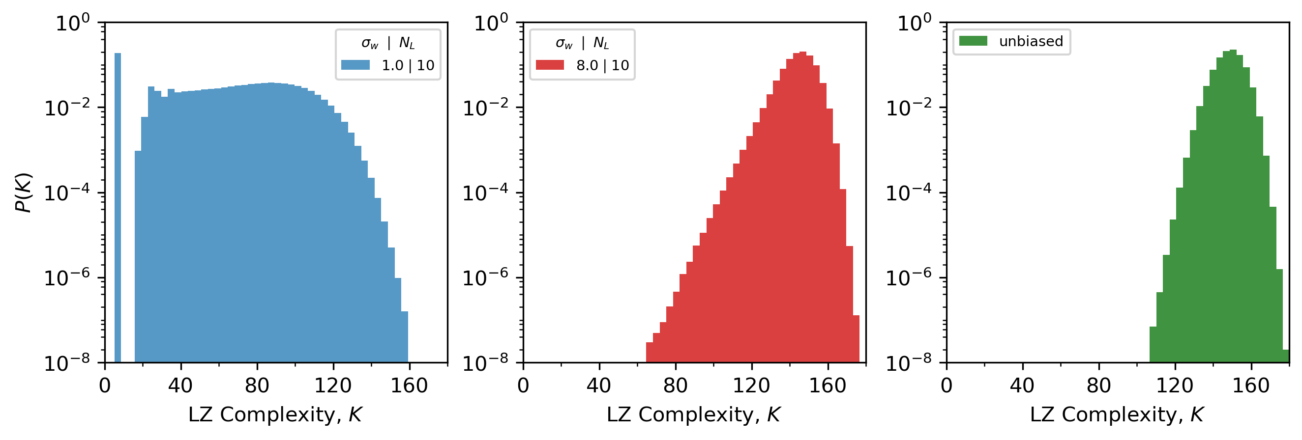

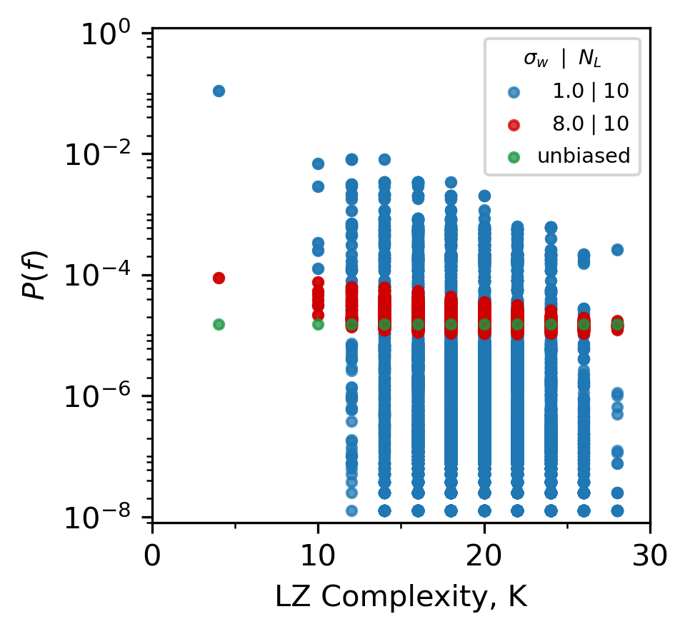
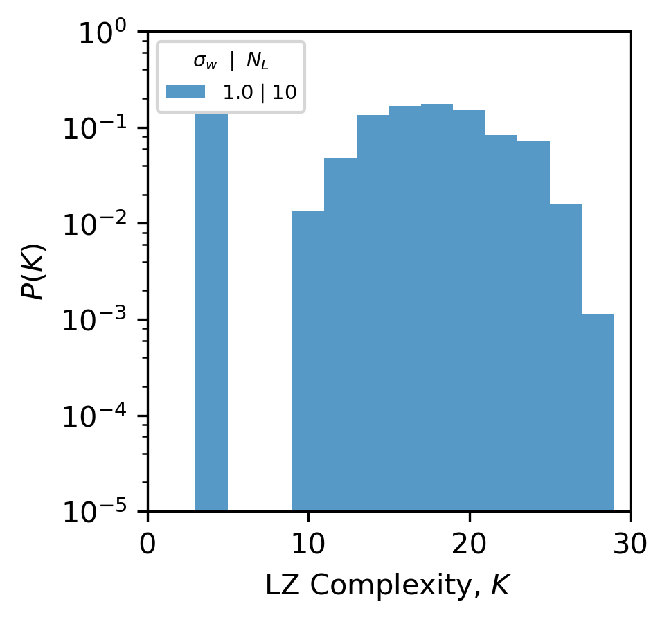
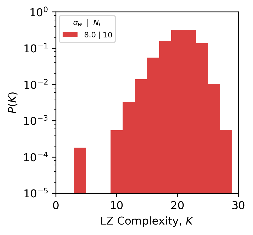
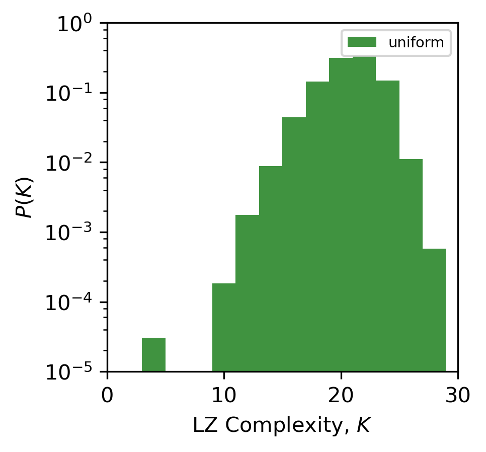
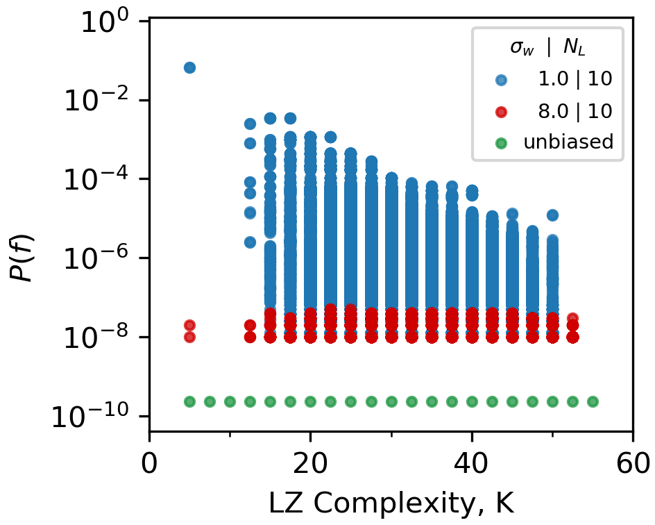
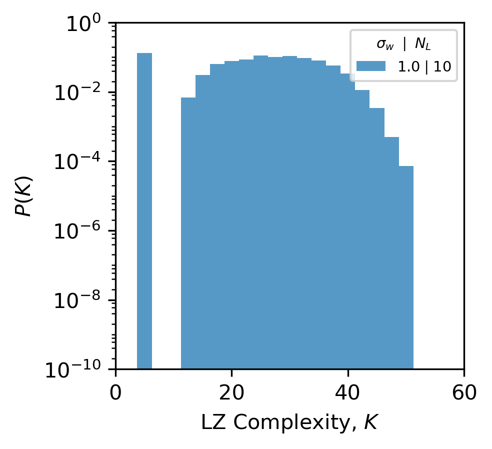
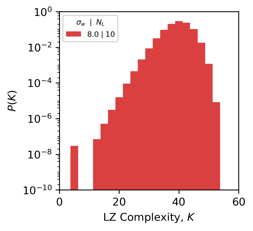
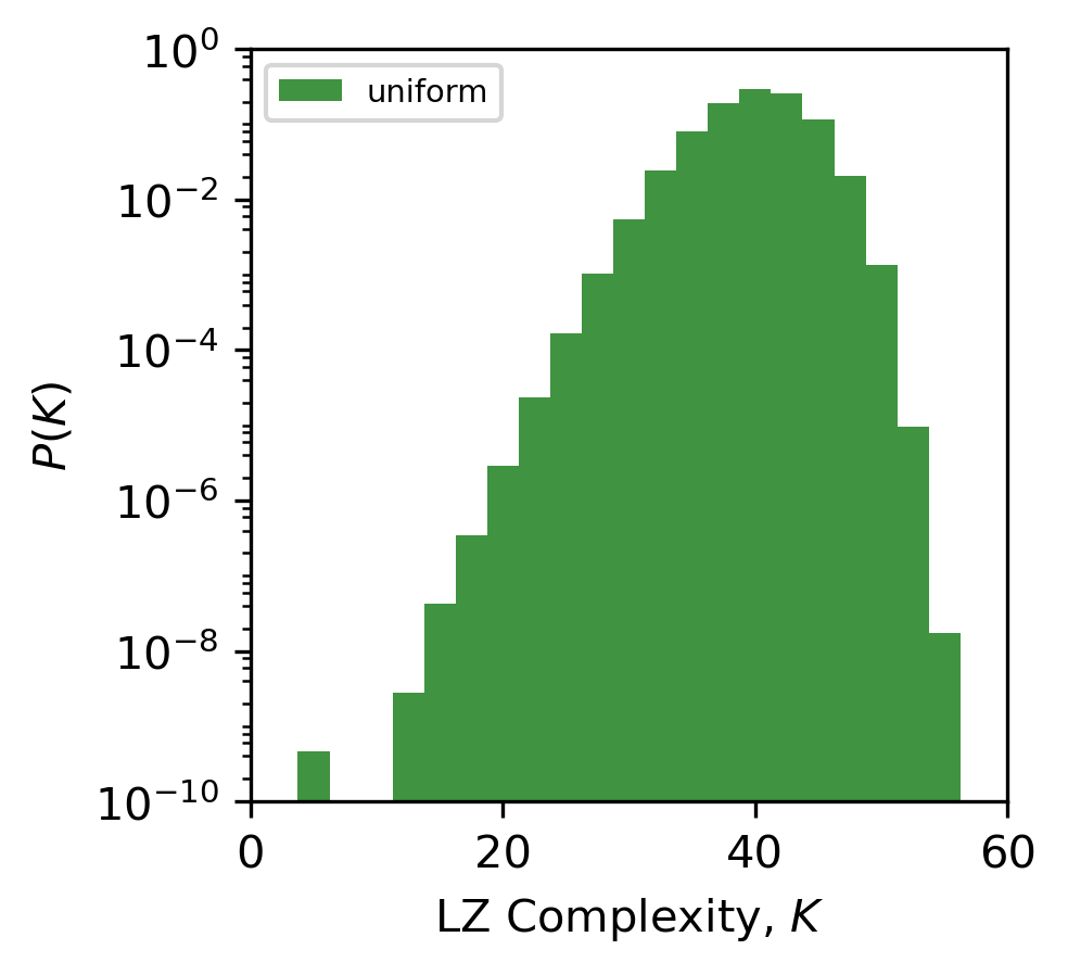
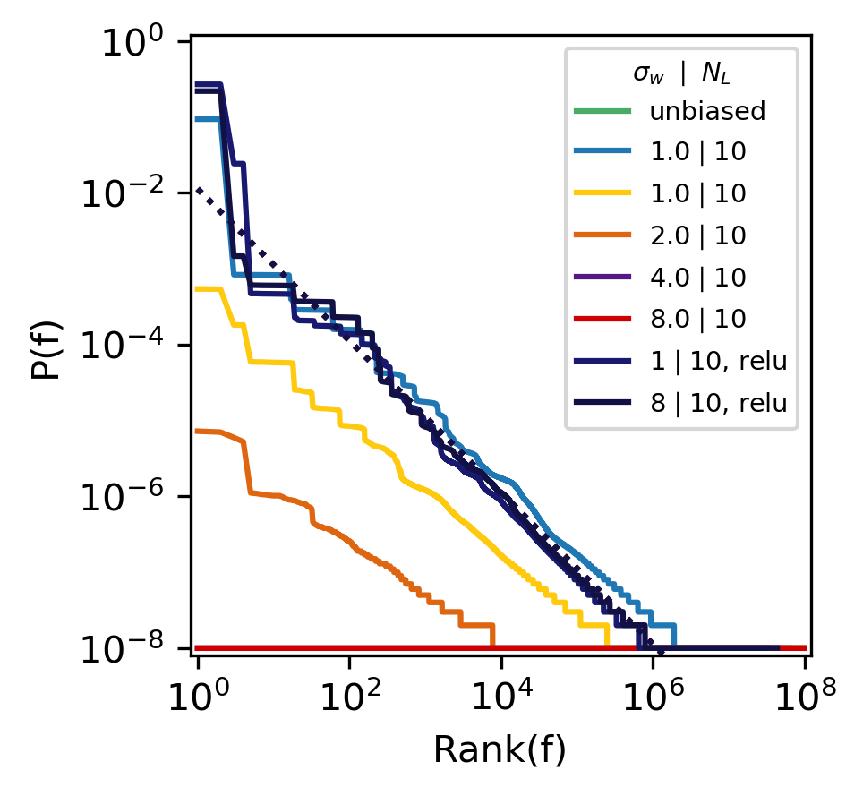
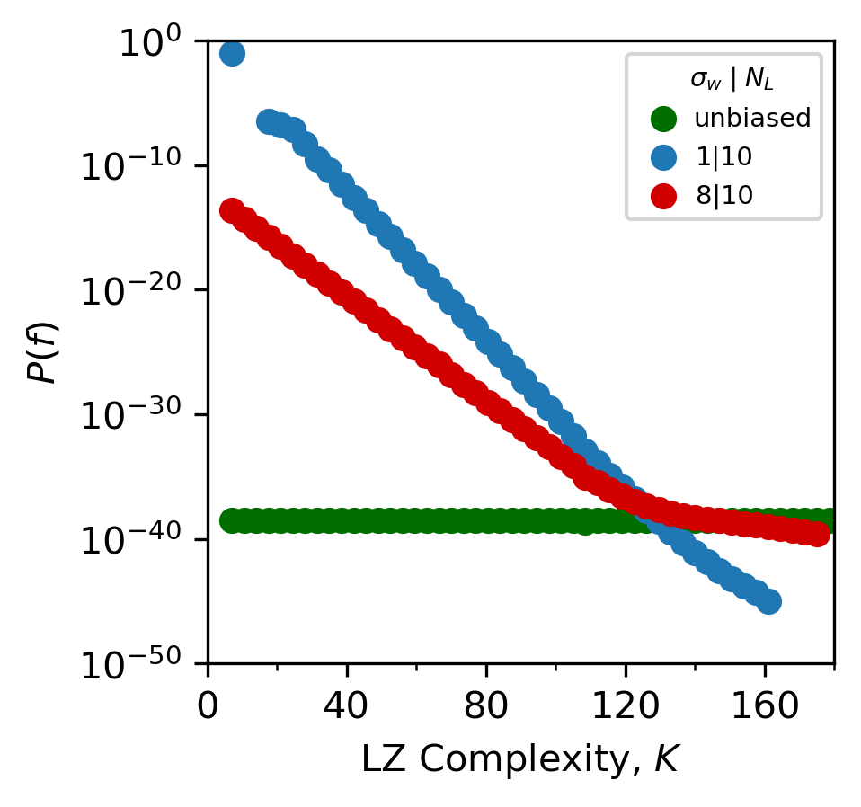
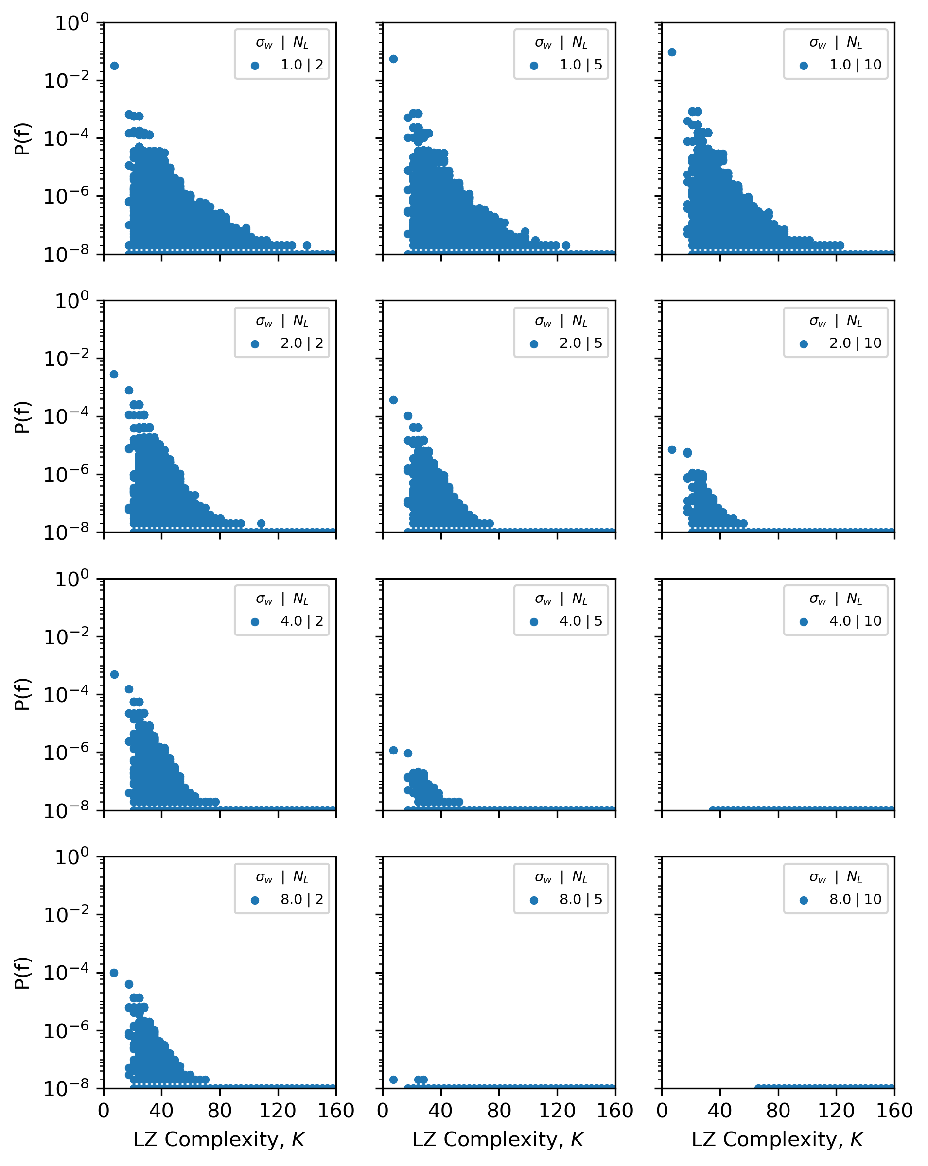
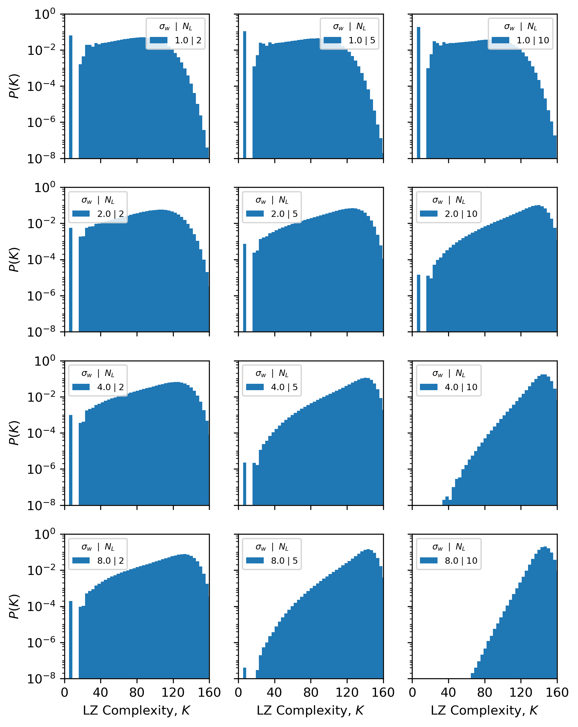
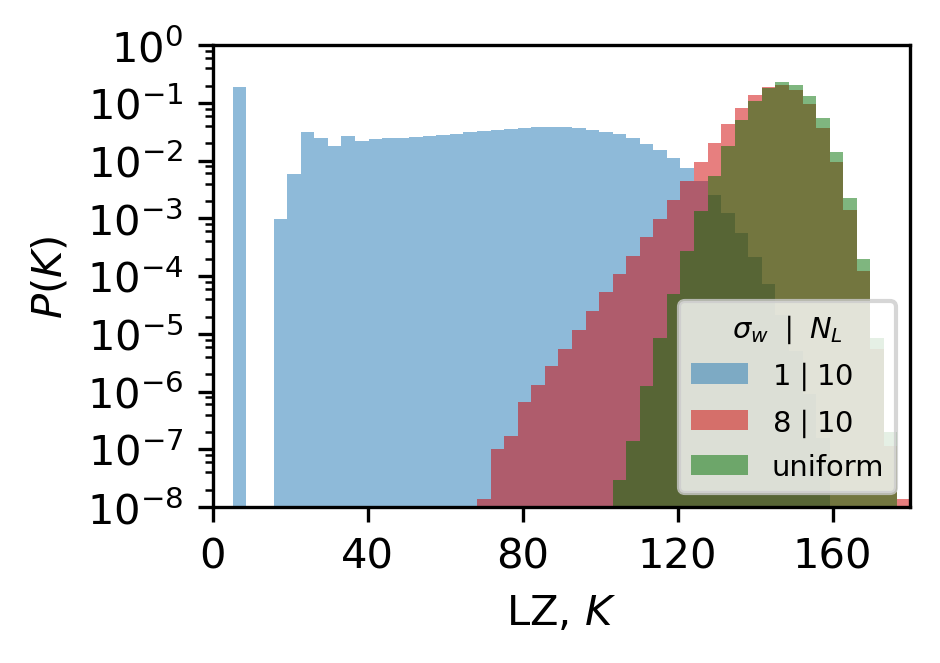
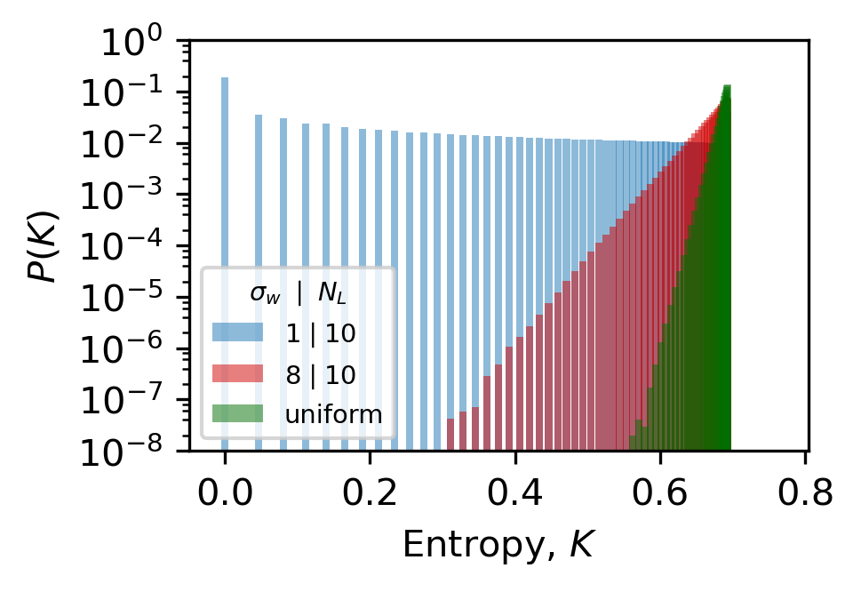
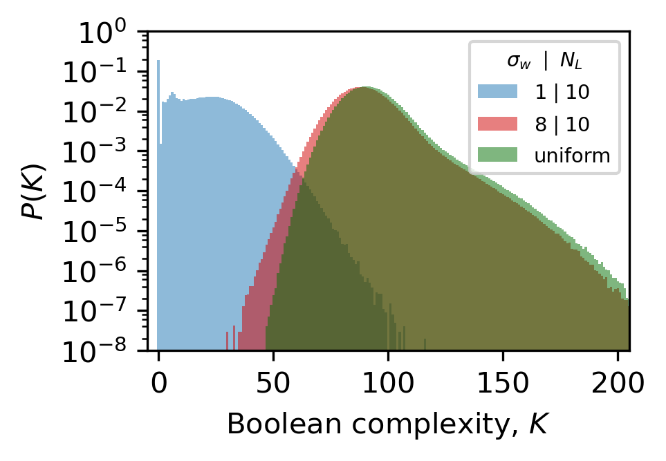
Appendix J Extended figures for generalization error, posteriors, and likelihoods
In this section, we present extended data for the generalization error with data complexity, scatter plots of error v.s. complexity, as well as the approximate average likelihoods and posteriors for the decoupling approximation, compared to posteriors from SGD. These figures complement main text figures 1 2.
In Figure S6 we display the generalization error for DNNs with different and . This figure extends Figure 1(c) in the main text. By comparing to Figure S4, one can see how the change in bias strongly affects the generalization error.
In Figure S7 and Figure S8, we show scatter plots that complement the main text scatter plots Figures 1(d), 1(e) and 1(f).
In Figure S9 we show the approximations to the posterior via the decoupling approximation Equation 3 for a wider range of complexities than shown in Figure 2. Similarly, in Figure S10 and Figure S11 we complement Figure 2 by showing the results of the decoupling approximation for and functions (respectively), chosen to calculate the mean likelihood. Note that while the decoupling approximation provides an estimate that should be proportional to the posterior, it likely will not lead to a correct normalisation on its own. In the plots, we normalise the posteriors separately. As can be seen in these plots, despite the rather strong approximations inherent in Equation 3, this approach turns out to be robust to changes in the number of functions used, and works for a range of data complexities and training set sizes. See also Figure S12 for similar calculations, but with MSE loss, and including a near-exact Bayesian approximation using a Gaussian Process (GP) approach. In all these cases the decoupling approximation captures key qualitative features of the posterior, providing an a-posteriori justification for its use for this system. It would be interesting to find an a-prior justification for this approximation as well.
.
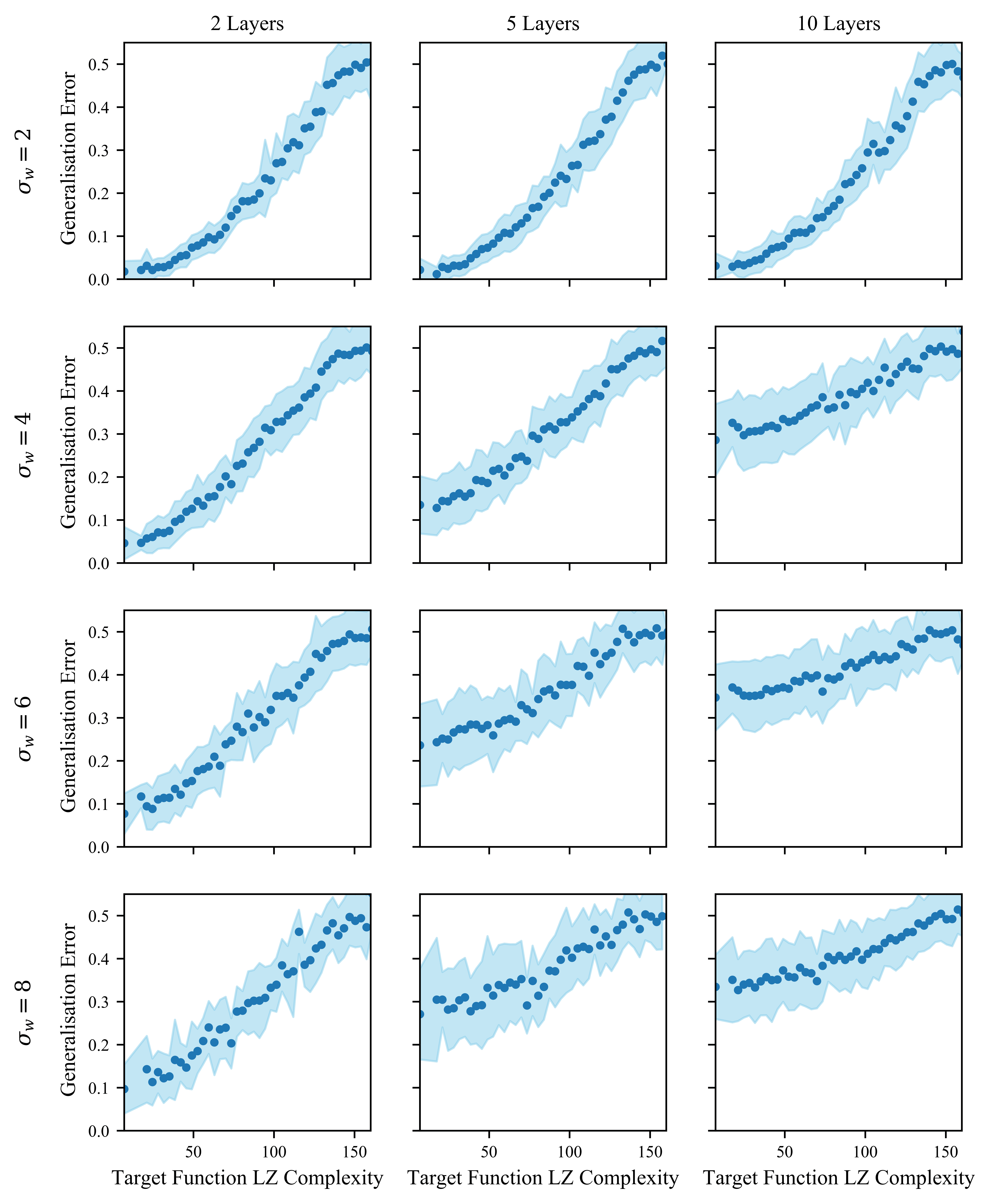
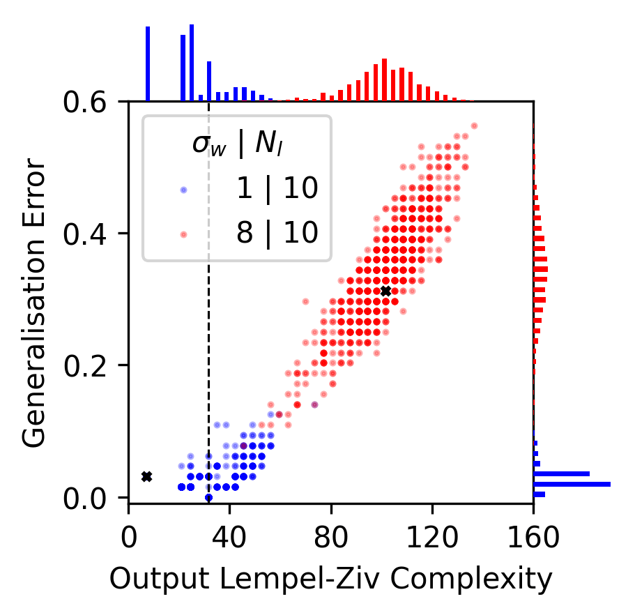
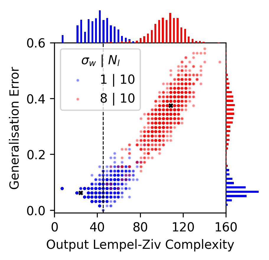
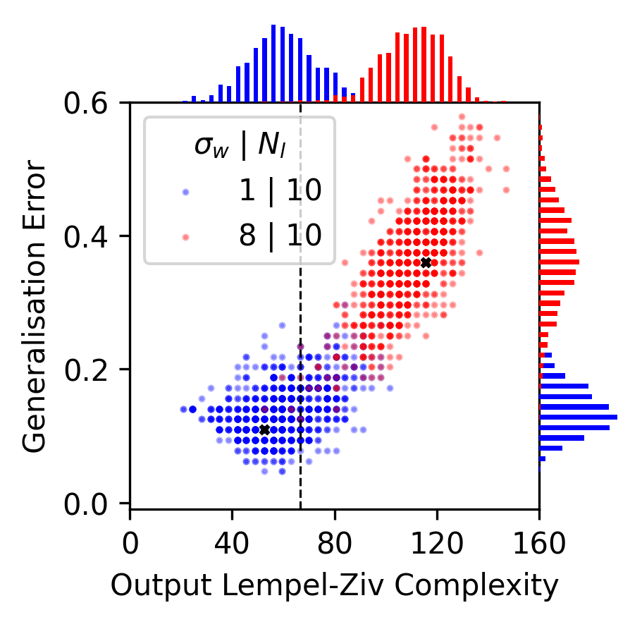
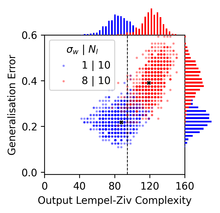
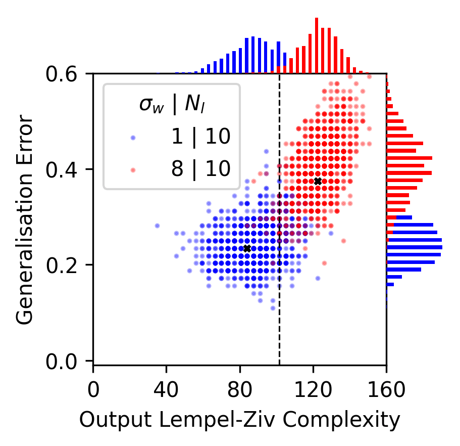
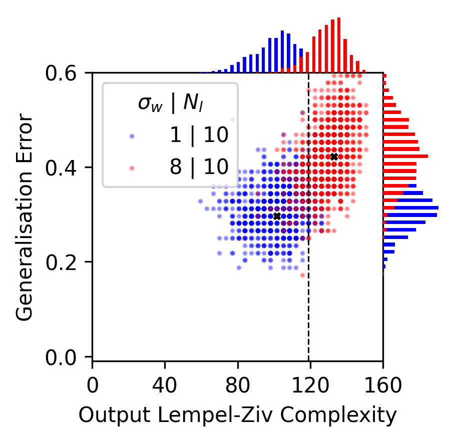
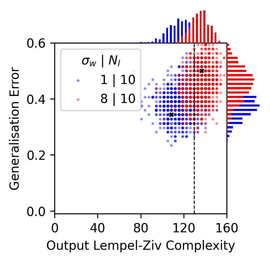
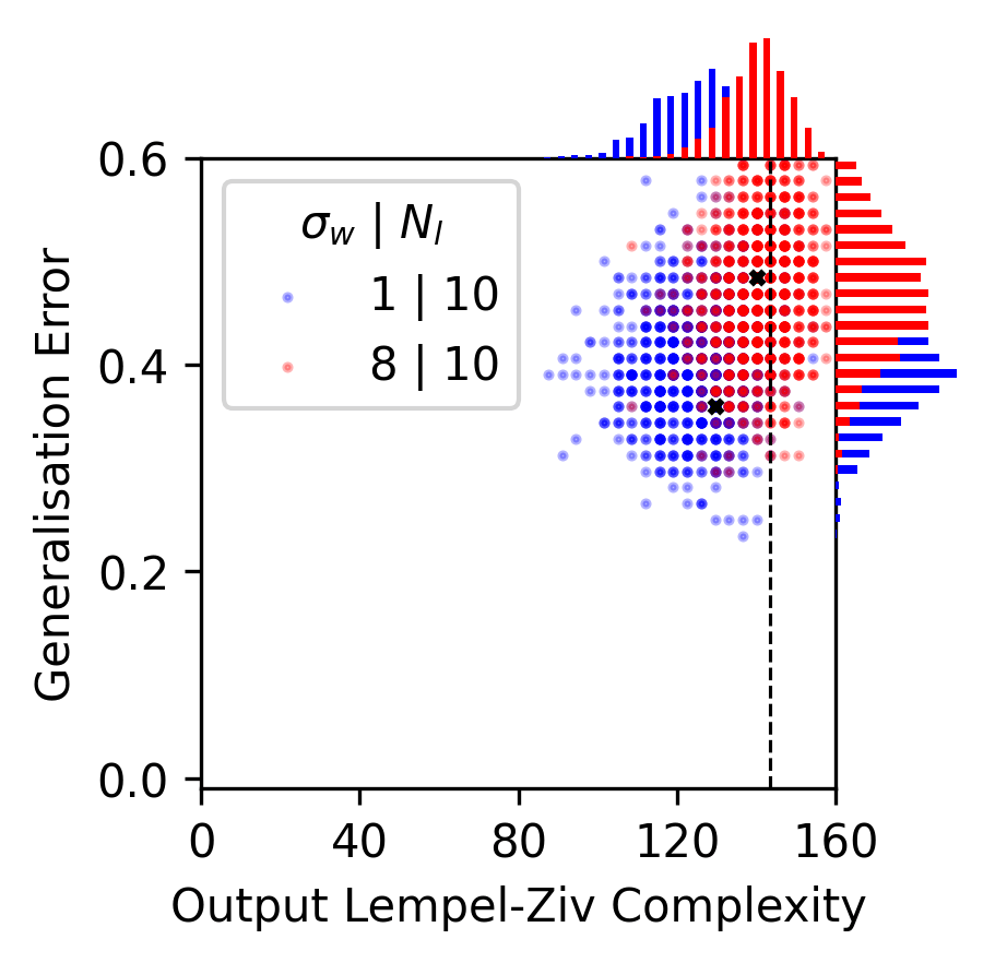


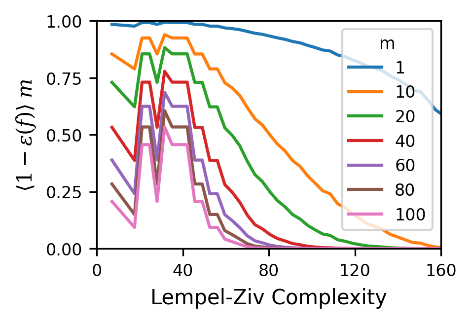
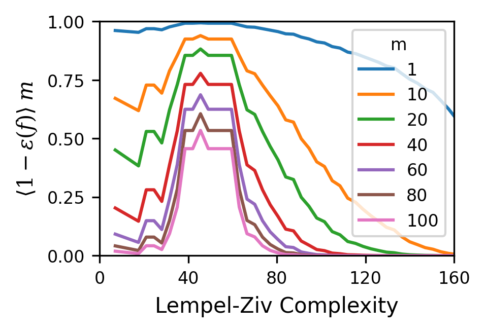
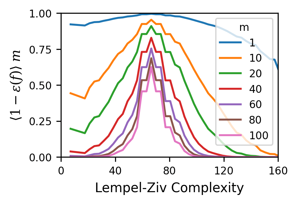
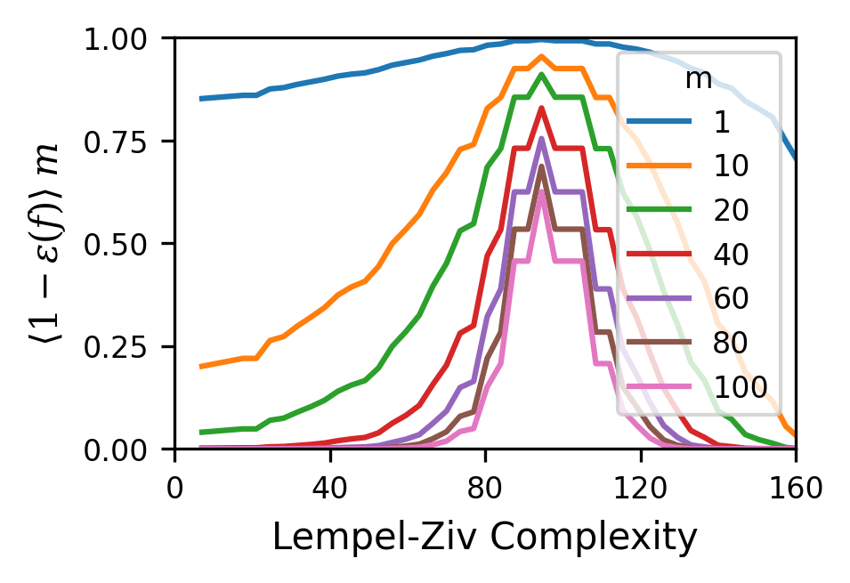
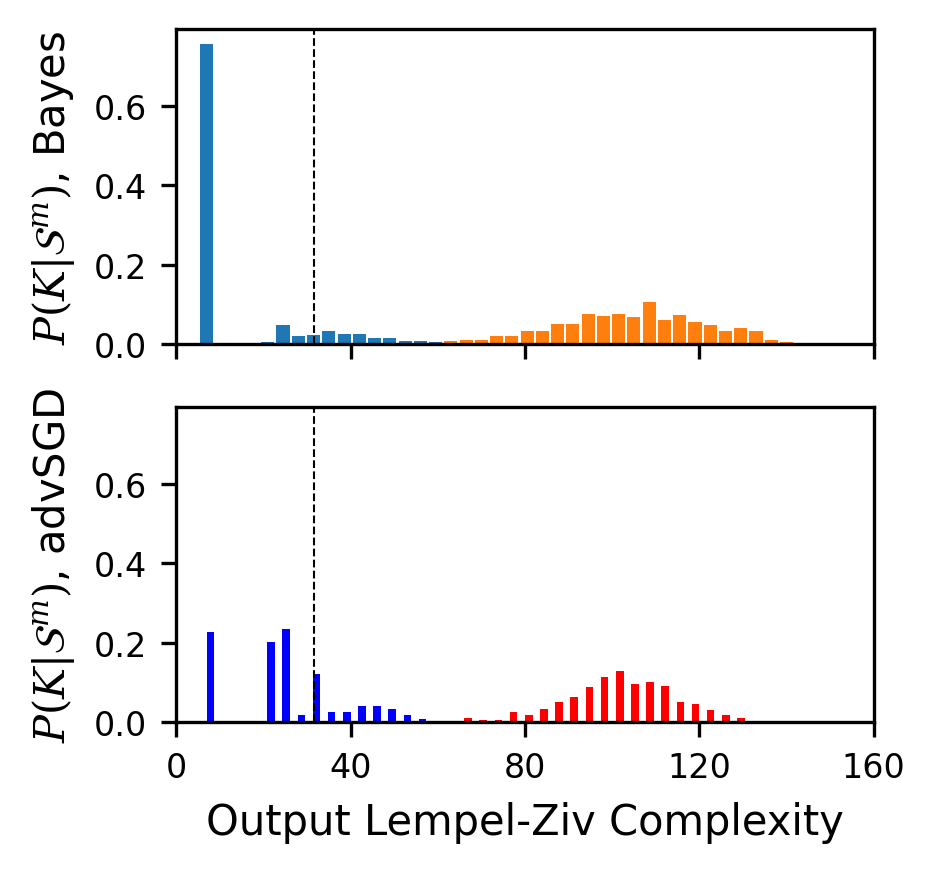
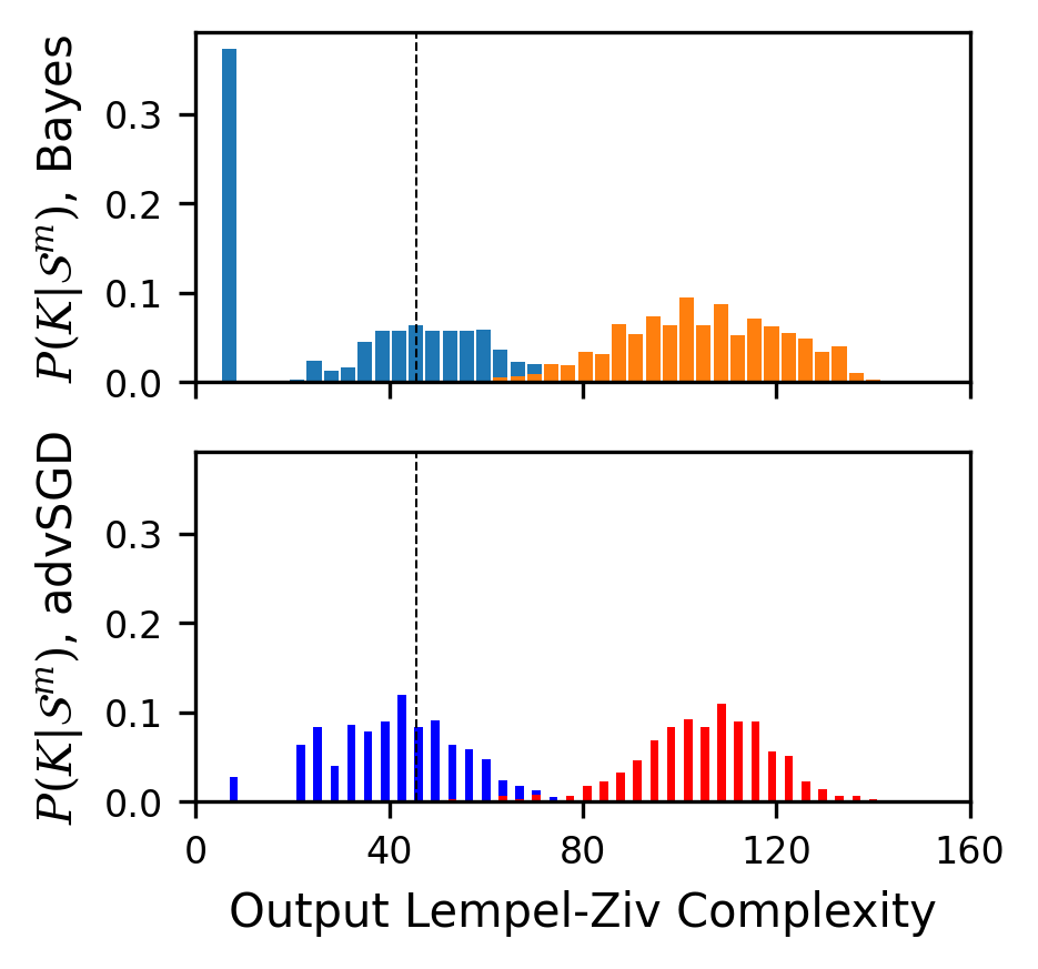
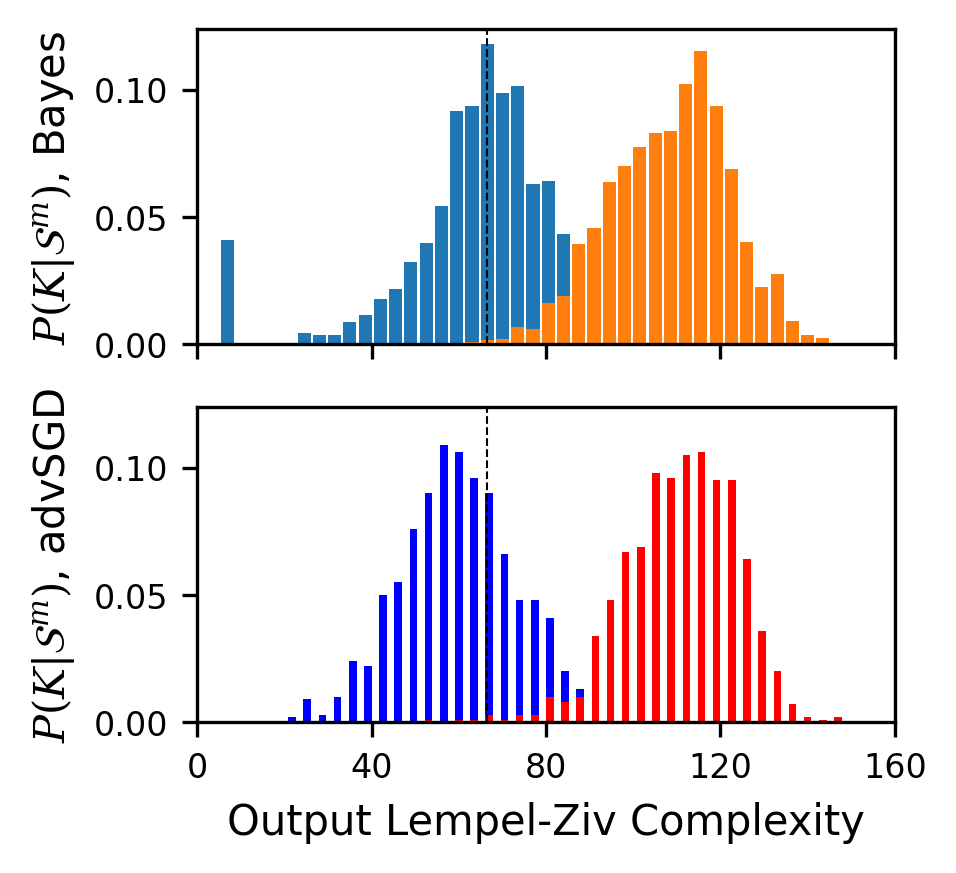
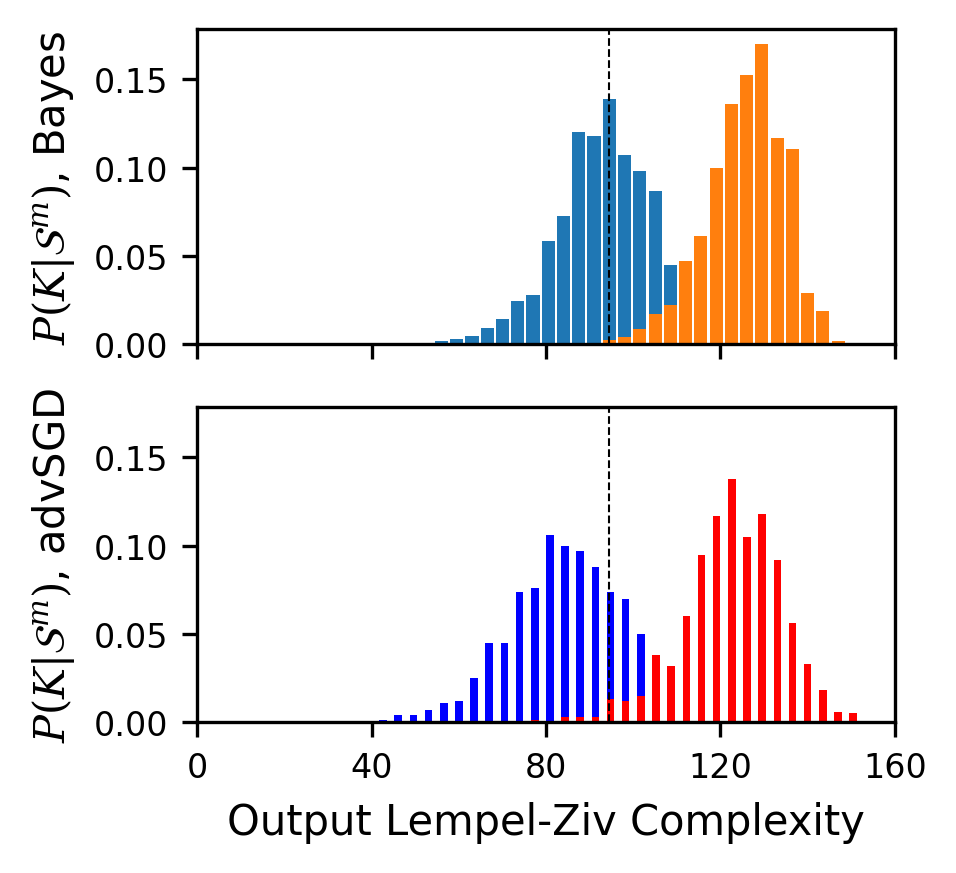
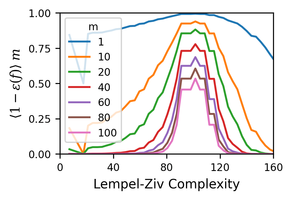
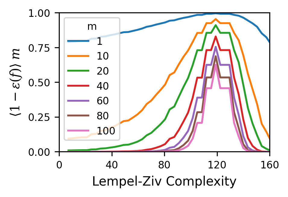
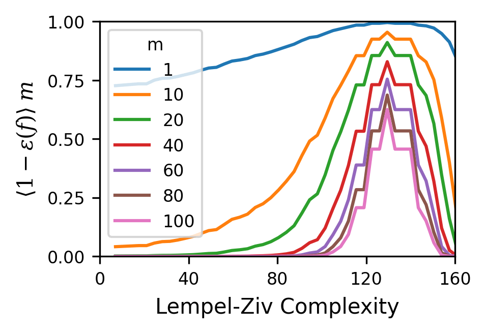
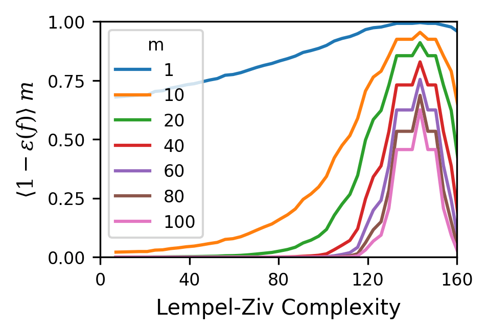
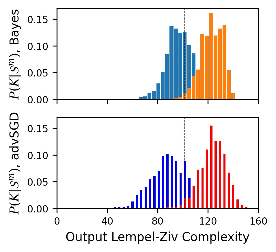
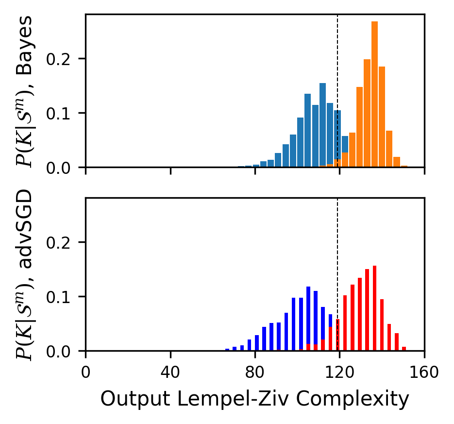
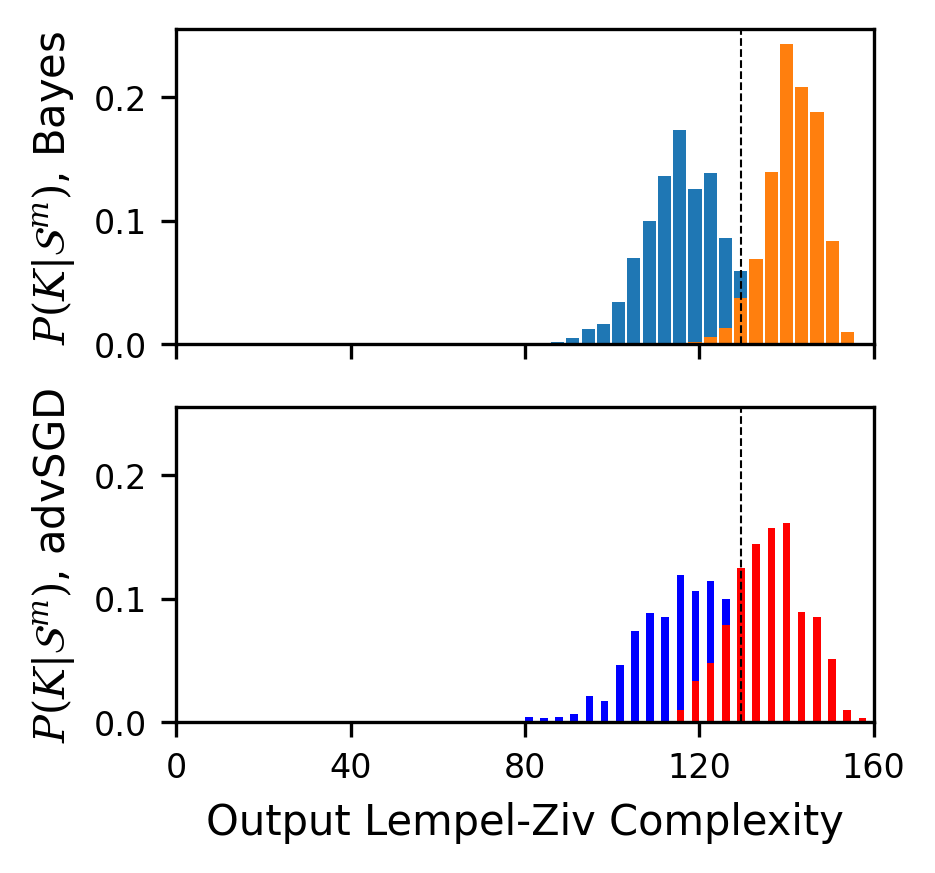
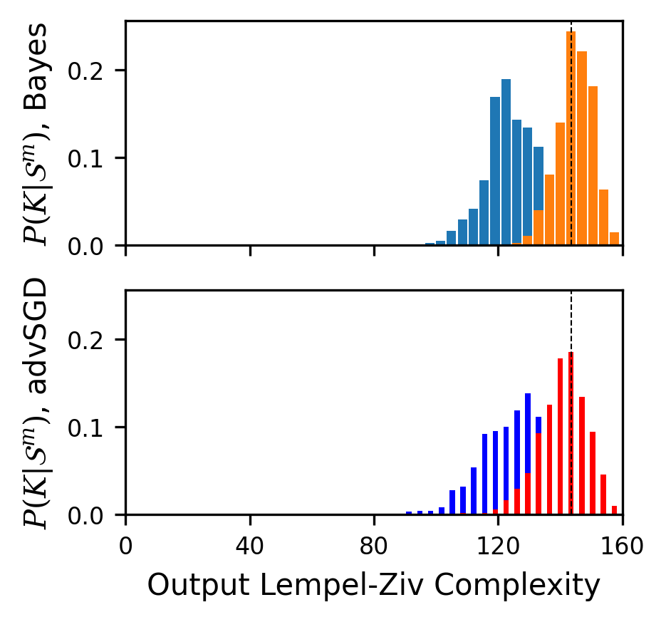
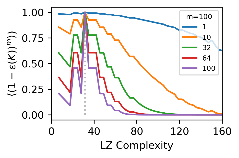
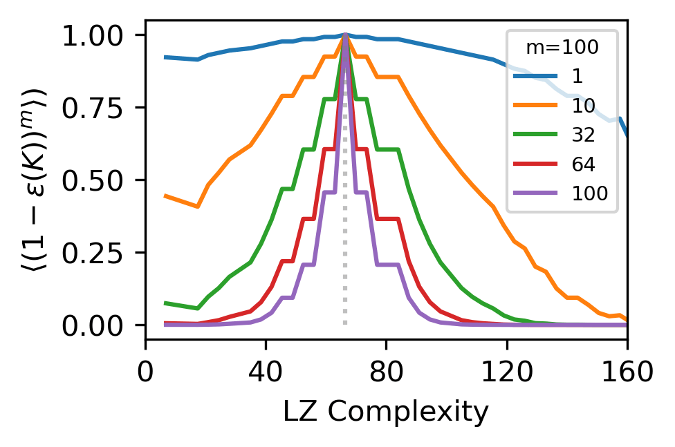
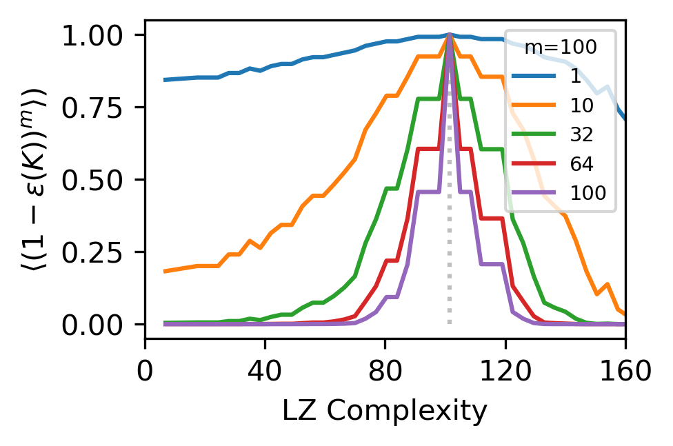
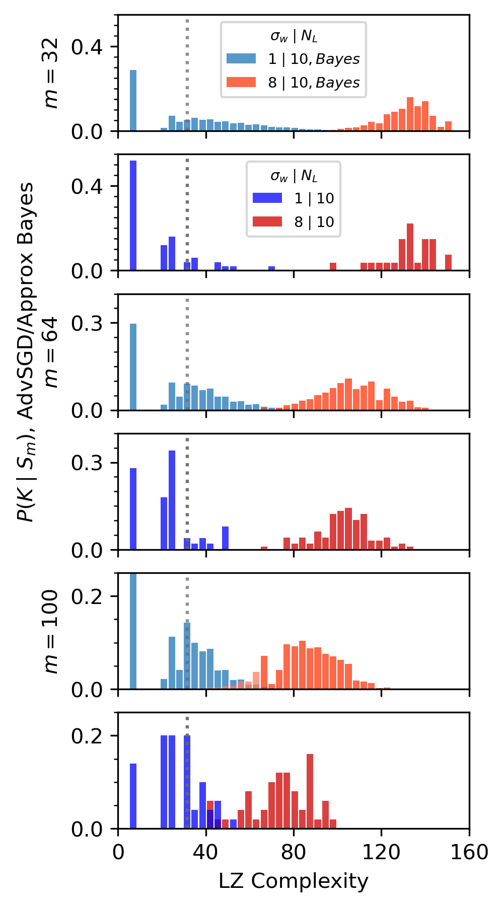
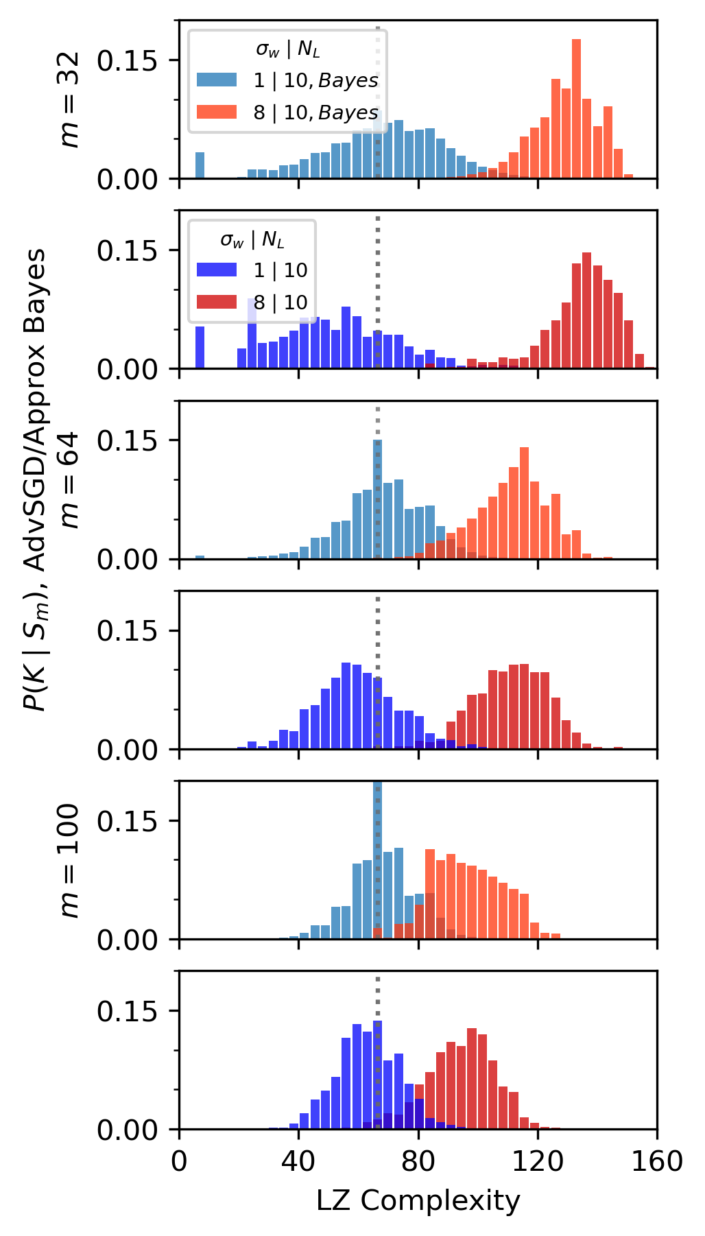
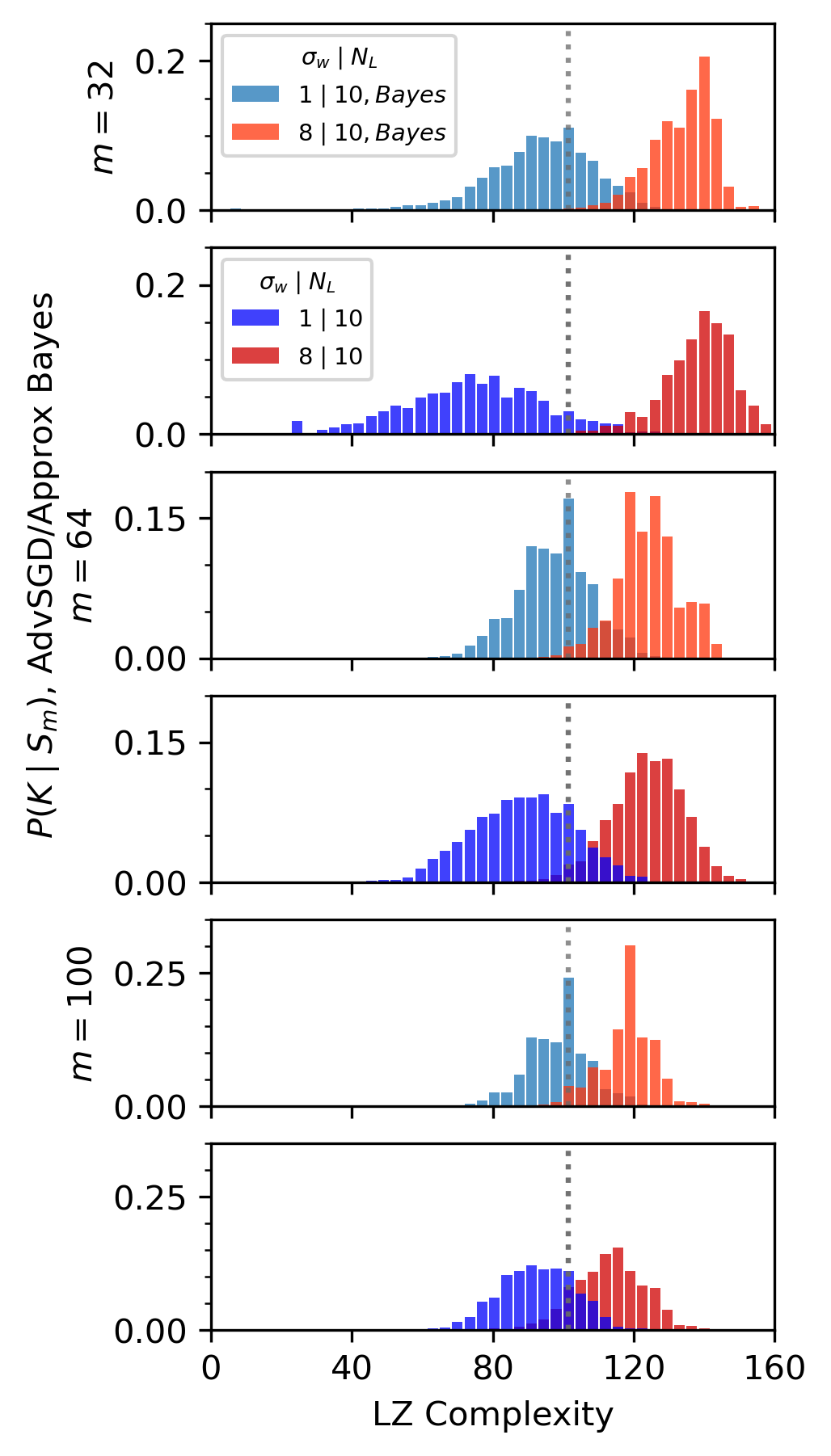
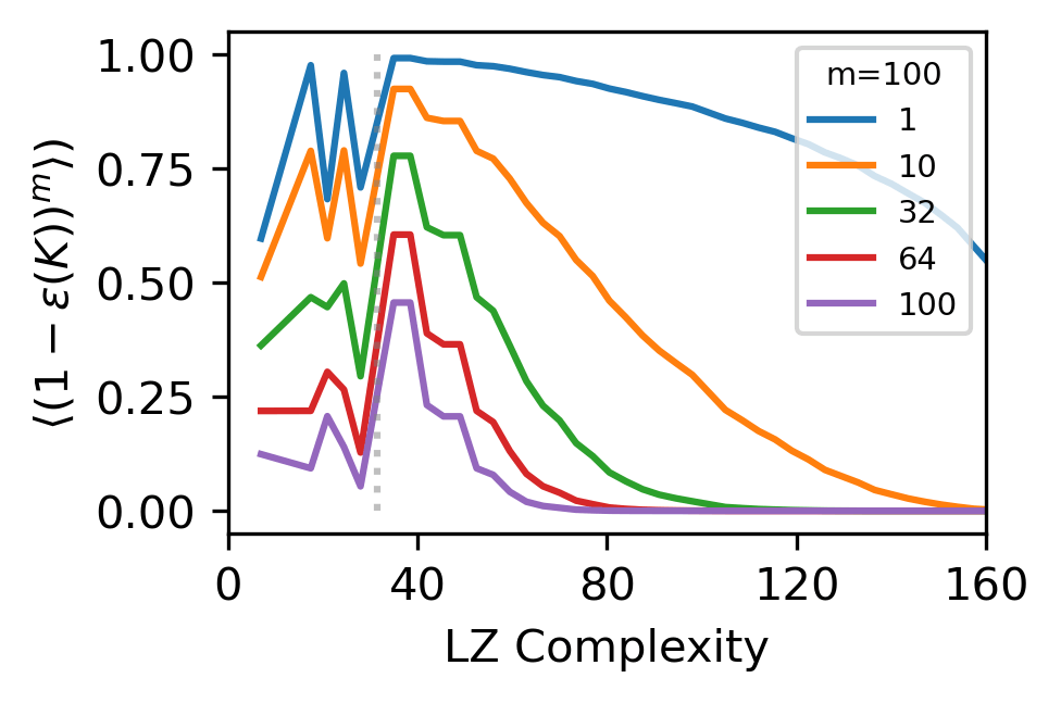
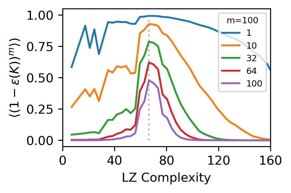
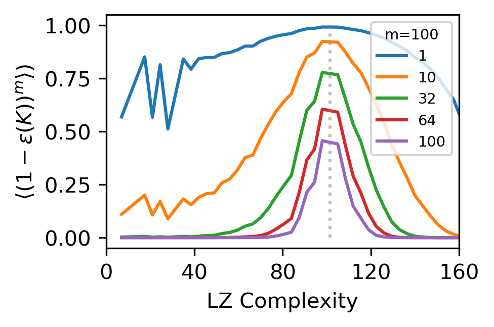
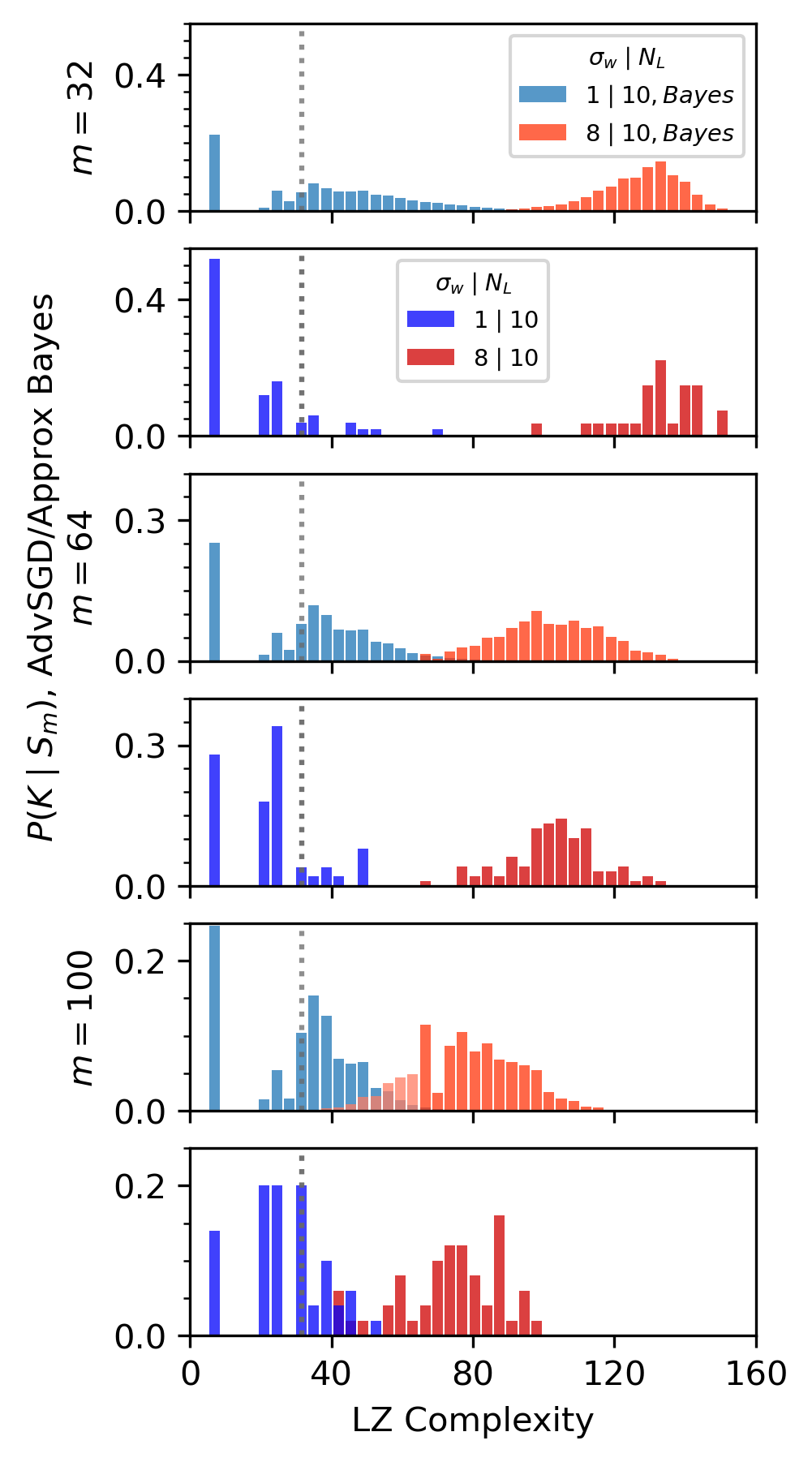
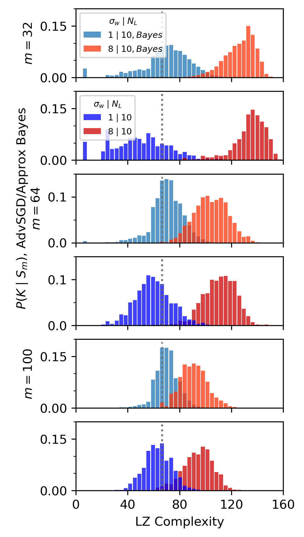
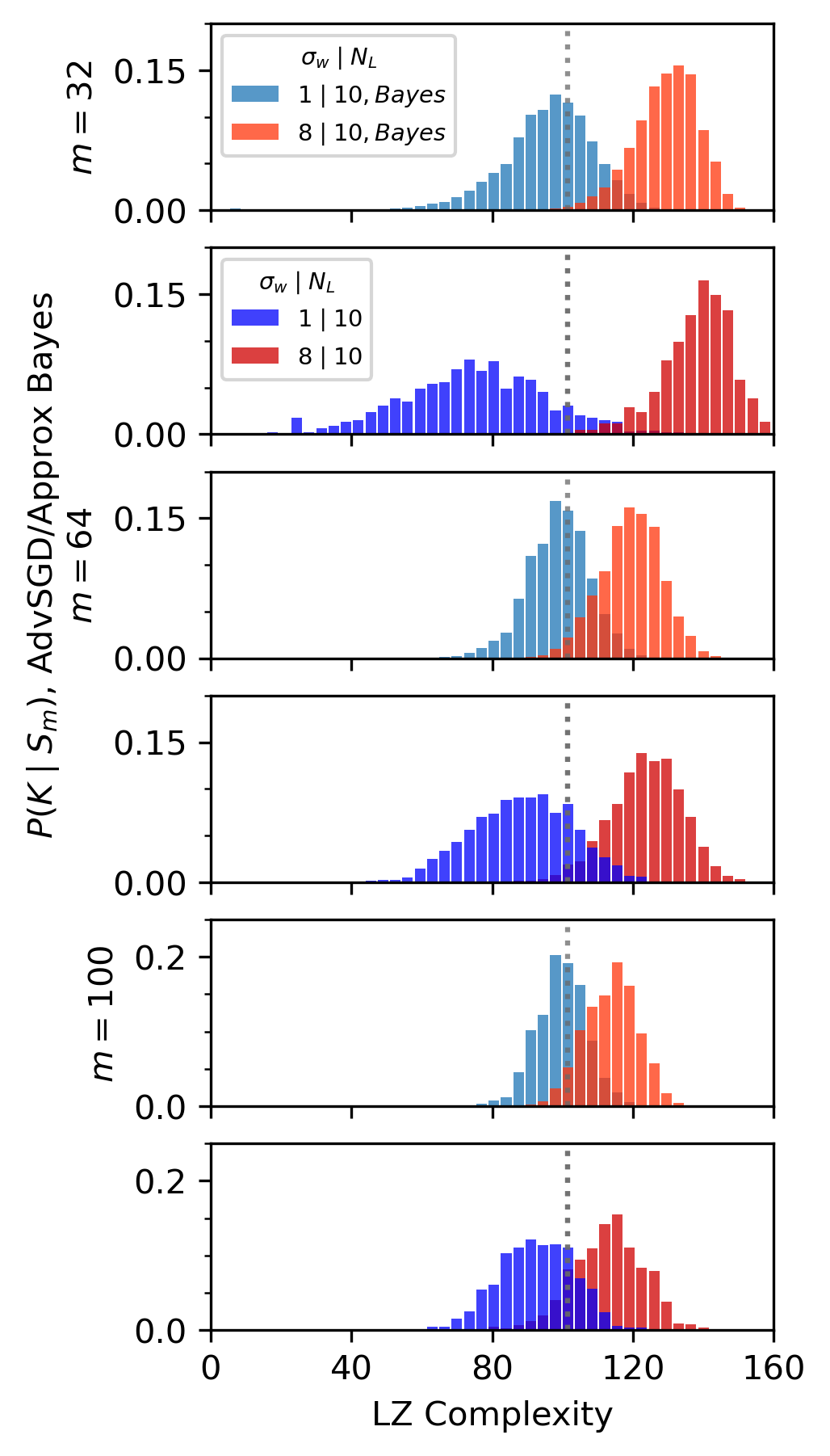
Appendix K Extended figures for generalization errors, posteriors and likelihoods for MSE loss
It is interesting to ask the question of whether or not DNNs with cross-entropy (CE) loss behave fundamentally differently than those using MSE loss. In this section, we repeat some of the analysis from the main text for MSE loss. An advantage is that we can easily calculate Bayesian posteriors using a GP approach on extremely wide networks, showing that , where is the fully Bayesian posterior.
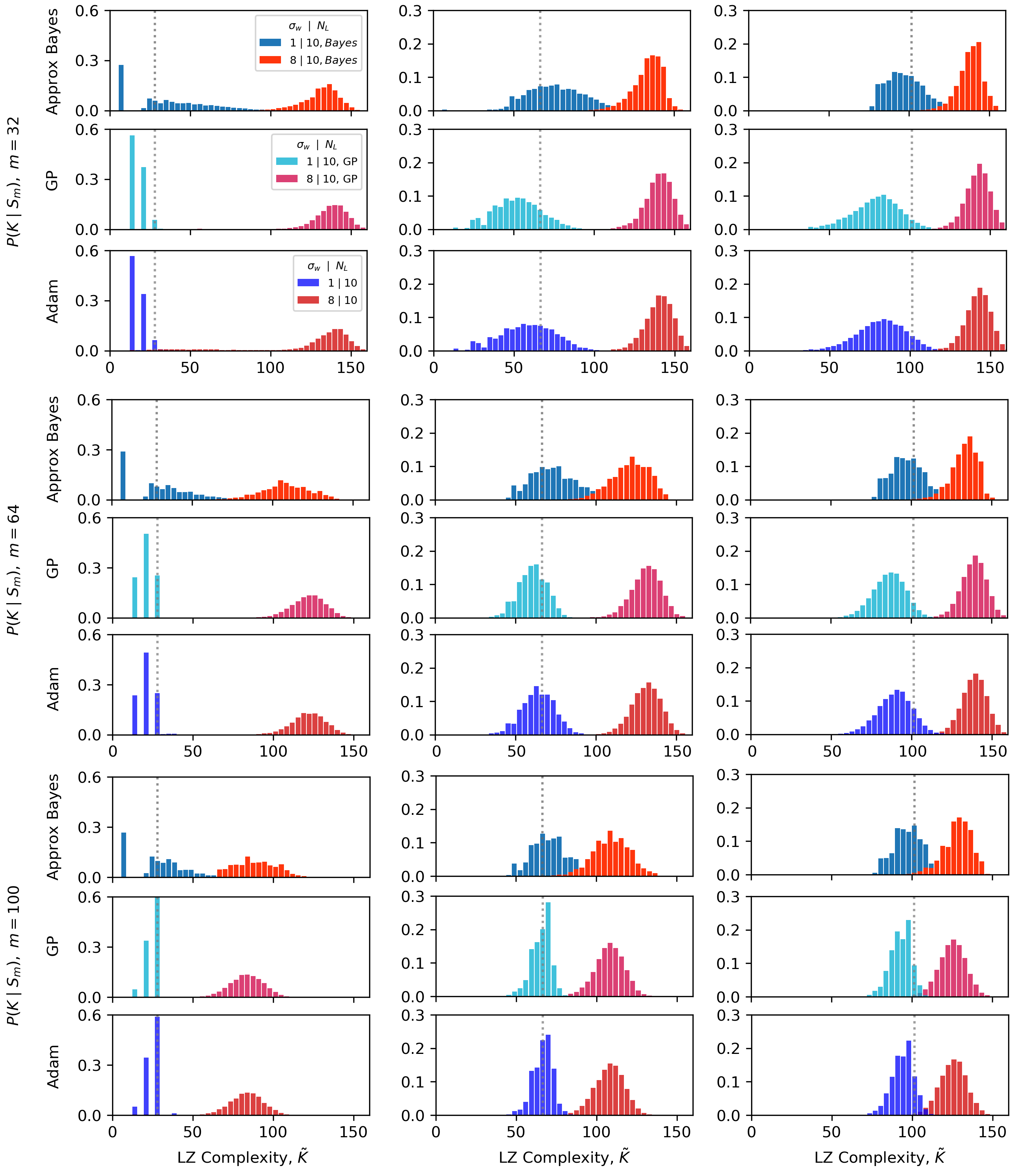
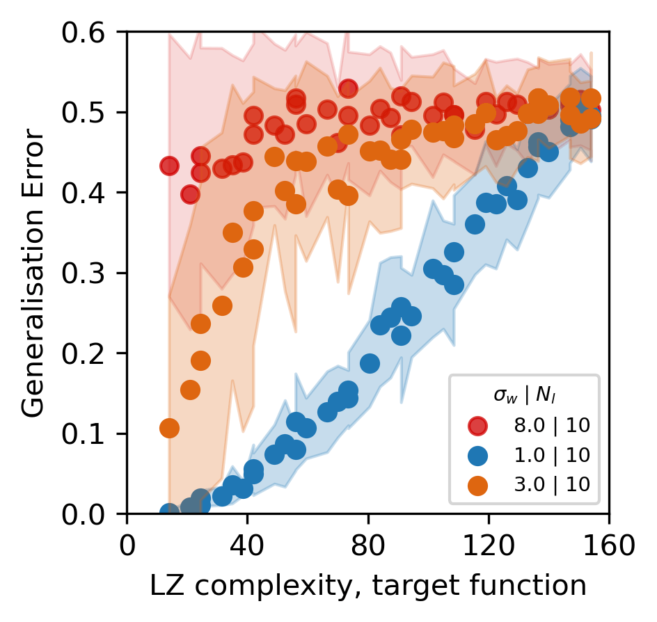
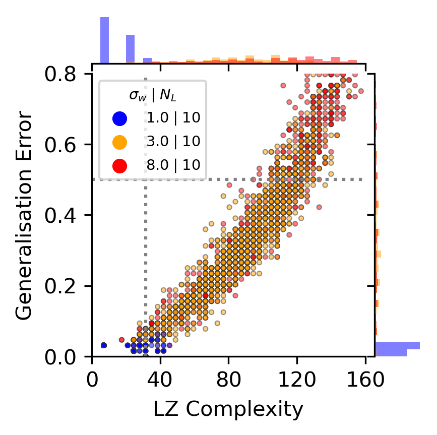
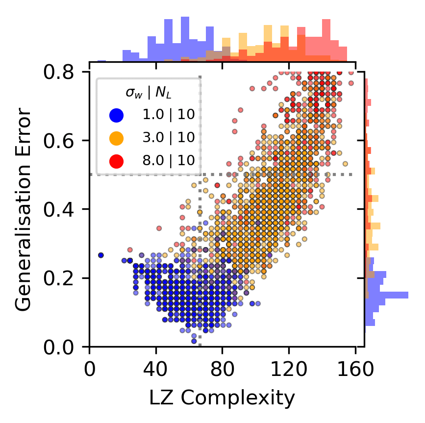
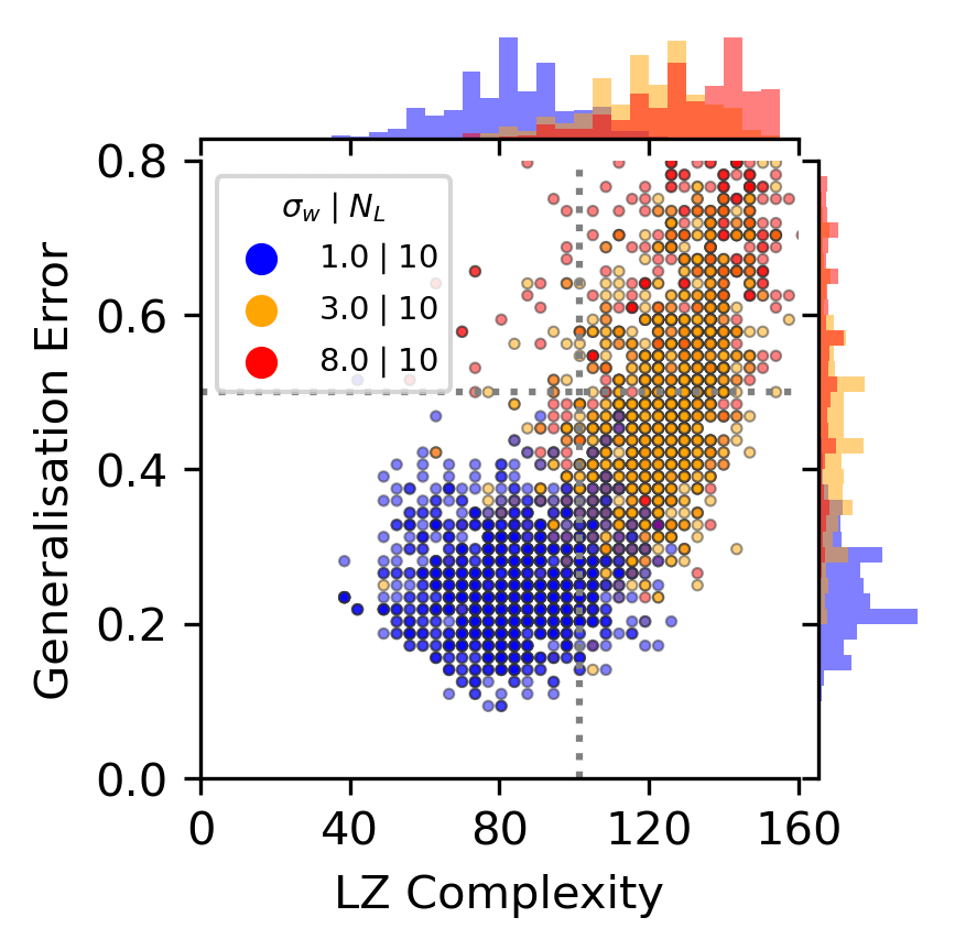
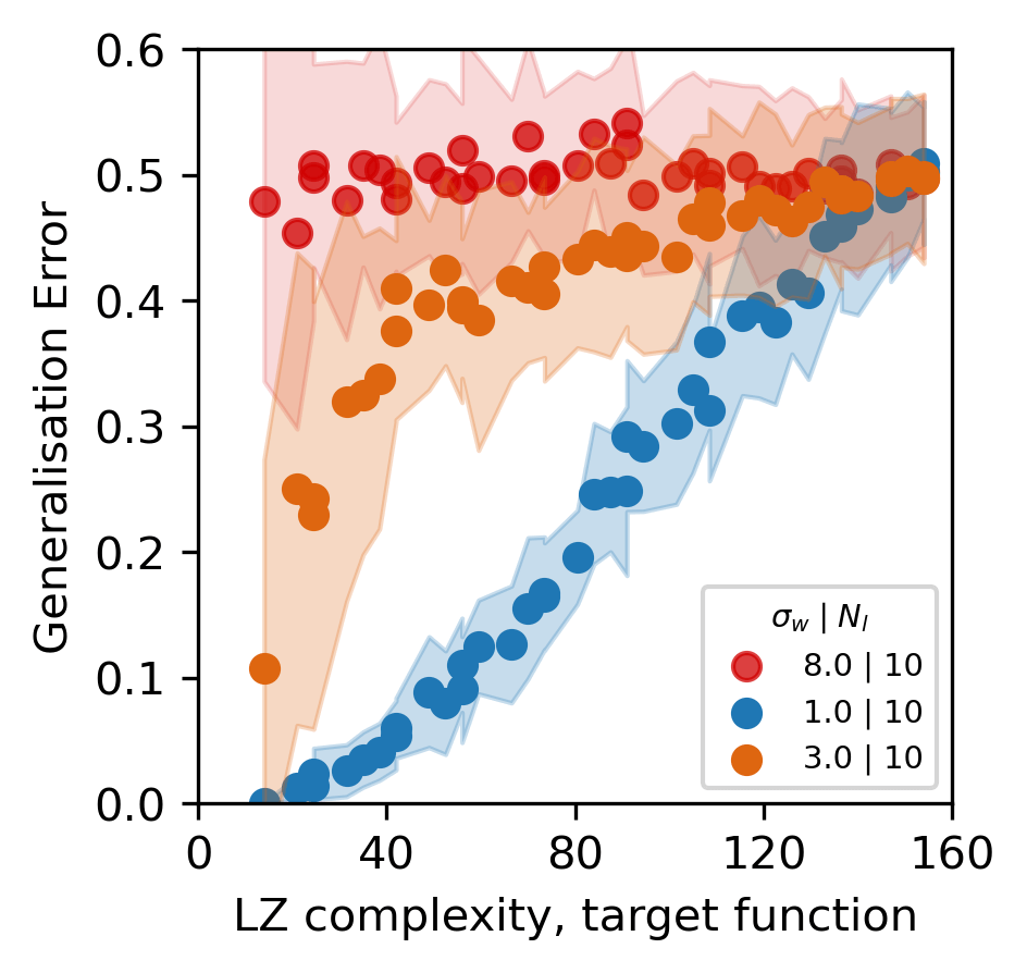
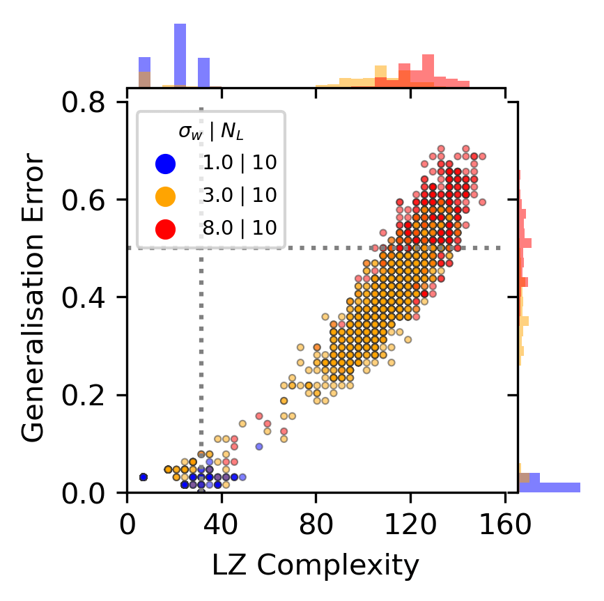
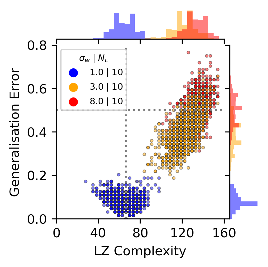
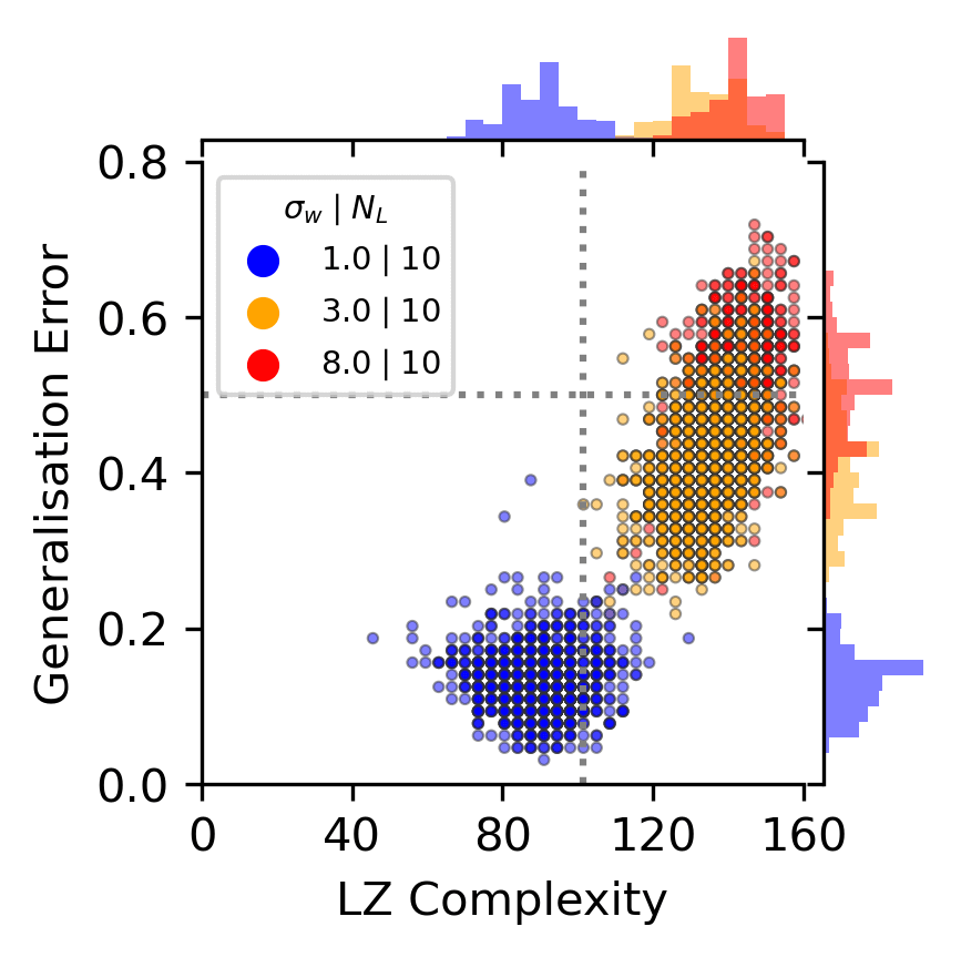
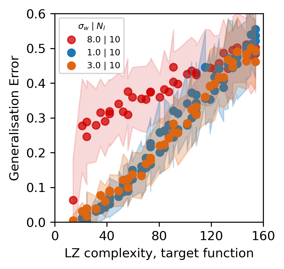
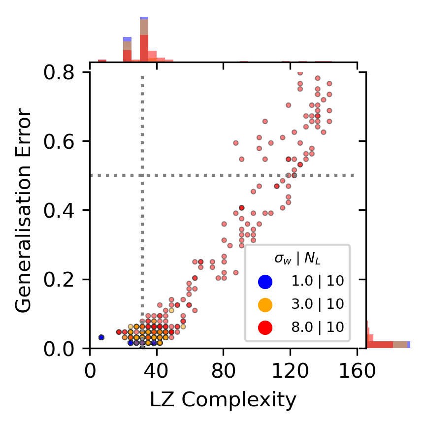
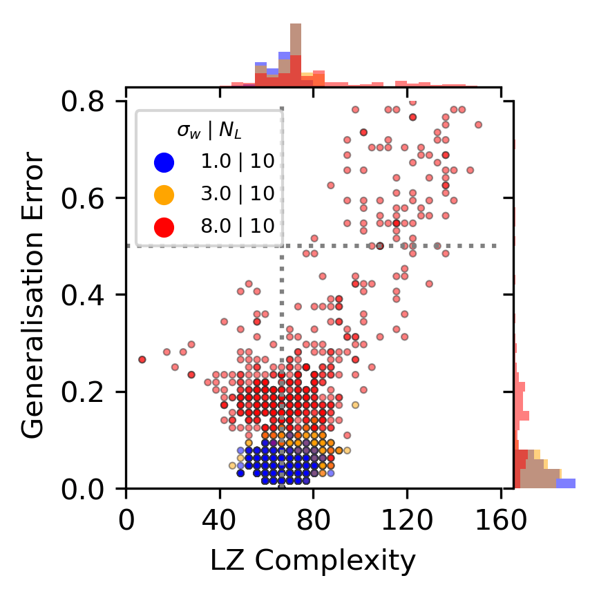
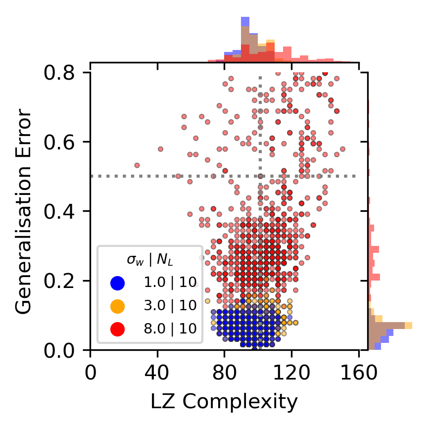
Appendix L Extended data for MNIST and CIFAR datasets and CSR complexity
In this section, we show extended data for Figure 3, where we plot generalization errors, priors, and scatterplots for MNIST and CIFAR10 datasets.
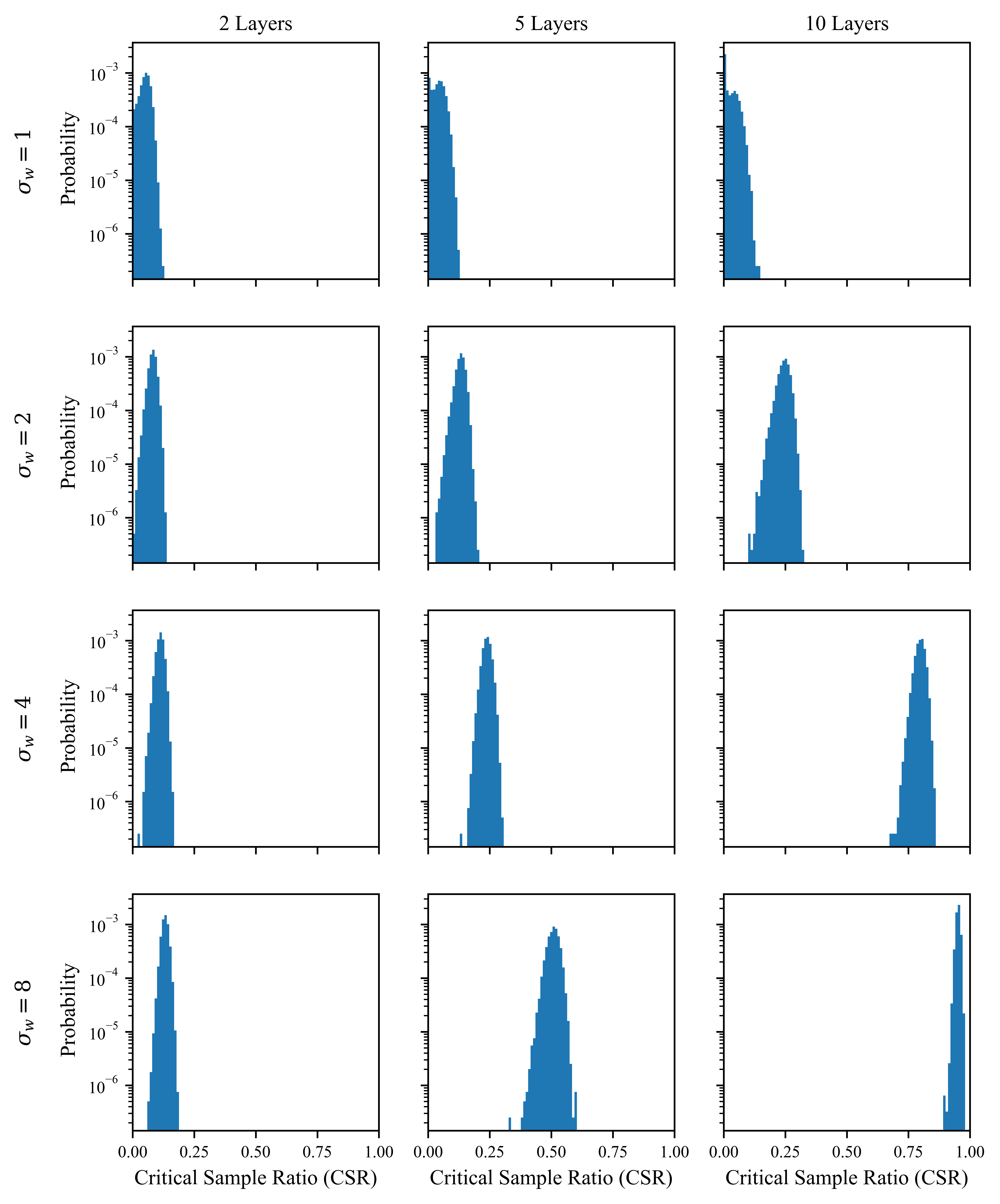
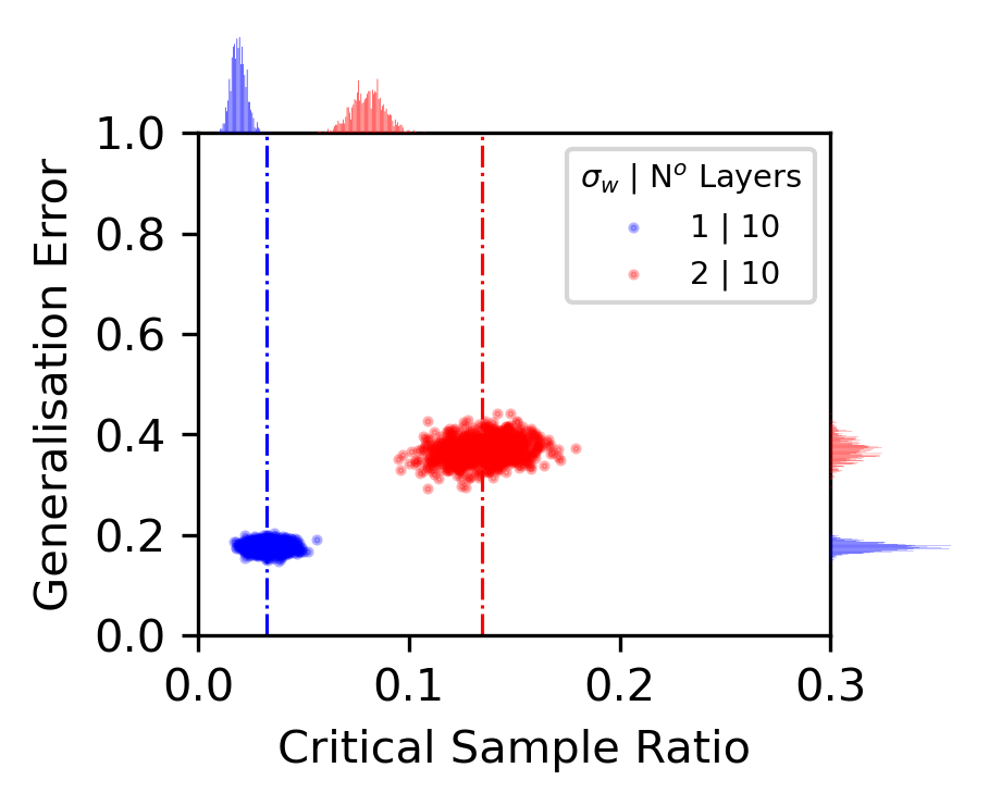
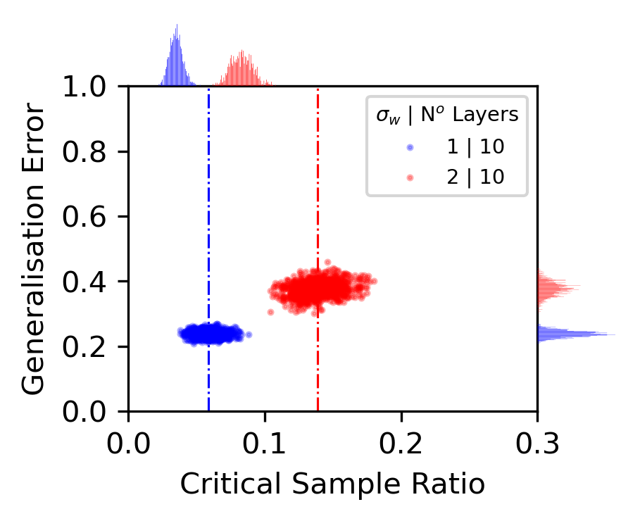
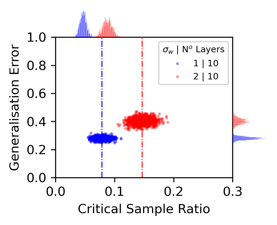
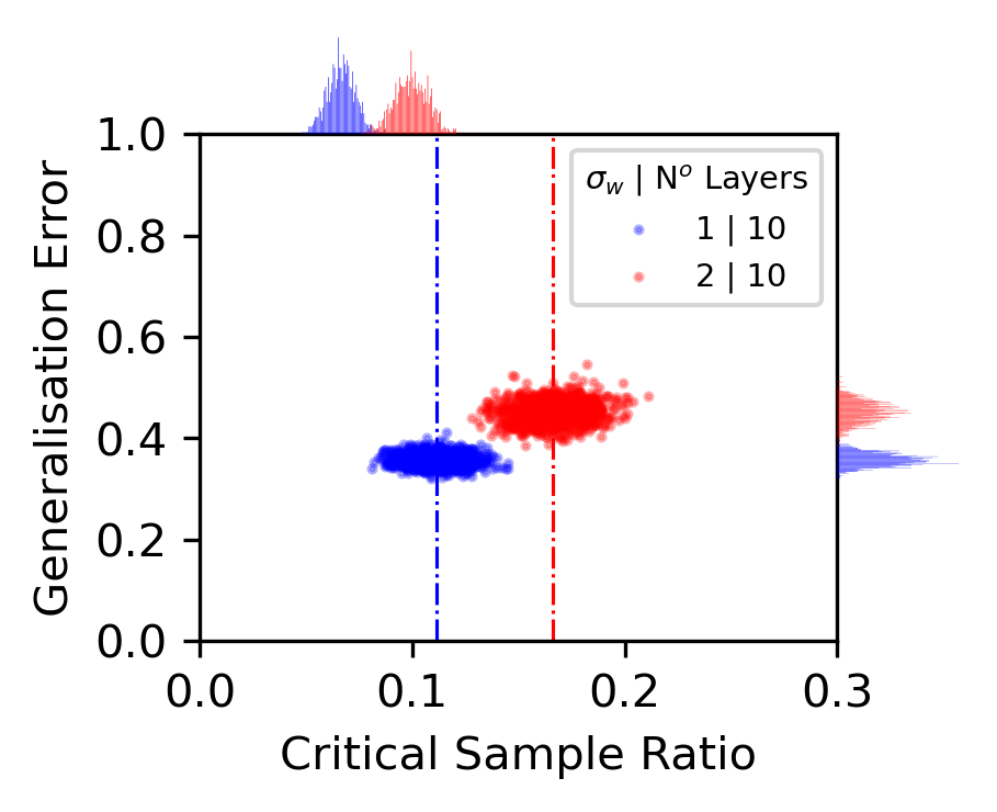
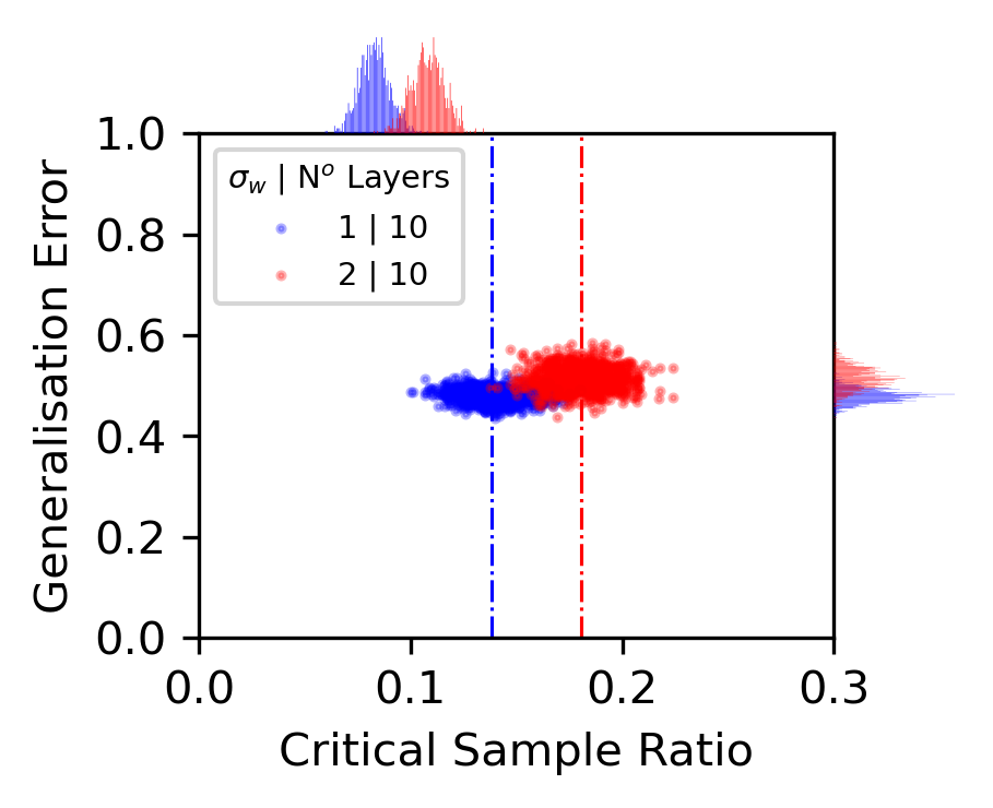
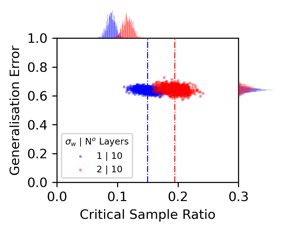
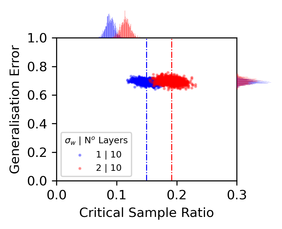
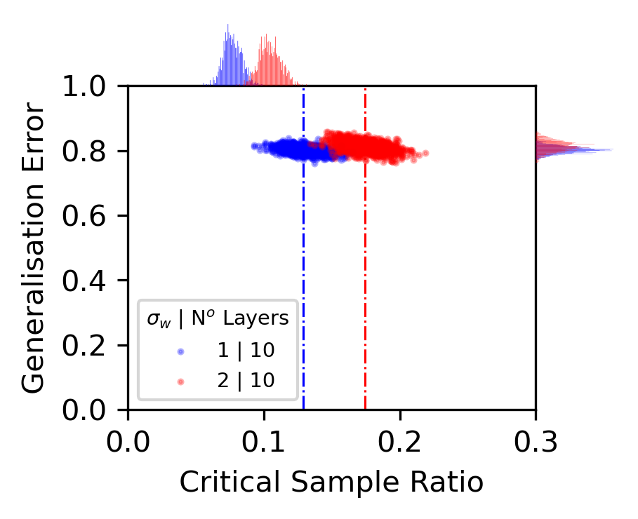
Appendix M Extended data for K-learner with PAC and PAC-Bayes bounds
In this section, we expand on Figure 1 (i) for different target functions, as well as for the smaller system. As can be seen in Figure S16 for and in Figure S17 for , there are clear differences in performance on simple rather than complex functions. We also include a lowK lowP function that is simple, but has low probability (and so is far from the bound) (see [87] for a longer discussion of such functions). We would expect (and indeed observe for ) that the DNN struggles more with functions for which it has a smaller , and therefore a smaller inductive bias at initialization. Finally, we study the parity function, for which if the number of ones in the input is even (odd). It, therefore, has the highest input sensitivity of any function, because any change of input changes the function output. There are well-known questions in the field about whether or not a DNN can learn the parity function [134, 12].
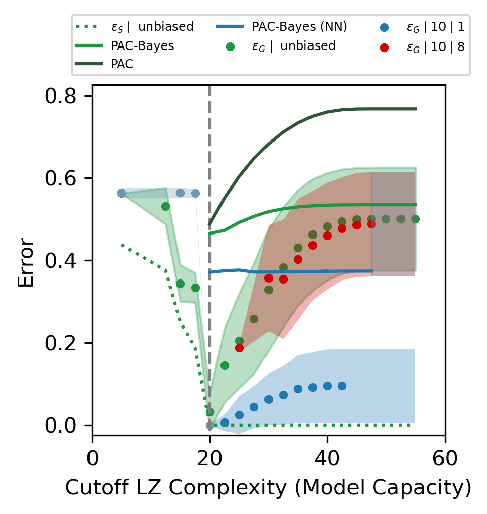
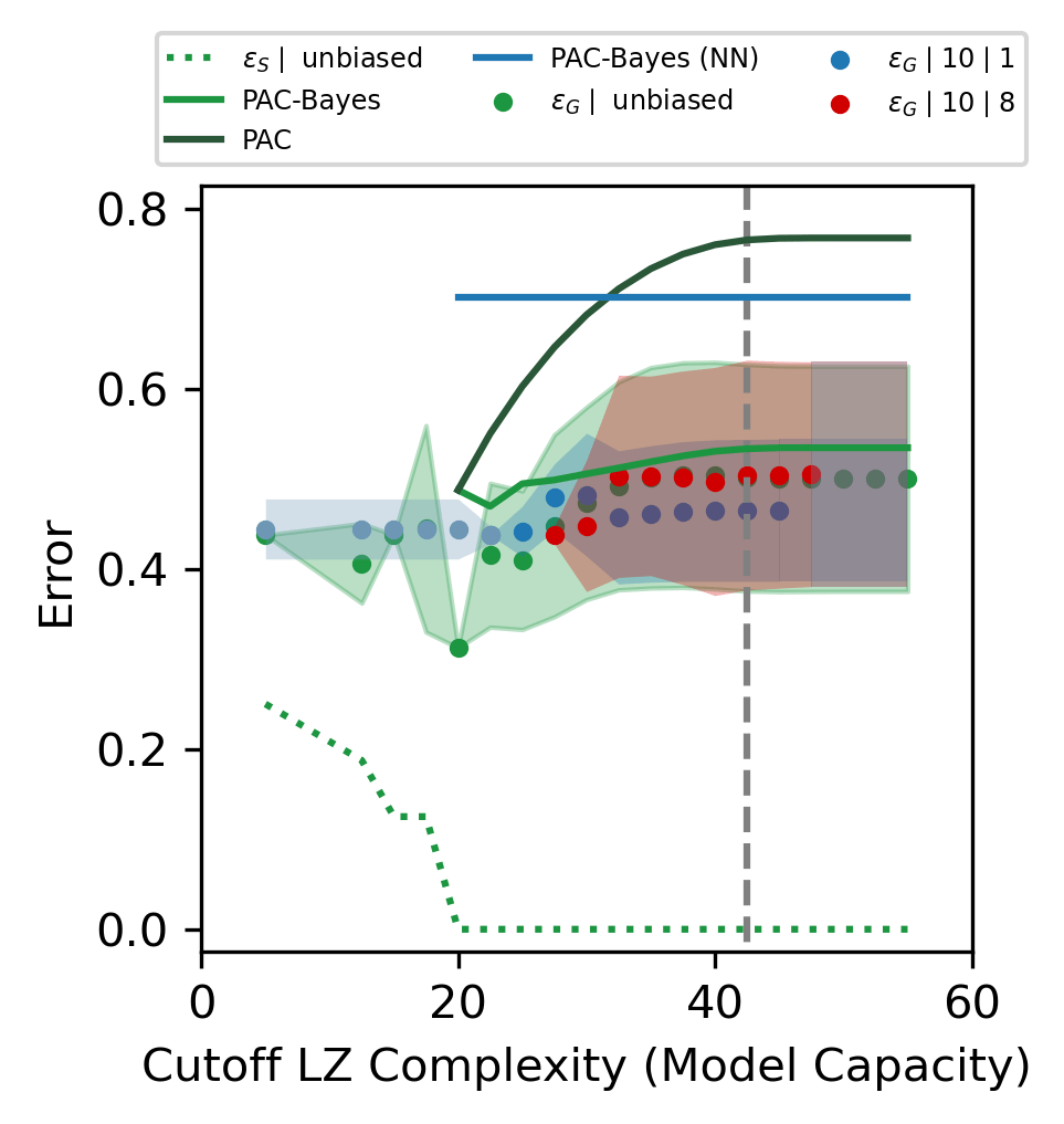
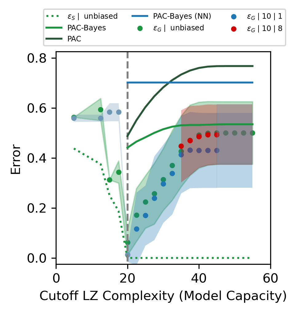
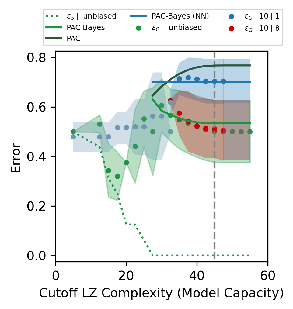
(a) ‘0011’ 8
(b) ‘01001111000111111110101111110100’
(c) ‘1001’ 8
(d) Parity function
A simple function (a) is learnable by the uniform learner with a hypothesis space restricted to the complexity of the target function, or the DNN with . A highly complex function (b) should not be learnable no matter the chosen training set and hypothesis restriction. (c) A simple function (with respect to LZ complexity) has very low prior probability (was not found during sampling the prior, so ) is a low-K low-P function. Therefore, the DNN with does not generalise that well either. (d) The parity function is clearly very hard for the DNN to learn. Interestingly it seems biased against it, as it generalises worse than a random learner. However, the parity function is learnable for the dataset with . (see Figure S17).
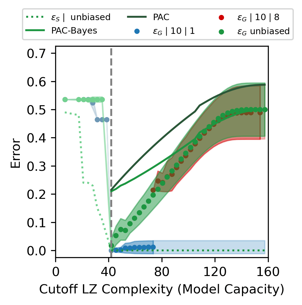
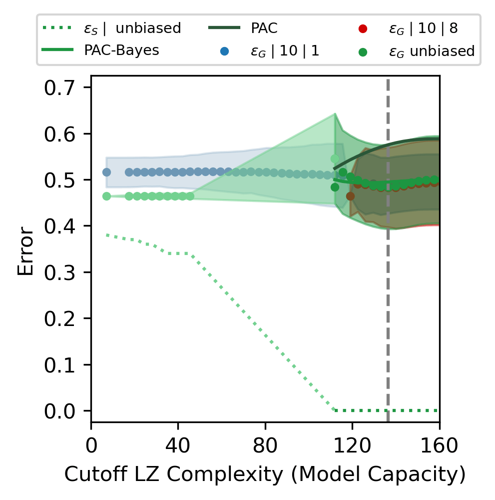
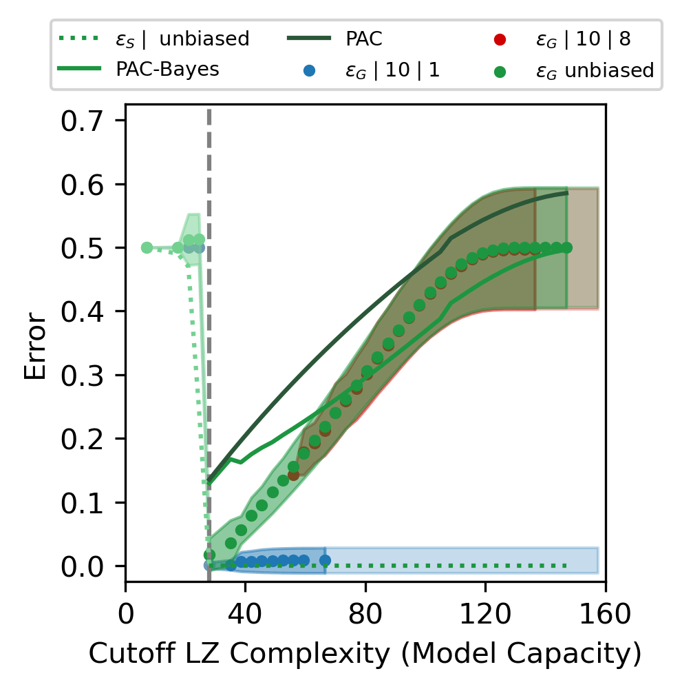
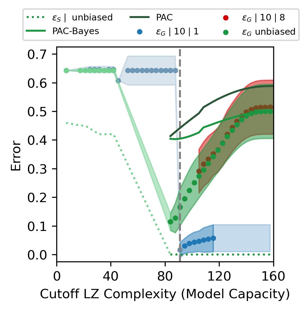
(a) simple function ‘10011010’ 16
(b) complex function ‘0011011110100111010010111001011100011100101110111011101011101111
0000110001100011111111100111011001111010010101011101111001110001’
(c)lowK lowP function at ‘1001’ 32
(d) Parity function
Unlike the case, good generalization is achieved for the lowK lowP function in (c) and parity function in (d). This may be due in part to the relatively large training set ().