Deterministic epidemic models overestimate the basic reproduction number of observed outbreaks

Abstract

The basic reproduction number, $R_{0}$, is a well-known quantifier of epidemic spread. However, a class of existing methods for estimating this quantity from epidemic incidence data can lead to an over-estimation of this quantity. In particular, when fitting deterministic models to estimate the rate of spread, we do not account for the stochastic nature of epidemics and that, given the same system, some outbreaks may lead to epidemics and some may not. Typically, an observed epidemic that we wish to control is a major outbreak. This amounts to implicit selection for major outbreaks which leads to the over-estimation problem. We show that by conditioning a ‘deterministic’ model on major outbreaks, we can more reliably estimate the basic reproduction number from an observed epidemic trajectory.

[inst1]organization=Department of Mathematical Sciences, University of Liverpool,addressline=Peach Street, city=Liverpool, postcode=L69 7ZX, state=England, country=United Kingdom

[inst2]organization=Department of Applied Mathematics, Liverpool John Moores University,addressline= Byrom Street, city=Liverpool, postcode=L3 5UX, state=England, country=United Kingdom

1 Introduction

A new, emerging infectious disease can potentially spread around the world within days or weeks, as observed during COVID-19 (Carvalho et al., 2021), and swine flu (Coker, 2009). During the early phase of an epidemic, estimation of key epidemiological parameters help us to estimate its future behaviour including the rate of spread, final size, and the requirements for effective control. In these early stages, epidemics typically exhibit exponential growth.

The basic reproduction number, $R_{0}$, is the number of secondary infections per primary infection in an otherwise susceptible population (Dietz, 1993; Heesterbeek and Dietz, 1996; Heffernan et al., 2005). The basic reproduction number has been shown to have important implications relating to the final epidemic size (Andreasen, 2011) and requirements for control (Lipsitch et al., 2003). It is also directly related to the early growth rate ($r$) of epidemics (Lipsitch et al., 2003; Ma, 2020) and both of these quantifiers are used for predicting the fate of outbreaks. That is, when $R_{0}$ is greater than $1$ (or $r$ is positive), then the introduction of an infected individual into a susceptible population may lead to a major epidemic.

Although epidemics are stochastic processes, it is sometimes convenient to use a deterministic approach such as the Kermack-Mckendrick SIR model (Kermack and McKendrick, 1927, 1932), SIS model (Lajmanovich and Yorke, 1976), SEIR Model (Anderson and May, 1992) or the exponential or logistic growth curves (Chowell et al., 2006). Unlike their stochastic counterparts (Whittle, 1955; Bailey, 1975), these models guarantee an epidemic when $R_{0}>1$ (Kermack and McKendrick, 1927). Such models have been used to estimate epidemic parameters by fitting them to real epidemic data, for example, influenza (Chowell et al., 2016), cholera (Pourabbas et al., 2001), and COVID-19 (Metelmann et al., 2021). We refer to (Ma et al., 2014) and (Ma, 2020) for more details on estimating early growth rates and the basic reproductive ratio from real data.

These classic models can be valuable but may lead to an overestimation of the basic reproduction number (Breban et al., 2007; Chowell, 2017; Green et al., 2006; Keeling and Grenfell, 2000). Generally, uncertainty in the estimation of parameters may arise due to noise in the data and/or the underlying assumptions for building models (Chowell, 2017). However, here we observe that there is also a fundamental bias in the deterministic models which occurs because they do not capture the stochastic effects in the early phases of an outbreak and, in particular, do not distinguish the possibility of stochastic fade-out when $R_{0}$ is greater than 1 (Whittle, 1955; Bailey, 1975). Similar issues with deterministic models and stochastic fade-out have been explored in (Overton et al., 2022) in the context of steady-state solutions to the SIS model.

By reducing them to a simple birth-death process, we show that SIR and SIS deterministic models implicitly average over both major and minor outbreaks during their early phases; that is both extinct and extant trajectories are included in the average behaviour. However, an observed epidemic is necessarily a major outbreak and therefore corresponds to an implicit conditioning on major outbreaks. This leads deterministic SIR and SIS models to overestimate the rate of transmission when they are fitted to epidemic data which we illustrate in the next section. This is more pronounced when the probability of minor outbreaks is large; i.e. when we have a small number of initial infections or when $R_{0}$ is close to $1$. In Section 3, we develop a conditioned simple birth-death process that better-describes a typical major outbreak and we show that this performs well in removing the bias from the estimation of $R_{0}$.

2 Estimation of $R_{0}$ using standard deterministic models

Consider an infectious disease that is spread via contact between susceptible and infected individuals. Let $\tau$ be the rate at which a single individual infects a susceptible individual during its infectious period and let $i(t)$ and $s(t)$ denote the infectious and susceptible populations respectively. We suppose that infection then occurs according to a Poisson process with rate $\tau si$. Similarly, we assume removal occurs according to a Poisson process with rate $\gamma i$ where $\gamma$ is the rate of removal of a single individual. This can be applied to infections that produce no long-term immunity (SIS or SIRS) or permanent immunity (SIR).

Moreover, in a sufficiently large population, the early phase of the epidemic behaves like a simple birth-death (BD) process. This can be seen from the infection rates $\tau si$; for a total population of size $N$ initiated with a single infected ($i_{0}=1$) in an otherwise susceptible population, the initial infection rates for $1,2,3,\dots$ infected individuals is $\tau(N-1),2\tau(N-2),3\tau(N-3),\dots$ respectively. These are approximately $i\tau N=\beta i$; that is, the susceptible population is approximately $N$ (Renshaw, 1993). So, the early phases of the infection dynamics are approximated by a simple birth-death process with individual birth rate $\beta$ and individual death rate $\gamma$. For comparison, both SIS and SIR processes and (their approximation) the simple BD process are summarised in Table 1, and the time series curves of the infected populations are illustrated in Fig. 1.

Event	SIS	SIR	BD
Infection	$(s,i)\xrightarrow{\tau si}(s-1,i+1)$	$(s,i)\xrightarrow{\tau si}(s-1,i+1)$	$i\xrightarrow{\beta i}i+1$
Recovery	$(s,i)\xrightarrow{\gamma i}(s+1,i-1)$	$(s,i)\xrightarrow{\gamma i}(s,i-1)$	$i\xrightarrow{\gamma i}i-1$

Table 1: State transitions in the SIS, SIR and the simple Birth-Death (BD) processes.

(a) Averages of SIR process

(b) Averages of SIS process

(c) Averages of BD process

Figure 1: The average of 10,000 simulations (solid line) and those conditioned against extinction (dashed line) for (a) the SIR process, (b) the SIS process and (c) the simple Birth-Death (BD) process. In each case, $\beta=1.5$, $\gamma=1$, $N=1000$ and the initial number infected is $i_{0}=1$.

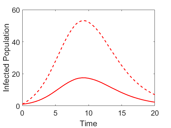
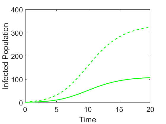
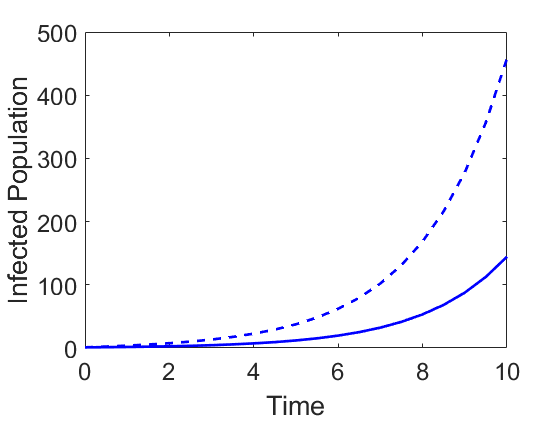
The expected number of infected individuals (denoted by $\langle i\rangle$) in the simple BD process at a given time $t$ can be derived from the master equation for the process. Let the probability that there are $i$ infected individuals at time $t$ be denoted by $p_{i}(t)$, where $i\in\{0,1\dots\}$. Thus, the master equation for the simple birth-death process is given by:

$$\frac{d}{dt}p_{i}(t)=\beta(i-1)p_{i-1}(t)-(\beta+\gamma)ip_{i}(t)+\gamma(i+1)p_{i+1}(t).$$ (1)

From this, the rate of change of the expected infectious population is (Feller, 1939; Kendall, 1948):

$$\frac{d}{dt}\langle i\rangle=\sum_{i}i\frac{d}{dt}p_{i}(t)=(\beta-\gamma)\langle i\rangle.$$ (2)

This has the same form as the deterministic simple BD model given in Table 2, so the deterministic BD model describes the average of all stochastic realisations of the stochastic BD process. Similar connections can be established between the stochastic and deterministic SIS and SIR models under some closure approximations (Sharkey et al., 2015; Kiss et al., 2017; Overton et al., 2022).

SIS	SIR	BD
$\!\begin{aligned} \frac{dS}{dt}&=-\tau SI+\gamma I\\ \frac{dS}{dt}&=\tau SI-\gamma I\end{aligned}$	$\!\begin{aligned} \frac{dS}{dt}&=-\tau SI\\ \frac{dS}{dt}&=\tau SI-\gamma I\\ \frac{dR}{dt}&=\gamma I\par\end{aligned}$	$\!\begin{aligned} \frac{dI}{dt}=\beta I-\gamma I\end{aligned}$

Table 2: Equations for deterministic SIS, SIR and BD models where $S$, $I$, $R$ are the sizes of the classes of susceptible, infected and removed respectively. The parameters $\tau$ and $\gamma$ are the transmission and recovery (or removal) rates. Here, for convenience we have used the same parameter notation as for the stochastic models.

Moreover, the deterministic BD model (and equivalently Equation 2) describes the expected early deterministic dynamics of both SIS and SIR processes when $N$ is large. This is because (see Table 2) the deterministic SIS and SIR (and SIRS) models have the following equation for the infectious population (Kermack and McKendrick, 1927):

$$\frac{dI}{dt}=\tau SI-\gamma I,$$ (3)

where we use capital letters $I$ and $S$ for denoting the number of infected and susceptible individuals in deterministic models. This reduces to Equation 2 under the same approximation as we applied to the stochastic models (i.e. $S\approx N$ with $\beta=\tau N$) and so the expected behaviour of the stochastic SIR and SIS models is approximated by the deterministic SIR and SIS models, and by the BD model (Equation 2) in the early stages.

The equivalence of the deterministic models to the expected value of the stochastic models and their derivation from the master equation tells us that the deterministic models represent an averaging over all epidemic outcomes (Overton et al., 2022). Crucially this averaging is over both major and minor outbreaks. However, necessarily, a real epidemic of interest is a major outbreak and this therefore represents conditioning on major outbreaks.

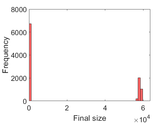
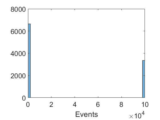
Fig. 2(a) shows the distribution of final sizes (Andreasen, 2011) of an SIR process when initiated with a single infected individual. The bimodal nature of this distribution tells us that that a group of realisations generate major outbreaks while others go extinct in the early phase after some or no secondary infections. Fig. 2(b) shows similar bimodal behaviour for SIS dynamics where here the process is run until either extinction or until $2N$ events have occurred. Although the split between major and minor outbreaks is usually obvious, it is not well-defined in finite populations. Throughout this paper we choose to formally characterise the split between major and minor outbreaks by using Otsu’s method (Otsu, 1979) which gives a threshold value for clustering bimodal histograms and provides us with a working definition.

(a) Final sizes in SIR process

(b) Infection events in SIS process

Figure 2: (a) The final size distribution obtained from $10,000$ stochastic simulations of SIR dynamics and (b) the distribution in the number of (infection and recovery) events for 10,000 SIS simulations capped at $2N$ events. In both sets of simulations, $N=10,000$, $\beta=1.5$, $\gamma=1$, and the initial number infected is $i_{0}=1$.

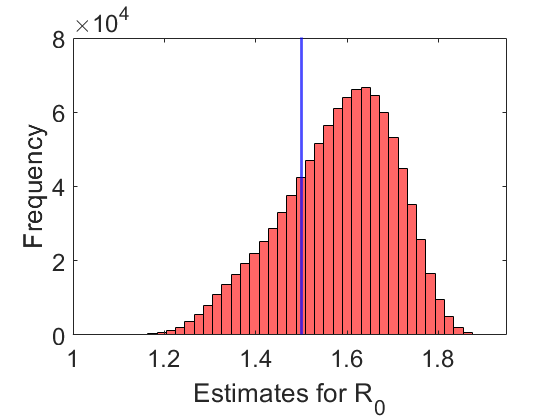
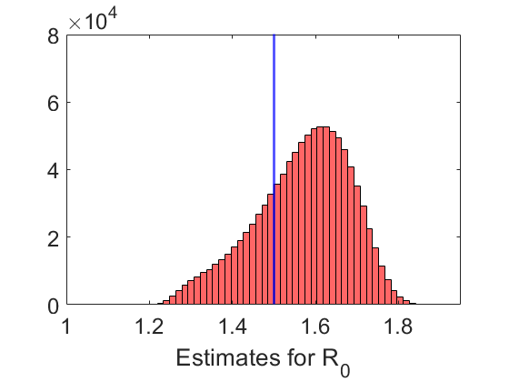
To illustrate the issue of over-estimation, we performed least-square fits of both deterministic SIR and SIS models to simulated major outbreaks of both types to estimate the transmission rate $\beta$, assuming that we know $\gamma$ (here $\gamma=1$). $R_{0}$ is then calculated from $R_{0}=\beta/\gamma$ (Keeling and Grenfell, 2000; van den Driessche, 2017). The resulting distributions in $R_{0}$ values are shown for both SIR (Fig. 3(a)) and SIS (Fig. 3(b)). Both distributions clearly show an upwards bias in the estimates with respect to the “true” value of $R_{0}=1.5$ used to generate the stochastic simulations. Thus, fitting mean-field SIS and SIR models (or the simple BD model) to major real outbreak data will have a tendency to overestimate the transmission rate and overestimate $R_{0}$.

(a) Fitting SIR model to data

(b) Fitting SIS model to data

Figure 3: The distributions of $R_{0}$ estimated by performing least squares fits of (a) the SIR model and (b) the SIS model to $1$ million major outbreaks of each type generated by taking $\beta=1.5$, $\gamma=1$, $N=100,000$ and the initial number infected $i_{0}=1$. The blue lines in both plots represent the actual value of $R_{0}$ used to generate the simulated outbreaks. The fitting window for both histograms is $t\in[0,10]$.

To resolve this and obtain a deterministic model that we can fit to the early phases of epidemics to determine $R_{0}$, we need to account for this conditioning on major outbreaks. Since the early stages of SIS and SIR dynamics are well-approximated by the simple BD process, we look to develop a simple BD process which is conditioned on major outbreaks.

3 Estimation of $R_{0}$ using a conditioned BD model

We wish to calculate the conditional probability $P(\textrm{$i$ infected at time $t|$ major outbreak})$ for the simple BD process. To make analytic progress, we approximate this probability by:

$$P(\textrm{$i$ infected at time $t|$ major outbreak})\approx q_{i}(t)$$

where

$$q_{i}(t)=P(\textrm{$i$ infected at time $t|i\neq 0$ at time $t$})$$

for $i\in\{1\dots\}$. This leads to

$$q_{i}(t)=\frac{p_{i}(t)}{1-p_{0}(t)}$$

where, with reference to Equation 1, the probability that the disease has died out at time $t$, is denoted by $p_{0}(t)$.

Differentiating gives:

$$\begin{array}[]{ccc}\frac{d}{dt}q_{i}(t)=\frac{\frac{d}{dt}p_{i}(t)}{1-p_{0}(t)}+\frac{p_{i}(t)}{\left[1-p_{0}(t)\right]^{2}}\frac{d}{dt}p_{0}(t),&\text{for}&i=1,2,\dots.\end{array}$$

where using the expression for $dp_{i}(t)/dt$ given in Equation 1 when $i\neq 0$, and using $dp_{0}(t)/dt=\gamma p_{1}(t)$ and $q_{i}(t)=p_{i}(t)/(1-p_{0}(t))$, we reach the following model:

$$\frac{d}{dt}q_{i}(t)=\beta(i-1)q_{i-1}(t)-(\beta+\gamma)iq_{i}(t)+\gamma(i+1)q_{i+1}+\gamma q_{1}q_{i}(t).$$

We now derive an equation for the rate of change of the expected number of infected individuals at time $t$:

$$\langle i\rangle_{c}(t)=\sum_{i=1}iq_{i}(t),$$

where the subscript $c$ indicates that this is the expected value in the conditioned process. Differentiating with respect to time and substituting for $dq_{i}(t)/dt$ from Equation 3:

$$\frac{d}{dt}\langle i\rangle_{c}=\beta\sum_{i=1}i(i-1)q_{i-1}(t)-(\beta+\gamma)\sum_{i=1}i^{2}q_{i}(t)+\gamma\sum_{i=1}i(i+1)q_{i+1}+\gamma q_{1}\langle i\rangle_{c}.$$

The summation in the first term on the right-hand-side can be written as:

$$\sum_{i=1}i(i-1)q_{i-1}(t)=\sum_{k=0}(k+1)(k)q_{k}(t)=\sum_{i=1}i^{2}q_{i}(t)+\sum_{i=1}iq_{i}(t),$$

and the summation in the third term on the right-hand-side can be written as:

$$\sum_{i=1}i(i+1)q_{i+1}(t)=\sum_{k=2}(k-1)(k)q_{k}(t)=\sum_{i=2}i^{2}q_{i}(t)-\sum_{i=2}iq_{i}(t).$$

This leads to:

$$\frac{d}{dt}\langle i\rangle_{c}=(\beta-\gamma)\langle i\rangle_{c}+\gamma\langle i\rangle_{c}q_{1}.$$ (4)

This system is not closed because we have one extra variable $q_{1}$, which is the probability of single infection in the conditioned process. However, using the exact solution of Equation 1 (Kot, 2001, Chapter 3), (Renshaw, 1993) we can write an exact expression for $q_{1}$:

$$q_{1}(t)=\frac{p_{1}(t)}{1-p_{0}(t)}$$

where

$$p_{0}(t)=\left\{\begin{array}[]{cc}\left[\frac{\beta t}{1+\beta t}\right]^{i_{0}},&\beta=\gamma\\ \left[\frac{\gamma(e^{rt}-1)}{\beta e^{et}-\gamma}\right]^{i_{0}},&\beta\neq\gamma\end{array}\right.$$

and

$$p_{1}(t)=\left\{\begin{array}[]{cc}i_{0}\left[\frac{\beta t}{1+\beta t}\right]^{i_{0}-1}\frac{1}{(1+\beta t)^{2}},&\beta=\gamma\\ i_{0}\alpha^{i_{0}-1}\left[(1-\alpha)(1-\phi)\right],&\beta\neq\gamma.\end{array}\right.$$

Here $i_{0}$ is the initial number of infected and

$$\begin{array}[]{ccc}\alpha=\frac{\gamma(e^{rt}-1)}{\beta e^{rt}-\gamma},&&\phi=\frac{\beta(e^{rt}-1)}{\beta e^{rt}-\gamma},\\ \end{array}$$

where, $r=\beta-\gamma$.

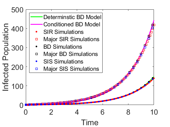
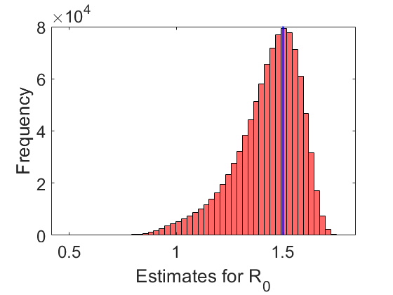
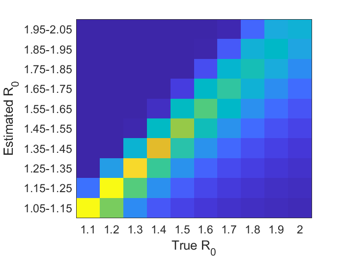
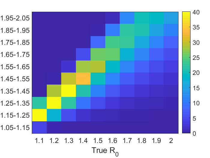
As discussed in Section 2, the early phase of the SIS and SIR epidemic models are well-approximated by the simple BD process. Similarly the conditional (SIS and SIR) epidemic processes are also well-approximated the conditional stochastic BD process. Conditioned and non-conditioned processes lead to different average trajectories (Fig. 4(a)) and it can be seen that the new conditioned BD model (Equation 4) accurately describes the early part of the SIR, SIS and BD expected behaviour when conditioned on major outbreaks. This new model resolves the issue of upward bias which we saw in Fig. 3(a). When it is fitted to major outbreaks of SIR epidemics, we can see in Fig. 4(b) that the distribution of estimated $R_{0}$ values is centred around the true value. Fig. 5(a) explores the parameter space for small $R_{0}$ more fully and shows a significantly improved estimate of $R_{0}$ when compared with the standard SIR model (Fig. 5(b)). The fitting window for Fig. 4(b) and Fig. 5 is the time interval $t\in[0\,\,T]$ where we determined $T$ to be the time point at which the simple BD approximation gives a 1% error in the estimation of the infectious time series in the SIR process.

(a) Models vs simulations

(b) Fitting CBD model to data

Figure 4: (a) The deterministic conditioned (against extinction) and unconditioned BD models together with averages of 100,000 conditioned and unconditioned BD, SIS and SIR simulations. (b) Estimates of $R_{0}$ by least-square fits of the conditioned BD Model (Equation 4) to 1 million major type outbreaks. The fitting window used is $t\in[0,9.52]$ which is determined so that the deterministic simple BD model is within $1\%$ of the SIR infectious time series. For both subplots, $i_{0}=1$, $\beta=1.5$, $\gamma=1$ and $N=100,000$.

(a) CBD Model

(b) SIR Model

Figure 5: The distribution of estimated $R_{0}$ values by fitting (a) the conditioned BD model and (b) the SIR model. Both these models are fitted to 1 million simulated major SIR outbreaks per $R_{0}$ value. The horizontal axis corresponds to the “true” values of $R_{0}$. The vertical axis corresponds to the histograms of estimated $R_{0}$ (similar to Figure 4(b)). Here, the intensity of the color indicates the percentage of estimates in each interval.

4 Discussion

One method for obtaining the basic reproduction number ($R_{0}$) from real data is to fit deterministic models to epidemic data (Breban et al., 2007; Chowell, 2017; van den Driessche, 2017; Green et al., 2006; Keeling and Grenfell, 2000; Ma, 2020). Here we showed that some of these deterministic models are fundamentally biased in their estimation of $R_{0}$ (Breban et al., 2007; Chowell, 2017). We showed this explicitly in the context of SIS and SIR epidemic dynamics (Fig. 3(a) and 3(b)) where we can make some analytic progress. Trivially this also applies directly to SIRS models as well (Mena-Lorcat and Hethcote, 1992).

The early phases of both the stochastic SIS and SIR epidemic processes and the deterministic SIS and SIR models reduce to a simple birth-death process (see, for example, (Renshaw, 1993)), and so the early behaviour of the deterministic models describes the expected behaviour of all possible epidemic realisations. The over-estimation of $R_{0}$ occurs because a real epidemic of interest is necessarily a major outbreak, representing an implicit conditioning against early extinction.

We resolved this by developing a simple birth-death model with conditioning against extinction (Equation 4). To do this, we made use of the analytic solution of the simple birth-death master equation. We showed that fitting this model to the early stages of epidemic outbreaks resolves the issue of overestimation of $R_{0}$ (Fig. 4(b) and 5(a)).

It is expected that similar issues would apply to other epidemic models such as SEIR type models (Anderson and May, 1992) and models that do not rely on Poisson processes ((Kenah, 2011; KhudaBukhsh et al., 2020)). It would be of interest to determine the extent of this error in these scenarios. For this, we currently lack the ingredients that we made use of which are the approximation of SIS and SIR dynamics by the simple birth-death (BD) process, the analytic solution of the BD process and the equivalence of the deterministic BD and the average stochastic BD processes. Nevertheless, this implicit conditioning on major outbreaks seems likely to cause problems with these models as well. The approximation to the conditioned SIS model proposed in (Overton et al., 2022) can also be extended to cover transient dynamics and to model more complex epidemiological structures.

References

- Anderson and May (1992) Anderson, R., May, R., 1992. Infectious diseases of humans: dynamics and control.
- Andreasen (2011) Andreasen, V., 2011. The final size of an epidemic and its relation to the basic reproduction number. Bulletin of Mathematical Biology 73, 2305–2321. doi:10.1007/s11538-010-9623-3.
- Bailey (1975) Bailey, N., 1975. The elements of stochastic processes with applications to the natural sciences.
- Breban et al. (2007) Breban, R., Vardavas, R., Blower, S., 2007. Theory versus data: How to calculate r0? PLoS ONE 2. doi:10.1371/JOURNAL.PONE.0000282.
- Carvalho et al. (2021) Carvalho, T., Krammer, F., Iwasaki, A., 2021. The first 12 months of covid-19: a timeline of immunological insights. Nature Reviews Immunology 21, 245–256. doi:10.1038/s41577-021-00522-1.
- Chowell (2017) Chowell, G., 2017. Fitting dynamic models to epidemic outbreaks with quantified uncertainty: A primer for parameter uncertainty, identifiability, and forecasts. Infectious Disease Modelling 2, 379–398. doi:10.1016/J.IDM.2017.08.001.
- Chowell et al. (2006) Chowell, G., Ammon, C., Hengartner, N., Hyman, J., 2006. Transmission dynamics of the great influenza pandemic of 1918 in geneva, switzerland: Assessing the effects of hypothetical interventions. Journal of Theoretical Biology 241, 193–204. doi:10.1016/j.jtbi.2005.11.026.
- Chowell et al. (2016) Chowell, G., Sattenspiel, L., Bansal, S., Viboud, C., 2016. Mathematical models to characterize early epidemic growth: A review. Physics of Life Reviews 18, 66–97. doi:10.1016/j.plrev.2016.07.005.
- Coker (2009) Coker, R., 2009. Swine flu. BMJ 338, b1791–b1791. doi:10.1136/bmj.b1791.
- Dietz (1993) Dietz, K., 1993. The estimation of the basic reproduction number for infectious diseases. Statistical Methods in Medical Research 2, 23–41. doi:10.1177/096228029300200103.
- van den Driessche (2017) van den Driessche, P., 2017. Reproduction numbers of infectious disease models. Infectious Disease Modelling 2, 288–303. doi:10.1016/J.IDM.2017.06.002.
- Feller (1939) Feller, W., 1939. Die grundlagen der volterraschen theorie des kampfes ums dasein in wahrscheinlichkeitstheoretischer behandlung. Acta Biotheoretica 5, 11–40. doi:10.1007/BF01602932/METRICS.
- Green et al. (2006) Green, D.M., Kiss, I.Z., Kao, R.R., 2006. Parameterization of individual-based models: comparisons with deterministic mean-field models. Journal of theoretical biology 239, 289–297. doi:10.1016/J.JTBI.2005.07.018.
- Heesterbeek and Dietz (1996) Heesterbeek, J.A.P., Dietz, K., 1996. The concept of r0 in epidemic theory. Statistica Neerlandica 50, 89–110. doi:10.1111/j.1467-9574.1996.tb01482.x.
- Heffernan et al. (2005) Heffernan, J., Smith, R., Wahl, L., 2005. Perspectives on the basic reproductive ratio. Journal of The Royal Society Interface 2, 281–293. doi:10.1098/rsif.2005.0042.
- Keeling and Grenfell (2000) Keeling, M.J., Grenfell, B.T., 2000. Individual-based perspectives on r0. Journal of Theoretical Biology 203, 51–61. doi:10.1006/JTBI.1999.1064.
- Kenah (2011) Kenah, E., 2011. Contact intervals, survival analysis of epidemic data, and estimation of r0. Biostatistics 12, 548–566. doi:10.1093/BIOSTATISTICS/KXQ068.
- Kendall (1948) Kendall, D.G., 1948. On the generalized ”birth-and-death” process. https://doi.org/10.1214/aoms/1177730285 19, 1–15. doi:10.1214/AOMS/1177730285.
- Kermack and McKendrick (1927) Kermack, W.O., McKendrick, W.O.A.G., 1927. A contribution to the mathematical theory of epidemics. Proceedings of the Royal Society of London. Series A, Containing Papers of a Mathematical and Physical Character 115, 700–721. doi:10.1098/rspa.1927.0118.
- Kermack and McKendrick (1932) Kermack, W.O., McKendrick, W.O.A.G., 1932. Contributions to the mathematical theory of epidemics. ii. —the problem of endemicity. Proceedings of the Royal Society of London. Series A, Containing Papers of a Mathematical and Physical Character 138, 55–83. doi:10.1098/rspa.1932.0171.
- KhudaBukhsh et al. (2020) KhudaBukhsh, W.R., Choi, B., Kenah, E., Rempała, G.A., 2020. Survival dynamical systems: individual-level survival analysis from population-level epidemic models. Interface Focus 10. doi:10.1098/RSFS.2019.0048.
- Kiss et al. (2017) Kiss, I.Z., Miller, J.C., Simon, P.L., 2017. Mathematics of Epidemics on Networks: From Exact to Approximate Models. volume 46. Springer International Publishing. doi:10.1007/978-3-319-50806-1.
- Kot (2001) Kot, M., 2001. Elements of Mathematical Ecology. Cambridge University Press.
- Lajmanovich and Yorke (1976) Lajmanovich, A., Yorke, J.A., 1976. A deterministic model for gonorrhea in a nonhomogeneous population. Mathematical Biosciences 28, 221–236. doi:10.1016/0025-5564(76)90125-5.
- Lipsitch et al. (2003) Lipsitch, M., Cohen, T., Cooper, B., Robins, J.M., Ma, S., James, L., Gopalakrishna, G., Chew, S.K., Tan, C.C., Samore, M.H., Fisman, D., Murray, M., 2003. Transmission dynamics and control of severe acute respiratory syndrome. Science 300, 1966–1970. doi:10.1126/science.1086616.
- Ma (2020) Ma, J., 2020. Estimating epidemic exponential growth rate and basic reproduction number. Infectious Disease Modelling 5, 129–141. doi:10.1016/j.idm.2019.12.009.
- Ma et al. (2014) Ma, J., Dushoff, J., Bolker, B.M., Earn, D.J., 2014. Estimating initial epidemic growth rates. Bulletin of Mathematical Biology 76, 245–260. doi:10.1007/S11538-013-9918-2/FIGURES/6.
- Mena-Lorcat and Hethcote (1992) Mena-Lorcat, J., Hethcote, H.W., 1992. Dynamic models of infectious diseases as regulators of population sizes. Journal of Mathematical Biology 30, 693–716. doi:10.1007/BF00173264.
- Metelmann et al. (2021) Metelmann, S., Pattni, K., Brierley, L., Cavalerie, L., Caminade, C., Blagrove, M.S., Turner, J., Sharkey, K.J., Baylis, M., 2021. Impact of climatic, demographic and disease control factors on the transmission dynamics of covid-19 in large cities worldwide. One Health 12, 100221. doi:10.1016/j.onehlt.2021.100221.
- Otsu (1979) Otsu, N., 1979. Threshold selection method from gray-level histograms. IEEE Trans Syst Man Cybern SMC-9, 62–66. doi:10.1109/TSMC.1979.4310076.
- Overton et al. (2022) Overton, C.E., Wilkinson, R.R., Loyinmi, A., Miller, J.C., Sharkey, K.J., 2022. Approximating quasi-stationary behaviour in network-based sis dynamics. Bulletin of Mathematical Biology 84, 1–32. doi:10.1007/S11538-021-00964-7/FIGURES/4.
- Pourabbas et al. (2001) Pourabbas, E., d’Onofrio, A., Rafanelli, M., 2001. A method to estimate the incidence of communicable diseases under seasonal fluctuations with application to cholera. Applied Mathematics and Computation 118, 161–174. doi:10.1016/S0096-3003(99)00212-X.
- Renshaw (1993) Renshaw, E., 1993. Modelling Biological Populations in Space and Time. Cambridge University Press.
- Sharkey et al. (2015) Sharkey, K.J., Kiss, I.Z., Wilkinson, R.R., Simon, P.L., 2015. Exact equations for sir epidemics on tree graphs. Bull Math Biol 77, 614–645. doi:10.1007/s11538-013-9923-5.
- Whittle (1955) Whittle, P., 1955. The outcome of a stochastic epidemic-a note on bailey’s paper. Biometrika 42, 116–122. doi:10.1093/BIOMET/42.1-2.116.