DiffFit: Unlocking Transferability of Large Diffusion Models
via Simple Parameter-Efficient Fine-Tuning
Abstract
Diffusion models have proven to be highly effective in generating high-quality images. However, adapting large pre-trained diffusion models to new domains remains an open challenge, which is critical for real-world applications. This paper proposes DiffFit, a parameter-efficient strategy to fine-tune large pre-trained diffusion models that enable fast adaptation to new domains. DiffFit is embarrassingly simple that only fine-tunes the bias term and newly-added scaling factors in specific layers, yet resulting in significant training speed-up and reduced model storage costs. Compared with full fine-tuning, DiffFit achieves 2 training speed-up and only needs to store approximately 0.12% of the total model parameters. Intuitive theoretical analysis has been provided to justify the efficacy of scaling factors on fast adaptation. On 8 downstream datasets, DiffFit achieves superior or competitive performances compared to the full fine-tuning while being more efficient. Remarkably, we show that DiffFit can adapt a pre-trained low-resolution generative model to a high-resolution one by adding minimal cost. Among diffusion-based methods, DiffFit sets a new state-of-the-art FID of 3.02 on ImageNet 512512 benchmark by fine-tuning only 25 epochs from a public pre-trained ImageNet 256256 checkpoint while being 30 more training efficient than the closest competitor.
1 Introduction
Denoising diffusion probabilistic models (DDPMs) [27, 68, 66] have recently emerged as a formidable technique for generative modeling and have demonstrated impressive results in image synthesis [58, 15, 60], video generation [28, 26, 90] and 3D editing [55]. However, the current state-of-the-art DDPMs suffer from significant computational expenses due to their large parameter sizes and numerous inference steps per image. For example, the recent DALL E 2 [60] comprises 4 separate diffusion models and requires 5.5B parameters. In practice, not all users are able to afford the necessary computational and storage resources. As such, there is a pressing need to explore methods for adapting publicly available, large, pre-trained diffusion models to suit specific tasks effectively. In light of this, a central challenge arises: Can we devise an inexpensive method to fine-tune large pre-trained diffusion models efficiently?
Take the recent popular Diffusion Transformer (DiT) as an example, the DiT-XL/2 model, which is the largest model in the DiT family and yields state-of-the-art generative performance on the ImageNet class-conditional generation benchmark. In detail, DiT-XL/2 comprises 640M parameters and involves computationally demanding training procedures. Our estimation indicates that the training process for DiT-XL/2 on 256256 images necessitates 950 V100 GPU days (7M iterations), whereas the training on 512512 images requires 1733 V100 GPU days (3M iterations). The high computational cost makes training DiT from scratch unaffordable for most users. Furthermore, extensive fine-tuning of the DiT on diverse downstream datasets requires storing multiple copies of the whole model, which results in linear storage expenditures.
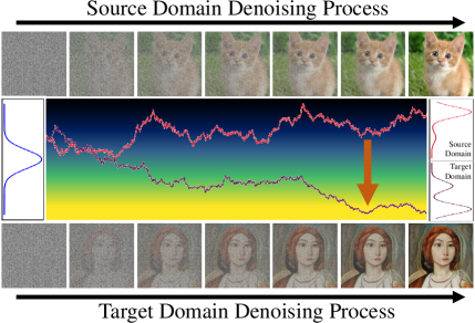
In this paper, we propose DiffFit, a simple and parameter-efficient fine-tuning strategy for large diffusion models, building on the DiT as the base model. The motivation can be found in Figure 2. Recent work in natural language processing (BitFit [83]) has demonstrated that fine-tuning only the bias term in a pre-trained model performs sufficiently well on downstream tasks. We, therefore, seek to extend these efficient fine-tuning techniques to image generative tasks. We start with directly applying BitFit [83] and empirically observe that simply using the BitFit technique is a good baseline for adaptation. We then introduce learnable scaling factors to specific layers of the model, initialized to 1.0, and made dataset-specific to accommodate enhancement of feature scaling and results in better adaptation to new domains. Interestingly, the empirical findings show that incorporating at specific locations of the model is important to reaching a better FID score. In other words, the FID score does not improve linearly with the number of included in the model. In addition, we conducted a theoretical analysis of the mechanism underlying the proposed DiffFit for fine-tuning large diffusion models. We provided intuitive theoretical analysis to help understand the effect of the newly-added scaling factors in the shift of distributions.
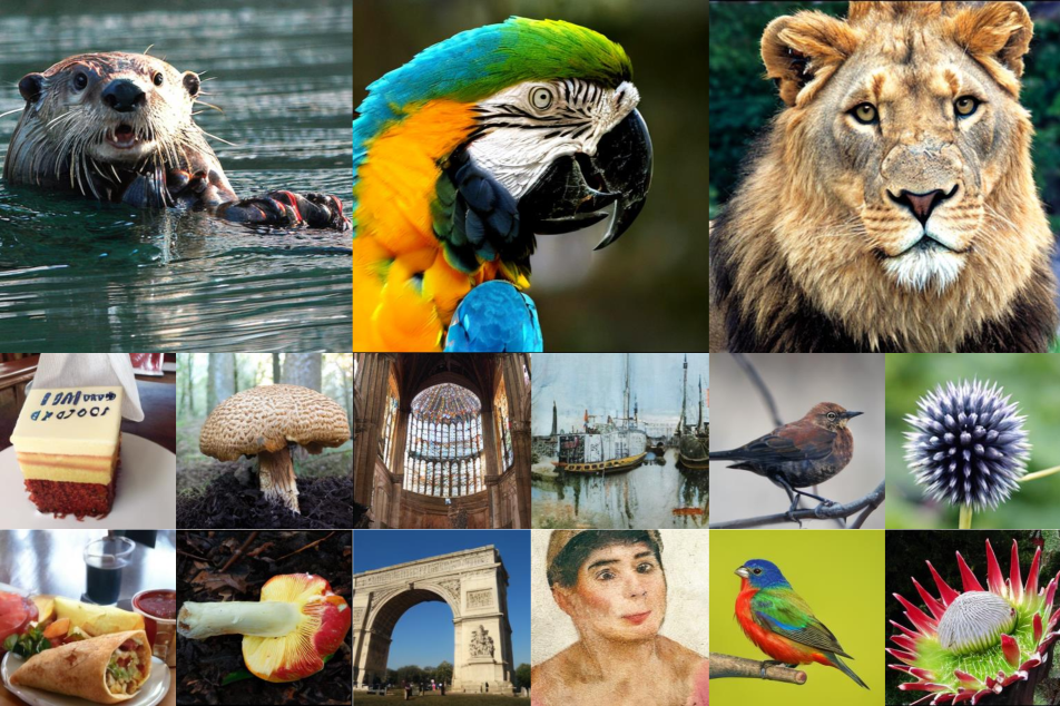
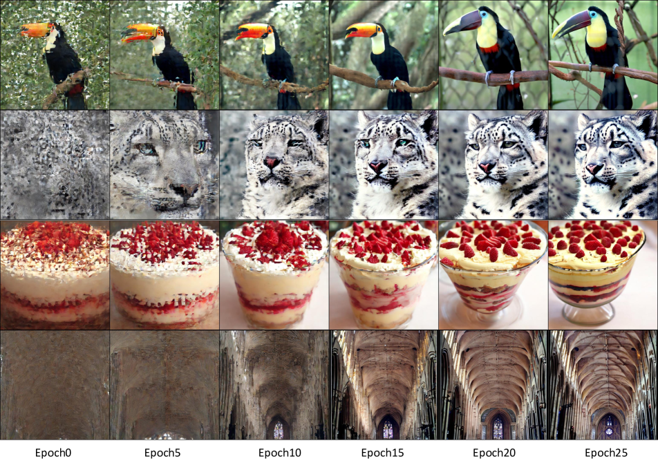
We employed several parameter-efficient fine-tuning techniques, including BitFit [83], AdaptFormer [9], LoRA [30], and VPT [31], and evaluated their performance on 8 downstream datasets. Our results demonstrate that DiffFit outperforms these methods regarding Frechet Inception Distance (FID) [52] trade-off and the number of trainable parameters. Furthermore, we surprisingly discovered that by treating high-resolution images as a special domain from low-resolution ones, our DiffFit approach could be seamlessly applied to fine-tune a low-resolution diffusion model, enabling it to adapt to high-resolution image generation at a minimal cost. For example, starting from a pre-trained ImageNet 256256 checkpoint, by fine-tuning DIT for only 25 epochs (0.1M iterations), DiffFit surpassed the previous state-of-the-art diffusion models on the ImageNet 512512 setting. Even though DiffFit has only about 0.9 million trainable parameters, it outperforms the original DiT-XL/2-512 model (which has 640M trainable parameters and 3M iterations) in terms of FID (3.02 vs. 3.04), while reducing 30 training time. In conclusion, DiffFit aims to establish a simple and strong baseline for parameter-efficient fine-tuning in image generation and shed light on the efficient fine-tuning of larger diffusion models.
Our contributions can be summarized as follows:
-
1.
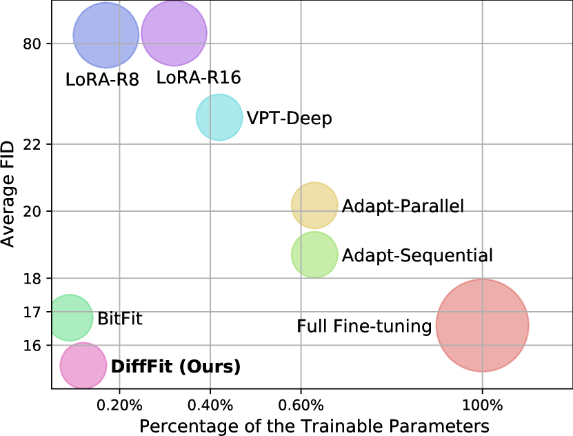
We propose a simple parameter-efficient fine-tuning approach for diffusion image generation named DiffFit. It achieves superior results compared to full fine-tuning while leveraging only 0.12% trainable parameters. Quantitative evaluations across 8 downstream datasets demonstrate that DiffFit outperforms existing well-designed fine-tuning strategies (as shown in Figure 3 and Table 1).
-
2.
We conduct an intuitive theoretical analysis and design detailed ablation studies to provide a deeper understanding of why this simple parameter-efficient fine-tuning strategy can fast adapt to new distributions.
-
3.
We show that by treating high-resolution image generation as a downstream task of the low-resolution pre-trained generative model, DiffFit can be seamlessly extended to achieve superior generation results with FID 3.02 on ImageNet and reducing training time by 30 times, thereby demonstrating its scalability.
2 Related Works
2.1 Transformers in Vision
Transformer architecture was first introduced in language model [73] and became dominant because of its scalability, powerful performance and emerging ability [56, 57, 4]. Then, Vision Transformer (ViT) [16] and its variants achieved colossal success and gradually replaced ConvNets in various visual recognition tasks, e.g. image classification [71, 89, 82, 23], object detection [45, 77, 78, 6], semantic segmentation [87, 80, 69] and so on [70, 41, 86, 47, 24, 40]. Transformers are also widely adopted in GAN-based generative models [18, 32] and the conditional part of text-to-image diffusion models [60, 62, 58, 1]. Recently, DiT [53] proposed a plain Transformer architecture for the denoising portion of diffusion networks and verified its scaling properties. Our paper adopts DiT as a strong baseline and studies parameter-efficient fine-tuning.
2.2 Diffusion Models
Diffusion models [27] (aka. score-based models [67]) have shown great success in generative tasks, including density estimation [33], image synthesis [15], text-to-image generation [60, 1, 63] and so on. Different from previous generative models like GAN [11], VAE [34] and Flow [59], diffusion models [27] transform a data distribution to a Gaussian distribution by progressively adding noise, and then, reversing the process via denoising to retrieve the original distribution. The progressive step-by-step transformation between the two distributions makes the training process of diffusion models more stable compared to other models. However, the multiple time-step generations makes the diffusion process time-consuming and expensive.
2.3 Parameter-efficient Fine-tuning
Witnessing the success of Transformers in language and vision, many large models based on Transformer architecture have been developed and pre-trained on massive upstream data. On the one hand, the industry continues to increase the model parameters to billion, even trillion scales [4, 19, 14] to probe up the upper bound of large models. On the other hand, fine-tuning and storage of large models are expensive. There are three typical ways for parameter-efficient fine-tuning as follows:
1. Adaptor [29, 30, 9]. Adaptor is a small module inserted between Transformer layers, consisting of a down-projection, a nonlinear activation function, and an up-projection. Specifically, LoRA [30] adds two low-rank matrices to the query and value results between the self-attention sub-layer. AdaptFormer [9], however, places the trainable low-rank matrices after the feed-forward sub-layer.
2. Prompt Tuning [39, 37, 49, 31, 91]. Usually, prefix tuning [39] appends some tunable tokens before the input tokens in the self-attention module at each layer. In contrast, prompt-tuning [37] only appends the tunable tokens in the first layer for simplification. VPT [31] focuses on the computer vision field and proposes deep and shallow prompt tuning variants.
3. Partial Parameter Tuning [83, 81, 42]. Compared with the above parameter-efficient methods, partial parameter tuning does not insert any other components and only fine-tunes the partial parameters of the original model. For example, BitFit [83] tunes the bias of each linear projection and Child-Tuning [81] evaluates the importance of parameters and tunes only the important ones.
3 Methodology
3.1 Preliminaries
Diffusion Models.
Denoising diffusion probabilistic models (DDPMs) [27] define generative models by adding Gaussian noise gradually to data and then reversing back. Given a real data sample , the forward process is controlled by a Markov chain as , where is a variance schedule between and . By using the reparameterization trick, we have , where , and . For larger time step , we have smaller , and the sample gets noisier.
As for the reverse process, DDPM learns a denoise neural network . The corresponding objective function is the following variational lower bound of the negative log-likelihood:
| (1) |
where represents the KL divergence measuring the distance between two distributions and . Furthermore, the objective function can be reduced to and a simple variant loss function . Following iDDPM [50], we use a hybrid loss function as , where is set to be in our experiments.
Diffusion Transformers (DiT).
Transformer [73] architecture has proved to be powerful in image recognition, and its design can be migrated to diffusion models for image generation. DiT [53] is a recent representative method that designs a diffusion model with Transformers. DiT follows the design of latent diffusion models (LDMs) [60], which have two parts given a training sample : (1) An autoencoder consisting of an encoder and a decoder , where the latent code and the reconstructed data ; (2) A latent diffusion transformer with patchify, sequential DiT blocks, and depatchify operation. In each block , we have , where and are time embedding and class embedding. Each block contains a self-attention and a feed-forward module. The patchification/depatchification operations are used to encode/decode latent code to/from a sequence of image tokens.
3.2 Parameter-efficient Fine-tuning
DiffFit Design.
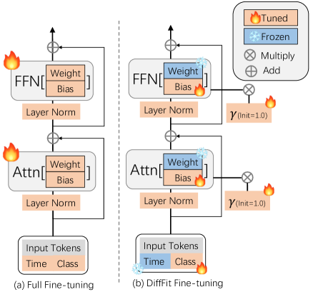
This section illustrates the integration of DiT with DiffFit. Note that DiffFit may be generalized to other diffusion models e.g. Stable Diffusion. Our approach, illustrated in Figure 4, involves freezing the majority of parameters in the latent diffusion model and training only the bias term, normalization, and class condition module. We moreover insert learnable scale factors into several blocks of the diffusion model, wherein the is initialized to 1.0 and multiplied on corresponding layers of each block. Each block typically contains multiple components such as multi-head self-attention, feed-forward networks, and layer normalization, and the block can be stacked times. Please refer to Algorithm 1 for additional detailed information.
| Food | SUN | DF-20M | Caltech | CUB-Bird | ArtBench | Oxford Flowers | Standard Cars | Average FID | Params. (M) | Train Time | |
| Full Fine-tuning | 10.46 | 7.96 | 17.26 | 35.25 | 5.68 | 25.31 | 21.05 | 9.79 | 16.59 | 673.8 (100%) | 1 |
| Adapt-Parallel [9] | 13.67 | 11.47 | 22.38 | 35.76 | 7.73 | 38.43 | 21.24 | 10.73 | 20.17 | 4.28 (0.63%) | 0.47 |
| Adapt-Sequential | 11.93 | 10.68 | 19.01 | 34.17 | 7.00 | 35.04 | 21.36 | 10.45 | 18.70 | 4.28 (0.63%) | 0.43 |
| BitFit [83] | 9.17 | 9.11 | 17.78 | 34.21 | 8.81 | 24.53 | 20.31 | 10.64 | 16.82 | 0.61 (0.09%) | 0.45 |
| VPT-Deep [31] | 18.47 | 14.54 | 32.89 | 42.78 | 17.29 | 40.74 | 25.59 | 22.12 | 26.80 | 2.81 (0.42%) | 0.50 |
| LoRA-R8 [30] | 33.75 | 32.53 | 120.25 | 86.05 | 56.03 | 80.99 | 164.13 | 76.24 | 81.25 | 1.15 (0.17%) | 0.63 |
| LoRA-R16 | 34.34 | 32.15 | 121.51 | 86.51 | 58.25 | 80.72 | 161.68 | 75.35 | 81.31 | 2.18 (0.32%) | 0.68 |
| DiffFit (ours) | 6.96 | 8.55 | 17.35 | 33.84 | 5.48 | 20.87 | 20.18 | 9.90 | 15.39 | 0.83 (0.12%) | 0.49 |
Fine-tuning.
During fine-tuning, diffusion model parameters are initially frozen, after which only specific parameters related to bias, class embedding, normalization, and scale factor are selectively unfrozen. Our approach, outlined in Algorithm 2, enables fast fine-tuning while minimizing disruption to pre-trained weights. DiT-XL/2 requires updating only 0.12% of its parameters, leading to training times approximately 2 faster than full fine-tuning. Our approach avoids catastrophic forgetting while reinforcing the pre-trained model’s knowledge and enabling adaptation to specific tasks.
Inference and Storage.
After fine-tuning on datasets, we only need to store one copy of the original model’s full parameters and dataset-specific trainable parameters, typically less than 1M for the latter. Combining these weights for the diffusion model enables adaptation to multiple domains for class-conditional image generation.
3.3 Analysis
In this subsection, we provide intuitive theoretical justifications for the efficacy of scaling factors and reveal the principle behind their effectiveness. We note that these theoretical justifications are intended as a simple proof of concept rather than seeking to be comprehensive, as our contributions are primarily experimental.
Specifically, recent theoretical works for diffusion models, such as [13, 12, 36, 8, 7], have shown that under suitable conditions on the data distribution and the assumption of approximately correct score matching, diffusion models can generate samples that approximately follow the data distribution, starting from a standard Gaussian distribution. Given a mapping and a distribution , we denote as a pushforward measure, i.e., for any measurable , we have . Note that our base model DiT is pre-trained on ImageNet with a resolution of and is fine-tuned on downstream datasets with the same resolution but much fewer data points and classes. Motivated by this, if assuming that the data in the ImageNet dataset follows a distribution , then we can assume that the data in the downstream dataset follows a distribution , where is a linear mapping dependent on some ground-truth scaling factors .
With these assumptions in place, we can formulate an intuitive theorem that provides insight into the effectiveness of scaling factors. A formal version of this theorem is included in the supplementary material.
Theorem 1 (informal).
Suppose that for a dataset generated from data distribution , we can train a neural network such that the diffusion model generates samples that approximately follow . Further assuming that the data distribution for a relatively small dataset can be written as with being a linear mapping dependent on ground-truth scaling factors . Then, if only re-training the neural network with the goal of optimizing scaling factors (and all other parameters remain unchanged), under suitable conditions, a simple gradient descent algorithm seeks an estimate that is close to with high probability. Furthermore, with the fine-tuned neural network corresponding to , the denoising process produces samples following a distribution that is close to .
In summary, Theorem 1 essentially states that when distributions and satisfy the condition that with being dependent on ground-truth scaling factors , diffusion models can transfer from distribution to in the denoising process with fine-tuning the scaling factors in the training process.
4 Experiments
4.1 Implementation Details
Our base model is the DiT111https://github.com/facebookresearch/DiT, which is pre-trained on ImageNet 256256 with 7 million iterations, achieving an FID score of 2.27222https://dl.fbaipublicfiles.com/DiT/models/DiT-XL-2-256x256.pt. However, since the original DiT repository does not provide training code, we re-implemented this and achieved reasonable results. Following DiT, we set the constant lr=1e-4 for full fine-tuning and set the classifier-free guidance to 1.5 for evaluation and 4.0 for visualization. In addition, we re-implemented several parameter-efficient fine-tuning methods such as Adaptor, BitFit, Visual Prompt Tuning (VPT), and LoRA. We found VPT to be sensitive to depth and token number while training was exceptionally unstable. As such, we sought for a more stable configuration with depth=5, token=1, and kept the final layers unfrozen for all tasks. We enlarge lr 10 for parameter-efficient fine-tuning settings to obtain better results following previous works [30, 9].
4.2 Transfer to Downstream Datasets
Setup.
For fine-tuning downstream small datasets with 256256 resolutions, we use 8 V100 GPUs with a total batch size of 256 and train 24K iterations. We choose 8 commonly used fine-grained datasets: Food101, SUN397, DF-20M mini, Caltech101, CUB-200-2011, ArtBench-10, Oxford Flowers and Stanford Cars. We report FID using 50 sampling steps for all the tasks. Most of these datasets are selected from CLIP downstream tasks except ArtBench-10 since it has distinct distribution from ImageNet, which enables a more comprehensive evaluation of the out-of-distribtion generalization performance of our DiffFit.
Results.
We list the performance of different parameter-efficient fine-tuning methods in Table 1. As can be seen, by tuning only parameters, our DiffFit achieves the lowest FID on average over downstream tasks. While full fine-tuning is a strong baseline and has slightly better results on 3/8 datasets, it is necessary to fine-tune 100% parameters. Among all baselines, the performance of LoRA is surprisingly poor. As discussed in [25], LoRA performs worse on image classification tasks than other parameter-efficient fine-tuning methods. As the image generation task is conceptually more challenging than the image classification task, it is reasonable that the performance gap between LoRA and other approaches becomes larger here.
| Method | FID | Training Cost (GPU days) |
| BigGAN-Deep [3] | 8.43 | 256-512 |
| StyleGAN-XL [64] | 2.41 | 400 |
| ADM-G, AMD-U [15] | 3.85 | 1914 |
| DiT-XL/2 [53] | 3.04 | 1733 |
| DiffFit (ours) | 3.02 | 51 (+950†) |
| Method | Pre-trained Checkpoint | FID |
| Full Fine-tune | IN256(7M)Food256 | 23.08 |
| DiffFit | IN512 (3M) | 19.25 |
| DiffFit | IN256 (7M)Food256 | 19.50 |
| +PosEnc Trick | IN256 (7M)Food256 | 19.10 |
| Blocks | #params (M) | FID |
| 2825 | 0.747 | 10.04 |
| 2822 | 0.754 | 10.03 |
| 2818 | 0.763 | 10.33 |
| 2814 | 0.770 | 10.51 |
| 2811 | 0.779 | 9.92 |
| 288 | 0.786 | 9.28 |
| 284 | 0.796 | 8.87 |
| 281 | 0.803 | 8.19 |
| Blocks | #params (M) | FID |
| 13 | 0.745 | 8.29 |
| 17 | 0.754 | 7.99 |
| 111 | 0.763 | 7.72 |
| 114 | 0.770 | 7.61 |
| 118 | 0.779 | 7.63 |
| 121 | 0.786 | 7.67 |
| 125 | 0.796 | 7.85 |
| 128 | 0.803 | 8.19 |
| #ID | Scale Factor | FID |
| 1 | NA (BitFit) | 9.17 |
| 2 | +Blocks | 8.19 |
| 3 | +PatchEmb | 9.05 |
| 4 | +TimeEmb | 8.46 |
| 5 | +QKV-Linear | 7.37 |
| 6 | +Final Layer | 7.49 |
| 7 | +ID 1, 2, 5, 6 | 7.17 |
| 8 | +(114 Layers) | 6.96 |
| LR Ratio | FID |
| 0.1 | 25.85 |
| 0.2 | 21.42 |
| 0.5 | 17.16 |
| 1 | 15.68 |
| 2 | 13.84 |
| 5 | 10.97 |
| 10 | 8.19 |
| 20 | 8.30 |
4.3 From Low Resolution to High Resolution
Setup.
Considering the generating images with different resolutions as a special type of distribution shift, our proposed method can effortlessly adapt a pre-trained low-resolution diffusion model to generate high-resolution images. To demonstrate the effectiveness of DiffFit, we load a pre-trained ImageNet DiT-XL/2 checkpoint and fine-tune the model on the ImageNet . We employ a positional encoding trick to speed up fine-tuning. We fine-tune DiT-XL/2 on ImageNet using 32 V100 GPUs with 1024 batch size and 30K iterations. We report FID using 250 sampling steps. Note that we do not need to fine-tune the label embedding here since the label does not change.
Positional Encoding Trick.
DiT [53] adopts a static sinusoidal 2D positional encoding scheme. To better utilize the positional information encoded in the pre-trained model, we develop a sinusoidal interpolation that aligns the positional encoding of 512512 resolution with that of 256256 resolution. This is implemented by replacing each pixel coordinate in the positional encoding formula with its half value , which is simple and have no extra costs.

Results.
As demonstrated in Table 2, DiffFit achieves 3.02 FID on the ImageNet benchmark, surpassing ADM’s 3.84 and the official DiT’s 3.04. DiffFit sets a new state-of-the-art among diffusion-based methods. Importantly, our method is significantly more efficient than the previous methods, as the fine-tuning process only requires an overhead of 51 GPU days. Even when accounting for the 950 GPU days of pre-training, our method remains superior to the 1500+ GPU days required by DiT and ADM. We observe faster training convergence using the positional encoding trick, as shown in Figure 5. For more visualizations please see Figure 1 and appendix.
In Table 3, we conducted fine-tuning experiments on the Food101 dataset with a resolution of 512512 using the DiffFit method. Our results reveal that fine-tuning a pre-trained Food101 256256 checkpoint with DiffFit yields a FID of 4 improvements over full fine-tuning. Interestingly, we found that utilizing a pre-trained ImageNet 512512 checkpoint leads to a FID performance similar to that achieved by the pre-trained Food101 with 256256 resolution. Moreover, we observed a slight improvement in FID performance by incorporating the proposed positional encoding trick into the fine-tuning process.
4.4 Fine-tuning Convergence Analysis
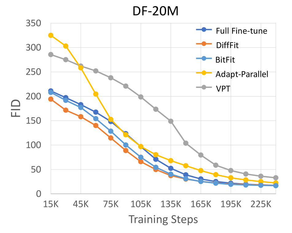
To facilitate the analysis of converging speed, we present the FID scores for several methods every 15,000 iterations in the Food-101, ArtBench-10, Flowers-102 and CUB-200 datasets, as shown in Figure 6. Our observations demonstrate that full fine-tuning, BitFit, and our proposed DiffFit exhibit similar convergence rates, which surpass the initial performance of AdaptFormer and VPT. While AdaptFormer initially presents inferior performance, it shows a rapid improvement in the middle of training. In contrast, VPT exhibits the slowest rate of convergence. Compared to full fine-tuning, DiffFit freezes most of the parameters and thus maximally preserves the information learned during the pre-training and thus achieves a better fine-tuned performance. Compared to BifFit, DiffFit adjusts the feature using scale factor, resulting in faster convergence and better results.
The above observation and analysis verify that our proposed DiffFit demonstrates fast adaptation abilities to target domains and an excellent image generation capability.
4.5 Ablation studies
Setup.
We conduct ablation studies on Food101 dataset, which has 101 classes. Each class has 750/250 images in the train/test set. Other settings are the same as Section 4.2.
Scale factor in different layers.
We investigate the effect of the scaling factor via 2 designs: gradually adding from deep to shallow (Table LABEL:tab:d2s) and from shallow to deep (Table LABEL:tab:s2d). The results demonstrate that adding before the 14th layer of DiT-XL/2 gradually increases the performance from 8.29 to 7.61 FID while adding more in the deeper layers hurts the performance. We hypothesize that deeper layers are responsible for learning high-level features that capture abstract data patterns, which contribute to synthesizing the final output and are often complex and non-linear. Adding in deeper layers poses a risk of disrupting the learned correlations between the high-level features and data, which might negatively impact the model.
Scale factor in different modules.
We study the impact of scaling factor in various DiT modules, as illustrated in Table LABEL:tab:scale_location. Based on BitFit [83]’s FID score of 9.17, incorporating the scaling factor in transformer blocks and QKV-linear layers of self-attention can significantly enhance the performance, resulting in a FID score of 7.37 (row 5). However, introducing scale factors in other modules, such as patch embedding (row 3) and time embedding (row 4), does not bring noticeable improvements. By integrating the effective designs, i.e., adding in blocks, QKV-linear and final layers, we improve FID score to 7.17 (row 7). We further improve the FID score of 6.96 by placing in the first 14 blocks (Table LABEL:tab:s2d). This optimal setting is adopted as the final setting for our approach.
Learning rate.
Adjusting the learning rate is a crucial step in fine-tuning. Parameter-efficient fine-tuning typically requires a larger learning rate than the pre-training [30, 9] since pre-training has already initialized most of the model’s parameters to a certain extent and a larger learning rate can help quickly adapt the remaining parameters to the new tasks. We perform a learning rate search on our method, as shown in Table LABEL:tab:lr. We observe that using a learning rate 10 greater than pre-training yields the best result. Larger learning rates than 10 resulted in decreased performance and even unstable training.
5 Conclusions and Limitations
In this paper, we propose DiffFit, a straightforward yet effective fine-tuning approach that can quickly adapt a large pre-trained diffusion model to various downstream domains, including different datasets or varying resolutions. By only fine-tuning bias terms and scaling factors, DiffFit provides a cost-effective solution to reduce storage requirements and speed up fine-tuning without compromising performance. One limitation is that our experiments mainly focus on class-conditioned image generation. It is still unclear whether this strategy could perform equally well in more complex tasks such as text-to-image generation or video/3D generation. We leave these areas for future research.
Acknowledgement.
We would like to express our gratitude to Junsong Chen, Chongjian Ge, and Jincheng Yu for their assistance with experiments on LLaMA and DreamBooth.
Supplementary Material
DiffFit: Unlocking Transferability of Large Diffusion Models
via Simple Parameter-efficient Fine-Tuning
6 More Applications
6.1 Combine DiffFit with ControlNet
Setup.
To verify that DiffFit can be applied to large-scale text-to-image generation models, we conducted experiments on the recent popular ControlNet [84] model. We used the official code of ControlNet333https://github.com/lllyasviel/ControlNet, and chose the semantic segmentation mask as the additional condition. We used the COCO-Stuff [5] as our dataset and the text prompt was generated by the BLIP [38]. The model was trained on the training set and evaluated on the validation set using 8 V100 GPUs with a batch size of 2 per GPU and 20 epochs. Unless otherwise stated, we followed the official implementation of ControlNet for all hyper-parameters including the learning rate and the resolution.
Combination.
ControlNet [84] enhances the original Stable Diffusion (SD) by incorporating a conditioning network comprising two parts: a set of zero convolutional layers initialized to zero and a trainable copy of 13 layers of SD initialized from a pre-trained model.
In our DiffFit setting, we freeze the entire trainable copy part and introduce a scale factor of in each layer. Then, we unfreeze the and all the bias terms. Note that in ControlNet, the zero convolutional layers are required to be trainable. Table 5 shows that DiffFit has 11.2M trainable parameters while the zero convolutional layers contribute 10.8M parameters. Reducing the trainable parameters in zero convolutional layers is plausible, but it is beyond the scope of this paper.
Results.
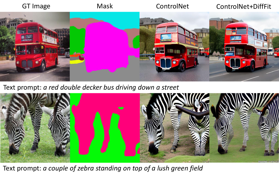
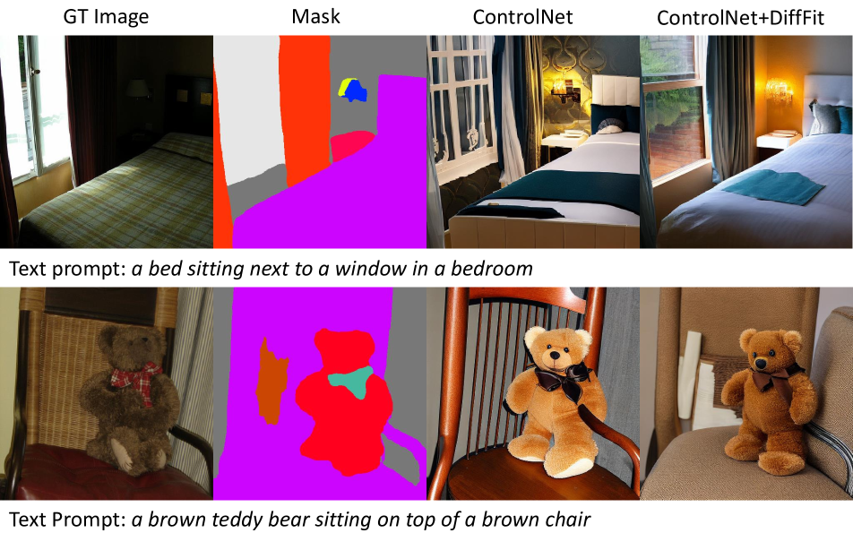
Table 5 displays the results obtained from the original ControlNet and the results from combining DiffFit with ControlNet. Our results show that the addition of DiffFit leads to comparable FID and CLIP scores while significantly reducing the number of trainable parameters. In addition, we note that ControlNet primarily focuses on fine-grained controllable generation while FID and CLIP score may not accurately reflect the overall performance of a model. Figures 7 and 8 compare the results from ControlNet and DiffFit. When using the same mask and text prompt as conditions, fine-tuning with DiffFit produces more visually appealing results compared to fine-tuning with the original ControlNet.
Our experimental results suggest that DiffFit has great potential to improve the training of other types of advanced generative models.
6.2 Combine DiffFit with DreamBooth
Setup.
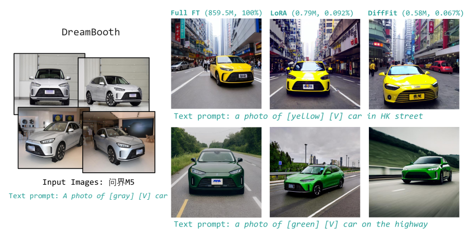
Our DiffFit can also be easily combined with the DreamBooth [61]. DreamBooth is a personalized text-to-image diffusion model that fine-tunes a pre-trained text-to-image model using a few reference images of a specific subject, allowing it to synthesize fully-novel photorealistic images of the subject contextualized in different scenes. Our implementation on DreamBooth utilizes the codebase from Diffusers444https://github.com/huggingface/diffusers/tree/main/examples/dreambooth, with Stable Diffusion as the base text-to-image model.
Implementation detail.
Given 3-5 input images, the original DreamBooth fine-tunes the subject embedding and the entire text-to-image (T2I) model. In contrast, our DiffFit simplifies the fine-tuning process by incorporating scale factor into all attention layers of the model and requiring only the , bias term, LN, and subject embedding to be fine-tuned.
Results.
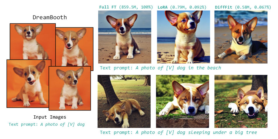
We compare the original full-finetuning approach of DreamBooth with the fine-tuning using LoRA and DiffFit, as shown in Figures 9 and 10. First, we observe that all three methods produce similar generation quality. Second, we find that the original full-finetuning approach is storage-intensive, requiring the storage of 859M parameters for one subject-driven fine-tuning. In contrast, LoRA and DiffFit are both parameter-efficient (requiring the storage of less than 1% parameters), with DiffFit further reducing trainable parameters by about 26% compared to LoRA.
6.3 Combine DiffFit with LLaMA and Alpaca
Setup.
LLaMA [72] is an open and efficient large language model (LLM) from Meta, ranging from 7B to 65B parameters. Alpaca is a model fully fine-tuned from the LLaMA 7B model on 52K instruction-following demonstrations and behaves qualitatively similarly to OpenAI’s ChatGPT model text-davinci-003.
Combination.
We use the original code from Alpaca555https://github.com/tatsu-lab/stanford_alpaca as the baseline and compare it with Alpaca-LoRA666https://github.com/tloen/alpaca-lora. Since LLaMA and DiT have a similar Transformer design, the fine-tuning strategy of LLaMA-DiffFit is exactly the same as that of DiT-DiffFit, except that the learning rate is set to 3e-4 to align with Alpaca-LoRA.
Results.
In Table 6, we showcase the instruction tuning results on llama using Alpaca, LoRA, and DiffFit. The trainable parameters of Alpaca, LoRA, and DiffFit are 7B, 6.7M, and 0.7M. The model fine-tuned with DiffFit exhibits strong performance in natural language question-answering tasks (e.g., common sense questioning, programming, etc.). This validates the efficacy of DiffFit for instruction tuning in NLP models, highlighting DiffFit as a flexible and general fine-tuning approach.
| Method | FID | CLIP Score | Total Params (M) | Trainable Params (M) |
| ControlNet | 20.1 | 0.3067 | 1343 | 361 |
| ControlNet + DiffFit | 19.5 | 0.3064 | 1343 | 11.2 |
| Instruction: Tell me about alpacas. Alpaca: Alpacas are small, fluffy animals related to camels and llamas. They are native to Peru and Bolivia, and were first domesticated around 5,000 years ago. They are kept mainly for their fine, soft fleece, which is used to make knitwear and other garments. Alpacas are herd animals and live in small family groups, led by an older male. They are highly social animals and can form strong bonds with their owners. Alpaca-LoRA: Alpacas are members of the camelid family and are native to the Andes Mountains of South America. They are known for their soft, luxurious fleece, which is used to make clothing, blankets, and other items. Alpacas are herbivores and graze on grasses and other plants. They are social animals and live in herds of up to 20 individuals. LLaMA-DiffFit: Alpacas are members of the camelid family and are native to the Andes Mountains in South America. They are domesticated for their soft, luxurious fleece, which is used to make clothing, blankets, and other textiles. Alpacas are herbivores and graze on grasses and other plants. They can live up to 20 years in captivity and are known for their gentle nature. Instruction: List all Canadian provinces in alphabetical order. Alpaca: Alberta, British Columbia, Manitoba, New Brunswick, Newfoundland and Labrador, Nova Scotia, Ontario, Prince Edward Island, Quebec, Saskatchewan, Northwest Territories, Nunavut, Yukon. Alpaca-LoRA: Alberta, British Columbia, Manitoba, New Brunswick, Newfoundland and Labrador, Nova Scotia, Ontario, Prince Edward Island, Quebec, Saskatchewan. LLaMA-DiffFit: Alberta, British Columbia, Manitoba, New Brunswick, Newfoundland and Labrador, Northwest Territories, Nova Scotia, Nunavut, Ontario, Prince Edward Island, Quebec, Saskatchewan, Yukon. Instruction: Tell me five words that rhyme with ’shock’. Alpaca: Five words that rhyme with shock are: rock, pop, shock, cook, and snock. Alpaca-LoRA: Flock, lock, rock, stock, and sock. LLaMA-DiffFit: Shock, sock, rock, cook, and book. Instruction: Write a Python program that prints the first 10 Fibonacci numbers. Alpaca: ⬇ numbers = [0, 1] for i in range(2, 11): numbers.append(numbers[i-2] + numbers[i-1]) print(numbers) # Output: [0, 1, 1, 2, 3, 5, 8, 13, 21, 34] Alpaca-LoRA: ⬇ def fibonacci(n): if n == 0: return 0 elif n == 1: return 1 else: return fibonacci(n-1) + fibonacci(n-2) print(fibonacci(10)) LLaMA-DiffFit: ⬇ def fib(n): if n == 0: return 0 elif n == 1: return 1 else: return fib(n-1) + fib(n-2) print(fib(10)) |
7 More Implementation Details
7.1 Adding the Scale Factor in Self-Attention
This section demonstrates the incorporation of scale factor into the self-attention modules. Traditionally, a self-attention layer comprises two linear operations: (1) QKV-Linear operation and (2) Project-Linear operation. Consistent with the approach discussed above in the paper, the learnable scale factor is initialized to 1.0 and subsequently fine-tuned. Algorithm 3 presents the Pytorch-style pseudo code.
7.2 Dataset Description
This section describes 8 downstream datasets/tasks that we have utilized in our experiments to fine-tune the DiT with our DiffFit method.
Food101 [2].
This dataset contains 101 food categories, totaling 101,000 images. Each category includes 750 training images and 250 manually reviewed test images. The training images were kept intentionally uncleaned, preserving some degree of noise, primarily vivid colors and occasionally incorrect labels. All images have been adjusted to a maximum side length of 512 pixels.
SUN 397 [79].
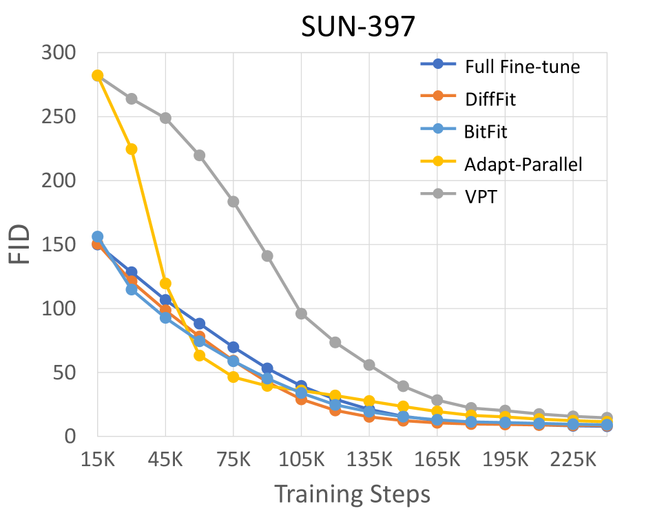
The SUN benchmark database comprises 108,753 images labeled into 397 distinct categories. The quantities of images vary among the categories, however, each category is represented by a minimum of 100 images. These images are commonly used in scene understanding applications.
DF20M [54].
DF20 is a new fine-grained dataset and benchmark featuring highly accurate class labels based on the taxonomy of observations submitted to the Danish Fungal Atlas. The dataset has a well-defined class hierarchy and a rich observational metadata. It is characterized by a highly imbalanced long-tailed class distribution and a negligible error rate. Importantly, DF20 has no intersection with ImageNet, ensuring unbiased comparison of models fine-tuned from ImageNet checkpoints.
Caltech 101 [22].
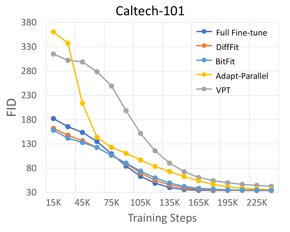
The Caltech 101 dataset comprises photos of objects within 101 distinct categories, with roughly 40 to 800 images allocated to each category. The majority of the categories have around 50 images. Each image is approximately 300200 pixels in size.
CUB-200-2011 [76].
CUB-200-2011 (Caltech-UCSD Birds-200-2011) is an expansion of the CUB-200 dataset by approximately doubling the number of images per category and adding new annotations for part locations. The dataset consists of 11,788 images divided into 200 categories.
ArtBench-10 [43].
ArtBench-10 is a class-balanced, standardized dataset comprising 60,000 high-quality images of artwork annotated with clean and precise labels. It offers several advantages over previous artwork datasets including balanced class distribution, high-quality images, and standardized data collection and pre-processing procedures. It contains 5,000 training images and 1,000 testing images per style.
Oxford Flowers [51].
The Oxford 102 Flowers Dataset contains high quality images of 102 commonly occurring flower categories in the United Kingdom. The number of images per category range between 40 and 258. This extensive dataset provides an excellent resource for various computer vision applications, especially those focused on flower recognition and classification.
Stanford Cars [35].
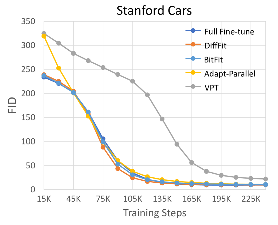
In the Stanford Cars dataset, there are 16,185 images that display 196 distinct classes of cars. These images are divided into a training and a testing set: 8,144 images for training and 8,041 images for testing. The distribution of samples among classes is almost balanced. Each class represents a specific make, model, and year combination, e.g., the 2012 Tesla Model S or the 2012 BMW M3 coupe.
8 More FID Curves
We present additional FID curves for the following datasets: Stanford Cars, SUN 397, Caltech 101, and DF20M as illustrated in Figures 12 through 14, respectively. The results demonstrate that our DiffFit achieves rapid convergence, delivers compelling FID scores compared to other parameter-efficient finetuning strategies, and is competitive in the full-finetuning setting.
9 More Theoretical Analysis
In this section, we will provide a more detailed analysis of the effect of scaling factors. Specifically, we will present a formal version and proof of Theorem 1, which was informally stated in the main document.
Our theoretical results are closely related to the learning of neural networks. It is worth noting that the majority of works in this area concentrate on the simplified setting where the neural network only has one non-linearly activated hidden layer with no bias terms, see, e.g., [88, 21, 17, 85, 20, 74]. As our contributions are mainly experimental, we only provide some intuitive theoretical analysis to reveal the effect of scaling factors. To this end, we will consider the following simplified settings.
-
•
Following the approach of [33, 10], we replace the noise neural network used in the diffusion model with ,777Here we assume that in the forward process, the conditional distribution . See Section 3.1 in the main document. where is a neural network that approximates the original signal. In addition, in the sampling process, we assume a single sampling step from the end time to the initial time , which gives . For brevity, we denote by , and we assume that for all , where is a weight matrix, is the offset vector, and represents a non-linear activation function that does not grow super-linearly (cf. Appendix 9.3) and it is applied element-wise. While one-step generation may seem restrictive, recent works [44, 65] have achieved it for the diffusion models.
-
•
Suppose that we have a dataset generated from distribution . Further assuming that there exist ground-truth scaling factors such that each entry of any data point in a relatively small dataset generated from distribution can be written as for some sampled from . We denote this transition from to as for brevity.
- •
Under the above settings, in the training process for the diffusion model using the relatively small dataset, if we only fine-tune the scaling factors, the objective function can be expressed as:
| (2) |
where , (then corresponds to an entry of data point generated from ), and is the number of training samples. As is sub-Gaussian (cf. Appendix 9.2) and with being close to , we assume that can be represented as , where each entry of is zero-mean sub-Gaussian with the sub-Gaussian norm (cf. Appendix 9.2 for the definition of sub-Gaussian norm) being upper bounded by some small constant .
Let . We write , , and with . Then, we have and the objective function (2) can be re-written as
| (3) |
Let with , where is the -th entry of the offset vector and is the -th row of the weight matrix . Then, we have the following theorem concerning the optimal solution to (3). The proof of Theorem 2 is deferred to Section 9.4.
Theorem 2.
Under the above settings, if is an optimal solution to (3) and , with probability , it holds that
| (4) |
Note that is considered to be small and is a fixed positive constant. In addition, the gradient descent algorithm aims to minimize (3). Therefore, Theorem 2 essentially says that when the number of training samples is sufficiently large, the simple gradient descent algorithm finds an estimate that is close to with high probability (in the sense that the relative distance is small). Furthermore, with this , the diffusion model generates distribution , which is naturally considered to be close to since is close to and is close to .
9.1 Notation
We write for a positive integer . The unit sphere in is denoted by . We use to denote the spectral norm of a matrix . We use the symbols to denote absolute constants, whose values may differ from line to line.
9.2 General Auxiliary Results
First, the widely-used notion of an -net is presented as follows, see, e.g., [46, Definition 3].
Definition 1.
Let be a metric space, and fix . A subset is said be an -net of if, for all , there exists some such that . The minimal cardinality of an -net of , if finite, is denoted and is called the covering number of (at scale ).
The following lemma provides a useful bound for the covering number of the unit sphere.
Lemma 1.
[75, Lemma 5.2] The unit Euclidean sphere equipped with the Euclidean metric satisfies for every that
| (5) |
In addition, we have the following lemma concerning the spectral norm of a matrix.
Lemma 2.
[75, Lemma 5.3] Let be an matrix, and let be an -net of for some . Then
| (6) |
Standard definitions for sub-Gaussian and sub-exponential random variables are presented as follows.
Definition 2.
A random variable is said to be sub-Gaussian if there exists a positive constant such that for all , and the corresponding sub-Gaussian norm is defined as .
Definition 3.
A random variable is said to be sub-exponential if there exists a positive constant such that for all , and the corresponding sub-exponential norm is defined as .
The following lemma concerns the relation between sub-Gaussian and sub-exponential random variables.
Lemma 3.
[75, Lemma 5.14] A random variable is sub-Gaussian if and only if is sub-exponential. Moreover,
| (7) |
The following lemma provides a useful concentration inequality for the sum of independent sub-exponential random variables.
Lemma 4.
[75, Proposition 5.16] Let be independent zero-mean sub-exponential random variables, and . Then for every and , it holds that
| (8) |
where is an absolute constant. In particular, with , we have
| (9) |
9.3 Useful Lemmas
Throughout the following, we use to denote some non-linear activation function that does not grow faster than linear, i.e., there exist scalars and such that for all . Then, if is a random Gaussian variable, will be sub-Gaussian [48]. Note that the condition that does not grow super-linearly is satisfied by popular activation functions such as ReLU, Sigmoid, and Hyperbolic tangent function.
Lemma 5.
For , let be a random Gaussian variable. Then for every , we have
| (10) |
where and are dependent on and the non-linear activation function .
Proof.
We have
| (11) | ||||
| (12) | ||||
| (13) | ||||
| (14) |
In addition, from (12), by the Cauchy-Schwarz Inequality, we obtain
| (15) | ||||
| (16) |
This completes the proof. ∎
Lemma 6.
Let be a standard Gaussian matrix, i.e., each entry of is sampled from standard Gaussian distribution, and let be a fixed matrix that has no zero rows. In addition, for a fixed vector , let . Then, when , with probability , it holds that
| (17) |
where is an absolute constant and the non-linear activation function is applied element-wise.
Proof.
Let be the -th row of . By the assumption that has no zero rows, we have for all . Let . Then the -th entry of , denoted , follows the distribution. For any and any fixed , from Lemma 3, we obtain that is sub-exponential with the sub-exponential norm being upper bounded by , where is some absolute constant. Let be the expectation of . From Lemma 5, we obtain that it holds uniformly for all that
| (18) |
where is an absolute constant. In addition, from Lemma 4, for any , we obtain
| (19) |
From Lemma 1, there exists an -net of with . Taking a union bound over , we have that when , with probability , it holds for all that
| (20) |
Then, since (18) holds uniformly for all , setting , Lemma 2 implies that when , with probability ,
| (21) | ||||
| (22) | ||||
| (23) |
∎
Lemma 7.
Let us use the same notation as in Lemma 6. When , with probability , it holds for all that
| (24) |
where with .
Proof.
It suffices to consider the case that . From (20), we have that when , with probability , it holds for all that
| (25) |
In addition, from Lemma 5, we have that it hold uniformly for all that
| (26) |
Then, if setting for some small absolute constant , we have that when , with probability , for all ,
| (27) |
For any , there exists an such that , and thus
| (28) | ||||
| (29) | ||||
| (30) |
where (30) follows from Lemma 6 and the setting . Then, if is set to be sufficiently small, from (26), we have for all that
| (31) |
∎
Lemma 8.
Let be a matrix with independent zero-mean sub-Gaussian entries. Suppose that the sub-Gaussian norm of all entries of is upper bounded by some . Then, for any , we have that with probability ,
| (32) |
Proof.
Let be the -th row of . From the definition of sub-Gaussian norm, we have that if a random variable is zero-mean sub-Gaussian with , then
| (33) |
which implies
| (34) |
Then, we have
| (35) |
In addition, from Lemma 3, we also have that is sub-exponential with the sub-exponential norm being upper bounded by . Then, from Lemma 4, we obtain that for any , with probability ,
| (36) |
which implies
| (37) |
where the last inequality follows from (34). Setting , we obtain the desired result. ∎
9.4 Proof of Theorem 2
10 More Visualization Results
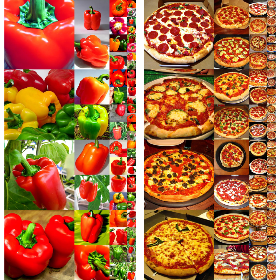
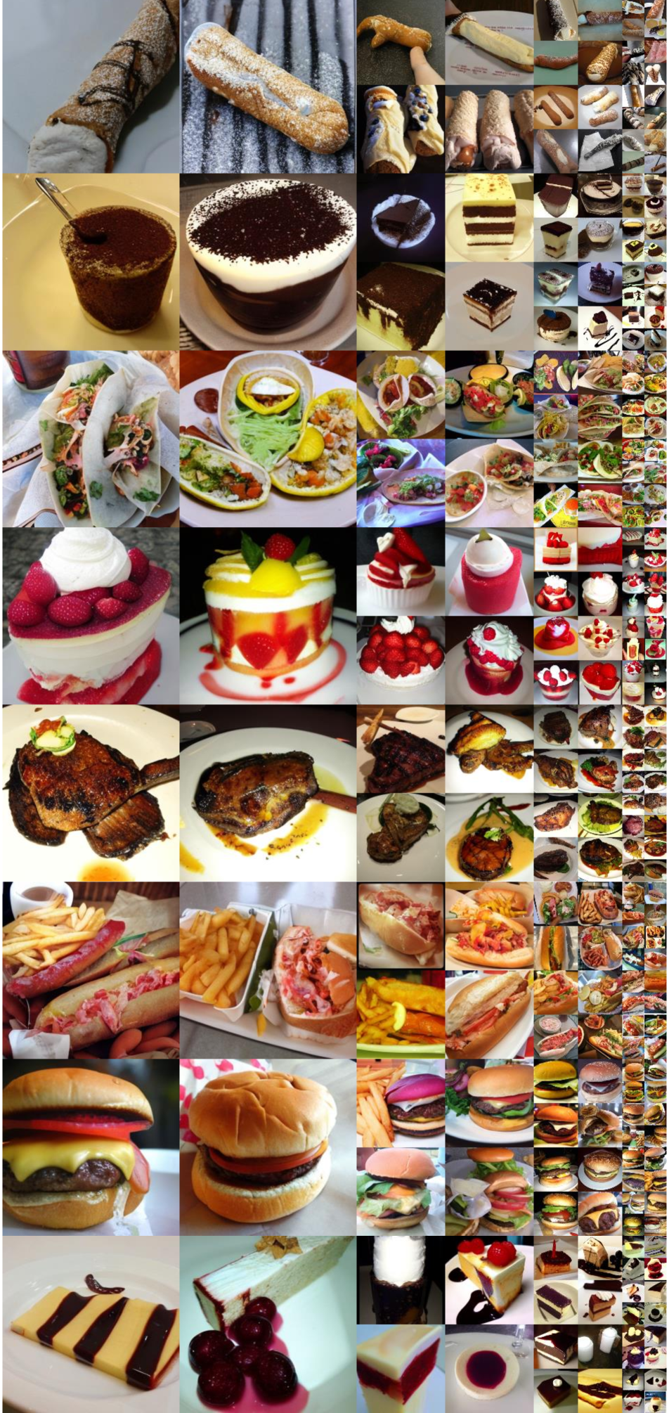
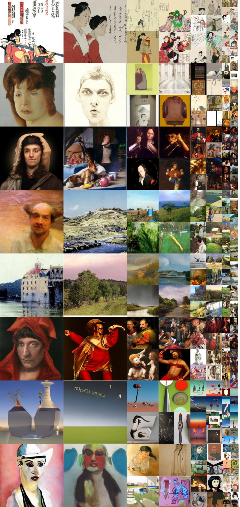
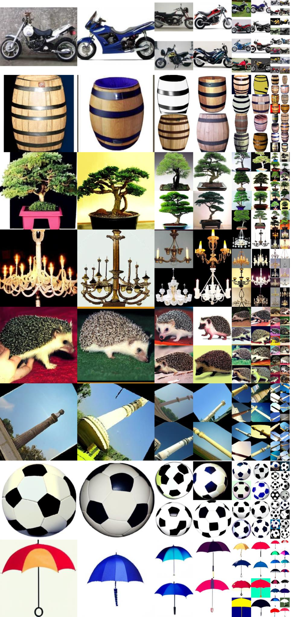
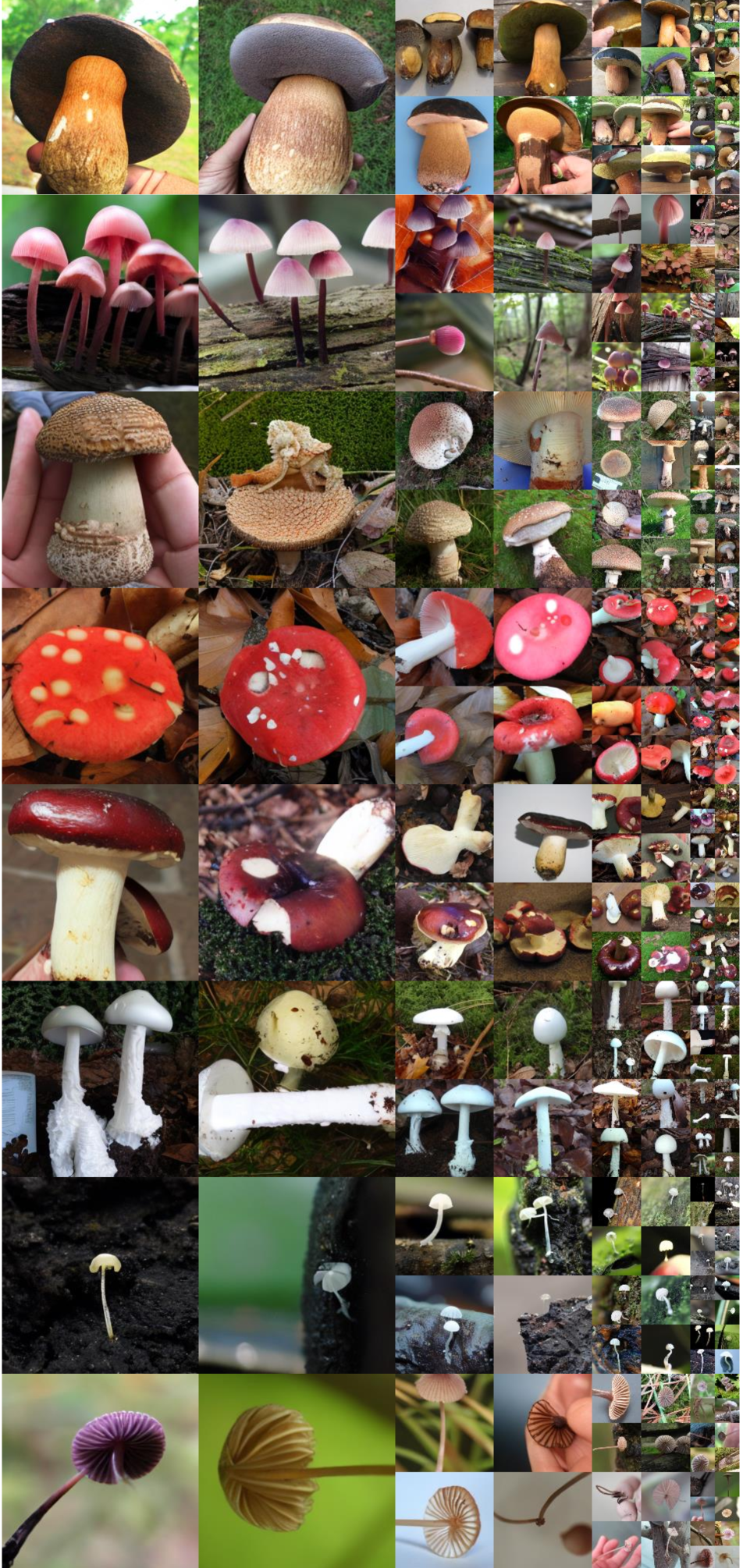
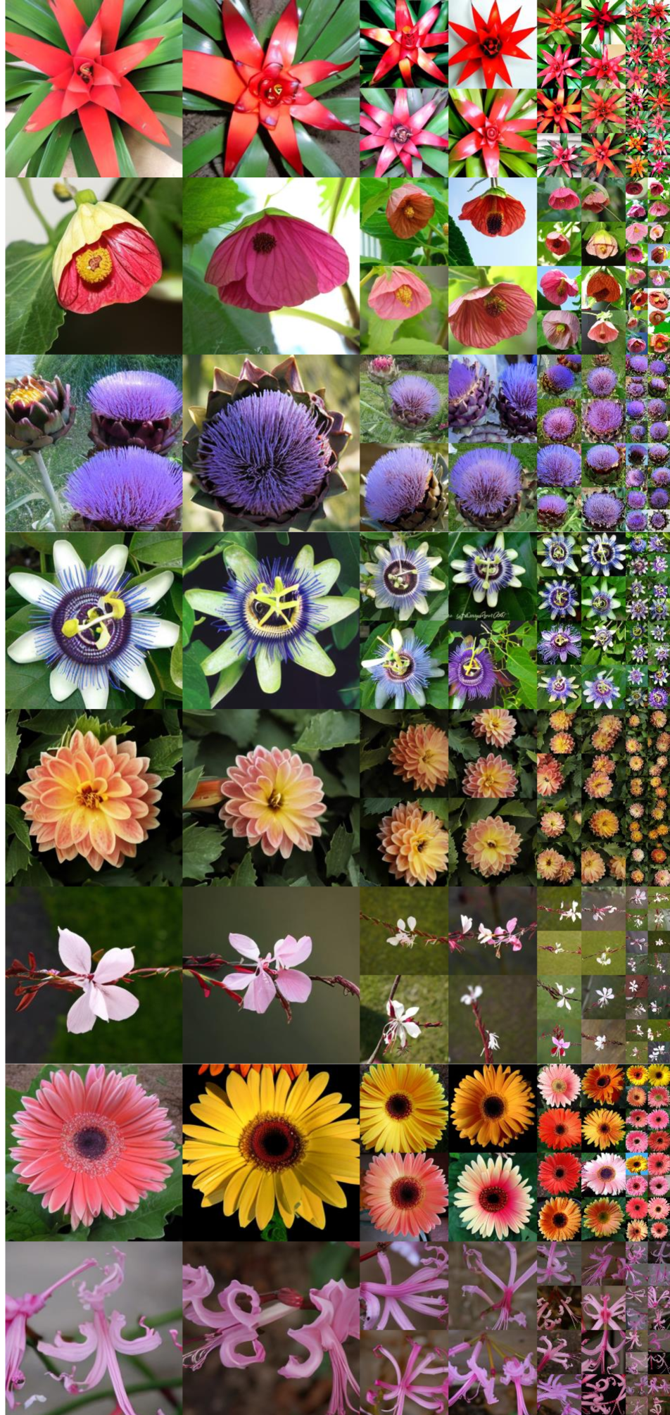
In this section, we present additional samples generated by the DiT-XL/2 + DiffFit fine-tuning. Specifically, we demonstrate its efficacy by generating high-quality images with a resolution of 512512 on the ImageNet dataset, as illustrated in Figures 15, 16, and 17. Additionally, we showcase the model’s capability on 8 downstream tasks by displaying its image generation results with a resolution of 256256, as depicted in Figures 19 through 25.
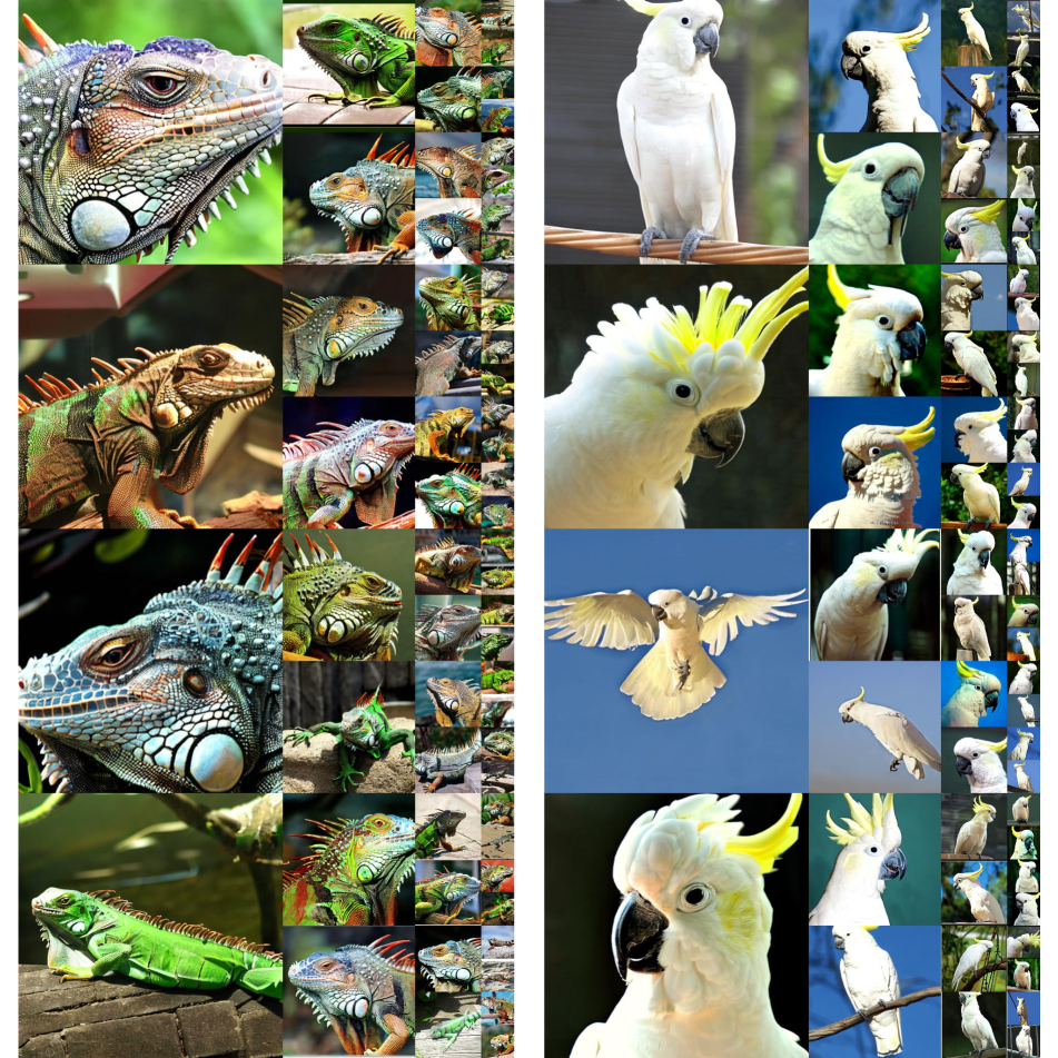

Classifier-free guidance scale = 4.0, sampling steps = 250.
Classifier-free guidance scale = 4.0, sampling steps = 250.

Classifier-free guidance scale = 4.0, sampling steps = 250.
Classifier-free guidance scale = 4.0, sampling steps = 250.
Classifier-free guidance scale = 4.0, sampling steps = 250.
Classifier-free guidance scale = 4.0, sampling steps = 250.
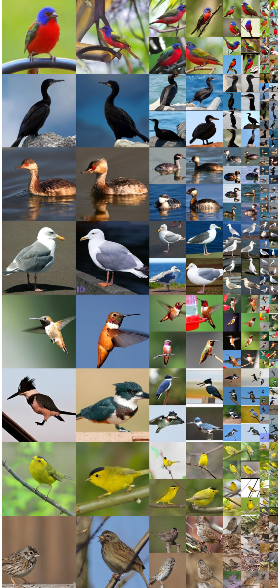
Classifier-free guidance scale = 4.0, sampling steps = 250.
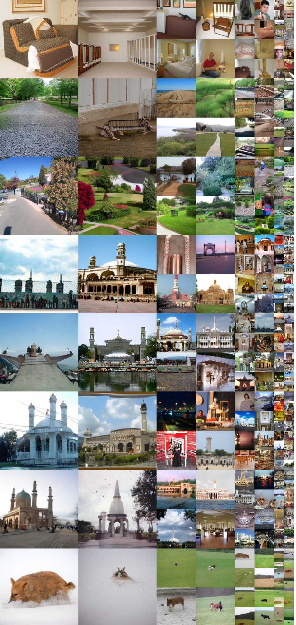
Classifier-free guidance scale = 4.0, sampling steps = 250.
References
- [1] Yogesh Balaji, Seungjun Nah, Xun Huang, Arash Vahdat, Jiaming Song, Karsten Kreis, Miika Aittala, Timo Aila, Samuli Laine, Bryan Catanzaro, et al. ediffi: Text-to-image diffusion models with an ensemble of expert denoisers. arXiv, 2022.
- [2] Lukas Bossard, Matthieu Guillaumin, and Luc Van Gool. Food-101–mining discriminative components with random forests. In ECCV, 2014.
- [3] Andrew Brock, Jeff Donahue, and Karen Simonyan. Large scale gan training for high fidelity natural image synthesis. arXiv, 2018.
- [4] Tom Brown, Benjamin Mann, Nick Ryder, Melanie Subbiah, Jared D Kaplan, Prafulla Dhariwal, Arvind Neelakantan, Pranav Shyam, Girish Sastry, Amanda Askell, et al. Language models are few-shot learners. NeurIPS, 2020.
- [5] Holger Caesar, Jasper Uijlings, and Vittorio Ferrari. Coco-stuff: Thing and stuff classes in context. In CVPR, 2018.
- [6] Nicolas Carion, Francisco Massa, Gabriel Synnaeve, Nicolas Usunier, Alexander Kirillov, and Sergey Zagoruyko. End-to-end object detection with transformers. In ECCV, 2020.
- [7] Minshuo Chen, Kaixuan Huang, Tuo Zhao, and Mengdi Wang. Score approximation, estimation and distribution recovery of diffusion models on low-dimensional data. arxiv, 2023.
- [8] Sitan Chen, Sinho Chewi, Jerry Li, Yuanzhi Li, Adil Salim, and Anru R Zhang. Sampling is as easy as learning the score: theory for diffusion models with minimal data assumptions. In ICLR, 2023.
- [9] Shoufa Chen, Chongjian Ge, Zhan Tong, Jiangliu Wang, Yibing Song, Jue Wang, and Ping Luo. Adaptformer: Adapting vision transformers for scalable visual recognition. arXiv, 2022.
- [10] Ting Chen, Ruixiang Zhang, and Geoffrey Hinton. Analog bits: Generating discrete data using diffusion models with self-conditioning. In ICLR, 2023.
- [11] Antonia Creswell, Tom White, Vincent Dumoulin, Kai Arulkumaran, Biswa Sengupta, and Anil A Bharath. Generative adversarial networks: An overview. IEEE signal processing magazine, 2018.
- [12] Valentin De Bortoli. Convergence of denoising diffusion models under the manifold hypothesis. TMLR, 2022.
- [13] Valentin De Bortoli, James Thornton, Jeremy Heng, and Arnaud Doucet. Diffusion schrödinger bridge with applications to score-based generative modeling. In NeurIPS, 2021.
- [14] Mostafa Dehghani, Josip Djolonga, Basil Mustafa, Piotr Padlewski, Jonathan Heek, Justin Gilmer, Andreas Steiner, Mathilde Caron, Robert Geirhos, Ibrahim Alabdulmohsin, et al. Scaling vision transformers to 22 billion parameters. arXiv, 2023.
- [15] Prafulla Dhariwal and Alexander Nichol. Diffusion models beat gans on image synthesis. NeurIPS, 2021.
- [16] Alexey Dosovitskiy, Lucas Beyer, Alexander Kolesnikov, Dirk Weissenborn, Xiaohua Zhai, Thomas Unterthiner, Mostafa Dehghani, Matthias Minderer, Georg Heigold, Sylvain Gelly, et al. An image is worth 16x16 words: Transformers for image recognition at scale. arXiv, 2020.
- [17] Simon S Du, Xiyu Zhai, Barnabas Poczos, and Aarti Singh. Gradient descent provably optimizes over-parameterized neural networks. In ICLR, 2019.
- [18] Patrick Esser, Robin Rombach, and Bjorn Ommer. Taming transformers for high-resolution image synthesis. In CVPR, 2021.
- [19] William Fedus, Barret Zoph, and Noam Shazeer. Switch transformers: Scaling to trillion parameter models with simple and efficient sparsity. JMLR, 2021.
- [20] Weihao Gao, Ashok V Makkuva, Sewoong Oh, and Pramod Viswanath. Learning one-hidden-layer neural networks under general input distributions. In AISTATS, 2019.
- [21] Rong Ge, Jason D Lee, and Tengyu Ma. Learning one-hidden-layer neural networks with landscape design. In ICLR, 2018.
- [22] Gregory Griffin, Alex Holub, and Pietro Perona. Caltech-256 object category dataset. 2007.
- [23] Kai Han, An Xiao, Enhua Wu, Jianyuan Guo, Chunjing Xu, and Yunhe Wang. Transformer in transformer. NeurIPS, 2021.
- [24] Kaiming He, Xinlei Chen, Saining Xie, Yanghao Li, Piotr Dollár, and Ross Girshick. Masked autoencoders are scalable vision learners. In CVPR, 2022.
- [25] Xuehai He, Chunyuan Li, Pengchuan Zhang, Jianwei Yang, and Xin Eric Wang. Parameter-efficient fine-tuning for vision transformers. arXiv, 2022.
- [26] Jonathan Ho, William Chan, Chitwan Saharia, Jay Whang, Ruiqi Gao, Alexey Gritsenko, Diederik P Kingma, Ben Poole, Mohammad Norouzi, David J Fleet, et al. Imagen video: High definition video generation with diffusion models. arXiv, 2022.
- [27] Jonathan Ho, Ajay Jain, and Pieter Abbeel. Denoising diffusion probabilistic models. NeurIPS, 2020.
- [28] Jonathan Ho, Tim Salimans, Alexey Gritsenko, William Chan, Mohammad Norouzi, and David J Fleet. Video diffusion models. arXiv, 2022.
- [29] Neil Houlsby, Andrei Giurgiu, Stanislaw Jastrzebski, Bruna Morrone, Quentin De Laroussilhe, Andrea Gesmundo, Mona Attariyan, and Sylvain Gelly. Parameter-efficient transfer learning for nlp. In ICML, 2019.
- [30] Edward J Hu, Yelong Shen, Phillip Wallis, Zeyuan Allen-Zhu, Yuanzhi Li, Shean Wang, Lu Wang, and Weizhu Chen. Lora: Low-rank adaptation of large language models. arxiv, 2021.
- [31] Menglin Jia, Luming Tang, Bor-Chun Chen, Claire Cardie, Serge Belongie, Bharath Hariharan, and Ser-Nam Lim. Visual prompt tuning. In ECCV, 2022.
- [32] Yifan Jiang, Shiyu Chang, and Zhangyang Wang. Transgan: Two pure transformers can make one strong gan, and that can scale up. NeurIPS, 2021.
- [33] Diederik Kingma, Tim Salimans, Ben Poole, and Jonathan Ho. Variational diffusion models. NeurIPS, 2021.
- [34] Diederik P Kingma, Max Welling, et al. An introduction to variational autoencoders. Foundations and Trends® in Machine Learning, 2019.
- [35] Jonathan Krause, Michael Stark, Jia Deng, and Li Fei-Fei. 3d object representations for fine-grained categorization. In ICCV workshops, 2013.
- [36] Holden Lee, Jianfeng Lu, and Yixin Tan. Convergence for score-based generative modeling with polynomial complexity. In NeurIPS, 2022.
- [37] Brian Lester, Rami Al-Rfou, and Noah Constant. The power of scale for parameter-efficient prompt tuning. arXiv, 2021.
- [38] Junnan Li, Dongxu Li, Caiming Xiong, and Steven Hoi. Blip: Bootstrapping language-image pre-training for unified vision-language understanding and generation. In ICML, 2022.
- [39] Xiang Lisa Li and Percy Liang. Prefix-tuning: Optimizing continuous prompts for generation. arXiv, 2021.
- [40] Zhiqi Li, Wenhai Wang, Hongyang Li, Enze Xie, Chonghao Sima, Tong Lu, Yu Qiao, and Jifeng Dai. Bevformer: Learning bird’s-eye-view representation from multi-camera images via spatiotemporal transformers. In ECCV, 2022.
- [41] Zhiqi Li, Wenhai Wang, Enze Xie, Zhiding Yu, Anima Anandkumar, Jose M Alvarez, Ping Luo, and Tong Lu. Panoptic segformer: Delving deeper into panoptic segmentation with transformers. In CVPR, 2022.
- [42] Dongze Lian, Daquan Zhou, Jiashi Feng, and Xinchao Wang. Scaling & shifting your features: A new baseline for efficient model tuning. arXiv, 2022.
- [43] Peiyuan Liao, Xiuyu Li, Xihui Liu, and Kurt Keutzer. The artbench dataset: Benchmarking generative models with artworks. arXiv, 2022.
- [44] Xingchao Liu, Chengyue Gong, and Qiang Liu. Flow straight and fast: Learning to generate and transfer data with rectified flow. In ICLR, 2023.
- [45] Ze Liu, Yutong Lin, Yue Cao, Han Hu, Yixuan Wei, Zheng Zhang, Stephen Lin, and Baining Guo. Swin transformer: Hierarchical vision transformer using shifted windows. In ICCV, 2021.
- [46] Zhaoqiang Liu, Jiulong Liu, Subhroshekhar Ghosh, Jun Han, and Jonathan Scarlett. Generative principal component analysis. In ICLR, 2022.
- [47] Ze Liu, Jia Ning, Yue Cao, Yixuan Wei, Zheng Zhang, Stephen Lin, and Han Hu. Video swin transformer. In CVPR, 2022.
- [48] Zhaoqiang Liu and Jonathan Scarlett. The generalized lasso with nonlinear observations and generative priors. In NeurIPS, 2020.
- [49] Robert L Logan IV, Ivana Balažević, Eric Wallace, Fabio Petroni, Sameer Singh, and Sebastian Riedel. Cutting down on prompts and parameters: Simple few-shot learning with language models. arXiv, 2021.
- [50] Alexander Quinn Nichol and Prafulla Dhariwal. Improved denoising diffusion probabilistic models. In ICML, 2021.
- [51] Maria-Elena Nilsback and Andrew Zisserman. Automated flower classification over a large number of classes. In 2008 Sixth Indian Conference on Computer Vision, Graphics & Image Processing, 2008.
- [52] Gaurav Parmar, Richard Zhang, and Jun-Yan Zhu. On aliased resizing and surprising subtleties in gan evaluation. In CVPR, 2022.
- [53] William Peebles and Saining Xie. Scalable diffusion models with transformers. arXiv, 2022.
- [54] Lukáš Picek, Milan Šulc, Jiří Matas, Thomas S Jeppesen, Jacob Heilmann-Clausen, Thomas Læssøe, and Tobias Frøslev. Danish fungi 2020-not just another image recognition dataset. In WACV, 2022.
- [55] Ben Poole, Ajay Jain, Jonathan T Barron, and Ben Mildenhall. Dreamfusion: Text-to-3d using 2d diffusion. arXiv, 2022.
- [56] Alec Radford, Karthik Narasimhan, Tim Salimans, Ilya Sutskever, et al. Improving language understanding by generative pre-training. 2018.
- [57] Alec Radford, Jeffrey Wu, Rewon Child, David Luan, Dario Amodei, Ilya Sutskever, et al. Language models are unsupervised multitask learners. OpenAI blog, 2019.
- [58] Aditya Ramesh, Prafulla Dhariwal, Alex Nichol, Casey Chu, and Mark Chen. Hierarchical text-conditional image generation with clip latents. arXiv, 2022.
- [59] Danilo Rezende and Shakir Mohamed. Variational inference with normalizing flows. In ICML, 2015.
- [60] Robin Rombach, Andreas Blattmann, Dominik Lorenz, Patrick Esser, and Björn Ommer. High-resolution image synthesis with latent diffusion models. In CVPR, 2022.
- [61] Nataniel Ruiz, Yuanzhen Li, Varun Jampani, Yael Pritch, Michael Rubinstein, and Kfir Aberman. Dreambooth: Fine tuning text-to-image diffusion models for subject-driven generation. arXiv, 2022.
- [62] Chitwan Saharia, William Chan, Saurabh Saxena, Lala Li, Jay Whang, Emily Denton, Seyed Kamyar Seyed Ghasemipour, Burcu Karagol Ayan, S Sara Mahdavi, Rapha Gontijo Lopes, et al. Photorealistic text-to-image diffusion models with deep language understanding. arXiv, 2022.
- [63] Chitwan Saharia, William Chan, Saurabh Saxena, Lala Li, Jay Whang, Emily Denton, Seyed Kamyar Seyed Ghasemipour, Raphael Gontijo-Lopes, Burcu Karagol Ayan, Tim Salimans, et al. Photorealistic text-to-image diffusion models with deep language understanding. In NeurIPS.
- [64] Axel Sauer, Katja Schwarz, and Andreas Geiger. Stylegan-xl: Scaling stylegan to large diverse datasets. In SIGGRAPH, 2022.
- [65] Yang Song, Prafulla Dhariwal, Mark Chen, and Ilya Sutskever. Consistency models. arxiv, 2023.
- [66] Yang Song and Stefano Ermon. Generative modeling by estimating gradients of the data distribution. NeurIPS, 2019.
- [67] Yang Song, Jascha Sohl-Dickstein, Diederik P Kingma, Abhishek Kumar, Stefano Ermon, and Ben Poole. Score-based generative modeling through stochastic differential equations. In ICLR.
- [68] Yang Song, Jascha Sohl-Dickstein, Diederik P Kingma, Abhishek Kumar, Stefano Ermon, and Ben Poole. Score-based generative modeling through stochastic differential equations. In ICLR, 2021.
- [69] Robin Strudel, Ricardo Garcia, Ivan Laptev, and Cordelia Schmid. Segmenter: Transformer for semantic segmentation. In ICCV, 2021.
- [70] Peize Sun, Jinkun Cao, Yi Jiang, Rufeng Zhang, Enze Xie, Zehuan Yuan, Changhu Wang, and Ping Luo. Transtrack: Multiple object tracking with transformer. arXiv, 2020.
- [71] Hugo Touvron, Matthieu Cord, Matthijs Douze, Francisco Massa, Alexandre Sablayrolles, and Hervé Jégou. Training data-efficient image transformers & distillation through attention. In ICML, 2021.
- [72] Hugo Touvron, Thibaut Lavril, Gautier Izacard, Xavier Martinet, Marie-Anne Lachaux, Timothée Lacroix, Baptiste Rozière, Naman Goyal, Eric Hambro, Faisal Azhar, et al. Llama: Open and efficient foundation language models. arXiv, 2023.
- [73] Ashish Vaswani, Noam Shazeer, Niki Parmar, Jakob Uszkoreit, Llion Jones, Aidan N Gomez, Łukasz Kaiser, and Illia Polosukhin. Attention is all you need. NeurIPS, 2017.
- [74] Luca Venturi, Afonso S Bandeira, and Joan Bruna. Spurious valleys in one-hidden-layer neural network optimization landscapes. JMLR, 2019.
- [75] Roman Vershynin. Introduction to the non-asymptotic analysis of random matrices. arxiv, 2010.
- [76] Catherine Wah, Steve Branson, Peter Welinder, Pietro Perona, and Serge J. Belongie. The caltech-ucsd birds-200-2011 dataset. 2011.
- [77] Wenhai Wang, Enze Xie, Xiang Li, Deng-Ping Fan, Kaitao Song, Ding Liang, Tong Lu, Ping Luo, and Ling Shao. Pyramid vision transformer: A versatile backbone for dense prediction without convolutions. In ICCV, 2021.
- [78] Wenhai Wang, Enze Xie, Xiang Li, Deng-Ping Fan, Kaitao Song, Ding Liang, Tong Lu, Ping Luo, and Ling Shao. Pvt v2: Improved baselines with pyramid vision transformer. Computational Visual Media, 2022.
- [79] Jianxiong Xiao, James Hays, Krista A Ehinger, Aude Oliva, and Antonio Torralba. Sun database: Large-scale scene recognition from abbey to zoo. In 2010 IEEE computer society conference on computer vision and pattern recognition, 2010.
- [80] Enze Xie, Wenhai Wang, Zhiding Yu, Anima Anandkumar, Jose M Alvarez, and Ping Luo. Segformer: Simple and efficient design for semantic segmentation with transformers. NeurIPS, 2021.
- [81] Runxin Xu, Fuli Luo, Zhiyuan Zhang, Chuanqi Tan, Baobao Chang, Songfang Huang, and Fei Huang. Raise a child in large language model: Towards effective and generalizable fine-tuning. arXiv, 2021.
- [82] Li Yuan, Yunpeng Chen, Tao Wang, Weihao Yu, Yujun Shi, Zi-Hang Jiang, Francis EH Tay, Jiashi Feng, and Shuicheng Yan. Tokens-to-token vit: Training vision transformers from scratch on imagenet. In ICCV, 2021.
- [83] Elad Ben Zaken, Shauli Ravfogel, and Yoav Goldberg. Bitfit: Simple parameter-efficient fine-tuning for transformer-based masked language-models. arXiv, 2021.
- [84] Lvmin Zhang and Maneesh Agrawala. Adding conditional control to text-to-image diffusion models. arXiv, 2023.
- [85] Xiao Zhang, Yaodong Yu, Lingxiao Wang, and Quanquan Gu. Learning one-hidden-layer relu networks via gradient descent. In AISTATS, 2019.
- [86] Hengshuang Zhao, Li Jiang, Jiaya Jia, Philip HS Torr, and Vladlen Koltun. Point transformer. In ICCV, 2021.
- [87] Sixiao Zheng, Jiachen Lu, Hengshuang Zhao, Xiatian Zhu, Zekun Luo, Yabiao Wang, Yanwei Fu, Jianfeng Feng, Tao Xiang, Philip HS Torr, et al. Rethinking semantic segmentation from a sequence-to-sequence perspective with transformers. In CVPR, 2021.
- [88] Kai Zhong, Zhao Song, Prateek Jain, Peter L Bartlett, and Inderjit S Dhillon. Recovery guarantees for one-hidden-layer neural networks. In ICML, 2017.
- [89] Daquan Zhou, Bingyi Kang, Xiaojie Jin, Linjie Yang, Xiaochen Lian, Zihang Jiang, Qibin Hou, and Jiashi Feng. Deepvit: Towards deeper vision transformer. arXiv, 2021.
- [90] Daquan Zhou, Weimin Wang, Hanshu Yan, Weiwei Lv, Yizhe Zhu, and Jiashi Feng. Magicvideo: Efficient video generation with latent diffusion models. arXiv, 2022.
- [91] Kaiyang Zhou, Jingkang Yang, Chen Change Loy, and Ziwei Liu. Learning to prompt for vision-language models. IJCV, 2022.