Discovering dynamics and parameters of nonlinear oscillatory and chaotic systems from partial observations

Abstract

Despite rapid progress in live-imaging techniques, many complex biophysical and biochemical systems remain only partially observable, thus posing the challenge to identify valid theoretical models and estimate their parameters from an incomplete set of experimentally accessible time series. Here, we combine sensitivity methods and ranked-choice model selection to construct an automated hidden dynamics inference framework that can discover predictive nonlinear dynamical models for both observable and latent variables from noise-corrupted incomplete data in oscillatory and chaotic systems. After validating the framework for prototypical FitzHugh-Nagumo oscillations, we demonstrate its applicability to experimental data from squid neuron activity measurements and Belousov-Zhabotinsky (BZ) reactions, as well as to the Lorenz system in the chaotic regime.

Nonlinear oscillations and chaos are ubiquitous in natural and man-made systems [1], from neurons [2, 3] and biochemical networks [4] to power grids [5, 6], lasers [7], and the Earth’s climate [8]. Major advances in live-imaging and fluorescence labeling techniques over the last decades have made it possible to record extensive time-series data of neuronal [9, 10] and other cellular activity [11, 12] at high temporal resolution. Yet, notwithstanding such progress, for many complex biophysical and biochemical systems, direct measurements are limited to a single experimentally accessible observable [13] while essential components of the underlying dynamical circuit stay hidden [14]. Limited observability has led to the emergence of competing theoretical models for neuronal [15] and gene-regulatory networks [14], and identifying valid models and their parameters from incomplete data remains a central challenge. Here, we combine sensitivity methods [16] for differential equations with ranked choice voting [17, 18] to construct a hidden dynamics inference (HDI) framework that can discover predictive nonlinear dynamical models for both observable and latent variables from noise-corrupted incomplete data in oscillatory and chaotic systems.

Driven by the rapidly advancing data acquisition techniques, dynamical model inference is becoming increasingly more important [19, 20] in climate physics [21, 22, 23], fluid mechanics [24, 25] and biophysics [26, 27, 28]. Time-delay embeddings [29, 30], recurrent neural networks [31] and autoencoders [32] have successfully been used to estimate hidden dimensions and forecast complex dynamics [33], but such ‘equation-free’ approaches often cannot reveal coupling mechanisms and their dependencies on experimental conditions. Complementary equation-based approaches [20] have shown promise in learning interpretable dynamical models from partially observed data using physics-informed neural networks [34, 35, 36, 37, 38], manifold methods [39], or data assimilation [40], enabling prediction of nonlinear and chaotic dynamics in mechanical, electrical, and hydrodynamic systems (see SI for comprehensive discussion). Despite such substantial progress, however, applications to experimental data from nonlinear biophysical and biochemical systems still face many open problems, as existing methods require long time series recordings with low noise (e.g. to construct time-delay embeddings or train neural networks) and do not ensure stability of learned models.

The HDI framework introduced here overcomes these challenges by integrating the robustness of sensitivity methods [16] and ranked-choice model selection [17, 18] with traditional library-based learning methods [20, 41]. This enables us to learn physically interpretable models for partially hidden nonlinear systems from short, highly noisy data trajectories in a manner that ensures correct long time dynamics. Since the hidden-variable dynamical equation discovered from partial observations may not be unique, we develop a systematic algebraic procedure (SI) for comparing learned models. After validating the HDI framework on strongly noise corrupted simulations of the FitzHugh-Nagumo oscillator, we apply our approach to experimental measurements of squid neuron spike trains and video observations of Belousov-Zhabotinsky chemical reactions, demonstrating how HDI can be used to measure model parameters as a function of external experimental conditions.

Figure 1: General HDI framework illustrated for strongly noise-corrupted FHN simulation data. (a) Algorithm flow chart: (1) ODE sensitivity optimization [16] yields $N\sim 20,000$ candidate models by tuning $20$ parameters of dense two field cubic observed (blue) and hidden (dark-gray) variable equations from random initializations (SI). Models are filtered for stability and fit quality (SI). (2) The remaining $\sim 4000$ models are hierarchically clustered using the cosine similarity between their parameter vectors (SI). Histograms of parameters in the largest cluster are used to rank the terms based on their coefficient of variation (SI). (3) Kemeny-Young ranking produces a list of candidate models of decreasing sparsity. Models are refit at each sparsity level, and the user can select the model that best balances sparsity and relative error (RE). (b) Using data from only the $v$ time series corrupted by 50% noise, HDI correctly discovers a sparse first-order system that reduces to the same second-order form as the FHN model.

Figure 2: HDI framework learns a parsimonious two-variable model from an experimental recording of the membrane potential in a squid giant axon and reproduces the dynamics in additional squid giant axons from the SGAMP database [42, 43]. (a) North Atlantic longfin inshore squid (Loligo pealeii) with sketch of the nervous system and position of giant axons (top). Learned two-variable HDI model with 9 terms accurately fits the membrane potential $v$ (center, line) of an experimental squid giant axon (open circles) in response to a noisy stimulus input current. The hidden variable $h$ (bottom) acts as a slow recovery variable. (b) Polynomial model terms in $\dot{v}$ and $\dot{h}$ equations ranked from most to least important based on their coefficient of variation in the largest model cluster. Training data losses of sparse models containing only top $s$ ranked terms are shown and model with sparsity nine is chosen. (c) Limit cycle and fixed points (black) of learned model are consistent with prior models of regular spiking neurons [15] where the proximity of the saddle fixed point to the orbit likely arises from a homoclinic bifurcation. Nullclines of $v,h$ plotted in blue and gray respectively. (d) Selected nine term model (line) generalizes to two additional squid axon recordings (open circles). (e) Coefficients of the nine term model align across all three train and test squid axon experiments.

Figure 3: HDI applied to our experimental BZ reaction data learns a two-variable linear-quartic model that generalizes under catalyst variations. (a) Experimental snapshots of the BZ reaction showing periodic color oscillations (top). Input data (open circles) and observed and hidden variables (solid line) integrated from the learned polynomial ODE model. Using data from three oscillations the learning framework finds that a seven term ODE can accurately describe the dynamics. (b) Polynomial ODE terms appearing in $\dot{c}$ and $\dot{h}$ equations ranked from most to least important based on their coefficient of variation. Model terms are added one-at-a-time in order of importance with the seventh term leading to a drop in the training loss. (c) Phase plane diagram of learned seven term ODE from previous panel contains crucial features found in most two-variable BZ models [44]. Limit cycle contains an unstable fixed point (black) with a monotonic $x$-nullcline (blue) and an $h$-nullcline (dark gray) in the form of a “cubic” curve as found in the FHN, Rovinsky and ZBKE models. (d) Resulting seven-term model (solid line) accurately fits the dynamics of the color of the chemical solution (open circles) in two new BZ experiments. (e) Coefficients of the model remain consistent across all three experimental BZ reactions. Chemical concentrations: $0.20\text{\,}\mathrm{\textsc{m}}$ H2SO4, $0.11\text{\,}\mathrm{\textsc{m}}$ NaBrO3, $0.05\text{\,}\mathrm{\textsc{m}}$ CH2(COOH)2, $0.03\text{\,}\mathrm{\textsc{m}}$ NaBr, $0.3\text{\,}\mathrm{m\textsc{m}}$ ferroin (blue), $0.41\text{\,}\mathrm{\textsc{m}}$ H2SO4, $0.17\text{\,}\mathrm{\textsc{m}}$ NaBrO3, $0.03\text{\,}\mathrm{\textsc{m}}$ CH2(COOH)2, $0.02\text{\,}\mathrm{\textsc{m}}$ NaBr, $0.3\text{\,}\mathrm{m\textsc{m}}$ ferroin (green), $0.51\text{\,}\mathrm{\textsc{m}}$ H2SO4, $0.10\text{\,}\mathrm{\textsc{m}}$ NaBrO3, $0.03\text{\,}\mathrm{\textsc{m}}$ CH2(COOH)2, $0.02\text{\,}\mathrm{\textsc{m}}$ NaBr, $0.3\text{\,}\mathrm{m\textsc{m}}$ ferroin (red).

A canonical example of a nonlinear oscillator is the FitzHugh-Nagumo (FHN) model [15]

$$\dot{v}=v-\frac{v^{3}}{3}-w+I,\quad\dot{w}=\tau\Big{(}v+a-bw\Big{)},$$ (1)

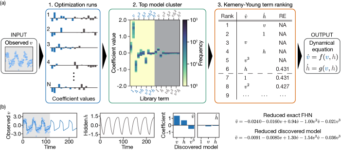
a simplified model of a firing neuron where the membrane voltage $v$ undergoes a rapid increase before being diminished by the slow recovery variable $w$ [45]. The rapid spiking and slow recovery arises from a separation in time scales $\tau\ll 1$ between variables. FHN has become a prototypical model of neuron spike trains, as it is stable and parsimonious, relying only on a small number of polynomial terms. The HDI framework aims to learn models of this type from limited noisy recordings of a single variable, for example the $v$-coordinate of FHN [Fig. 1(a)]. This motivates us to define the following class of models, with observed variables $x_{1},\ldots,x_{m}$ and hidden variables $h_{m+1},\dots,h_{M}$, given by

$$\dot{x}_{k} =\tau_{k}\sum_{|\bm{\alpha}|\leq d_{k}}c_{\bm{\alpha}}^{k}x_{1}^{\alpha_{1}}\ldots h_{M}^{\alpha_{M}},\quad 1\leq k\leq m$$ (2a)

$$\dot{h}_{k} =\tau_{k}\sum_{|\bm{\alpha}|\leq d_{k}}c_{\bm{\alpha}}^{k}x_{1}^{\alpha_{1}}\ldots h_{M}^{\alpha_{M}},\quad m<k\leq M$$ (2b)

which encompass a broad range of nonlinear oscillatory dynamics. Here, we only use polynomial terms on the right-hand side of the equation, although this can be extended to any other nonlinearities, such as trigonometric functions (SI). To avoid scaling ambiguities between $\tau_{k}$ and $\mathbf{c}^{k}=\{c_{\bm{\alpha}}^{k}\}$ in Eq. (2) we enforce that each $\mathbf{c}^{k}$ has unit norm. HDI models are determined by a parameter vector $\mathbf{p}$ containing the initial conditions of the variables $\{x_{k}^{0}\}_{k=1}^{m},\{h_{k}^{0}\}_{k=m+1}^{M}$, time scales $\{\tau_{k}\}_{k=1}^{M}$, and polynomial coefficients $\{\mathbf{c}^{k}\}_{k=1}^{M}$. While time-delay embeddings can be used to provide lower bound estimates on the number of hidden variables $M-m$, here we restrict to periodic models with $M=2$ variables or chaotic models with $M=3$ variables, which we find sufficient to explain the experimental data.

To demonstrate the HDI framework (Fig. 1), we consider noise-corrupted observations $y_{i1}=v(t_{i})+\xi_{i1}$ of the $v$-coordinate of the FHN model (1) [Fig. 1(a, INPUT)]. HDI repeatedly fits hidden two-variable models $(x_{1},h_{1})$ by minimizing the mean square error on the observed variables

$$\text{MSE}(\mathbf{p})=\frac{1}{n}\sum_{i=1}^{n}\sum_{k=1}^{m}(x_{k}(t_{i},\mathbf{p})-y_{ik})^{2}$$ (3)

plus a regularization term $\text{Reg}(\mathbf{p})$ that enforces the unit norm constraint on $\mathbf{c}^{k}$ and promotes sparsity, favoring lower-order terms that often lead to more stable dynamics (SI). The full objective function $L(\mathbf{p})=\text{MSE}(\mathbf{p})+\text{Reg}(\mathbf{p})$ is minimized using ODE sensitivities and gradient descent methods [46, 47] from random initializations [Fig. 1(a, 1)]. Noise robustness in our approach comes from using the full ODE solution $x_{k}(t_{i},\mathbf{p})$ in the objective function, which avoids numerically differentiating noisy time series data, a typically ill-posed problem [48], and enforces that models learned are stable over the time-span of the training data. Multiple fits are required to sufficiently sample multiple local minima of the complex non-convex loss landscape $L(\mathbf{p})$: the model described by $\mathbf{p}$ is not unique since model symmetries – linear, $h\mapsto\alpha h+\beta$, and nonlinear transformations of the hidden variables – produce new models with identical $x_{k}$ dynamics (SI).

To select a single candidate model, a set of models are optimized from random initialization. Model quality is measured using the relative error $\text{RE}(\mathbf{p})=\sqrt{\text{MSE}(\mathbf{p})/\text{Var}(\{y_{i1}\}_{i=1}^{n})}$, given here for a single ($m=1$) observable, where Var is the uncorrected sample variance. Outlier models with incorrect dynamics (nonperiodic, nonchaotic, divergent, etc.) or large RE values are removed in an automated manner, and the remaining models are hierarchically clustered using the cosine similarity between their parameter vectors taking into account possible linear hidden variable transformations (SI). Measurement noise and regularization break many of the symmetry ambiguities resulting in a dominant largest cluster; on FHN data corrupted by $50\%$ noise we start by optimizing $20,000$ dense two-variable cubic models resulting in 4,006 filtered models of which 427 models form the dominant cluster [Fig. 1(a, 2)]. Sparse models are identified from the dominant cluster by ranking each term by its coefficient of variation in the cluster, the interquartile range divided by the median. Rankings are aggregated over a range of clustering thresholds using the Kemeny-Young method to provide a robust ordering of terms. Based on this ordering, a list of candidate models of decreasing sparsity containing the top ranked $s$ terms can be refit [Fig. 1(a, 3)]. From this list, practitioners can determine a suitable model sparsity that balances the trade-off between a model’s complexity and RE based on their scientific judgement [Fig. 1(a, OUTPUT)].

From just three noisy oscillations of the FHN $v$-coordinate, we learn a list of two-variable HDI models that at sparsities six and seven recovers models which are equivalent to FHN [Fig. 1(a, 3)]. The seven-term model matches the sparsity pattern of FHN while the six-term model is equivalent under the shift $w\mapsto w-I$ in Eq. (1). Indeed by taking the true FHN model in Eq. (1), solving for $w$ in terms of $v,\dot{v}$ and substituting into the $\dot{w}$ equation, we obtain a second-order reduced model solely in $v$. Performing a similar reduction of our learned six-term model (SI) we see it has the same structure and similar coefficients as the true FHN model [Fig. 1(b)], confirming that HDI has recovered a two-variable model that is equivalent to ground-truth FHN. We develop an algebraic procedure (SI) to automatically verify these polynomial model reductions on future examples.

At this point, one might hope to avoid using hidden variables and their associated ambiguities by learning the reduced higher-order equation in the observed variable directly [49, 50]. However, even simple multivariate systems can give rise to complex reduced higher-order equations that are often less sparse, implicit and contain fractional powers [51, 52, 53, 54, 55, 56, 57, 58, 59]; for example $\dot{x}=xy^{3},\,\dot{y}=x$ reduces to $x\ddot{x}=\dot{x}^{2}+3x^{7/3}\dot{x}^{2/3}$. Working with reduced-models directly would require learning dense implicit ODEs with more candidate terms [60, 61], a challenging approach which can be ill-posed [62]. A general advantage of ‘first-order’ HDI is that it robustly learns multivariate explicit ODE models that are sparse and integrable, avoiding the above complications. We next apply HDI to identify quantitative models from experimental data for neuron activity and chemical reactions.

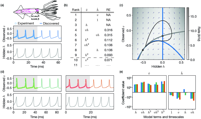
Figure 2(a) shows experimental measurements [42, 43] of the membrane potential $v$ in the giant axon of the North Atlantic longfin inshore squid (Loligo pealeii) in response to noisy stimulus input currents. Following previous spike train model formulations [45, 63, 64, 65], we apply HDI to the time series data for $v$ to learn a sparse two-variable model [Fig. 2(a,b)]. Consistent with prior descriptions of neuron dynamics [15], the phase portrait of the discovered seven-term model is governed by a homoclinic orbit [Fig. 2(c)]. Importantly, the model generalizes to describe recordings from different squids, yielding consistent coefficients across all samples [Fig. 2(d,e)].

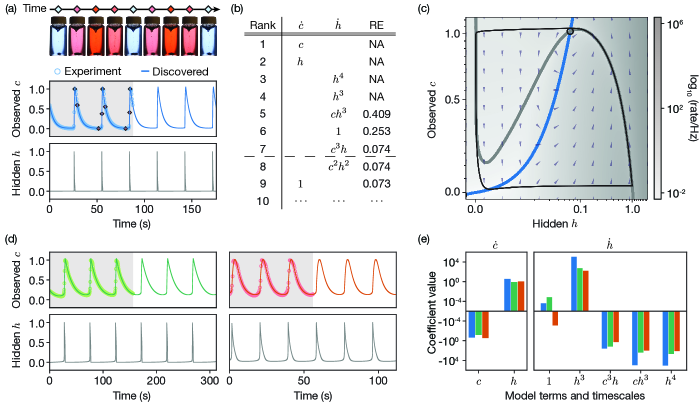
For a second more challenging HDI application, we performed Belousov-Zhabotinsky (BZ) reaction experiments [66]. Over the course of the reaction a substrate species is slowly consumed that fuels the periodic rise and decay of intermediary reagents far from thermodynamic equilibrium. The basic reaction scheme [67] involves more than 20 chemical species and 40 reaction steps. A plethora of different chemical models have been developed that capture the BZ reaction qualitatively [68, 44, 69, 70, 71]. In our experiments, the repeated oxidation and reduction of the metal catalyst ferroin produces a periodic change in color of the solution from red to light blue [Fig. 3(a)]. The recorded average color of the solution follows a 1D curve in color space which we map to our single observed coordinate $c(t)$ (SI). Working with polynomial approximations consistent with established two-variable BZ models [66], we optimize over all two-variable ODEs that are linear in the $\dot{c}$ equation and quartic in the $\dot{h}$ equation. Using this library, HDI discovers a seven-term model that accurately fits the color dynamics $c(t)$ for BZ reactions [Fig. 3(a, d)] with parameters that vary smoothly across the different reactant concentrations in each experiment [Fig. 3(e)]. Furthermore, the phase portrait of the learned model correctly captures the dynamical properties of the BZ reaction [66], showing an unstable fixed point enclosed in a stable limit cycle with a typical cubic-shaped nullcline $\dot{h}=0$ [Fig. 3(c)].

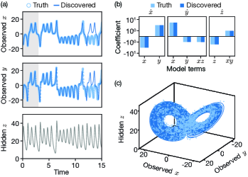
HDI straightforwardly extends to higher-dimensional nonlinear systems. For example, when only given observations of the $x$ and $y$ coordinates of the 3D Lorenz system for one or two lobe transitions [gray-shaded in Fig. 4(a)], a HDI search over all polynomial three-variable ODEs in $(x,y,z)$ with quadratic interactions recovers the exact Lorenz equations with correct coefficient values (modulo a trivial scaling of the hidden $z$ variable) [Fig. 4(b); SI]. The learned model has the correct attractor dynamics and can predict the $x,y,$ and $z$ dynamics substantially beyond the training interval [Fig. 4(a,c)]. Further analysis shows that, even when only given observations of $x$, HDI learns a predictive model for Lorenz dynamics, albeit with reduced predictive power (SI).

Figure 4: HDI discovers true Lorenz system from observations of $x$ and $y$ coordinates. (a) Given observations of only the $x$ and $y$ coordinates (gray region), the learned model predicts the evolution for several additional Lyapunov time-scales. (b) Lorenz model terms and coefficients are discovered exactly by HDI search solely from data in gray region of previous panel. (c) Reconstructed attractor of learned model closely agrees with the true Lorenz attractor (simulation parameters and noise robustness in SI).

To conclude, by combining sensitivity methods and ranked choice voting, HDI can discover parsimonious predictive models from partial noisy observations of oscillatory and chaotic dynamics without extensive preprocessing of time-series data. The above framework can be directly applied to experimental observations of biophysical, ecological and other systems, for which ODE models can inform the prediction, control and optimal perturbations [72] of dynamical behavior. By mapping time series to ODE model coefficients, HDI can help facilitate clustering of dynamical data, as those appearing in health  [73] and climate [8] studies.