LANe : Lighting-Aware Neural Fields for Compositional Scene Synthesis
Abstract
Neural fields††*equal contribution have recently enjoyed great success in representing and rendering 3D scenes. However, most state-of-the-art implicit representations model static or dynamic scenes as a whole, with minor variations. Existing work on learning disentangled world and object neural fields do not consider the problem of composing objects into different world neural fields in a lighting-aware manner. We present Lighting-Aware Neural Field (LANe) for the compositional synthesis of driving scenes in a physically consistent manner. Specifically, we learn a scene representation that disentangles the static background and transient elements into a world-NeRF and class-specific object-NeRFs to allow compositional synthesis of multiple objects in the scene. Furthermore, we explicitly designed both the world and object models to handle lighting variation, which allows us to compose objects into scenes with spatially varying lighting. This is achieved by constructing a light field of the scene and using it in conjunction with a learned shader to modulate the appearance of the object NeRFs. We demonstrate the performance of our model on a synthetic dataset of diverse lighting conditions rendered with the CARLA simulator, as well as a novel real-world dataset of cars collected at different times of the day. Our approach shows that it outperforms state-of-the-art compositional scene synthesis on the challenging dataset setup, via composing object-NeRFs learned from one scene into an entirely different scene whilst still respecting the lighting variations in the novel scene. For more results, please visit our project website https://lane-composition.github.io/.
![[Uncaptioned image]](/html/2304.03280/assets/images/Teaser_lane_lab.png)
1 Introduction
Controllable synthesis of a wide variety of road scenes is of particular interest for training and validating autonomous driving perception systems. Specifically, tasks such as re-simulation and synthesis of rare scenarios require control of a wide variety of 3D scene properties. Precise and controllable 3D scene generation has been a long-standing challenge in computer vision. While there has been significant progress in developing traditional photo-realistic rendering engines [8], they still suffer from the synthetic to real domain gap. Furthermore, significant effort is expended to author photo-realistic 3D assets. This often requires considerable artistic skill and expertise, not to mention cost. In contrast, existing model-based simulators [5, 9] provide controllable synthesis of scenes and images without the need for digital artists. However, they still suffer from a distribution shift with respect to real world images.
Neural Radiance Fields (NeRFs), a state-of-the-art neural rendering technique, offer a promising solution to this problem. NeRFs have been leveraged for learning 3D scene representations for both simple synthetic scenes as well as complex, in-the-wild, multi-view image datasets [21, 41, 26, 35, 43, 10]. However, most NeRF research addresses the problem of modelling a 3D scene as a whole, which does not allow for composition.
As shown in Fig. 1, we investigate the task of inserting cars into driving scenes, where both the scene and the car are represented by 3D neural representations learned from 2D image sequences. Our scene and object representations are lighting aware. This allows us to insert objects in novel poses and novel scenes, while modulating their appearance to be locally consistent with the lighting of the scene.
Our work builds upon recent works that have also addressed the problem of compositional scene modeling with NeRFs by separating scene and object models. Neural Scene Graphs[22] learned a scene graph to model the driving scene, with world and object models represented by implicit representations, but were limited to the same source lighting conditions. Panoptic neural fields[16] includes representations like semantic and instance segmentation allowing for more fine grained addition and removal of objects in the scene. Several other works such as [37, 38], representing dynamic scenes present frameworks to separate the static and dynamic components. Most of these frameworks ground the dynamic component either to a time variable or to a learnt latent variable. This assumption restricts the variation in object compositions that can be performed with respect to scene. However, in all such previous works, the composition is not lighting-aware (i.e the object’s appearance is inconsistent with the scene’s lighting conditions).
The limitations of prior work [22, 16, 37, 38] fail to produce realistic results by lacking lighting-aware composability. We directly address these shortcomings with our novel approach for scene modeling and object insertion in a lighting-aware manner, without explicitly modelling the materials of the objects and the scenes. To summarize, the contributions of our work are as follows,
-
1.
We present a 3D neural scene representation that represents the scene with a world-NeRF for the background and class-specific object-NeRFs for the dynamic elements, both of which are lighting dependent.
-
2.
We propose a novel approach to modulate the color of the rendered objects in unseen poses and scenes, by augmenting the scene with a spatially varying light field and the object with a lighting-dependent shader.
2 Related Works
2.1 2D methods
2D approaches address the problem of compositional synthesis by alpha compositing different elements of the scene in a layered manner. Omnimatte[19] separates static and dynamic elements of a video and associates correlated dynamic effects to the corresponding element. Layered neural rendering separates out the scene and dynamic elements. Alhaija et al.[1] uses digital assets rendered onto a scene followed by a network to harmonize the inserted object using an adversarial loss. Whilst all these approaches demonstrate the state-of-the-art performance on scene synthesis and composition, they lack 3D scene understanding and the level of controllability of scene manipulation. With 3D geometry and lighting awareness, our approach models both the dynamic and static elements of the scene as implicit representations, allowing for controllable composition of elements into arbitrary locations.
2.2 Explicit 3D methods
Several approaches [25, 45, 11] have since used explicit 3D models for compositional scene synthesis. Specifically, Raj et al.[25] use a mesh proxy to represent the dynamic human avatar and compose it into arbitrary scene using deferred neural rendering. Neural light field for object composition demonstrate it with explicit mesh while estimating lighting of real scenes. From a single 2D image, SIMBAR [45] models the scene as a 3D mesh to explicitly represent scene geometry, followed with shadow refinement network to produce realistic shadows. Granskog et al [11] propose a technique to compose neural scene representation for shading inference, which explicitly distentangles lighting, material, and geometric information using illumination buffers. These discussed explicit 3D methods lack object-aware composition capability with the scene.
2.3 Implicit 3D methods
Several recent methods study the problem of composing scene elements with implicit representation[21, 31, 41, 40, 39, 24], which have gained a great success in modeling scenes. Particularly, ObjectNeRF [37] consists of an object model that is used to represents parts of the scene other than the background, and a scene model that is responsible for recomposing the decomposed objects to the scene. Neural Scene Graphs (NSG) [22] models driving scenes with a world model and object models of learned scene graph representation, which encodes object transformation and radiance. Panoptic Neural Fields [15] extends NSG to predicts panoptic-radiance field that encodes color, density and semantic segmentation labels of the objects in the scene. However, most of the models do not model effect of lighting changes on the scene or objects.
2.4 Lighting-aware representations
Several approaches [3, 33, 44, 4] have worked on lighting-aware manipulation for single objects or scenes. Particularly, NeRF-OSR[28] leveraged scene geometry surface property modeling to account for outdoor scenes captured under varying illumination, but it was restricted mostly to static building architecture. NeRFactor[44] modeled the lighting effect on objects using a BRDF represented by an implicit representation. Zhang et al. [42] proposed to learn object surfaces and use the Phong shading model [23] to capture lighting variations. However, none of these methods address the interactions of objects with their surrounding world, namely, for NeRD, it assumes light sources are at infinity and needs observations of the object at a certain location to build an environment map, or an environment map of the scene at the particular pose that needs to be rendered. Such an approach has the limitation that it is computationally intensive to compute environment maps at each pose.
For compositional synthesis, prior models have not considered whether incident lighting is dependent on the target location for composition within the overall world model. This is an important question is not addressed by work before LANe. Our work is similar in spirit to OSF[12], which is also evaluated primarily on synthetic scenes; however, we note that OSF only primarily works on point light sources in indoor scenes under known lighting conditions. In contrast, our method uses lighting information gathered directly from the scene, and tackles the much harder problem of outdoor scenes. Furthermore, in contrast to methods that model the material properties explicitly, our approach learns the lighting effect as a multiplicative term on top of the learnt radiance without the need to model accurate BRDF material properties. Furthermore, our approach eschews the expensive requirements to compute a lighting representation at each rendered pose, and can interpolate between training poses.
Generating data using continuous composition with spatially varying lighting in outdoor driving scenes, it allows us to facilitate the data need of autonomous driving perception systems. This is the main differentiator between our approach and the existing methods. LANe is able to compose dynamic moving objects(vehicles) and continuously changing outdoor environments in a lighting-aware manner.
3 Approach


3.1 Preliminaries
We base our representations on NeRFs[21, 2], which use MLPs to learn a 3D volumetric model from posed images. Specifically, given a set of images with known camera locations , we learn a scene representation such that pixel value observed along a particular direction is obtained by casting a ray and performing volumetric integration along the ray as follows:
| (1) |
where are the outgoing radiance and density at a 3D point modelled by the NeRF , are the near and far plane boundaries along the ray, and is the accumulated transmittance along the ray, given by
In practice, the discrete version of the integration is performed by quadrature approximation during volume rendering as given by [20].
3.2 Overview
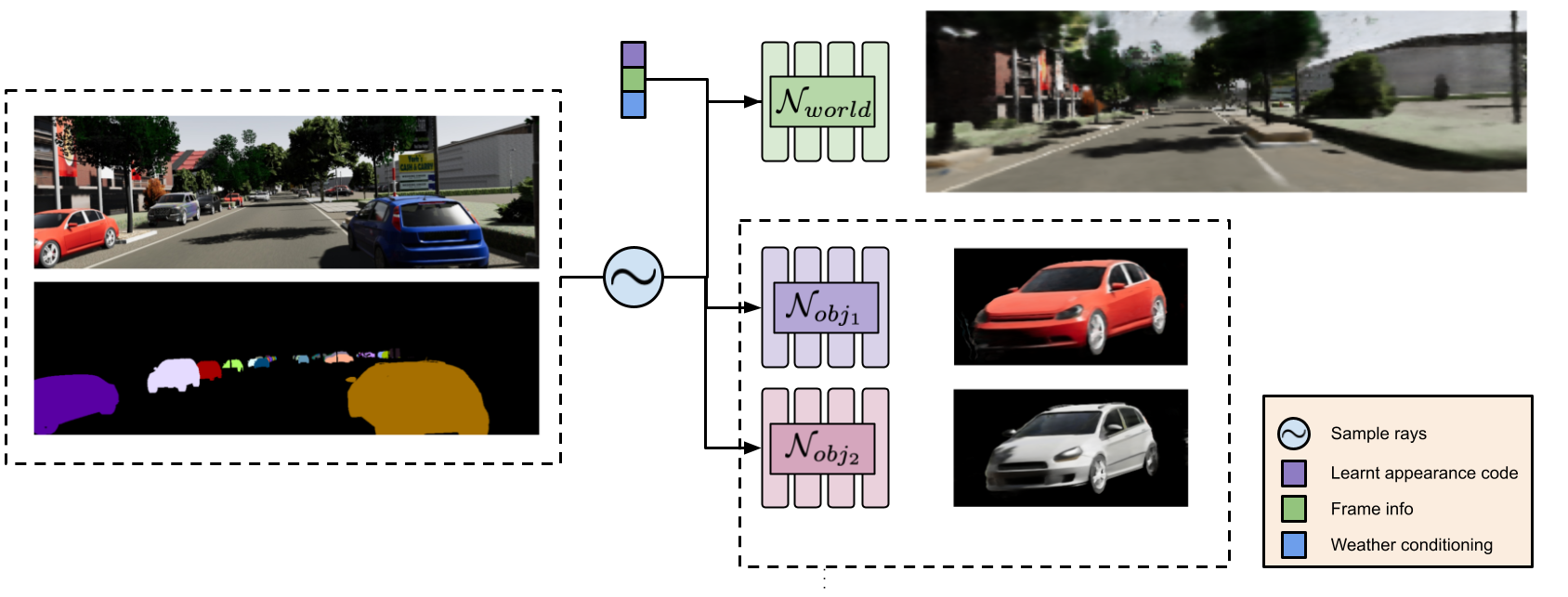
Following [22, 15], as illustrated in Fig. 2, we decompose the scene into a world-NeRF (Sec. 3.3) and an object-NeRF (Sec. 3.4) to represent the static and dynamic components respectively. Additionally, we train both our object and world models in a lighting aware manner, under multiple lighting conditions, to disentangle geometry and albedo from lighting effects. Particularly, our datasets comprise a set of images of multiple scenes under lighting conditions .
For world-NeRFs in driving scenes, we assume a single light source at infinity and model the lighting effects on the world as a function of azimuth and elevation angle . As indicated in Fig. 3, the scene model produces spatially-varying intermediate lighting features that are fed to the object-NeRF to condition the object’s appearance on spatially-varying lighting cues.
3.3 World-NeRF
The scene is modeled by a lighting agnostic network and lighting aware Neural Light field [32]. Particularly,
| (2) |
| (3) |
where is a sample along the ray, and are ray origins and directions, and is a latent feature that parameterizes the scene lighting. This could either be learned or set from physical lighting parameters (sun azimuth and elevation).
Since only takes the spatial position as input but is trained across different lighting conditions, it essentially learns an average color across all lighting variations. The final color of the world scene given by a multiplicative effect of the lighting agnostic scene geometry and the lighting aware scene model. Particularly, we use , the light-field latent, to learn a lighting-specific multiplier.
| (4) |
Where represents a shader function that learns a multiplicative factor to obtain the lighting specific scene radiance from the lighting agnostic color. The light field outputs are also used to shade the inserted object models are described in 3.4.
3.4 Object-NeRF
The object model, similar to the world model, has two components: a scene-agnostic representation for density and color (albedo) , and a scene-dependent shader for radiance . The coordinate inputs to the models and are represented in normalized object coordinate frames[36]. Their weights are shared across object instances of the same semantic class (cars) with different colors and shapes, by using instance-specific shape and color codes inspired by [14, 18].
Specifically, the scene-agnostic representation is modeled as:
| (5) |
above is the lighting-agnostic radiance of the object. The lighting conditioned radiance is obtained by multiplying with a shading coefficient predicted by .
| (6) |
We then use during volumetric rendering as in [21]. is the position encoding applied to its inputs, as is standard practice for neural fields. We explore different shader architectures optimized for two different downstream applications: for composing objects into new locations within the same scene, and for composing into new scenes. These reflect two methods for feeding information from the world representation to the object shading representation.
3.4.1 Composing into known scenes
For composing an object model into new locations in scenes where it has already been observed, the input coordinates has been fed in the global frame in addition to the coordinates in object coordinate information to represent a lighting aware object model. Specifically, given the 3D bounding box of the car with parameters and , we transform the rays cast into the scene into object coordinate system as follows.
| (7) |
Then the shading network is modelled as:
| (8) |
where is a learnable scene specification that allows us to share weights for between scenes. The shading network learns to shade the point at differently based on its global state ().
3.4.2 Composing into unknown scenes
To insert our object model into scenes where the object has not been observed during training, we need a shading model that does not specifically memorize the scene. To this end, we learn a generalizable shader that uses the light-field of the target scene to compute Recollect that the rendering equation for the output radiance at a point can be written as follows:
| (9) |
Where, and are incoming and outgoing ray directions respectively, is the normal calculated at the surface and is the viewing direction. Here, we model with the scene light-field . We also assume a Lambertian model of the object, which reduces to a constant. We approximate the integral by a weighted sum. In particular, for each point on the surface of the object to be rendered , we cast secondary rays to evaluate the incoming light as
| (10) |
Since the normals from the density fields can be noisy, we use attention layers, with the local car coordinates as queries, and the incident lighting values along with directions as keys and values, to summarize the incident lighting at each point in a feature . More details about the attention mechanism are provided in supplementary.
This accumulated feature is fed into a shading MLP along with the coordinates of the point in the local car coordinates to predict a shading value.
| (11) |
3.5 Training
We train the object-NeRF and world-NeRF with the following objectives:
Photo-metric loss: This encourages the rendered pixel to match the color of the ground truth pixel color .
| (12) |
Mask-loss : We find that the mask loss is necessary to separate out the objects from the scene.
| (13) |
where and represents the accumulated alpha value along a ray and ground truth mask respectively.
Depth guidance : In datasets where we have access to depth/lidar information, we leverage depth for the training rays in the world-NeRF as in [6, 27].
| (14) |
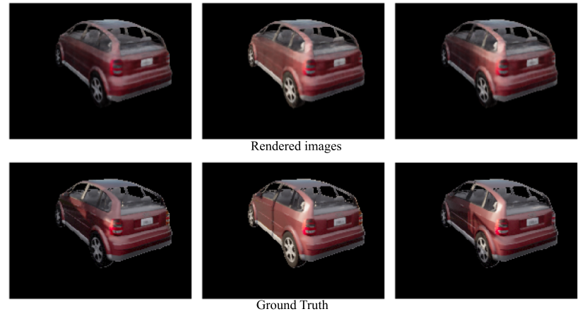
Furthermore, we find that, coarse to fine grained optimization helps in improving the quality of the learnt object model.
The loss for the world model is then given as follows:
| (15) |
And the corresponding object model is given by:
| (16) |
The lighting-agnostic object and world models can be trained independently as we have annotations for the static and dynamic components of the scene. The training of the object model uses the light field component of the world model.
4 Experiments
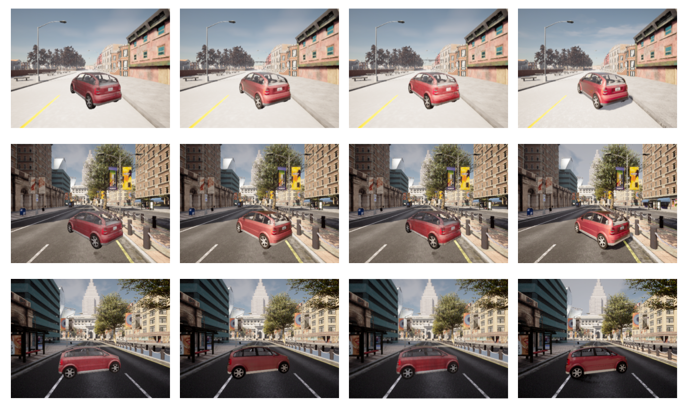
Our experiments evaluate the quality of images rendered when composing LANe models into unseen poses (Fig. 3) within both seen and unseen worlds. For seen environments, we report metrics for both the local-global coordinate shader (Sec. 3.4.1) as well as the light-field conditioned shader (Sec. 3.4.2), although the main benefit of the latter is its ability to generalize to unseen environments.
4.1 Architecture details
World NeRFs Our world NeRF is represented as a standard NeRF with 8 MLP layers and a parallel branch with 4 MLP layers to control the lighting of the associated scene. We use a similar 8-layer MLP to learn a light field network for the scene.
Object NeRFs Our base object NeRF follows a similar 8-layer MLP architecture.
Object Shader In known scenes, the shader network is simply another MLP that accepts the global coordinates and the orientation of the car as a quaternion. The shader network for unknown scenes is modeled as an attention-conditioned MLP with the local coordinate attending over sampled light field directions and values.
4.2 Datasets
Synthetic CARLA dataset We use the CARLA simulator [7] to render images of multiple urban scenes under varying lighting conditions with vehicles in different poses in the scene. We render 8 scenes under different lighting conditions with 5 different car instances observed in 40 different locations in each scene. We divide the scenes into 6 training scenes and 2 test scenes for evaluating composition into novel scenes. Within each scene, we also hold-out 20% of the locations, to evaluate composition in known scenes. Unlike many other NeRF datasets, our camera orientation does not vary significantly, to be representative of real-world car data.
Real world dataset To evaluate the applicability of our approach to real world images, we collect a real world multi-view dataset of 4 different cars at 10 different times of the day. Each instance comprises videos from a handheld mobile camera revolved around the car. 100 frames are extracted from each video to train object and world models. We estimate the camera poses using COLMAP [29, 30], predict 2D instance segmentation masks using an off-the-shelf model [13], and manually label approximate 3D bounding boxes from COLMAP reconstruction.
| Scene 1 | Scene 2 | Scene 3 | |||||||
|---|---|---|---|---|---|---|---|---|---|
| SSIM | PSNR | LPIPS | SSIM | PSNR | LPIPS | SSIM | PSNR | LPIPS | |
| NeRF | |||||||||
| LANe (Single) | |||||||||
| LANe (Multiple) | |||||||||
| LANe (LF) | |||||||||
4.3 Baselines
NeRF We compare our method against lighting agnostic compositional 3D scene synthesis methods [22, 15] by using a vanilla NeRF model as the object representation. Although they are not directly applicable to composable representations of dynamic objects, we explore the use of relightable NeRF methods [3] in the supplementary material.
4.4 Known worlds lighting-aware composition
In this experiment (shown in Fig. 4), we evaluate the quality of composing LANe object models into unseen poses in 3 environments with both globally as well as locally varying lighting conditions. These world environments have been used during training. Our results are reported in Tab. 1. We find that when composing into environments seen during training, the local-global architecture greatly outperforms other approaches.
4.5 Unseen worlds lighting-aware composition
Only the light-field conditioned shading architecture (LANe-LF) is suitable for composition into unseen world models. In Fig. 5, we compare this against the vanilla NeRF model and the local-global architecture (both of which have used this environment during training) in Table 3. We find that while LANe-LF is clearly better than a lighting-agnostic NeRF model, it is still slightly worse, but comparable in quality to a local-global model which was trained on this world.
4.6 Real-world lighting aware composition
| Method | SSIM | PSNR | LPIPS |
|---|---|---|---|
| NeRF only | 24.390 | ||
| LANe (LF) | 26.637 |
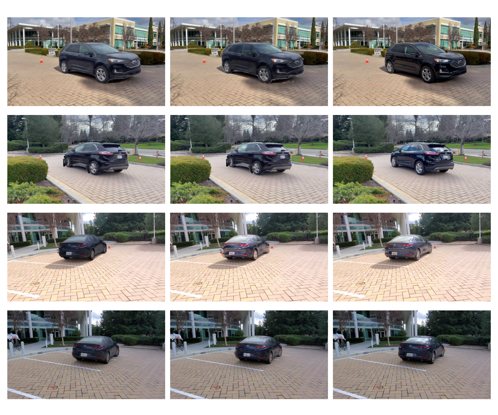
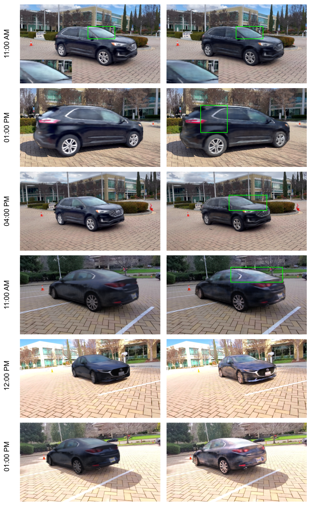
For real scenes, the lighting aware object models are trained along with the world light fields, and composed into seen and unseen scenes. The results are as shown in Fig. 6. Note that the unshaded lighting-agnostic object models still have some lighting artifacts in regions that were well-lit. The shader compensates for this, and brightens specular and well-lit regions on the car, while darkening regions that are not well-lit. The quantitative evaluation on the composition of the lighting-aware object model on held-out views and report findings are listed in Tab. 2. The metrics show that the model shades the object in a lighting-consistent manner even in such scenes with challenging lighting and reflections.
We find that training the attention-based shader architecture from Sec. 3.4.2 is challenging when objects are observed in only 7 lighting conditions. We therefore use global lighting features with the object shader, which captures inter-scene lighting information, but limits the spatial variance of object’s appearance within the scene.
4.7 Ablations
Local-Global NeRFs for a single vs multiple objects From Tab. 1, we observe training instance-specific lighting-aware models performs better than a shared model conditioned on an instance-specific latent code. Using a latent space to model multiple instances can however still be useful in practical settings where a single instance may not be observed in several parts of the scene. The multi-instance model would be able to share lighting information across instances.
4.7.1 Local-Global Net architecture
Our proposed local-global net architecture uses the local coordinates for the density branch and the global coordinates for the radiance branch. We find that this separation of global and local coordinates is crucial, and that merely using the global coordinates as an input to the density branch along with the local coordinates results in the network learning incorrect densities, especially without a mask loss.
We train a model with a global conditioning code instead of spatially varying local code as explained in our model.
| FID | SSIM | PSNR | LPIPS | |
|---|---|---|---|---|
| NeRF only | ||||
| LANe (multiple) | ||||
| LANe (LF) |
5 Discussions
The dataset generated by CARLA exhibit spatially varying lighting effects due to both direct (sun) and indirect lighting (shadows cast by buildings). We see from Table. 1 that our model is able to better capture changes in object lighting as it moves through the scene. Particularly, we see that a naive conditional baseline is insufficient as it correlates scene effects and object effects. Further more, naive conditioning requires large amount of data to accurate model the light transport across the scene.
Kundu et al. [15] model each object with a seperate light MLP. using FedAvg to build in class priors. However, these model grows linearly in the number of objects being represented. We employ a variant of CodeNerf [14] to allow for larger degree of control over the class of objects without explosion in memory bandwidth.
6 Limitations and Conclusion
Limitation and future work Our framework assumes observations of the object under varying lighting which limits its applicability to the scenes where an object is seen under varying lighting conditions. This can be addressed using shading methods trained on both synthetic and real data. In addition,our approach does not model object-to-scene and object-to-object shadows. The shadows in real results are residuals from background. Addressing this would involves re-evaluating the lighting on an object once another is added, and is an exciting problem for future work, potentially using shadow fields for each instance that are dependent on the same lighting representation. Our model, much like many of the cited works, is sensitive to the pose parameters and object masks and pose robustness is outside the scope of our approach. However, recent works which are robust to camera pose (such as BARF [17] or SPARF[34]) can potentially be leveraged to address this problem.
Conclusion In this work, we introduce an approach to leverage spatial lighting-aware NeRFs to build composable 3D scene representations. We separate the scene into object and world NeRFs and introduce a multiplicative shading model to condition the object’s appearance on the scene lighting. This allows our object models to be composed into new world models in a lighting-aware manner without retraining any object parameters.
References
- [1] Hassan Abu Alhaija, Siva Karthik Mustikovela, Andreas Geiger, and Carsten Rother. Geometric image synthesis. arXiv preprint arXiv:1809.04696, 2018.
- [2] Jonathan T Barron, Ben Mildenhall, Matthew Tancik, Peter Hedman, Ricardo Martin-Brualla, and Pratul P Srinivasan. Mip-NeRF: A multiscale representation for anti-aliasing neural radiance fields. ICCV, 2021.
- [3] Mark Boss, Raphael Braun, Varun Jampani, Jonathan T Barron, Ce Liu, and Hendrik Lensch. Nerd: Neural reflectance decomposition from image collections. In Proceedings of the IEEE/CVF International Conference on Computer Vision, pages 12684–12694, 2021.
- [4] Mark Boss, Varun Jampani, Raphael Braun, Ce Liu, Jonathan Barron, and Hendrik Lensch. Neural-pil: Neural pre-integrated lighting for reflectance decomposition. Advances in Neural Information Processing Systems, 34:10691–10704, 2021.
- [5] Yohann Cabon, Naila Murray, and Martin Humenberger. Virtual kitti 2. arXiv preprint arXiv:2001.10773, 2020.
- [6] Kangle Deng, Andrew Liu, Jun-Yan Zhu, and Deva Ramanan. Depth-supervised nerf: Fewer views and faster training for free. In Proceedings of the IEEE/CVF Conference on Computer Vision and Pattern Recognition, pages 12882–12891, 2022.
- [7] Alexey Dosovitskiy, German Ros, Felipe Codevilla, Antonio Lopez, and Vladlen Koltun. Carla: An open urban driving simulator. In Conference on robot learning, pages 1–16. PMLR, 2017.
- [8] Alexey Dosovitskiy, Germán Ros, Felipe Codevilla, Antonio M. López, and Vladlen Koltun. CARLA: an open urban driving simulator. CoRR, abs/1711.03938, 2017.
- [9] Adrien Gaidon, Qiao Wang, Yohann Cabon, and Eleonora Vig. Virtual worlds as proxy for multi-object tracking analysis. In Proceedings of the IEEE conference on Computer Vision and Pattern Recognition, pages 4340–4349, 2016.
- [10] Chen Gao, Ayush Saraf, Johannes Kopf, and Jia-Bin Huang. Dynamic view synthesis from dynamic monocular video. In Proceedings of the IEEE/CVF International Conference on Computer Vision, pages 5712–5721, 2021.
- [11] Jonathan Granskog, Fabrice Rousselle, Marios Papas, and Jan Novák. Compositional neural scene representations for shading inference. ACM Trans. Graph., 39(4), aug 2020.
- [12] Michelle Guo, Alireza Fathi, Jiajun Wu, and Thomas A. Funkhouser. Object-centric neural scene rendering. CoRR, abs/2012.08503, 2020.
- [13] Kaiming He, Georgia Gkioxari, Piotr Dollár, and Ross Girshick. Mask r-cnn. In 2017 IEEE International Conference on Computer Vision (ICCV), pages 2980–2988, 2017.
- [14] Wonbong Jang and Lourdes Agapito. Codenerf: Disentangled neural radiance fields for object categories. In Proceedings of the IEEE/CVF International Conference on Computer Vision, pages 12949–12958, 2021.
- [15] Abhijit Kundu, Kyle Genova, Xiaoqi Yin, Alireza Fathi, Caroline Pantofaru, Leonidas J Guibas, Andrea Tagliasacchi, Frank Dellaert, and Thomas Funkhouser. Panoptic neural fields: A semantic object-aware neural scene representation. In Proceedings of the IEEE/CVF Conference on Computer Vision and Pattern Recognition, pages 12871–12881, 2022.
- [16] Jogendra Nath Kundu, Mugalodi Rakesh, Varun Jampani, Rahul Mysore Venkatesh, and R Venkatesh Babu. Appearance consensus driven self-supervised human mesh recovery. In ECCV, 2020.
- [17] Chen-Hsuan Lin, Wei-Chiu Ma, Antonio Torralba, and Simon Lucey. BARF: bundle-adjusting neural radiance fields. CoRR, abs/2104.06405, 2021.
- [18] Steven Liu, Xiuming Zhang, Zhoutong Zhang, Richard Zhang, Jun-Yan Zhu, and Bryan Russell. Editing conditional radiance fields. In Proceedings of the IEEE/CVF International Conference on Computer Vision, pages 5773–5783, 2021.
- [19] Erika Lu, Forrester Cole, Tali Dekel, Andrew Zisserman, William T Freeman, and Michael Rubinstein. Omnimatte: Associating objects and their effects in video. In Proceedings of the IEEE/CVF Conference on Computer Vision and Pattern Recognition, pages 4507–4515, 2021.
- [20] Nelson Max. Optical models for direct volume rendering. IEEE Transactions on Visualization and Computer Graphics, 1(2):99–108, 1995.
- [21] Ben Mildenhall, Pratul P. Srinivasan, Matthew Tancik, Jonathan T. Barron, Ravi Ramamoorthi, and Ren Ng. NeRF: Representing scenes as neural radiance fields for view synthesis. In ECCV, 2020.
- [22] Julian Ost, Fahim Mannan, Nils Thuerey, Julian Knodt, and Felix Heide. Neural scene graphs for dynamic scenes. In Proceedings of the IEEE/CVF Conference on Computer Vision and Pattern Recognition, pages 2856–2865, 2021.
- [23] Bui Tuong Phong. Illumination for computer generated pictures. Commun. ACM, 18(6):311–317, 1975.
- [24] Amit Raj, Umar Iqbal, Koki Nagano, Sameh Khamis, Pavlo Molchanov, James Hays, and Jan Kautz. Dracon–differentiable rasterization conditioned neural radiance fields for articulated avatars. arXiv preprint arXiv:2203.15798, 2022.
- [25] Amit Raj, Julian Tanke, James Hays, Minh Vo, Carsten Stoll, and Christoph Lassner. Anr-articulated neural rendering for virtual avatars. In IEEE Conf. Comput. Vis. Pattern Recog., 2021.
- [26] Amit Raj, Michael Zollhoefer, Tomas Simon, Jason Saragih, Shunsuke Saito, James Hays, and Stephen Lombardi. Pva: Pixel-aligned volumetric avatars. In IEEE Conf. Comput. Vis. Pattern Recog., 2020.
- [27] Konstantinos Rematas, Andrew Liu, Pratul P Srinivasan, Jonathan T Barron, Andrea Tagliasacchi, Thomas Funkhouser, and Vittorio Ferrari. Urban radiance fields. In Proceedings of the IEEE/CVF Conference on Computer Vision and Pattern Recognition, pages 12932–12942, 2022.
- [28] Viktor Rudnev, Mohamed Elgharib, William Smith, Lingjie Liu, Vladislav Golyanik, and Christian Theobalt. Nerf for outdoor scene relighting. In European Conference on Computer Vision, pages 615–631. Springer, 2022.
- [29] Johannes Lutz Schönberger and Jan-Michael Frahm. Structure-from-motion revisited. In Conference on Computer Vision and Pattern Recognition (CVPR), 2016.
- [30] Johannes L Schonberger and Jan-Michael Frahm. Structure-from-motion revisited. In Proceedings of the IEEE Conference on Computer Vision and Pattern Recognition, pages 4104–4113, 2016.
- [31] Vincent Sitzmann, Julien Martel, Alexander Bergman, David Lindell, and Gordon Wetzstein. Implicit neural representations with periodic activation functions. Advances in Neural Information Processing Systems, 33:7462–7473, 2020.
- [32] Vincent Sitzmann, Semon Rezchikov, Bill Freeman, Josh Tenenbaum, and Fredo Durand. Light field networks: Neural scene representations with single-evaluation rendering. Advances in Neural Information Processing Systems, 34:19313–19325, 2021.
- [33] Pratul P Srinivasan, Boyang Deng, Xiuming Zhang, Matthew Tancik, Ben Mildenhall, and Jonathan T Barron. Nerv: Neural reflectance and visibility fields for relighting and view synthesis. In Proceedings of the IEEE/CVF Conference on Computer Vision and Pattern Recognition, pages 7495–7504, 2021.
- [34] Prune Truong, Marie-Julie Rakotosaona, Fabian Manhardt, and Federico Tombari. Sparf: Neural radiance fields from sparse and noisy poses, 2022.
- [35] Dor Verbin, Peter Hedman, Ben Mildenhall, Todd Zickler, Jonathan T Barron, and Pratul P Srinivasan. Ref-nerf: Structured view-dependent appearance for neural radiance fields. In 2022 IEEE/CVF Conference on Computer Vision and Pattern Recognition (CVPR), pages 5481–5490. IEEE, 2022.
- [36] He Wang, Srinath Sridhar, Jingwei Huang, Julien Valentin, Shuran Song, and Leonidas J Guibas. Normalized object coordinate space for category-level 6d object pose and size estimation. arXiv preprint arXiv:1901.02970, 2019.
- [37] Qianyi Wu, Xian Liu, Yuedong Chen, Kejie Li, Chuanxia Zheng, Jianfei Cai, and Jianmin Zheng. Object-compositional neural implicit surfaces. In European Conference on Computer Vision, pages 197–213. Springer, 2022.
- [38] Tianhao Wu, Fangcheng Zhong, Andrea Tagliasacchi, Forrester Cole, and Cengiz Oztireli. D2nerf: Self-supervised decoupling of dynamic and static objects from a monocular video. arXiv preprint arXiv:2205.15838, 2022.
- [39] Alex Yu, Sara Fridovich-Keil, Matthew Tancik, Qinhong Chen, Benjamin Recht, and Angjoo Kanazawa. Plenoxels: Radiance fields without neural networks. arXiv preprint arXiv:2112.05131, 2021.
- [40] Alex Yu, Ruilong Li, Matthew Tancik, Hao Li, Ren Ng, and Angjoo Kanazawa. Plenoctrees for real-time rendering of neural radiance fields. ICCV, 2021.
- [41] Ning Yu, Vladislav Skripniuk, Sahar Abdelnabi, and Mario Fritz. Artificial fingerprinting for generative models: Rooting deepfake attribution in training data. In ICCV, 2021.
- [42] Jason Zhang, Gengshan Yang, Shubham Tulsiani, and Deva Ramanan. Ners: Neural reflectance surfaces for sparse-view 3d reconstruction in the wild. Advances in Neural Information Processing Systems, 34:29835–29847, 2021.
- [43] Kai Zhang, Gernot Riegler, Noah Snavely, and Vladlen Koltun. Nerf++: Analyzing and improving neural radiance fields. arXiv preprint arXiv:2010.07492, 2020.
- [44] Xiuming Zhang, Pratul P Srinivasan, Boyang Deng, Paul Debevec, William T Freeman, and Jonathan T Barron. Nerfactor: Neural factorization of shape and reflectance under an unknown illumination. ACM Transactions on Graphics (TOG), 40(6):1–18, 2021.
- [45] Xianling Zhang, Nathan Tseng, Ameerah Syed, Rohan Bhasin, and Nikita Jaipuria. SIMBAR: single image-based scene relighting for effective data augmentation for automated driving vision tasks. In IEEE/CVF Conference on Computer Vision and Pattern Recognition, CVPR 2022, New Orleans, LA, USA, June 18-24, 2022, pages 3708–3718. IEEE, 2022.
LANe - Lighting Aware Neural Fields for Compositional Scene Synthesis - Supplementary
Appendix A Introduction
For demo videos of 3D neural rendering and details about the ablation studies, please visit our project website: https://lane-composition.github.io. We also intend to release code and datasets there.
Appendix B Architecture details
The architectures for our world NeRF, world light field network, and object NeRFs are standard MLPs, optionally conditioned on latent codes to share models across instances, and are described in Sections 3.3, 3.4 and 4.1. Here we provide more details on our novel LFN-based shader network presented in Section 3.4.2.
B.1 Unknown scene - LFN based shader field
Lighting-aware composition of neural fields in unknown scenes uses 3 components:
-
1.
Object model: A lighting-agnostic object (car) model that was trained on images from different scenes.
-
2.
Light field network for the scene to be composed into.
-
3.
Shader network for the object to the composed.
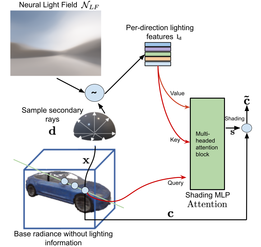
These components are illustrated in (Fig. 7). In particular, the object model
| (17) |
where, are the positional encoding and is the object code for the particular instance of the car model. For composing the objecting into scenes unseen during training, we use the light field of the new scene:
| (18) |
where is the 3D location of a point on the object and is the direction of secondary ray, both expressed in world coordinates, and is the incoming 3-channel LDR radiance at along .
To obtain the shading at a surface point in object coordinate frame, we first compute a local accumulated lighting feature using an attention mechanism:
| (19) |
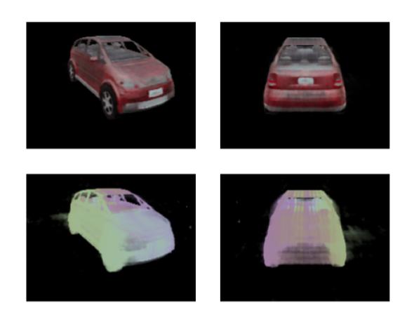
where are queries, keys and values, and are their learnable linear mappings respectively. We use , and , where is the concatenation operator and is the positional encoding. The attention mechanism has been leveraged to encourage the network to focus on some of all incoming light, conditioning on its local coordinates. This resembles the weighted integral of irradiance based on the incident angle in the rendering equation. Ideally, we expect the attention weights to be higher along the direction of the surface normal at the point. We visualize the attended direction at each surface point by obtaining the weighted average secondary direction using the learned attention weights (the “attended direction”) in Fig. 8. This shows that the attended direction aligns with the surface normals on the surface of a single car instance.
We then use a 4-layer MLP to predict a 3-channel shading coefficient for each point on the object conditioned on the learned accumulated lighting feature:
| (20) |
where is the latent code for the specific instance. Note that we only train on points on the surface the object by thresholding points with an occupancy value greater than 0.5, to avoid sampling secondary rays at all points.
Appendix C Dataset details
In this section we describe and provide examples from the synthetic and real datasets used to train our models.
C.1 Synthetic dataset
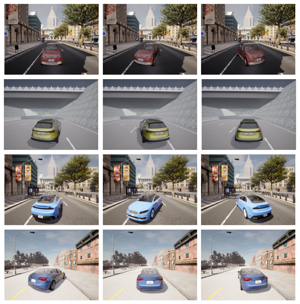
Our synthetic dataset comprises 6 different car instances rendered in 10 different lighting conditions using the CARLA simulator. Each lighting condition can be in one of 5 different scenes. Within each lighting condition, the car is observed in multiple positions within the scene, at different orientations. The camera viewpoint does not change significantly, but we still obtain images of different portions of the car as the car still has different poses with respect to the scene. This resembles the conditions encountered in real world self-driving datasets. We also use 3D bounding boxes and instance masks from the simulator. Examples from our dataset is illustrated in Fig 9.
C.2 Real dataset
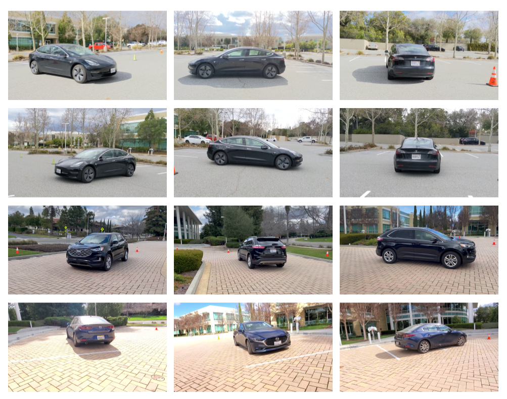
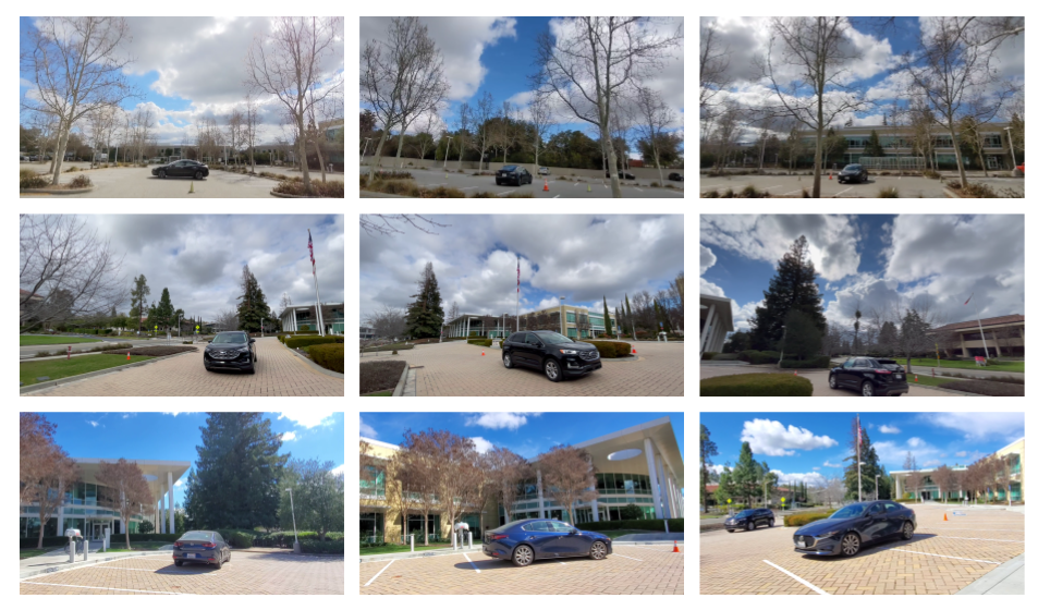
Our real dataset features sequences of images collected by moving a handheld camera around a parked vehicle. We collect sequences for the same vehicle at 10 different times of the day, for 3 different vehicles. Each vehicle is parked in a slightly different scene. At each time of day, we also collect an additional sequence with the camera zoomed out, so as to capture sky lighting and train a light field model with it. We use 100 images from each sequence for training the object and shader models, and 50 images for training the world light field models. We register all images for a particular instance into a common frame of reference using COLMAP [29]. The local frame for the vehicle is defined by manually annotating a 3D bounding box around the instance from the sparse COLMAP reconstruction. Instance masks are obtained from a pretrained Mask R-CNN [13] model. Examples from the object model sequences are shown in Fig 10 and the light-field model sequences are shown in 11.
Appendix D More qualitative results
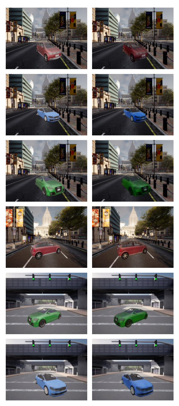
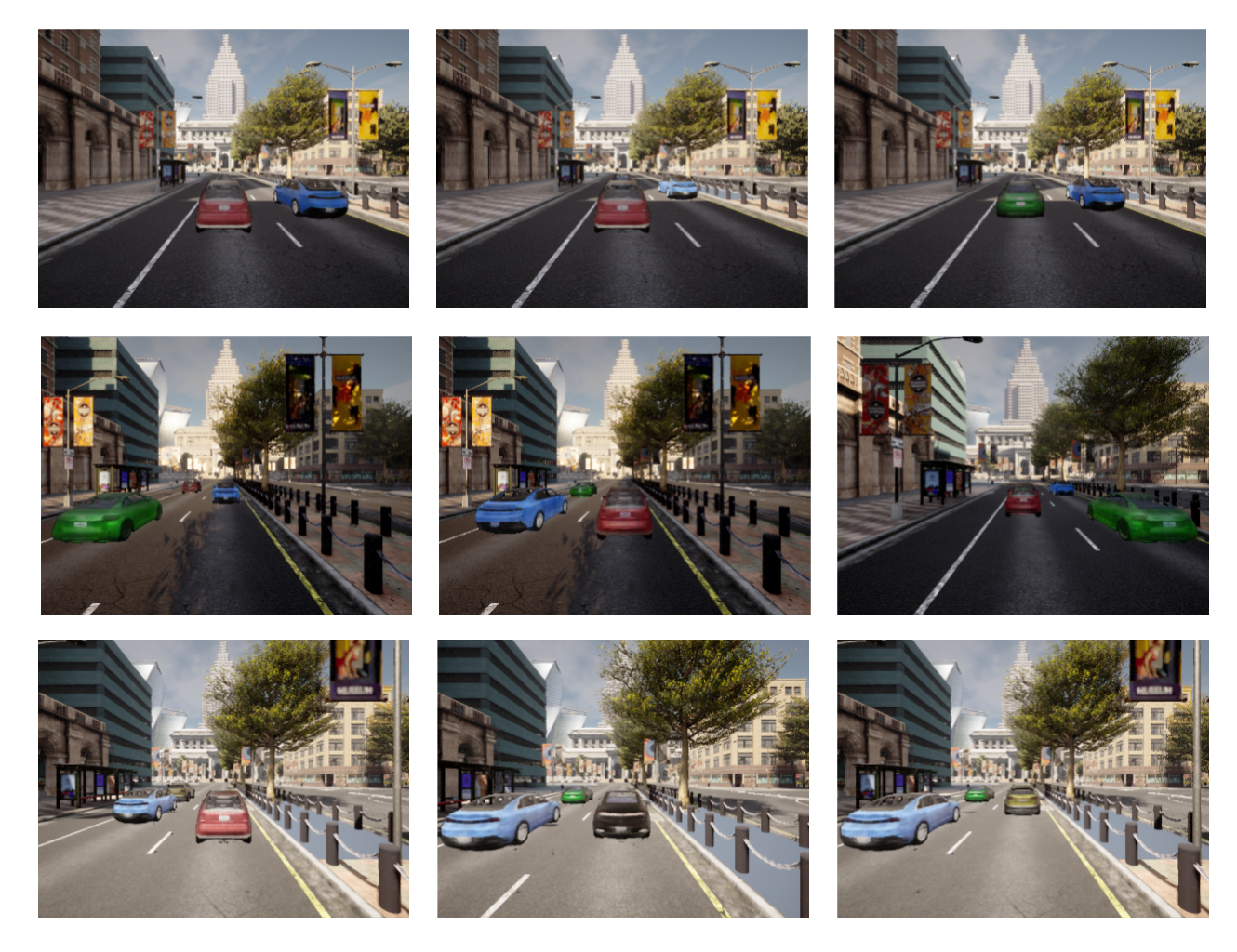
More qualitative results are provided for composing lighting-aware object models into both known and unknown scenes, for both synthetic (Fig 12, 15) and real datasets (Fig 13). Our approach also allows us to compose multiple objects into the same scene, as shown in Fig 14.
For the results on real datasets in Fig 13, the object shadows in the composed image are part of the background image, not the object model. Further, as mentioned in 4.6, we do not use the attention layers for the shaders of the real-world object models, as these require more training data. We instead obtain the lighting feature in Eq. 19 from a global latent code used to condition the scene’s light field network on the particular lighting ( in Eq. 3). The latent-conditioned light field network is trained on the same training set as the shader, with a learned latent code per lighting condition. For unseen lighting conditions, the latent code is optimized by minimizing the light-field’s reconstruction loss, and then used as an input for the shader.
Appendix E Ablations
The performance of the shader network depends on many architectural design choices.
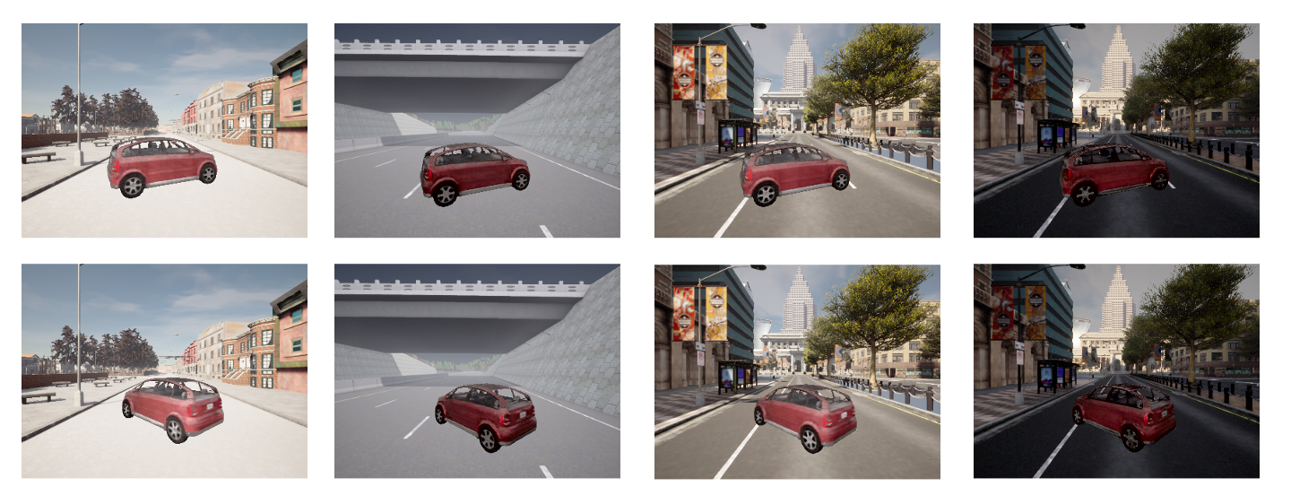
E.1 Number of secondary rays
The LANe architecture that generalizes to unseen scenes requires sampling secondary rays from points on the car to query the light field network for the environment.
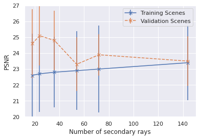
As indicated in Table. 4, the quality of the lighting-aware composition depends on the number of secondary rays sampled. It is natural to expect that the quality improves with an increase in the number of sampled secondary rays. We find that while this is indeed the case in environments observed during training, sampling fewer rays improves lighting-aware composition in unseen environments, as shown in Table 5. Our hypothesis is that the limited capacity of the attention layers causes them to learn an averaged representation of the light field when the number of rays increases. This representation is more biased to the overall lighting of the seen environments and is less sensitive to spatially varying lighting in the unseen environment.
| Num. rays | PSNR | SSIM | FID | LPIPS |
|---|---|---|---|---|
| 144 | 23.4441 | 0.8495 | 0.1742 | 0.1027 |
| 72 | 23.0857 | 0.8467 | 0.1771 | 0.1018 |
| 54 | 22.9917 | 0.8441 | 0.1837 | 0.1038 |
| 36 | 22.8978 | 0.8448 | 0.2081 | 0.1006 |
| 24 | 22.7281 | 0.8437 | 0.2335 | 0.1005 |
| 18 | 22.6449 | 0.8430 | 0.2069 | 0.1004 |
| Num. rays | PSNR | SSIM | FID | LPIPS |
|---|---|---|---|---|
| 144 | 23.5663 | 0.8301 | 0.1321 | 0.1096 |
| 72 | 23.9249 | 0.8340 | 0.1327 | 0.1103 |
| 54 | 23.3989 | 0.8225 | 0.1362 | 0.1154 |
| 36 | 24.8212 | 0.8434 | 0.1136 | 0.1080 |
| 24 | 25.1234 | 0.8439 | 0.1072 | 0.1089 |
| 18 | 24.6220 | 0.8435 | 0.1391 | 0.1017 |
E.2 Number of training environments and generalization
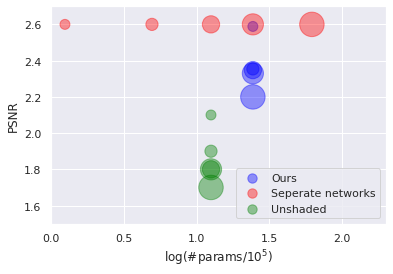
We seek to answer the question - how does increasing the number of training environments affect the performance of the LFN-based shader field on seen and unseen environments? To this end, we train the shader fields on a varying number of environments - 3, 5, 7 - and evaluate them both on an environment used in all the training sets, and a completely unseen environment. We find that increasing the number of environments leads to a slight drop in performance on the training environment (Table 6), but a great increase in performance on the test environment (Table 7).
| Num. train envs | PSNR | SSIM | FID | LPIPS |
|---|---|---|---|---|
| 3 | 22.2764 | 0.8706 | 0.2574 | 0.0975 |
| 5 | 22.2113 | 0.8654 | 0.2274 | 0.0990 |
| 7 | 21.3136 | 0.8593 | 0.3635 | 0.0966 |
| Num. train envs | PSNR | SSIM | FID | LPIPS |
|---|---|---|---|---|
| 3 | 22.4900 | 0.8392 | 0.1551 | 0.1219 |
| 5 | 22.8970 | 0.8514 | 0.1496 | 0.1085 |
| 7 | 24.0604 | 0.8681 | 0.1856 | 0.0968 |
E.3 Number of instances
The shared LANe object model uses a latent embedding to represent multiple car instances. We find that increasing the number of instances only slightly reduces the overall quality of its rendered images for the known-scene object model, keeping model capacity constant. The quality metrics as a function of the number of instances are shown in Table 8.
| Num. instances | PSNR | SSIM | FID | LPIPS |
|---|---|---|---|---|
| 1 | 26.6484 | 0.9501 | 0.1229 | 0.0553 |
| 2 | 24.6540 | 0.8813 | 0.3993 | 0.1085 |
| 3 | 24.0274 | 0.8586 | 0.4580 | 0.1223 |
| 4 | 23.8273 | 0.8474 | 0.5053 | 0.1386 |
| 5 | 23.0509 | 0.8314 | 0.7595 | 0.1630 |
| 6 | 22.7355 | 0.8232 | 0.6089 | 0.1708 |
E.4 Resolution of light field network
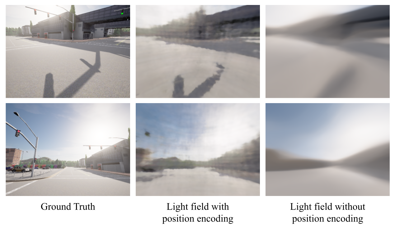
The light field network has been trained to accommodate various lighting requirements using images of the scene at different positions and orientations (Fig 11 for real datasets). The input to this network is a normalized position and ray direction, expressed in Plucker coordinates. The resolution of the light field network depends on the dimensionality of the cosine positional encoding used at the input to the network, higher frequency encodings provide more accurate light fields. When a positional encoding is not used, the light field is very smooth and blurry, and resembles a lighting map of the scene, as shown in Fig 19. We find that the PSNR of the LANe model obtained using light fields with and without position encodings are similar, but using position encodings can sometimes result in periodic shading artifacts. We choose the low-frequency light fields without position encodings for our best-performing model, especially since the light field is queried only in sparse directions and we do not need the precise structure of the world in the lighting information.
E.5 Regressing a multiplicative shading factor vs directly regressing RGB values
The LANe model predicts a shading factor to condition appearance on lighting. An alternative is to directly predict an RGB value from the shader. We find that this performs equally well for single-instance LANe models (Table 9), and is therefore a viable alternative.
| Architecture | PSNR | SSIM | FID | LPIPS |
|---|---|---|---|---|
| Shading factor | 23.4441 | 0.8495 | 0.1742 | 0.1027 |
| Color regression | 23.4813 | 0.8561 | 0.2998 | 0.0957 |
E.6 View-dependent shader
Our shader MLP makes a Lambertian assumption and does not model view-dependent radiance. We evaluate whether including the viewing direction as another input to the shader improves shaded image quality for the real dataset. A comparison of view-dependent shading to view-independent shading is shown in Table 10. We find that the shader is able to model view-dependent effects, and that the rendered image quality is slightly better than the one that does not use view-dependence.
| Model | PSNR | SSIM | LPIPS |
|---|---|---|---|
| View-dep. LANe (LF) | 27.7169 | 0.9408 | 0.0582 |
| LANE (LF) | 26.6371 | 0.9374 | 0.0568 |
Appendix F Relightable NeRF baselines
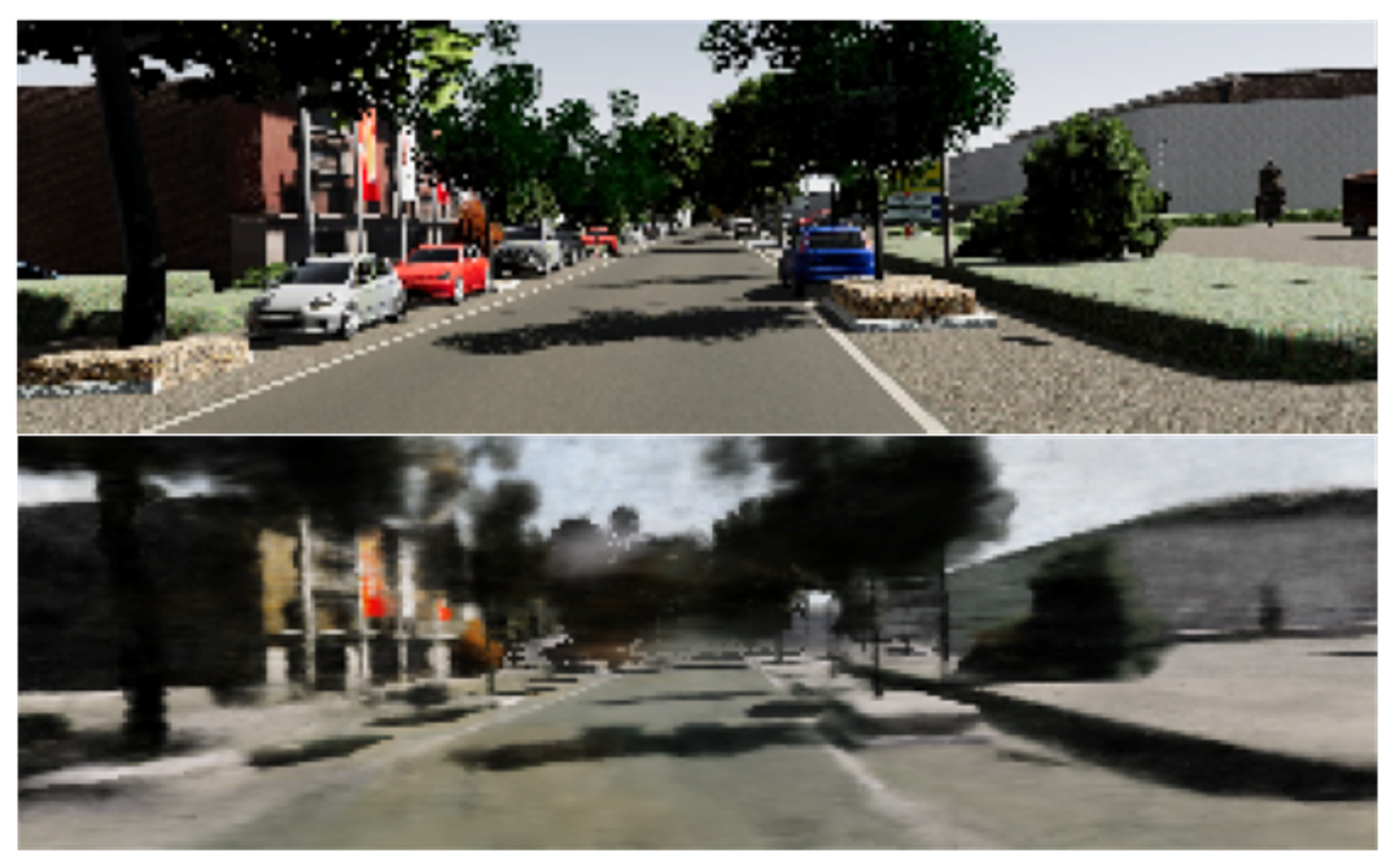
Several recent works [3, 33, 44, 4, 12] have addressed the problem of training relightable NeRF models by decomposing an object’s radiance into its density, material (BRDF), albedo, lighting and visibility mask simultaneously. Such a decomposition is under-constrained and requires additional priors and regularizers. They also make assumptions on light-sources being at infinity, and do not model spatial variance within a scene. They have also not been demonstrated with noisy camera poses or on objects with transparent/translucent objects (such as window shields). Nevertheless, we attempted to compare against one lighting-aware baseline (NeRD [3]). We found that this approach produces very blurry results (Fig 20) on our datasets where the object is not fixed relative to the environment.

Appendix G Limitations
-
1.
Shadow modelling: The LANe model only modulates the appearance of the object with depending on the scene, and does not change the appearance of the scene or other objects after an object has been composed. This implies that effects on the scene (such as the composed object’s shadow) is not modelled.
-
2.
Shadow residuals: As shown in Fig. 18, it is challenging for LANe to cleanly remove existing hard cast shadow of the cars in the foreground, leaving some shadow residuals in the learned world model.
-
3.
The lighting distribution between seen and unseen scenes have to be similar for composition into scenes that the object shader was not trained on.
-
4.
Data requirements: We assume that the same instance was visible in different lighting conditions to train the shader model. This is not true in data collected from real world driving scenarios, where each instance is only captured under lighting changes within the same scene. Training the multi-instance shader model jointly on synthetic instances rendered is several lighting conditions along with real instances observed in different positions in the same scene, could enable it to generalize to unseen real scenes. This is an interesting direction for future work.
Appendix H Societal Impact
With the application of lighting-aware compositional scene synthesis using NeRF, LANe has great potential to be used for data augmentation to train various downstream autonomous driving vision tasks. Specially, the learnt world model and object model could compromise an individual’s privacy and safety, if it has been trained on images containing sensitive information. This is not a concern for the simulated data from CARLA used in our experiments. When releasing our real-world datasets or models trained on it, we intend to mitigate the privacy concern by not including any sensitive information, and blurring information such as people and license plates in our images.