FakET: Simulating Cryo-Electron Tomograms with Neural Style Transfer

Abstract

Particle localization and -classification constitute two of the most fundamental problems in computational microscopy. In recent years, deep learning based approaches have been introduced for these tasks with great success. A key shortcoming of these supervised learning methods is their need for large training data sets, typically generated from particle models in conjunction with complex numerical forward models simulating the physics of transmission electron microscopes. Computer implementations of such forward models are computationally extremely demanding and limit the scope of their applicability. In this paper we propose a method for simulating the forward operator of an electron microscope based on additive noise and Neural Style Transfer techniques. We evaluate the method on localization and classification tasks using one of the established state-of-the-art architectures showing performance on par with the benchmark. In contrast to previous approaches, our method accelerates the data generation process by a factor of 750 while using 33 times less memory and scales well to typical transmission electron microscope detector sizes. It utilizes GPU acceleration and parallel processing. It can be used to adapt a synthetic training data set according to reference data from any transmission electron microscope. The source code is available at https://gitlab.com/deepet/faket.

Keywords— Machine Learning, Deep Learning, CryoET, Cryo-Electron Tomography, Neural Style Transfer, CryoEM, Deep Finder, Synthetic Data Generation, Pre-training, Domain Adaptation, Classification, Localization

Acknowledgement— The IMP and D.H. are generously funded by Boehringer Ingelheim. We thank Julius Berner from the Mathematical Data Science group @ UniVie, Ilja Gubins and Marten Chaillet from the SHREC team, and the members of the Haselbach lab for helpful discussions.

Correspondence to— P. Harar $<$pavol.harar@univie.ac.at$>$ and D. Haselbach $<$david.haselbach@imp.ac.at$>$

1 Introduction

Model	Training data	Data cost	Localization F1	Classification F1
DeepFinder	benchmark	$\approx 150\,h$ (3$\times$CPU, 114 GB RAM)	0.815	0.581 ($100\,\%$)
DeepFinder	faket + fine-tuning	faket cost + manual labeling	0.821	0.565 ($97\,\%$)
DeepFinder	faket	$\approx 12\,m$ (1$\times$GPU, 40 GB VRAM)	0.800	0.533 ($92\,\%$)
DeepFinder	baseline	$\approx 20\,s$ (1$\times$CPU, 1 GB RAM)	0.813	0.441
TM-F			0.576	0.446
TM			0.372	0.470

Table 1: Comparison of DeepFinder’s performance on localization and classification tasks as a function of training data. The performance is evaluated on the same test tomogram. The results are shown in context with the performance of standard template matching algorithms (denoted TM and TM-F) reported in Gubins et al. (2021) for the same testing data. Performance is measured using the F1 score for localization and the F1 macro score for classification. Each of the DF results is an average of the test performances measured at the best epoch (based on validation) over 6 different random seeds. On the challenging classification task, DF trained using faket data simulated by our proposed method reaches 92 % of the performance of DF trained using benchmark data. It even reaches 97 % when fine-tuned using a portion of benchmark data. All this for a fraction of computational cost and without the need for a configuration protocol of the original simulation parameters used for crating benchmark.

Recent developments in cryo-electron tomography (cryoET) allow to obtain high resolution representations of macromolecular complexes in their native cellular environment showing molecular interactions that are hardly accessible with other methods Turk and Baumeister (2020). In cryoET, the imaged sample is in most cases a 100-200 nm thick slice of a frozen cell. From this slice, projection images are taken in a transmission electron microscope (TEM) from different rotation (tilt) angles. An artifact free reconstruction would require measurements using tilt angles, that would complete the half circle. However, this is not feasible, due to limitations of the specimen holder, and only a range of 140^∘ can be recorded. The missing tilt images later on result in a so-called missing-wedge in the 3D reconstruction (cryo-electron tomogram). In addition, the electron beam severely damages the sample during imaging, so only a low electron dose can be used to image a biological specimen. The low dose in combination with the presence of ice in the sample results in the acquired data being very noisy. Consequently, the identification of molecules within these reconstructions is a daunting task. Particle identification is however necessary as the particles need to be classified and averaged to determine high resolution structures. While cryoET has led to a large number of breakthroughs, providing hitherto unseen detail in the molecular architecture of cells (Zimmerli et al., 2021; O’Reilly et al., 2020; Mahamid et al., 2016), the aforementioned challenges still hinder the widespread use of cryoET in the larger cell biology and structural biology community. In this context, the development of new reliable software tools is of paramount importance, which is however obstructed by the lack of sufficient accessible and annotated data to develop the software tools on.

1.1 SHREC simulator

To overcome the problem with the lack of data, in 2019, the annual SHREC – 3D Shape Retrieval Contest included a new track titled Classification in Cryo-Electron Tomograms. The organizers of this track proposed a task of localization and classification of biological particles in cryo-electron tomograms. In the following years, experts from 3D object retrieval and 3D electron microscopy communities were invited to participate in the challenge. In order to ensure fair evaluation and comparable results across the submissions, the organizers created a data set of ten physics-based cryo-electron tomogram simulations (9 train & 1 test tomogram) for the contestants to train and evaluate their methods on. Each year, the results of the contesting methods were presented and compared Gubins et al. (2019, 2020, 2021).

Unfortunately, simulating the tomographic data using SHREC is computationally very expensive. For a set of 10 small tilt-series (61 tilts of size $1024\times 1024$) it took approx. 150 CPU hours of computation on a node with $2\,\times$ Intel Xeon E5-2630 v4 CPUs. The implementation is able to utilize only 3 CPU cores per job in parallel and each job needs 114 GB of RAM. The memory consumption is also a reason why utilizing GPUs and simulating tilt-series of common sizes is not yet feasible (personal communication with the authors Gubins, I., and Chaillet, M.). This limits the scope of its applicability, mainly in data-hungry applications such as deep learning. Moreover, at the time of writing of this article, the source code of the simulator is not publicly available.

1.2 Our contribution

In this paper, we propose faket, a novel method for simulating the forward operator of a cryo transmission electron microscope to generate synthetic tilt-series. It was created, among other reasons, to generate training data for deep neural networks to solve tasks such as particle localization and (much more challenging) particle classification. Our method combines additive noise and neural style transfer (NST) techniques based on Gatys et al. (2016) and is evaluated on downstream tasks using DeepFinder (DF)  Moebel et al. (2021) – a neural network specifically tailored to the task of particle localization and classification, see also Section 4.1.

faket is a surrogate model that mimics the behavior of the physics-based TEM simulator SHREC, while being drastically less computationally expensive, both in terms of time and memory (see Table 1). It also does not require any calibration protocol as other simulators, see Section 1.4. Moreover, it does not need to be retrained to be used on new data, nor does it require labeled reference data. In contrast to SHREC, our method accelerates the data generation process by a factor of 750 while using 33 times less memory. It therefore has the potential to save experts countless hours  of manual work in labeling their data sets.

Moreover, our method is capable of simulating large tilt-series, which are common in experimental environments (about $~{}12\times$ larger than SHREC projections). For example, we generated a $61\times 3500\times 3500$ tilt-series on a single NVIDIA A100 40GB SXM4 GPU in less than 10 minutes. This advance makes it possible to train particle localization and classification networks from scratch, or to pre-train networks that are later fine-tuned using manually labelled experimental data, see Appendix C. On top of that, our method is open source and our experiments are reproducible.

Additionally, we include comparisons of the benchmark and the proposed faket method with a simple baseline method based on additive Gaussian noise, which will be useful for practitioners who need to decide which method fits into their computational budget. The contribution of our method is further supported by an ablation study presented in Appendix D, where we also offer insight into the potential limits of DF on the studied data by conducting experiments using completely noiseless simulated tomograms.

1.3 Related work

A similar idea in X-ray-based computed tomography angiography (CTA) was investigated in Seemann et al. (2020). The authors focused on solving a lumen segmentation task. However, due to the very different nature of the samples imaged in CTA , it was not clear whether a similar NST based framework could be successfully applied in cryoET to image nanoscale particles. In addition, the article does not provide source code and does not document the experiments in enough detail for us to be able to reproduce the results or adapt the method to the cryoET domain.

1.4 Other simulators

The value of simulated data in cryoEM is well recognized and micrograph simulation has been attempted several times. In first approximation a single cryoEM micrograph is the projection of a 3D object, convolved with the electron microscope’s point spread function. Additionally, the overall process comprises several sources of noise coming from the nature of the sample, the microscope, and the imaging procedure which are hard to model accurately. For a better overview of the attempts, it is necessary to mention TEM simulators that were developed in the past decades to simulate micrographs in cryo conditions.

Earlier works provided fast simplistic models mostly based on additive white Gaussian noise or coloured noise Scheible et al. (2021). Other works originated from the insights into the physics of TEM image formation and advanced the simulations by modeling various sources of noise, e.g. an improvement in modeling the structural noise was proposed in TEM Simulator (C) Rullgård et al. (2011). Another improvement was done in InSilicoTEM (Matlab) presented in Vulović et al. (2013) by implementing the multislice method originally proposed in Cowley and Moodie (1957). This makes it the next most relevant simulator related to our work after SHREC which is, as many others, also based on the same multislice method . To the best of our knowledge, the most recent improvement presented in Himes and Grigorieff (2021) is distributed as a part of cisTEM package (C++). It introduced frozen plasmon method to explicitly model spatially variable inelastic scattering processes in cryo-electron microscopy. The aforementioned works, based on the same multislice method, however, suffer from a heavy computational burden or are limited to simulations of a single molecular complex. Despite these limitations, they represent a set of precise advanced physics-based simulators and as such also provide a comprehensive literature survey referring the reader to a body of detailed resources about modeling the image formation in transmission electron microscopy.

In material sciences, GPU accelerated simulators such as MULTEM (C++, CUDA) Lobato and Van Dyck (2015); Lobato et al. (2016), abTEM (Python) Madsen and Susi (2020), or Prismatic (C++, CUDA) Pryor et al. (2017) have emerged. However, as reviewed in Kirkland (2020), advanced TEM simulators used in material sciences require atomic models of the background and the entire specimen. Moreover, in cryoEM, the sample and its interaction with the electron beam is fundamentally different. While in material science samples are often only a few layers of atoms thick and the imaged atoms have strong interaction with the electron beam, cryoEM samples are thousands of atom layers thick, are less ordered, and only weakly interact with the electron beam. Additionally, cryoEM samples can only withstand little radiation before complete destruction resulting in much lower signal to noise ratios. Due to these differences, such simulators are of limited use for macromolecular biological specimen simulations that we experiment with in this article. Finally, in contrary to our approach, all aforementioned methods require precise calibration protocols for setting the values of simulation parameters.

1.5 Structure of this article

To build our proposed method, presented in Section 3 (further referred to as faket), we used a data-driven approach (i.e. no calibration protocol is needed). More information about the data we used is in Section 2. With our method, we managed to successfully approximate the input-output behavior, on par with the SHREC simulator (further referred to as benchmark), but for a fraction of its computational cost. To experimentally prove the need for our method, we also compared it to a simple addition of Gaussian noise (further referred to as baseline) that was naturally very fast to compute, but did not lead to comparable results on the downstream tasks.

To evaluate the methods, we used the simulated data by each of them as a training set for the DeepFinder neural network (more in Section 4.1). The network was trained to solve two evaluation tasks proposed in SHREC challenge. The final comparison was done by observing the models’ performances on the test tomogram chosen by SHREC. Detailed description of the evaluation is in Section 4. More on experiments and results in Section 5. This paper is accompanied with source code, the results are fully-reproducible, and the full experiment results are available in the repository.

Side-by-side comparison of all projections used in this article is available in Appendix A. The process of re-creating the benchmark data is detailed in Appendix B. Fine-tuning experiments that further improved the DF performance are described in Appendix C. Additional experiments, NST ablation study, and investigation of DF limits are presented in Appendix D. Further details on the performance of studied models on the particle classification task are provided in Appendix E.

2 Data

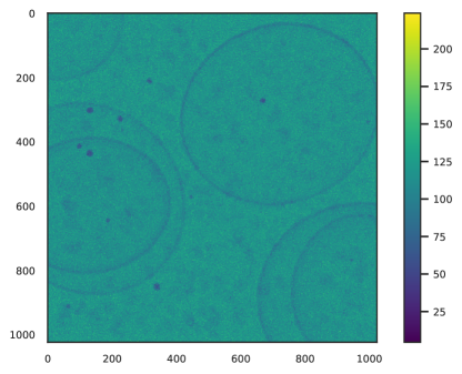
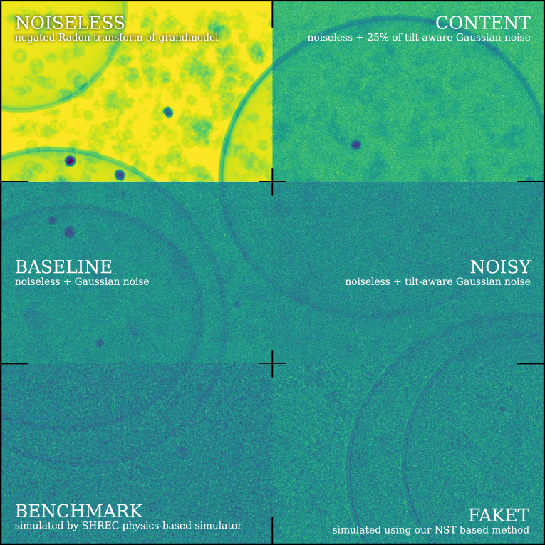
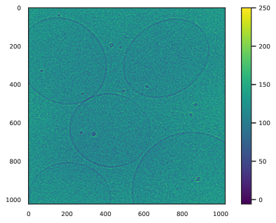
For the purposes of this paper, we used the latest version of the SHREC data set from the year 2021. More specifically, we based the presented methods on full-resolution grandmodels (synthetic volumes containing randomly scattered particles) and simulated projections from the SHREC 2021 additional data set that was made publicly available. An example visualization of a simulated projection using the SHREC simulator is depicted in Figure 1. We use the unchanged simulated projections as a benchmark which we try to approximate with our proposed method.

The steps to create the simulations were described in Gubins et al. (2021). However, at the time of writing of this paper, the implementation is not publicly available and from the description of the steps it is clear that the method is, and rightfully so, very elaborate, and not at all elementary to reimplement (also due to various steps being under-documented, see Appendix B).

Figure 1: Simulated projection from SHREC 2021 data set. Axes x and y correspond to width and height of the imaged grandmodel. Colorbar denotes simulated intensities in arbitrary units. See Appendix A for side-by-side comparison with other projections.

On the following lines, we briefly summarize the steps needed to create the SHREC data set. The authors first constructed 3D ground-truth specimens (grandmodels) along with annotations. Each specimen contained uniformly distributed and rotated protein instances (represented as Coulomb density) of varying size and structure from the Protein Data Bank (PDB) Berman et al. (2000), as well as membranes and gold fiducials, which are commonly found in tomograms. Then, they simulated a layer of amorphous ice into the grandmodels before rotating them over 61 evenly-spaced tilt angles, ranging from -60^∘ to +60^∘, in order to be projected. The noiseless projections were produced using their own implementation of a TEM simulator based on the multislice approach presented in  Vulović et al. (2013). Next, they sampled from a Poisson distribution with a specific electron dose to obtain the final electron counts (files labeled as projections). After that, they randomly shifted the projections to model the tilt misalignment and scaled the amplitudes in Fourier space using information about amplitudes from experimental images in order to increase their similarity (files labeled as projections_unbinned). In the end, they obtained the final images (files labeled as reconstruction) by reconstructing the $2\times$ binned projections using weighted-backprojection algorithm from a private version of the PyTom package Hrabe et al. (2012).

We chose the SHREC data set as it is established, well-executed, downloadable, and allows researchers to compare their results with previous works without the need to reproduce all results from scratch. In this paper, we are not focusing on solving the proposed tasks, instead, we are using them as evaluation metrics to measure the performance of our proposed method. However, the availability of the data and descriptions of the methods made this research feasible.

Figure 2: Noiseless projection used to create the input to our proposed method. Axes x and y correspond to width and height of the imaged grandmodel. Colorbar denotes intensities measured using Radon transform and negated such that particles have lower intensities than the background, as it is in the case of TEM which measures attenuation of electron beams. The particles are not embedded in any solvent (as if they were in vaccuum instead of being embedded in ice), therefore the background appears much brighter than in the simulated projections. See Appendix A for side-by-side comparison with other projections.

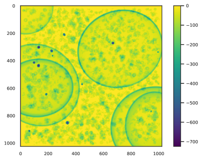
As stated earlier, we used the full-resolution grandmodels from the SHREC data set to create our own noiseless projections using Radon transform, as implemented in the scikit-image library for image processing in Python Van der Walt et al. (2014). We computed our own noiseless projections for three primary reasons. Firstly, SHREC only supplied full-resolution noiseless projections embedded within the simulated ice layer, a feature we also aimed to incorporate in our surrogate. Secondly, we intended to provide access to all implementation steps within the code-base. Lastly, it was necessary to produce noiseless reconstructions that could later be used to estimate the performance boundaries of DF on this data set. We also had to omit the usage of the reconstructions provided by SHREC because the exact configuration of all the steps is not published and the version of the PyTom software package used to create this data is not public. Also, the public version is not yet properly documented or straightforward to use. Thus, the only feasible option to ensure comparable results across our experiments was to create our own reconstructions from all the newly created projections described in Section 3. Nevertheless, we put a lot of effort into matching our reconstructions with the ones originally published in SHREC. We created them using the RadonTea Python package Müller, Paul (2013) using a custom filter described in Appendix B. For additional flexibility, we also implemented support for tomographic reconstructions using the well-known IMOD package Mastronarde and Held (2017). To ensure comparability also with previously published results, we used the original SHREC model_9 reconstruction as a test tomogram for all presented methods as it was done in all the past challenges.

Figure 3: baseline projections. Axes x and y correspond to width and height of the imaged grandmodel. Colorbar denotes simulated intensities in arbitrary units. Please note that this projection is not exactly the same as in Figure 1 or in Figure 4, see also the explanation in the caption of Figure 4 and Appendix A for a side-by-side comparison with other projections.

3 Methods

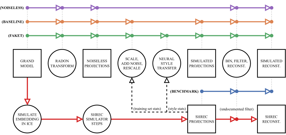
The methods described in this section represent surrogate models that mimic the behaviour of the aforementioned SHREC physics-based simulator. The methods are to be applied in the projection space, i.e. all of them take noiseless (and ice-less) projections as inputs, shown in Figure 2, and produce real-like looking projections by matching their appearance with a target “style” projections. The outputs are ready to be reconstructed into final tomogram volumes using a reconstruction algorithm of choice. There are multiple reasons why we decided, and why it is reasonable, to model the simulator’s behaviour in projection space. Firstly, different reconstruction algorithms produce different types of artifacts and are suitable in different situations. Therefore, simulating only projections means the models do not have to mimic the artifacts crated by the reconstruction algorithm (e.g. smearing due to the missing wedge). Moreover, this approach does not limit the practitioners in their choice of the reconstruction algorithm, and opens the possibility for researchers to also use the methods in research of novel reconstruction algorithms. But most importantly, simulating in projection space means the models need to process and produce an order-of-magnitude less data points, as compared to simulating the final reconstruction volumes. That means, simulating $\theta\times N^{2}$ data points instead of $N^{3}$. In our case, $\theta=61$ and $N=1024$. In practice, $\theta$ stays approximately the same, but $N$ is usually 3 – 4$\times$ larger.

Figure 4: faket projections. Axes x and y correspond to the grandmodel’s width and height respectively, and colorbar indicates simulated intensities in arbitrary units. While this projection may appear visually similar to Figure 3, there is a subtle difference that has a significant impact on DF’s performance. This similarity complicates comparison of projections from various simulators using currently available image metrics. See Appendix A for a side-by-side comparison with other projections.

3.1 Additive noise (baseline)

Before moving on to the development of more complicated methods, we wanted to see how a very simple method involving tilt-dependent scaling and the addition of Gaussian noise would approximate the target projections. The modality of projections produced by this method is referred to as baseline projections in the whole text. First, we shifted and scaled each tilt of the noiseless input projections separately according to the average mean and standard deviation of each tilt within the training set. Through this tilt-dependent scaling, we attempt to model different degrees of attenuation as a function of tilt angle - the more extreme the tilt angle, the greater the attenuation due to the longer electron beam trajectory.

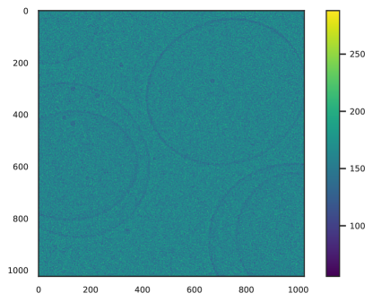
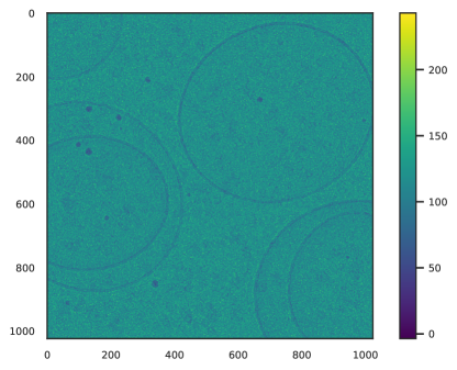
Next, we simply add Gaussian noise, as this is the natural choice of practitioners when they need to quickly create some simulated tilt-series. Of course, this raises the question of how much noise to add. In reality, practitioners would probably visually choose a value for $\sigma$ that gives a similar signal-to-noise ratio. However, we opted for a more objective procedure by subtracting the noiseless content from the target projections to extract the noise and measure its statistics. With SHREC data, where precise ground truth is available, this task is less challenging than with real data, where we lack ground truth for the entire tomogram. So in a real scenario we would have to select regions for which we can estimate the ground truth and calculate the noise statistics only for these regions instead of using the whole tilt values. After adding the Gaussian noise, the resulting volume was scaled to match the average mean and standard deviation of the training set with respect to tilt. The steps for creating projections and consequently reconstructions using this method are shown in Figure 5, and an example of a simulated projection can be seen in Figure 3. The calculation of this modality takes only a few seconds using a single CPU.

Figure 5: Diagram of steps to simulate the benchmark, baseline, faket, and noiseless projections and reconstructions. Red arrows highlight steps to reproduce SHREC data from which we use the last tomogram for testing. All methods except SHREC were filtered using a reverse-engineered filter (see Appendix B) because the SHREC filtering step is under-documented. The style projections never feature the same contents as the simulated ones (see Appendix A).

3.2 Neural Style Transfer (faket)

To capture the noise structure of the benchmark projections more closely, in faket we devised a more elaborate method of estimating the noise statistics as opposed to the simpler one used in baseline. In this case, we estimate the noise statistics for each tilt in the whole training set separately and fit a second-degree polynomial over the averages. This process captures the average noise statistics as a function of tilt angle based on the information from the whole training set. After adding the better estimated Gaussian noise, we obtained projections which we will refer to as noisy projections. To further adapt those projections, we used the Neural Style Transfer technique implemented in PyTorch framework Paszke et al. (2019) and introduced in Gatys et al. (2016).

NST was built to render the semantic content of natural images in different styles. At its core lies VGG net Simonyan and Zisserman (2014), a convolutional neural network optimized for object recognition and -localization. Within the NST framework, the VGG net is used for extracting the content and style representations of so-called “content” and “style” images, which are provided as inputs. NST then iteratively updates the output image to simultaneously match the content representation and the style representation of the provided inputs at multiple scales. NST is described in the aforementioned paper in great detail and we encourage the reader to consult it if any questions would arise.

Cryo-electron projections are not natural images as those used to pre-train the VGG net. It would be therefore surprising if the NST provided us with desired results “out-of-the-box”. The first experiments with NST using the noiseless projections as content images and benchmark projections as style images were disappointing due to numerous strong artifacts scattered apparently randomly over the adapted projections. Search over the space of hyper-parameters did not result in satisfactory output even after 10 thousand iterations. Further experiments with baseline projections as content images performed poorly on the evaluation task, especially on localization of smaller particles. It might be useful for the readers to know that before we even decided to work in projection space, our very first experiments were done in reconstruction space, but this idea had to be quickly abandoned due to the poor performance, failure to transfer the artifacts of reconstruction algorithm and computational infeasibility.

In order to obtain the desired results, we adjusted the NST to our specific needs. Firstly, we adjusted the code to accept sequences of 1-channel floating point arrays as inputs to improve the speed of processing. Next, we rid the code of conversions associated with handling RGB images in order to preserve the floating point precision of our data. And finally, we implemented the support for other than random initialization or initialization with the content which was a crucial change to produce the desired results. We initialized the NST with noisy projections, used noisy projections with 25 % of noise as content, and provided the associated benchmark projections as style images. We would like to point out that the associated style images were taken from a different training tomogram, therefore do not feature the same content. I.e. it is not possible to simply minimize the element-wise mean absolute error to get the desired output.

From the NST pipeline, we only used the 1024x1024 scale because downsampling to smaller scales combined with anti-aliasing used in NST to transition between the scales is well suited for natural images and lots of NST iterations but not for our use case on scientific data. Using new initialization and slightly noisy content images allowed us to increase the learning rate of the NST optimizer, so we were able to produce visually persuasive outputs in just one iteration, as seen in Figure 4.

This method is more involved than just adding the noise, but produces better results, is very fast due to our changes of NST initialization and hyper-parameters, requires less domain-specific knowledge than implementing the forward operator, and can be used in real-world scenarios. Computing this modality of data, including the steps to create the noisy projections and content projections for 10 tomograms took only $\approx$12 minutes on a single NVIDIA A100 40GB SXM4 GPU, which on average represents a $750\times$ speedup in comparison to benchmark. This method also needed only $\approx$3.5 GB of GPU memory per tomogram as opposed to 117GB of RAM which was necessary for benchmark. The GPU memory usage of our method could be even further optimized. This represents 33 times less memory usage. Certainly, it is not possible to do a head-to-head comparisons between GPU memory and RAM, but this information can be used to estimate the hardware requirements. Moreover, as opposed to the benchmark method, it is possible to scale our method to volumes that match usual sizes of experimental data on still reasonable hardware.

4 Evaluation

To evaluate the quality of the proposed simulated projections and subsequently tomograms, no widely accepted metrics exist Seemann et al. (2020), and it is not clear how well the standard metrics such as the mean squared error, or more elaborate metrics such as the Fréchet inception distance Heusel et al. (2017), relate to the performance on tasks of interest to the practitioners.

We therefore trained a randomly initialized DF neural network to solve two evaluation tasks proposed in the SHREC 2021 challenge, namely particle localization and classification. These tasks are of utmost importance to practitioners in determining the structure of proteins and macromolecular complexes. We argue that evaluation on a task of practical relevance is much more valuable than merely computing the currently available metrics. It also gives the reader an advantage to see the newly created data modalities in practice, even though the computational cost of evaluation is high.

To obtain the main results, we trained DF for 70 epochs on benchmark, faket, and baseline training data, every time across 6 different seeds of randomness ($3\times 6$ times in total). Each model was tested on the same test tomogram – model_9 from the original SHREC data set. The final comparison was done by observing the models’ performances in terms of F1 score for localization task and F1 macro score for classification task. The computation of the scores was done the same way as in Gubins et al. (2021) where also further particularities of the tasks are described. To estimate the 68 % and 95 % confidence intervals, we used the bootstrapping method. The results are visualized and discussed in Section 5. Results of additional experiments are presented in the Appendix.

4.1 DeepFinder

DeepFinder emerged from the SHREC challenge as one of the most successful candidates. One other reason why we chose to use DF was the availability of its source code. DF is a deep 3D-convolutional neural network trained in a supervised fashion by optimizing a dice loss. For training of the models, we used the Adam optimizer with learning rate of $0.0001$. The exponential decay rate was set to $0.9$ for the first moment estimate and $0.999$ for the second moment estimate as in Moebel et al. (2021).

To train the DF, we used tomograms containing particle instances from 16 classes (two of those being background and vesicles). We adjusted the training procedure of DF such that in one epoch, all patches containing particles within the training data set were seen once, or with minimal repetition. a patch in a shape of a box is rotated by 180^∘ at random. Patches are processed in batches constructed from a randomly permuted list of all particles in the training set. After our changes in the training procedure, an epoch represents a different number of gradient steps than in Moebel et al. (2021), therefore the numbers of epochs are not comparable with the original paper. To perform the particle localization and -classification on the test tomogram, DF carries out a segmentation procedure followed by clustering and thresholding steps, where the two latter steps are computed using a CPU. The thresholding is used to reduce the number of false positive findings.

Figure 6: Performance on localization task.

To train the DF network implemented in Keras framework Chollet et al. (2015) using TensorFlow backend Abadi et al. (2015), we utilized multiple NVIDIA A100 40GB SXM4 GPUs. That allowed us to run multiple experiments in parallel. One training job comprising of 9 training tomograms required approx. 17GB of GPU memory, therefore we were able to submit two jobs on one GPU at a time. One training epoch, as defined earlier, took $\approx$21 min. to finish. The segmentation of a test tomogram took $\approx$2.5 min. on the aforementioned GPU. The clustering step took $\approx$30 min. on a single core of a $2\times$ 64-core AMD EPYC 7742 CPU. The most computational expensive step was thus the training of the DF.

5 Results

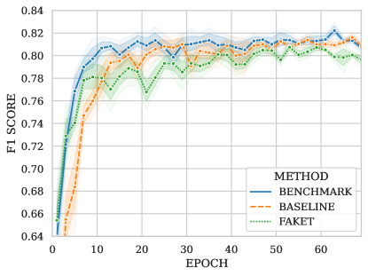
Comparison of DeepFinder’s performance on localization and classification tasks as a function of training data is presented in Table 1. The mean performances per epoch with 68 % and 95 % confidence intervals (CI) are presented in Figure 6 and Figure 7. Results of additional experiments can be found in Appendices C, LABEL:, D, LABEL: and E.

The performance of DF trained on benchmark data turned out to be the best in both localization and classification tasks, as expected, since the testing tomogram was reconstructed from the exactly same tilt-series as benchmark training set. In practice, however, it is infeasible to have such favorable conditions as fully labelled tomograms are not existent. Most biological studies focus on one or a subset of molecules to be labelled. And since the labelling process is laborious and requires domain experts, it is also expensive. With that in mind, we can hardly expect to have a training set of tomograms from exactly the same distribution as the tomograms we are interested in. Nevertheless, this result serves us, as the name suggests, as a benchmark that we are trying to reach with our proposed methods.

The highest benchmark F1 score of 81.5 % (68 % CI [81.1 %, 82.0 %]) on localization task and 58.1 % (68 % CI [57.9 %, 58.3 %]) on classification task on average across 6 different random seeds was achieved after 65$\pm$4 epochs of training.

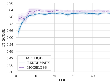
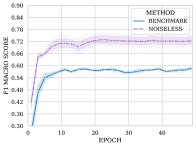
To put these numbers in perspective, we investigated the limits of DF performance by training and evaluating on completely noiseless data, see Appendix D for more details. In this setting DF achieved F1 score of 83.2 % (68 % CI [82.4 %, 84.0 %]) on localization task and 72.5 % (68 % CI [70.5 %, 74.6 %]) on classification task.

Figure 7: Performance on classification task.

Figure 8: Per-class performance on classification task.

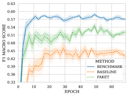
Our fastest method of simulating the projections and subsequently the tomograms, baseline, scored 81.3 % (68 % CI [81.1 %, 81.6 %]) on localization task. It was a surprise that such a simple method led to so high localization performance, considering that it requires $\approx 150\,h$ to create the benchmark projections, while it takes almost no time to create the baseline projections. This method can be therefore regarded as the “poor-man’s” choice in settings where the computational budget is very limited, or in settings where this task has to be performed repeatedly many times. Unfortunately, the classification performance of 44.1 % (68 % CI [43.2 %, 45.1 %]) was rather poor, not surprisingly, as classification is an inherently harder task, cf. Gubins et al. (2021).

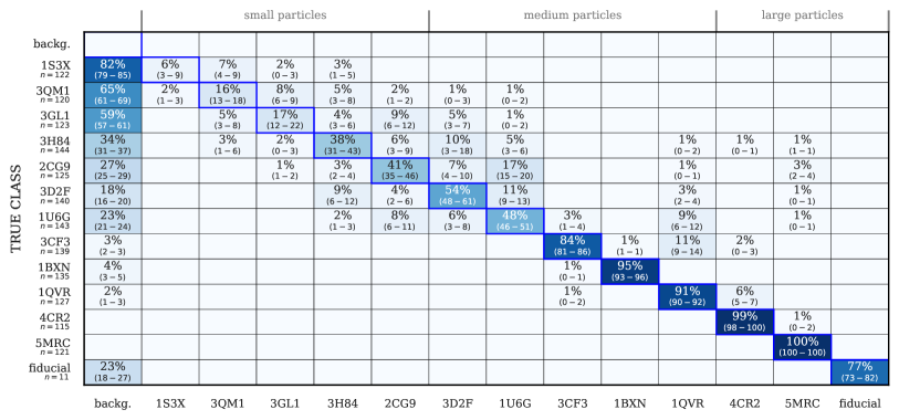
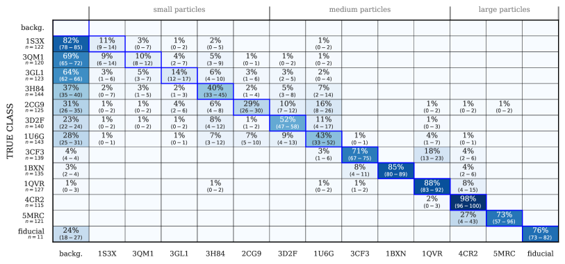
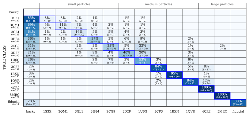
Our proposed method faket, based on additive noise (using our advanced estimation of in-projections noise) and subsequently neural style transfer, with on average 80.0 % (68 % CI [79.8 %, 80.2 %]) F1 score on localization task performed on par with the benchmark and significantly outperformed standard template matching algorithms. The best performance on the classification task was achieved after 65$\pm$4 epochs with a score of 53.3 % (68 % CI [52.8 %, 53.8 %]). With this result, faket matched the benchmark to 92 % while reducing the cost of data generation by a factor of 750 and using 33 times less memory. Multi-class classification performance certainly can not be reduced only to one number and it is important to consider also other metrics, such as per-class classification report and confusion matrices. The per-class classification performance is shown in Figure 8 and we provide the confusion matrices in Appendix E. The full performance reports are available in the accompanying repository for enthusiastic readers.

In Appendix C, we present further experimental results showcasing the fine-tuning of faket models using a subset of benchmark data. This approach further narrows the performance gap between the faket and benchmark models, achieving 97 % of the benchmark model’s classification performance, while exceeding its performance on localization task. These results might be valuable for cryoET practitioners who are seeking to maximize the performance of their models and have, or can get a small but representative sample of their data labeled.

6 Conclusions

In this paper, we proposed faket, a method for simulating the forward operator of an electron microscope based on additive noise and Neural Style Transfer. The proposed method can be used for generating synthetic cryo-electron tilt-series which can be used to train deep neural networks to solve tasks such as particle localization and (much more challenging) particle classification. The field of cryo-electron tomography currently suffers from the lack of sufficient amounts of annotated data, and the proposed method aims to solve this problem. faket is a surrogate model that mimics the behavior of the physics-based TEM simulator SHREC, while being drastically less computationally expensive, both in terms of time and memory. It accelerates the data generation process by a factor of 750 while using 33 times less memory, making the generation of thousands of tilt-series feasible. Moreover, it is capable of simulating large tilt-series, which are common in experimental environments. For example, we generated a $61\times 3500\times 3500$ tilt-series on a single NVIDIA A100 40GB SXM4 GPU in less than 10 minutes. It also does not require any calibration protocol, it does not need to be retrained to be used on new data, nor does it require labeled reference data. The method is open source, and the experiments are reproducible.

The quality of our approximations was evaluated using the DeepFinder network, which emerged from the SHREC challenge as one of the most successful. The results showed that the performance of models trained using our approximations is on par with the benchmark method on localization task and reached 92 % of its performance on classification task while significantly outperforming standard template matching algorithms. When further fine-tuned using a portion of benchmark data, the classification performance was improved to 97 %. This advancement simplifies the generation of fully-labeled, high-quality synthetic tilt-series that resemble experimental TEM data requiring analysis. This simulated data can either be used to train particle localization and classification neural networks from scratch, or serve as fpre-training data for networks that will be fine-tuned with manually labeled experimental data later. Researchers investigating reconstruction algorithms can also benefit from our simulator since the availability of ground truth allows for effortless evaluation of their novel methods.

In future work, we will focus on further validation of our method using experimental data from TEM and we hope this advancement will serve as the basis for more method development in cryoET. Additionally, we plan to improve the method by using state-of-the-art neural networks and we want to provide the community of practitioners with a fully functional and easy-to-use piece of software to generate their synthetic data sets based on chosen particles from Protein Data Bank. The goal is to enable more accurate and efficient data analysis while also making the process more accessible to researchers in the field.

Appendix A Side-by-side comparison of projection types

Figure 9: Side-by-side comparison of all different types of projections presented in this article.

(a)

(b)

Figure 10: One instance of style projections (from benchmark) used as a reference for NST (left) and the difference between one particular instance of faket and benchmark projections. Note that the style projection used as a reference input to NST never features the same content as the input projection that is being style-transferred.

Appendix B Recreating benchmark – reverse-engineering SHREC filtering step

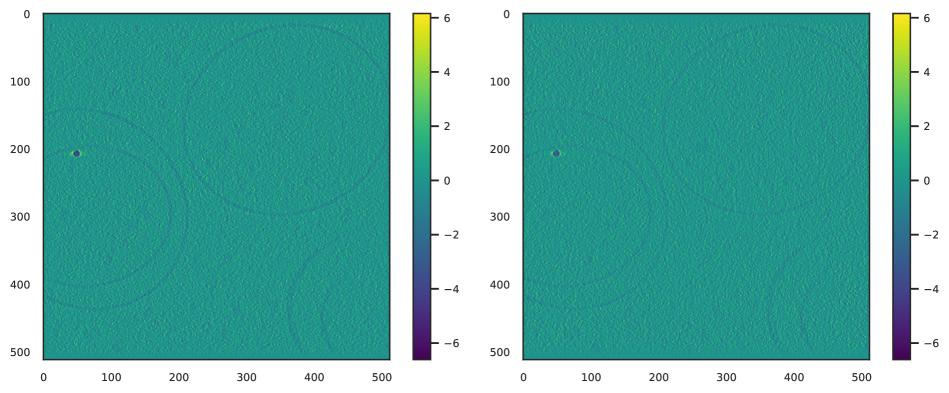
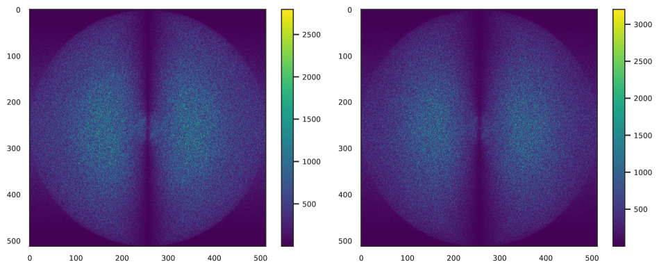
In pursuit of re-creating the benchmark reconstructions to match those from SHREC data set as closely as possible, we inspected the public source code of PyTom Hrabe et al. (2012) for clues on which filters might have been used. In the original paper, authors only mention that they use weighted back-projection. Which would suggest the use of a simple ramp filter. In a personal communication, they mentioned using a default filter from their private PyTom version with undefined Crowther frequency. Therefore, we implemented and used a simple ramp filter with a support for Crowther frequency. Then, we visualized SHREC’s and our reconstructions in Fourier space to visually compare the results. Unfortunately, none of the variations of a simple ramp filter, even with Crowther frequency, produced the expected result similar to SHREC. For that reason, we started to iteratively change our filter in order to approximately match the aforementioned reconstructions in both real and Fourier space, in hope of finding the desired match. After many iterations, we found a good-enough match, a filter which is a product of a 2D Gaussian filter ($\sigma_{x}=174$, $\sigma_{y}=102$), a 1D ramp filter broadcasted to 2D ($\mathrm{CrowtherFreq}=0.61$ Nyquist), and a 2D circular filter ($\mathrm{radiusCutoff}=256$, i.e. Nyquist frequency). Exact implementation is available in code repository.

(a) Reconstruction space

(b) Fourier space

Figure 11: Middle Z-axis slice of SHREC (left) and benchmark (right) reconstructions.

Appendix C Further improving the performance of DF models trained with faket data by subsequent fine-tuning on a fraction of benchmark data

Fine-tuning is a prevalent approach in machine learning where a pre-trained model is further refined using a subset of the available data specific for the task. This methodology often yields improved performance by allowing the model to specialize on the nuances of a specific dataset. For practitioners in cryoET, this process can be of great value when seeking to maximize the performance of their models. If they are able to label a small but representative sample of their data manually, they can leverage this technique to their advantage.

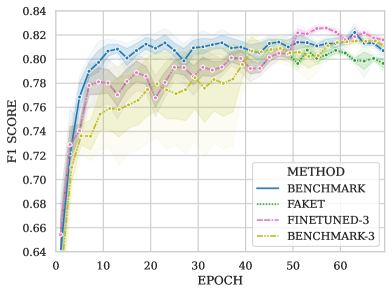
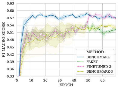
Here, we compared the performance of models trained on baseline or faket data with that of a model initially trained on faket data and later fine-tuned using a subset (3 out of 9) of benchmark tomograms, denoted as finetuned-3 in the figures. The fine-tuning began after the 50^th epoch, triggering a notable improvement in both localization and classification performance. To make a reasonable comparison, we include results from a model, benchmark-3, trained solely on the same 3 benchmark tomograms used for fine-tuning.

During the fine-tuning and benchmark-3 training stages, the total number of training tomograms was smaller. To maintain experiment consistency by keeping an approximately equivalent number of gradient steps per epoch, we adapted our definition of an epoch. Here, it refers to a cycle where the model is trained on 9 tomograms — meaning that during fine-tuning, three full training cycles with 3 tomograms each are considered one epoch.

(a) Performance on localization task

(b) Performance on classification task

(c) Per-class performance on classification task

Figure 12: Performance of finetuned-3 and benchmark-3 models in context with the main results.

Appendix D Additional experiments

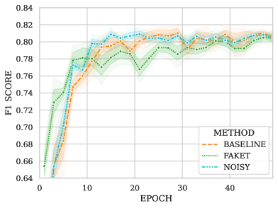
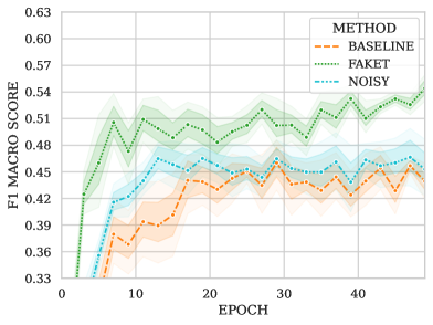
For our baseline, we chose the conventional approach of adding Gaussian noise. However, acknowledging the noise component in TEM projections fluctuates with tilt angle, we devised a tilt-dependent algorithm for Gaussian noise addition. This formed the basis for our NST-based faket method, producing what we refer to as noisy projections. One might wonder if such simulation enhances DF performance, a query best illustrated by a figure. Although localization performance remained consistent, we observed a slight enhancement in classification, as shown in Figure 13 (top). Despite this modest improvement, we didn’t deem it significant enough to modify our simple baseline method, but still opted to incorporate it into our faket method.

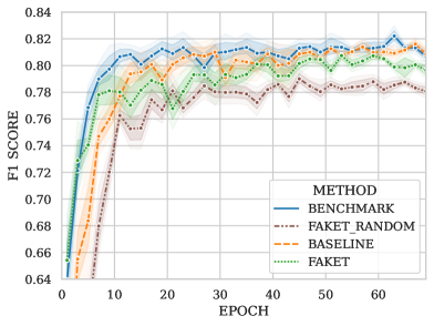
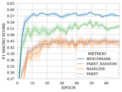
We present an ablation study featuring a faket-random model trained on data created with a randomly initialized NST network, in contrast to pre-trained. Results in Figure 13 (middle) underscore the necessity of pre-training for successful simulation and suggest that pre-training using cryoET data might further enhance the simulated data’s resemblance to real tomograms — a question still under exploration.

Finally, to offer insight into the potential limits of DF on the studied data, we share results from a noiseless experiment in Figure 13 (bottom). The model was trained and tested on completely noiseless reconstructions, making it also the only model in this paper evaluated on a noiseless test tomogram.

(a)

(b)

(c)

(d)

(e)

(f)

Figure 13: Performance of DF trained with noisy (top), faket-random (middle), and noiseless (bottom) data. Localization results are shown in the left column and classification results in the right column.

Appendix E Further details on particle classification performance

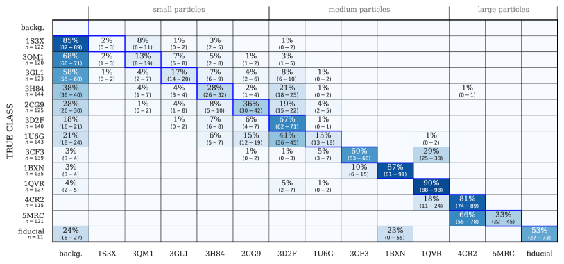
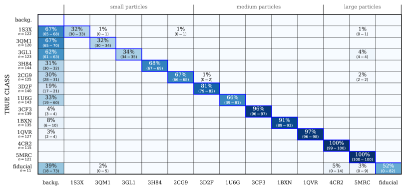
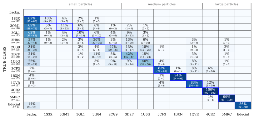
Next to F1 scores reported in Section 5, here we present aggregated confusion matrices for all main and selected additional experiments. Each confusion matrix represents the average of 6 confusion matrices obtained from 6 different experiments each initialized with a different random seed. Each confusion matrix was computed based on the results of the best epoch that was selected based on the model’s validation performance. The csv files containing information about which epochs were selected for each of the aggregated confusion matrices are available in the accompanying repository.

Particles on X and Y axes are sorted according to their volume from the smallest on the left (or top) to the largest on the right (or bottom). Particles are also grouped into size-groups so the reader can get a better feeling for the relationship between particle volume and DF performance. The values at the diagonal represent the fraction of correctly classified particles for a class at any given row. The values in parentheses in each cell show $10^{th}$ and $90^{th}$ percentiles, since the displayed values are averages. The values that are not at the diagonal represent the fraction of the particles that were misclassified as a member of the class at the particular column. The sum of all values in one row is therefore equal to 100 %. Tick labels of the Y axis additionally contain information about the total number of instances of each class within the test tomogram.

(a)

(b)

Figure 14: Aggregated confusion matrices for benchmark (top) and faket (bottom) experiments.

(a)

(b)

Figure 15: Aggregated confusion matrices for baseline (top) and noiseless (bottom) experiments.

(a)

(b)

Figure 16: Aggregated confusion matrices for finetuned-3 (top) and benchmark-3 (bottom) experiments.

References

- Abadi et al. (2015) M. Abadi, A. Agarwal, P. Barham, E. Brevdo, Z. Chen, C. Citro, G. S. Corrado, A. Davis, J. Dean, M. Devin, S. Ghemawat, I. Goodfellow, A. Harp, G. Irving, M. Isard, Y. Jia, R. Jozefowicz, L. Kaiser, M. Kudlur, J. Levenberg, D. Mané, R. Monga, S. Moore, D. Murray, C. Olah, M. Schuster, J. Shlens, B. Steiner, I. Sutskever, K. Talwar, P. Tucker, V. Vanhoucke, V. Vasudevan, F. Viégas, O. Vinyals, P. Warden, M. Wattenberg, M. Wicke, Y. Yu, and X. Zheng. TensorFlow: Large-scale machine learning on heterogeneous systems, 2015. URL https://www.tensorflow.org/. Software available from tensorflow.org.
- Berman et al. (2000) H. M. Berman, J. Westbrook, Z. Feng, G. Gilliland, T. N. Bhat, H. Weissig, I. N. Shindyalov, and P. E. Bourne. The Protein Data Bank. Nucleic Acids Research, 28(1):235–242, 01 2000. ISSN 0305-1048. doi:10.1093/nar/28.1.235.
- Chollet et al. (2015) F. Chollet et al. Keras. https://keras.io, 2015.
- Cowley and Moodie (1957) J. M. Cowley and A. F. Moodie. The scattering of electrons by atoms and crystals. i. a new theoretical approach. Acta Crystallographica, 10(10):609–619, 1957. doi:10.1107/S0365110X57002194.
- Gatys et al. (2016) L. A. Gatys, A. S. Ecker, and M. Bethge. Image style transfer using convolutional neural networks. In Proceedings of the IEEE Conference on Computer Vision and Pattern Recognition (CVPR), June 2016. doi:10.1109/CVPR.2016.265.
- Gubins et al. (2019) I. Gubins, G. v. d. Schot, R. C. Veltkamp, F. Förster, X. Du, X. Zeng, Z. Zhu, L. Chang, M. Xu, E. Moebel, A. Martinez-Sanchez, C. Kervrann, T. M. Lai, X. Han, G. Terashi, D. Kihara, B. A. Himes, X. Wan, J. Zhang, S. Gao, Y. Hao, Z. Lv, X. Wan, Z. Yang, Z. Ding, X. Cui, and F. Zhang. Classification in Cryo-Electron Tomograms. In S. Biasotti, G. Lavoué, and R. Veltkamp, editors, Eurographics Workshop on 3D Object Retrieval. The Eurographics Association, 2019. ISBN 978-3-03868-077-2. doi:10.2312/3dor.20191061.
- Gubins et al. (2020) I. Gubins, M. L. Chaillet, G. van der Schot, R. C. Veltkamp, F. Förster, Y. Hao, X. Wan, X. Cui, F. Zhang, E. Moebel, X. Wang, D. Kihara, X. Zeng, M. Xu, N. P. Nguyen, T. White, and F. Bunyak. Shrec 2020: Classification in cryo-electron tomograms. Computers & Graphics, 91:279–289, 2020. ISSN 0097-8493. doi:10.1016/j.cag.2020.07.010.
- Gubins et al. (2021) I. Gubins, M. L. Chaillet, G. v. d. Schot, M. C. Trueba, R. C. Veltkamp, F. Förster, X. Wang, D. Kihara, E. Moebel, N. P. Nguyen, T. White, F. Bunyak, G. Papoulias, S. Gerolymatos, E. I. Zacharaki, K. Moustakas, X. Zeng, S. Liu, M. Xu, Y. Wang, C. Chen, X. Cui, and F. Zhang. SHREC 2021: Classification in Cryo-electron Tomograms. In S. Biasotti, R. M. Dyke, Y. Lai, P. L. Rosin, and R. C. Veltkamp, editors, Eurographics Workshop on 3D Object Retrieval. The Eurographics Association, 2021. ISBN 978-3-03868-137-3. doi:10.2312/3dor.20211307.
- Heusel et al. (2017) M. Heusel, H. Ramsauer, T. Unterthiner, B. Nessler, and S. Hochreiter. Gans trained by a two time-scale update rule converge to a local nash equilibrium. In I. Guyon, U. V. Luxburg, S. Bengio, H. Wallach, R. Fergus, S. Vishwanathan, and R. Garnett, editors, Advances in Neural Information Processing Systems, volume 30. Curran Associates, Inc., 2017. URL https://proceedings.neurips.cc/paper/2017/file/8a1d694707eb0fefe65871369074926d-Paper.pdf.
- Himes and Grigorieff (2021) B. Himes and N. Grigorieff. Cryo-tem simulations of amorphous radiation-sensitive samples using multislice wave propagation. IUCrJ, 8(6):943–953, 2021. doi:10.1107/S2052252521008538.
- Hrabe et al. (2012) T. Hrabe, Y. Chen, S. Pfeffer, L. Kuhn Cuellar, A.-V. Mangold, and F. Förster. Pytom: A python-based toolbox for localization of macromolecules in cryo-electron tomograms and subtomogram analysis. Journal of Structural Biology, 178(2):177–188, 2012. ISSN 1047-8477. doi:10.1016/j.jsb.2011.12.003. Special Issue: Electron Tomography.
- Kirkland (2020) E. J. Kirkland. Advanced Computing in Electron Microscopy. Springer Nature, 2020. doi:10.1007/978-3-030-33260-0.
- Lobato and Van Dyck (2015) I. Lobato and D. Van Dyck. Multem: A new multislice program to perform accurate and fast electron diffraction and imaging simulations using graphics processing units with cuda. Ultramicroscopy, 156:9–17, 2015. doi:10.1016/j.ultramic.2015.04.016.
- Lobato et al. (2016) I. Lobato, S. Van Aert, and J. Verbeeck. Progress and new advances in simulating electron microscopy datasets using multem. Ultramicroscopy, 168:17–27, 2016. doi:10.1016/j.ultramic.2016.06.003.
- Madsen and Susi (2020) J. Madsen and T. Susi. abtem: ab initio transmission electron microscopy image simulation. Microscopy and Microanalysis, 26(S2):448–450, 2020. doi:10.1017/S1431927620014701.
- Mahamid et al. (2016) J. Mahamid, S. Pfeffer, M. Schaffer, E. Villa, R. Danev, L. K. Cuellar, F. Förster, A. A. Hyman, J. M. Plitzko, and W. Baumeister. Visualizing the molecular sociology at the HeLa cell nuclear periphery. Science, 351(6276):969–972, Feb 2016. doi:10.1126/science.aad8857.
- Mastronarde and Held (2017) D. N. Mastronarde and S. R. Held. Automated tilt series alignment and tomographic reconstruction in imod. Journal of structural biology, 197(2):102–113, 2017. doi:10.1016/j.jsb.2016.07.011.
- Moebel et al. (2021) E. Moebel, A. Martinez-Sanchez, L. Lamm, R. D. Righetto, W. Wietrzynski, S. Albert, D. Larivière, E. Fourmentin, S. Pfeffer, J. Ortiz, W. Baumeister, T. Peng, B. D. Engel, and C. Kervrann. Deep learning improves macromolecule identification in 3d cellular cryo-electron tomograms. Nature Methods, 18:1386–1394, 2021. doi:10.1038/s41592-021-01275-4.
- Müller, Paul (2013) Müller, Paul. radontea: Python algorithms for the inversion of the radon transform, 2013. URL https://pypi.python.org/pypi/radontea/.
- O’Reilly et al. (2020) F. J. O’Reilly, L. Xue, A. Graziadei, L. Sinn, S. Lenz, D. Tegunov, C. Blötz, N. Singh, W. J. H. Hagen, P. Cramer, J. Stülke, J. Mahamid, and J. Rappsilber. In-cell architecture of an actively transcribing-translating expressome. Science, 369(6503):554–557, 07 2020. doi:10.1126/science.abb3758.
- Paszke et al. (2019) A. Paszke, S. Gross, F. Massa, A. Lerer, J. Bradbury, G. Chanan, T. Killeen, Z. Lin, N. Gimelshein, L. Antiga, A. Desmaison, A. Kopf, E. Yang, Z. DeVito, M. Raison, A. Tejani, S. Chilamkurthy, B. Steiner, L. Fang, J. Bai, and S. Chintala. Pytorch: An imperative style, high-performance deep learning library. In Advances in Neural Information Processing Systems 32, pages 8024–8035. Curran Associates, Inc., 2019. URL http://papers.neurips.cc/paper/9015-pytorch-an-imperative-style-high-performance-deep-learning-library.pdf.
- Pryor et al. (2017) A. Pryor, C. Ophus, and J. Miao. A streaming multi-gpu implementation of image simulation algorithms for scanning transmission electron microscopy. Advanced structural and chemical imaging, 3:1–14, 2017. doi:10.1186/s40679-017-0048-z.
- Rullgård et al. (2011) H. Rullgård, L.-G. Öfverstedt, S. Masich, B. Daneholt, and O. Öktem. Simulation of transmission electron microscope images of biological specimens. Journal of microscopy, 243(3):234–256, 2011. doi:10.1111/j.1365-2818.2011.03497.x.
- Scheible et al. (2021) P. Scheible, S. Sazzed, J. He, and W. Wriggers. Tomosim: Simulation of filamentous cryo-electron tomograms. In 2021 IEEE International Conference on Bioinformatics and Biomedicine (BIBM), pages 2560–2565. IEEE, 2021. doi:10.1109/BIBM52615.2021.9669370.
- Seemann et al. (2020) M. Seemann, L. Bargsten, and A. Schlaefer. Data augmentation for computed tomography angiography via synthetic image generation and neural domain adaptation. Current Directions in Biomedical Engineering, 6(1):20200015, 2020. doi:10.1515/cdbme-2020-0015.
- Simonyan and Zisserman (2014) K. Simonyan and A. Zisserman. Very deep convolutional networks for large-scale image recognition. arXiv preprint, 2014. doi:https://doi.org/10.48550/arXiv.1409.1556.
- Turk and Baumeister (2020) M. Turk and W. Baumeister. The promise and the challenges of cryo-electron tomography. FEBS Lett, 594(20):3243–3261, 10 2020. doi:10.1002/1873-3468.13948.
- Van der Walt et al. (2014) S. Van der Walt, J. L. Schönberger, J. Nunez-Iglesias, F. Boulogne, J. D. Warner, N. Yager, E. Gouillart, and T. Yu. scikit-image: image processing in python. PeerJ, 2:e453, 2014. doi:10.7717/peerj.453.
- Vulović et al. (2013) M. Vulović, R. B. Ravelli, L. J. van Vliet, A. J. Koster, I. Lazić, U. Lücken, H. Rullgård, O. Öktem, and B. Rieger. Image formation modeling in cryo-electron microscopy. Journal of structural biology, 183(1):19–32, 2013. doi:10.1016/j.jsb.2013.05.008.
- Zimmerli et al. (2021) C. E. Zimmerli, M. Allegretti, V. Rantos, S. K. Goetz, A. Obarska-Kosinska, I. Zagoriy, A. Halavatyi, G. Hummer, J. Mahamid, J. Kosinski, and M. Beck. Nuclear pores dilate and constrict in cellulo. Science, 374(6573), 12 2021. doi:10.1126/science.abd9776.