0.6pt
OrienterNet: Visual Localization in 2D Public Maps with Neural Matching
Abstract
Humans can orient themselves in their 3D environments using simple 2D maps. Differently, algorithms for visual localization mostly rely on complex 3D point clouds that are expensive to build, store, and maintain over time. We bridge this gap by introducing OrienterNet, the first deep neural network that can localize an image with sub-meter accuracy using the same 2D semantic maps that humans use. OrienterNet estimates the location and orientation of a query image by matching a neural Bird’s-Eye View with open and globally available maps from OpenStreetMap, enabling anyone to localize anywhere such maps are available. OrienterNet is supervised only by camera poses but learns to perform semantic matching with a wide range of map elements in an end-to-end manner. To enable this, we introduce a large crowd-sourced dataset of images captured across 12 cities from the diverse viewpoints of cars, bikes, and pedestrians. OrienterNet generalizes to new datasets and pushes the state of the art in both robotics and AR scenarios. The code and trained model will be released publicly.
1 Introduction
As humans, we intuitively understand the relationship between what we see and what is shown on a map of the scene we are in. When lost in an unknown area, we can accurately pinpoint our location by carefully comparing the map with our surroundings using distinct geographic features.
Yet, algorithms for accurate visual localization are typically complex, as they rely on image matching and require detailed 3D point clouds and visual descriptors [38, 53, 18, 31, 60, 39, 57]. Building 3D maps with LiDAR or photogrammetry [67, 22, 2, 61, 43] is expensive at world scale and requires costly, freshly-updated data to capture temporal changes in visual appearance. 3D maps are also expensive to store, as they are orders of magnitude larger than basic 2D maps. This prevents executing localization on-device and usually requires costly cloud infrastructure. Spatial localization is thus a serious bottleneck for the large-scale deployment of robotics and augmented reality devices. This disconnect between the localization paradigms of humans and machines leads to the important research question of How can we teach machines to localize from basic 2D maps like humans do?
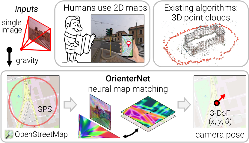
This paper introduces the first approach that can localize single images and image sequences with sub-meter accuracy given the same maps that humans use. These planimetric maps encode only the location and coarse 2D shape of few important objects but not their appearance nor height. Such maps are extremely compact, up to times smaller in size than 3D maps, and can thus be stored on mobile devices and used for on-device localization within large areas. We demonstrate these capabilities with OpenStreetMap (OSM) [46], an openly accessible and community-maintained world map, enabling anyone to localize anywhere for free. This solution does not require building and maintaining costly 3D maps over time nor collecting potentially sensitive mapping data.
Concretely, our algorithm estimates the 3-DoF pose, as position and heading, of a calibrated image in a 2D map. The estimate is probabilistic and can therefore be fused with an inaccurate GPS prior or across multiple views from a multi-camera rig or image sequences. The resulting solution is significantly more accurate than consumer-grade GPS sensors and reaches accuracy levels closer to the traditional pipelines based on feature matching [60, 57].
Our approach, called OrienterNet, is a deep neural network that mimics the way humans orient themselves in their environment when looking at maps, i.e., by matching the metric 2D map with a mental map derived from visual observations [45, 37]. OrienterNet learns to compare visual and semantic data in an end-to-end manner, supervised by camera poses only. This yields accurate pose estimates by leveraging the high diversity of semantic classes exposed by OSM, from roads and buildings to objects like benches and trash cans. OrienterNet is also fast and highly interpretable. We train a single model that generalizes well to previously-unseen cities and across images taken by various cameras from diverse viewpoints – such as car-, bike- or head-mounted, pro or consumer cameras. Key to these capabilities is a new, large-scale training dataset of images crowd-sourced from cities around the world via the Mapillary platform.
Our experiments show that OrienterNet substantially outperforms previous works on localization in driving scenarios and vastly improves its accuracy in AR use cases when applied to data recorded by Aria glasses. We believe that our approach constitutes a significant step towards continuous, large scale, on-device localization for AR and robotics.
| Map type | SfM SLAM | Satellite images | OpenStreetMap (our work) |
| What? | 3D points +features | pixel intensity | polygons, lines, points |
| Explicit geometry? | 3D | ✗ | 2D |
| Visual appearance? | ✓ | ✓ | ✗ |
| Freely available | ✗ | ✗ | ✓ |
| Storage for | |||
| Size reduction vs SfM | - | 550 | 8800 |
2 Related work
We can localize an image in the world using several types of map representations: 3D maps built from ground images, 2D overhead satellite images, or simpler planimetric maps from OpenStreetMap. Table 1 summarizes their differences.
Mapping with ground-level images is the most common approach to date. Place recognition via image retrieval provides a coarse localization given a set of reference images [23, 72, 32, 4]. To estimate centimeter-accurate 6-DoF poses, algorithms based on feature matching require 3D maps [31, 60, 39, 57]. These are composed of sparse point clouds, which are commonly built with Structure-from-Motion (SfM) [67, 22, 2, 61, 43, 36] from sparse points matched across multiple views [38, 9, 53]. The pose of a new query image is estimated by a geometric solver [33, 10, 26] from correspondences with the map. While some works [79, 70] leverage additional sensor inputs, such as a coarse GPS location, gravity direction, and camera height, recent localization systems are highly accurate and robust mostly thanks to learned features [18, 58, 51, 19, 73].
This however involves 3D maps with a large memory footprint as they store dense 3D point clouds with high-dimensional visual descriptors. There is also a high risk of leaking personal data into the map. To mitigate this, some works attempt to compress the maps [13, 39, 12] or use privacy-preserving representations for the scene appearance [20, 44, 81] or geometry [68, 69]. These however either degrade the accuracy significantly or are easily reverted [50].
Localization with overhead imagery reduces the problem to estimating a 3-DoF pose by assuming that the world is mostly planar and that the gravity direction is often given by ubiquitous onboard inertial sensors. A large body of work focuses on cross-view ground-to-satellite localization. While more compact than 3D maps, satellite images are expensive to capture, generally not free, and still heavy to store at high resolution. Most approaches only estimate a coarse position through patch retrieval [30, 63, 65, 82]. In addition, works that estimate an orientation are not accurate [64, 62, 77], yielding errors of over several meters.
Other works rely on sensors that directly provide 3D metric information, such as 2D intensity maps from Lidar [8, 40] or radar [7, 71]. They all perform template matching between 2D map and sensor overhead views, which is both accurate and robust, but require expensive specialized sensors, unsuitable for consumer AR applications. Our work shows how monocular visual priors can substitute such sensors to perform template matching from images only.
Planimetric maps discard any appearance and height information to retain only the 2D location, shape and type of map elements. OSM is a popular platform for such maps as it is free and available globally. Given a query area, its open API exposes a list of geographic features as polygons with metadata, including fine-grained semantic information with over a thousand different object types. Past works however design detectors for a single or few semantic classes, which lacks robustness. These include building outlines [5, 6, 15, 16, 17, 74, 75], road contours [54, 21] or intersections [41, 47, 78], lane markings [25, 48], street furniture [76, 14], or even text [27].
Recent works leverage more cues by computing richer representations from map tiles using end-to-end deep networks [56, 80]. They estimate only a coarse position as they retrieve map tiles with global image descriptors. In indoor scenes, floor plans are common planimetric maps used by existing works [28, 42]. They require height or visibility information that is typically not available for outdoor spaces. Our approach yields a significant step up in accuracy and robustness over all previous works by combining the constraints of projective geometry with the expressivity of end-to-end learning, leveraging all semantic classes available in OSM.
3 Localizing single images in 2D maps
Problem formulation: In a typical localization scenario, we aim to estimate the absolute 6-DoF pose of an image in the world. Under realistic assumptions, we reduce this problem to estimating a 3-DoF pose consisting of a location and heading angle . Here we consider a topocentric coordinate system whose -- axes correspond to the East-North-vertical directions.
First, we can easily assume to know the direction of the gravity, an information that humans naturally possess from their inner ear and that can be estimated by the inertial unit embedded in most devices. We also observe that our world is mostly planar and that the motion of people and objects in outdoor spaces is mostly restricted to 2D surface. The precise height of the camera can always be estimated as the distance to the ground in a local SLAM reconstruction.
Inputs: We consider an image with known pinhole camera calibration. The image is rectified via a homography computed from the known gravity such that its roll and tilt are zero – its principal axis is then horizontal. We are also given a coarse location prior . This can be a noisy GPS position or a previous localization estimate and can be off by over 20 meters. This is a realistic assumption for a consumer-grade sensor in a multi-path environment like a urban canyon.
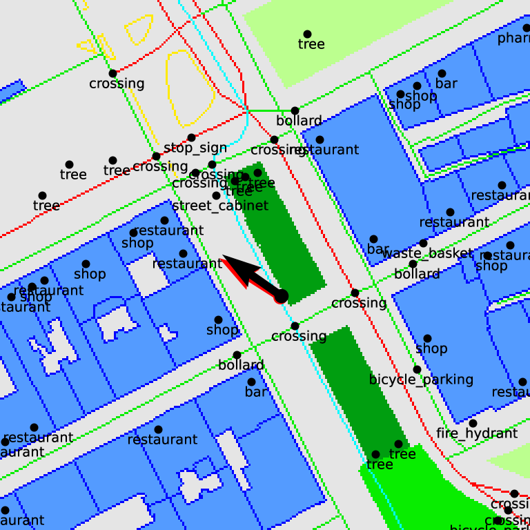
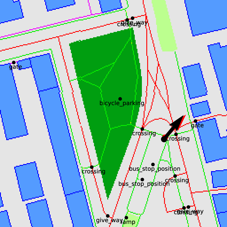
The map data is queried from OSM as a square area centered around and whose size depends on how noisy the prior is. The data consists of a collection of polygons, lines, and points, each of a given semantic class and whose coordinates are given in the same local reference frame.
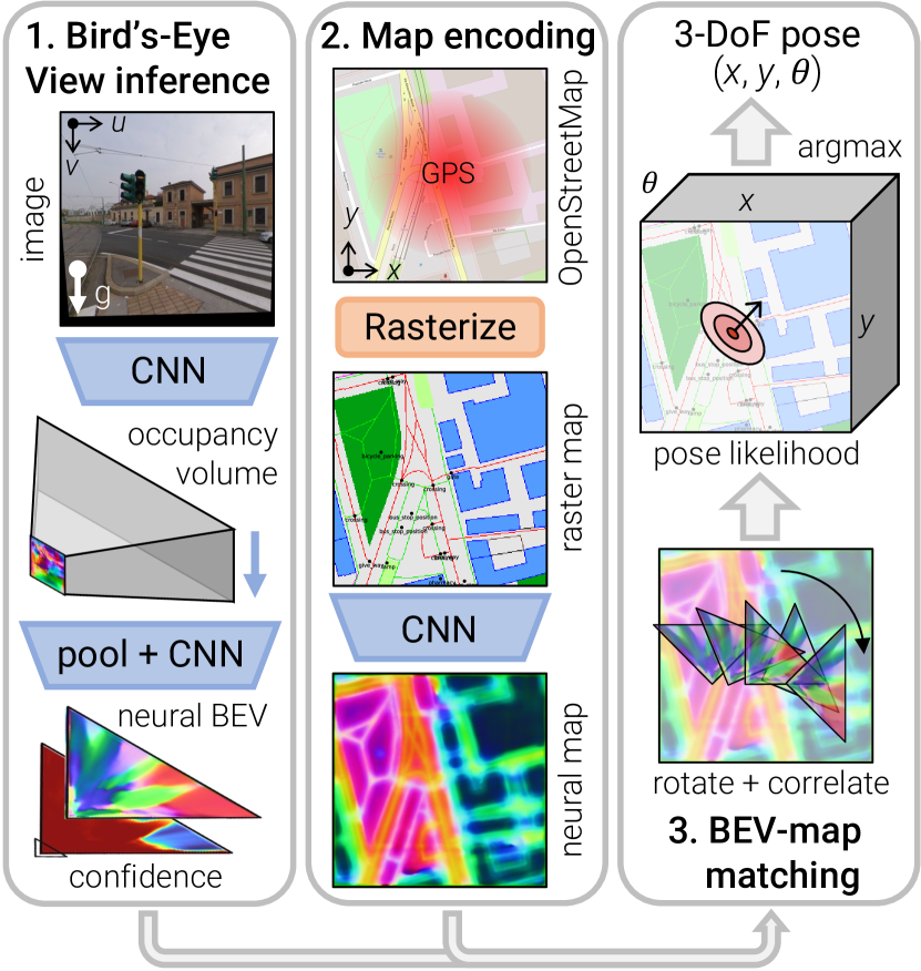
Overview – Figure 2: OrienterNet consists of three modules: 1) The image-CNN extracts semantic features from the image and lifts them to an orthographic Bird’s-Eye View (BEV) representation by inferring the 3D structure of the scene. 2) The OSM map is encoded by the map-CNN into a neural map that embeds semantic and geometric information. 3) We estimate a probability distribution over camera poses by exhaustively matching the BEV against the map.
3.1 Neural Bird’s-Eye View inference
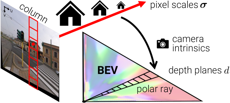
Overview: From a single image , we infer a BEV representation distributed on a grid aligned with the camera frustum and composed of -dimensional features. Each feature on the grid is assigned a confidence, yielding a matrix . This BEV is akin to a mental map that humans infer from their environment when self-localizing in an overhead map [45, 37].
Cross-modal matching between the image and the map requires extracting semantic information from visual cues. It has been shown that monocular depth estimation can rely on semantic cues [3] and that both tasks have a beneficial synergy [29, 34]. We thus rely on monocular inference to lift semantic features to the BEV space. Following past works that tackle semantic tasks [52, 49, 55], we obtain the neural BEV in two steps: i) we transfer image features to a polar representation by mapping image columns to polar rays, and ii) we resample the polar grid into a Cartesian grid (Fig. 3).
Polar representation: A CNN first extracts a feature map from the image. We consider depth planes sampled in front of the camera with a regular interval , i.e. with values . Since the image is gravity-aligned, each of the columns in corresponds to a vertical plane in the 3D space. We thus map each column to a ray in the polar representation . We do so by predicting, for each polar cell , a probability distribution over the pixels in the corresponding image column:
| (1) |
Instead of directly regressing the distribution over depths, we regress a distribution over scales that are independent from the camera calibration parameters. The scale is the ratio of object sizes in the 3D world and in the image [3] and is equal to the ratio of the focal length and depth. We consider a set of log-distributed scales
| (2) |
also predicts, for each pixel , a score vector whose elements correspond to the scale bins . We then obtain the distribution for each depth bin as
| (3) |
where denotes the linear interpolation.
This formulation is equivalent to an attention mechanism from polar rays to image columns with scores resampled from linear depths to log scales. When the scale is ambiguous and difficult to infer, visual features are spread over multiple depths along the ray but still provide geometric constraints for well-localized map points [35]. Works tailored to driving scenarios [52, 49, 55] consider datasets captured by cameras with identical models and directly regress . They therefore encode the focal length in the network weights, learning the mapping from object scale to depth. Differently, our formulation can generalize to arbitrary cameras at test time by assuming that the focal length is an input to the system.
BEV grid: We map the polar features to a Cartesian grid of size via linear interpolation along the lateral direction from polar rays to columns spaced by the same interval . The resulting feature grid is then processed by a small CNN that outputs the neural BEV and confidence .
3.2 Neural map encoding
We encode the planimetric map into a neural map that combines geometry and semantics.
Map data: OpenStreetMap elements are defined, depending on their semantic class, as polygonal areas, multi-segment lines, or single points. Examples of areas include building footprints, grass patches, parking lots; lines include road or sidewalk center lines, building outlines; points include trees, bus stops, shops, etc. Appendix B.1 lists all classes. The accurate positioning of these elements provides geometric constraints necessary for localization, while their rich semantic diversity helps disambiguate different poses.
Preprocessing: We first rasterize the areas, lines, and points as a 3-channels image with a fixed ground sampling distance , e.g. . This representation is more informative and accurate than the naive rasterization of human-readable OSM tiles performed in previous works [56, 80].
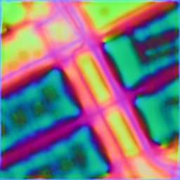
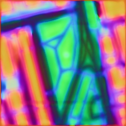
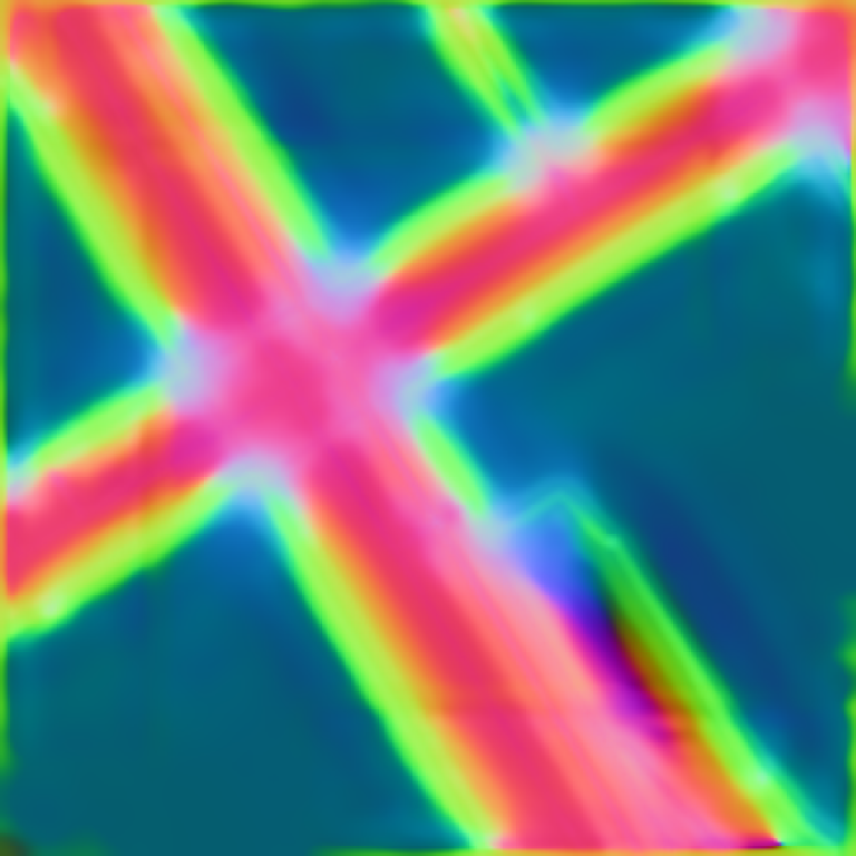
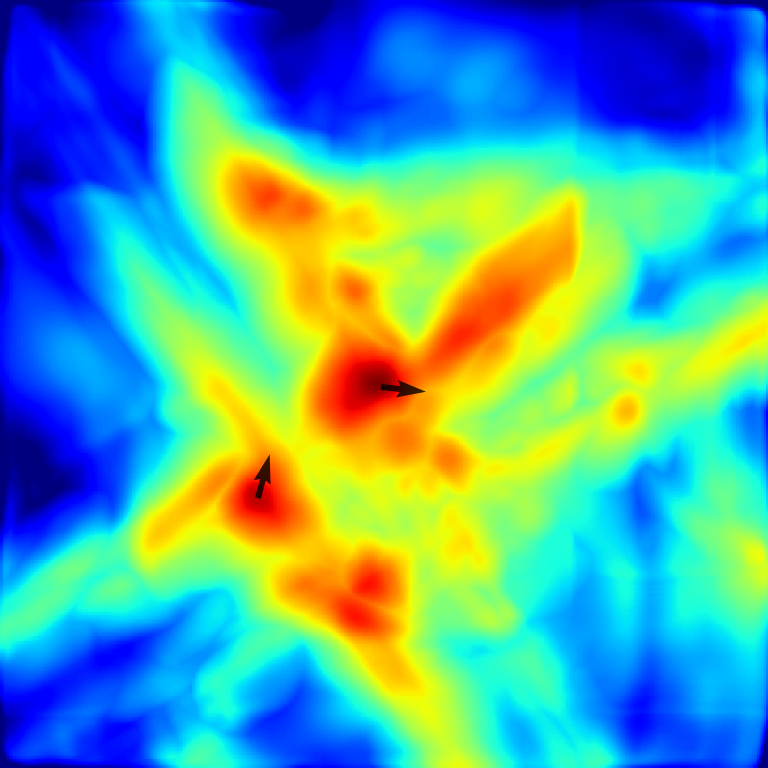
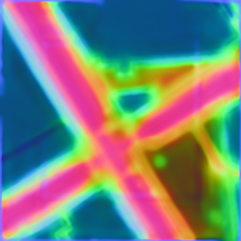
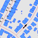
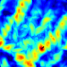
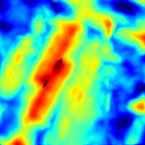
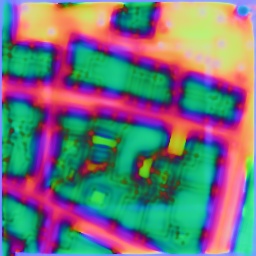
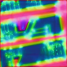
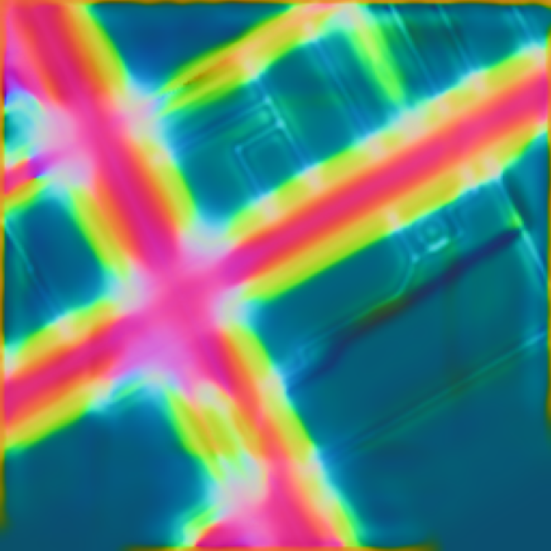
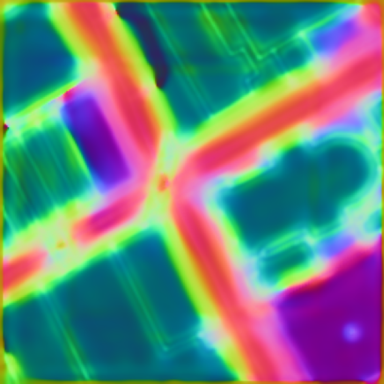
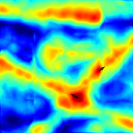
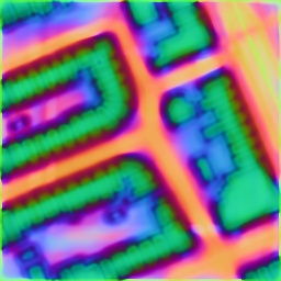
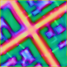
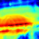
Encoding: We associate each class with an -dimensional embedding that is learned, yielding a feature map. It is then encoded into the neural map by a CNN , which extracts geometric features useful for localization. is not normalized as we let modulate its norm as importance weight in the matching. Examples in Fig. 4 reveal that often looks like a distance field where we can clearly recognize distinctive features like corners or adjoining boundaries of buildings.
also predicts a unary location prior for each cell of the map. This score reflects how likely an image is to be taken at each location. We rarely expect images to be taken in, for example, rivers or buildings.
gravity-aligned image
input map
likelihood
log-likelihood
neural map
Hand-held (MGL)
width 1pt
 \begin{overpic}[width=401.09981pt]{figures/qualitative_camera-ready_main/nantes_A3N3NjithyGDFa3o8eZNDg_front_likelihood.pdf}
\put(5.0,5.0){\color[rgb]{0,0,0}\definecolor[named]{pgfstrokecolor}{rgb}{0,0,0}\pgfsys@color@gray@stroke{0}\pgfsys@color@gray@fill{0}\scriptsize$\Delta\bm{\mathrm{\xi}}{=}0.4\text{m}/2.5\degree$}
\end{overpic}

 \begin{overpic}[width=401.09981pt]{figures/qualitative_camera-ready_main/milan_pbXc2AMJO9iYS1PXxu0MFT_right_likelihood.pdf}\put(5.0,5.0){\color[rgb]{0,0,0}\definecolor[named]{pgfstrokecolor}{rgb}{0,0,0}\pgfsys@color@gray@stroke{0}\pgfsys@color@gray@fill{0}\scriptsize$\Delta\bm{\mathrm{\xi}}{=}1.1\text{m}/3.5\degree$}
\end{overpic}
Head-mounted (Aria)
width 1pt
 \begin{overpic}[width=401.09981pt]{figures/qualitative_camera-ready_main/reloc_seattle_downtown_208273094103158__208273094103158_RGB__000516919739000__000034_likelihood.pdf}\put(5.0,5.0){\color[rgb]{0,0,0}\definecolor[named]{pgfstrokecolor}{rgb}{0,0,0}\pgfsys@color@gray@stroke{0}\pgfsys@color@gray@fill{0}\scriptsize$\Delta\bm{\mathrm{\xi}}{=}0.4\text{m}/5.7\degree$}
\put(5.0,15.0){\color[rgb]{0,0,0}\definecolor[named]{pgfstrokecolor}{rgb}{0,0,0}\pgfsys@color@gray@stroke{0}\pgfsys@color@gray@fill{0}\scriptsize$\Delta\text{GPS}{=}30.9\text{m}$}
\end{overpic}
 \begin{overpic}[width=401.09981pt]{figures/qualitative_camera-ready_main/reloc_seattle_westlake_383662566932182__383662566932182_RGB__000835539815000__000341_likelihood.pdf}\put(5.0,5.0){\color[rgb]{0,0,0}\definecolor[named]{pgfstrokecolor}{rgb}{0,0,0}\pgfsys@color@gray@stroke{0}\pgfsys@color@gray@fill{0}\scriptsize$\Delta\bm{\mathrm{\xi}}{=}1.0\text{m}/2.2\degree$}
\put(5.0,15.0){\color[rgb]{0,0,0}\definecolor[named]{pgfstrokecolor}{rgb}{0,0,0}\pgfsys@color@gray@stroke{0}\pgfsys@color@gray@fill{0}\scriptsize$\Delta\text{GPS}{=}13.9\text{m}$}
\end{overpic}
Car-mounted (KITTI)
width 1pt
\begin{overpic}[width=193.77362pt]{figures/qualitative_camera-ready_main/kitti_2011_09_30_2011_09_30_drive_0020_sync_image_02_data_0000001026.png_image.jpg}\put(5.0,2.0){\color[rgb]{1,1,1}\definecolor[named]{pgfstrokecolor}{rgb}{1,1,1}\pgfsys@color@gray@stroke{1}\pgfsys@color@gray@fill{1}\scriptsize$\Delta\bm{\mathrm{\xi}}{=}0.7\text{m}/1.7\degree\quad{\Delta\text{lateral}}{=}0.6\text{m}\quad{\Delta\text{long.}}{=}0.3\text{m}$}
\end{overpic}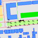
 \begin{overpic}[width=193.77362pt]{figures/qualitative_camera-ready_main/kitti_2011_10_03_2011_10_03_drive_0027_sync_image_02_data_0000000256.png_image.jpg}\put(5.0,2.0){\color[rgb]{1,1,1}\definecolor[named]{pgfstrokecolor}{rgb}{1,1,1}\pgfsys@color@gray@stroke{1}\pgfsys@color@gray@fill{1}\scriptsize$\Delta\bm{\mathrm{\xi}}{=}1.0\text{m}/0.7\degree\quad{\Delta\text{lateral}}{=}0.2\text{m}\quad{\Delta\text{long.}}{=}1.0\text{m}$}
\end{overpic}
 \begin{overpic}[width=193.77362pt]{figures/qualitative_camera-ready_main/kitti_2011_10_03_2011_10_03_drive_0027_sync_image_02_data_0000003621.png_image.jpg}\put(5.0,2.0){\color[rgb]{1,1,1}\definecolor[named]{pgfstrokecolor}{rgb}{1,1,1}\pgfsys@color@gray@stroke{1}\pgfsys@color@gray@fill{1}\scriptsize$\Delta\bm{\mathrm{\xi}}{=}0.6\text{m}/2.0\degree\quad{\Delta\text{lateral}}{=}0.5\text{m}\quad{\Delta\text{long.}}{=}0.3\text{m}$}
\end{overpic}
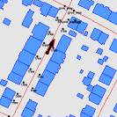
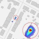

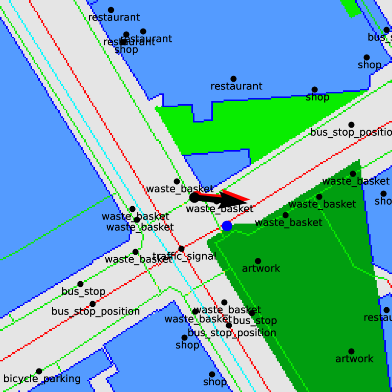
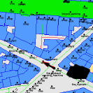
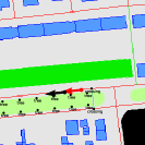
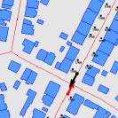
Map legend: building area and outline, road, footway, cycleway, grass, park, playground, parking, fence
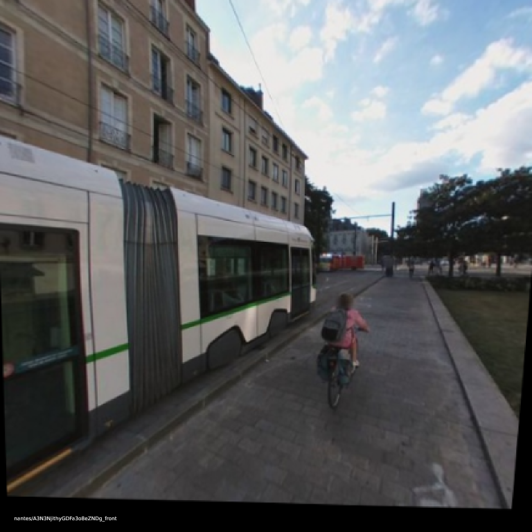
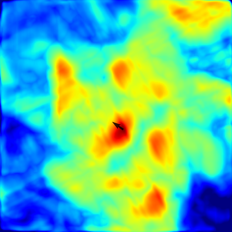
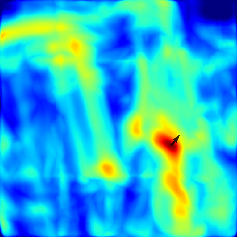
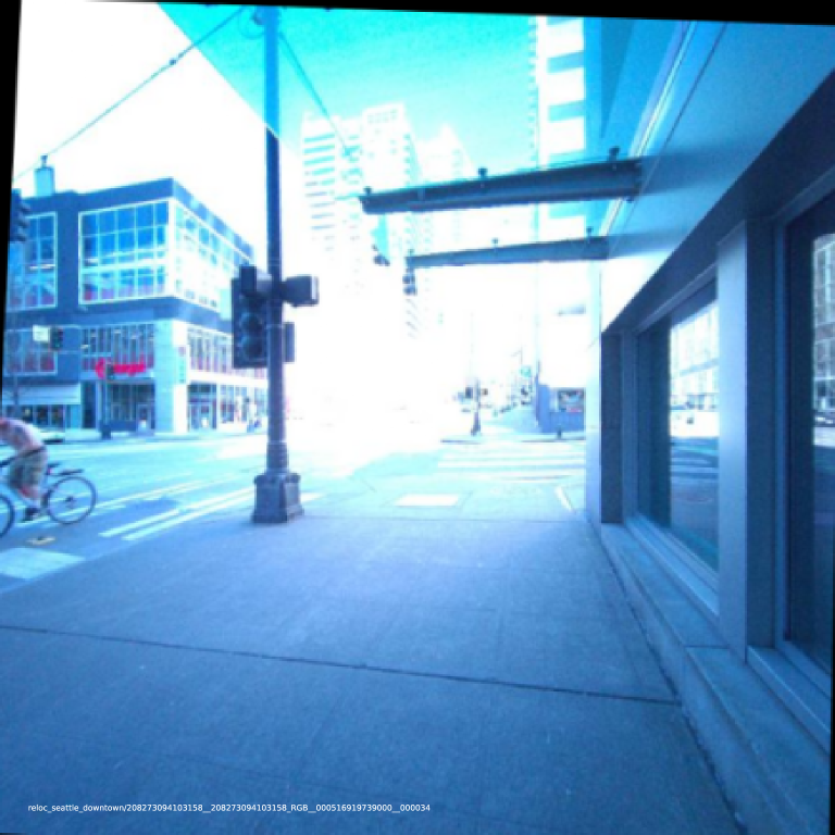
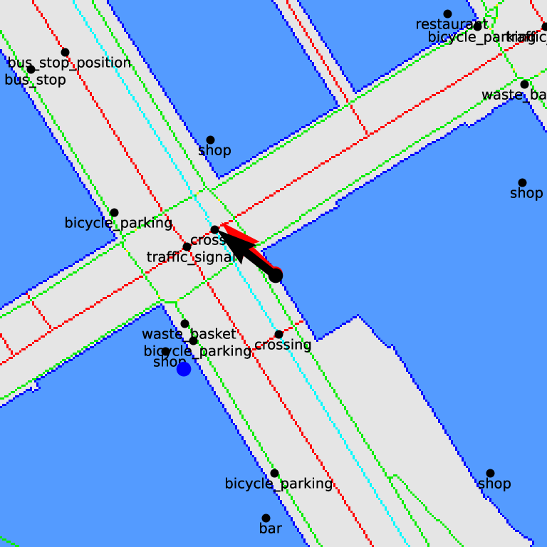
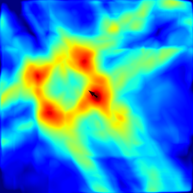
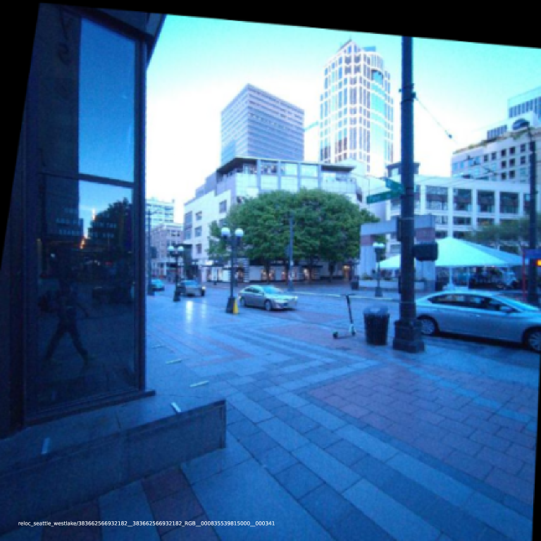
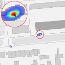
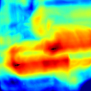
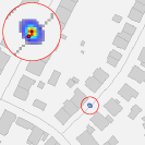
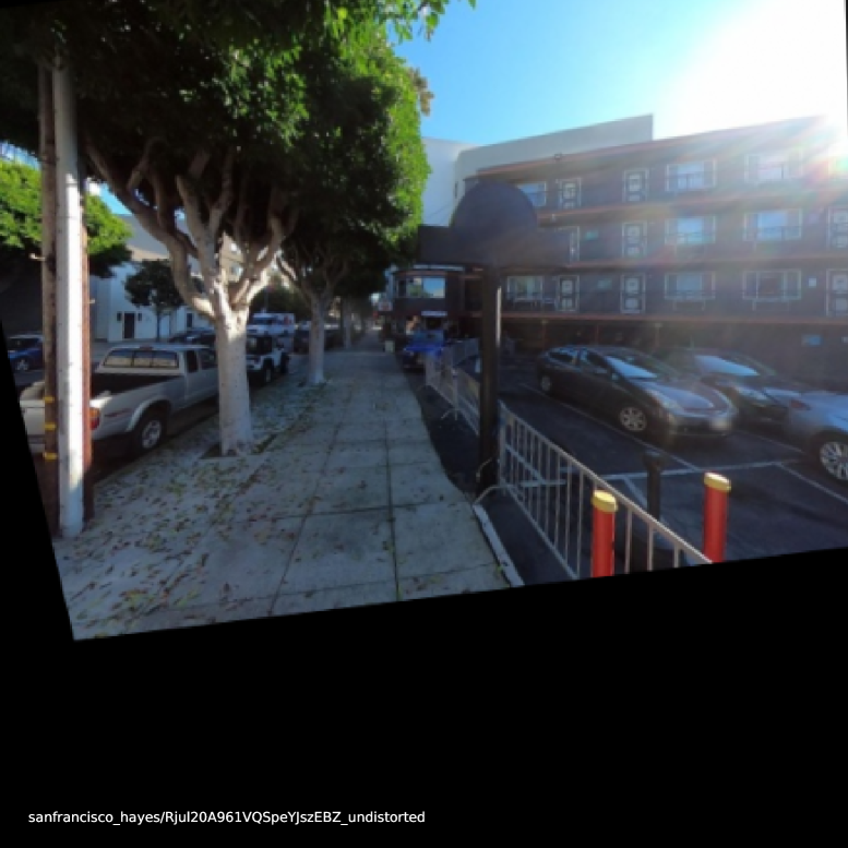
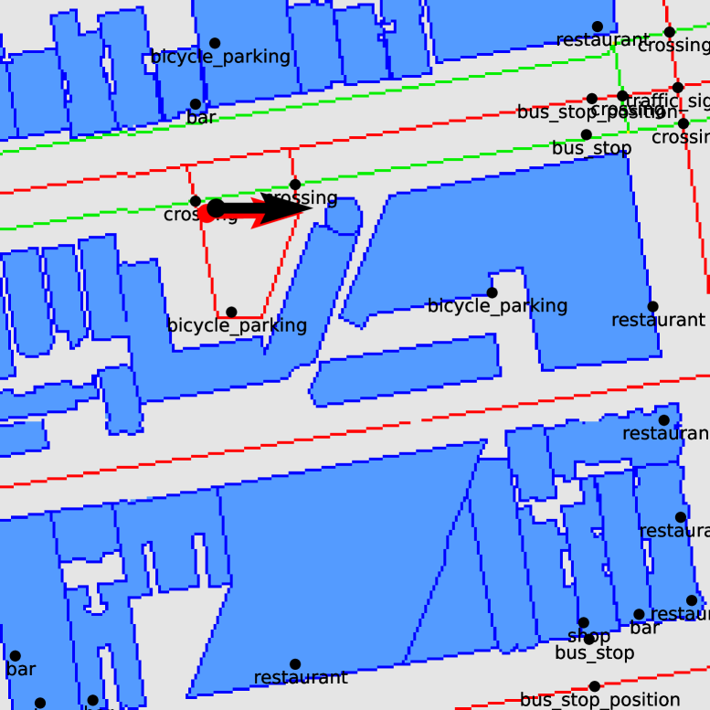
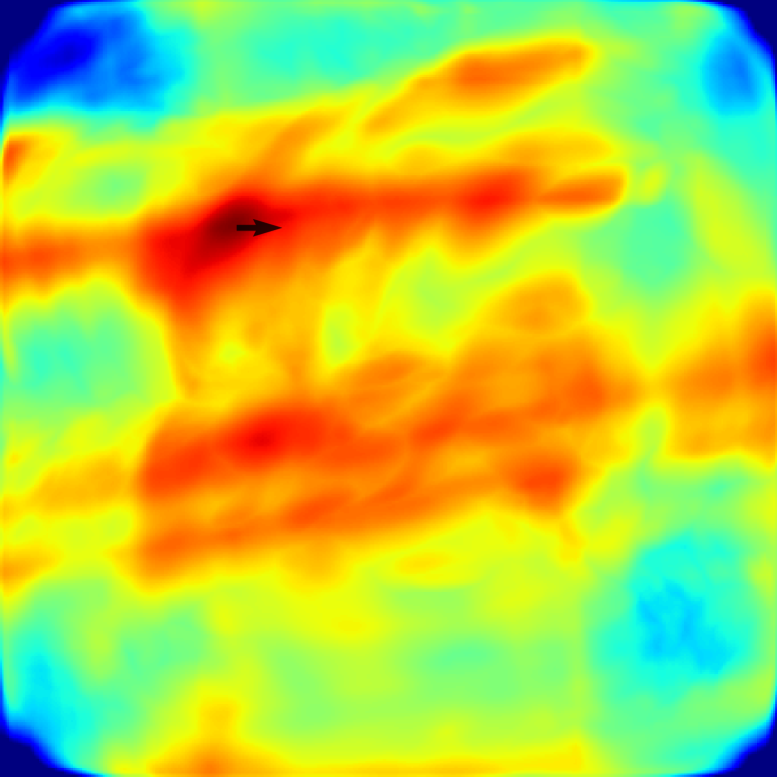
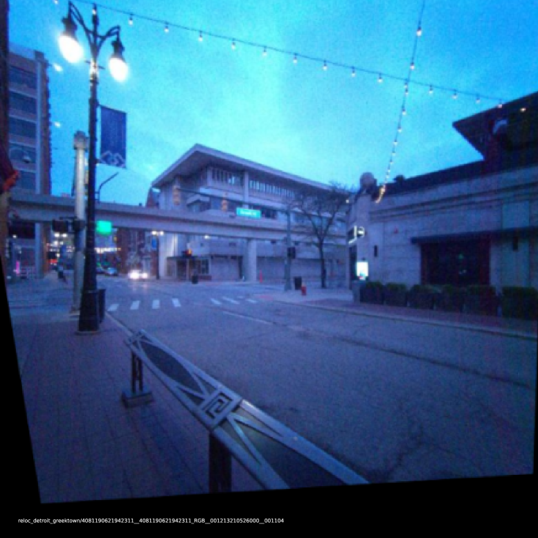
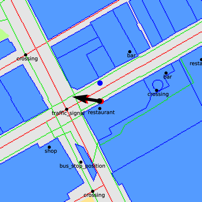
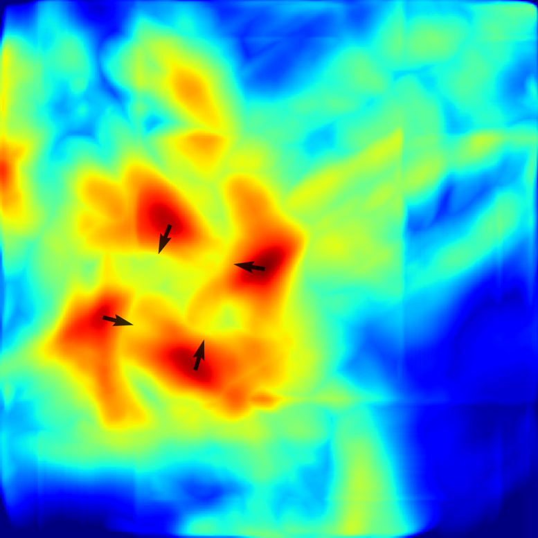
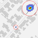
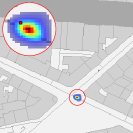
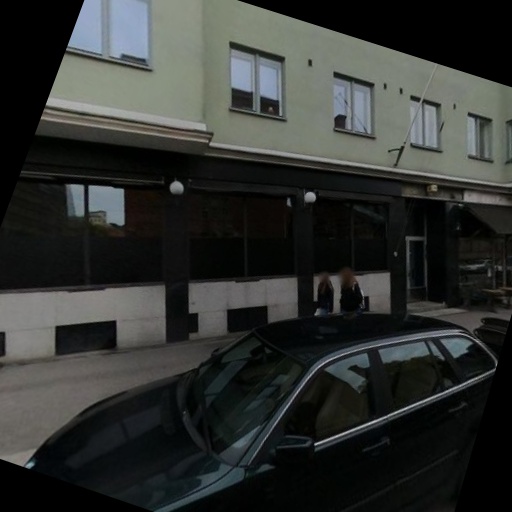
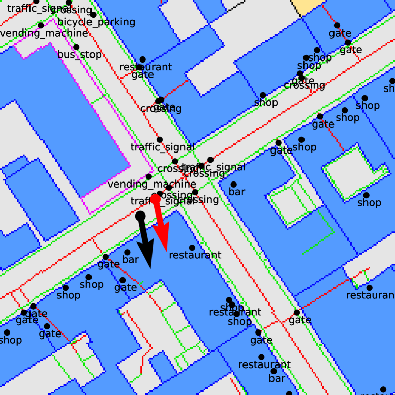
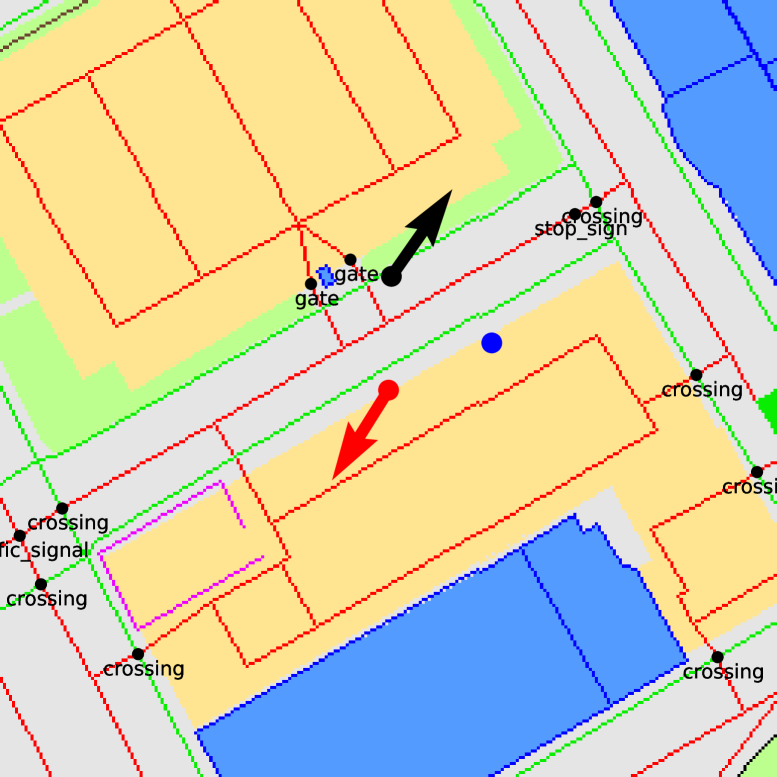
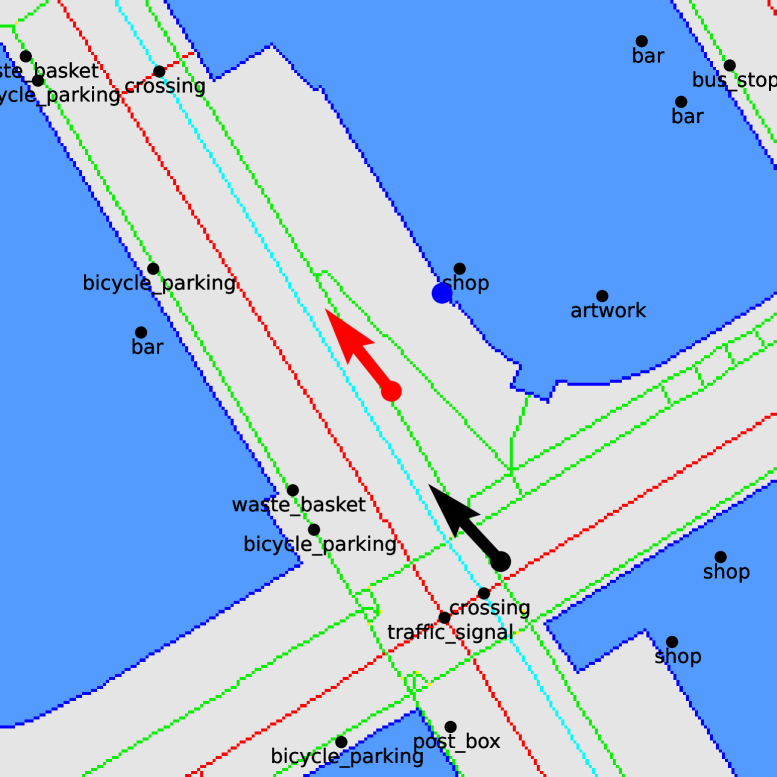
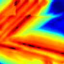
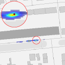
 ) are close to the ground truth (red arrow) and more accurate than the noisy GPS (blue dot ).
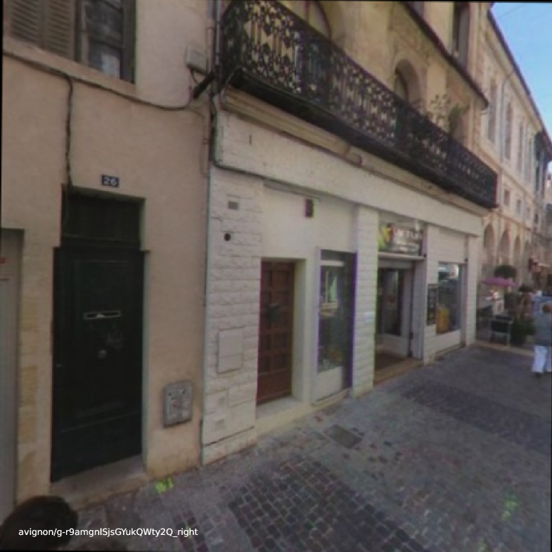
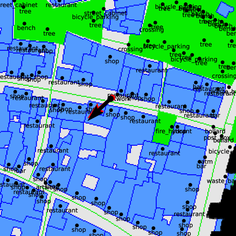
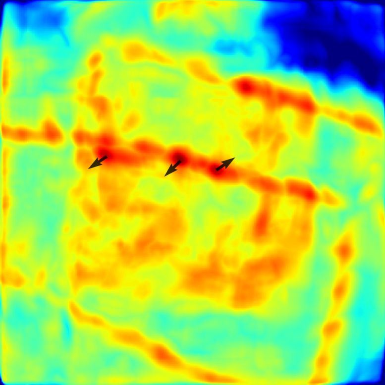
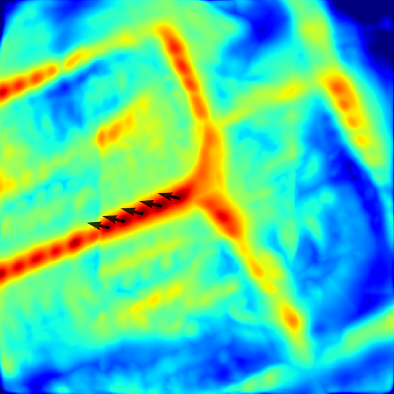
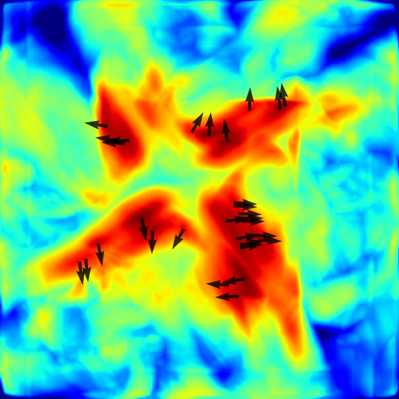
The model effectively leverages building corners and boundaries, crosswalks, sidewalks, road intersections, trees, and other common urban objects.
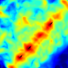
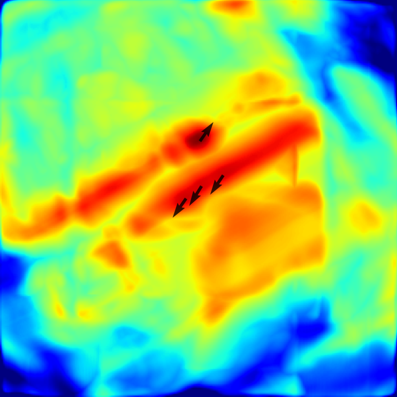
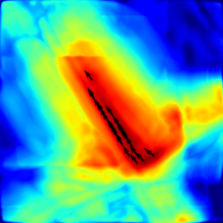
Likelihood maps can be multi-modal in scenes with repeated elements (last two rows) - we show the predicted orientations at local maxima as small arrows.
3.3 Pose estimation by template matching
Probability volume: We estimate a discrete probability distribution over camera poses . This is interpretable and fully captures the uncertainty of the estimation. As such, the distribution is multimodal in ambiguous scenarios. Figure 4 shows various examples. This makes it easy to fuse the pose estimate with additional sensors like GPS. Computing this volume is tractable because the pose space has been reduced to 3 dimensions. It is discretized into each map location and rotations sampled at regular intervals.
This yields a probability volume such that . It is the combination of an image-map matching term and the location prior :
| (4) |
and represent image-conditioned and image-independent un-normalized log scores. is broadcasted along the rotation dimension and softmax normalizes the probability distribution.
Image-map matching: Exhaustively matching the neural map and the BEV yields a score volume . Each element is computed by correlating with transformed by the corresponding pose as
| (5) |
where transforms a 2D point from BEV to map coordinate frame. The confidence masks the correlation to ignore some parts of the BEV space, such as occluded areas. This formulation benefits from an efficient implementation by rotating times and performing a single convolution as a batched multiplication in the Fourier domain [8, 7].
Pose inference: We estimate a single pose by maximum likelihood: . When the distribution is mostly unimodal, we can obtain a measure of uncertainty as the covariance of around [7].
4 Sequence and multi-camera localization
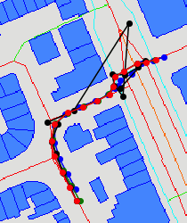
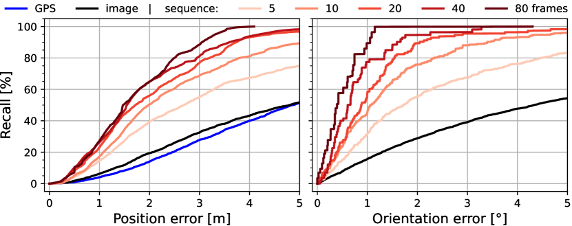
Single-image localization is ambiguous in locations that exhibit few distinctive semantic elements or repeated patterns. Such challenge can be disambiguated by accumulating additional cues over multiple views when their relative poses are known. These views can be either sequences of images with poses from VI SLAM or simultaneous views from a calibrated multi-camera rig. Figure 5 shows an example of such difficult scenario disambiguated by accumulating predictions over time. Different frames constrain the pose in different directions, e.g. before and after an intersection. Fusing longer sequences yields a higher accuracy (Fig. 6).
Let us denote the unknown absolute pose of view and the known relative pose from view to . For an arbitrary reference view , we express the joint likelihood over all single-view predictions as
| (6) |
where denotes the pose composition operator. This is efficiently computed by warping each probability volume to the reference frame . We can also localize each image of a continuous stream via iterative warping and normalization, like in the classical Markov localization [66, 11].
gravity-aligned image
single-frame
sequence
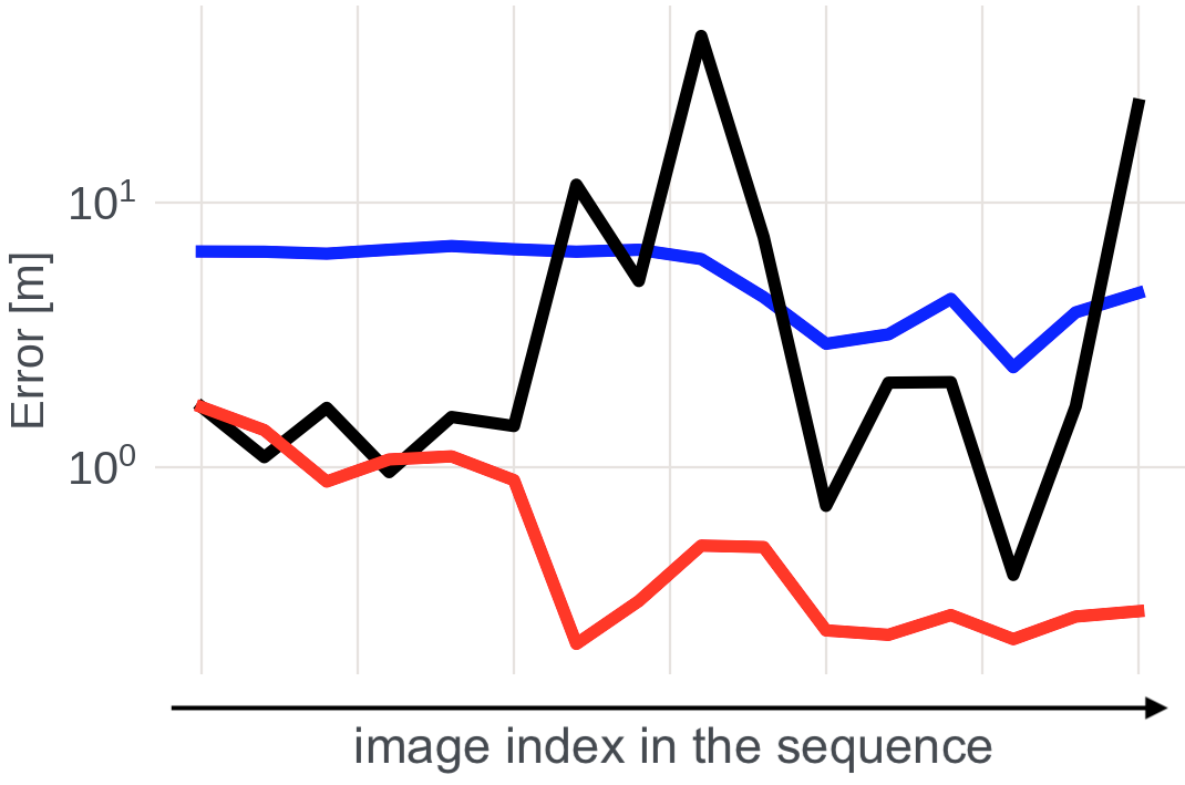
GPS single-frame sequence GT
5 Training a single strong model
Supervision: OrienterNet is trained in a supervised manner from pairs of single images and ground truth (GT) poses. The architecture is differentiable and all components are trained simultaneously by back-propagation. We simply maximize the log-likelihood of the ground truth pose : . The tri-linear interpolation of provides sub-pixel supervision.
| Model architecture | Position R@Xm | Orientation R@X° | ||||
| 1m | 3m | 5m | 1° | 3° | 5° | |
| Retrieval (a) | 2.02 | 15.21 | 24.21 | 4.50 | 18.61 | 32.48 |
| Refinement (b) | 8.09 | 26.02 | 35.31 | 14.92 | 36.87 | 45.19 |
| OrienterNet - planar (c) | 14.28 | 44.59 | 56.08 | 20.43 | 50.34 | 64.30 |
| OrienterNet - full | 15.78 | 47.75 | 58.98 | 22.14 | 52.56 | 66.32 |
Training dataset: We train a single model that generalizes to unseen locations with arbitrary kinds of images. We collect images from the Mapillary platform, which exposes the camera calibration, noisy GPS measurement, and the 6-DoF pose in a global reference frame, obtained with a fusion of SfM and GPS. The resulting Mapillary Geo-Localization (MGL) dataset includes 760k images from 12 cities in Europe and the US, captured by cameras that are handheld or mounted on cars or bikes, with GT poses and OSM data. Models trained on MGL generalize well to other datasets thanks to the diversity of cameras, locations, motions, and maps. All images are publicly available under a CC-BY-SA license via the Mapillary API. We believe that this dataset will significantly facilitate research on visual geo-localization.
| Map | Approach | Training dataset | Lateral R@Xm | Longitudinal R@Xm | Orientation R@X° | ||||||
| 1m | 3m | 5m | 1m | 3m | 5m | 1° | 3° | 5° | |||
| Satellite | DSM [64] | KITTI | 10.77 | 31.37 | 48.24 | 3.87 | 11.73 | 19.50 | 3.53 | 14.09 | 23.95 |
| VIGOR [82] | KITTI | 17.38 | 48.20 | 70.79 | 4.07 | 12.52 | 20.14 | - | - | - | |
| refinement [62] | KITTI | 27.82 | 59.79 | 72.89 | 5.75 | 16.36 | 26.48 | 18.42 | 49.72 | 71.00 | |
| OpenStreetMap | retrieval [77, 56] | MGL | 37.47 | 66.24 | 72.89 | 5.94 | 16.88 | 26.97 | 2.97 | 12.32 | 23.27 |
| refinement [62] | MGL | 50.83 | 78.10 | 82.22 | 17.75 | 40.32 | 52.40 | 31.03 | 66.76 | 76.07 | |
| OrienterNet (a) | MGL | 53.51 | 88.85 | 94.47 | 26.25 | 59.84 | 70.76 | 34.26 | 73.51 | 89.45 | |
| + sequence (b) | MGL | 79.71 | 97.44 | 98.67 | 55.21 | 95.27 | 99.51 | 77.87 | 97.76 | 100. | |
| OrienterNet (c) | KITTI | 51.26 | 84.77 | 91.81 | 22.39 | 46.79 | 57.81 | 20.41 | 52.24 | 73.53 | |
| OrienterNet (d) | MGL+KITTI | 65.91 | 92.76 | 96.54 | 33.07 | 65.18 | 75.15 | 35.72 | 77.49 | 91.51 | |
Implementation: and are U-Nets with ResNet-101 and VGG-16 encoders. has 4 residual blocks. We use scale bins, rotations. The BEV has size with resolution . For training, we render maps centered around points randomly sampled within of the GT pose. Localizing in such map takes on an NVIDIA RTX 2080 GPU, with for the BEV inference and for the matching.
6 Experiments
We evaluate our single model for localization in the context of both driving and AR. Figure 4 shows qualitative examples, while Fig. 5 illustrates the effectiveness of multi-frame fusion. Our experiments show that: 1) OrienterNet is more effective than existing deep networks for localization with 2D maps; 2) Planimetric maps help localize more accurately than overhead satellite imagery; 3) OrienterNet is significantly more accurate than an embedded consumer-grade GPS sensor when considering multiple views.
6.1 Validating design decisions
Setup: We evaluate the design of OrienterNet on the validation split of our MGL dataset. This ensures an identical distribution of cameras, motions, viewing conditions, and visual features as the training set. We report recall of positions and rotation errors at the three thresholds 1/3/5m and 1/3/5.
Comparing model architectures: We compare OrienterNet to alternative architectures trained on the same dataset: a) Map retrieval [77] replaces the BEV inference and matching by a correlation of the neural map and with a global image embedding. We predict a rotation by considering 4 different neural maps for the N-S-E-W directions. This formulation also regresses a probability volume and is trained identically to OrienterNet. It mimics the retrieval of densely-sampled map patches [56] but is significantly more efficient and practical. b) Featuremetric refinement [62, 59] updates an initial pose by warping a satellite view to the image assuming that the scene is planar, at a fixed height, and gravity-aligned. We replace the satellite view by an OSM map tile. This formulation requires an initial orientation (during both training and testing), which we sample within 45 of the ground truth. c) OrienterNet (planar) replaces the occupancy by warping the image features with a homography as in [62].
Analysis – Table 2: OrienterNet is significantly more accurate than all baselines at all position and rotation thresholds. a) Map retrieval disregards any knowledge of projective geometry and performs mere recognition without any geometric constraint. b) Featuremetric refinement converges to incorrect locations when the initial pose is inaccurate. c) Inferring the 3D geometry of the scene is more effective than assuming that it is planar. This justifies our design decisions.
Model interpretability: We visualize in Fig. 7 multiple internal quantities that help us understand the predictions.
6.2 Application: autonomous driving
Dataset: We consider the localization in driving scenarios with the KITTI dataset [24], following the closest existing setup [62]. To evaluate the zero-shot performance, we use their Test2 split, which does not overlap with the KITTI and MGL training sets. Images are captured by cameras mounted on a car driving in urban and residential areas and have GT poses from RTK. We augment the dataset with OSM maps.
Setup: We compute the position error along directions perpendicular (lateral) and parallel (longitudinal) to the viewing axis [62] since the pose is generally less constrained along the road. We report the recall at 1/3/5m and 1/3/5. The original setup [62] assumes an accurate initial pose randomly sampled within 20m and 10 of the GT. OrienterNet does not require such initialization but only a coarse position-only prior. For fair comparisons, we nevertheless restrict the pose space to the same interval centered around the initial pose. We render map tiles and resize the images such that their focal length matches the median of MGL.
Baselines: We report approaches based on satellite maps and trained by [62] on KITTI. VIGOR [82] and DSM [64] both perform patch retrieval with global descriptors but respectively estimate an additional position offset or the orientation. We also evaluate the featuremetric refinement [62, 59] and baselines based on OSM maps, described in Sec. 6.1. As each scene is visited by a single trajectory, we cannot evaluate approaches based on 3D maps and image matching.
Results: Table 3 (a-b) shows that OrienterNet outperforms all existing approaches based on both satellite and OSM maps, in all metrics. OrienterNet exhibits remarkable zero-shot capabilities as it outperforms approaches trained on KITTI itself. The evaluation also demonstrates that planimetric maps yield better localization, as retrieval and refinement approaches based on them outperform those based on satellite images. The recall at 3m/3°is saturated to over 95% by fusing the predictions from sequences of only 20 seconds.
Generalization: Table 3 (c-d) shows that training OrienterNet solely on KITTI results in overfitting, as the dataset is too small to learn rich semantic representations. Our larger MGL dataset alleviates this issue and enables cross-modal learning with rich semantic classes. Pre-training on MGL and fine-tuning on KITTI yields the best performance.
| City | Setup | Approach | Position R@Xm | Orientation R@X° | ||||
| 1m | 3m | 5m | 1° | 3° | 5° | |||
| Seattle | single | GPS | 1.25 | 8.82 | 18.44 | - | - | - |
| retrieval [77, 56] | 0.88 | 3.81 | 5.95 | 2.83 | 8.36 | 12.96 | ||
| OrienterNet | 3.39 | 14.49 | 23.92 | 6.83 | 20.39 | 30.89 | ||
| multi | GPS | 1.76 | 9.2 | 20.48 | 4.18 | 11.01 | 23.36 | |
| OrienterNet | 21.88 | 61.26 | 72.92 | 33.86 | 72.41 | 83.93 | ||
| Detroit | single | GPS | 3.96 | 27.75 | 51.33 | - | - | - |
| retrieval [77, 56] | 3.31 | 19.83 | 36.76 | 6.48 | 18.40 | 28.88 | ||
| OrienterNet | 6.26 | 32.41 | 51.76 | 15.53 | 39.06 | 54.41 | ||
| multi | GPS | 4.09 | 31.36 | 53.41 | 13.48 | 37.84 | 55.24 | |
| OrienterNet | 17.18 | 68.77 | 89.26 | 44.85 | 88.04 | 96.04 | ||
6.3 Application: augmented reality
We now consider the localization of head-mounted devices for augmented reality (AR). We show that OrienterNet is more accurate than a typical embedded GPS sensor.
Dataset: There is no public benchmark that provides geo-aligned GT poses for images captured with AR devices in diverse outdoor spaces. We thus record our own dataset with Aria [1] glasses. It exhibits patterns typical of AR with noisy consumer-grade sensors and pedestrian viewpoints and motions. We include two locations: i) downtown Seattle, with high-rise buildings, and ii) Detroit, with city parks and lower buildings. We record several image sequences per city, all roughly following the same loop around multiple blocks. We record calibrated RGB images and GPS measurements for each and obtain relative poses and gravity direction from an offline proprietary VI SLAM system. We obtain pseudo-GT global poses by jointly optimizing all sequences based on GPS, VI constraints, and predictions of OrienterNet.
Single-frame localization – Table 4: OrienterNet is consistently more accurate than the GPS, which is extremely noisy in urban canyons like Seattle because of multi-path effects. The performance is however significantly lower than with driving data (Sec. 6.2), which highlights the difficulty of AR-like conditions and the need for further research.
Multi-frame: We now fuse multiple GPS signals or predictions of OrienterNet over the same temporal interval of 10 consecutive keyframes, using imperfect relative poses from VI SLAM. The fusion more than doubles the accuracy of OrienterNet but marginally benefits the GPS sensor because of its high, biased noise, especially in Seattle.
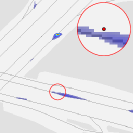
Limitations: Localizing an image or a sequence is challenging when the environments lacks distinctive elements or when they are not registered in the map. OSM may also be spatially inaccurate. Appendix A shows some failure cases.
Map
Image
Depth
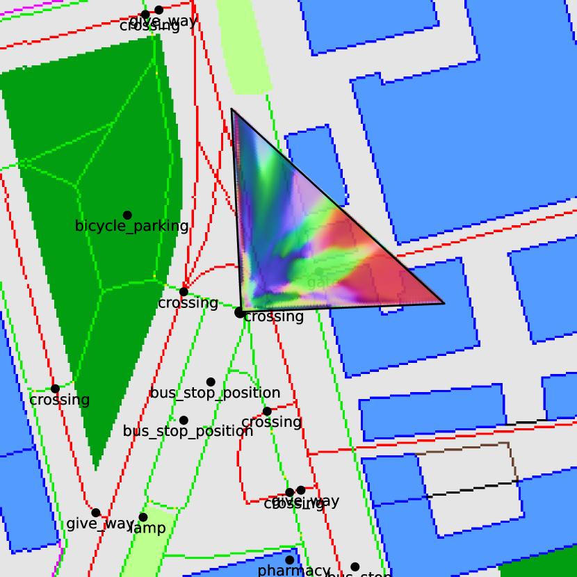
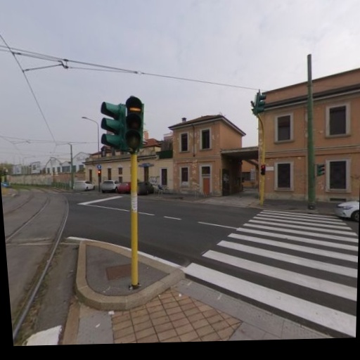
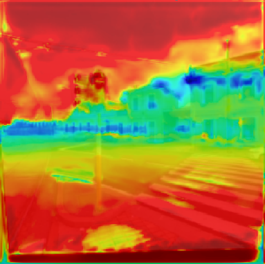

distant close
Neural BEV
BEV confidence


7 Conclusion
OrienterNet is the first deep neural network that can localize an image with sub-meter accuracy within the same 2D planimetric maps that humans use. OrienterNet mimics the way humans orient themselves in their environment by matching the input map with a mental map derived from visual observations. Compared to large and expensive 3D maps that machines have so far relied on, such 2D maps are extremely compact and thus finally enable on-device localization within large environments. OrienterNet is based on globally and freely available maps from OpenStreetMap and can be used by anyone to localize anywhere in the world.
We contribute a large, crowd-sourced training dataset that helps the model generalize well across both driving and AR datasets. OrienterNet significantly improves over existing approaches for 3-DoF localization, pushing the state of the art by a large margin. This opens up exciting prospects for deploying power-efficient robots and AR devices that know where they are without costly cloud infrastructures.
gravity-aligned image
input map
likelihood
log-likelihood
neural map
Hand-held (MGL)
width 1pt
 \begin{overpic}[width=405.43362pt]{figures/qualitative_camera-ready_supp/avignon_g-r9amgnlSjsGYukQWty2Q_right_likelihood.pdf}
\put(5.0,5.0){\color[rgb]{0,0,0}\definecolor[named]{pgfstrokecolor}{rgb}{0,0,0}\pgfsys@color@gray@stroke{0}\pgfsys@color@gray@fill{0}\scriptsize$\Delta\bm{\mathrm{\xi}}{=}0.9\text{m}/4.3\degree$}
\end{overpic}
 \begin{overpic}[width=405.43362pt]{figures/qualitative_camera-ready_supp/sanfrancisco_hayes_Rjul20A961VQSpeYJszEBZ_undistorted_likelihood.pdf}\put(5.0,5.0){\color[rgb]{0,0,0}\definecolor[named]{pgfstrokecolor}{rgb}{0,0,0}\pgfsys@color@gray@stroke{0}\pgfsys@color@gray@fill{0}\scriptsize$\Delta\bm{\mathrm{\xi}}{=}1.9\text{m}/0.4\degree$}
\end{overpic}
Head-mounted (Aria)
width 1pt
 \begin{overpic}[width=405.43362pt]{figures/qualitative_camera-ready_supp/reloc_detroit_greektown_4081190621942311__4081190621942311_RGB__001213210526000__001104_likelihood.pdf}\put(5.0,5.0){\color[rgb]{0,0,0}\definecolor[named]{pgfstrokecolor}{rgb}{0,0,0}\pgfsys@color@gray@stroke{0}\pgfsys@color@gray@fill{0}\scriptsize$\Delta\bm{\mathrm{\xi}}{=}1.2\text{m}/0.2\degree$}
\put(5.0,15.0){\color[rgb]{0,0,0}\definecolor[named]{pgfstrokecolor}{rgb}{0,0,0}\pgfsys@color@gray@stroke{0}\pgfsys@color@gray@fill{0}\scriptsize$\Delta\text{GPS}{=}11.6\text{m}$}
\end{overpic}
 \begin{overpic}[width=405.43362pt]{figures/qualitative_camera-ready_supp/reloc_detroit_greektown_4081190621942311__4081190621942311_RGB__001088211335000__000979_likelihood.pdf}\put(5.0,5.0){\color[rgb]{0,0,0}\definecolor[named]{pgfstrokecolor}{rgb}{0,0,0}\pgfsys@color@gray@stroke{0}\pgfsys@color@gray@fill{0}\scriptsize$\Delta\bm{\mathrm{\xi}}{=}2.1\text{m}/2.3\degree$}
\put(5.0,15.0){\color[rgb]{0,0,0}\definecolor[named]{pgfstrokecolor}{rgb}{0,0,0}\pgfsys@color@gray@stroke{0}\pgfsys@color@gray@fill{0}\scriptsize$\Delta\text{GPS}{=}3.7\text{m}$}
\end{overpic}
Car-mounted (KITTI)
width 1pt
\begin{overpic}[width=193.77362pt]{figures/qualitative_camera-ready_supp/kitti_2011_09_26_2011_09_26_drive_0039_sync_image_02_data_0000000120.png_image.jpg}\put(5.0,2.0){\color[rgb]{1,1,1}\definecolor[named]{pgfstrokecolor}{rgb}{1,1,1}\pgfsys@color@gray@stroke{1}\pgfsys@color@gray@fill{1}\scriptsize$\Delta\bm{\mathrm{\xi}}{=}0.9\text{m}/1.7\degree\quad{\Delta\text{lateral}}{=}0.3\text{m}\quad{\Delta\text{long.}}{=}0.9\text{m}$}
\end{overpic}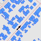
 \begin{overpic}[width=193.77362pt]{figures/qualitative_camera-ready_supp/kitti_2011_09_29_2011_09_29_drive_0071_sync_image_02_data_0000000724.png_image.jpg}\put(5.0,2.0){\color[rgb]{1,1,1}\definecolor[named]{pgfstrokecolor}{rgb}{1,1,1}\pgfsys@color@gray@stroke{1}\pgfsys@color@gray@fill{1}\scriptsize$\Delta\bm{\mathrm{\xi}}{=}2.1\text{m}/0.8\degree\quad{\Delta\text{lateral}}{=}0.3\text{m}\quad{\Delta\text{long.}}{=}2.1\text{m}$}
\end{overpic}
 \begin{overpic}[width=193.77362pt]{figures/qualitative_camera-ready_supp/kitti_2011_10_03_2011_10_03_drive_0027_sync_image_02_data_0000000523.png_image.jpg}\put(5.0,2.0){\color[rgb]{1,1,1}\definecolor[named]{pgfstrokecolor}{rgb}{1,1,1}\pgfsys@color@gray@stroke{1}\pgfsys@color@gray@fill{1}\scriptsize$\Delta\bm{\mathrm{\xi}}{=}0.5\text{m}/1.9\degree\quad{\Delta\text{lateral}}{=}0.3\text{m}\quad{\Delta\text{long.}}{=}0.4\text{m}$}
\end{overpic}
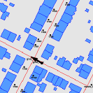
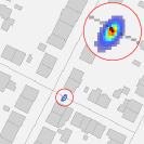
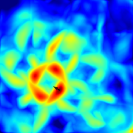

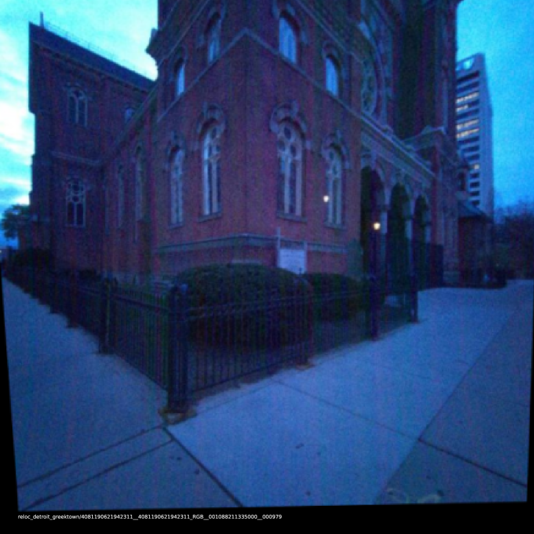
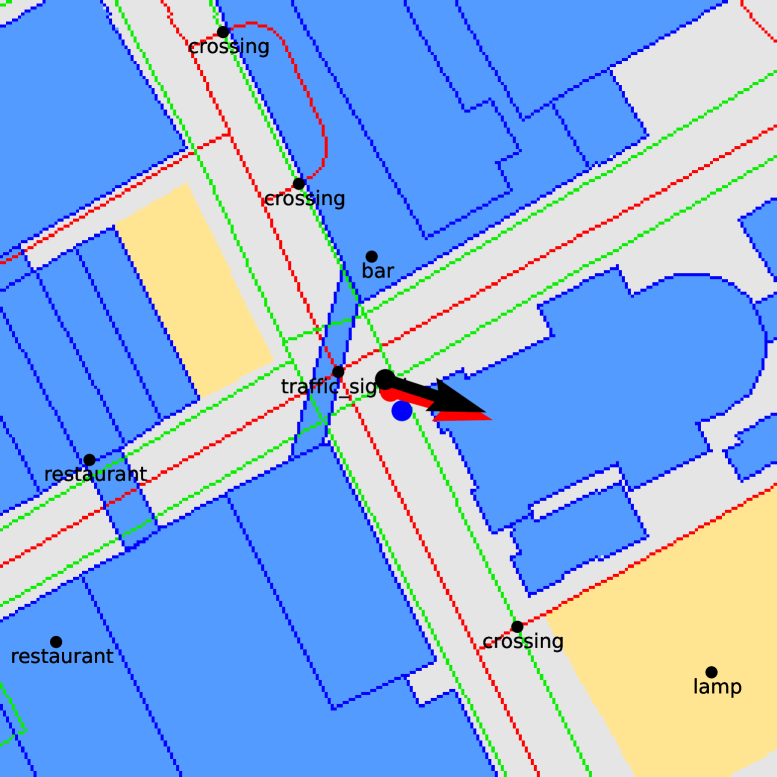
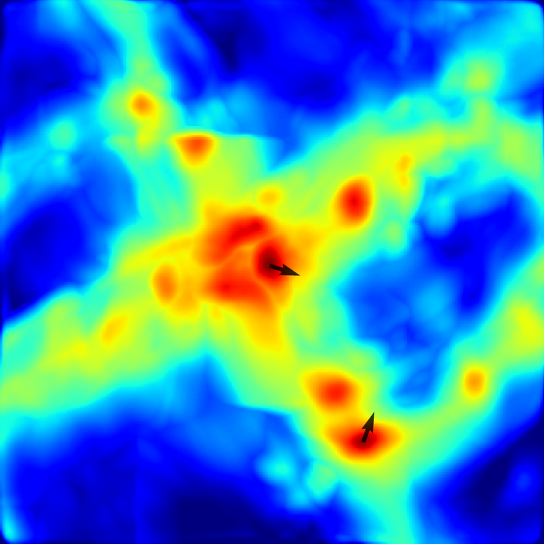
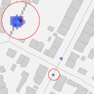
Map legend: building area and outline, road, footway, cycleway, grass, park, playground, parking, fence
 ) along with the ground truth pose (red arrow).
For Aria data, we also show the noisy GPS measurement as a blue dot .
gravity-aligned image
input map
likelihood
log-likelihood
neural map
Hand-held (MGL)
width 1pt
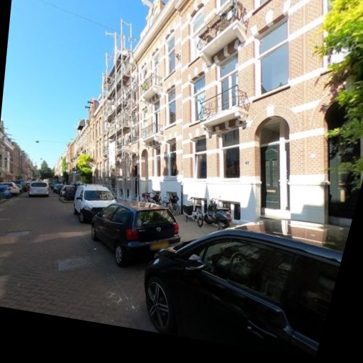
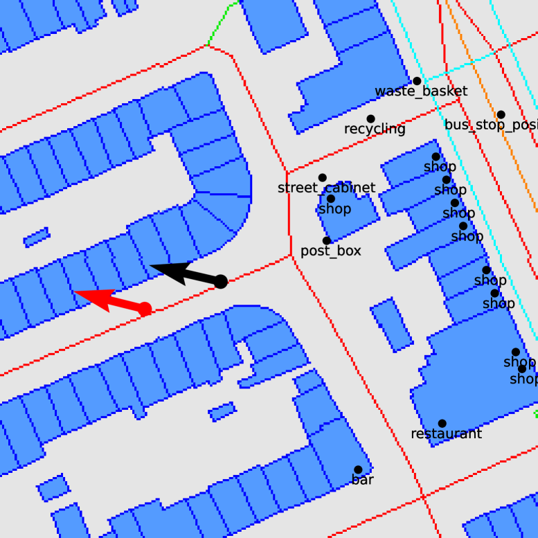 \begin{overpic}[width=405.43362pt]{figures/qualitative_camera-ready_supp_failures/amsterdam_FvjZfvk3z6A0pptMQoNnXl_front_likelihood.pdf}
\put(5.0,5.0){\color[rgb]{0,0,0}\definecolor[named]{pgfstrokecolor}{rgb}{0,0,0}\pgfsys@color@gray@stroke{0}\pgfsys@color@gray@fill{0}\scriptsize$\Delta\bm{\mathrm{\xi}}{=}19.2\text{m}/1.0\degree$}
\end{overpic}
 \begin{overpic}[width=405.43362pt]{figures/qualitative_camera-ready_supp_failures/helsinki_Z4urNDUJ9lc6zCqoswEp8R_right_likelihood.pdf}\put(5.0,5.0){\color[rgb]{0,0,0}\definecolor[named]{pgfstrokecolor}{rgb}{0,0,0}\pgfsys@color@gray@stroke{0}\pgfsys@color@gray@fill{0}\scriptsize$\Delta\bm{\mathrm{\xi}}{=}7.3\text{m}/1.1\degree$}
\end{overpic}
Head-mounted (Aria)
width 1pt

 \begin{overpic}[width=405.43362pt]{figures/qualitative_camera-ready_supp_failures/reloc_detroit_gcp_4185600148151423__4185600148151423_RGB__000629731977000__000571_likelihood.pdf}\put(5.0,5.0){\color[rgb]{0,0,0}\definecolor[named]{pgfstrokecolor}{rgb}{0,0,0}\pgfsys@color@gray@stroke{0}\pgfsys@color@gray@fill{0}\scriptsize$\Delta\bm{\mathrm{\xi}}{=}18.8\text{m}/177.1\degree$}
\put(5.0,15.0){\color[rgb]{0,0,0}\definecolor[named]{pgfstrokecolor}{rgb}{0,0,0}\pgfsys@color@gray@stroke{0}\pgfsys@color@gray@fill{0}\scriptsize$\Delta\text{GPS}{=}18.7\text{m}$}
\end{overpic}


 \begin{overpic}[width=405.43362pt]{figures/qualitative_camera-ready_supp_failures/reloc_seattle_downtown_362038735116186__362038735116186_RGB__000106020981000__000007_likelihood.pdf}\put(5.0,5.0){\color[rgb]{0,0,0}\definecolor[named]{pgfstrokecolor}{rgb}{0,0,0}\pgfsys@color@gray@stroke{0}\pgfsys@color@gray@fill{0}\scriptsize$\Delta\bm{\mathrm{\xi}}{=}33.3\text{m}/4.3\degree$}
\put(5.0,15.0){\color[rgb]{0,0,0}\definecolor[named]{pgfstrokecolor}{rgb}{0,0,0}\pgfsys@color@gray@stroke{0}\pgfsys@color@gray@fill{0}\scriptsize$\Delta\text{GPS}{=}18.2\text{m}$}
\end{overpic}

Car-mounted (KITTI)
width 1pt
\begin{overpic}[width=193.77362pt]{figures/qualitative_camera-ready_supp_failures/kitti_2011_09_26_2011_09_26_drive_0101_sync_image_02_data_0000000532.png_image.jpg}\put(5.0,2.0){\color[rgb]{1,1,1}\definecolor[named]{pgfstrokecolor}{rgb}{1,1,1}\pgfsys@color@gray@stroke{1}\pgfsys@color@gray@fill{1}\scriptsize$\Delta\bm{\mathrm{\xi}}{=}55.2\text{m}/127.6\degree\quad{\Delta\text{lateral}}{=}53.8\text{m}\quad{\Delta\text{long.}}{=}12.5\text{m}$}
\end{overpic}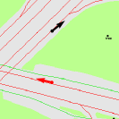
 \begin{overpic}[width=193.77362pt]{figures/qualitative_camera-ready_supp_failures/kitti_2011_09_30_2011_09_30_drive_0020_sync_image_02_data_0000000126.png_image.jpg}\put(5.0,2.0){\color[rgb]{1,1,1}\definecolor[named]{pgfstrokecolor}{rgb}{1,1,1}\pgfsys@color@gray@stroke{1}\pgfsys@color@gray@fill{1}\scriptsize$\Delta\bm{\mathrm{\xi}}{=}14.9\text{m}/0.5\degree\quad{\Delta\text{lateral}}{=}0.6\text{m}\quad{\Delta\text{long.}}{=}14.8\text{m}$}
\end{overpic}
 \begin{overpic}[width=193.77362pt]{figures/qualitative_camera-ready_supp_failures/kitti_2011_10_03_2011_10_03_drive_0027_sync_image_02_data_0000000087.png_image.jpg}\put(5.0,2.0){\color[rgb]{1,1,1}\definecolor[named]{pgfstrokecolor}{rgb}{1,1,1}\pgfsys@color@gray@stroke{1}\pgfsys@color@gray@fill{1}\scriptsize$\Delta\bm{\mathrm{\xi}}{=}24.0\text{m}/176.6\degree\quad{\Delta\text{lateral}}{=}0.5\text{m}\quad{\Delta\text{long.}}{=}24.0\text{m}$}
\end{overpic}
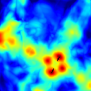

Map legend: building area and outline, road, footway, cycleway, grass, park, playground, parking, fence
Acknowledgments: Thanks to Yann Noutary, Manuel López Antequera, Aleksander Colovic, and Arno Knapitsch for assisting with using OpenSfM and Mapillary data. Thanks to Silvan Weder, Songyou Peng, and the anonymous reviewers for their thoughtful comments.
Appendix
Appendix A Additional results
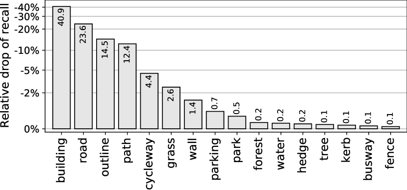
Which map elements are most important? We study in Fig. 10 the impact of each type of map element on the final accuracy by dropping them from the input map. The classes with the largest impact are buildings and road, which are also the most common in areas covered by the training data.
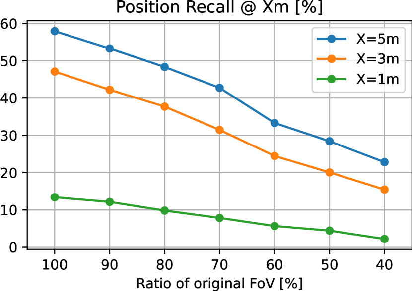
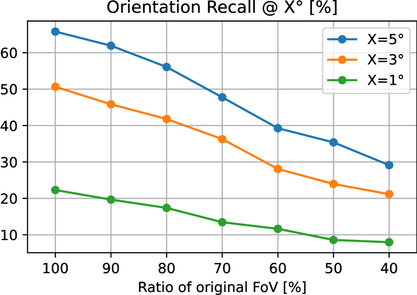
Impact of the field-of-view: We study the impact of the FoV on the accuracy by cropping the images in the horizontal direction to varying degrees. Figure 11 shows the results on the MGL validation set. Reducing the FoV decreases the accuracy proportionally – a 50% smaller FoV results in half of the original accuracy.
Appendix B Data processing and distribution
B.1 OpenStreetMap
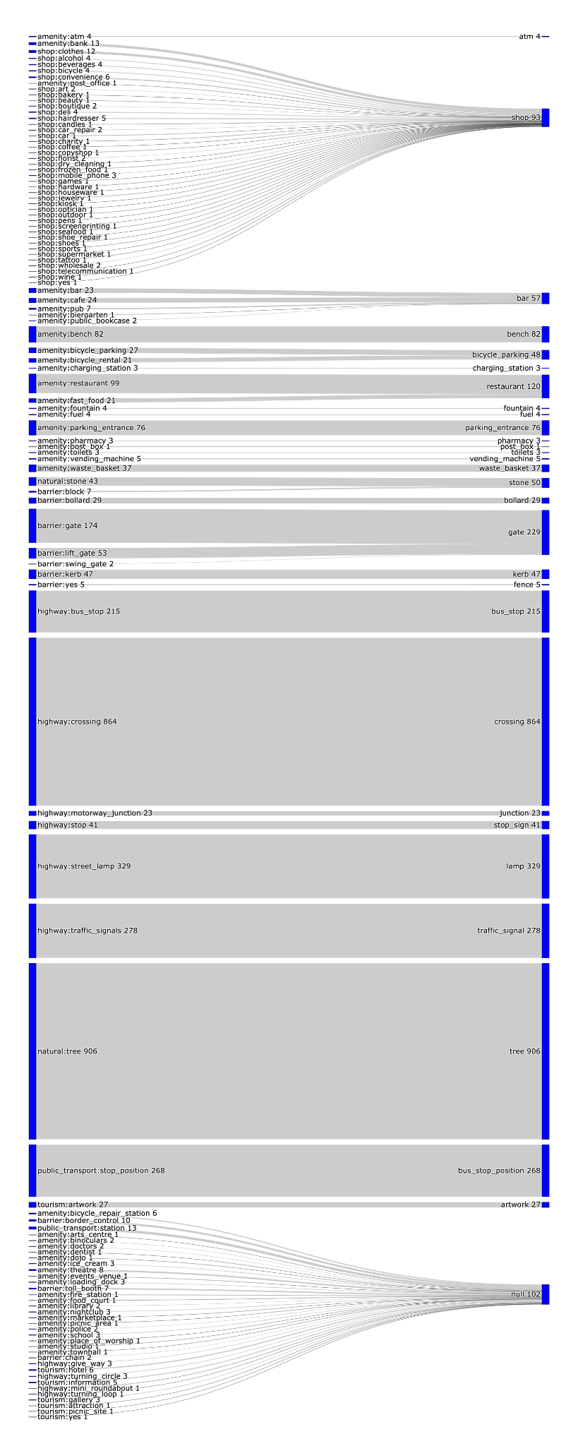
Map classes: OpenStreetMap [46] exposes for each element a set of tags with standardized categories and labels according to a very rich hierarchy. We group elements into a smaller set of classes that we list in Tab. 5, resulting in 7 types of areas, 10 types of lines, and 33 types of points (nodes). Figure 14 shows the distribution of such elements for a small area. Figure 15 shows how some OSM tags are mapped to some semantic classes.
Coordinate system: The coordinates of the map elements are given in WGS84 coordinates (longitude and latitude). We convert them to a local scaled Mercator datum centered at the median camera pose of each area. This yields topocentric coordinates that are aligned with the East and North axes.
B.2 Mapillary Geo-Localization dataset
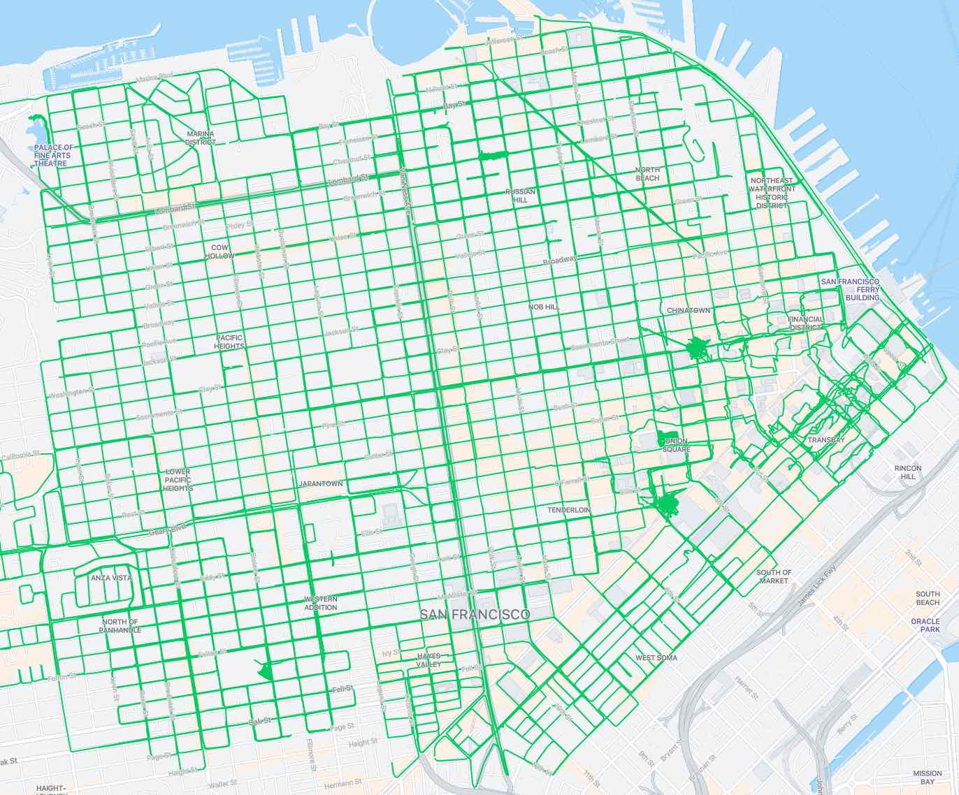
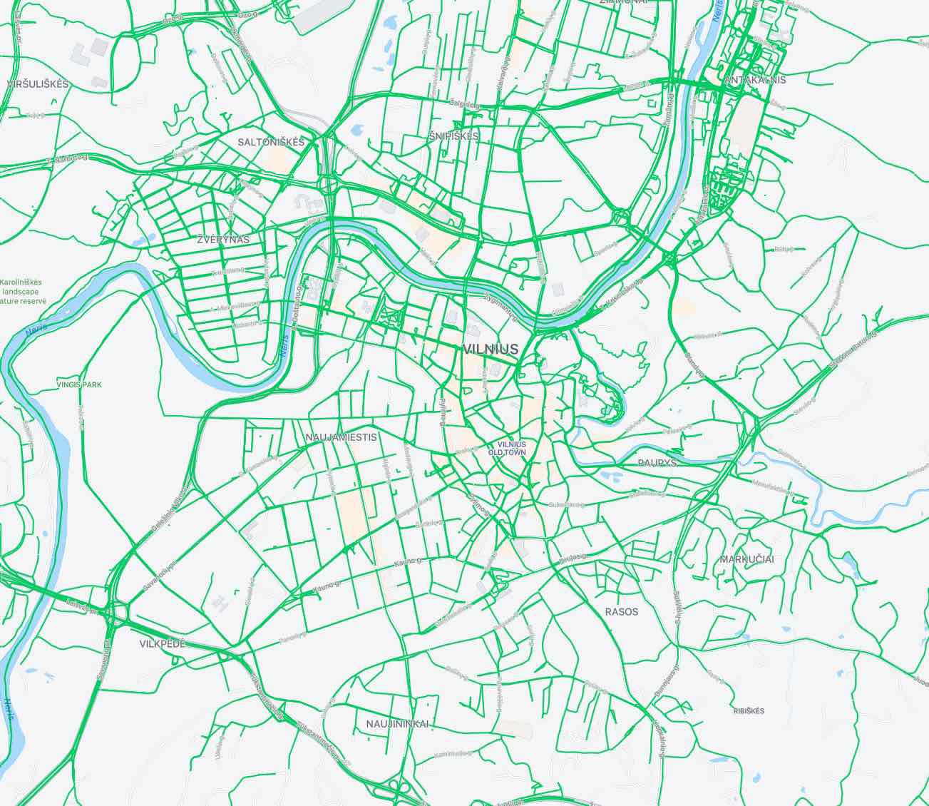
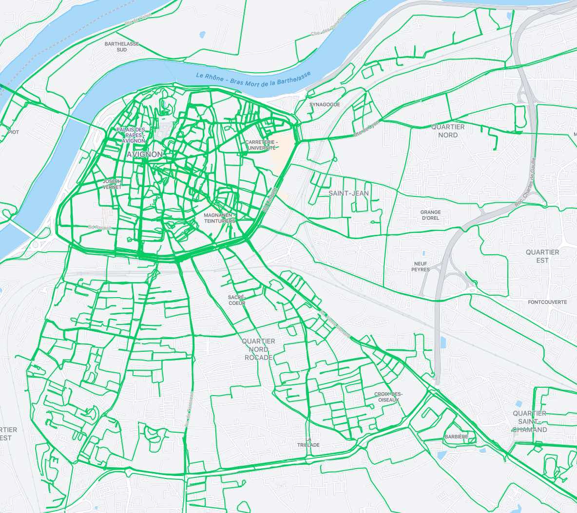
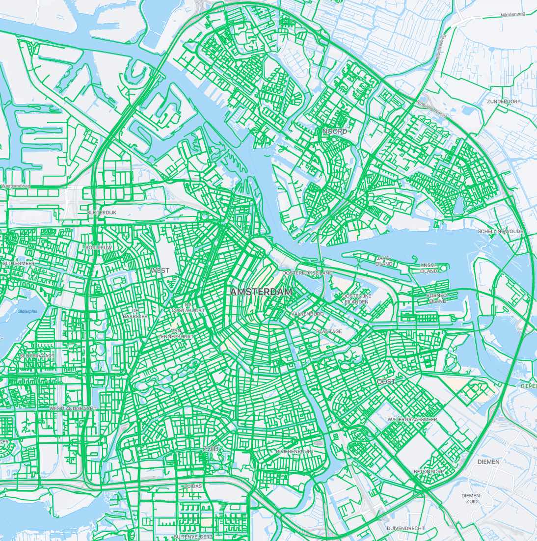
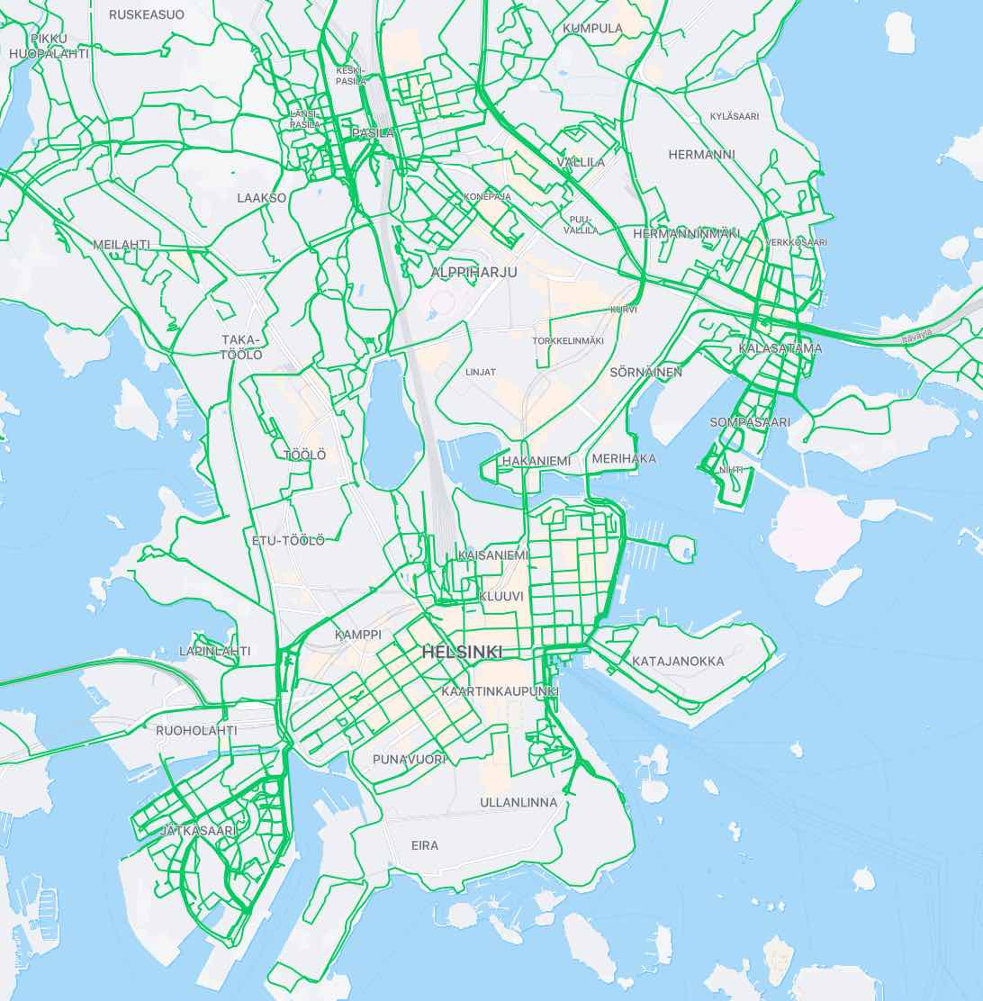
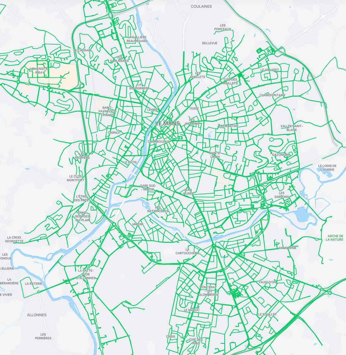
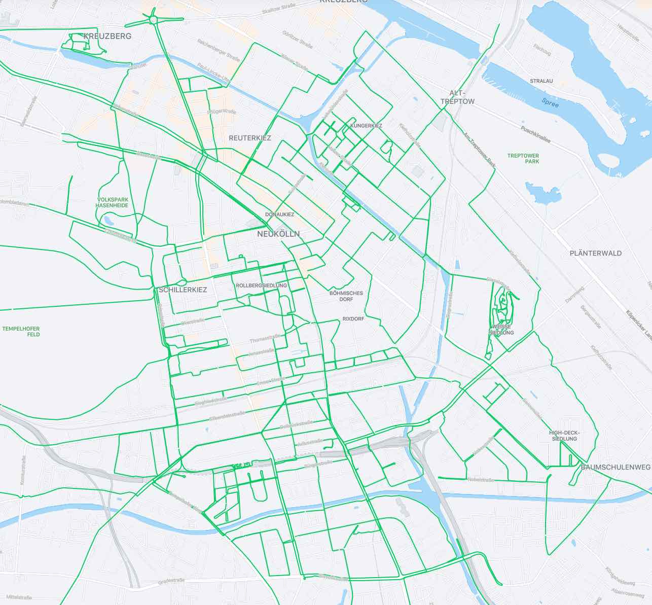
Curation process: We browsed the Mapillary platform and looked for sequences that were sufficiently recent and with the most accurate ground truth poses. We selected sequences recorded after 2017 and with cameras known for resulting in good reconstructions. These include the Xiaomi Yi Action 2K (fisheye) or GoPro Max, MADV QJXJ01FJ, or LG-R105 (spherical) cameras. We selected 12 cities, listed in Tab. 6, that have a high density of such sequences. Figure 13 shows maps overlayed with the selected sequences. Images of each location were split into disjoint training and validation sets, resulting in 826k training and 2k validation views.
Preprocessing: We discard sequences with poor reconstruction statistics or high overlap with OSM building footprints. We subsample the sequences such that frames are spaced by at least 4 meters. We undistorted fisheye images into pinhole cameras. We resampled each 360 panorama into 4 90°-FOV perspective views at equally-distributed yaw angles with a random offset constant per sequence. We query OSM data for each city and create tiles of our raster representation at a resolution .
| type | classes |
| areas | parking spot/lot, building, grass, playground, park, forest, water |
| lines | road, cycleway, pathway, busway, fence, wall, hedge, kerb, building outline, tree row |
| nodes | parking entrance, street lamp, junction, traffic signal, stop sign, give way sign, bus stop, stop area, crossing, gate, bollard, gas station, bicycle parking, charging station, shop, restaurant, bar, vending machine, pharmacy, tree, stone, ATM, toilets, water fountain, bench, waste basket, post box, artwork, recycling station, clock, fire hydrant, pole, street cabinet |
| Country | City | # sequences | # images |
| USA | San Francisco | 1013 | 207.6k |
| Netherlands | Amsterdam | 57 | 72.9k |
| Germany | Berlin | 59 | 54.6k |
| Lithuania | Vilnius | 381 | 111.5k |
| Finland | Helsinki | 91 | 55.4k |
| Italy | Milan | 156 | 46.2k |
| France | Paris | 136 | 68.4k |
| Montrouge | 159 | 33.3k | |
| Le Mans | 111 | 27.4k | |
| Nantes | 171 | 62.5k | |
| Avignon | 160 | 75.2k | |
| Toulouse | 86 | 39.6k |
B.3 Aria datasets
Recording: We recorded data with Aria devices [1] at 3 locations in Seattle (Downtown, Pike Place Market, Westlake) and at 2 locations in Detroit (Greektown, Grand Circus Park). In each location, we recorded 3 to 5 sequences following the same trajectories, for a duration of 5 to 25 minutes varying by location. Each device is equipped with a consumer-grade GPS sensor, IMUs, grayscale SLAM cameras, and a front-facing RGB camera, which we undistort to a pinhole model.
Evaluation: We associate GPS signals captured at 1Hz with undistorted RGB images keyframed at 3 meters. This resulted in 2153 frames for Seattle and 2725 frames for Detroit. For each evaluation example, the map tile is centered around the noisy GPS measurement. Because of large differences in GPS accuracy due to urban canyons, we constrain the predictions within of the measurement for Seattle and for Detroit.
Comparison to feature matching: Algorithms based on 3D SfM maps require mapping images, whose quality and density have a large impact on the localization accuracy. Differently, OrienterNet can localize in areas not covered by such images as long as OSM data is available. This makes any fair comparison difficult.
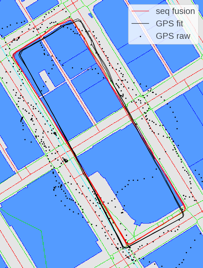
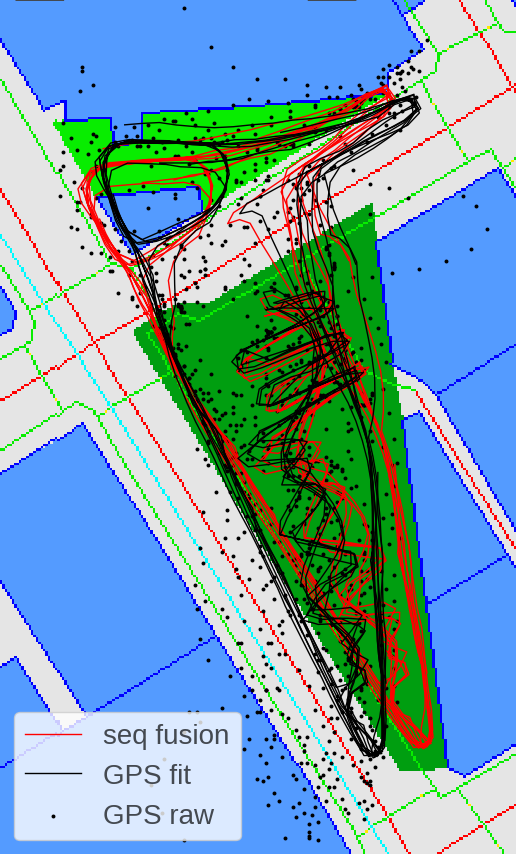
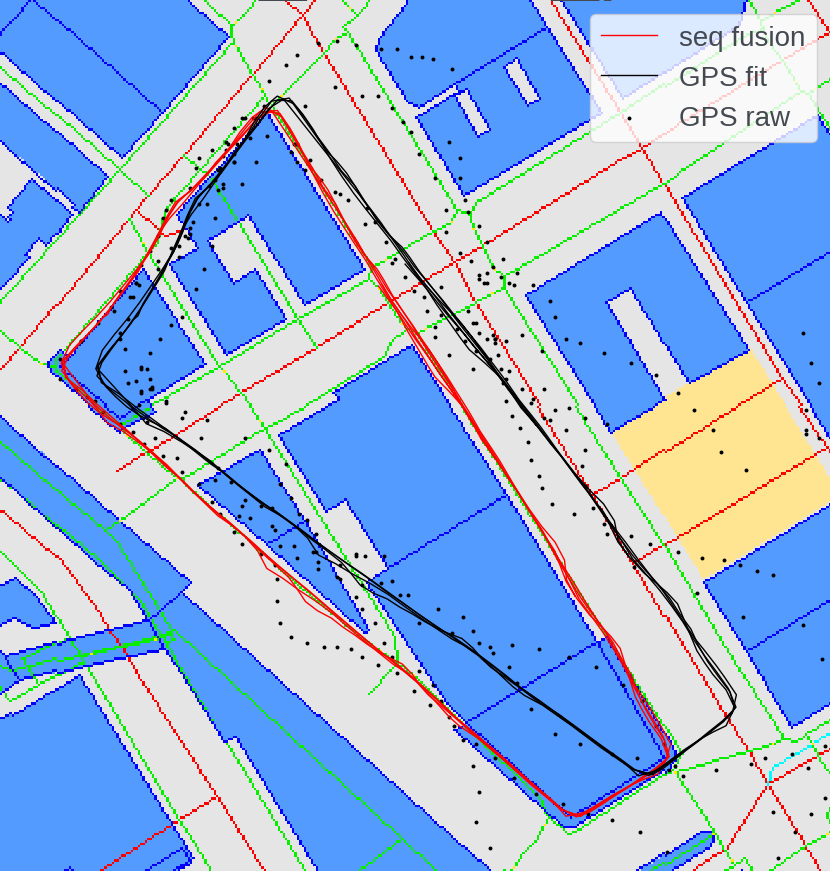
Geo-alignment: Evaluating the localization within world-aligned maps requires the geo-alignement between each device pose and the global reference frame. We first co-register all trajectories of each location by minimizing visual-inertial SLAM constraints, which yields consistent poses in a local reference frame that is gravity-aligned and at metric scale. We then find the global 3-DoF rigid transformation by fusing all GPS signals with the predictions of OrienterNet for each image. To do, we perform iterative truncated least-squares, annealing the outlier threshold from 5m to 1m.
We show visualizations of this alignment in Fig. 12. While GPS signals are too noisy to reliably fit a transformation, OrienterNet provides complementary and accurate local constraints. We visually check that the final alignment error is lower than 1m, which is sufficient for our evaluation.
Downtown
Westlake
Pike Central Market
Appendix C Implementation details
Orienter-Net: To save GPU memory, we use only rotation bins at training time but increase it to at test time. BEV and map features have channels. To avoid overfitting, we found it critical to use replicate padding in the map-CNN and to apply data augmentation to the raster map by randomly flipping and rotating it. We also use replicate padding in the BEV-to-map matching operation to avoid biasing the predictions near the map boundaries. The scale boundaries and are set to and , respectively. For the median focal length of the MGL training set, this corresponds to a depth interval of .
Training images are resized to pixels. When evaluating on KITTI and Aria data, images are resized such that their focal length is . We train with a batch size of 9 over 3 V100 GPUs with 16GB VRAM each. We select the best model checkpoint with early stopping based on the validation loss.
Retrieval baseline: The work of Samano et al. [56] infers a global descriptor for each map patch. This is inefficient when considering densely sampled areas. We can equivalently predict a dense feature map in one CNN forward pass, which is similar to the recent work of Xia et al. [77] for satellite imagery. We then correlate the global image descriptor with to obtain the pixelwise log-score . To predict a rotation, computes 4 feature maps for the 4 N-S-E-W directions, from which we can linearly interpolate map features for any number of rotation bins This yields a 3D pose volume as for OrienterNet. We found this approach much more efficient than re-computing map features for different map orientations.
Refinement baseline: We follow the official implementation of Shi et al. [62] with multi-level optimization at each iteration and warm restart. We supervise the longitudinal, lateral, and angular offsets with an L2 loss at each iteration and scale. The map data and branch are identical to OrienterNet.
San Francisco
Vilnius
Avignon
Amsterdam
Helsinki
Le Mans
Berlin
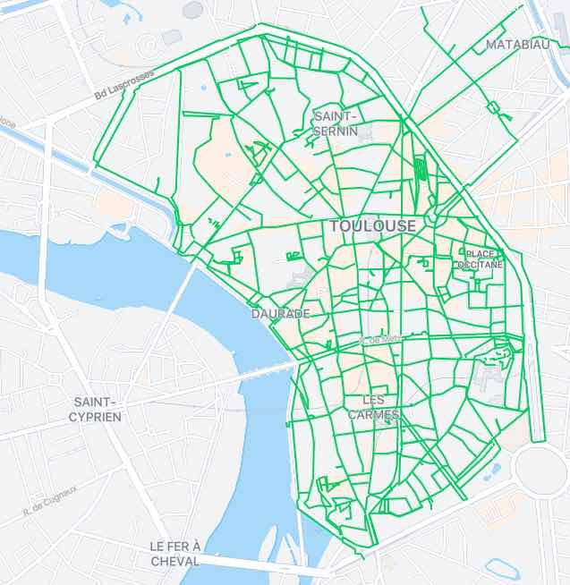
Toulouse
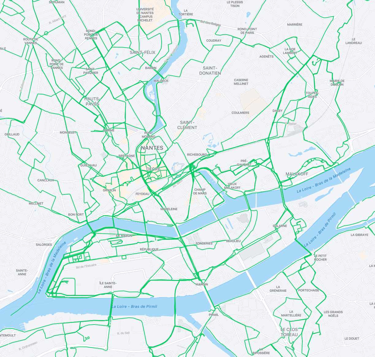
Nantes
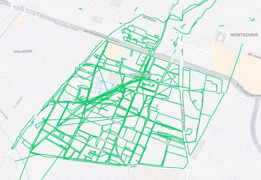
Montrouge
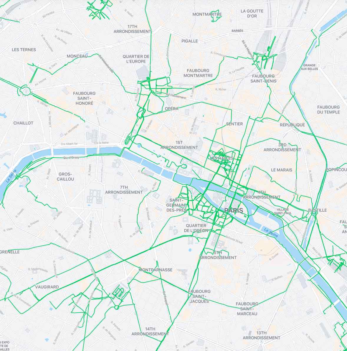
Paris
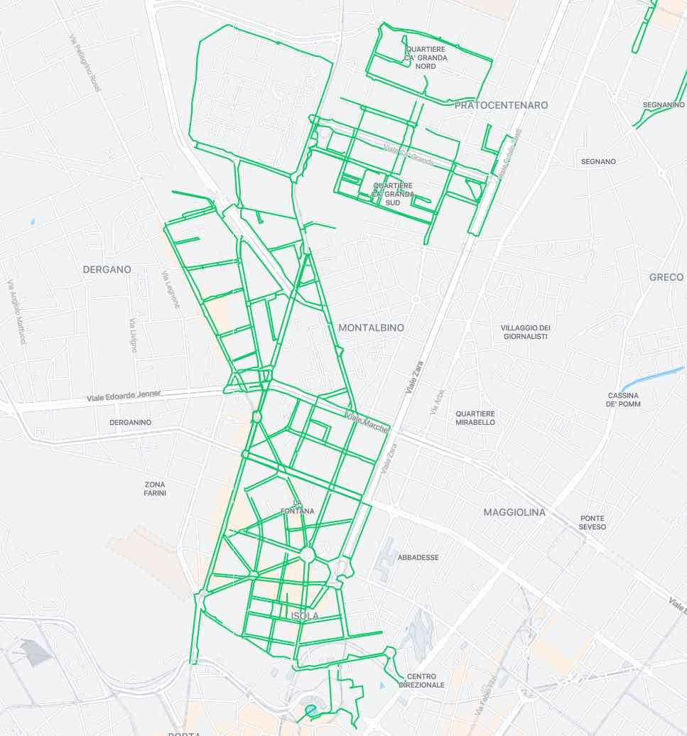
Milan


References
- [1] Project Aria. https://about.facebook.com/realitylabs/projectaria/, 2022.
- [2] Sameer Agarwal, Yasutaka Furukawa, Noah Snavely, Ian Simon, Brian Curless, Steven M Seitz, and Richard Szeliski. Building Rome in a day. Communications of the ACM, 54(10):105–112, 2011.
- [3] Manuel López Antequera, Pau Gargallo, Markus Hofinger, Samuel Rota Bulò, Yubin Kuang, and Peter Kontschieder. Mapillary planet-scale depth dataset. In ECCV, 2020.
- [4] Relja Arandjelovic, Petr Gronat, Akihiko Torii, Tomas Pajdla, and Josef Sivic. NetVLAD: CNN architecture for weakly supervised place recognition. In CVPR, 2016.
- [5] Anil Armagan, Martin Hirzer, Peter M Roth, and Vincent Lepetit. Accurate camera registration in urban environments using high-level feature matching. In BMVC, 2017.
- [6] Anil Armagan, Martin Hirzer, Peter M Roth, and Vincent Lepetit. Learning to align semantic segmentation and 2.5D maps for geolocalization. In CVPR, 2017.
- [7] Dan Barnes, Rob Weston, and Ingmar Posner. Masking by moving: Learning distraction-free radar odometry from pose information. In CoRL, 2020.
- [8] Ioan Andrei Barsan, Shenlong Wang, Andrei Pokrovsky, and Raquel Urtasun. Learning to localize using a lidar intensity map. In CoRL, 2018.
- [9] Herbert Bay, Tinne Tuytelaars, and Luc Van Gool. SURF: Speeded up robust features. In ECCV, 2006.
- [10] Martin Bujnak, Zuzana Kukelova, and Tomas Pajdla. A general solution to the p4p problem for camera with unknown focal length. In CVPR, 2008.
- [11] Wolfram Burgard, Dieter Fox, Daniel Hennig, and Timo Schmidt. Estimating the absolute position of a mobile robot using position probability grids. In AAAI, 1996.
- [12] Federico Camposeco, Andrea Cohen, Marc Pollefeys, and Torsten Sattler. Hybrid scene compression for visual localization. In CVPR, June 2019.
- [13] Song Cao and Noah Snavely. Minimal scene descriptions from structure from motion models. In CVPR, 2014.
- [14] Francesco Castaldo, Amir Zamir, Roland Angst, Francesco Palmieri, and Silvio Savarese. Semantic cross-view matching. In ICCV Workshop on Vision from Satellite to Street, 2015.
- [15] Tat-Jen Cham, Arridhana Ciptadi, Wei-Chian Tan, Minh-Tri Pham, and Liang-Tien Chia. Estimating camera pose from a single urban ground-view omnidirectional image and a 2D building outline map. In CVPR, 2010.
- [16] Hang Chu, Andrew Gallagher, and Tsuhan Chen. GPS refinement and camera orientation estimation from a single image and a 2D map. In CVPR Workshops, 2014.
- [17] Philip David and Sean Ho. Orientation descriptors for localization in urban environments. In IROS, 2011.
- [18] Daniel DeTone, Tomasz Malisiewicz, and Andrew Rabinovich. SuperPoint: Self-supervised interest point detection and description. In CVPR Workshop on Deep Learning for Visual SLAM, 2018.
- [19] Mihai Dusmanu, Ignacio Rocco, Tomas Pajdla, Marc Pollefeys, Josef Sivic, Akihiko Torii, and Torsten Sattler. D2-Net: A trainable CNN for joint detection and description of local features. In CVPR, 2019.
- [20] Mihai Dusmanu, Johannes L. Schönberger, Sudipta N. Sinha, and Marc Pollefeys. Privacy-Preserving Image Features via Adversarial Affine Subspace Embeddings. In CVPR, 2021.
- [21] Georgios Floros, Benito van der Zander, and Bastian Leibe. OpenStreetSLAM: Global vehicle localization using OpenStreetMaps. In ICRA, 2013.
- [22] Jan-Michael Frahm, Pierre Fite-Georgel, David Gallup, Tim Johnson, Rahul Raguram, Changchang Wu, Yi-Hung Jen, Enrique Dunn, Brian Clipp, Svetlana Lazebnik, et al. Building Rome on a cloudless day. In ECCV, 2010.
- [23] Dorian Galvez-López and Juan D. Tardos. Bags of binary words for fast place recognition in image sequences. IEEE Transactions on Robotics, 28(5):1188–1197, 2012.
- [24] Andreas Geiger, Philip Lenz, Christoph Stiller, and Raquel Urtasun. Vision meets robotics: The KITTI dataset. The International Journal of Robotics Research, 32(11):1231–1237, 2013.
- [25] Chengcheng Guo, Minjie Lin, Heyang Guo, Pengpeng Liang, and Erkang Cheng. Coarse-to-fine semantic localization with HD map for autonomous driving in structural scenes. In IROS, 2021.
- [26] R.M. Haralick, C.-N. Lee, K. Ottenberg, and M. Nölle. Review and analysis of solutions of the three point perspective pose estimation problem. IJCV, 13(3):331–356, 1994.
- [27] Ziyang Hong, Yvan Petillot, David Lane, Yishu Miao, and Sen Wang. TextPlace: Visual place recognition and topological localization through reading scene texts. In ICCV, 2019.
- [28] Henry Howard-Jenkins, Jose-Raul Ruiz-Sarmiento, and Victor Adrian Prisacariu. Lalaloc: Latent layout localisation in dynamic, unvisited environments. In CVPR, 2021.
- [29] Lukas Hoyer, Dengxin Dai, Yuhua Chen, Adrian Koring, Suman Saha, and Luc Van Gool. Three ways to improve semantic segmentation with self-supervised depth estimation. In CVPR, 2021.
- [30] Sixing Hu, Mengdan Feng, Rang M. H. Nguyen, and Gim Hee Lee. CVM-Net: Cross-view matching network for image-based ground-to-aerial geo-localization. In CVPR, 2018.
- [31] Arnold Irschara, Christopher Zach, Jan-Michael Frahm, and Horst Bischof. From structure-from-motion point clouds to fast location recognition. In CVPR, 2009.
- [32] Hervé Jégou, Matthijs Douze, Cordelia Schmid, and Patrick Pérez. Aggregating local descriptors into a compact image representation. In CVPR, 2010.
- [33] L Kneip, D Scaramuzza, and R Siegwart. A Novel Parametrization of the Perspective-Three-Point Problem for a Direct Computation of Absolute Camera Position and Orientation. In CVPR, 2011.
- [34] Dong Lao, Alex Wong, and Stefano Soatto. Does monocular depth estimation provide better pre-training than classification for semantic segmentation? arXiv:2203.13987, 2022.
- [35] Viktor Larsson, Marc Pollefeys, and Magnus Oskarsson. Orthographic-perspective epipolar geometry. In ICCV, 2021.
- [36] Philipp Lindenberger, Paul-Edouard Sarlin, Viktor Larsson, and Marc Pollefeys. Pixel-Perfect Structure-from-Motion with Featuremetric Refinement. In ICCV, 2021.
- [37] Amy K Lobben. Navigational map reading: Predicting performance and identifying relative influence of map-related abilities. Annals of the association of American geographers, 97(1):64–85, 2007.
- [38] David G Lowe. Distinctive image features from scale-invariant keypoints. IJCV, 60(2):91–110, 2004.
- [39] Simon Lynen, Bernhard Zeisl, Dror Aiger, Michael Bosse, Joel Hesch, Marc Pollefeys, Roland Siegwart, and Torsten Sattler. Large-scale, real-time visual-inertial localization revisited. IJRR, 39(9):1061–1084, 2020.
- [40] Wei-Chiu Ma, Ignacio Tartavull, Ioan Andrei Bârsan, Shenlong Wang, Min Bai, Gellert Mattyus, Namdar Homayounfar, Shrinidhi Kowshika Lakshmikanth, Andrei Pokrovsky, and Raquel Urtasun. Exploiting sparse semantic HD maps for self-driving vehicle localization. In IROS, 2019.
- [41] Wei-Chiu Ma, Shenlong Wang, Marcus A. Brubaker, Sanja Fidler, and Raquel Urtasun. Find your way by observing the sun and other semantic cues. In ICRA, 2017.
- [42] Zhixiang Min, Naji Khosravan, Zachary Bessinger, Manjunath Narayana, Sing Bing Kang, Enrique Dunn, and Ivaylo Boyadzhiev. Laser: Latent space rendering for 2d visual localization. In CVPR, 2022.
- [43] Pierre Moulon, Pascal Monasse, Romuald Perrot, and Renaud Marlet. OpenMVG: Open multiple view geometry. In International Workshop on Reproducible Research in Pattern Recognition, pages 60–74. Springer, 2016.
- [44] Tony Ng, Hyo Jin Kim, Vincent T. Lee, Daniel DeTone, Tsun-Yi Yang, Tianwei Shen, Eddy Ilg, Vassileios Balntas, Krystian Mikolajczyk, and Chris Sweeney. NinjaDesc: Content-concealing visual descriptors via adversarial learning. In CVPR, 2022.
- [45] J. O’Keefe and L. Nadel. The hippocampus as a cognitive map. Clarendon Press, 1978.
- [46] OpenStreetMap contributors. Planet dump retrieved from https://planet.osm.org . https://www.openstreetmap.org, 2017.
- [47] Pilailuck Panphattarasap and Andrew Calway. Automated map reading: image based localisation in 2-D maps using binary semantic descriptors. In IROS, 2018.
- [48] Jan-Hendrik Pauls, Kürsat Petek, Fabian Poggenhans, and Christoph Stiller. Monocular localization in HD maps by combining semantic segmentation and distance transform. In IROS, 2020.
- [49] Jonah Philion and Sanja Fidler. Lift, splat, shoot: Encoding images from arbitrary camera rigs by implicitly unprojecting to 3d. In ECCV, 2020.
- [50] Francesco Pittaluga, Sanjeev J Koppal, Sing Bing Kang, and Sudipta N Sinha. Revealing scenes by inverting structure from motion reconstructions. In CVPR, 2019.
- [51] Jerome Revaud, Philippe Weinzaepfel, César De Souza, Noe Pion, Gabriela Csurka, Yohann Cabon, and Martin Humenberger. R2D2: Repeatable and reliable detector and descriptor. In NeurIPS, 2019.
- [52] Thomas Roddick and Roberto Cipolla. Predicting semantic map representations from images using pyramid occupancy networks. In CVPR, 2020.
- [53] Ethan Rublee, Vincent Rabaud, Kurt Konolige, and Gary R Bradski. ORB: An efficient alternative to SIFT or SURF. In ICCV, 2011.
- [54] Philipp Ruchti, Bastian Steder, Michael Ruhnke, and Wolfram Burgard. Localization on OpenStreetMap data using a 3d laser scanner. In ICRA, 2015.
- [55] Avishkar Saha, Oscar Mendez, Chris Russell, and Richard Bowden. Translating images into maps. In ICRA, 2022.
- [56] Noe Samano, Mengjie Zhou, and Andrew Calway. You are here: Geolocation by embedding maps and images. In ECCV, 2020.
- [57] Paul-Edouard Sarlin, Cesar Cadena, Roland Siegwart, and Marcin Dymczyk. From coarse to fine: Robust hierarchical localization at large scale. In CVPR, 2019.
- [58] Paul-Edouard Sarlin, Daniel DeTone, Tomasz Malisiewicz, and Andrew Rabinovich. SuperGlue: Learning feature matching with graph neural networks. In CVPR, 2020.
- [59] Paul-Edouard Sarlin, Ajaykumar Unagar, Måns Larsson, Hugo Germain, Carl Toft, Viktor Larsson, Marc Pollefeys, Vincent Lepetit, Lars Hammarstrand, Fredrik Kahl, and Torsten Sattler. Back to the Feature: Learning robust camera localization from pixels to pose. In CVPR, 2021.
- [60] Torsten Sattler, Bastian Leibe, and Leif Kobbelt. Improving image-based localization by active correspondence search. In ECCV, 2012.
- [61] Johannes Lutz Schönberger and Jan-Michael Frahm. Structure-from-motion revisited. In CVPR, 2016.
- [62] Yujiao Shi and Hongdong Li. Beyond cross-view image retrieval: Highly accurate vehicle localization using satellite image. In CVPR, 2022.
- [63] Yujiao Shi, Liu Liu, Xin Yu, and Hongdong Li. Spatial-aware feature aggregation for image based cross-view geo-localization. In NeurIPS, 2019.
- [64] Yujiao Shi, Xin Yu, Dylan Campbell, and Hongdong Li. Where am I looking at? joint location and orientation estimation by cross-view matching. In CVPR, 2020.
- [65] Yujiao Shi, Xin Yu, Liu Liu, Tong Zhang, and Hongdong Li. Optimal feature transport for cross-view image geo-localization. In AAAI, 2020.
- [66] Reid G. Simmons and Sven Koenig. Probabilistic robot navigation in partially observable environments. In IJCAI, 1995.
- [67] Noah Snavely, Steven M Seitz, and Richard Szeliski. Photo Tourism: exploring photo collections in 3D. In SIGGRAPH, 2006.
- [68] Pablo Speciale, Johannes L. Schönberger, Sing Bing Kang, Sudipta N. Sinha, and Marc Pollefeys. Privacy preserving image-based localization. In CVPR, 2019.
- [69] Pablo Speciale, Johannes L. Schönberger, Sudipta N. Sinha, and Marc Pollefeys. Privacy preserving image queries for camera localization. In ICCV, 2019.
- [70] Linus Svärm, Olof Enqvist, Fredrik Kahl, and Magnus Oskarsson. City-scale localization for cameras with known vertical direction. TPAMI, 2017.
- [71] Tim Y. Tang, Daniele De Martini, Shangzhe Wu, and Paul Newman. Self-supervised learning for using overhead imagery as maps in outdoor range sensor localization. IJRR, 40(12-14):1488–1509, 2021.
- [72] Akihiko Torii, Relja Arandjelovic, Josef Sivic, Masatoshi Okutomi, and Tomas Pajdla. 24/7 place recognition by view synthesis. In CVPR, 2015.
- [73] Michał J Tyszkiewicz, Pascal Fua, and Eduard Trulls. DISK: Learning local features with policy gradient. In NeurIPS, 2020.
- [74] Tomas Vojir, Ignas Budvytis, and Roberto Cipolla. Efficient large-scale semantic visual localization in 2D maps. In ACCV, 2020.
- [75] Olga Vysotska and Cyrill Stachniss. Improving SLAM by exploiting building information from publicly available maps and localization priors. PFG–Journal of Photogrammetry, Remote Sensing and Geoinformation Science, 85(1):53–65, 2017.
- [76] Li Weng, Valérie Gouet-Brunet, and Bahman Soheilian. Semantic signatures for large-scale visual localization. Multimedia Tools and Applications, 2021.
- [77] Zimin Xia, Olaf Booij, Marco Manfredi, and Julian FP Kooij. Visual cross-view metric localization with dense uncertainty estimates. In ECCV, 2022.
- [78] Fan Yan, Olga Vysotska, and Cyrill Stachniss. Global localization on OpenStreetMap using 4-bit semantic descriptors. In ECMR, 2019.
- [79] Bernhard Zeisl, Torsten Sattler, and Marc Pollefeys. Camera pose voting for large-scale image-based localization. In ICCV, 2015.
- [80] Mengjie Zhou, Xieyuanli Chen, Noe Samano, Cyrill Stachniss, and Andrew Calway. Efficient localisation using images and OpenStreetMaps. In IROS, 2021.
- [81] Qunjie Zhou, Sergio Agostinho, Aljosa Osep, and Laura Leal-Taixe. Is geometry enough for matching in visual localization? In ECCV, 2022.
- [82] Sijie Zhu, Taojiannan Yang, and Chen Chen. VIGOR: Cross-view image geo-localization beyond one-to-one retrieval. In CVPR, 2021.