Inference of the low-energy constants in delta-full chiral effective field theory including a correlated truncation error

Abstract

We sample the posterior probability distributions of the low-energy constants (LECs) in delta-full chiral effective field theory ($\chi$EFT) up to third order. We use eigenvector continuation for fast and accurate emulation of the likelihood and Hamiltonian Monte Carlo to draw effectively independent samples from the posteriors. Our Bayesian inference is conditioned on the Granada database of neutron-proton ($np$) cross sections and polarizations. We use priors grounded in $\chi$EFT assumptions and a Roy-Steiner analysis of pion-nucleon scattering data. We model correlated EFT truncation errors using a two-feature Gaussian process, and find correlation lengths for $np$ scattering energies and angles in the ranges 40–120 MeV and 25–45 degrees, respectively. These correlations yield a non-diagonal covariance matrix and reduce the number of independent scattering data with a factor of eight and four at the second and third chiral orders, respectively. The relatively small difference between the second and third order predictions in delta-full $\chi$EFT suppresses the marginal variance of the truncation error and the effects of its correlation structure. Our results are particularly important for analyzing the predictive capabilities in ab initio nuclear theory.

I Introduction

A chiral effective field theory ($\chi$EFT) description of the nuclear interaction Weinberg (1990, 1991); Epelbaum et al. (2009); Machleidt and Entem (2011); Hammer et al. (2020) is endowed with a power counting (PC) to organize the order-by-order contributions of the strong-interaction dynamics to nuclear observables. This kind of organization, regardless of the particulars of the adopted PC Yang (2020), is a hallmark of EFT Weinberg (1979) and ab initio Ekström et al. (2023) approaches to nuclear theory since it promises a handle on the theoretical uncertainty coming from truncating the EFT expansion Furnstahl et al. (2015). Accounting for the truncation error is key to mitigate overfitting of the low-energy constants (LECs) as well as assessing the importance of discrepancies. Indeed, the modeling of EFT truncation errors can play a significant role for the robustness of LEC inferences and ensuing nuclear predictions Ekström et al. (2015); Epelbaum et al. (2015); Carlsson et al. (2016); Stroberg et al. (2021); Wesolowski et al. (2021); Jiang et al. (2022a, b). Melendez et al. (2019) have proposed a Bayesian model for the truncation error that accounts for finite correlations across independent variables, e.g., the scattering energy and angle for nucleon-nucleon ($NN$) scattering cross sections and polarizations. To date, LEC inference in $\chi$EFT typically accounts for truncation errors in the limit of zero correlation Melendez et al. (2017); Wesolowski et al. (2016, 2019); Svensson et al. (2022, 2023), and the robustness with respect to the correlation structure is not well known.

In this paper, we quantify a correlated truncation error and analyze its effects on a Bayesian estimation of the LEC posteriors for a $\Delta$-full $\chi$EFT description of the neutron-proton ($np$) interaction up to next-to-next-to-leading order ( NNLO) Krebs et al. (2007); Ekström et al. (2018). This extends our previous work on Bayesian LEC estimation in $\Delta$-less $\chi$EFT where we employed an uncorrelated truncation error Wesolowski et al. (2021); Svensson et al. (2022, 2023). We also use eigenvector continuation (EC) König et al. (2020), i.e., a reduced basis method Melendez et al. (2021), to efficiently and accurately emulate the scattering amplitudes entering the $np$ scattering-data likelihood. Following our previous publications Svensson et al. (2022, 2023), we employ Hamiltonian Monte Carlo (HMC) Duane et al. (1987) to draw effectively independent samples from the LEC posteriors.

The $\Delta(1232)$-resonance plays an important role in nuclear physics since it represents a rather low excitation energy and couples strongly to the pion-nucleon ($\pi N$) system. This was recognized already in early $\chi$EFT descriptions of the $NN$ interaction Ordonez et al. (1994); van Kolck (1994); Ordonez et al. (1996), and several modern $\chi$EFT interactions incorporate the $\Delta$ as well Piarulli et al. (2015, 2016); Logoteta et al. (2016); Jiang et al. (2020). In $\Delta$-full $\chi$EFT  there are four subleading $\pi N$ LECs up to NNLO, usually denoted $c_{1},c_{2},c_{3},c_{4}$. They govern the strength of subleading $2\pi$-exchange diagrams of the $NN$ interaction and the leading three-nucleon ($NNN$) $2\pi$-exchange with an intermediate $\Delta$-excitation, the so-called Fujita-Miyazawa force  Fujita and Miyazawa (1957); Epelbaum et al. (2008). A Roy-Steiner analysis of $\pi N$ scattering amplitudes by Hoferichter et al. (2016) has enabled a determination of the $\pi N$ LECs. Unfortunately, the relatively unknown value of the axial $\pi N\Delta$ coupling $h_{A}$ propagates to approximately five times greater uncertainties for $c_{2},c_{3},c_{4}$ (compared to a determination in $\Delta$-less $\chi$EFT) when matching $\Delta$-full $\chi$EFT to the subthreshold amplitudes in the Roy-Steiner formalism Siemens et al. (2017). A well-founded truncation error would therefore pave the way for learning more about the strength of subleading 2$\pi$-exchange, and leading $NNN$ forces, from $NN$ scattering data.

This paper is organized as follows: In Sec. II we present our statistical model for linking experiment and $\chi$EFT. In Sec. III we discuss our priors and likelihood, and in Sec. IV we introduce the two-feature Gaussian-process model of the correlated EFT truncation error. In Sec. V we discuss the training of EC $np$ scattering emulators. In Sec. VI we present the results from HMC sampling of the LEC posteriors. A summary and an outlook are given in Sec. VII.

II Linking experiment and theory

Following our previous papers Wesolowski et al. (2021); Svensson et al. (2022, 2023), we relate an experimental measurement $y_{\text{exp}}$ of some scattering observable with a theoretical prediction $y_{\text{th}}^{(k)}$, up to chiral order $(k)$, using an additive model to account for the respective uncertainties, $\delta y_{\text{exp}}$ and $\delta y_{\text{th}}^{(k)}$:

$$y_{\text{exp}}(\vec{x})=y_{\text{th}}^{(k)}(\vec{\alpha};\vec{x})+\delta y_{\text{exp}}(\vec{x})+\delta y_{\text{th}}^{(k)}(\vec{x}).$$ (1)

The theory prediction $y_{\text{th}}$ depends deterministically on the vector of LECs $\vec{\alpha}$ and the independent variable $\vec{x}=(T_{\text{lab}},\theta)$, where $T_{\text{lab}}$ denotes the kinetic energy of the incoming nucleon in the laboratory frame and $\theta$ denotes the scattering angle in the center-of-mass frame. For the total scattering cross section we have $\vec{x}=(T_{\text{lab}})$ as this observable is integrated over all $\theta$. We have suppressed the explicit $\vec{\alpha}$-dependence of $\delta y_{\text{th}}^{(k)}$ as we will assume a fixed parameter value in the model of the theory error.

The composition of the LEC vector $\vec{\alpha}$ depends on the chiral order. For the $np$ potentials in this paper, the LEC vector up to each order is given by

$$\vec{\alpha}_{\textnormal{LO}}=\Bigl{(}\widetilde{C}_{1S0},\widetilde{C}_{3S1}\Bigr{)},$$ (2)

$$\begin{split}\vec{\alpha}_{\textnormal{NLO}}&=\Bigl{(}\widetilde{C}_{1S0}^{np},\widetilde{C}_{3S1},C_{1S0},C_{3P0},\\ &C_{1P1},C_{3P1},C_{3S1},C_{3S1-3D1},C_{3P2}\Bigr{)},\end{split}$$ (3)

$$\begin{split}\vec{\alpha}_{\textnormal{NNLO}}&=\Bigl{(}\widetilde{C}_{1S0}^{np},\widetilde{C}_{3S1},C_{1S0},C_{3P0},C_{1P1},C_{3P1},\\ &C_{3S1},C_{3S1-3D1},C_{3P2},c_{1},c_{2},c_{3},c_{4}\Bigr{)}.\end{split}$$ (4)

where LO is leading order ($k=0$), NLO is next-to-leading-order ($k=2$), and NNLO is next-to-next-to-leading order ($k=3$). We employ units and a notation linked to the momentum partial-wave basis, see Refs. Machleidt and Entem (2011); Krebs et al. (2007) for details. The potential is non-locally regulated with a regulator cutoff $\Lambda=450$ MeV as in Ref. Ekström et al. (2018). In the following we will only refer to the generic vector $\vec{\alpha}$ while the specific chiral order, if important, should be obvious from the context.

The power counting of $\Delta$-full $\chi$EFT allows us to express a prediction $y_{\text{th}}^{(k)}(\vec{\alpha};\vec{x})$ up to chiral order $k$ as a sum of order-by-order contributions

$$y_{\text{th}}^{(k)}(\vec{\alpha};\vec{x})=y_{\text{ref}}(\vec{x})\sum_{i=0}^{k}c^{(i)}(\vec{\alpha};\vec{x})Q^{i},$$ (5)

where $y_{\text{ref}}$ is some characteristic scale to be decided, and $c^{(i)}$ are dimensionless expansion coefficients. The dimensionless expansion parameter $Q=f(m_{\pi},\delta,p)/\Lambda_{\chi}$ is a ratio composed of a soft scale given by some function of the pion mass ($m_{\pi}$), the $\Delta N$ mass splitting $\delta$, the (external) relative $NN$ momentum $p$, and a hard scale $\Lambda_{\chi}$ for which we assume a point-estimate value of 600 MeV Reinert et al. (2018); Melendez et al. (2017). We treat $\delta\sim m_{\pi}$ as a small scale Hemmert et al. (1998), although it does not vanish in the chiral limit. We re-sum the potential to all orders which obfuscates the form of $f$, and in line with Melendez et al. (2019) we therefore assume the following functional form

$$f(m_{\pi},p)=\frac{p^{8}+m_{\pi}^{8}}{p^{7}+m_{\pi}^{7}},$$ (6)

which facilitates a smooth transition across the soft scale $m_{\pi}$. We find that the exact form of this function does not impact our inference significantly, and reverting to a canonical estimate $f=\text{max}(m_{\pi},p)$ does not change any of our results. The upshot of having an order-by-order description of $y_{\text{th}}$, as in Eq. (5), is a handle on the theoretical uncertainty via

$$\delta y_{\text{th}}^{(k)}(\vec{x})=y_{\text{ref}}\sum_{i=k+1}^{\infty}c^{(i)}(\vec{x})Q^{i}.$$ (7)

Clearly, we have not explicitly extracted EFT coefficients $c^{(i>k)}$ for any $\vec{x}$ and as a consequence we are uncertain about their values. However, if we assume naturalness to hold, it is reasonable to have $c^{(i)}\sim\mathcal{O}(1)$ for all expansion coefficients, including the unseen ones. Furthermore, contributions can be either positive or negative. We will therefore consider the coefficients as drawn from some underlying probability distribution bounded by a finite variance $\bar{c}^{2}$ expected to be of order one. In addition, there is most likely information about $y_{\text{th}}(\vec{x})$ at nearby values of the independent variable. As such, there is likely non-zero covariance between expansion coefficients $c^{(i)}(\vec{x}_{m})$ and $c^{(i)}(\vec{x}_{n})$ at different values $\vec{x}_{m}$ and $\vec{x}_{n}$. That correlation structure is of primary interest in this paper.

III Setting up the LEC parameter inference

We seek a posterior probability density function (PDF) $\textnormal{pr}(\vec{\alpha}|\boldsymbol{\mathcal{D}},I)$ for the LECs $\vec{\alpha}$ in $\Delta$-full $\chi$EFT up to NNLO conditioned on selected $np$ scattering data $\boldsymbol{\mathcal{D}}$ from the Granada database Navarro Pérez et al. (2013); Pérez et al. (2013) and other information $I$ as specified below. In the following, we use bold symbols to denote quantities that depend on a range of values for the independent variable $\vec{x}$, e.g., $\boldsymbol{x}=(\vec{x}_{1},\vec{x}_{2},\ldots)$ and $\boldsymbol{\mathcal{D}}=(y_{\text{exp}}(\vec{x}_{1}),y_{\text{exp}}(\vec{x}_{2}),\ldots)$, where we let $y$ denote observable type (differential cross section, vector polarization, etc.).

Using Bayes’ rule we can express the posterior in terms of a likelihood $\textnormal{pr}(\boldsymbol{\mathcal{D}}|\vec{\alpha},I)$, prior $\textnormal{pr}(\vec{\alpha}|I)$, and evidence $\textnormal{pr}(\boldsymbol{\mathcal{D}}|I)$ as

$$\textnormal{pr}(\vec{\alpha}|\boldsymbol{\mathcal{D}},I)=\frac{\textnormal{pr}(\boldsymbol{\mathcal{D}}|\vec{\alpha},I)\textnormal{pr}(\vec{\alpha}|I)}{\textnormal{pr}(\boldsymbol{\mathcal{D}}|I)}.$$ (8)

We ignore the evidence term in this paper as it provides overall normalization and does not impact the shape of the posterior.

III.1 Prior

We assume independent priors for the LECs of the $NN$ contact and $\pi N$ potentials, i.e.,

$$\textnormal{pr}(\vec{\alpha}|I)=\textnormal{pr}(\vec{\alpha}_{NN}|I)\times\textnormal{pr}(\vec{\alpha}_{\pi N}|I),$$ (9)

where $\vec{\alpha}_{\pi N}=(c_{1},c_{2},c_{3},c_{4})$ denotes the subleading $\pi N$ LECs. For these, we place a normal and correlated prior based on the (non-diagonal) covariance matrix $\Sigma_{\pi N}$ obtained in the Roy-Steiner analysis of $\pi N$ scattering data by Siemens et al. (2017)

$$\textnormal{pr}(\vec{\alpha}_{\pi N}|I)=\mathcal{N}(\vec{\mu}_{\pi N},\Sigma_{\pi N}),$$ (10)

with

$$\Sigma_{\pi N}=\left[\begin{array}[]{cccc}+6.11&-0.63&+6.26&+0.25\\ -0.63&+277.43&-359.84&+174.20\\ +6.26&-359.84&+474.01&-224.92\\ +0.25&+174.20&-224.92&+119.16\end{array}\right]\times\frac{10^{-4}}{\text{GeV}^{2}}$$ (11)

and

$$\vec{\mu}_{\pi N}=[-0.74,-0.49,-0.65,+0.96]\text{ GeV}^{-1}.$$ (12)

Along the lines of naturalness, we place a normal and uncorrelated prior on the LECs $\vec{\alpha}_{NN}$ of the contact potential

$$\textnormal{pr}(\vec{\alpha}_{NN}|I)=\mathcal{N}(\vec{0},\Sigma_{NN}),$$ (13)

where $\Sigma_{NN}$ is a diagonal covariance matrix with standard deviations $5\times 10^{4}$ GeV^-(k+2) for the contact LECs first appearing at orders $k=0,2$. This is the same prior as in our previous papers Svensson et al. (2022, 2023).

III.2 Likelihood

We consider only strong interaction effects in elastic reaction channels, and neglect all electromagnetic interactions in our calculations. Thus, we condition our LEC inferences on low-energy $np$ scattering data below the pion-production threshold $T_{\text{lab}}=290$ MeV, and omit $np$ scattering data with $T_{\text{lab}}<30$ MeV as the non-zero magnetic-moments of neutrons and protons can distort the low-energy $np$ scattering amplitude Stoks and De Swart (1990); Machleidt (2001). We partition the experimental data set as $\boldsymbol{\mathcal{D}}=\{\boldsymbol{\mathcal{D}}_{y}\}_{y=1}^{N_{y}}$, where $N_{y}=18$ is the number of unique types of scattering cross sections and polarizations in the considered energy range. In Table 1 we summarize the data of measured $np$ scattering observables that we include, as well as some of the results that will be discussed below.

We assume that experimental and theoretical errors are independent of each other such that the total covariance matrix can be written as

$$\boldsymbol{\Sigma}=\boldsymbol{\Sigma}_{\text{exp}}+\boldsymbol{\Sigma}_{\text{th}}.$$ (14)

The (diagonal) covariance matrix $\boldsymbol{\Sigma}_{\text{exp}}$ is provided by the experimenters and we employ normalization factors from the Granada database. We model the covariance of the EFT errors independently for each type of $np$ scattering observable $y$, and make specific assumptions and choices $I_{y}$ per observable type. The (block-diagonal) covariance matrix $\boldsymbol{\Sigma}_{\text{th}}$ is given by

$$\boldsymbol{\Sigma}_{\text{th}}=\left[\begin{array}[]{cccc}\boldsymbol{\Sigma}_{\text{th},1}&\boldsymbol{0}&\cdots&\boldsymbol{0}\\ \boldsymbol{0}&\boldsymbol{\Sigma}_{\text{th},2}&\cdots&\boldsymbol{0}\\ \vdots&\vdots&\ddots&\vdots\\ \boldsymbol{0}&\boldsymbol{0}&\cdots&\boldsymbol{\Sigma}_{\text{th},N_{y}}\end{array}\right],$$ (15)

where the (non-diagonal) covariance matrix $\boldsymbol{\Sigma}_{\text{th},y}$ at chiral order $k$ contains elements

$$(\boldsymbol{\Sigma}_{\text{th},y})_{mn}=\text{cov}[\delta y_{\text{th}}^{(k)}(\vec{x}_{m}),\delta y_{\text{th}}^{(k)}(\vec{x}_{n})]$$ (16)

that we model using a Gaussian process, see Sec. IV.

In accordance with the principle of maximum entropy we employ a normally distributed data likelihood, which factorizes as

$$\textnormal{pr}(\boldsymbol{\mathcal{D}}|\vec{\alpha},I)=\prod_{y=1}^{N_{y}}\textnormal{pr}(\boldsymbol{\mathcal{D}}_{y}|\vec{\alpha},I_{y}),$$ (17)

where

$$\textnormal{pr}(\boldsymbol{\mathcal{D}}_{y}|\vec{\alpha},I_{y})\propto\exp[-\frac{\boldsymbol{r}_{y}^{T}(\vec{\alpha})(\boldsymbol{\Sigma}_{\text{exp},y}+\boldsymbol{\Sigma}_{\text{th},y})^{-1}\boldsymbol{r}_{y}(\vec{\alpha})}{2}].$$ (18)

Here, $\boldsymbol{r}_{y}(\vec{\alpha})=[r_{y,1}(\vec{\alpha}),r_{y,2}(\vec{\alpha}),\ldots,r_{y,N_{d,y}}(\vec{\alpha})]$ is a (column) vector of $N_{d,y}$ residuals, each one given by the difference between experimental and order-$k$ theoretical prediction values for the independent variable $\vec{x}$, i.e.,

$$r_{y,j}(\vec{\alpha})=[y_{\text{exp}}(\vec{x}_{j})-y_{\text{th}}^{(k)}(\vec{\alpha};\vec{x}_{j})].$$ (19)

All cross sections are computed from amplitudes obtained numerically via the non-relativistic Lippmann-Schwinger equation Svensson et al. (2022); Carlsson et al. (2016). This approach is virtually exact and we do not account for any method uncertainties of numerical origin in this paper.

Table 1: The database $\boldsymbol{\mathcal{D}}$ of $np$ scattering observables with $30\leq T_{\text{lab}}\leq 290$ MeV with notation, definition, and acronym in the Granada database Navarro Pérez et al. (2013); Pérez et al. (2013), number of data $N_{d,y}$ and measurement energies $N_{T_{\text{lab}},y}$ per observable type $y$, effective dimension $n_{\text{eff}}$ given theory error correlations, maximum a posteriori (MAP) values for $\mathcal{GP}$ correlation lengths across scattering energy $\widehat{\ell_{T_{\text{lab}}}}$ and angle $\widehat{\ell_{\theta}}$, and marginal variance $\widehat{\bar{c}^{2}}$. The spin-dependent integrated cross sections $\sigma_{T}$ and $\sigma_{L}$ have polarizations parallel and anti-parallel to each other and transverse ($T$) or longitudinal ($L$) to the beam direction. The $\sigma_{T}$ observable was omitted in our analysis, see the text for details. For spin polarizations we list the polarization tensors, $X_{srbt}$, using the notation of Bystricky et al. (1978) where subscripts denote the polarization of the (s)catter, (r)ecoil, (b)eam, and (t)arget particles in the direction of the incoming projectile $(\hat{k})$, normal to the scattering plane $(\hat{n})$, $\hat{s}=\hat{n}\times\hat{k}$, and 0 is an unpolarized state. The illustrations show initial and final spin-polarizations in the laboratory frame using gray arrows for reactants, blue arrows for the polarization direction in the scattering plane, and the circle-dot denotes outwards pointing polarization vector. Projectile impinges from the left, target (not indicated) is located in the center, projectile (recoil) scatters upwards (downwards) an angle indicated by the arched (gray) line. In this table, and in the text, we leave the energy dependence of all observables implicit.

Notation	Definition		Acronym	$N_{d,y}$	$N_{T_{\text{lab}},y}$	$n_{\text{eff}}$	$\widehat{\ell_{T_{\text{lab}}}}$ (MeV)		$\widehat{\bar{c}^{2}}$
$\sigma_{\text{tot}}$	total cross section		SGT	119	113	26.7	$61$		$0.61^{2}$
$\sigma_{T}$	$\sigma_{\text{tot}}(\uparrow\mathrel{\mspace{-1.0mu}}\downarrow)-\sigma_{\text{tot}}(\uparrow\mathrel{\mspace{-1.0mu}}\uparrow)$		SGTT	3	3	—	—		—
$\sigma_{L}$	$\sigma_{\text{tot}}(\leftrightarrows)-\sigma_{\text{tot}}(\rightrightarrows)$		SGTL	4	4	3.7	$59$		$2.28^{2}$
Notation	Tensor	Illustration	Acronym	$N_{d,y}$	$N_{T_{\text{lab}},y}$	$n_{\text{eff}}$	$\widehat{\ell_{T_{\text{lab}}}}$ (MeV)	$\widehat{\ell_{\theta}}$ (deg)	$\widehat{\bar{c}^{2}}$
$\sigma(\theta)$	$I_{0000}$		DSG	1207	68	383.8	73	39	$0.56^{2}$
$A(\theta)$	$D_{s0k0}$		A	5	1	5.0	70	37	$0.66^{2}$
$A_{t}(\theta)$	$K_{0ks0}$		AT	30	2	23.0	60	36	$0.61^{2}$
$A_{yy}(\theta)$	$A_{00nn}$		AYY	58	4	19.4	60	33	$0.97^{2}$
$A_{zz}(\theta)$	$A_{00kk}$		AZZ	45	2	12.1	120	37	$1.45^{2}$
$D(\theta)$	$D_{n0n0}$		D	13	1	4.7	68	26	$0.6^{2}$
$D_{t}(\theta)$	$K_{0nn0}$		DT	36	5	33.6	41	45	$0.52^{2}$
$D_{x}^{z}(\theta)$	$D_{0s0k}$		D0SK	8	1	3.1	59	29	$0.52^{2}$
$A_{y}(\theta)$	$P_{n000}$		P	503	28	269.6	65	32	$0.35^{2}$
$N_{zz}^{y}(\theta)$	$N_{0nkk}$		NNKK	8	1	8.0	45	25	$0.22^{2}$
$N_{zy}^{x}(\theta)$	$N_{0skn}$		NSKN	12	1	11.0	83	36	$0.85^{2}$
$N_{xy}^{x}(\theta)$	$N_{0ssn}$		NSSN	4	1	4.0	78	31	$0.62^{2}$
$R(\theta)$	$D_{s0s0}$		R	5	1	5.0	74	32	$0.67^{2}$
$R_{t}(\theta)$	$K_{0ss0}$		RT	29	3	24.2	87	28	$0.59^{2}$
$R^{\prime}_{t}(\theta)$	$K_{0sk0}$		RPT	1	1	1.0	62	35	$0.54^{2}$

IV Correlating the EFT truncation error in $NN$ scattering

Following the suggestion by Melendez et al. (2019), we model the covariance matrix $\boldsymbol{\Sigma}_{\text{th}}$ for the EFT truncation error in Eq. (15) using Gaussian processes ($\mathcal{GP}$s) Rasmussen and Williams (2005); Bishop (2007). In this section, we limit our discussion to the $\mathcal{GP}$ modeling of a single covariance sub-matrix $\boldsymbol{\Sigma}_{\text{th},y}$ for a specific observable type $y$, e.g., the differential cross section $\sigma(\theta)$, and therefore omit the observable-index $y$ in the following.

We develop a $\mathcal{GP}$ model to handle two features, i.e., $\mathcal{GP}:\mathbb{R}^{2}\rightarrow\mathbb{R}^{1}$, for correlating the distribution of expansion coefficients at different values of the scattering energy and angle. For total cross sections we only operate with the scattering energy, as all angles are integrated over. We expect unseen coefficients $c^{(i)}(\boldsymbol{x})\equiv\{c^{(i)}(\vec{x}_{j})\}_{j}$ to be distributed as

$$c^{(i)}(\boldsymbol{x})\,|\,m,\vec{\ell},\bar{c}^{2}\sim\mathcal{GP}[m,\bar{c}^{2}k(\boldsymbol{x}^{\prime},\boldsymbol{x};\vec{\ell})],$$ (20)

where $m$ is assumed to be a constant mean function and $\vec{\ell},\bar{c}^{2}$ denote the hyperparameters for the $\mathcal{GP}$ correlation length(s) and marginal variance, respectively. The calibration of these parameters will be discussed in Sec. IV.1. The marginal variance is a scale factor that quantifies the average distance of the $\mathcal{GP}$ away from its mean, and the correlation length quantifies the typical extent of the $\mathcal{GP}$ fluctuations. Elastic $np$ scattering observables typically exhibit a smooth behavior as a function of energy and angle. Therefore, we expect smooth variations of the expansion coefficients and employ a squared-exponential kernel to parameterize the correlation structure

$$k(\vec{x}_{i},\vec{x}_{j};\vec{\ell})=\exp\left[-\frac{(\vec{x}_{i}-\vec{x}_{j})^{T}(\vec{x}_{i}-\vec{x}_{j})}{2\vec{\ell}^{2}}\right],$$ (21)

where the length scale(s) are given by

$$\vec{\ell}=\left[\begin{array}[]{cc}\ell_{T_{\text{lab}}}&0\\ 0&\ell_{\theta}\end{array}\right],$$ (22)

in an obvious notation.

We are mainly interested in the quantified hyperparameters $\vec{\ell}$ and $\bar{c}^{2}$ that characterize the finite correlation length and variance of the EFT error. A $\mathcal{GP}$ is a linear Gaussian model, and as such there are closed-form expressions Rasmussen and Williams (2005); Bishop (2007) for the distribution of predicted data conditioned on calibration data. Once the posterior distribution, or point-estimates, of the hyperparameters are determined it is straightforward to quantitatively use the $\mathcal{GP}$ to predict EFT expansion coefficients exhibiting a variance and correlation consistent with the calibration data. Furthermore, one can show Melendez et al. (2019) that the $\mathcal{GP}$ for the EFT truncation error pertaining to a scattering observable $y_{\text{th}}$ is given by

$$\delta y_{\text{th}}^{(k)}(\boldsymbol{x})\,|\,m,\vec{\ell},\bar{c}^{2},y_{\text{ref}},Q\sim\mathcal{GP}[M^{(k)}(\boldsymbol{x}),\bar{c}^{2}K^{(k)}(\boldsymbol{x}^{\prime},\boldsymbol{x};\vec{\ell})]$$ (23)

where the respective mean ($M$) and kernel ($K$) functions are given by

$$M^{(k)}(\boldsymbol{x})=y_{\text{ref}}(\boldsymbol{x})\frac{[Q(\boldsymbol{x})]^{k+1}}{1-Q(\boldsymbol{x})}m,$$ (24)

and

$$\begin{split}K^{(k)}(\boldsymbol{x}^{\prime},\boldsymbol{x};\vec{\ell})={}&y_{\text{ref}}(\boldsymbol{x}^{\prime})y_{\text{ref}}(\boldsymbol{x})\times\\ {}&\frac{[Q(\boldsymbol{x}^{\prime})Q(\boldsymbol{x})]^{k+1}}{1-Q(\boldsymbol{x}^{\prime})Q(\boldsymbol{x})}k(\boldsymbol{x}^{\prime},\boldsymbol{x};\vec{\ell}).\end{split}$$ (25)

This lays the foundation for modeling the covariance matrix in Eq. (15) and sample the LEC posterior $\textnormal{pr}(\vec{\alpha}|\boldsymbol{\mathcal{D}},I)$ via the likelihood and prior defined in Secs. III.1-III.2.

IV.1 Optimizing the $\mathcal{GP}$ hyperparameters

We set up individual $\mathcal{GP}$s for the block-diagonal covariance matrices $\boldsymbol{\Sigma}_{\text{th},y}$ in Eq. (15). The hyperparameters for each observable type $y$ are optimized separately and we find maximum a posteriori (MAP) values for them using gsum Melendez et al. (2019). For each $\mathcal{GP}$ we use a set of training data $\boldsymbol{c}^{\star}$ consisting of $N_{\text{train}}$ expansion coefficients obtained as

$$c^{(k)}(\vec{x}_{j})=\frac{y_{\text{th}}^{(k)}(\vec{\alpha};\vec{x}_{j})-y_{\text{th}}^{(k-1)}(\vec{\alpha};\vec{x}_{j})}{y_{\text{ref}}[Q(\vec{x}_{j})]^{k}},$$ (26)

for a training range $\boldsymbol{x}^{\star}$ of values for the independent variable. We pick $N_{\text{train}}\approx$ 25–50 points uniformly distributed across approximately 4–6 energies $T_{\text{lab}}\in[30,290]$ MeV and 5–10 angles $\theta\in[0,180]$ degrees. The training grid varies somewhat depending on the observable type. The order-by-order differences in Eq. (26) are computed from theoretical predictions based on a MAP estimate for the LECs, $\vec{\alpha}=\vec{\alpha}^{\star}$, obtained in line with Ref. Svensson et al. (2022) in the uncorrelated limit using $\bar{c}=1$.

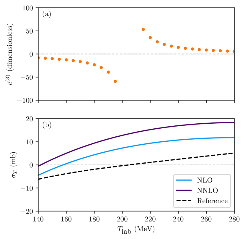
The LO predictions $y_{\text{th}}^{(0)}$ in $\Delta$-full $\chi$EFT are identical to the $\Delta$-less predictions and as such they are rather poor, as expected in Weinberg PC Carlsson et al. (2016); Yang et al. (2021). Thus, the $c^{(2)}$ expansion coefficients incur rather unnatural values. One could argue that a Bayesian approach, with a prior for the expansion parameters, should be able to properly handle such outliers. However, a (likely) deficient LO will conflict with our initial assumptions in Eq. (7). Instead of using the truncation error to absorb deficiencies rooted in the PC, we decided to neglect LO predictions in this paper. Thus, all training data consist of $c^{(3)}$ expansion coefficients only. Despite this limited amount of data, we expect the available coefficients to carry valuable information about the correlated truncation error and we proceed with a Bayesian $\mathcal{GP}$ model. For total and differential cross sections we set $y_{\text{ref}}$ to the predictions of the Idaho-N3LO(500) potential Entem and Machleidt (2003), which is almost the same as using $y_{\text{ref}}=y_{\text{exp}}$. We encounter a zero-crossing in $y_{\text{ref}}$ for $\sigma_{T}$. This leads to a discontinuity in the $c^{(3)}$ coefficients as a function of $T_{\text{lab}}$, see Fig. 1. Such small-scale structures are virtually impossible to faithfully represent using an infinitely smooth squared-exponential kernel. As there are only three experimental data points for this observable type we decided to exclude them from $\boldsymbol{\mathcal{D}}$. For polarization data we encounter an excess of small-scale structures when setting $y_{\text{ref}}$ to the predictions of Idaho-N3LO(500). Using $y_{\text{ref}}=0.5$ removes them entirely and we are spared further kernel design.

Figure 1: (a) Calculated expansion coefficients for $\sigma_{T}$. (b) The NLO, NNLO, and reference values from which the coefficients are calculated. Note the zero-crossing for the reference value at $T_{\textnormal{lab}}\approx 205$ MeV.

All training data are pruned for outliers using a three inter-quartiles threshold Svensson et al. (2022). In the end, all $c^{(3)}(\boldsymbol{x})$ coefficients are of natural order, and a vast majority of them pass the outlier filter. Operating with a $\mathcal{GP}$ allows us to incorporate known symmetry constraints on the polarization observables. Indeed, some polarizations are identically equal to zero at $\theta=0$ and/or $\theta=180$ degrees. We impose such boundary constraints by adding zero-valued expansion coefficients for the endpoint(s) of the angular direction to the training data. In a future application we will formally incorporate continuous boundary constraints in the $\mathcal{GP}$ Vernon et al. (2019).

We employ a bounded and uniform prior for the length scales $\vec{\ell}$ of the form

$$\textnormal{pr}(\ell_{\theta}|I)=\mathcal{U}(\epsilon,180)\,\,\text{degrees}$$ (27)

and

$$\textnormal{pr}(\ell_{T_{\text{lab}}}|I)=\mathcal{U}(\epsilon,290)\,\,\text{MeV},$$ (28)

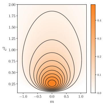
where $\epsilon=10^{-5}$ is introduced to avoid numerical issues in the optimization of the kernel. We place a conjugate normal-inverse-$\chi^{2}$ prior on the mean $m$ and variance $\bar{c}^{2}$ according to

$$\textnormal{pr}(m,\bar{c}^{2}|I)=\mathcal{N}\chi^{-2}(\eta_{0}=0,V_{0}=\frac{1}{2},\nu_{0}=1,\tau_{0}^{2}=1),$$ (29)

as shown in Fig. 2. This prior encodes our expectation on $\Delta$-full $\chi$EFT. We expect a natural $\bar{c}^{2}$ value, although the heavy tail in our prior allows for some unnaturalness, and expansion coefficients symmetrically distributed in the vicinity of zero.

Figure 2: The conjugate normal-inverse-$\chi^{2}$ prior $\textnormal{pr}(m,\bar{c}^{2}|I)$ for the $\mathcal{GP}$ hyperparameters.

The conjugacy of the $\mathcal{N}\chi^{-2}(m,\bar{c}^{2})$ prior implies that the posterior $\textnormal{pr}(m,\bar{c}^{2}|\vec{\ell},\boldsymbol{c}^{\star},\boldsymbol{x},I)$ is also a normal-inverse-$\chi^{2}$ pdf with updated parameters Melendez et al. (2019). The prior for the length-scale $\vec{\ell}$ is not conjugate, and to find the posterior MAP values $(\widehat{m},\widehat{\vec{\ell}},\widehat{\bar{c}^{2}})$ of

$$\begin{split}\textnormal{pr}(m,\vec{\ell},\bar{c}^{2}|\boldsymbol{c}^{\star},\boldsymbol{x}^{\star},I)\propto{}&\textnormal{pr}(\boldsymbol{c}^{\star}|m,\vec{\ell},\bar{c}^{2},\boldsymbol{x}^{\star},I)\times\\ {}&\textnormal{pr}(m,\bar{c}^{2}|I)\textnormal{pr}(\vec{\ell}|I)\end{split}$$ (30)

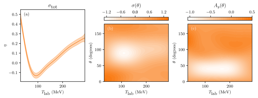
we use the numerical optimization routine L-BFGS-B Byrd et al. (1995) with multiple restarts. The resulting MAP estimates of the hyperparameters are listed in Table 1 and the mean $\mathcal{GP}$ predictions for expansion coefficients $c^{(3)}$ for three of the most abundant observable types are shown in Fig. 3.

The amount of training data is sufficient to make the posterior likelihood-dominated in most cases. We explored a prior with parameters $1/2\leq[\nu_{0},\nu_{0}\tau_{0}^{2}]\leq 3/2$ and we find that the inference is rather robust, as long as we allow for very small values $\bar{c}^{2}\gtrsim 0.2^{2}$. Indeed, a restrictive prior can bias the result for total cross sections, where the training data is one-dimensional.

Figure 3: Mean $\mathcal{GP}$ predictions $\eta$ for (dimensionless) expansion coefficients for (a) $\sigma_{\text{tot}}$ , (b) $\sigma(\theta)$, and (c) $A_{y}(\theta)$. The light colored band in (a) indicates a 95% credible interval.

IV.2 Validating the $\mathcal{GP}$ hyperparameters

We validate the $\mathcal{GP}$ for each observable type $y$ using a set of $N_{\text{val}}$ complementary validation data $\widetilde{\boldsymbol{c}}$. The validation data are generated by the same method as the training data, but with energies and angles shifted so that the validation values $\widetilde{\boldsymbol{x}}$ for the independent variable do not overlap with ones used during training. In addition to visual inspections, which are certainly useful, we follow Bastos and O’Hagan Bastos and O’Hagan (2009) and use also the Mahalanobis distance, pivoted Cholesky errors, and the credible interval as our diagnostics. These, and a few more, are thoroughly discussed in Ref. Melendez et al. (2019).

The (squared) Mahalanobis distance, $D^{2}_{\textnormal{MD}}$, is a multivariate analog to the sum of squared residuals. Here, it is computed as

$$D^{2}_{\textnormal{MD}}(\widetilde{\boldsymbol{c}},\eta(\widetilde{\boldsymbol{x}});\widetilde{\boldsymbol{\Sigma}}_{\mathcal{GP}})=[\widetilde{\boldsymbol{c}}-\eta(\widetilde{\boldsymbol{x}})]^{T}\widetilde{\boldsymbol{\Sigma}}_{\mathcal{GP}}^{-1}[\widetilde{\boldsymbol{c}}-\eta(\widetilde{\boldsymbol{x}})],$$ (31)

where $\eta(\widetilde{\boldsymbol{x}})$ denotes the $\mathcal{GP}$ output for the expansion coefficients at $\widetilde{\boldsymbol{x}}$ and

$$\widetilde{\boldsymbol{\Sigma}}_{\mathcal{GP}}=\widehat{\bar{c}^{2}}k(\widetilde{\boldsymbol{x}}^{\prime},\widetilde{\boldsymbol{x}};\widehat{\vec{\ell}}).$$ (32)

It is commonly used to quantify the deviation of a prediction compared to data in a correlated setting. Either too large or small values, compared to the reference $\chi^{2}$-distribution with $N_{\text{val}}$ degrees of freedom, point to a possible conflict between the $\mathcal{GP}$ prediction and the validation data. The Mahalanobis distance is a scalar measure and does not provide detailed insight about the possible tension with respect to the validation data.

Furthermore, it is instructive to make a point-by-point comparison of $\mathcal{GP}$ predictions and the validation data as a function of the independent variable. Such comparisons are not straightforward to interpret given the mutual correlation of the predictions. Therefore, we de-correlate and re-scale the prediction errors to independent unit variances using a Cholesky decomposition of the trained $\mathcal{GP}$ covariance matrix, i.e., $\widetilde{\boldsymbol{\Sigma}}_{\mathcal{GP}}=\boldsymbol{G}\boldsymbol{G}^{T}$ where $\boldsymbol{G}$ is a triangular standard deviation matrix. From this we define the Cholesky errors

$$\boldsymbol{D}_{G}=\boldsymbol{G}^{-1}[\widetilde{\boldsymbol{c}}-\eta(\widetilde{\boldsymbol{x}})].$$ (33)

To order the vector $\boldsymbol{D}_{G}$ in a meaningful way we pivot the decomposition in decreasing conditional predictive variances. One should not detect any pattern when plotting the pivoted $\boldsymbol{D}_{G}$ versus the index of the validation data. To reveal further information one can introduce a ratio scale also on the abscissa by plotting the pivoted Cholesky errors versus the conditional variances used for pivoting Al-Taweel (2018).

All but one of the $\mathcal{GP}$s readily pass our diagnostics, with $D^{2}_{\textnormal{MD}}$ landing within 95% credible intervals of the respective reference distributions. We see little-to-no structure in the pivoted Cholesky decompositions, and empirical coverages that roughly match the corresponding credible intervals. In addition, visual inspections indicate that the inferred hyperparameters are plausible. Naturally, incorporating expansion coefficients from other orders would provide a stronger test of our $\mathcal{GP}$ model. We only reject $\sigma_{T}$, and therefore also the three experimental data points. Neither $D^{2}_{\textnormal{MD}}$ nor the $\boldsymbol{D}_{G}$ exhibit significantly poor performance for this observable given our validation data. However, upon visual inspection of the $c^{(3)}$ curve for this observable, shown in Fig. 1, we find that it is discontinuous for $T_{\textnormal{lab}}\approx 205$ MeV because the reference value crosses zero at this point, leading to extremely large coefficients near the crossing point and an abrupt change in sign. Clearly, our $\mathcal{GP}$ model, based on a squared-exponential kernel, is ill-suited to handle this discontinuity, and the inferred length scale is strongly dependent on the chosen training data and will approach zero as we increase the number of training data. If it were not for the existence of an experimental data point in the vicinity of the problematic scattering energy we would have considered excluding only the problematic region. This example clearly shows that one should not blindly trust the diagnostics as they are conditioned on the chosen training and validation data.

IV.3 The structure of the correlated truncation error

Introducing a correlated truncation error reduces the number of independent directions in the data space. Indeed, two datum residing within one correlation length of the scattering energy or angle carries joint information. To quantify the impact of this we compute the effective dimension $n_{\text{eff}}$, per observable type $y$, using a measure Hill (1973); Giudice (2021) defined as $n_{\text{eff}}=\prod_{i=1}^{N_{d,y}}\kappa_{i}^{-\kappa_{i}}$, where $\kappa_{i}$ denotes a normalized eigenvalue $\kappa_{i}=\lambda_{i}/\text{tr}(\boldsymbol{C}_{y})$ of the respective correlation matrix. Here, $\boldsymbol{C}_{y}=\boldsymbol{S}_{y}^{-1}\boldsymbol{\Sigma}_{y}\boldsymbol{S}_{y}^{-1}$ and $\boldsymbol{S}_{y}=\sqrt{\text{diag}(\boldsymbol{\Sigma}_{y})}$ with $\boldsymbol{\Sigma}_{y}=\boldsymbol{\Sigma}_{\text{exp},y}+\boldsymbol{\Sigma}_{\text{th},y}$. We could equally well compute $n_{\text{eff}}$ for $\boldsymbol{\Sigma}_{y}$ directly. However, operating with the correlation matrix leads to the values $n_{\text{eff}}=1$ and $n_{\text{eff}}=N_{d,y}$ in the limits of having a full off-diagonal correlation and zero off-diagonal correlation, respectively. Consequently, we interpret $n_{\text{eff}}$ as the effective number of data, and note that the logarithm of $n_{\text{eff}}$ corresponds to the discrete Shannon entropy of the spectrum of the normalized eigenvalues ${\kappa_{i}}$.

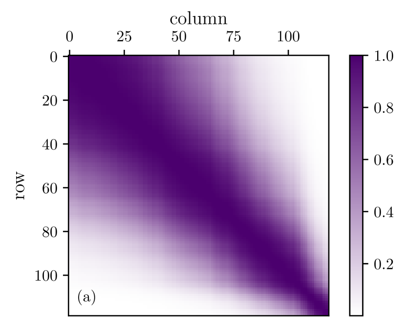
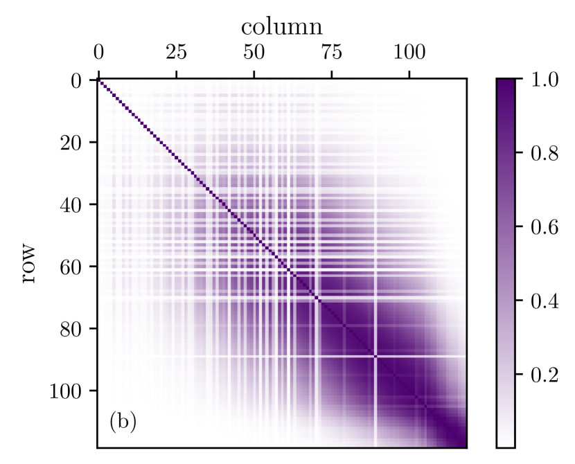
The resulting $n_{\text{eff}}$ values at NNLO are summarized in Table 1. They show that the correlations reduce the number of effective data from 2087 to 838, which is still plentiful. The main reason for the relatively weak impact of the correlated truncation error is the dominance of the experimental variances along the diagonal of the covariance matrix $\boldsymbol{\Sigma}$. Indeed, for the correlation matrices of the $\mathcal{GP}$ kernel for EFT truncation errors alone we find $n_{\text{eff}}\approx 5-10$. In Fig. 4 we show correlation matrices for the total cross section $\boldsymbol{C}_{\sigma_{\text{tot}}}$, with and without the experimental covariance matrix accounted for. The diagonal dominance of the experimental errors is clearly visible. This dominance weakens for higher energies (higher indices in the figure) as the truncation error increases with the scattering energy $T_{\text{lab}}$.

Figure 4: Correlation matrices based on the NNLO covariance matrix $\boldsymbol{\Sigma}_{\sigma_{\text{tot}}}$ of the 119 $\sigma_{\text{tot}}$ data. In panels (a) and (b) we exclude and include, respectively, the experimental variances $\boldsymbol{\Sigma}_{\text{exp},\sigma_{\text{tot}}}$. The data is sorted by energy in increasing order.

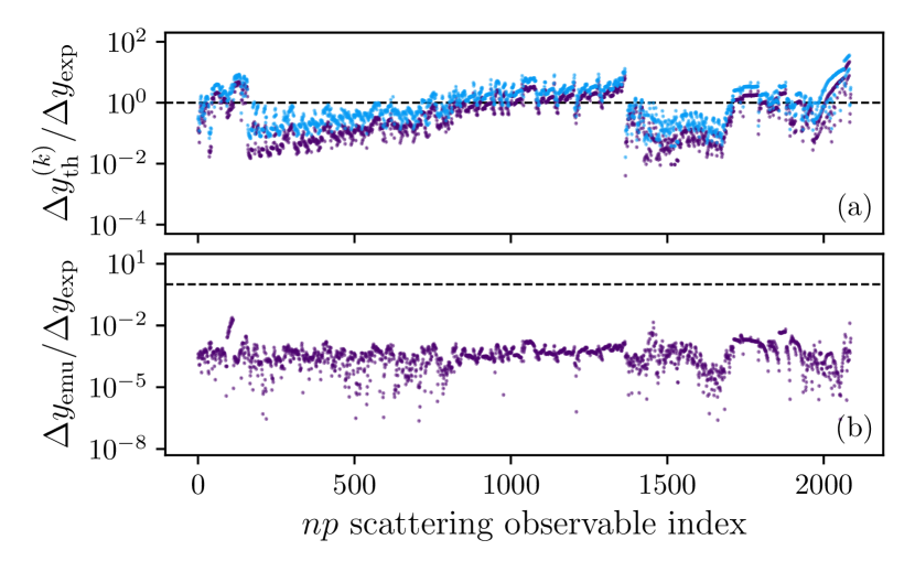
At NLO, where the truncation error is greater by one chiral order $Q$, the corresponding $n_{\text{eff}}$ values are typically a factor two smaller as the correlations of the truncation error become relatively more important. The total number of effective data is 488. In Fig. 5(a) we compare the 68% credible interval $\Delta y_{\text{th}}^{(k)}$ of the EFT truncation error at NLO and NNLO with the experimental errors $\Delta y_{\text{exp}}$ for all data.

The EFT truncation error, and its correlations, is expected to be more important for inferences conditioned on very precise $pp$ data. To estimate this effect, we inspected the $pp$ $A_{y}(\theta)$ data set closer. With $T_{\text{lab}}\in[30,290]$ MeV there are 496 data-points, which is almost the same as in the $np$ sector. Reducing the experimental variances of the $np$ $A_{y}(\theta)$ data, to mimic the average level of $pp$ variances, we observe $n_{\text{eff}}=138$ and 76 at NNLO and NLO, respectively. For other observable types, like $\sigma(\theta)$, the average $pp$ variance is greater than the average $np$ variance, and the opposite effect is likely observed. Note that the distribution of $np$ and $pp$ measurement energies and angles differ and we do not account for this in our estimate.

V Emulating $np$ scattering cross sections

We use an EC-based method König et al. (2020) to construct accurate and efficient emulators for $np$ scattering observables. Operating with emulators, instead of the exact simulators, help reduce the computational cost of evaluating the likelihood. As an added bonus, once the emulators are trained they are straightforward to distribute in the scientific community.

We use Newton’s functional formulation of on-shell $np$ $T$-matrix elements for setting up the emulators Melendez et al. (2021). Technically, this leads to one emulator per $np$ partial-wave and unique scattering energy in the database $\boldsymbol{\mathcal{D}}$ (Table 1). Truncating the partial-wave expansion at a maximum $np$ angular-momentum quantum number $J=30$ leads to 182 partial waves. With $N_{T_{\text{lab}}}=177$ energies in $\boldsymbol{\mathcal{D}}$ we end up with $32\,214$ $T$-matrix emulators per chiral order. The training values for the LECs are drawn according to a latin hypercube design in a sufficiently wide interval $[-4,+4]$ (see Sec. III.1 for units). To simplify the setup, we employ the same training protocol for all emulators and find it sufficient to use 7 (8) training points at NLO ( NNLO). As there are at most $3$ ($7$) relevant LECs acting per partial wave, this approach leads to very accurate emulation of all relevant scattering observables. We estimate that emulator errors $\Delta y_{\text{emu}}$ are at least 10, and typically 1000, times smaller than experimental errors. This is quantified using the difference between emulated and exact results for all $np$ observables in $\boldsymbol{\mathcal{D}}$ at ten different sets of LEC values following randomized latin hypercube designs within the training intervals specified above. In Fig. 5(b) we show the ratio $\Delta y_{\text{emu}}/\Delta y_{\text{exp}}$ at NNLO for a random set of LEC values. This is virtually identical to the NLO result. We conclude that the emulator errors are sufficiently small to neglect them in our inferences. In the following we refer to the collection of all amplitude-emulators, per chiral order, as the emulator for scattering observables $y$.

Figure 5: The EFT truncation and EC emulator errors compared to experimental errors for all considered $np$ scattering data. (a) The standard deviations of the EFT truncation errors at NLO and NNLO. (b) The NNLO EC emulator errors ($\Delta y_{\textnormal{emu}}$). Colors as in Fig. 1. In both panels we divide by the the experimental $1\sigma$ errors ($\Delta y_{\textnormal{exp}}$) and the horizontal dashed lines indicate a ratio of one.

VI Sampling posterior distributions

We sample the LEC posteriors $\textnormal{pr}(\vec{\alpha}|\boldsymbol{\mathcal{D}},I)$ at NLO and NNLO using HMC, an advanced MCMC algorithm suitable for high-dimensional sampling problems. We have detailed the use and performance of HMC in a previous paper Svensson et al. (2022) and further improved its performance in Ref. Svensson et al. (2023). Here, we employ the same sampling strategy as in the latter paper. HMC needs tuning in order to perform well, and in particular a good so-called mass matrix is needed. The mass matrix should be a decent approximation to the inverse of the parameter covariance matrix. We extract such an approximation by maximizing the posterior through the standard BFGS algorithm Broyden (1970); Fletcher (1970); Goldfarb (1970); Shanno (1970).

HMC requires gradients of the (logarithm of the) posterior with respect to the sampled parameters. The underlying linearity of the emulators furnish easy access to derivatives of $T$-matrix amplitudes with respect to the LECs. However, we employ the automatic differentiation (AD) and just-in-time compilation (JIT) tools for Python in the Google JAX Bradbury et al. (2018) library to compute the required gradients and boost the execution speed of our Python code; it takes on the order of one second to evaluate the entire data likelihood, including derivatives. We opted for this approach due to its simplicity and speed. It also enables straightforward computation of derivatives of the posterior with respect to parameters other than the LECs, such as $\mathcal{GP}$ hyperparameters. A threaded C-code implementation would likely be more efficient, but not pivotal for the present applications.

We diagnose the convergence of the MCMC chains using a criterion based on the integrated autocorrelation time $\tau_{\textnormal{int}}$ Sokal (1997). This is a measure of the autocorrelation between MCMC samples, and it tends to be underestimated for short MCMC chains. In line with Ref. Svensson et al. (2022) we therefore declare convergence when (a) the estimation of $\tau_{\textnormal{int}}$ has stabilized, and (b) when $N\geq 50\tau_{\textnormal{int}}$, where $N$ is the length of the MCMC chain. All our chains readily pass this test. Like other MCMC convergence tests, the $\tau_{\textnormal{int}}$ criterion may falsely declare convergence, e.g., if the posterior is multimodal; we therefore search for local optima using BFGS optimization initialized at random positions. We have not detected signs of multi-modality and are confident that our chains are converged.

VI.1 LEC posteriors

In a first step we compare the LEC posteriors obtained with correlated and uncorrelated EFT truncation errors. In the uncorrelated limit we determined $\bar{c}^{2}$ from the root-mean-square value of the NLO- NNLO expansion coefficients for the $\sigma_{\text{tot}},\sigma(\theta),A_{y}(\theta)$ observables, i.e., omitting the LO contribution and discarding outliers. We employed the same grids of scattering energies and angles as in the training of the correlated $\mathcal{GP}$ model for these observables, see Sec. IV.1. This leads to a fixed $\bar{c}^{2}=0.42^{2}$.

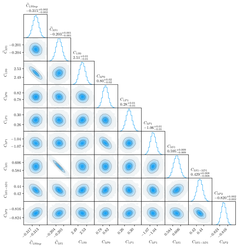
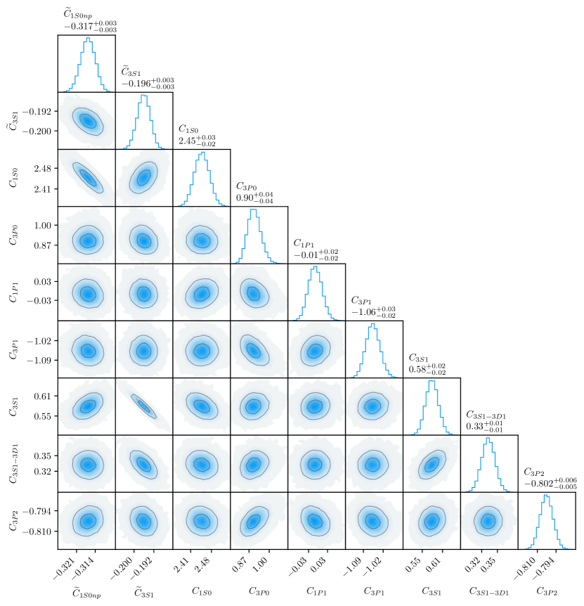
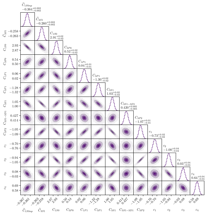
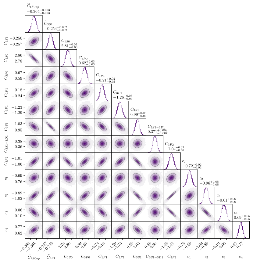
We find that the introduction of a finite correlation length in the EFT truncation error does not affect the marginal LEC posteriors much, see Figs. 8, 9, 10, 11 in Appendix A. However, there are some differences and similarities worth commenting on. Most noticeably, the marginal posteriors for all LECs are approximately twice as wide when including a correlated truncation error. This is consistent with the observed reduction in the effective number of data. Other than that, the posterior correlation structure remains the same and the respective locations of the modes are largely the same, except for a significant shift in the value of the $C_{3S1-3D1}$ contact and that the $C_{1P1}$ contact LEC becomes (almost) consistent with zero in the correlated (uncorrelated) limit at NLO ( NNLO). At NNLO  the MAP value for the subleading $\pi N$ LECs are substantially shifted with respect to the mean of their prior values in Eq. (10). This result does not change when neglecting a correlated truncation error. In the case of a correlated truncation error we obtain a MAP value for the $\pi N$ LECs

$$\widehat{\vec{\alpha}}_{\pi N}=[-0.72(2),-0.96(5),-0.01(6),0.69(5)]\,\text{GeV}^{-1},$$ (34)

with 68% credible intervals indicated by error bars in parentheses. The squared Mahalanobis distance of this point with respect to the mean and covariance of the prior is $D^{2}_{\textnormal{MD}}(\widehat{\vec{\alpha}}_{\pi N},\vec{\mu}_{\pi N};\Sigma_{\pi N})=9.65$, which is just far enough for the posterior MAP value to be outside 95% of the prior probability mass. This can be cast in terms of a $p$-value (0.047) and traditional significance testing, which would lead us to reject the correctness of the Roy-Steiner prior (null hypothesis) on the 5% significance level. However, we are inclined to place doubt on our model for the truncation error and in particular its variance. As a side remark, the $D^{2}_{\textnormal{MD}}$-values for the MAP values of the $\pi N$ LEC posteriors for $\Delta$-less NNLO Svensson et al. (2022), and the next order N3LO Svensson et al. (2023), inferred using an uncorrelated truncation error, are even greater and again point to significant tension between the respective LECs inferred using $NN$ data and $\pi N$ data.

We suspect that the truncation error is underestimated since the NLO- NNLO shift in the $\Delta$-full theory is on the smaller side, which is not too surprising as the inclusion of the $\Delta$-isobar pulls down higher-order contributions in the $\Delta$-less theory. Also, we cannot rule out that the contributions at $\Delta$-full N3LO are substantial owing to the introduction of a rich fourth-order contact potential. To shed some light on the possible underestimation of $\bar{c}^{2}$ we sampled the joint posterior $\textnormal{pr}(\vec{\alpha},\bar{c}^{2}|\boldsymbol{\mathcal{D}},I)$ in the uncorrelated limit of the truncation error. For this, we employed the same LEC prior as defined in Sec. III.1, and assume the same $\bar{c}^{2}$ for all observable types. For the latter parameter we employ an inverse-$\chi^{2}$ prior with $\nu=23.75$ and $\tau^{2}=0.19$, as obtained via conjugacy of an inverse$-\chi^{2}$ (hyper)prior with $\nu_{0}=\tau_{0}^{2}=1$ updated using training data from expansion coefficients $c^{(3)}$ for $\sigma(\theta),A_{y}(\theta),\sigma_{\text{tot}}$ on the same grid of $\theta$ and $T_{\text{lab}}$ values as used when inferring the $\mathcal{GP}$ model parameters for the correlated truncation error. This prior is sharply peaked at $\bar{c}^{2}\approx 0.45^{2}$. The marginal LEC values from the $\textnormal{pr}(\vec{\alpha},\bar{c}^{2}|\boldsymbol{\mathcal{D}},I)$ posterior are not noticeably different from before. However, the posterior mode for $\bar{c}^{2}$ is $0.96(5)$ and $3.5(2)$ at NLO, and NNLO, respectively, with 68% credible intervals indicated in parenthesis. Clearly, conditioning on $\boldsymbol{\mathcal{D}}$ has a significant impact and increases the EFT truncation error.

VI.2 Posterior predictive distributions

In this section we present posterior predictive distributions (PPDs) for, preferably unseen, scattering observables $y^{\star}=y(\vec{x}^{\star})$ at some value(s) $\vec{x}^{\star}$ for the independent variable. The predictions are marginalized over $\vec{\alpha}$ using the relevant LEC posteriors at chiral order $k$, i.e.,

$$\textnormal{pr}(y^{\star}|\boldsymbol{\mathcal{D}},\vec{x}^{\star},I)=\int d\vec{\alpha}\,\,\textnormal{pr}(y^{\star}|\vec{\alpha},\vec{x}^{\star},I)\textnormal{pr}(\vec{\alpha}|\boldsymbol{\mathcal{D}},I),$$ (35)

where we subsume $k$ and assumptions about the truncation error in $I$. Our predictions account for a normally distributed truncation error via

$$\textnormal{pr}(y^{\star}|\vec{\alpha},\vec{x}^{\star}I)=\mathcal{N}(y_{\text{th}}^{(k)}(\vec{\alpha};\vec{x}^{\star})+M^{(k)}_{y},\Sigma^{(k)}_{\text{th},y}).$$ (36)

In the correlated case, the mean $M_{y}^{(k)}$ and covariance $\Sigma^{(k)}_{\text{th},y}$ are obtained from a $\mathcal{GP}$ with MAP values $\widehat{\ell_{\theta}},\widehat{\ell_{T_{\text{lab}}}},\widehat{\bar{c}^{2}}$ according to the values listed in Table 1.

As a model check we first inspect the PPD for some of the seen data, i.e., the data already in $\boldsymbol{\mathcal{D}}$. In Fig. 6 we show 500 draws from the PPDs $\textnormal{pr}(A_{y}(\theta)|\boldsymbol{\mathcal{D}},\boldsymbol{x},I)$ for the vector polarization at NLO with $T_{\text{lab}}=40$ MeV and $T_{\text{lab}}=140$ MeV.

Figure 6: 500 draws from the NLO PPDs for $A_{y}(\theta)$ at $T_{\text{lab}}=40$ MeV and $T_{\text{lab}}=140$ MeV using a correlated truncation error. The experimental data at $40$ MeV and $140$ MeV are from Refs. Wilczynski et al. (1984); Langsford et al. (1965) and Stafford et al. (1957), respectively.

Figure 7: 500 draws from the PPDs for unseen data for: (a) $\sigma(\theta)$ at NNLO and $T_{\text{lab}}=319$ MeV with a correlated error, and experimental data from Ref. Keeler et al. (1982). (b) Same as (a) but with an uncorrelated error. (c) $A_{y}(\theta)$ at NNLO and $T_{\text{lab}}=350$ MeV with a correlated error, and experimental data from Ref. Siegel et al. (1956). (d) Same as (c) but with a correlated error. (e) $\sigma_{\text{tot}}$ at NLO and $T_{\text{lab}}=30$-$350$ MeV (see Ref. Pérez et al. (2013) for references to the experimental data).

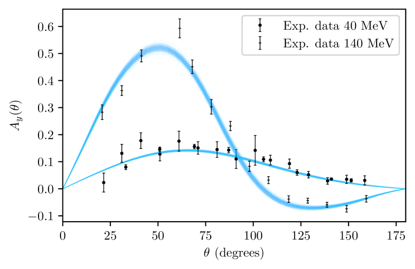
The model calculations were performed using EC emulators trained as above. The observed correlation length, $\widehat{\ell_{\theta}}=32$ degrees, is reasonable, and we hit most of the data within the theory uncertainty. Due to the symmetries of the strong interaction we must have $A_{y}(\theta=0)=A_{y}(\theta=180)=0$. As we incorporated this type of constraint during the training the $\mathcal{GP}$, the predictive variance indeed goes to zero for $\theta=0,180$. Given the rather long correlation lengths, the variance constraints at the angular endpoints appears to propagate to the interior to further suppress the truncation error. We have not studied the empirical coverage of the truncation error as we expect it to extrapolate rather poorly to unseen data at higher energies.

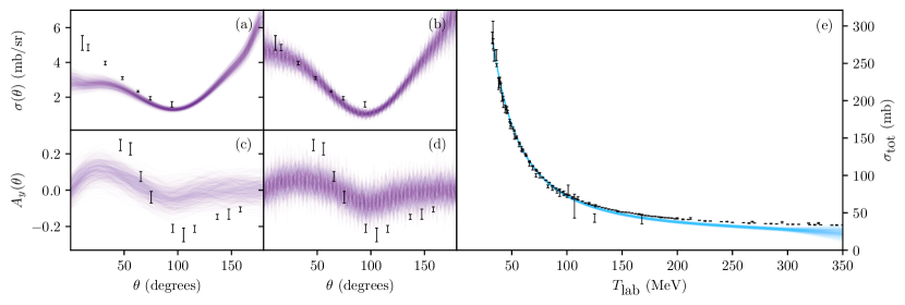
In Fig. 7 we quantify PPDs for unseen data and compare predictions based on correlated and uncorrelated truncation errors. We have drawn 500 samples from the PPDs for the differential cross section $\sigma(\theta)$ at $T_{\text{lab}}=319$ MeV, the vector polarization $A_{y}(\theta)$ at $T_{\text{lab}}=350$ MeV, and the total cross section $\sigma_{\text{tot}}$ for $T_{\text{lab}}=30-350$ MeV, where the latter is at NLO and the former two at NNLO using correlated as well as uncorrelated truncation errors.

The smoothing effect of the correlated truncation error is clearly visible in panels (a) and (c). For $\sigma(\theta)$, in panels (a) and (b), the predictions in the low-$\theta$ region fare significantly worse when including correlations. We speculate that this is connected to the reduced weight of high-energy $np$ data residing within one correlation length of the truncation error. In panels (c) and (d) we compare $A_{y}(\theta)$ predictions at NNLO. Besides overall similarities, the predictive variance of $A_{y}(\theta$) is finite at the edges even when we include a correlated truncation error for which we have imposed the relevant symmetry constraints. However, at $T_{\text{lab}}=350$ we are approximately one correlation length away from the training point where the constraint was imposed, and its effect has deteriorated. Finally, the PPD for the total cross section in panel (e) underestimates the experimental data for $T_{\text{lab}}>100$ MeV, and the correlated truncation error appears to be somewhat too small as well.

VII Summary and Outlook

We quantified a correlated truncation error for $\Delta$-full $\chi$EFT predictions of $np$ scattering observables at NLO and NNLO. The correlation structure was modeled using a $\mathcal{GP}$ with a squared-exponential kernel, and the resulting MAP values for the correlation lengths in the scattering energy and angle directions are in the ranges of 40–120 MeV and 25–45 degrees, respectively, for the 17 different observable types in the set of $np$ scattering data that we consider. These are significant correlation lengths that, in principle, could reduce the effective number of independent $np$ data in the likelihood by two orders of magnitude and therefore strongly impact the LEC inference. However, other than doubled widths of the univariate marginal posteriors for all LECs we find that the introduction of a correlated EFT truncation error does not change the structure of the LEC posteriors by much. This is explained well by the relatively small marginal variances of the truncation errors that we quantify in this paper. Indeed, we found effective dimensions of the data likelihood that were approximately 1/8 and 1/4 of the length of the experimental $np$ database, at NLO and NNLO respectively.

The marginal variance of the uncorrelated truncation error increases up to four times when jointly sampling it with the LEC values. Thus, future inferences should attempt to marginalize predictions over the hyperparameters of the $\mathcal{GP}$ model and if possible also the breakdown scale, or the expansion parameter $Q$. For this, the HMC algorithm with AD should provide the necessary leverage to enable sampling of a posterior with, at least, doubled dimensionality. There is most likely useful information to learn about the truncation error from theoretical predictions at N3LO in $\Delta$-full $\chi$EFT. Adding more chiral orders in the analysis of the truncation error might reveal challenging structures in the order-by-order data that call for more sophisticated $\mathcal{GP}$-kernel design than we employ in this paper.

It will be interesting in future studies to explore the performance of the inferred interactions in predictions of many-nucleon observables. The general ab initio modeling capabilities of $\Delta$-full chiral interactions at NNLO were studied recently in Refs. Hu et al. (2022); Jiang et al. (2022a, b). These papers targeted, in particular, predictions for heavy nuclei up to ²⁰⁸Pb and infinite nuclear matter. A common strategy was to first use history matching to identify interaction parameterizations that give acceptable model predictions for a suite of low-energy nuclear observables. Energies and radii of light nuclei, as well as selected $np$ phase shifts, were included sequentially in an implausibility measure that led to the removal of large regions of the LEC parameter space. Although a lower regulator-cutoff $\Lambda=394$ MeV was used in the history-matching analyses, it is still interesting to compare the identified regions with the parameter posterior PDF inferred in this paper. First, we find that the posterior mode from this paper projected on $c_{2,3,4}$ is situated just outside the non-implausible range. That is not surprising since the Roy-Steiner prior was employed without updates throughout history matching. Furthermore, the mode is located at the upper end of the non-implausible range in the $C_{1S0}$ direction and at the lower edges of the $C_{1P1}$ and $C_{3P2}$ ranges. The significance and origin of this tension should be explored in a joint analysis of $NN$, few-, and many-nucleon observables.

The scattering emulators and HMC sampling presented here can be combined with history matching and reduced-basis methods for many-body observables to enable a joint analysis of chiral interactions. Such studies, however, will rely on an improved understanding of correlated EFT truncation errors and soft momentum scales in finite nuclei.

Appendix A LEC posteriors PDFs

In this appendix we show the LEC posterior PDFs for the values of the LECs in $\Delta$-full $\chi$EFT up to NNLO, conditioned on $np$ scattering data with $30\leq T_{\text{lab}}\leq 290$ MeV and a truncation error in the correlated and uncorrelated limits.

Figure 8: Posterior PDF of the values for the LECs at NLO inferred using an EFT truncation error in the uncorrelated limit. The inner (outer) gray contour line encloses 39% (86%) of the probability mass. The dot-dashed vertical lines indicate a 68% credibility interval in the univariate marginals. See main text for units and conventions.

Figure 9: Posterior PDF of the values for the LECs at NLO inferred using a correlated model for the EFT truncation error. See Fig. 8 for figure notation.

Figure 10: Posterior PDF of the values for the LECs at NNLO inferred using an EFT truncation error in the uncorrelated limit. See Fig. 8 for figure notation.

Figure 11: Posterior PDF of the values for the LECs at NNLO inferred using a correlated model for the EFT truncation error. See Fig. 8 for figure notation.