A hard look at the X-ray spectral variability of NGC 7582

Abstract

NGC 7582 ($z=0.005264$; $D=22.5$ Mpc) is a highly variable, changing-look AGN. In this work, we explore the X-ray properties of this source using XMM-Newton and NuSTAR archival observations in the 3-40 keV range, from 2001 to 2016. NGC 7582 exhibits a long-term variability between observations but also a short-term variability in two observations that has not been studied before. To study the variability, we perform a time-resolved spectral analysis using a phenomenological model and a physically-motivated model (uxclumpy). The spectral fitting is achieved using a nested sampling Monte Carlo method. uxclumpy enables testing various geometries of the absorber that may fit AGN spectra. We find that the best model is composed of a fully covering clumpy absorber. From this geometry, we estimate the velocity, size and distance of the clumps. The column density of the absorber in the line of sight varies from Compton-thin to Compton-thick between observations. Variability over the timescale of a few tens of kilo-seconds is also observed within two observations. The obscuring clouds are consistent with being located at a distance not larger than $0.6$ pc, moving with a transverse velocity exceeding $\sim 700$  km s^-1. We could put only a lower limit on the size of the obscuring cloud being larger than $10^{13}~{}$cm. Given the sparsity of the observations, and the limited exposure time per observation available, we cannot determine the exact structure of the obscuring clouds. The results are broadly consistent with comet-like obscuring clouds or spherical clouds with a non-uniform density profile.

1 Introduction

Active Galactic Nuclei (AGN) are energetic sources exhibiting a high bolometric luminosity, located at galactic centres. They are powered by the accretion of matter onto a supermassive black hole with $M_{\mathrm{BH}}\gtrsim 10^{6}~{}\mathrm{M}_{\odot}$ via an inspiraling disc, known as the accretion disc. This disc is thought to be typically optically thick and geometrically thin (Shakura & Sunyaev, 1973), emitting thermal radiation in the optical and ultraviolet range. In addition, a strong X-ray emission is observed in AGN and attributed to the up-scattering of disc photons by electrons in a hot plasma called the corona (Haardt & Maraschi, 1993).

Using optical/UV spectra, active galaxies can be classified as: Type-1 that show narrow (Full Width at Half Maximum, FWHM, less than $1000$ km s^-1) and broad emission lines ($\rm FWHM>1000$ km s^-1) and Type-2 that show narrow emission lines only. Optical lines are Doppler-broadened closer to the black hole in the eponymous region, Broad Line Region (BLR), in opposition to the Narrow Line Region (NLR) which is thought to be located farther from the black hole, where narrow lines are produced. The BLR is typically located at a distance less than one parsec (see Kaspi et al., 2005) whereas the NLR can extend from dozens to hundreds of parsecs (Mor & Netzer, 2012).

The unified model of AGN (Antonucci & Miller, 1985; Antonucci, 1993; Urry & Padovani, 1995) explained the variety in AGN by the difference in viewing angle at which we observe the source. In this model, Type-1 sources are observed face-on providing a direct look at the central engine. Instead, Type-2 sources are observed with a higher inclination where obscuration of the central engine and BLR clouds by the parsec-scale dusty torus becomes more important. X-ray observations can be used to estimate the equivalent hydrogen column density ($N_{\rm H}$) of the obscurer which can be classified as Compton-thin or Compton-thick if $N_{\rm H}$ is smaller or larger than $\sim 1.5\times 10^{24}\,$ cm^-2, respectively. However, many sources, can change from Type-1 to Type-2 and vice versa between observations, associated with the appearance/vanishing of broad optical lines (see e.g., LaMassa et al., 2015). Ricci & Trakhtenbrot (2022) referred to these objects as Changing accretion-state (CS) AGN. Whereas, AGN changing from Compton-thick to Compton-thin and vice versa in X-ray observations are referred to as Changing-obscuration (CO) AGN. The proposed interpretations for CO-AGN transitions are the passage of obscuring material in the BLR across our line of sight or absorption by ionised material. In the case of CS-AGN, the obscuration of the source is ruled out in favour of disk instabilities or stellar tidal disruption events (see e.g., Ricci et al., 2021).

In this work, we study NGC 7582, a nearby ($z=0.005264$, $D=22.5$ Mpc) Seyfert 2 galaxy with a changing-look behaviour. Wold et al. (2006) estimated the black hole mass to be $M_{\mathrm{BH}}={5.5^{+3.2}_{-2.3}\times 10^{7}\,\mathrm{M}_{\odot}}$ by modelling the gas dynamics in the mid-infrared. This source has been observed in X-rays in several occasions since the late 70’s. Ward et al. (1978) associated the X-ray source 2A 2315-428, detected with the Ariel 5 survey, with the galaxy NGC 7582. These observations revealed the presence of a flux variability by a factor of 4 over 60 days. Mushotzky (1982) analysed three HEAO-1 observations. The source revealed short timescale variability with a flare where the count-rate doubled over a timescale of $1.5~{}$days. Using a Ginga observation, Warwick et al. (1993) established the presence of a large intrinsic column density of absorbing material in the nuclear region. Later on, Aretxaga et al. (1999) reported on a broadening of the H$\alpha$ line, which involved a transition from Type-2 to Type-1, which labelled NGC 7582 as a changing-look AGN. XMM-Newton observed the source for the first time in 2001, catching the source in a low-flux state. Dewangan & Griffiths (2005) and Awaki et al. (2006) analysed this observation, and confirmed the detection of a clear iron line at $\sim 6.4$ keV. Bianchi et al. (2007) mapped the nuclear region using Chandra and the Hubble Space Telescope. The authors report the presence of a dust lane in the optical, and concluded that soft X-ray emission (below $3$ keV) corresponds to the region where the dust lane is thinner. Piconcelli et al. (2007) analysed XMM-Newton data from observations of 2001 and 2005. They proposed a model for the absorption that consists of a thin neutral absorber and an inner thick neutral absorber composed of clouds where X-ray photons are reflected via Compton scattering. Bianchi et al. (2009) analysed four Suzaku and one XMM-Newton observation, taking place in 2007, which were compared to the previous XMM-Newton observations of 2001 and 2005. The authors observed an increase in the column density of the inner thick absorber during the Suzaku campaign. They invoked a third, Compton-thin, absorber in their model, that is associated with the dust lanes outside of the torus observed with Chandra and HST. The authors ascribed the observed variability to absorbing material drifting in the BLR. Later on, Rivers et al. (2015) studied two NuSTAR observations and one Swift observation, taken in 2012. They modelled the absorption with a thick patchy torus and a thin full-covering absorber. They found the most plausible scenario explaining the variability to be the obscuration of the nucleus. More recently, Braito et al. (2017) analysed two Chandra HETG observations performed in 2014, and a Suzaku one performed in 2007. They found a constant reflection component associated with the inner edge of the clumpy torus. A highly ionised absorber was also detected in the Chandra spectra.

In this work, we present a comprehensive analysis of all the archival XMM-Newton and NuSTAR observations of NGC 7582 with the aim of explaining the short- and long-term behaviour of the source. The paper is organised as follows. In Section 2, we describe the observations analysed in this work and the corresponding data reduction. In Section 3 we present the tools and models used for the X-ray spectral analysis. Our results are presented in Section 4 and discussed in Section 5. Conclusions are drawn in Section 6.

2 Observations and data reduction

NGC 7582 was observed five times by XMM-Newton between 2001 and 2018 and three times by NuSTAR between 2012 and 2016, including a simultaneous observation between XMM-Newton and NuSTAR in 2016. We use all of the archival XMM-Newton and NuSTAR observations, except the XMM-Newton observation of 2018. The source was off-axis by more than 10 arcmin, falling on a bad pixel column. The data from this observation could not be used as they suffered from calibration issues in energy and normalisation. We present in Table 1 the observations used in this work and the associated net exposure times.

Table 1: Observations used in this work and their associated exposure time after removing the bad time intervals. For XMM-Newton the exposures are given for the EPIC instruments pn, MOS1 and MOS2, and for NuSTAR the net exposures are given for FPMA and FPMB.

Observation ID	Observatory	Date	Exposure (ks)
0112310201	XMM-Newton	25 May 2001	17.5 / 22.4 / 22.4
0204610101	XMM-Newton	29 Apr 2005	61.8 / 75.4 / 76.3
0405380701	XMM-Newton	30 Apr 2007	1.9 / 8.6 / 8.6
60061318002	NuSTAR	31 Aug 2012	16.5 / 16.4
60061318004	NuSTAR	14 Sept 2012	14.6 / 14.6
0782720301	XMM-Newton	28 Apr 2016	42 / 98.5 / 98.5
60201003002	NuSTAR	28 Apr 2016	48.5 / 48.3

2.1 XMM-Newton

XMM-Newton data from the EPIC instruments pn (Strüder et al., 2001) and MOS (Turner et al., 2001) were reduced using the Science Analysis System (SAS 20.0; Gabriel et al., 2004). We used the recent empirical calibration to improve the spectral agreement between XMM-Newton and NuSTAR above 3 keV. We filtered periods of high background flaring activity in the event lists with the recommended rate threshold of $0.4$ $\rm Count~{}s^{-1}$ for the EPIC-pn and $0.35$ $\rm Count~{}s^{-1}$ for the EPIC-MOS detectors. The source was extracted from a circular region of $30~{}^{\prime\prime}$ and the background was extracted from a circular source-free region of the same chip with a radius of $60~{}^{\prime\prime}$. Source and background light-curves were extracted in the soft energy band 0.5-3 keV and in the hard energy band 3-10 keV using the task evselect. A binning of 1 ks was chosen for all observations. XMM-Newton source and background spectra are extracted with the task evselect. The Ancillary Response File (ARF) is generated with arfgen and the Redistribution Matrix File (RMF) is produced with rmfgen. The spectral files are grouped with specgroup to have a minimum signal-to-noise ratio of five and ensuring that the width of the bins is not narrower than one-third of the energy resolution.

Figure 1: Light-curves of the XMM-Newton and NuSTAR observations in the 0.5-3 keV (top panel) energy band and 3-10 keV (bottom panel) energy band for the EPIC-pn (dark blue circles), EPIC-MOS1 (green squares), EPIC-MOS2 (light blue diamonds), FPMA (yellow hexagons) and FPMB (magenta pentagons). The count-rates are normalised to the count-rates of the observation of 2016. The dashed vertical lines show the chosen slices for the extraction of spectra, the slices are indicated by circled numbers ①, ②, ③, …

2.2 NuSTAR

NuSTAR (Harrison et al., 2013) data were reduced using the NUSTARDAS 2.1.1 package part of HEAsoft 6.29 and the calibration files of CALDB 20210210. The task nupipeline was used to produce calibrated data as well as filtered event lists. Source and background regions were selected as circular regions with a radius of 80″ on both instruments FPMA and FPMB. Source and background light-curves were extracted for the 3-10 keV and 10-40 keV energy bands using the task nuproducts. We use NuSTAR data only up to 40 keV as they are background dominated above this energy. To keep consistency with the XMM-Newton observations a temporal binning of 1 ks was chosen. Source and background spectra, ARF, and RMF, are extracted using the task nuproducts and grouped to at least 30 counts per energy bin.

Figure 2: Light-curves of NuSTAR observations in the 10-40 keV band for the detectors FPMA (yellow hexagons) and FPMB (magenta pentagons).

Table 2: Mean count-rate (Counts $\mathrm{s}^{-1}$) of XMM-Newton and NuSTAR observations in the 0.5-3 keV and 3-10 keV band.

	Mean count-rate (Counts $\mathrm{s}^{-1}$)
	0.5-3 keV 3-10 keV			3-10 keV
Date	pn	MOS1	MOS2	FPMA	FPMB
2001-05	$0.282$ $0.276$	$0.0792$ $0.0779$	$0.0887$ $0.0828$	-	-
2005-04	$0.274$ $0.159$	$0.0779$ $0.0428$	$0.0828$ $0.0461$	-	-
2007-04	$0.319$ $0.462$	$0.0946$ $0.134$	$0.931$ $0.140$	-	-
2012-08	-	-	-	$0.193$	$0.194$
2012-09	-	-	-	$0.127$	$0.132$
2016-04	$0.285$ $0.521$	$0.0784$ $0.154$	$0.0787$ $0.169$	$0.377$	$0.386$

2.3 Short-term and long-term Variability

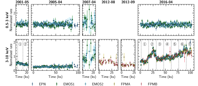
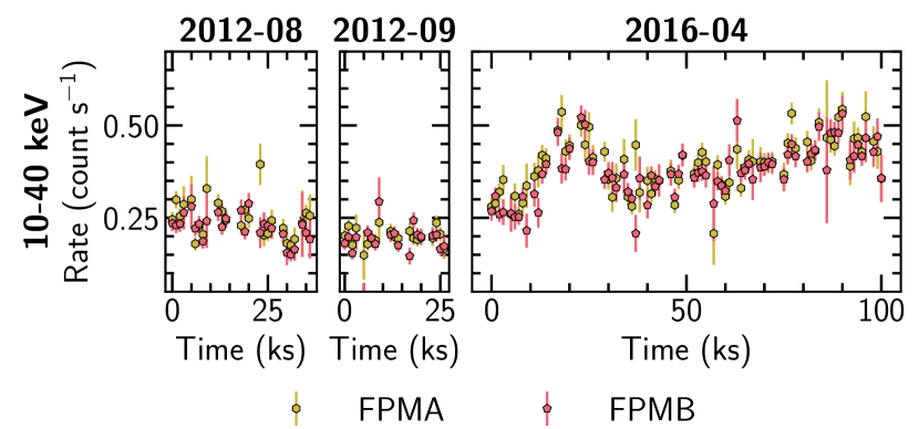
The light-curves of the XMM-Newton and NuSTAR observations are shown in Figure 1, normalised to the mean count-rates of the observation of 2016. The mean count-rates of the observations are given in Table 2. The light-curves in the 0.5-3 keV range do not show any intra-/inter-observation variations. However, the variability is larger in the 3-10 keV range. The light-curve of the observation of 2001 appears to be decreasing towards the end of the observation. No variability is observed in the observation of 2005, which has the lowest count-rate among the analysed observations. For the observation of 2007, as the light-curve does not have sufficient data points, we cannot derive any conclusions on its variability. The two observations of 2012 do not present any strong short-term variability. The simultaneous observation of 2016 presents a strong variability with a flare appearing $\sim 15$ ks after the start of the observation. Figure 2 shows the light-curves of the NuSTAR observations in the 10-40 keV band. No strong variability is observed in 2012. The 10-40 keV light-curve in 2016 shows similar variability to the one observed in the 3-10 keV range.

In Table 3, we compute the normalised excess variance $\sigma_{\mathrm{NXS}}$ and the fractional variability amplitude $F_{\mathrm{var}}$ following Vaughan et al. (2003). In the 0.5-3 keV band, the mean square error of the measurement is larger than the sample variance, therefore no variability is detected. In the 3-10 keV band, the observation of 2016 presents a fractional variability amplitude always greater than $20\%$. The observations of 2012 also present significant values of $F_{\mathrm{var}}$ hinting at a possible variability on a timescale longer than these short observations.

Table 3: Normalised excess variance $\sigma_{\mathrm{NXS}}$ and fractional variability amplitude $F_{\mathrm{var}}$ of XMM-Newton and NuSTAR observations for the EPIC-pn in the 0.5-3 keV and 3-10 keV band and for FPMA/FPMB in the 3-10 keV and 10-40 keV.

	pn 0.5-3 keV 3-10 keV		FPMA 3-10 keV 10-40 keV		FPMB 3-10 keV 10-40 keV
Date	$\sigma_{\mathrm{NXS}}(10^{-3})$	$F_{\mathrm{var}}(\%)$	$\sigma_{\mathrm{NXS}}(10^{-2})$	$F_{\mathrm{var}}(\%)$	$\sigma_{\mathrm{NXS}}(10^{-2})$	$F_{\mathrm{var}}(\%)$
2001-05	$-1.1\pm 1.6$ $7.9\pm 3.3$	$-$ $8.7\pm 1.8$
2005-07	$-3.2\pm 1.5$ $4.9\pm 3.4$	$-$ $7.0\pm 2.4$
2007-04	$-17\pm 18$ $5.0\pm 18$	$-$ $7.1\pm 13$
2012-08			$3.4\pm 1.6$ $1.5\pm 1.0$	$18\pm 4.4$ $12\pm 4.2$	$1.2\pm 1.1$ $-0.21\pm 0.7$	$11\pm 5.0$ -
2012-09			$7.2\pm 2.8$ $-0.75\pm 0.64$	$27\pm 5.3$ $-$	$0.09\pm 1$ $5.1\pm 1.6$	$2.9\pm 17$ $22.5\pm 3.5$
2016-04	$-1.6\pm 2$ $68\pm 6$	$-$ $26\pm 1$	$5.8\pm 0.6$ $2.3\pm 0.4$	$24\pm 1.3$ $15\pm 1.3$	$4.1\pm 0.5$ $2.3\pm 0.4$	$20\pm 1.3$ $15\pm 1.4$

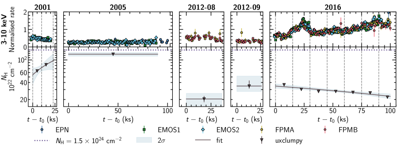
To study the short-term spectral variability of this source, we decide to slice the observation of 2001 in two slices of 10 ks denoted by circled numbers ① and ②. The simultaneous observations of 2016 are sliced in seven slices of 15 ks indexed from ① to ⑦. The start of the EPIC-pn exposure serves as the origin of time for the intervals. The intervals are delimited by dashed vertical lines in the light-curves of Figure 1.

3 Spectral analysis

In this work, the spectral analysis is performed with the X-ray Spectral Fitting Package (XSPEC; Arnaud, 1996) and its Python wrapper PyXspec. We adopt the cross-sections of Verner et al. (1996) and the chemical abundances reported in Wilms et al. (2000).

Cash statistic (C-stat; Cash, 1979) is used to account for the Poisson distribution of photons. The fitting is performed using the Bayesian X-ray Analysis package (BXA; Buchner et al., 2014) bridging XSPEC with nested sampling Monte Carlo algorithm implemented in UltraNest (Buchner, 2016, 2019, 2021). We use nested sampling for its unsupervised global parameter exploration and its naturally self-convergence criterion. We use wide log-uniform priors for normalisation and column density parameters and wide uniform priors for the other parameters. Using samples of the posterior distribution of the parameters, the median of the parameters is estimated. Uncertainties at $68\%$ confidence levels are computed using the 16th and 84th quantiles of the posterior distributions.

Cross-calibration factors between instruments are included in all models. These factors are estimated by fitting the phenomenological model. We assess the goodness of fit through simulations with fakeit in XSPEC using the best-fit value obtained from the fit. We simulate 1000 spectra for each instrument and rebin the spectra with a constant number of channels, 50 and 30, for XMM-Newton and NuSTAR, respectively. The realisations are then plotted against the observed data. Due to the lack of variability below 3 keV, we decided to perform the spectral analysis only above 3 keV. We found a cross-calibration mismatch between XMM-Newton and NuSTAR below $\sim 4$ keV, for that reason we fit NuSTAR data only above that energy.

3.1 Phenomenological model

First, we fitted a phenomenological model to the spectra, which can be written in XSPEC parlance as follows,

$$\centering\texttt{Model =}\texttt{constant}\times\texttt{TBabs}\times(\texttt{cutoffpl}\times\texttt{TBpcf}+\texttt{xillver}).\@add@centering$$ (1)

The first component constant is the cross-calibration factor between the different instruments. The second component TBabs (Wilms et al., 2000) models the absorption of X-ray photons in the line of sight by the gas and dust of our Galaxy with an equivalent hydrogen column density $N_{\mathrm{H}}=1.26\times 10^{20}$  cm^-2(HI4PI Collaboration et al., 2016). The primary X-ray emission from the hot corona is modelled using a power-law with an exponential cutoff (cutoffpl). We tried to let the high-energy cutoff free to vary but no constraints were obtained so it was frozen to 500 keV for all the fits. We accounted for the absorption of the primary emission with TBpcf (Wilms et al., 2000) where the partial covering fraction $f_{\rm cov}$ was left free to vary. As their values converged to unity we fixed $f_{\rm cov}=1$, modelling a fully covering absorber, for the remainder of the analysis. The primary emission in Type-2 sources is thought to be reprocessed by distant neutral material leading to a reflection spectrum that we modelled using xillver (García & Kallman, 2010; García et al., 2013, 2014). xillver is a tabulated model, computed by solving the radiative transfer equation in a plane-parallel geometry for a slab of gas illuminated by an X-ray source. We assume the reflector as distant and neutral, so the ionization parameter $\log\xi$ is frozen to 0. As NGC 7582 is a Seyfert-2 we freeze the inclination of the line of sight with respect to the normal of the disk to $\theta=80^{\circ}$. The photon index and the high-energy cutoff of xillver are tied to the ones of the illuminating power law.

We added a scattered primary emission component in the form of a constant times a power law to account for the scattered emission observed for instance in Turner et al. (1997). The constant was allowed to vary between 0 and 1 to model the scattered fraction, the parameters of the power law are tied to the ones of the primary power law. When fitting the phenomenological model with this component for the first slice of the observations of 2001 and 2016 and the observation of 2005 we find values of the scattered fraction less than $2\%$. These results are consistent with the relation between the column density and the scattered fraction observed in Gupta et al. (2021). In fact, this component is supposed to be more important at soft X-rays, below $\sim 2-3\,\rm keV$, which are not analysed in this work. Thus, we do not include this component in the model as it does not improve the quality of the fit substantially.

3.2 Physically-motivated model

We also use the physical Unified X-ray Clumpy model (uxclumpy; Buchner et al., 2019). This model takes into account Compton scattering, photo-electric absorption and line fluorescence effects due to the absorber. Buchner et al. (2019) produced this clumpy model assuming that the total number of clouds is constant but the observed distribution depends on the geometry of the absorber and the line of sight. The distribution of the angular size of the clumps is computed to reproduce eclipse events in AGN.

Two geometrical parameters are used: TORsigma, i.e. the vertical extent of the cloud population, the smaller this value the more concentrated the clouds in the disc plane; and CTKcover, i.e. the covering factor of the inner ring of clouds, the higher this value the larger the inner clouds. The inclination angle of the line of sight with respect to the normal to the disc is frozen to $80^{\circ}$ as in the phenomenological model.

In XSPEC, the model can be written as follows,

$$\texttt{Model =}\texttt{constant}\times\texttt{TBabs}\times(\texttt{atable[uxclumpy-cutoff]}\\ +\texttt{constant}\times\texttt{atable[uxclumpy-cutoff-omni]}).$$ (2)

As mentioned previously, the first constant component is the cross-calibration factor estimated with the phenomenological model and TBabs models the absorption of X-rays by gas and dust of our Galaxy. The table uxclumpy-cutoff models the spectrum with the reflected and transmitted components as well as fluorescent lines. The table uxclumpy-cutoff-omni models the incident spectrum of the X-ray corona with the power law. This component models unabsorbed emission of the corona, hence it is supposed to model a warm re-emission. The parameters of the uxclumpy-cutoff-omni component are tied to the ones of uxclumpy-cutoff, as they must represent the same geometry. A factor ranging between $10^{-5}$ and $0.1$ is added for the warm emission model uxclumpy-cutoff-omni, this limits the contribution of the warm emission component up to $10\%$ of the transmitted and reflected component.

4 Results

4.1 Phenomenological model

Figure 3: Phenomenological model fitted on all epochs with the spectra (upper panels) and residuals (lower panels). The instruments are plotted as follows: EPIC-pn in dark blue, EPIC-MOS1 in green, EPIC-MOS2 in light blue, FPMA in yellow and FPMB in magenta. The additive individual components of the model are depicted in coloured dashed lines. The circled numbers ①, ②, …, ⑦ indicate the slices corresponding to the given observation.

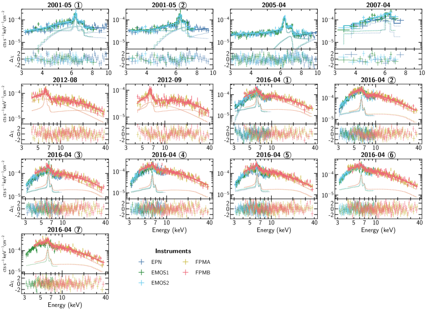
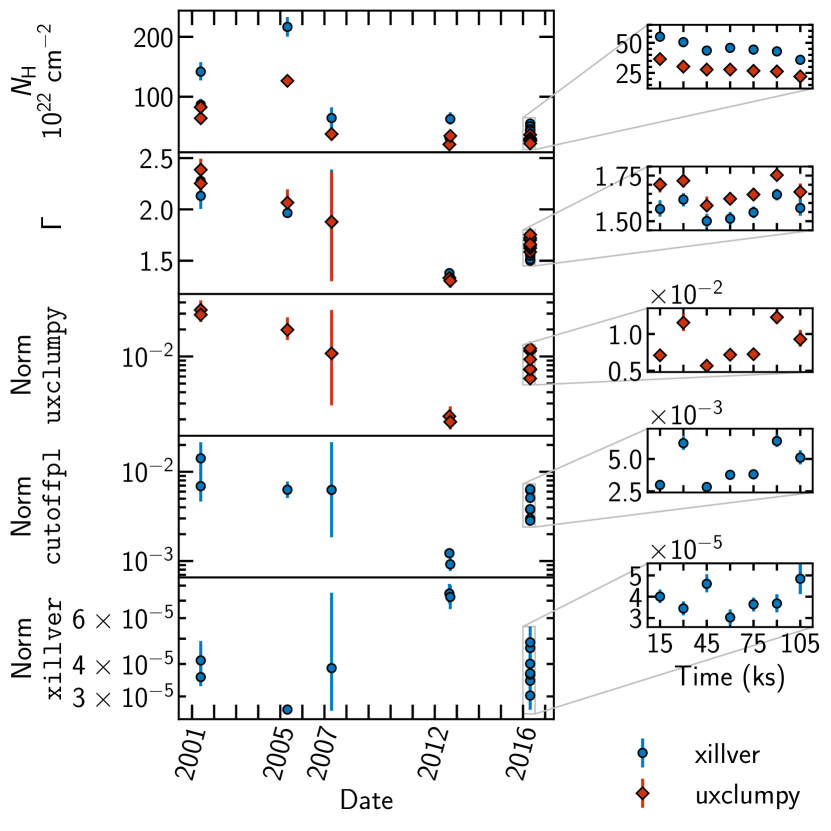
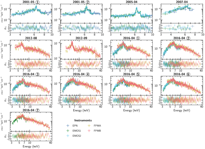
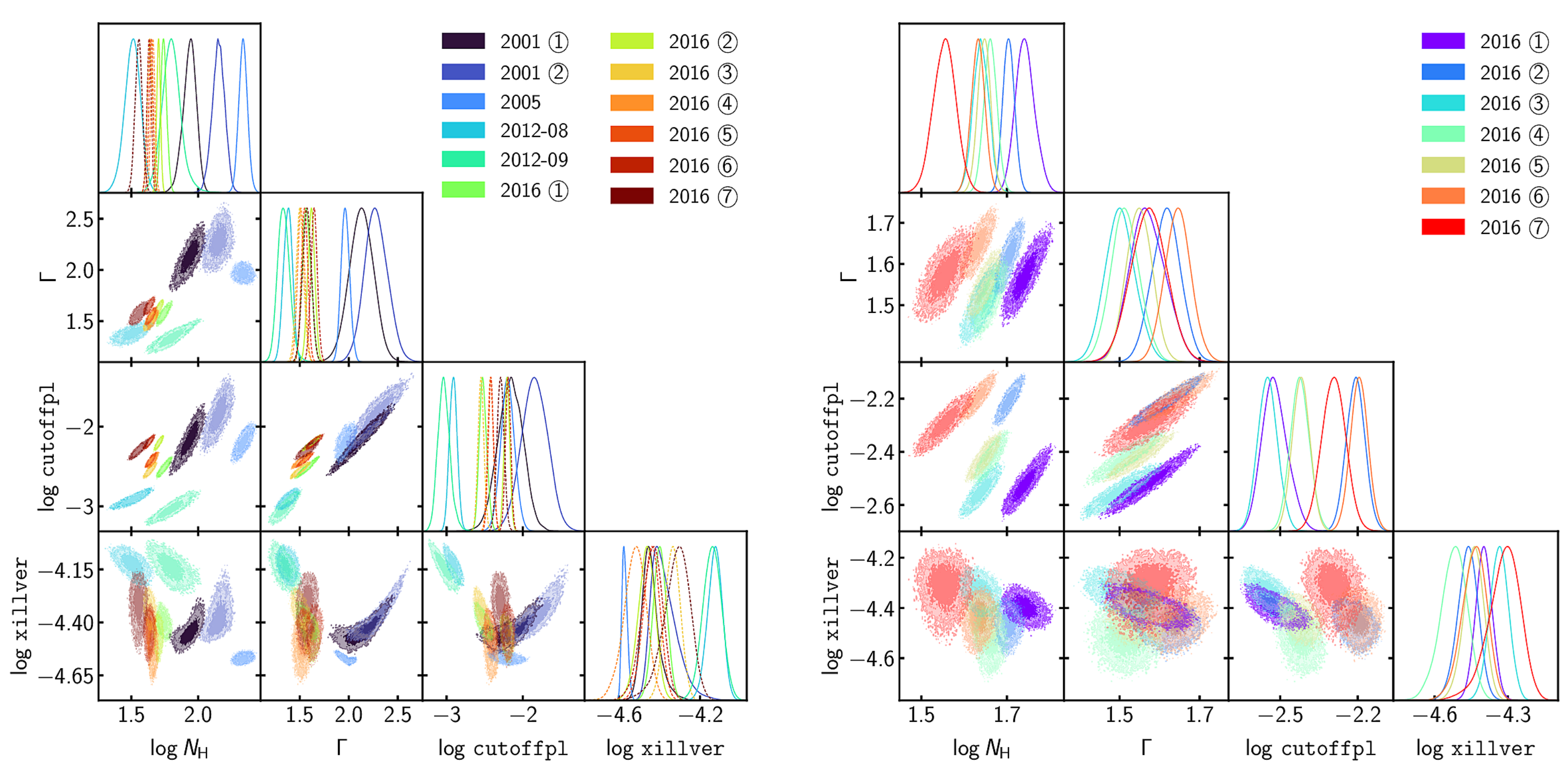
We fit the phenomenological model presented in Section 3.1, finding good fits in all epochs. The best-fit parameters are presented in Table 4, and the fitted spectra are shown in Figure 3 and the samples of the posterior distributions on the parameters are plotted in Figure 11. The evolution of the fitted physical parameters is plotted in blue circles in Figure 4. The values of the cross-calibration factors are presented in Table 8. The cross-calibration factors obtained can be up to $35\%$ between EPIC and FPM instruments and up to $13\%$ between EPIC cameras. As stated in the calibration technical note these factors are expected to be high when using the most recent calibration files.

The photon index value is usually higher when using XMM-Newton data because the data only extend between $3$ and $10$ keV. The column density of the absorber varies between the two slices of the 2001 observation. It increased from $0.87\pm 0.1$ to $1.4\pm 0.2\times 10^{24}$  cm^-2. A hint of softening in $\Gamma$ can also be seen during this observation. However, the two values are consistent within 1-$\sigma$, increasing from $2.1\pm 0.1$ to $2.3\pm 0.1$. The observation of 2005 revealed the highest column density $N_{\mathrm{H}}={2.16}\pm 0.16\times 10^{24}$  cm^-2 and the lowest flux of the reflection component. The two observations of 2012 present the hardest photon index ($\Gamma=1.38\pm{0.05}$ and $\Gamma=1.33\pm 0.06$), and the lowest column density ${0.32}\pm{0.04}\times 10^{24}$  cm^-2. In 2016, the column density decreased continuously from $0.55\pm{0.03}$ to $0.36\pm 0.02\times 10^{24}$  cm^-2 from the start to the end of the observation. In the meantime, the photon index varied as well as the normalisation. Given the low quality of the observation of 2007, only poor constraints on the parameters could be found.

Figure 4: Best fit values of the best physical model (see Section 4.2) (red diamonds) and phenomenological model (blue circles) in all epochs, given within $68\%$-confidence levels. Panels from top to bottom: equivalent hydrogen column density, photon index, normalisation of uxclumpy, normalisation of cutoffpl and normalisation of xillver.

Table 4: Best fit values of the phenomenological model across all epochs. The uncertainties are given with a $68\%$ confidence.
^a Equivalent hydrogen column density modelled with TBpcf in $10^{22}$  cm^-2.
^b Photon index of the power law.
^c Normalisation in $10^{-3}$ ($10^{-5}$) photon keV^-1 s^-1  cm^-2 for cutoffpl (xillver).
^d Flux of the component in unit of $10^{-12}$ erg s^-1  cm^-2 either in the 3-10 keV band or in the 10-40 keV band.
^e Total C-statistic / number of degrees of freedom.

Epoch	${N_{\mathrm{H}}}^{~{}\rm a}$	$\Gamma^{\rm b}$		cutoffpl			xillver		cstat/dof${}^{~{}\rm e}$
			Norm${}^{~{}\rm c}$	F${{}_{\mathrm{3-10}}}^{\rm d}$	F${{}_{\mathrm{10-40}}}^{~{}\rm d}$	Normc	F${{}_{\mathrm{3-10}}}^{\rm d}$	F${{}_{\mathrm{10-40}}}^{\rm d}$
2001-05 {1}⃝	${86.66}^{+{9.6}}_{-{10.0}}$	${2.13}\pm 0.1$	${6.90}^{+{2.9}}_{-{2.3}}$	$10.53_{-2.0}^{+1.8}$	$9.94_{-0.9}^{+0.8}$	${3.56}^{+{0.4}}_{-{0.3}}$	$1.95\pm 0.1$	${7.28}_{-1.6}^{+1.3}$	$113.84/121$
2001-05 {2}⃝	${141.81}^{+{15.7}}_{-{14.4}}$	${2.28}\pm 0.1$	${14.16}^{+{7.2}}_{-{4.7}}$	$16.90_{-4.5}^{+3.5}$	$13.19_{-2.4}^{+2.0}$	${4.13}^{+{0.8}}_{-{0.5}}$	$1.91\pm{0.1}$	${5.96}_{-1.2}^{+1.3}$	$96.40/96$
2005-04	${216.57}^{+{16.4}}_{-{16.1}}$	${1.97}\pm{0.04}$	${6.29}^{+{1.5}}_{-{1.2}}$	$12.73_{-2.5}^{+2.1}$	$14.80_{-2.8}^{+2.3}$	${2.67}^{+{0.09}}_{-{0.08}}$	$1.61\pm{0.04}$	${7.39}\pm 0.6$	$251.29/218$
2007-04	${64.52}^{+{17.8}}_{-{18.2}}$	${1.88}^{+{0.5}}_{-{0.6}}$	${6.27}^{+{15.2}}_{-{4.4}}$	$14.94_{-6.4}^{+3.5}$	$19.32_{-12}^{+5.6}$	${3.85}^{+{3.7}}_{-{1.2}}$	$1.52\pm 0.4$	${8.27}_{-7.2}^{+4.5}$	$29.98/29$
2012-08	${32.36}^{+{4.6}}_{-{4.4}}$	${1.38}^{+{0.04}}_{-{0.05}}$	${1.22}^{+{0.2}}_{-{0.1}}$	$6.91\pm 0.6$	$17.37\pm 1.72$	${7.45}^{+{0.7}}_{-{0.6}}$	$1.93\pm 0.2$	${20.20}\pm 1.8$	$272.41/227$
2012-09	${62.82}^{+{11.2}}_{-{9.1}}$	${1.33}\pm{0.06}$	${0.92}^{+{0.2}}_{-{0.1}}$	$5.61_{-0.7}^{+0.6}$	$14.89_{-1.7}^{+1.6}$	${7.23}^{+{0.8}}_{-{0.7}}$	$1.68\pm 0.2$	${18.72}_{-1.7}^{+1.8}$	$236.79/187$
2016-04 {1}⃝	${55.11}^{+{3.0}}_{-{2.6}}$	${1.57}^{+{0.05}}_{-{0.04}}$	${2.99}^{+{0.4}}_{-{0.3}}$	$12.05_{-0.6}^{+0.5}$	$23.50_{-1.1}^{+1.0}$	${4.01}\pm 0.3$	$1.61\pm{0.12}$	${12.71}\pm 0.9$	$385.72/332$
2016-04 {2}⃝	${50.61}^{+{1.6}}_{-{1.5}}$	${1.62}^{+{0.03}}_{-{0.04}}$	${6.22}\pm{0.5}$	$22.85\pm 0.7$	${41.81}_{-1.7}^{+1.6}$	${3.45}\pm 0.3$	$1.51\pm{0.2}$	${11.20}_{-1.0}^{+1.1}$	$419.22/395$
2016-04 {3}⃝	${43.57}^{+{2.0}}_{-{1.8}}$	${1.50}\pm{0.04}$	${2.83}^{+{0.3}}_{-{0.2}}$	$12.78\pm 0.5$	${27.24}\pm 1.4$	${4.61}^{+{0.5}}_{-{0.4}}$	$1.61\pm 0.1$	${13.94}\pm 1.2$	$382.47/356$
2016-04 {4}⃝	${45.84}\pm 1.6$	${1.51}^{+{0.04}}_{-{0.03}}$	${3.77}\pm{0.3}$	$16.67\pm 0.6$	${34.87}_{-1.7}^{+1.6}$	${3.02}\pm 0.4$	$1.09\pm{0.15}$	${9.23}\pm 1.1$	$436.85/374$
2016-04 {5}⃝	${44.40}^{+{1.5}}_{-{1.6}}$	${1.55}\pm{0.03}$	${3.81}\pm 0.3$	$15.83_{-0.6}^{+0.5}$	${31.75}_{-1.3}^{+1.2}$	${3.64}\pm 0.3$	$1.41\pm{0.2}$	${11.42}\pm 1.0$	$470.41/417$
2016-04 ⑥	${42.89}\pm{1.5}$	${1.65}\pm{0.03}$	${6.38}\pm 0.5$	$22.41\pm 0.9$	${39.60}_{-2.0}^{+1.9}$	${3.68}\pm 0.4$	$1.68\pm 0.2$	${11.98}\pm 1.4$	$435.84/386$
2016-04 {7}⃝	${35.88}\pm 2.2$	${1.57}^{+{0.05}}_{-{0.04}}$	${5.10}^{+{0.6}}_{-{0.5}}$	$20.30_{-1.3}^{+1.2}$	${39.48}\pm 3.0$	${4.84}\pm 0.7$	$1.95\pm{0.30}$	${15.40}\pm 2.4$	$232.30/227$

4.2 Physical model

Assuming the geometry of the absorber does not change over time, we expect to find a unique geometry fitting to the data for all epochs. We fitted the physical model on all epochs by freezing the geometrical parameters TORsigma and CTKcover. We performed the fits for eleven out of twenty available geometries because we do not use the geometries which do not include clumps (where ${\tt TORsigma}=0$) or which include large clouds in the thick ring of clouds, i.e. where ${\tt CTKcover}=0.6$.

UltraNest provides an estimate of the marginal likelihood also called evidence $Z$ and samples of the posterior probability distributions. Assuming two models $M_{1}$ and $M_{2}$ with respective evidences $Z_{1}$ and $Z_{2}$, the Bayes factor $K$ is the ratio of the two marginal likelihoods, i.e. $K={Z_{1}}/{Z_{2}}$. Jeffreys (1939) gives an empirical interpretation of the values of the Bayes factor, which can be used for model selection. For instance, if $K<1$, then model $M_{1}$ is rejected, if $10<K<10^{3/2}$, model $M_{1}$ is supported with strong evidence over model $M_{2}$.

Table 9 shows the natural logarithm of the evidence for the eleven geometries fitted. We sum the logarithm of the evidence over all epochs and use it as a criterion to select the three geometries with the highest $\ln Z$. This rules out the geometries dominated by the inner ring of clouds (with ${\tt TORSigma}=7$) and the partial covering geometry associating clumps and larger thick clouds (${\tt TORSigma}=28$). All the accepted geometries consist of a fully covering clumpy absorber (${\tt TORsigma}=84$).

Figure 5: Best-fit geometry of the fully covering clumpy geometry of the physical model fitted on all epochs with the spectra (upper panels) and residuals (lower panels). The instruments are plotted as follows: EPIC-pn in dark blue, EPIC-MOS1 in green, EPIC-MOS2 in light blue, FPMA in yellow and FPMB in magenta. The circled numbers ①, ②, …, ⑦ indicate the slices corresponding to a given observation.

Table 5: Best fit values of the fully covering clumpy geometry of the physical model. The uncertainties are given with a $68\%$ confidence.
^a Equivalent hydrogen column density modelled with uxclumpy in $10^{22}$  cm^-2.
^b Photon index of the power law.
^c Normalisation in $10^{-3}$ photon keV^-1 s^-1  cm^-2.
^d Total C-statistic / number of degrees of freedom.

Epoch	${N_{\mathrm{H}}}^{~{}\rm a}$	$\Gamma^{~{}\rm b}$	uxclumpy	factor	cstat/dof${}^{~{}\rm d}$
			Norm${}^{~{}\rm c}$	$\times 10^{-2}$
2001-05 ①	${64.10}\pm{3.7}$	${2.39}\pm 0.1$	${32.97}^{+{9.0}}_{-{5.9}}$	${8.79}^{+{0.9}}_{-{1.4}}$	$123.05/123$
2001-05 ②	${82.60}^{+{6.0}}_{-{5.3}}$	${2.25}\pm 0.1$	${29.16}^{+{8.0}}_{-{4.9}}$	${8.99}^{+{0.8}}_{-{1.3}}$	$94.92/98$
2005-04	${126.51}^{+{4.5}}_{-{4.6}}$	${2.07}\pm 0.1$	${19.79}^{+{7.5}}_{-{4.5}}$	${6.86}^{+{1.4}}_{-{1.3}}$	$252.08/220$
2007-04	${37.76}^{+{10.9}}_{-{10.3}}$	${1.88}^{+{0.5}}_{-{0.6}}$	${10.82}^{+{22.1}}_{-{8.0}}$	${6.44}^{+{2.4}}_{-{2.9}}$	$30.11/31$
2012-08	${20.43}^{+{2.6}}_{-{2.5}}$	${1.33}^{+{0.04}}_{-{0.05}}$	${2.16}^{+{0.4}}_{-{0.3}}$	${6.93}^{+{2.3}}_{-{3.6}}$	$291.17/228$
2012-09	${34.63}^{+{8.7}}_{-{3.4}}$	${1.30}^{+{0.1}}_{-{0.07}}$	${1.87}^{+{0.9}}_{-{0.3}}$	${7.99}^{+{1.6}}_{-{3.5}}$	$250.03/188$
2016-04 ①	${36.54}^{+{1.4}}_{-{1.5}}$	${1.70}\pm{0.04}$	${7.11}\pm 0.8$	${9.45}^{+{0.4}}_{-{0.8}}$	$379.67/336$
2016-04 ②	${30.26}^{+{1.6}}_{-{1.4}}$	${1.72}^{+{0.03}}_{-{0.04}}$	${11.55}^{+{1.2}}_{-{1.1}}$	${2.73}\pm 1.3$	$429.12/399$
2016-04 ③	${27.80}^{+{1.9}}_{-{1.5}}$	${1.59}^{+{0.05}}_{-{0.03}}$	${5.69}^{+{0.8}}_{-{0.6}}$	${8.33}^{+{1.2}}_{-{2.4}}$	$384.70/360$
2016-04 ④	${27.79}^{+{0.9}}_{-{0.8}}$	${1.62}^{+{0.03}}_{-{0.03}}$	${7.17}^{+{0.6}}_{-{0.5}}$	${2.04}^{+{1.9}}_{-{1.4}}$	$440.63/378$
2016-04 ⑤	${26.74}^{+{0.9}}_{-{0.8}}$	${1.65}\pm{0.03}$	${7.26}^{+{0.6}}_{-{0.5}}$	${2.05}^{+{2.2}}_{-{1.5}}$	$463.93/421$
2016-04 ⑥	${26.22}^{+{1.0}}_{-{0.9}}$	${1.75}^{+{0.02}}_{-{0.03}}$	${12.28}\pm{0.9}$	${1.97}^{+{2.5}}_{-{1.4}}$	$433.36/389$
2016-04 ⑦	${22.07}^{+{1.5}}_{-{1.4}}$	${1.66}\pm{0.05}$	${9.29}^{+{1.3}}_{-{1.0}}$	${4.13}^{+{3.6}}_{-{2.9}}$	$231.85/229$

We compute the Bayes factor for the selected geometries in Table 6 with respect to the best geometry. The Bayes factor is then defined as: $\ln K=\ln Z_{(84,0)}-\ln Z$. Using the Jeffrey scale (Jeffreys, 1939), we notice that $K>10^{2}$, hence the fully covering clumpy geometry (${\tt TORSigma}=84$ and ${\tt CTKCover}=0$) is statistically favoured over all geometries and the phenomenological model.

Table 6: Values of the natural logarithm of the evidence $Z$ and of the Bayes factor $K$ for the best three geometries and the phenomenological model.
The geometries are visualisations of the absorber as seen by the X-ray source. Extracted from the uxclumpy webpage, courtesy of Johannes Buchner.

Model	Evidence $\ln Z$	Bayes factor $\ln K$
(84,0)      $\begin{array}[]{l}\includegraphics[width=21.33955pt]{figures/appendix/geometries/84-0.png}\end{array}$	$-2106$	-
(84,0.2) $\begin{array}[]{l}\includegraphics[width=21.33955pt]{figures/appendix/geometries/84-0.2.png}\end{array}$	$-2111$	$5$
(84,0.3) $\begin{array}[]{l}\includegraphics[width=21.33955pt]{figures/appendix/geometries/84-0.3.png}\end{array}$	$-2129$	$23$
xillver	$-2187$	$81$

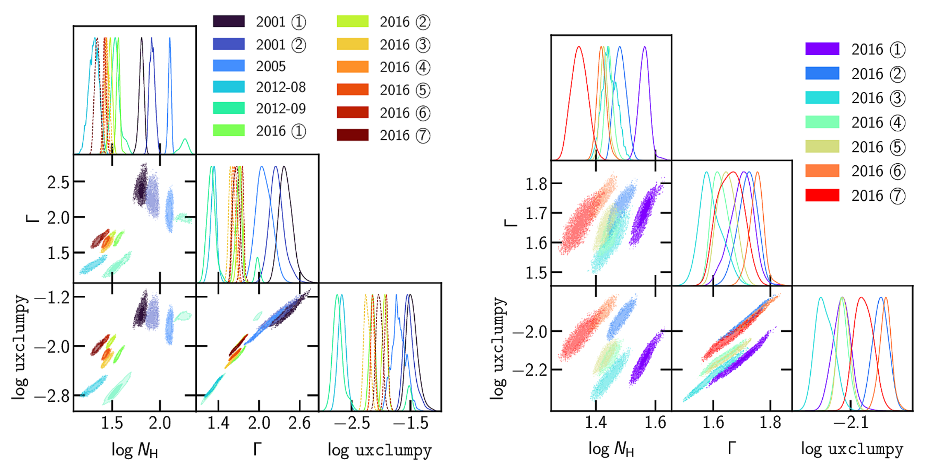
Figure 4 shows the best-fit parameters obtained using this geometry in red diamonds and in blue circles the best-fit parameters of the phenomenological model. In Figure 5, we show this model fitted to all epochs and give the values of the parameters in all epochs in Table 5. The samples of the posterior distributions on the parameters for this geometry are plotted in Figure 12.

The values of $\Gamma$ in all epochs are found to be larger than the ones obtained using the phenomenological model, however they are all consistent within 2 $\sigma$. Values of $N_{\mathrm{H}}$ of the physical model are smaller than values of the phenomenological model but they follow the same variations. This is most likely due to the different assumptions of each of the models. The normalisation of uxclumpy follows also the same trend as the one of the cutoffpl.

5 Discussion

5.1 The origin of the variability

In Figure 6, we plot the fluxes in the 3-40 keV energy band for the primary X-ray emission and the reflection component of the phenomenological model. The 10-40 keV fluxes in the XMM-Newton observations are obtained by extrapolating the best-fit model to larger energy bands. The fluxes are obtained with flux command of XSPEC, on each individual component, i.e cutoffpl and xillver, for all samples of the posterior distribution. The median and the 16${\rm th}$ and 84${\rm th}$ quantiles of the flux distributions are then computed to estimate the $68\%$ confidence levels. We use the phenomenological model as a proxy for distinguishing the contribution of the reflection from one of the power-law. The separation between these two components cannot be done using our current modelling with uxclumpy. The flux of both components varies over long timescales. However, at short timescale, the reflection component appears to be less variable than the power law (this can be seen in the observation of 2016). This suggests that the response of the reflecting component to the incident primary X-ray emission is not instantaneous. As the observation is $100$ ks long, the reflecting/absorbing material must be located at a distance of $d>t_{\mathrm{obs}}\times c\sim 400$ $R_{\mathrm{g}}$ away from the X-ray source. This would put the absorber farther from the black hole, in the BLR.

Figure 6: Unabsorbed flux of the power law and reflection components of the phenomenological model in the 3-40 keV band. The fluxes are in units of $10^{-12}$  erg cm^-2 s^-1. The solid lines in each of the panels represent the weighted mean in the given panel and the shaded areas represent the $1\,\sigma$, $2\,\sigma$ and $3\,\sigma$ levels (shades of green in the full panel and red to yellow in the zoomed panel).

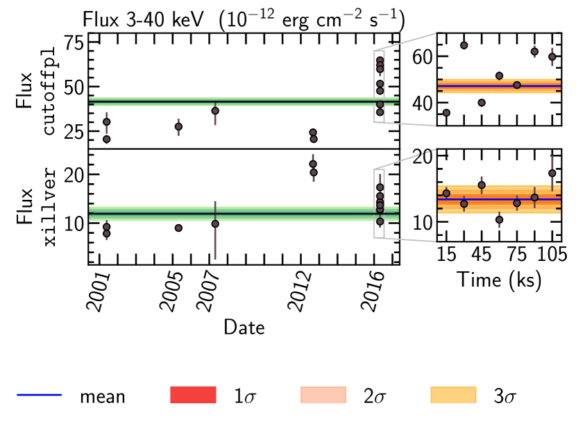
Figures 6 and 7 demonstrate that the variability on both short- and long-timescales is due to an interplay between intrinsic and absorption-induced variations. NGC 7582 exhibited at least three episodes of nearly Compton-thick state (with $N_{\rm H}>10^{24}~{}\rm cm^{-2}$) between 2005 and 2014, which could explain the Changing-look classification of this source. It is worth noting that in 2007, $N_{\rm H}$ may have increased continuously from $4.4_{-0.2}^{+0.3}\times 10^{23}~{}\rm cm^{-2}$ to $(12\pm 2)\times 10^{23}~{}\rm cm^{-2}$ over the course of six months. However, due to the lack of intense monitoring and long observations during this period it is hard to tell whether indeed this rise was continuous or if it also varied on short timescales, similar to the behaviour of the source in 2016. The same reasoning can be applied in 2012, where we observe a decrease of $N_{\mathrm{H}}$ between observations separated by fifteen days but with no way to probe the short-term variability.

In 2001 and 2016, the source exhibited a strong absorption variability. To study this short-term absorption variability, we fitted the evolution of $N_{\mathrm{H}}$ with a linear function in these observations using UltraNest. It is worth noting that this model is employed to evaluate the rate at which $N_{\mathrm{H}}$ varies without having any physical motivation. The results are presented in Table 7. As shown in Figure 8, we observe a sharp increase in $N_{\mathrm{H}}$ in 2001 compared to a slower decrease in 2016. On the contrary, the absorption was constant over 100 ks during the 2005 observation and over $\sim 25$ ks during the observations of 2012. The absence of short-term variability during the 2005 observations suggests that the X-ray emission is absorbed by the same dense absorber during the whole observation.

Figure 7: Historical values of the photon index $\Gamma$, the column density $N_{\mathrm{H}}$ and the observed flux in the 2-10 keV band for NGC 7582. The values from the literature (available in Table 10) are in coloured circles whereas the values obtained with the phenomenological model in this work are in coloured diamonds.

The behaviour of the absorber in the different observations can be summarised as follows: a sharp increase in $N_{\mathrm{H}}$ (while being Compton thin) in 2001, a constant high $N_{\mathrm{H}}$ ($>10^{24}~{}\rm cm^{-2}$) absorption over 100 ks in 2005, an increase of $N_{\mathrm{H}}$ between fifteen days in 2012 and a slow decrease in $N_{\mathrm{H}}$ over 100 ks in 2016. These independent episodes could correspond to occultations by various clumps, in agreement with the favoured physical model of a clumpy medium. If the different clumps have similar structures, then these events could agree with a scenario in which the absorbing BLR clouds have a ‘cometary’ structure, with a dense head and a gradually less dense tail. This structure has been proposed to explain the observed eclipsing events in NGC 1365 (Maiolino et al., 2010) and Mrk 766 (Risaliti et al., 2011). If this were true, then the observation of 2001 would correspond to the start of an eclipsing event, the observation of 2005 would correspond to the obscuration by the dense head of the comet, and the observation of 2016 would correspond to the end of an eclipse where the tail of the comet is obscuring the line of sight. However, this scenario cannot be confirmed or ruled out as none of the observations could represent a full eclipse.

An alternative explanation for the short-term variability is a spherical clump with a density profile peaking in the core and slowly decreasing towards the surface of the clump. The scenario of an eclipse is still valid for a spherical cloud. Thus, longer observations and a closer monitoring may be required to better understand the structure of the absorber in this source.

Observation	slope ($10^{22}$  cm-2$\,\mathrm{ks}^{-1}$)	offset ($10^{22}$  cm-2)
2001-05-25	$1.80_{-0.96}^{+0.96}$	$54.99_{-8.91}^{+9.00}$
2016-04-28	$-0.12_{-0.02}^{+0.02}$	$34.58_{-1.51}^{+1.50}$

Table 7: Best fit values of the parameters of the linear function fitted onto the evolution of the column density. Errors are given with a $68\%$ confidence level.

Figure 8: Evolution of the column density of the clumpy absorber (triangles) as a function of time in the observations of 2001, 2005, 2012 and 2016 (bottom panel). The solid line is a linear fit and the shaded area represents the $2\sigma$ level. The Compton-thick column density is delimited by a purple dotted line. The light-curves of XMM-Newton EPIC instruments and the NuSTAR FPM instruments in the 3-10 keV band are plotted in the upper-panel, see Figure 1 for more details.

5.2 Determining the properties of the BLR clouds

Assuming that the obscuring clouds are located in the BLR, following a Keplerian orbit, we derive below some of the properties of these clouds.

Velocity: Aretxaga et al. (1999) observed NGC 7582 in a Seyfert-1 state with broad optical lines on the 11 July 1998. The estimated FWHM of the H$\alpha$ and H$\beta$ lines is FWHM$=12400$  km s^-1; over the timescale of a few months the FWHM decreased to reach $6660$  km s^-1  at the end of October 1998 (Aretxaga et al., 1999). Ricci et al. (2018) reported a FWHM of $2382\pm 44$  km s^-1, in an observation of 2004. With a 2014 Chandra observation, Braito et al. (2017) estimated the FWHM of the Fe K$\alpha$ line to be FWHM$=1500_{-800}^{+900}$  km s^-1, thus $v=637$  km s^-1. Because no measurement of the FWHM of H$\alpha$ was made close to our observations, it is impossible to predict the state of the source in the optical at the time of our archival observations. We tried to estimate the FWHM of the Fe K$\alpha$ in our XMM-Newton observations but the uncertainties were too high to draw any conclusions. We use the most recent measurement by Braito et al. (2017) to provide a lower limit on the velocity of the clouds: $v\geq 637$  km s^-1.

Size of the clouds: As we do not observe complete eclipsing events, we can only set lower limits on the size of the clouds. The typical duration of an eclipse is at least twice the exposure time $t_{\mathrm{exp}}=100$ ks. Assuming a spherical cloud of diameter $D_{c}$ moving at a velocity $v_{c}$, the duration of an eclipse is $t_{\mathrm{ec}}=D_{c}/v_{c}$. The diameter of the cloud is then $D_{c}\geq 2v_{c}\times t_{\mathrm{exp}}$. Using the value of velocity obtained above, $D_{c}\gtrsim 1.5$ $R_{\mathrm{g}}$ ($1.2\times 10^{13}$ cm).

Location of the BLR: Assuming a Keplerian circular orbit for the clumps in the BLR. The radius of the orbit in the BLR is given by $R=\frac{GM}{v^{2}}=c^{2}/v^{2}$ $R_{\mathrm{g}}$, this gives an upper limit on the location of the clouds in the BLR, $R_{\rm BLR}/R_{g}\lesssim 22000$, $R_{\rm BLR}\sim 0.6$ pc.

5.3 Comparison with previous works

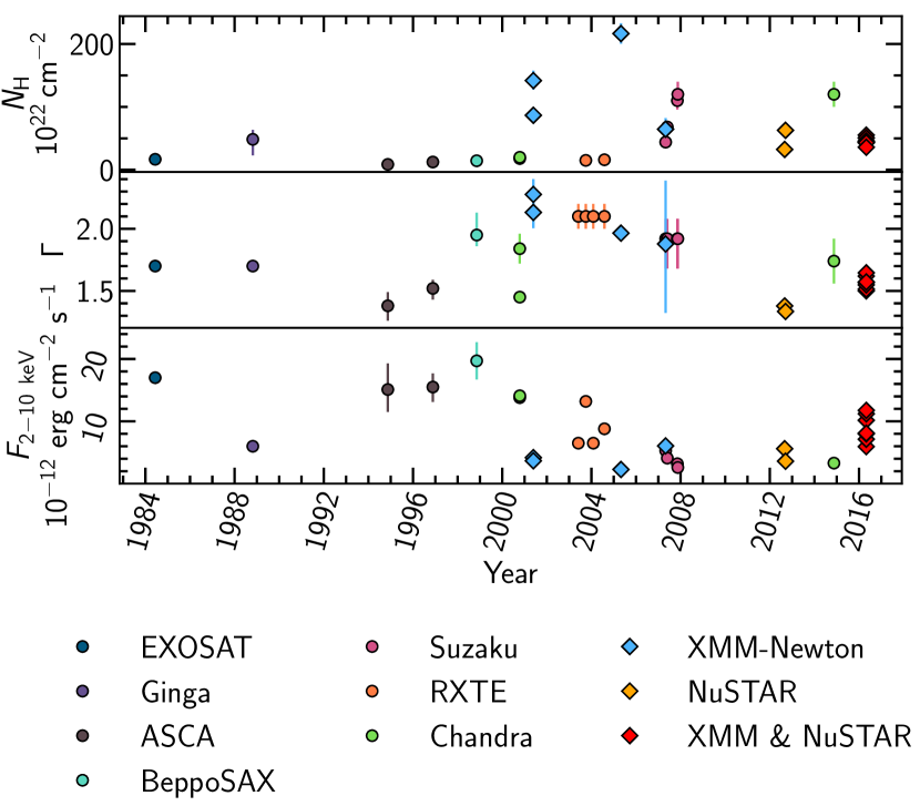
NGC 7582 has been observed by many X-ray observatories. In Figure 7, we plot the values of the column density, the photon index, and the observed flux obtained from previous studies (in circles) and the ones obtained in this work (in diamonds). The previous works mostly used phenomenological models, thus we show the parameters obtained with our best-fit phenomenological model, for consistency. The long-term variability is visible since early observations. As seen in this figure, BeppoSAX observed NGC 7582 in an unobscured state, as opposed to the very absorbed state of 2005 seen by XMM-Newton. We provide a non-exhaustive list of values from the literature in Table 10, where we did not include results from the five observations with the Einstein observatory as it was not possible to get access to all the fitted parameters. Below, we present a comparison between the values reported in the literature to the ones obtained in this work.

Observation 2001: For this observation, the values of the photon index obtained in this work are consistent with the values obtained by Dewangan & Griffiths (2005) and Piconcelli et al. (2007). The value of $N_{\mathrm{H}}$ obtained in the two works are in the same order of magnitude as the value found in slice ①. It is worth noting that Piconcelli et al. (2007) used a two-absorber model. Thus, we compare only with the highest column density, as the fitting range we adopt ($E\geq 3\,\rm keV$) is not sensitive to the low column density absorber.

Observation 2005: In this observation, the column density and photon index obtained by Piconcelli et al. (2007) are also consistent with the ones obtained in this work. Laha et al. (2020) fitted a double-absorber model on this observation and the total column density as well as the photon index are consistent with our work.

Observation 2007: Bianchi et al. (2009) fitted simultaneously the Suzaku observations with the XMM-Newton observation of 2007. Given the poor quality of our data the values are poorly constrained and de facto consistent with values from the literature (e.g., Laha et al., 2020).

Observation 2012: For the NuSTAR observations of 2012, the values of $N_{\mathrm{H}}$ are consistent with the findings of Rivers et al. (2015). However, the values of $\Gamma$ are smaller than the ones found previously ($1.33$ against $1.78$). It worth mentioning that they fitted simultaneously the first observation with a Swift observation and tied several parameters between the two observations of 2012.

Observation 2016: Tanimoto et al. (2022) applied a physical clumpy model (XCLUMPY; Tanimoto et al., 2019) to the time-averaged spectrum of the observation of 2016. Baloković et al. (2018) applied a torus model to the NuSTAR observation only. The values of $\Gamma$ and $N_{\mathrm{H}}$ we obtain on average are consistent with the ones obtained by both Tanimoto et al. (2022) and Baloković et al. (2018). These works found a covering factor of $80-90\%$ which is roughly consistent with our full covering geometry. It is worth noting that these papers did not study the short-term variability seen in this observation.

5.4 Prospects with future X-ray missions

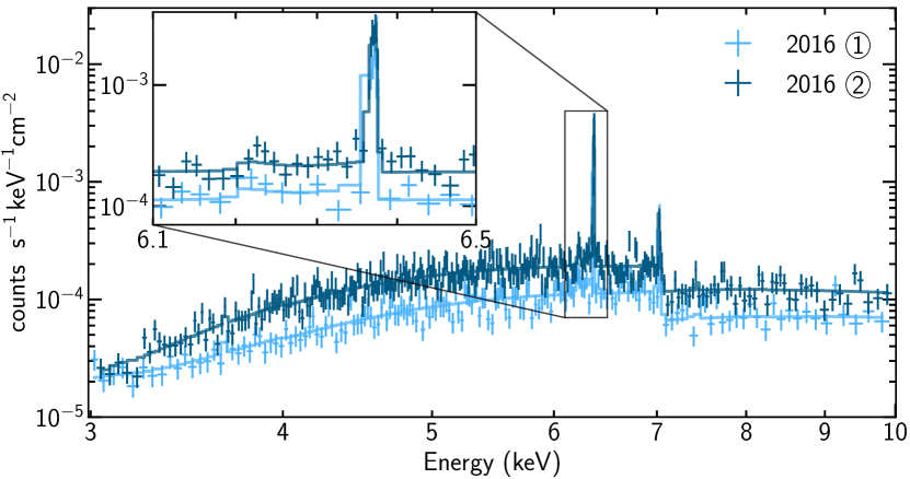
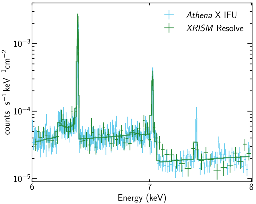
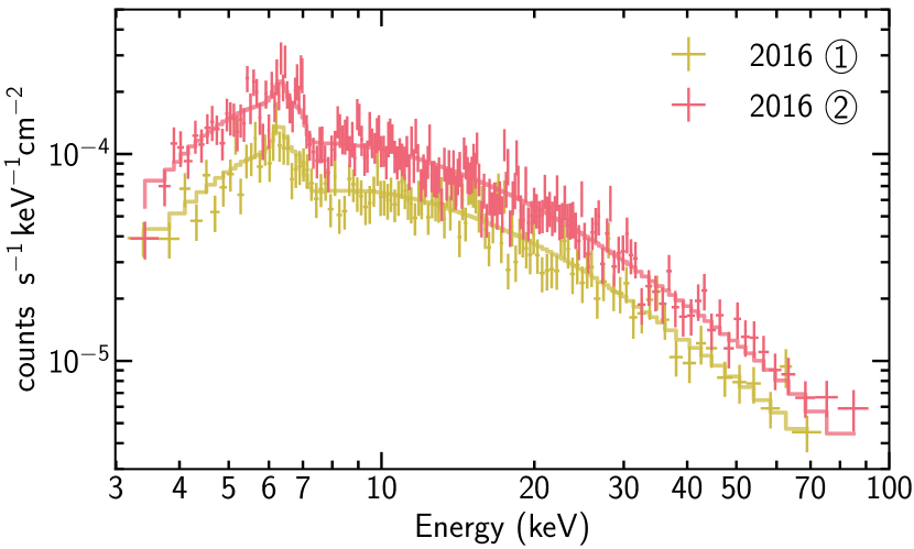
Future X-ray missions will bring the opportunity to improve the current work and better constrain the physical parameters. We simulate data for several instruments assuming the best-fit fully covering model with uxclumpy and we rebin all spectra with at least 25 counts per bin. In Figure 9(a), we show two simulated Athena/X-IFU (Barret et al., 2022) spectra for the observation of 2016 with an exposure time of 5 ks each. Thanks to the large effective area and the high resolution of Athena/X-IFU, it will be possible to probe the spectral variability on shorter timescales with better constraints. In Figure 9(b), we show simulated spectra for the observation of 2005 with an exposure time of 90 ks with Athena/X-IFU and XRISM/Resolve (Tashiro et al., 2020). The inset of Figure 9(a) and Figure 9(b) show a view in the 6.1-6.5 keV range. The Fe K$\alpha$ doublet at 6.404 keV and 6.391 keV cannot be resolved, nevertheless the Compton shoulder can be observed with the 90-ks simulations. Athena and XRISM will enable high-resolution spectroscopy of the low-luminosity state of the AGN as observed in the observation of 2005. Finally, with the High-Energy Telescope (HET) of the concept mission HEX-P (Madsen et al., 2018), observations above 10 keV could constrain both the photon index and the high-energy cutoff. In Figure 10, we show two simulated HET spectra for the observation of 2016 with an exposure time of 5 ks each. Thus, each of these three instruments will enable a better understanding of both the accretion in AGN but also the geometry of the absorbing material surrounding the X-ray source.

(a) Athena/X-IFU

(b) Athena/X-IFU and XRISM/Resolve.

Figure 9: Simulations of spectra with microcalimeter detectors assuming the best-fit uxclumpy model. On the left, simulations of the first two slices of 2016, using Athena/X-IFU with an exposure time of 5 ks. The simulated spectrum of the first slice is in light blue and the second slice is in dark blue. On the right, simulations of the observation of 2005, using Athena/X-IFU (in cyan) XRISM/Resolve (in green) with an exposure time of 90 ks. The spectra are shown in the 6-8 keV range. The inset shows a zoom in the 6.1-6.5 kev range where the Fe K$\alpha$ and the Compton shoulder are resolved.

Figure 10: Simulated HEX-P/HET spectra of the first two slices of 2016 with an exposure time of 5 ks assuming the best-fit uxclumpy model.

6 Conclusions

To model the spectra we have used two different models, a physically-motivated model accounting for the geometry of the absorber and a phenomenological model. The main results can be summarised as follows:

• The absorption is best described by a fully covering clumpy absorber. This geometry is statistically favoured using Bayes factors.

• Long-term and short-term variability are due to intrinsic changes in the X-ray luminosity of the source, and changes in the absorption in the line of sight. The latter can explain the changing-look classification of this source, more specifically changing-obscuration, as the source switches between Compton-thick and Compton-thin due to changes in the obscuring column along the line of sight, respectively.

• The absorber is located at a distance not larger than $0.6$ pc.

• Assuming a single cloud in the line of sight, we estimate the size of the cloud to be larger than $10^{13}$ cm, for a velocity of $\sim 700$  km s^-1.

• Given the variety of behaviour of the absorption at different timescales, and the fact that the observations are not long enough to constrain a full eclipsing event, we cannot make strong arguments on the shape of the clouds. However, our results strongly suggest the presence of a variety of cloud densities, or even a gradient in the density within a single cloud (as seen in 2016), favouring comet-shaped clouds or at least a non-uniform cloud.

Data Availability

The data used in this paper are publicly available to access and download from the High Energy Astrophysics Science Archive Research Center for NuSTAR and from the XMM-Newton Science Archive. Final data products from this study can be provided on reasonable request to the corresponding author.

Appendix A Tables and Figures

Table 8: Calibration factors across all epochs for all instruments. The uncertainties are given with a $68\%$ confidence.

Epoch			Instruments
	EPN	EMOS1	EMOS2	FPMA	FPMB
2001-05 ①	1	$1.08_{-0.05}^{+0.04}$	$1.08_{-0.04}^{+0.05}$	-	-
2001-05 {2}⃝	1	$1.08_{-0.05}^{+0.05}$	$1.02_{-0.05}^{+0.05}$	-	-
2005-04	1	$1.04_{-0.02}^{+0.02}$	$1.08_{-0.02}^{+0.02}$	-	-
2007-04	1	$1.19_{-0.09}^{+0.09}$	$1.25_{-0.08}^{+0.06}$	-	-
2012-08	-	-	-	1	$0.98_{-0.02}^{+0.02}$
2012-09	-	-	-	1	$1.00_{-0.03}^{+0.03}$
2016-04 {1}⃝	1	$1.04_{-0.03}^{+0.03}$	$1.10_{-0.03}^{+0.03}$	$1.31_{-0.03}^{+0.03}$	$1.28_{-0.04}^{+0.03}$
2016-04 {2}⃝	1	$1.09_{-0.03}^{+0.03}$	$1.06_{-0.02}^{+0.03}$	$1.26_{-0.03}^{+0.03}$	$1.20_{-0.03}^{+0.03}$
2016-04 {3}⃝	1	$1.02_{-0.03}^{+0.03}$	$1.09_{-0.03}^{+0.04}$	$1.27_{-0.04}^{+0.04}$	$1.27_{-0.04}^{+0.04}$
2016-04 {4}⃝	1	$1.04_{-0.03}^{+0.03}$	$1.11_{-0.03}^{+0.03}$	$1.26_{-0.04}^{+0.04}$	$1.28_{-0.04}^{+0.04}$
2016-04 {5}⃝	1	$1.08_{-0.03}^{+0.03}$	$1.13_{-0.03}^{+0.03}$	$1.29_{-0.03}^{+0.03}$	$1.34_{-0.02}^{+0.01}$
2016-04 {6}⃝	-	1	$1.06_{-0.03}^{+0.03}$	$1.24_{-0.03}^{+0.04}$	$1.25_{-0.04}^{+0.04}$
2016-04 {7}⃝	-	1	-	$1.25_{-0.05}^{+0.05}$	$1.25_{-0.04}^{+0.05}$

Figure 11: Contours of the samples of the posterior distributions of the parameters of the phenomenological model. For all epochs (left) and all slices of the observation of 2016 (right).

Table 9: Values of $\ln Z$ for eleven geometries of the physical model and the phenomenological model over all epochs. The gradient of colour shows for each row maximal values (dark blue) to minimal (yellow). The last row gives the total $\ln Z$ for all epochs. The geometries are visualisations of the absorber as seen by the X-ray source. Extracted from the uxclumpy webpage, courtesy of Johannes Buchner.

Epoch	xillver	Geometries uxclumpy    (TORsigma, CTKcover)
		(7,0)	(7,0.3)	(7,0.5)	(28,0)	(28,0.2)	(28,0.3)	(28,0.5)	(84,0)	(84,0.2)	(84,0.3)	(84,0.5)
2001 {1}⃝	-77	-97	-113	-108	-83	-88	-93	-106	-76	-80	-85	-99
2001 {2}⃝	-68	-74	-80	-79	-62	-65	-68	-78	-62	-64	-67	-73
2005	-149	-177	-196	-204	-159	-171	-176	-201	-142	-145	-149	-161
2007	-30	-27	-27	-27	-26	-26	-26	-27	-26	-26	-27	-27
2012-a	-156	-172	-174	-180	-167	-167	-170	-175	-161	-159	-160	-163
2012-b	-137	-143	-142	-140	-132	-134	-136	-148	-140	-139	-139	-143
2016 {1}⃝	-220	-230	-243	-235	-210	-212	-216	-227	-208	-212	-219	-235
2016 {2}⃝	-238	-233	-238	-234	-226	-224	-225	-228	-231	-230	-228	-225
2016 {3}⃝	-219	-237	-243	-237	-215	-216	-220	-229	-209	-209	-211	-218
2016 {4}⃝	-246	-243	-244	-243	-236	-235	-236	-239	-237	-237	-236	-235
2016 {5}⃝	-265	-271	-274	-270	-254	-253	-255	-262	-248	-247	-247	-249
2016 {6}⃝	-244	-245	-247	-245	-235	-235	-237	-242	-234	-234	-234	-235
2016 {7}⃝	-138	-139	-138	-136	-132	-131	-131	-133	-131	-129	-129	-129
Sum	-2187	-2289	-2360	-2337	-2137	-2157	-2188	-2293	-2106	-2111	-2129	-2192

Figure 12: Contours of the samples of the posterior distributions of the parameters of the physical model’s best geometry. For all epochs (left) and all slices of the observation of 2016 (right).

Table 10: Historical values of the photon index $\Gamma$, the column density $N_{\mathrm{H}}$ and observed flux in the 2-10 keV band.^† refers to parameters frozen or tied during the fits.

Date	Observatory	$\Gamma$	$N_{\mathrm{H}}$ $10^{22}~{}\mathrm{cm}^{-2}$	Flux $(2-10)$ keV $10^{-12}$  erg cm-2 s-1	Reference
1984-06-09	EXOSAT	$1.70$	$16.70_{-4.90}^{+5.80}$	$17$	Turner & Pounds (1989)
1988-10-25	Ginga	$1.70$	$48.40_{-15.20}^{+25.40}$	$6$	Warwick et al. (1993)
1994-11-14	ASCA	$1.38_{-0.11}^{+0.12}$	$8.60_{-0.80}^{+0.80}$	$15.10_{-4.20}^{+3.60}$	Turner et al. (1997)
1996-11-21	ASCA	$1.52_{-0.07}^{+0.09}$	$12.40_{-0.80}^{+0.60}$	$15.50_{-2.20}^{+2.40}$	Xue et al. (1998)
1998-11-09	BeppoSAX	$1.95_{-0.18}^{+0.09}$	$14.40_{-1}^{+0.90}$	$19.70_{-3}^{+3}$	Turner et al. (2000)
2000-10-14	Chandra	$1.84_{-0.12}^{-0.12}$	$17.95_{-2.11}^{+2.11}$	$13.8$	Laha et al. (2020)
2000-10-15	Chandra	$1.45^{\dagger}$	$19.9_{-3.85}^{+3.85}$	$14.1$	Laha et al. (2020)
2001-05-25	XMM-Newton	$1.90_{-0.02}^{+0.05}$	$54.90_{-2.10}^{+6.60}$	$4$	Piconcelli et al. (2007)
2003-06-01	RXTE	$2.10_{-0.10}^{+0.10}$	-	$6.50_{-0.60}^{+0.60}$	Rivers et al. (2015)
2003-10-01	RXTE	$2.10^{{\dagger}}$	$15_{-2}^{+2}$	$13.20_{-0.60}^{+0.20}$	Rivers et al. (2015)
2004-02-01	RXTE	$2.10^{\dagger}$	-	$6.50_{-0.20}^{+0.20}$	Rivers et al. (2015)
2004-08-01	RXTE	$2.10^{\dagger}$	$16_{-5}^{+5}$	$8.80_{-0.20}^{+0.20}$	Rivers et al. (2015)
2005-04-29	XMM-Newton	$1.93_{-0.01}^{+0.01}$	$129.30_{-6.70}^{+5.50}$	$2.30$	Piconcelli et al. (2007)
2007-04-30	XMM-Newton	$1.92_{-0.16}^{+0.24}$	$33_{-5}^{+4}$	$7.60_{-0.40}^{+0.40}$	Bianchi et al. (2009)
2007-05-01	Suzaku	$1.92^{\dagger}$	$44_{-2}^{+3}$	$5.30_{-0.30}^{+0.30}$	Bianchi et al. (2009)
2007-05-28	Suzaku	$1.92^{\dagger}$	$68_{-7}^{+6}$	$4.10_{-0.30}^{+0.30}$	Bianchi et al. (2009)
2007-11-09	Suzaku	$1.92^{\dagger}$	$110_{-11}^{+14}$	$3.20_{-0.20}^{+0.20}$	Bianchi et al. (2009)
2007-11-16	Suzaku	$1.92^{\dagger}$	$120_{-20}^{+20}$	$2.60_{-0.50}^{+0.50}$	Bianchi et al. (2009)
2012-08-31	NuSTAR	$1.78_{-0.07}^{+0.07}$	$24_{-7}^{+3}$	$4.8_{-0.1}^{+0.1}$	Rivers et al. (2015)
2012-09-15	NuSTAR	$1.78_{-0.07}^{+0.07}$	$56_{-20}^{+10}$	$3.2_{-0.1}^{+0.1}$	Rivers et al. (2015)
2014-11-16	Chandra	$1.74_{-0.18}^{+0.18}$	$120_{-20}^{+20}$	$3.3$	Braito et al. (2017)
2016-04-28	XMM-Newton	$1.44_{-0.02}^{+0.04}$	$32_{-2}^{+1}$	$7.9$	Tanimoto et al. (2022)
2016-04-28	NuSTAR	$1.44^{\dagger}$	$32^{\dagger}$	$7.9^{\dagger}$	Tanimoto et al. (2022)

References

- Antonucci (1993) Antonucci R., 1993, ARA&A, 31, 473
- Antonucci & Miller (1985) Antonucci R. R. J., Miller J. S., 1985, ApJ, 297, 621
- Aretxaga et al. (1999) Aretxaga I., Joguet B., Kunth D., Melnick J., Terlevich R. J., 1999, ApJ, 519, L123
- Arnaud (1996) Arnaud K. A., 1996, in Jacoby G. H., Barnes J., eds, Astronomical Society of the Pacific Conference Series Vol. 101, Astronomical Data Analysis Software and Systems V. p. 17
- Astropy Collaboration et al. (2013) Astropy Collaboration et al., 2013, A&A, 558, A33
- Astropy Collaboration et al. (2018) Astropy Collaboration et al., 2018, AJ, 156, 123
- Awaki et al. (2006) Awaki H., Murakami H., Ogawa Y., Leighly K. M., 2006, ApJ, 645, 928
- Baloković et al. (2018) Baloković M., et al., 2018, ApJ, 854, 42
- Barret et al. (2022) Barret D., et al., 2022, arXiv e-prints, p. arXiv:2208.14562
- Bianchi et al. (2007) Bianchi S., Chiaberge M., Piconcelli E., Guainazzi M., 2007, MNRAS, 374, 697
- Bianchi et al. (2009) Bianchi S., Piconcelli E., Chiaberge M., Bailón E. J., Matt G., Fiore F., 2009, ApJ, 695, 781
- Braito et al. (2017) Braito V., Reeves J. N., Bianchi S., Nardini E., Piconcelli E., 2017, A&A, 600, A135
- Buchner (2016) Buchner J., 2016, Statistics and Computing, 26, 383
- Buchner (2019) Buchner J., 2019, PASP, 131, 108005
- Buchner (2021) Buchner J., 2021, The Journal of Open Source Software, 6, 3001
- Buchner et al. (2014) Buchner J., et al., 2014, A&A, 564, A125
- Buchner et al. (2019) Buchner J., Brightman M., Nandra K., Nikutta R., Bauer F. E., 2019, A&A, 629, A16
- Cash (1979) Cash W., 1979, ApJ, 228, 939
- Dewangan & Griffiths (2005) Dewangan G. C., Griffiths R. E., 2005, ApJ, 625, L31
- Gabriel et al. (2004) Gabriel C., et al., 2004, in Ochsenbein F., Allen M. G., Egret D., eds, Astronomical Society of the Pacific Conference Series Vol. 314, Astronomical Data Analysis Software and Systems (ADASS) XIII. p. 759
- García & Kallman (2010) García J., Kallman T. R., 2010, ApJ, 718, 695
- García et al. (2013) García J., Dauser T., Reynolds C. S., Kallman T. R., McClintock J. E., Wilms J., Eikmann W., 2013, ApJ, 768, 146
- García et al. (2014) García J., et al., 2014, ApJ, 782, 76
- Gupta et al. (2021) Gupta K. K., et al., 2021, MNRAS, 504, 428
- HI4PI Collaboration et al. (2016) HI4PI Collaboration et al., 2016, A&A, 594, A116
- Haardt & Maraschi (1993) Haardt F., Maraschi L., 1993, ApJ, 413, 507
- Harris et al. (2020) Harris C. R., et al., 2020, Nature, 585, 357
- Harrison et al. (2013) Harrison F. A., et al., 2013, ApJ, 770, 103
- Hunter (2007) Hunter J. D., 2007, Computing In Science & Engineering, 9, 90
- Jeffreys (1939) Jeffreys H., 1939, The Theory of Probability. Oxford University Press
- Kaspi et al. (2005) Kaspi S., Maoz D., Netzer H., Peterson B. M., Vestergaard M., Jannuzi B. T., 2005, ApJ, 629, 61
- LaMassa et al. (2015) LaMassa S. M., et al., 2015, ApJ, 800, 144
- Laha et al. (2020) Laha S., Markowitz A. G., Krumpe M., Nikutta R., Rothschild R., Saha T., 2020, ApJ, 897, 66
- Lewis (2019) Lewis A., 2019, arXiv e-prints, p. arXiv:1910.13970
- Madsen et al. (2018) Madsen K. K., et al., 2018, in den Herder J.-W. A., Nikzad S., Nakazawa K., eds, Society of Photo-Optical Instrumentation Engineers (SPIE) Conference Series Vol. 10699, Space Telescopes and Instrumentation 2018: Ultraviolet to Gamma Ray. p. 106996M, doi:10.1117/12.2314117
- Maiolino et al. (2010) Maiolino R., et al., 2010, A&A, 517, A47
- Mor & Netzer (2012) Mor R., Netzer H., 2012, MNRAS, 420, 526
- Mushotzky (1982) Mushotzky R. F., 1982, ApJ, 256, 92
- Piconcelli et al. (2007) Piconcelli E., Bianchi S., Guainazzi M., Fiore F., Chiaberge M., 2007, A&A, 466, 855
- Ricci & Trakhtenbrot (2022) Ricci C., Trakhtenbrot B., 2022, arXiv e-prints, p. arXiv:2211.05132
- Ricci et al. (2018) Ricci T. V., Steiner J. E., May D., Garcia-Rissmann A., Menezes R. B., 2018, MNRAS, 473, 5334
- Ricci et al. (2021) Ricci C., et al., 2021, ApJS, 255, 7
- Risaliti et al. (2011) Risaliti G., Nardini E., Salvati M., Elvis M., Fabbiano G., Maiolino R., Pietrini P., Torricelli-Ciamponi G., 2011, MNRAS, 410, 1027
- Rivers et al. (2015) Rivers E., et al., 2015, ApJ, 815, 55
- Shakura & Sunyaev (1973) Shakura N. I., Sunyaev R. A., 1973, A&A, 24, 337
- Strüder et al. (2001) Strüder L., et al., 2001, A&A, 365, L18
- Tanimoto et al. (2019) Tanimoto A., Ueda Y., Odaka H., Kawaguchi T., Fukazawa Y., Kawamuro T., 2019, ApJ, 877, 95
- Tanimoto et al. (2022) Tanimoto A., Ueda Y., Odaka H., Yamada S., Ricci C., 2022, ApJS, 260, 30
- Tashiro et al. (2020) Tashiro M., et al., 2020, in Society of Photo-Optical Instrumentation Engineers (SPIE) Conference Series. p. 1144422, doi:10.1117/12.2565812
- Turner & Pounds (1989) Turner T. J., Pounds K. A., 1989, MNRAS, 240, 833
- Turner et al. (1997) Turner T. J., George I. M., Nandra K., Mushotzky R. F., 1997, ApJS, 113, 23
- Turner et al. (2000) Turner T. J., Perola G. C., Fiore F., Matt G., George I. M., Piro L., Bassani L., 2000, ApJ, 531, 245
- Turner et al. (2001) Turner M. J. L., et al., 2001, A&A, 365, L27
- Urry & Padovani (1995) Urry C. M., Padovani P., 1995, PASP, 107, 803
- Vaughan et al. (2003) Vaughan S., Edelson R., Warwick R. S., Uttley P., 2003, MNRAS, 345, 1271
- Verner et al. (1996) Verner D. A., Ferland G. J., Korista K. T., Yakovlev D. G., 1996, ApJ, 465, 487
- Ward et al. (1978) Ward M. J., Wilson A. S., Penston M. V., Elvis M., Maccacaro T., Tritton K. P., 1978, ApJ, 223, 788
- Warwick et al. (1993) Warwick R. S., Sembay S., Yaqoob T., Makishima K., Ohashi T., Tashiro M., Kohmura Y., 1993, MNRAS, 265, 412
- Wilms et al. (2000) Wilms J., Allen A., McCray R., 2000, ApJ, 542, 914
- Wold et al. (2006) Wold M., Lacy M., Käufl H. U., Siebenmorgen R., 2006, A&A, 460, 449
- Xue et al. (1998) Xue S.-J., Otani C., Mihara T., Cappi M., Matsuoka M., 1998, PASJ, 50, 519