Globally Intelligent Adaptive Finite-/Fixed- Time Tracking Control for Strict-Feedback Nonlinear Systems via Composite Learning Approaches

Abstract

This article focuses on the globally composite adaptive law-based intelligent finite-/fixed- time (FnT/FxT) tracking control issue for a family of uncertain strict-feedback nonlinear systems. First, intelligent approximators with new composite updating laws are developed to model uncertain nonlinear terms, which encompass prediction errors to enhance intelligent approximators’ learning behaviors and fewer online learning parameters to diminish computational burden. Then, a novel smooth switching function coupled with robust controllers is designed to pull system states back when the transients are out of the approximators’ active domain. After that, a modified FnT/FxT backstepping technique is constructed to render output to follow the reference trajectory, and an adaptive law is employed to alleviate the impact of external disturbances. Moreover, input nonlinearities are considered in the design of control laws. In view of the known actuator magnitude and rate saturations, a novel adaptive fast FxT auxiliary variable system is established to effectively diminish saturation time, and further alleviate the impact of the auxiliary signal on the tracking error. Furthermore, when the input is subject to unknown magnitude saturation, rate saturation and dead-zone simultaneously, a smooth function is introduced to approximate the non-smooth input nonlinearities, where the unknown parameters are modeled via the presented global intelligent approximators. It is theoretically confirmed that the proposed control strategies ensure globally FnT/FxT boundedness of all the closed-loop variables. Finally, the validity of theoretical results is testified via a simulation case.

I Introduction

In the past few decades, the tracking control issue of nonlinear systems with strict feedback has been an active topic. As one of the most powerful control design techniques, backstepping control framework provides a systematic solution for tracking control of strict-feedback systems [1, 2, 3]. To tackle complex uncertainties in the system, intelligent approximators, embracing neutral network (NN) and fuzzy logic system (FLS), are introduced into the backstepping technique [4, 5, 6, 7]. Due to the high correlation between tracking performance and intelligent estimation performance, growing research attention has been concentrated on the precision of neural/fuzzy approximators in modeling unknown dynamics recently. The authors of [8] developed a composite NN-based backstepping algorithm, where the prediction error extracted from serial-parallel estimation model (SPEM) was added to the neural adaptive law for obtaining better approximation performance. Subsequently, this approach of constructing prediction errors to reinforce estimation capabilities was applied to various control schemes to enhance control performance [9, 10]. It is worth noting that the prerequisite for excellent estimation performance is that the intelligent approximators should retain valid at all times. Once a transient transcends the active region of the intelligent approximator, tracking performance slumps, and even the system becomes unstable. To fulfill the global stability of intelligent control, a switching protocol with extra robust control laws was designed to drive transients back to the neural working domain [11]. Afterwards, a multitude of improved globally neural/fuzzy control strategies were established to diminish input energy and attain superior intelligent approximation ability [12, 13, 14, 15, 16]. However, most of the above-mentioned approaches are infinite-time stability.

To acquire rapid transient response and strong robustness in practical tracking control, the FnT/FxT backstepping techniques are proposed [17, 18, 19, 20, 21, 22, 23, 24, 25, 26]. Additionally, the settling time boundary of the FxT backstepping approach is irrespective of initial conditions [27, 28]. Moreover, the authors of [29] proposed a practical fast FxT (F-FxT) control strategy. In [30], a composite neural FnT controller was developed, which introduced prediction errors to strengthen RBFNNs’ capability of identifying uncertainties. The article [31] presented a switching control strategy between a prediction error-based intelligent control law and a robust controller to achieve globally FnT stability, where the prediction error is extracted from a modified SPEM. The authors in [32] designed a neural adaptive FxT backstepping algorithm with composite learning laws to enhance NNs’ performance. Nevertheless, the computational burden of the composite adaptive law updating is heavy, since the number of composite update weights is closely related to the number of neurons in the RBFNN.

When designing controllers for physical systems, it is a common phenomenon to encounter input nonlinearities, embracing saturation, backlash and dead-zone. To deal with the issue of input saturations with known parameters, various kinds of auxiliary signal compensators were exploited [33, 34, 35, 36]. The authors of [37] analyzed the impact of compensation system gain on the saturation compensation performance in detail, and then developed an innovative adaptive FxT anti-saturation compensator. For unknown input nonlinearities, smooth functions were constructed to model the non-smooth actuator nonlinearities, and the unknown parameters were estimated by adopting intelligent approximators [38, 39, 40, 41].

Motivated by the preceding statements, this article establishes globally composite adaptive intelligent FnT/FxT backstepping control schemes for the tracking control of uncertain strict-feedback nonlinear systems subject to input nonlinearities and external disturbances. First, intelligent approximators with novel composite learning laws are designed to identify uncertain nonlinear functions. Then, a new smooth switching mechanism is constructed to drive system states back when the transients are out of the approximators’ valid domain. Next, an improved FnT/FxT backstepping protocol is developed to enable the output to track the reference variable. Stability analysis implicates that all signals in the closed-loop system are globally FnT/FxT bounded. The core contributions of this article are listed as follows:

1. New composite learning approaches based on prediction errors are developed for weight updating of intelligent approximators with fewer online learning parameters, which can simultaneously enhance tracking performance and alleviate computational burden.

2. A novel smooth switching function coupled with robust controllers is developed to bring system states back when the transients are out of the approximators’ working domain. In addition, the condition that the boundaries of the uncertain nonlinear terms require to be known in advance is relaxed.

3. The multiple input nonlinearities are taken into account in the design of controllers. When the input contains known magnitude and rate saturations, a novel adaptive F-FxT auxiliary variable system is designed to effectively diminish saturation time, and further weaken the impact of the auxiliary signal on the tracking error. When the input is simultaneously subject to unknown magnitude saturation, rate saturation and dead-zone, a smooth function is introduced to approximate the non-smooth actuator nonlinearities, where the unknown parameters are modeled by means of the presented global intelligent approximators.

In this article, we select radial basis function neural network (RBFNN) as the intelligent approximator, while the control strategies obtained by replacing RBFNN with FLS are still valid.

Notation: $\left\|\cdot\right\|$ represents the Euclidean norm.

II Problem formulation and lemmas

II-A Problem Formulation

Consider a class of strict-feedback nonlinear systems with the following dynamics

$$\left\{\begin{aligned} &{{\dot{\rho}}_{i}}={h_{i}}\left({{{\bar{\rho}}_{i}}}\right)+{g_{i}}\left({{{\bar{\rho}}_{i}}}\right){\rho_{i+1}}+{d_{i}},i=1,2,\ldots,n-1\\ &{{\dot{\rho}}_{n}}={h_{n}}\left({{{\bar{\rho}}_{n}}}\right)+{g_{n}}\left({{{\bar{\rho}}_{n}}}\right)u+{d_{n}}\\ &y={\rho_{1}}\end{aligned}\right.$$ (1)

where ${\bar{\rho}_{i}}={\left[{{\rho_{1}},{\rho_{2}},\ldots,{\rho_{i}}}\right]^{T}}\in{\mathbb{R}}^{i}$,$\left({i=1,2,\ldots,n}\right)$, stand for the state vectors. $y\in{\mathbb{R}}$ and $u\in{\mathbb{R}}$ are the system output and input variables, respectively. ${g_{i}}\left(\cdot\right)$ denote the known nonzero control gains with $0<\underline{g}<\left|{{g_{i}}\left(\cdot\right)}\right|<\bar{g}$ (Without loss of generality, assume ${g_{i}}\left(\cdot\right)>0$). The unknown uncertainties ${h_{i}}\left(\cdot\right)$ are smooth. $d_{i}$ represent unknown bounded external disturbances.

The control mission of this article is to establish globally composite adaptive law-based neural FnT/FxT control strategies to ensure that all signals in the closed-loop system are globally FnT/FxT bounded, and the tracking error tends to an arbitrarily small domain near zero for finite/fixed time.

Assumption 1

The given reference variable ${y_{r}}(t)$ and its first derivative ${\dot{y}_{r}}(t)$ are bounded and smooth.

Assumption 2

For uncertain nonlinearities ${h_{i}}\left({{{\bar{\rho}}_{i}}}\right)$, there exist known positive smooth functions ${H_{i}}\left({{{\bar{\rho}}_{i}}}\right)$ and unknown constants ${\tau_{i}}\geq 0$ satisfying $\left|{{h_{i}}\left({{{\bar{\rho}}_{i}}}\right)}\right|\leq{\tau_{i}}{H_{i}}\left({{{\bar{\rho}}_{i}}}\right)$.

Remark 1

If we select ${H_{i}}\left({{{\bar{\rho}}_{i}}}\right)\equiv 1$, then the assumption of uncertain nonlinearities becomes $\left|{{h_{i}}\left({{{\bar{\rho}}_{i}}}\right)}\right|\leq{\tau_{i}}$, which is a common assumption condition for system (1).

II-B Lemmas

Lemma 1 ([23])

The following inequalities hold for any ${x_{s}}\in{\mathbb{R}},s=1,2,\ldots,p$

$${\left({\sum\limits_{s=1}^{p}{\left|{{x_{s}}}\right|}}\right)^{q_{1}}}\leq\sum\limits_{s=1}^{p}{{{\left|{{x_{s}}}\right|}^{q_{1}}}}, \quad 0<q_{1}\leq 1$$ (2)

$${p^{1-q_{2}}}}{\left({\sum\limits_{s=1}^{p}{\left|{{x_{s}}}\right|}}\right)^{q_{2}}}\leq\sum\limits_{s=1}^{p}{{{\left|{{x_{s}}}\right|}^{q_{2}}}, \quad q_{2}>1$$

Lemma 2 ([42])

For $W\in{\mathbb{R}}$ and $\eta>0$, it holds that

$$0\leq\left|W\right|-W\tanh\left({\frac{W}{\eta}}\right)\leq 0.2785\eta$$ (3)

Lemma 3 ([43])

For any ${\Upsilon_{1}},{\Upsilon_{2}}\in{\mathbb{R}}$, and positive constants $s_{1},s_{2}$, one gets

$${\left|{{\Upsilon_{1}}}\right|^{{s_{1}}}}{\left|{{\Upsilon_{2}}}\right|^{{s_{2}}}}\leq\frac{{{s_{1}}}}{{{s_{1}}{\rm{+}}{s_{2}}}}{\left|{{\Upsilon_{1}}}\right|^{{s_{1}}{\rm{+}}{s_{2}}}}{\rm{+}}\frac{{{s_{2}}}}{{{s_{1}}{\rm{+}}{s_{2}}}}{\left|{{\Upsilon_{2}}}\right|^{{s_{1}}{\rm{+}}{s_{2}}}}$$ (4)

Lemma 4 ([22])

For any $\lambda\in{\mathbb{R}}$ and positive constants $\mu,\kappa$, there holds

$$0\leq\left|\lambda\right|-{\lambda^{2}}\sqrt{\frac{{{\lambda^{2}}+{\mu^{2}}+{\kappa^{2}}}}{{\left({{\lambda^{2}}+{\mu^{2}}}\right)\left({{\lambda^{2}}+{\kappa^{2}}}\right)}}}<\frac{{\mu\kappa}}{{\sqrt{{\mu^{2}}+{\kappa^{2}}}}}$$ (5)

To achieve smooth switching, we design the following novel $nth$-order continuous differentiable functions:

$${\varpi_{j}}\left({{\rho_{j}}}\right)=\left\{\begin{aligned} &1,&\left|{{\rho_{j}}}\right|\leq{c_{j1}}\\ &{\cos^{n+1}}\left({\frac{\pi}{2}{{\left({\frac{{\rho_{j}^{2}-c_{j1}^{2}}}{{c_{j2}^{2}-c_{j1}^{2}}}}\right)}^{n}}}\right),&otherwise\\ &0,&\left|{{\rho_{j}}}\right|\geq{c_{j2}}\end{aligned}\right.$$ (6)

and

$${\bar{\varpi}_{j}}\left({{\rho_{j}}}\right)=\left\{\begin{aligned} &1,&\left|{{\rho_{j}}}\right|\leq{c_{j1}}\\ &{\cos^{n+1}}\left({\frac{\pi}{2}{{\left({\frac{{\left|{{\rho_{j}}}\right|-{c_{j1}}}}{{{c_{j2}}-{c_{j1}}}}}\right)}^{n}}}\right),&otherwise\\ &0,&\left|{{\rho_{j}}}\right|\geq{c_{j2}}\end{aligned}\right.$$ (7)

where $c_{j1}>0$ and $c_{j2}>0$ stand for the left and right boundaries of RBFNNs’ valid domain, $j=1,2,\ldots,i$.

Then, the switch indicator functions for identifying whether the state variables are located in the active region of RBFNNs is introduced as follows: ${w_{i}}\left({{{\bar{\rho}}_{i}}}\right)=\prod\limits_{j=1}^{i}{{\varpi_{j}}\left({{\rho_{j}}}\right)}$ or ${w_{i}}\left({{{\bar{\rho}}_{i}}}\right)=\prod\limits_{j=1}^{i}{{{\bar{\varpi}}_{j}}\left({{\rho_{j}}}\right)}$.

Remark 2

The switch indicator function is developed to enable smooth switching between the composite NN controller and the robust control law, which guarantees that only the composite adaptive law is valid when the state variables are within the RBFNN’s working region to save control energy.

Enlightened by [44, 29], we propose the following Lemma:

Lemma 5

If there exist a continuous Lyapunov function $V\left(\theta\right)$ and constants ${\theta_{1}}>0,{\theta_{2}}>0,{\theta_{3}}>0,0<{\theta_{4}}<\infty,0<m<1,r>1$ such that: $\dot{V}(\rho)\leq-{\theta_{1}}{V^{m}}(\rho)-{\theta_{2}}{V^{r}}(\rho)-{\theta_{3}}V(\rho)+{\theta_{4}}$, then the trajectory of system $\dot{\rho}=f(\rho)$ is practical F-FxT stable, and the residual set is formulated as:

$$\small\left\{{\rho:V\left(\rho\right)\leq\min\left\{{{{\left({\frac{{{\theta_{4}}}}{{\left({1-\nu}\right){\theta_{1}}}}}\right)}^{\frac{1}{m}}},{{\left({\frac{{{\theta_{4}}}}{{\left({1-\nu}\right){\theta_{2}}}}}\right)}^{\frac{1}{r}}},\frac{{{\theta_{4}}}}{{\left({1-\nu}\right){\theta_{3}}}}}\right\}}\right\}$$ (8)

where $\nu\in(0,1)$. Additionally, the reaching time $T$ is bounded by $T\leq\max\left\{{{T_{1}},{T_{2}},{T_{3}}}\right\}$, where

$${T_{1}}=\frac{\phi}{{{\theta_{3}}(r-1)}}\ln\left({1+\frac{{{\theta_{3}}}}{{\nu{\theta_{1}}}}{{\left({\frac{{\nu{\theta_{1}}}}{{{\theta_{2}}}}}\right)}^{\frac{1}{\phi}}}}\right)$$ (9)

$${T_{2}}=\frac{\phi}{{{\theta_{3}}(r-1)}}\ln\left({1+\frac{{{\theta_{3}}}}{{{\theta_{1}}}}{{\left({\frac{{{\theta_{1}}}}{{\nu{\theta_{2}}}}}\right)}^{\frac{1}{\phi}}}}\right)$$

$${T_{3}}=\frac{\phi}{{\nu{\theta_{3}}(r-1)}}\ln\left({1+\frac{{\nu{\theta_{3}}}}{{{\theta_{1}}}}{{\left({\frac{{{\theta_{1}}}}{{{\theta_{2}}}}}\right)}^{\frac{1}{\phi}}}}\right)$$

with $\phi={{\left({r-m}\right)}\mathord{\left/{\vphantom{{\left({r-m}\right)}{\left({1-m}\right)}}}\right.\kern-1.2pt}{\left({1-m}\right)}}$.

If $m+r=2$, then a tighter approximation of the reaching time for practical F-FxT stability is given as below

Lemma 6

If $m+r=2$, the reaching time $T$ of Lemma 5 is further formulated as follows:

(i) If the residual set is $\left\{{\rho:V\left(\rho\right)\leq{{\left({\frac{{{\theta_{4}}}}{{\left({1-\nu}\right){\theta_{1}}}}}\right)}^{\frac{1}{m}}}}\right\}$, then $T\leq\frac{1}{{r-1}}{T_{\max 1}}$, where

$$\small{T_{\max 1}}=\left\{\begin{aligned} &\frac{2}{{\sqrt{{\Delta_{1}}}}}\left({\frac{\pi}{2}-\arctan\frac{{2{\theta_{2}}{\chi_{1}}+{\theta_{3}}}}{{\sqrt{{\Delta_{1}}}}}}\right),&{\theta_{3}}<2\sqrt{\nu{\theta_{1}}{\theta_{2}}}\\ &\frac{2}{{2{\theta_{2}}{\chi_{1}}+{\theta_{3}}}},&{\theta_{3}}=2\sqrt{\nu{\theta_{1}}{\theta_{2}}}\\ &\frac{1}{{\sqrt{-{\Delta_{1}}}}}\ln\left({\frac{{2{\theta_{2}}{\chi_{1}}+{\theta_{3}}+\sqrt{-{\Delta_{1}}}}}{{2{\theta_{2}}{\chi_{1}}+{\theta_{3}}-\sqrt{-{\Delta_{1}}}}}}\right),&{\theta_{3}}>2\sqrt{\nu{\theta_{1}}{\theta_{2}}}\end{aligned}\right.$$ (10)

with ${\chi_{1}}={\left({\frac{{{\theta_{4}}}}{{\left({1-\nu}\right){\theta_{1}}}}}\right)^{\frac{{r-1}}{m}}},{\Delta_{1}}=4\nu{\theta_{1}}{\theta_{2}}-\theta_{3}^{2}$.

(ii) If the residual set is $\left\{{\rho:V\left(\rho\right)\leq{{\left({\frac{{{\theta_{4}}}}{{\left({1-\nu}\right){\theta_{2}}}}}\right)}^{\frac{1}{r}}}}\right\}$, then $T\leq\frac{1}{{r-1}}{T_{\max 2}}$, where

$$\small{T_{\max 2}}=\left\{\begin{aligned} &\frac{2}{{\sqrt{{\Delta_{2}}}}}\left({\frac{\pi}{2}-\arctan\frac{{2\nu{\theta_{2}}{\chi_{2}}+{\theta_{3}}}}{{\sqrt{{\Delta_{2}}}}}}\right),&{\theta_{3}}<2\sqrt{\nu{\theta_{1}}{\theta_{2}}}\\ &\frac{2}{{2\nu{\theta_{2}}{\chi_{2}}+{\theta_{3}}}},&{\theta_{3}}=2\sqrt{\nu{\theta_{1}}{\theta_{2}}}\\ &\frac{1}{{\sqrt{-{\Delta_{2}}}}}\ln\left({\frac{{2\nu{\theta_{2}}{\chi_{2}}+{\theta_{3}}+\sqrt{-{\Delta_{2}}}}}{{2\nu{\theta_{2}}{\chi_{2}}+{\theta_{3}}-\sqrt{-{\Delta_{2}}}}}}\right),&{\theta_{3}}>2\sqrt{\nu{\theta_{1}}{\theta_{2}}}\end{aligned}\right.$$ (11)

with ${\chi_{2}}={\left({\frac{{{\theta_{4}}}}{{\left({1-\nu}\right){\theta_{2}}}}}\right)^{\frac{{r-1}}{r}}},{\Delta_{2}}=4\nu{\theta_{1}}{\theta_{2}}-\theta_{3}^{2}$.

(iii) If the residual set is $\left\{{\rho:V\left(\rho\right)\leq\frac{{{\theta_{4}}}}{{\left({1-\nu}\right){\theta_{3}}}}}\right\}$, then $T\leq\frac{1}{{r-1}}{T_{\max 3}}$, where

$$\small{T_{\max 3}}=\left\{\begin{aligned} &\frac{2}{{\sqrt{{\Delta_{3}}}}}\left({\frac{\pi}{2}-\arctan\frac{{2{\theta_{2}}{\chi_{3}}+\nu{\theta_{3}}}}{{\sqrt{{\Delta_{3}}}}}}\right),&{\theta_{3}}<\frac{2}{\nu}\sqrt{{\theta_{1}}{\theta_{2}}}\\ &\frac{2}{{2{\theta_{2}}{\chi_{3}}+\nu{\theta_{3}}}},&{\theta_{3}}=\frac{2}{\nu}\sqrt{{\theta_{1}}{\theta_{2}}}\\ &\frac{1}{{\sqrt{-{\Delta_{3}}}}}\ln\left({\frac{{2{\theta_{2}}{\chi_{3}}+\nu{\theta_{3}}+\sqrt{-{\Delta_{3}}}}}{{2{\theta_{2}}{\chi_{3}}+\nu{\theta_{3}}-\sqrt{-{\Delta_{3}}}}}}\right),&{\theta_{3}}>\frac{2}{\nu}\sqrt{{\theta_{1}}{\theta_{2}}}\end{aligned}\right.$$ (12)

with ${\chi_{3}}={\left({\frac{{{\theta_{4}}}}{{\left({1-\nu}\right){\theta_{3}}}}}\right)^{r-1}},{\Delta_{3}}=4{\theta_{1}}{\theta_{2}}-{\left({\nu{\theta_{3}}}\right)^{2}}$.

III Globally composite neural FnT/FxT controllers without input nonlinearities

III-A Globally neural FnT controller with composite learning laws

Define tracking errors as below

$${\zeta_{1}}={\rho_{1}}-{y_{r}}$$ (13)

$${\zeta_{i}}={\rho_{i}}-{\rho_{i,c}},\quad i=2,3,\ldots,n$$

where ${\rho_{i,c}}$ are obtained by the rapid FnT differentiator [45] with virtual control variables ${\alpha_{i-1}}$ being inputs.

To alleviate the influence of $\left({{\rho_{i,c}}-{\alpha_{i-1}}}\right)$, the following compensation system is adopted [19]

$${{\dot{\sigma}}_{1}}=-{k_{1}}{\sigma_{1}}+{g_{1}}\left({{\rho_{2,c}}-{\alpha_{1}}}\right)+{g_{1}}{\sigma_{2}}-{\gamma_{1}}\sigma_{1}^{m}$$ (14)

$${{\dot{\sigma}}_{i}}=-{k_{i}}{\sigma_{i}}+{g_{i}}\left({{\rho_{\left({i+1}\right),c}}-{\alpha_{i}}}\right)-{g_{i-1}}{\sigma_{i-1}}+{g_{i}}{\sigma_{i+1}}-{\gamma_{i}}\sigma_{i}^{m}$$

$${{\dot{\sigma}}_{n}}=-{k_{n}}{\sigma_{n}}-{g_{n-1}}{\sigma_{n-1}}-{\gamma_{n}}\sigma_{n}^{m}$$

where ${\sigma_{i}}\left(0\right)=0$, and ${k_{i}}>0,{\gamma_{i}}>0,\frac{1}{2}<m=\frac{{{m_{2}}}}{{{m_{1}}}}<1$ are designed parameters with $m_{1},m_{2}$ being odd numbers.

In terms of the universal approximation theory [46], if ${\bar{\rho}_{i}}$ are on the neural active compact set, then ${h_{i}}\left({{{\bar{\rho}}_{i}}}\right)=l_{i}^{T}{\psi_{i}}\left({{{\bar{\rho}}_{i}}}\right)+{\varepsilon_{i}}$, where $l_{i}$ is the ideal weight vector and ${\psi_{i}}\left({{{\bar{\rho}}_{i}}}\right)$ is the Gaussian basis function vector, $\left|{{\varepsilon_{i}}}\right|\leq{\bar{\varepsilon}_{i}},{L_{i}}={\left\|{{l_{i}}}\right\|^{2}}$.

Then, virtual control variables ${\alpha_{i}}$ and the control input $u={\alpha_{n}}$ are developed as follows (Method 1)

$${\alpha_{1}} =\frac{1}{{{g_{1}}}}\left[{-{k_{1}}{\zeta_{1}}+{{\dot{y}}_{r}}-{p_{1}}{\varphi_{1}}\left({{\lambda_{1}}}\right)-{{\hat{d}}_{1}}\tanh\left({\frac{{{\lambda_{1}}}}{{{\eta_{1d}}}}}\right)}\right]$$ (15)

$$-\frac{1}{{{g_{1}}}}\left[{\frac{{{w_{1}}\left({{{\bar{\rho}}_{1}}}\right){\lambda_{1}}}}{{2a_{1}^{2}}}{{\hat{L}}_{1}}\psi_{1}^{T}{\psi_{1}}+\left({1-{w_{1}}}\right){{\hat{\tau}}_{1}}{H_{1}}\tanh\left({\frac{{{H_{1}}{\lambda_{1}}}}{{{\eta_{1}}}}}\right)}\right]$$

$${\alpha_{i}} =\frac{1}{{{g_{i}}}}\left[{-{k_{i}}{\zeta_{i}}+{{\dot{\rho}}_{i,c}}-{g_{i-1}}{\zeta_{i-1}}-{p_{i}}{\varphi_{i}}\left({{\lambda_{i}}}\right)-{{\hat{d}}_{i}}\tanh\left({\frac{{{\lambda_{i}}}}{{{\eta_{id}}}}}\right)}\right]$$

$$-\frac{1}{{{g_{i}}}}\left[{\frac{{{w_{i}}\left({{{\bar{\rho}}_{i}}}\right){\lambda_{i}}}}{{2a_{i}^{2}}}{{\hat{L}}_{i}}\psi_{i}^{T}{\psi_{i}}+\left({1-{w_{i}}}\right){{\hat{\tau}}_{i}}{H_{i}}\tanh\left({\frac{{{H_{i}}{\lambda_{i}}}}{{{\eta_{i}}}}}\right)}\right]$$

where ${p_{i}}>0,{a_{i}}>0,{\eta_{i}}>0,{\eta_{id}}>0,{\lambda_{i}}={\zeta_{i}}-{\sigma_{i}}$,

$${\varphi_{i}}\left({{\lambda_{i}}}\right)=\lambda_{i}^{1+2m}\sqrt{\frac{{\lambda_{i}^{2+2m}+\mu_{i}^{2}+\kappa_{i}^{2}}}{{\left({\lambda_{i}^{2+2m}+\mu_{i}^{2}}\right)\left({\lambda_{i}^{2+2m}+\kappa_{i}^{2}}\right)}}}$$ (16)

with ${\mu_{i}}>0,{\kappa_{i}}>0$ being design parameters, and ${\hat{L}_{i}},{\hat{\tau}_{i}},{\hat{d}_{i}}$ are the approximation of ${L_{i}},{\tau_{i}},{d_{i}}$, respectively, which are expressed as follows

$${\dot{\hat{L}}_{i}}={\beta_{hi}}{w_{i}}\left({\lambda_{i}^{2}+{\beta_{zi}}z_{iN}^{2}}\right)\psi_{i}^{T}{\psi_{i}}-{\beta_{i1}}{{\hat{L}}_{i}}-{\beta_{i2}}\hat{L}_{i}^{m}$$ (17)

$${\dot{\hat{\tau}}_{i}}={\delta_{i1}}\left({1-{w_{i}}}\right){H_{i}}{\lambda_{i}}\tanh\left({\frac{{{H_{i}}{\lambda_{i}}}}{{{\eta_{i}}}}}\right)-{\delta_{i2}}{{\hat{\tau}}_{i}}-{\delta_{i3}}\hat{\tau}_{i}^{m}$$

$${\dot{\hat{d}}_{i}}={q_{i1}}{\lambda_{i}}\tanh\left({\frac{{{\lambda_{i}}}}{{{\eta_{id}}}}}\right)-{q_{i2}}{{\hat{d}}_{i}}-{q_{i3}}\hat{d}_{i}^{m}$$

with ${\beta_{hi}},{\beta_{zi}},{\beta_{i1}},{\beta_{i2}},{\delta_{i1}},{\delta_{i2}},{\delta_{i3}},{q_{i1}},{q_{i2}},{q_{i3}}$ being positive design parameters.

The prediction errors ${z_{iN}}={\rho_{i}}-{\hat{\rho}_{i}}$ are extracted from the following modified finite-time SPEM (denote ${\rho_{n+1}}=u$):

$${\dot{\hat{\rho}}_{i}}= \frac{{{w_{i}}\left({{{\bar{\rho}}_{i}}}\right)}}{{2a_{i}^{2}}}{{\hat{L}}_{i}}{z_{iN}}\psi_{i}^{T}{\psi_{i}}+\left({1-{w_{i}}}\right){{\hat{\tau}}_{iN}}{H_{i}}\tanh\left({\frac{{{H_{i}}{z_{iN}}}}{{{\eta_{iN}}}}}\right)$$ (18)

$$+{g_{i}}{\rho_{i+1}}+{r_{i1}}{z_{iN}}+{r_{i2}}z_{iN}^{m}+{{\hat{d}}_{iN}}\tanh\left({\frac{{{z_{iN}}}}{{{\eta_{idN}}}}}\right)$$

where

$${\dot{\hat{\tau}}_{iN}}={\delta_{i1N}}\left({1-{w_{i}}}\right){H_{i}}{z_{iN}}\tanh\left({\frac{{{H_{i}}{z_{iN}}}}{{{\eta_{iN}}}}}\right)-{\delta_{i2N}}{{\hat{\tau}}_{iN}}-{\delta_{i3N}}\hat{\tau}_{iN}^{m}$$ (19)

$${\dot{\hat{d}}_{iN}}={q_{i1N}}{{z_{iN}}}\tanh\left({\frac{{{z_{iN}}}}{{{\eta_{idN}}}}}\right)-{q_{i2N}}{{\hat{d}}_{iN}}-{q_{i3N}}\hat{d}_{iN}^{m}$$

with ${\eta_{iN}},{\eta_{idN}},{\delta_{i1N}},{\delta_{i2N}},{\delta_{i3N}},{q_{i1N}},{q_{i2N}},{q_{i3N}}$ being positive design parameters.

If we define ${N_{i}}=\max\left\{{{{\bar{\varepsilon}}_{i}},\left\|{{l_{i}}}\right\|}\right\},{\psi_{ih}}=\left\|{{\psi_{i}}}\right\|+1$ (Method 2) or ${N_{i}}=\left\|{{l_{i}}}\right\|,{\psi_{ih}}=\left\|{{\psi_{i}}}\right\|$ (Method 3), then another virtual control variables ${\alpha_{i}}$ and the control input $u={\alpha_{n}}$ are constructed as follows

$${\alpha_{1}}=\frac{1}{{{g_{1}}}}\left[{-{k_{1}}{\zeta_{1}}+{{\dot{y}}_{r}}-{p_{1}}{\varphi_{1}}\left({{\lambda_{1}}}\right)-{{\hat{d}}_{1}}\tanh\left({\frac{{{\lambda_{1}}}}{{{\eta_{1d}}}}}\right)}\right]$$ (20)

$$-\frac{1}{{{g_{1}}}}\left[{{w_{1}}{{\hat{N}}_{1}}{\psi_{1h}}\tanh\left({\frac{{{\psi_{1h}}{\lambda_{1}}}}{{{\eta_{1\theta}}}}}\right)+\left({1-{w_{1}}}\right){{\hat{\tau}}_{1}}{H_{1}}\tanh\left({\frac{{{H_{1}}{\lambda_{1}}}}{{{\eta_{1}}}}}\right)}\right]$$

$${\alpha_{i}}=\frac{1}{{{g_{i}}}}\left[{-{k_{i}}{\zeta_{i}}+{{\dot{\rho}}_{i,c}}-{g_{i-1}}{\zeta_{i-1}}-{p_{i}}{\varphi_{i}}\left({{\lambda_{i}}}\right)-{{\hat{d}}_{i}}\tanh\left({\frac{{{\lambda_{i}}}}{{{\eta_{id}}}}}\right)}\right]$$

$$-\frac{1}{{{g_{i}}}}\left[{{w_{i}}{{\hat{N}}_{i}}{\psi_{ih}}\tanh\left({\frac{{{\psi_{ih}}{\lambda_{i}}}}{{{\eta_{i\theta}}}}}\right)+\left({1-{w_{i}}}\right){{\hat{\tau}}_{i}}{H_{i}}\tanh\left({\frac{{{H_{i}}{\lambda_{i}}}}{{{\eta_{i}}}}}\right)}\right]$$

where ${\hat{N}_{i}},{\hat{\tau}_{i}},{\hat{d}_{i}}$ are the approximation of ${N_{i}},{\tau_{i}},{d_{i}}$ respectively, which are formulated as follows

$${\dot{\hat{N}}_{i}}= {\beta_{hi}}{w_{i}}\left[{{\lambda_{i}}{\psi_{ih}}\tanh\left({\frac{{{\lambda_{i}}{\psi_{ih}}}}{{{\eta_{i\theta}}}}}\right)+{\beta_{zi}}{z_{iN}}{\psi_{ih}}\tanh\left({\frac{{{z_{iN}}{\psi_{ih}}}}{{{\eta_{i\theta N}}}}}\right)}\right]$$ (21)

$$-{\beta_{i1}}{{\hat{N}}_{i}}-{\beta_{i2}}\hat{N}_{i}^{m}$$

$${\dot{\hat{\tau}}_{i}}= {\delta_{i1}}\left({1-{w_{i}}}\right){H_{i}}{\lambda_{i}}\tanh\left({\frac{{{H_{i}}{\lambda_{i}}}}{{{\eta_{i}}}}}\right)-{\delta_{i2}}{{\hat{\tau}}_{i}}-{\delta_{i3}}\hat{\tau}_{i}^{m}$$

$${\dot{\hat{d}}_{i}}= {q_{i1}}{\lambda_{i}}\tanh\left({\frac{{{\lambda_{i}}}}{{{\eta_{id}}}}}\right)-{q_{i2}}{{\hat{d}}_{i}}-{q_{i3}}\hat{d}_{i}^{m}$$

with ${\eta_{1\theta}}>0,{\eta_{1\theta N}}>0$ being design parameters.

The prediction errors ${z_{iN}}={\rho_{i}}-{\hat{\rho}_{i}}$ are extracted from the following modified finite-time SPEM (denote ${\rho_{n+1}}=u$):

$${\dot{\hat{\rho}}_{i}}= {w_{i}}{{\hat{N}}_{i}}{\psi_{ih}}\tanh\left({\frac{{{\psi_{ih}}{z_{iN}}}}{{{\eta_{i\theta N}}}}}\right)+\left({1-{w_{i}}}\right){{\hat{\tau}}_{iN}}{H_{i}}\tanh\left({\frac{{{H_{i}}{z_{iN}}}}{{{\eta_{iN}}}}}\right)$$ (22)

$$+{g_{i}}{\rho_{i+1}}+{r_{i1}}{z_{iN}}+{r_{i2}}z_{iN}^{m}+{{\hat{d}}_{iN}}\tanh\left({\frac{{{z_{iN}}}}{{{\eta_{idN}}}}}\right)$$

where

$${\dot{\hat{\tau}}_{iN}}={\delta_{i1N}}\left({1-{w_{i}}}\right){H_{i}}{z_{iN}}\tanh\left({\frac{{{H_{i}}{z_{iN}}}}{{{\eta_{iN}}}}}\right)-{\delta_{i2N}}{{\hat{\tau}}_{iN}}-{\delta_{i3N}}\hat{\tau}_{iN}^{m}$$ (23)

$${\dot{\hat{d}}_{iN}}={q_{i1N}}{{z_{iN}}}\tanh\left({\frac{{{z_{iN}}}}{{{\eta_{idN}}}}}\right)-{q_{i2N}}{{\hat{d}}_{iN}}-{q_{i3N}}\hat{d}_{iN}^{m}$$

Theorem 1

Considering the uncertain strict-feedback system (1), the compensation system (14), the prediction errors and modified finite-time SPEM (18) or (22), the virtual control law and controller (15) or (20), the adaptive laws (17) or (21), all signals in the closed-loop system are globally FnT bounded, and the tracking error tends to an arbitrarily small domain around zero for finite time.

Proof:

For controller (15), the Lyapunov function is designed as follows

$$V= \frac{1}{2}\sum\limits_{i=1}^{n}{\left({\lambda_{i}^{2}+\frac{{\tilde{L}_{i}^{2}}}{{2a_{i}^{2}{\beta_{hi}}}}+{\beta_{zi}}z_{iN}^{2}+\sigma_{i}^{2}}\right)}$$ (24)

$$+\frac{1}{2}\sum\limits_{i=1}^{n}{\left({\delta_{i1}^{-1}\tilde{\tau}_{i}^{2}+\delta_{i1N}^{-1}\tilde{\tau}_{iN}^{2}+q_{i1}^{-1}\tilde{d}_{i}^{2}+q_{i1N}^{-1}\tilde{d}_{iN}^{2}}\right)},$$

and for controller (20), the Lyapunov function is developed as below

$$V= \frac{1}{2}\sum\limits_{i=1}^{n}{\left({\lambda_{i}^{2}+\frac{{\tilde{N}_{i}^{2}}}{{{\beta_{hi}}}}+{\beta_{zi}}z_{iN}^{2}+\sigma_{i}^{2}}\right)}$$ (25)

$$+\frac{1}{2}\sum\limits_{i=1}^{n}{\left({\delta_{i1}^{-1}\tilde{\tau}_{i}^{2}+\delta_{i1N}^{-1}\tilde{\tau}_{iN}^{2}+q_{i1}^{-1}\tilde{d}_{i}^{2}+q_{i1N}^{-1}\tilde{d}_{iN}^{2}}\right)},$$

where ${\tilde{L}_{i}}={L_{i}}-{\hat{L}_{i}},{\tilde{N}_{i}}={N_{i}}-{\hat{N}_{i}},{\tilde{\tau}_{i}}={\tau_{i}}-{\hat{\tau}_{i}},{\tilde{d}_{i}}={\bar{d}_{i}}-{\hat{d}_{i}},{\tilde{\tau}_{iN}}={\tau_{i}}-{\hat{\tau}_{iN}},{\tilde{d}_{iN}}={\bar{d}_{i}}-{\hat{d}_{iN}},\left|{{d_{i}}}\right|\leq{\bar{d}_{i}}$.

By utilizing Lemma 1-4, the derivative of $V$ w.r.t. time is

$$\dot{V}(\rho)\leq-{\theta_{1}}V(\rho)-{\theta_{2}}V{(\rho)^{\frac{{1+m}}{2}}}{\rm{+}}{\theta_{3}}$$ (26)

where ${\theta_{1}}>0,{\theta_{2}}>0,{\theta_{3}}>0$.

According to the FnT stability theory in [17], the proof is completed. ∎

III-B Globally composite neural FnT controller with single learning parameter

To further diminish the updating weights, we define $L=\max\left\{{{{\left\|{{l_{i}}}\right\|}^{2}}}\right\},\left({i=1,2,\ldots,n}\right)$.

Then, the virtual control variables ${\alpha_{i}}$ and the control input $u={\alpha_{n}}$ are designed as follows (Method 1-single)

$${\alpha_{1}} =\frac{1}{{{g_{1}}}}\left[{-{k_{1}}{\zeta_{1}}+{{\dot{y}}_{r}}-{p_{1}}{\varphi_{1}}\left({{\lambda_{1}}}\right)-{{\hat{d}}_{1}}\tanh\left({\frac{{{\lambda_{1}}}}{{{\eta_{1d}}}}}\right)}\right]$$ (27)

$$-\frac{1}{{{g_{1}}}}\left[{\frac{{{w_{1}}{\lambda_{1}}}}{{2a_{1}^{2}}}{{\hat{L}}}\psi_{1}^{T}{\psi_{1}}+\left({1-{w_{1}}}\right){{\hat{\tau}}_{1}}{H_{1}}\tanh\left({\frac{{{H_{1}}{\lambda_{1}}}}{{{\eta_{1}}}}}\right)}\right]$$

$${\alpha_{i}} =\frac{1}{{{g_{i}}}}\left[{-{k_{i}}{\zeta_{i}}+{{\dot{\rho}}_{i,c}}-{g_{i-1}}{\zeta_{i-1}}-{p_{i}}{\varphi_{i}}\left({{\lambda_{i}}}\right)-{{\hat{d}}_{i}}\tanh\left({\frac{{{\lambda_{i}}}}{{{\eta_{id}}}}}\right)}\right]$$

$$-\frac{1}{{{g_{i}}}}\left[{\frac{{{w_{i}}{\lambda_{i}}}}{{2a_{i}^{2}}}{{\hat{L}}}\psi_{i}^{T}{\psi_{i}}+\left({1-{w_{i}}}\right){{\hat{\tau}}_{i}}{H_{i}}\tanh\left({\frac{{{H_{i}}{\lambda_{i}}}}{{{\eta_{i}}}}}\right)}\right]$$

where ${\hat{L}},{\hat{\tau}_{i}},{\hat{d}_{i}}$ are the approximation of ${L},{\tau_{i}},{d_{i}}$, respectively, which are formulated as follows

$$\dot{\hat{L}}={\beta_{h}}\sum\limits_{i=1}^{n}{\frac{{{w_{i}}}}{{2a_{i}^{2}}}\left({\lambda_{i}^{2}+{\beta_{zi}}z_{iN}^{2}}\right)\psi_{i}^{T}{\psi_{i}}}-{\beta_{1}}\hat{L}-{\beta_{2}}{\hat{L}^{m}}$$ (28)

$${\dot{\hat{\tau}}_{i}}={\delta_{i1}}\left({1-{w_{i}}}\right){H_{i}}{\lambda_{i}}\tanh\left({\frac{{{H_{i}}{\lambda_{i}}}}{{{\eta_{i}}}}}\right)-{\delta_{i2}}{{\hat{\tau}}_{i}}-{\delta_{i3}}\hat{\tau}_{i}^{m}$$

$${\dot{\hat{d}}_{i}}={q_{i1}}{\lambda_{i}}\tanh\left({\frac{{{\lambda_{i}}}}{{{\eta_{id}}}}}\right)-{q_{i2}}{{\hat{d}}_{i}}-{q_{i3}}\hat{d}_{i}^{m}$$

The prediction errors ${z_{iN}}={\rho_{i}}-{\hat{\rho}_{i}}$ are extracted from the following improved FnT SPEM (denote ${\rho_{n+1}}=u$):

$${\dot{\hat{\rho}}_{i}}= \frac{{{w_{i}}\left({{{\bar{\rho}}_{i}}}\right)}}{{2a_{i}^{2}}}{{\hat{L}}}{z_{iN}}\psi_{i}^{T}{\psi_{i}}+\left({1-{w_{i}}}\right){{\hat{\tau}}_{iN}}{H_{i}}\tanh\left({\frac{{{H_{i}}{z_{iN}}}}{{{\eta_{iN}}}}}\right)$$ (29)

$$+{g_{i}}{\rho_{i+1}}+{r_{i1}}{z_{iN}}+{r_{i2}}z_{iN}^{m}+{{\hat{d}}_{iN}}\tanh\left({\frac{{{z_{iN}}}}{{{\eta_{idN}}}}}\right)$$

where

$${\dot{\hat{\tau}}_{iN}}={\delta_{i1N}}\left({1-{w_{i}}}\right){H_{i}}{z_{iN}}\tanh\left({\frac{{{H_{i}}{z_{iN}}}}{{{\eta_{iN}}}}}\right)-{\delta_{i2N}}{{\hat{\tau}}_{iN}}-{\delta_{i3N}}\hat{\tau}_{iN}^{m}$$ (30)

$${\dot{\hat{d}}_{iN}}={q_{i1N}}{{z_{iN}}}\tanh\left({\frac{{{z_{iN}}}}{{{\eta_{idN}}}}}\right)-{q_{i2N}}{{\hat{d}}_{iN}}-{q_{i3N}}\hat{d}_{iN}^{m}$$

If we define $N=\max\left\{{\max\left\{{{{\bar{\varepsilon}}_{i}},\left\|{{l_{i}}}\right\|}\right\}}\right\},\left({i=1,2,\ldots,n}\right)$ (Method 2-single) or $N=\max\left\{{\left\|{{l_{i}}}\right\|}\right\},\left({i=1,2,\ldots,n}\right)$ (Method 3-single), then another virtual control variables ${\alpha_{i}}$ and the control input $u={\alpha_{n}}$ are constructed as follows

$${\alpha_{1}}=\frac{1}{{{g_{1}}}}\left[{-{k_{1}}{\zeta_{1}}+{{\dot{y}}_{r}}-{p_{1}}{\varphi_{1}}\left({{\lambda_{1}}}\right)-{{\hat{d}}_{1}}\tanh\left({\frac{{{\lambda_{1}}}}{{{\eta_{1d}}}}}\right)}\right]$$ (31)

$$-\frac{1}{{{g_{1}}}}\left[{{w_{1}}{{\hat{N}}}{\psi_{1h}}\tanh\left({\frac{{{\psi_{1h}}{\lambda_{1}}}}{{{\eta_{1\theta}}}}}\right)+\left({1-{w_{1}}}\right){{\hat{\tau}}_{1}}{H_{1}}\tanh\left({\frac{{{H_{1}}{\lambda_{1}}}}{{{\eta_{1}}}}}\right)}\right]$$

$${\alpha_{i}}=\frac{1}{{{g_{i}}}}\left[{-{k_{i}}{\zeta_{i}}+{{\dot{\rho}}_{i,c}}-{g_{i-1}}{\zeta_{i-1}}-{p_{i}}{\varphi_{i}}\left({{\lambda_{i}}}\right)-{{\hat{d}}_{i}}\tanh\left({\frac{{{\lambda_{i}}}}{{{\eta_{id}}}}}\right)}\right]$$

$$-\frac{1}{{{g_{i}}}}\left[{{w_{i}}{{\hat{N}}}{\psi_{ih}}\tanh\left({\frac{{{\psi_{ih}}{\lambda_{i}}}}{{{\eta_{i\theta}}}}}\right)+\left({1-{w_{i}}}\right){{\hat{\tau}}_{i}}{H_{i}}\tanh\left({\frac{{{H_{i}}{\lambda_{i}}}}{{{\eta_{i}}}}}\right)}\right]$$

where ${\hat{N}},{\hat{\tau}_{i}},{\hat{d}_{i}}$ are the approximation of ${N},{\tau_{i}},{d_{i}}$ respectively, which are expressed as follows

$$\dot{\hat{N}}= {\beta_{h}}\sum\limits_{i=1}^{n}{{w_{i}}\left[{{\lambda_{i}}{\psi_{ih}}\tanh\left({\frac{{{\lambda_{i}}{\psi_{ih}}}}{{{\eta_{i\theta}}}}}\right)+{\beta_{zi}}{z_{iN}}{\psi_{ih}}\tanh\left({\frac{{{z_{iN}}{\psi_{ih}}}}{{{\eta_{i\theta N}}}}}\right)}\right]}$$ (32)

$$-{\beta_{1}}\hat{N}-{\beta_{2}}{\hat{N}^{m}}$$

$${\dot{\hat{\tau}}_{i}}= {\delta_{i1}}\left({1-{w_{i}}}\right){H_{i}}{\lambda_{i}}\tanh\left({\frac{{{H_{i}}{\lambda_{i}}}}{{{\eta_{i}}}}}\right)-{\delta_{i2}}{{\hat{\tau}}_{i}}-{\delta_{i3}}\hat{\tau}_{i}^{m}$$

$${\dot{\hat{d}}_{i}}= {q_{i1}}{\lambda_{i}}\tanh\left({\frac{{{\lambda_{i}}}}{{{\eta_{id}}}}}\right)-{q_{i2}}{{\hat{d}}_{i}}-{q_{i3}}\hat{d}_{i}^{m}$$

The prediction errors ${z_{iN}}={\rho_{i}}-{\hat{\rho}_{i}}$ are extracted from the following improved FnT SPEM (denote ${\rho_{n+1}}=u$):

$${\dot{\hat{\rho}}_{i}}= {w_{i}}{{\hat{N}}}{\psi_{ih}}\tanh\left({\frac{{{\psi_{ih}}{z_{iN}}}}{{{\eta_{i\theta N}}}}}\right)+\left({1-{w_{i}}}\right){{\hat{\tau}}_{iN}}{H_{i}}\tanh\left({\frac{{{H_{i}}{z_{iN}}}}{{{\eta_{iN}}}}}\right)$$ (33)

$$+{g_{i}}{\rho_{i+1}}+{r_{i1}}{z_{iN}}+{r_{i2}}z_{iN}^{m}+{{\hat{d}}_{iN}}\tanh\left({\frac{{{z_{iN}}}}{{{\eta_{idN}}}}}\right)$$

where

$${\dot{\hat{\tau}}_{iN}}={\delta_{i1N}}\left({1-{w_{i}}}\right){H_{i}}{z_{iN}}\tanh\left({\frac{{{H_{i}}{z_{iN}}}}{{{\eta_{iN}}}}}\right)-{\delta_{i2N}}{{\hat{\tau}}_{iN}}-{\delta_{i3N}}\hat{\tau}_{iN}^{m}$$ (34)

$${\dot{\hat{d}}_{iN}}={q_{i1N}}{{z_{iN}}}\tanh\left({\frac{{{z_{iN}}}}{{{\eta_{idN}}}}}\right)-{q_{i2N}}{{\hat{d}}_{iN}}-{q_{i3N}}\hat{d}_{iN}^{m}$$

Theorem 2

Considering the uncertain strict-feedback system (1), the compensation system (14), the prediction errors and modified finite-time SPEM (29) or (33), the virtual control law and controller (27) or (31), the adaptive laws (28) or (32), all signals in the closed-loop system are globally FnT bounded, and the tracking error tends to an arbitrarily small domain around zero for finite time.

Proof:

For controller (27), the following Lyapunov function is developed

$$V= \frac{1}{2}\sum\limits_{i=1}^{n}{\left({\lambda_{i}^{2}+{\beta_{zi}}z_{iN}^{2}+\sigma_{i}^{2}}\right)}+\frac{{\tilde{L}^{2}}}{{2{\beta_{h}}}}$$ (35)

$$+\frac{1}{2}\sum\limits_{i=1}^{n}{\left({\delta_{i1}^{-1}\tilde{\tau}_{i}^{2}+\delta_{i1N}^{-1}\tilde{\tau}_{iN}^{2}+q_{i1}^{-1}\tilde{d}_{i}^{2}+q_{i1N}^{-1}\tilde{d}_{iN}^{2}}\right)},$$

and for controller (31), the Lyapunov function is designed as below

$$V= \frac{1}{2}\sum\limits_{i=1}^{n}{\left({\lambda_{i}^{2}+{\beta_{zi}}z_{iN}^{2}+\sigma_{i}^{2}}\right)}+\frac{{\tilde{N}^{2}}}{{{\beta_{h}}}}$$ (36)

$$+\frac{1}{2}\sum\limits_{i=1}^{n}{\left({\delta_{i1}^{-1}\tilde{\tau}_{i}^{2}+\delta_{i1N}^{-1}\tilde{\tau}_{iN}^{2}+q_{i1}^{-1}\tilde{d}_{i}^{2}+q_{i1N}^{-1}\tilde{d}_{iN}^{2}}\right)},$$

where ${\tilde{L}}={L}-{\hat{L}},{\tilde{N}}={N}-{\hat{N}},{\tilde{\tau}_{i}}={\tau_{i}}-{\hat{\tau}_{i}},{\tilde{d}_{i}}={\bar{d}_{i}}-{\hat{d}_{i}},{\tilde{\tau}_{iN}}={\tau_{i}}-{\hat{\tau}_{iN}},{\tilde{d}_{iN}}={\bar{d}_{i}}-{\hat{d}_{iN}},\left|{{d_{i}}}\right|\leq{\bar{d}_{i}}$.

By utilizing Lemma 1-4, the derivative of $V$ w.r.t. time is

$$\dot{V}(\rho)\leq-{\vartheta_{1}}V(\rho)-{\vartheta_{2}}V{(\rho)^{\frac{{1+m}}{2}}}{\rm{+}}{\vartheta_{3}}$$ (37)

where ${\vartheta_{1}}>0,{\vartheta_{2}}>0,{\vartheta_{3}}>0$.

In terms of the FnT stability theory in [17], the proof is completed. ∎

III-C Globally neural FxT controller with composite learning laws

Define tracking errors as follows

$${\zeta_{1}}={\rho_{1}}-{y_{r}}$$ (38)

$${\zeta_{i}}={\rho_{i}}-{\rho_{i,c}},\quad i=2,3,\ldots,n$$

where ${\rho_{i,c}}$ are obtained by the FxT command filter [47] with virtual control variables ${\alpha_{i-1}}$ being inputs.

To weaken the impact of $\left({{\rho_{i,c}}-{\alpha_{i-1}}}\right)$, the following compensation system is introduced [25]

$${{\dot{\sigma}}_{1}}=-{k_{11}}\sigma_{1}^{m}-{k_{12}}\sigma_{1}^{r}+{g_{1}}\left({{\rho_{2,c}}-{\alpha_{1}}}\right)+{g_{1}}{\sigma_{2}}$$ (39)

$${{\dot{\sigma}}_{i}}=-{k_{i1}}\sigma_{i}^{m}-{k_{i2}}\sigma_{i}^{r}+{g_{i}}\left({{\rho_{\left({i+1}\right),c}}-{\alpha_{i}}}\right)-{g_{i-1}}{\sigma_{i-1}}+{g_{i}}{\sigma_{i+1}}$$

$${{\dot{\sigma}}_{n}}=-{k_{n1}}\sigma_{n}^{m}-{k_{n2}}\sigma_{n}^{r}-{g_{n-1}}{\sigma_{n-1}}$$

where ${\sigma_{i}}\left(0\right)=0$, and ${k_{i1}}>0,{k_{i2}}>0,r={r_{2}}/{r_{1}}>1$ are designed parameters with $r_{1},r_{2}$ being odd numbers.

Then, the virtual control variables ${\alpha_{i}}$ and the control input $u={\alpha_{n}}$ are developed as follows (Method 4)

$${\alpha_{1}} =\frac{1}{{{g_{1}}}}\left[{-{k_{12}}\lambda_{1}^{r}+{{\dot{y}}_{r}}-{k_{11}}{\varphi_{1}}\left({{\lambda_{1}}}\right)-{{\hat{d}}_{1}}\tanh\left({\frac{{{\lambda_{1}}}}{{{\eta_{1d}}}}}\right)}\right]$$ (40)

$$-\frac{1}{{{g_{1}}}}\left[{\frac{{{w_{1}}\left({{{\bar{\rho}}_{1}}}\right){\lambda_{1}}}}{{2a_{1}^{2}}}{{\hat{L}}_{1}}\psi_{1}^{T}{\psi_{1}}+\left({1-{w_{1}}}\right){{\hat{\tau}}_{1}}{H_{1}}\tanh\left({\frac{{{H_{1}}{\lambda_{1}}}}{{{\eta_{1}}}}}\right)}\right]$$

$${\alpha_{i}} =\frac{1}{{{g_{i}}}}\left[{-{k_{i2}}\lambda_{i}^{r}+{{\dot{\rho}}_{i,c}}-{g_{i-1}}{\zeta_{i-1}}-{k_{i1}}{\varphi_{i}}\left({{\lambda_{i}}}\right)-{{\hat{d}}_{i}}\tanh\left({\frac{{{\lambda_{i}}}}{{{\eta_{id}}}}}\right)}\right]$$

$$-\frac{1}{{{g_{i}}}}\left[{\frac{{{w_{i}}\left({{{\bar{\rho}}_{i}}}\right){\lambda_{i}}}}{{2a_{i}^{2}}}{{\hat{L}}_{i}}\psi_{i}^{T}{\psi_{i}}+\left({1-{w_{i}}}\right){{\hat{\tau}}_{i}}{H_{i}}\tanh\left({\frac{{{H_{i}}{\lambda_{i}}}}{{{\eta_{i}}}}}\right)}\right]$$

where ${a_{i}}>0,{\eta_{i}}>0,{\eta_{id}}>0,{\lambda_{i}}={\zeta_{i}}-{\sigma_{i}}$, and ${\hat{L}_{i}},{\hat{\tau}_{i}},{\hat{d}_{i}}$ are the estimation of ${L_{i}},{\tau_{i}},{d_{i}}$, respectively, which are as follows

$${\dot{\hat{L}}_{i}}={\beta_{hi}}{w_{i}}\left({\lambda_{i}^{2}+{\beta_{zi}}z_{iN}^{2}}\right)\psi_{i}^{T}{\psi_{i}}-{\beta_{i1}}{{\hat{L}}_{i}}^{r}-{\beta_{i2}}\hat{L}_{i}^{m}$$ (41)

$${\dot{\hat{\tau}}_{i}}={\delta_{i1}}\left({1-{w_{i}}}\right){H_{i}}{\lambda_{i}}\tanh\left({\frac{{{H_{i}}{\lambda_{i}}}}{{{\eta_{i}}}}}\right)-{\delta_{i2}}{{\hat{\tau}}_{i}}^{r}-{\delta_{i3}}\hat{\tau}_{i}^{m}$$

$${\dot{\hat{d}}_{i}}={q_{i1}}{\lambda_{i}}\tanh\left({\frac{{{\lambda_{i}}}}{{{\eta_{id}}}}}\right)-{q_{i2}}{{\hat{d}}_{i}}^{r}-{q_{i3}}\hat{d}_{i}^{m}$$

with ${\beta_{hi}},{\beta_{zi}},{\beta_{i1}},{\beta_{i2}},{\delta_{i1}},{\delta_{i2}},{\delta_{i3}},{q_{i1}},{q_{i2}},{q_{i3}}$ being positive design parameters.

The prediction errors ${z_{iN}}={\rho_{i}}-{\hat{\rho}_{i}}$ are extracted from the following modified FxT SPEM (denote ${\rho_{n+1}}=u$):

$${\dot{\hat{\rho}}_{i}}= \frac{{{w_{i}}\left({{{\bar{\rho}}_{i}}}\right)}}{{2a_{i}^{2}}}{{\hat{L}}_{i}}{z_{iN}}\psi_{i}^{T}{\psi_{i}}+\left({1-{w_{i}}}\right){{\hat{\tau}}_{iN}}{H_{i}}\tanh\left({\frac{{{H_{i}}{z_{iN}}}}{{{\eta_{iN}}}}}\right)$$ (42)

$$+{g_{i}}{\rho_{i+1}}+{r_{i1}}z_{iN}^{r}+{r_{i2}}z_{iN}^{m}+{{\hat{d}}_{iN}}\tanh\left({\frac{{{z_{iN}}}}{{{\eta_{idN}}}}}\right)$$

where

$${\dot{\hat{\tau}}_{iN}}={\delta_{i1N}}\left({1-{w_{i}}}\right){H_{i}}{z_{iN}}\tanh\left({\frac{{{H_{i}}{z_{iN}}}}{{{\eta_{iN}}}}}\right)-{\delta_{i2N}}{{\hat{\tau}}_{iN}}^{r}-{\delta_{i3N}}\hat{\tau}_{iN}^{m}$$ (43)

$${\dot{\hat{d}}_{iN}}={q_{i1N}}{z_{iN}}\tanh\left({\frac{{{z_{iN}}}}{{{\eta_{idN}}}}}\right)-{q_{i2N}}{{\hat{d}}_{iN}}^{r}-{q_{i3N}}\hat{d}_{iN}^{m}$$

with ${\eta_{iN}},{\eta_{idN}},{\delta_{i1N}},{\delta_{i2N}},{\delta_{i3N}},{q_{i1N}},{q_{i2N}},{q_{i3N}}$ being positive design parameters.

If we define ${N_{i}}=\max\left\{{{{\bar{\varepsilon}}_{i}},\left\|{{l_{i}}}\right\|}\right\},{\psi_{ih}}=\left\|{{\psi_{i}}}\right\|+1$ (Method 5) or ${N_{i}}=\left\|{{l_{i}}}\right\|,{\psi_{ih}}=\left\|{{\psi_{i}}}\right\|$ (Method 6), then another virtual control variables ${\alpha_{i}}$ and the control input $u={\alpha_{n}}$ are constructed as follows

$${\alpha_{1}}=\frac{1}{{{g_{1}}}}\left[{-{k_{12}}\lambda_{1}^{r}+{{\dot{y}}_{r}}-{k_{11}}{\varphi_{1}}\left({{\lambda_{1}}}\right)-{{\hat{d}}_{1}}\tanh\left({\frac{{{\lambda_{1}}}}{{{\eta_{1d}}}}}\right)}\right]$$ (44)

$$-\frac{1}{{{g_{1}}}}\left[{{w_{1}}{{\hat{N}}_{1}}{\psi_{1h}}\tanh\left({\frac{{{\psi_{1h}}{\lambda_{1}}}}{{{\eta_{1\theta}}}}}\right)+\left({1-{w_{1}}}\right){{\hat{\tau}}_{1}}{H_{1}}\tanh\left({\frac{{{H_{1}}{\lambda_{1}}}}{{{\eta_{1}}}}}\right)}\right]$$

$${\alpha_{i}}=\frac{1}{{{g_{i}}}}\left[{-{k_{i2}}\lambda_{i}^{r}+{{\dot{\rho}}_{i,c}}-{g_{i-1}}{\zeta_{i-1}}-{k_{i1}}{\varphi_{i}}\left({{\lambda_{i}}}\right)-{{\hat{d}}_{i}}\tanh\left({\frac{{{\lambda_{i}}}}{{{\eta_{id}}}}}\right)}\right]$$

$$-\frac{1}{{{g_{i}}}}\left[{{w_{i}}{{\hat{N}}_{i}}{\psi_{ih}}\tanh\left({\frac{{{\psi_{ih}}{\lambda_{i}}}}{{{\eta_{i\theta}}}}}\right)+\left({1-{w_{i}}}\right){{\hat{\tau}}_{i}}{H_{i}}\tanh\left({\frac{{{H_{i}}{\lambda_{i}}}}{{{\eta_{i}}}}}\right)}\right]$$

where ${\hat{N}_{i}},{\hat{\tau}_{i}},{\hat{d}_{i}}$ are the estimation of ${N_{i}},{\tau_{i}},{d_{i}}$ respectively, which are as follows

$${\dot{\hat{N}}_{i}}= {\beta_{hi}}{w_{i}}\left[{{\lambda_{i}}{\psi_{ih}}\tanh\left({\frac{{{\lambda_{i}}{\psi_{ih}}}}{{{\eta_{i\theta}}}}}\right)+{\beta_{zi}}{z_{iN}}{\psi_{ih}}\tanh\left({\frac{{{z_{iN}}{\psi_{ih}}}}{{{\eta_{i\theta N}}}}}\right)}\right]$$ (45)

$$-{\beta_{i1}}{{\hat{N}}_{i}}^{r}-{\beta_{i2}}\hat{N}_{i}^{m}$$

$${\dot{\hat{\tau}}_{i}}= {\delta_{i1}}\left({1-{w_{i}}}\right){H_{i}}{\lambda_{i}}\tanh\left({\frac{{{H_{i}}{\lambda_{i}}}}{{{\eta_{i}}}}}\right)-{\delta_{i2}}{{\hat{\tau}}_{i}}^{r}-{\delta_{i3}}\hat{\tau}_{i}^{m}$$

$${\dot{\hat{d}}_{i}}= {q_{i1}}{\lambda_{i}}\tanh\left({\frac{{{\lambda_{i}}}}{{{\eta_{id}}}}}\right)-{q_{i2}}{{\hat{d}}_{i}}^{r}-{q_{i3}}\hat{d}_{i}^{m}$$

with ${\eta_{1\theta}}>0,{\eta_{1\theta N}}>0$ being design parameters.

The prediction errors ${z_{iN}}={\rho_{i}}-{\hat{\rho}_{i}}$ are extracted from the following modified FxT SPEM (denote ${\rho_{n+1}}=u$):

$${\dot{\hat{\rho}}_{i}}= {w_{i}}{{\hat{N}}_{i}}{\psi_{ih}}\tanh\left({\frac{{{\psi_{ih}}{z_{iN}}}}{{{\eta_{i\theta N}}}}}\right)+\left({1-{w_{i}}}\right){{\hat{\tau}}_{iN}}{H_{i}}\tanh\left({\frac{{{H_{i}}{z_{iN}}}}{{{\eta_{iN}}}}}\right)$$ (46)

$$+{g_{i}}{\rho_{i+1}}+{r_{i1}}z_{iN}^{r}+{r_{i2}}z_{iN}^{m}+{{\hat{d}}_{iN}}\tanh\left({\frac{{{z_{iN}}}}{{{\eta_{idN}}}}}\right)$$

where

$${\dot{\hat{\tau}}_{iN}}={\delta_{i1N}}\left({1-{w_{i}}}\right){H_{i}}{z_{iN}}\tanh\left({\frac{{{H_{i}}{z_{iN}}}}{{{\eta_{iN}}}}}\right)-{\delta_{i2N}}{{\hat{\tau}}_{iN}}^{r}-{\delta_{i3N}}\hat{\tau}_{iN}^{m}$$ (47)

$${\dot{\hat{d}}_{iN}}={q_{i1N}}{z_{iN}}\tanh\left({\frac{{{z_{iN}}}}{{{\eta_{idN}}}}}\right)-{q_{i2N}}{{\hat{d}}_{iN}}^{r}-{q_{i3N}}\hat{d}_{iN}^{m}$$

Theorem 3

Considering the uncertain strict-feedback system (1), the compensation system (39), the prediction errors and modified FxT SPEM (42) or (46), the virtual control law and controller (40) or (44), the adaptive laws (41) or (45), all signals in the closed-loop system are globally FxT bounded, and the tracking error tends to an arbitrarily small domain near zero for fixed time.

Proof:

For controller (40), the Lyapunov function is constructed as below

$$V= \frac{1}{2}\sum\limits_{i=1}^{n}{\left({\lambda_{i}^{2}+\frac{{\tilde{L}_{i}^{2}}}{{2a_{i}^{2}{\beta_{hi}}}}+{\beta_{zi}}z_{iN}^{2}+\sigma_{i}^{2}}\right)}$$ (48)

$$+\frac{1}{2}\sum\limits_{i=1}^{n}{\left({\delta_{i1}^{-1}\tilde{\tau}_{i}^{2}+\delta_{i1N}^{-1}\tilde{\tau}_{iN}^{2}+q_{i1}^{-1}\tilde{d}_{i}^{2}+q_{i1N}^{-1}\tilde{d}_{iN}^{2}}\right)},$$

and for controller (44), the following Lyapunov function is designed:

$$V= \frac{1}{2}\sum\limits_{i=1}^{n}{\left({\lambda_{i}^{2}+\frac{{\tilde{N}_{i}^{2}}}{{{\beta_{hi}}}}+{\beta_{zi}}z_{iN}^{2}+\sigma_{i}^{2}}\right)}$$ (49)

$$+\frac{1}{2}\sum\limits_{i=1}^{n}{\left({\delta_{i1}^{-1}\tilde{\tau}_{i}^{2}+\delta_{i1N}^{-1}\tilde{\tau}_{iN}^{2}+q_{i1}^{-1}\tilde{d}_{i}^{2}+q_{i1N}^{-1}\tilde{d}_{iN}^{2}}\right)},$$

where ${\tilde{L}_{i}}={L_{i}}-{\hat{L}_{i}},{\tilde{N}_{i}}={N_{i}}-{\hat{N}_{i}},{\tilde{\tau}_{i}}={\tau_{i}}-{\hat{\tau}_{i}},{\tilde{d}_{i}}={\bar{d}_{i}}-{\hat{d}_{i}},{\tilde{\tau}_{iN}}={\tau_{i}}-{\hat{\tau}_{iN}},{\tilde{d}_{iN}}={\bar{d}_{i}}-{\hat{d}_{iN}},\left|{{d_{i}}}\right|\leq{\bar{d}_{i}}$.

By utilizing Lemma 1-4, the derivative of $V$ w.r.t. time is

$$\dot{V}(\rho)\leq-{\bar{\theta}_{1}}V(\rho)^{\frac{{1+r}}{2}}-{\bar{\theta}_{2}}V{(\rho)^{\frac{{1+m}}{2}}}{\rm{+}}{\bar{\theta}_{3}}$$ (50)

where ${\bar{\theta}_{1}}>0,{\bar{\theta}_{2}}>0,{\bar{\theta}_{3}}>0$.

According to the FxT stability theory in [27, 48], the proof is completed. ∎

III-D Globally composite neural FxT controller with single learning parameter

To further decline the updating weights, we define $L=\max\left\{{{{\left\|{{l_{i}}}\right\|}^{2}}}\right\},\left({i=1,2,\ldots,n}\right)$.

Then, the virtual control variables ${\alpha_{i}}$ and the control input $u={\alpha_{n}}$ are developed as follows (Method 4-single)

$${\alpha_{1}} =\frac{1}{{{g_{1}}}}\left[{-{k_{12}}\lambda_{1}^{r}+{{\dot{y}}_{r}}-{k_{11}}{\varphi_{1}}\left({{\lambda_{1}}}\right)-{{\hat{d}}_{1}}\tanh\left({\frac{{{\lambda_{1}}}}{{{\eta_{1d}}}}}\right)}\right]$$ (51)

$$-\frac{1}{{{g_{1}}}}\left[{\frac{{{w_{1}}{\lambda_{1}}}}{{2a_{1}^{2}}}{{\hat{L}}}\psi_{1}^{T}{\psi_{1}}+\left({1-{w_{1}}}\right){{\hat{\tau}}_{1}}{H_{1}}\tanh\left({\frac{{{H_{1}}{\lambda_{1}}}}{{{\eta_{1}}}}}\right)}\right]$$

$${\alpha_{i}} =\frac{1}{{{g_{i}}}}\left[{-{k_{i2}}\lambda_{i}^{r}+{{\dot{\rho}}_{i,c}}-{g_{i-1}}{\zeta_{i-1}}-{k_{i1}}{\varphi_{i}}\left({{\lambda_{i}}}\right)-{{\hat{d}}_{i}}\tanh\left({\frac{{{\lambda_{i}}}}{{{\eta_{id}}}}}\right)}\right]$$

$$-\frac{1}{{{g_{i}}}}\left[{\frac{{{w_{i}}{\lambda_{i}}}}{{2a_{i}^{2}}}{{\hat{L}}}\psi_{i}^{T}{\psi_{i}}+\left({1-{w_{i}}}\right){{\hat{\tau}}_{i}}{H_{i}}\tanh\left({\frac{{{H_{i}}{\lambda_{i}}}}{{{\eta_{i}}}}}\right)}\right]$$

where ${\hat{L}},{\hat{\tau}_{i}},{\hat{d}_{i}}$ are the estimation of ${L},{\tau_{i}},{d_{i}}$, respectively, which are as follows

$$\dot{\hat{L}}={\beta_{h}}\sum\limits_{i=1}^{n}{\frac{{{w_{i}}}}{{2a_{i}^{2}}}\left({\lambda_{i}^{2}+{\beta_{zi}}z_{iN}^{2}}\right)\psi_{i}^{T}{\psi_{i}}}-{\beta_{1}}{\hat{L}^{r}}-{\beta_{2}}{\hat{L}^{m}}$$ (52)

$${\dot{\hat{\tau}}_{i}}={\delta_{i1}}\left({1-{w_{i}}}\right){H_{i}}{\lambda_{i}}\tanh\left({\frac{{{H_{i}}{\lambda_{i}}}}{{{\eta_{i}}}}}\right)-{\delta_{i2}}{{\hat{\tau}}_{i}}^{r}-{\delta_{i3}}\hat{\tau}_{i}^{m}$$

$${\dot{\hat{d}}_{i}}={q_{i1}}{\lambda_{i}}\tanh\left({\frac{{{\lambda_{i}}}}{{{\eta_{id}}}}}\right)-{q_{i2}}{{\hat{d}}_{i}}^{r}-{q_{i3}}\hat{d}_{i}^{m}$$

The prediction errors ${z_{iN}}={\rho_{i}}-{\hat{\rho}_{i}}$ are extracted from the following improved fixed-time SPEM (denote ${\rho_{n+1}}=u$):

$${\dot{\hat{\rho}}_{i}}= \frac{{{w_{i}}\left({{{\bar{\rho}}_{i}}}\right)}}{{2a_{i}^{2}}}{{\hat{L}}}{z_{iN}}\psi_{i}^{T}{\psi_{i}}+\left({1-{w_{i}}}\right){{\hat{\tau}}_{iN}}{H_{i}}\tanh\left({\frac{{{H_{i}}{z_{iN}}}}{{{\eta_{iN}}}}}\right)$$ (53)

$$+{g_{i}}{\rho_{i+1}}+{r_{i1}}z_{iN}^{r}+{r_{i2}}z_{iN}^{m}+{{\hat{d}}_{iN}}\tanh\left({\frac{{{z_{iN}}}}{{{\eta_{idN}}}}}\right)$$

where

$${\dot{\hat{\tau}}_{iN}}={\delta_{i1N}}\left({1-{w_{i}}}\right){H_{i}}{z_{iN}}\tanh\left({\frac{{{H_{i}}{z_{iN}}}}{{{\eta_{iN}}}}}\right)-{\delta_{i2N}}{{\hat{\tau}}_{iN}}^{r}-{\delta_{i3N}}\hat{\tau}_{iN}^{m}$$ (54)

$${\dot{\hat{d}}_{iN}}={q_{i1N}}{z_{iN}}\tanh\left({\frac{{{z_{iN}}}}{{{\eta_{idN}}}}}\right)-{q_{i2N}}{{\hat{d}}_{iN}}^{r}-{q_{i3N}}\hat{d}_{iN}^{m}$$

If we define $N=\max\left\{{\max\left\{{{{\bar{\varepsilon}}_{i}},\left\|{{l_{i}}}\right\|}\right\}}\right\},\left({i=1,2,\ldots,n}\right)$ (Method 5-single) or $N=\max\left\{{\left\|{{l_{i}}}\right\|}\right\},\left({i=1,2,\ldots,n}\right)$ (Method 6-single), then another virtual control variables ${\alpha_{i}}$ and the control input $u={\alpha_{n}}$ are constructed as follows

$${\alpha_{1}}=\frac{1}{{{g_{1}}}}\left[{-{k_{12}}\lambda_{1}^{r}+{{\dot{y}}_{r}}-{k_{11}}{\varphi_{1}}\left({{\lambda_{1}}}\right)-{{\hat{d}}_{1}}\tanh\left({\frac{{{\lambda_{1}}}}{{{\eta_{1d}}}}}\right)}\right]$$ (55)

$$-\frac{1}{{{g_{1}}}}\left[{{w_{1}}{{\hat{N}}}{\psi_{1h}}\tanh\left({\frac{{{\psi_{1h}}{\lambda_{1}}}}{{{\eta_{1\theta}}}}}\right)+\left({1-{w_{1}}}\right){{\hat{\tau}}_{1}}{H_{1}}\tanh\left({\frac{{{H_{1}}{\lambda_{1}}}}{{{\eta_{1}}}}}\right)}\right]$$

$${\alpha_{i}}=\frac{1}{{{g_{i}}}}\left[{-{k_{i2}}\lambda_{i}^{r}+{{\dot{\rho}}_{i,c}}-{g_{i-1}}{\zeta_{i-1}}-{k_{i1}}{\varphi_{i}}\left({{\lambda_{i}}}\right)-{{\hat{d}}_{i}}\tanh\left({\frac{{{\lambda_{i}}}}{{{\eta_{id}}}}}\right)}\right]$$

$$-\frac{1}{{{g_{i}}}}\left[{{w_{i}}{{\hat{N}}}{\psi_{ih}}\tanh\left({\frac{{{\psi_{ih}}{\lambda_{i}}}}{{{\eta_{i\theta}}}}}\right)+\left({1-{w_{i}}}\right){{\hat{\tau}}_{i}}{H_{i}}\tanh\left({\frac{{{H_{i}}{\lambda_{i}}}}{{{\eta_{i}}}}}\right)}\right]$$

where ${\hat{N}},{\hat{\tau}_{i}},{\hat{d}_{i}}$ are the estimation of ${N},{\tau_{i}},{d_{i}}$ respectively, which are as follows

$$\dot{\hat{N}}= {\beta_{h}}\sum\limits_{i=1}^{n}{{w_{i}}\left[{{\lambda_{i}}{\psi_{ih}}\tanh\left({\frac{{{\lambda_{i}}{\psi_{ih}}}}{{{\eta_{i\theta}}}}}\right)+{\beta_{zi}}{z_{iN}}{\psi_{ih}}\tanh\left({\frac{{{z_{iN}}{\psi_{ih}}}}{{{\eta_{i\theta N}}}}}\right)}\right]}$$ (56)

$$-{\beta_{1}}{\hat{N}^{r}}-{\beta_{2}}{\hat{N}^{m}}$$

$${\dot{\hat{\tau}}_{i}}= {\delta_{i1}}\left({1-{w_{i}}}\right){H_{i}}{\lambda_{i}}\tanh\left({\frac{{{H_{i}}{\lambda_{i}}}}{{{\eta_{i}}}}}\right)-{\delta_{i2}}{{\hat{\tau}}_{i}}^{r}-{\delta_{i3}}\hat{\tau}_{i}^{m}$$

$${\dot{\hat{d}}_{i}}= {q_{i1}}{\lambda_{i}}\tanh\left({\frac{{{\lambda_{i}}}}{{{\eta_{id}}}}}\right)-{q_{i2}}{{\hat{d}}_{i}}^{r}-{q_{i3}}\hat{d}_{i}^{m}$$

The prediction errors ${z_{iN}}={\rho_{i}}-{\hat{\rho}_{i}}$ are extracted from the following improved fixed-time SPEM (denote ${\rho_{n+1}}=u$):

$${\dot{\hat{\rho}}_{i}}= {w_{i}}{{\hat{N}}}{\psi_{ih}}\tanh\left({\frac{{{\psi_{ih}}{z_{iN}}}}{{{\eta_{i\theta N}}}}}\right)+\left({1-{w_{i}}}\right){{\hat{\tau}}_{iN}}{H_{i}}\tanh\left({\frac{{{H_{i}}{z_{iN}}}}{{{\eta_{iN}}}}}\right)$$ (57)

$$+{g_{i}}{\rho_{i+1}}+{r_{i1}}z_{iN}^{r}+{r_{i2}}z_{iN}^{m}+{{\hat{d}}_{iN}}\tanh\left({\frac{{{z_{iN}}}}{{{\eta_{idN}}}}}\right)$$

where

$${\dot{\hat{\tau}}_{iN}}={\delta_{i1N}}\left({1-{w_{i}}}\right){H_{i}}{z_{iN}}\tanh\left({\frac{{{H_{i}}{z_{iN}}}}{{{\eta_{iN}}}}}\right)-{\delta_{i2N}}{{\hat{\tau}}_{iN}}^{r}-{\delta_{i3N}}\hat{\tau}_{iN}^{m}$$ (58)

$${\dot{\hat{d}}_{iN}}={q_{i1N}}{z_{iN}}\tanh\left({\frac{{{z_{iN}}}}{{{\eta_{idN}}}}}\right)-{q_{i2N}}{{\hat{d}}_{iN}}^{r}-{q_{i3N}}\hat{d}_{iN}^{m}$$

Theorem 4

Considering the uncertain strict-feedback system (1), the compensation system (39), the prediction errors and modified FxT SPEM (53) or (57), the virtual control law and controller (51) or (55), the adaptive laws (52) or (56), all signals in the closed-loop system are globally FxT bounded, and the tracking error tends to an arbitrarily small domain near zero for fixed time.

Proof:

For controller (51), the Lyapunov function is constructed as below

$$V= \frac{1}{2}\sum\limits_{i=1}^{n}{\left({\lambda_{i}^{2}+{\beta_{zi}}z_{iN}^{2}+\sigma_{i}^{2}}\right)}+\frac{{\tilde{L}^{2}}}{{2{\beta_{h}}}}$$ (59)

$$+\frac{1}{2}\sum\limits_{i=1}^{n}{\left({\delta_{i1}^{-1}\tilde{\tau}_{i}^{2}+\delta_{i1N}^{-1}\tilde{\tau}_{iN}^{2}+q_{i1}^{-1}\tilde{d}_{i}^{2}+q_{i1N}^{-1}\tilde{d}_{iN}^{2}}\right)},$$

and for controller (55), the following Lyapunov function is designed:

$$V= \frac{1}{2}\sum\limits_{i=1}^{n}{\left({\lambda_{i}^{2}+{\beta_{zi}}z_{iN}^{2}+\sigma_{i}^{2}}\right)}+\frac{{\tilde{N}^{2}}}{{{\beta_{h}}}}$$ (60)

$$+\frac{1}{2}\sum\limits_{i=1}^{n}{\left({\delta_{i1}^{-1}\tilde{\tau}_{i}^{2}+\delta_{i1N}^{-1}\tilde{\tau}_{iN}^{2}+q_{i1}^{-1}\tilde{d}_{i}^{2}+q_{i1N}^{-1}\tilde{d}_{iN}^{2}}\right)},$$

where ${\tilde{L}}={L}-{\hat{L}},{\tilde{N}}={N}-{\hat{N}},{\tilde{\tau}_{i}}={\tau_{i}}-{\hat{\tau}_{i}},{\tilde{d}_{i}}={\bar{d}_{i}}-{\hat{d}_{i}},{\tilde{\tau}_{iN}}={\tau_{i}}-{\hat{\tau}_{iN}},{\tilde{d}_{iN}}={\bar{d}_{i}}-{\hat{d}_{iN}},\left|{{d_{i}}}\right|\leq{\bar{d}_{i}}$.

By utilizing Lemma 1-4, the derivative of $V$ w.r.t. time is

$$\dot{V}(\rho)\leq-{\bar{\vartheta}_{1}}V(\rho)^{\frac{{1+r}}{2}}-{\bar{\vartheta}_{2}}V{(\rho)^{\frac{{1+m}}{2}}}{\rm{+}}{\bar{\vartheta}_{3}}$$ (61)

where ${\bar{\vartheta}_{1}}>0,{\bar{\vartheta}_{2}}>0,{\bar{\vartheta}_{3}}>0$.

According to the FxT stability theory in [27, 48], the proof is completed. ∎

III-E Globally neural F-FxT controller with composite learning laws

Define tracking errors below

$${\zeta_{1}}={\rho_{1}}-{y_{r}}$$ (62)

$${\zeta_{i}}={\rho_{i}}-{\rho_{i,c}},\quad i=2,3,\ldots,n$$

where ${\rho_{i,c}}$ are obtained by the FxT command filter [47] with virtual control variables ${\alpha_{i-1}}$ being inputs.

To diminish the impact of $\left({{\rho_{i,c}}-{\alpha_{i-1}}}\right)$, the following compensation system is designed

$${{\dot{\sigma}}_{1}}= -{k_{11}}\sigma_{1}^{m}-{k_{12}}\sigma_{1}^{r}+{g_{1}}\left({{\rho_{2,c}}-{\alpha_{1}}}\right)+{g_{1}}{\sigma_{2}}-{k_{1}}\sigma_{1}$$ (63)

$${{\dot{\sigma}}_{i}}= -{k_{i1}}\sigma_{i}^{m}-{k_{i2}}\sigma_{i}^{r}+{g_{i}}\left({{\rho_{\left({i+1}\right),c}}-{\alpha_{i}}}\right)-{g_{i-1}}{\sigma_{i-1}}$$

$$+{g_{i}}{\sigma_{i+1}}-{k_{i}}\sigma_{i}$$

$${{\dot{\sigma}}_{n}}= -{k_{n1}}\sigma_{n}^{m}-{k_{n2}}\sigma_{n}^{r}-{g_{n-1}}{\sigma_{n-1}}-{k_{n}}\sigma_{n}$$

Then, the virtual control variables ${\alpha_{i}}$ and the control input $u={\alpha_{n}}$ are developed as follows (Method 7)

$${\alpha_{1}} =\frac{1}{{{g_{1}}}}\left[{-{k_{1}}{\zeta_{1}}-{k_{12}}\lambda_{1}^{r}+{{\dot{y}}_{r}}-{k_{11}}{\varphi_{1}}\left({{\lambda_{1}}}\right)-{{\hat{d}}_{1}}\tanh\left({\frac{{{\lambda_{1}}}}{{{\eta_{1d}}}}}\right)}\right]$$ (64)

$$-\frac{1}{{{g_{1}}}}\left[{\frac{{{w_{1}}\left({{{\bar{\rho}}_{1}}}\right){\lambda_{1}}}}{{2a_{1}^{2}}}{{\hat{L}}_{1}}\psi_{1}^{T}{\psi_{1}}+\left({1-{w_{1}}}\right){{\hat{\tau}}_{1}}{H_{1}}\tanh\left({\frac{{{H_{1}}{\lambda_{1}}}}{{{\eta_{1}}}}}\right)}\right]$$

$${\alpha_{i}} =\frac{1}{{{g_{i}}}}\left[{-{k_{i2}}\lambda_{i}^{r}+{{\dot{\rho}}_{i,c}}-{g_{i-1}}{\zeta_{i-1}}-{k_{i1}}{\varphi_{i}}\left({{\lambda_{i}}}\right)-{{\hat{d}}_{i}}\tanh\left({\frac{{{\lambda_{i}}}}{{{\eta_{id}}}}}\right)}\right]$$

$$-\frac{1}{{{g_{i}}}}\left[{k_{i}}{\zeta_{i}}+{\frac{{{w_{i}}\left({{{\bar{\rho}}_{i}}}\right){\lambda_{i}}}}{{2a_{i}^{2}}}{{\hat{L}}_{i}}\psi_{i}^{T}{\psi_{i}}+\left({1-{w_{i}}}\right){{\hat{\tau}}_{i}}{H_{i}}\tanh\left({\frac{{{H_{i}}{\lambda_{i}}}}{{{\eta_{i}}}}}\right)}\right]$$

where ${\hat{L}_{i}},{\hat{\tau}_{i}},{\hat{d}_{i}}$ are the estimation of ${L_{i}},{\tau_{i}},{d_{i}}$, respectively, which are as follows

$${\dot{\hat{L}}_{i}}={\beta_{hi}}{w_{i}}\left({\lambda_{i}^{2}+{\beta_{zi}}z_{iN}^{2}}\right)\psi_{i}^{T}{\psi_{i}}-{\beta_{i1}}{{\hat{L}}_{i}}^{r}-{\beta_{i2}}\hat{L}_{i}^{m}-{\beta_{i3}}\hat{L}_{i}$$ (65)

$${\dot{\hat{\tau}}_{i}}={\delta_{i1}}\left({1-{w_{i}}}\right){H_{i}}{\lambda_{i}}\tanh\left({\frac{{{H_{i}}{\lambda_{i}}}}{{{\eta_{i}}}}}\right)-{\delta_{i2}}{{\hat{\tau}}_{i}}^{r}-{\delta_{i3}}\hat{\tau}_{i}^{m}-{\delta_{i4}}\hat{\tau}_{i}$$

$${\dot{\hat{d}}_{i}}={q_{i1}}{\lambda_{i}}\tanh\left({\frac{{{\lambda_{i}}}}{{{\eta_{id}}}}}\right)-{q_{i2}}{{\hat{d}}_{i}}^{r}-{q_{i3}}\hat{d}_{i}^{m}-{q_{i4}}\hat{d}_{i}$$

with ${\beta_{hi}},{\beta_{zi}},{\beta_{i1}},{\beta_{i2}},{\beta_{i3}},{\delta_{i1}},{\delta_{i2}},{\delta_{i3}},{\delta_{i4}},{q_{i1}},{q_{i2}},{q_{i3}},{q_{i4}}$ being positive design parameters.

The prediction errors ${z_{iN}}={\rho_{i}}-{\hat{\rho}_{i}}$ are extracted from the following modified F-FxT SPEM (denote ${\rho_{n+1}}=u$):

$${\dot{\hat{\rho}}_{i}} =\frac{{{w_{i}}\left({{{\bar{\rho}}_{i}}}\right)}}{{2a_{i}^{2}}}{{\hat{L}}_{i}}{z_{iN}}\psi_{i}^{T}{\psi_{i}}+\left({1-{w_{i}}}\right){{\hat{\tau}}_{iN}}{H_{i}}\tanh\left({\frac{{{H_{i}}{z_{iN}}}}{{{\eta_{iN}}}}}\right)$$ (66)

$$+{g_{i}}{\rho_{i+1}}+{r_{i1}}z_{iN}^{r}+{r_{i2}}z_{iN}^{m}+{r_{i3}}z_{iN}+{{\hat{d}}_{iN}}\tanh\left({\frac{{{z_{iN}}}}{{{\eta_{idN}}}}}\right)$$

where

$${\dot{\hat{\tau}}_{iN}}= {\delta_{i1N}}\left({1-{w_{i}}}\right){H_{i}}{z_{iN}}\tanh\left({\frac{{{H_{i}}{z_{iN}}}}{{{\eta_{iN}}}}}\right)-{\delta_{i2N}}{{\hat{\tau}}_{iN}}^{r}$$ (67)

$$-{\delta_{i3N}}\hat{\tau}_{iN}^{m}-{\delta_{i4N}}\hat{\tau}_{iN},$$

$${\dot{\hat{d}}_{iN}}= {q_{i1N}}{z_{iN}}\tanh\left({\frac{{{z_{iN}}}}{{{\eta_{idN}}}}}\right)-{q_{i2N}}{{\hat{d}}_{iN}}^{r}-{q_{i3N}}\hat{d}_{iN}^{m}-{q_{i4N}}\hat{d}_{iN}$$

with ${r_{i3}},{\delta_{i4N}},{q_{i4N}}$ being positive design parameters.

If we define ${N_{i}}=\max\left\{{{{\bar{\varepsilon}}_{i}},\left\|{{l_{i}}}\right\|}\right\},{\psi_{ih}}=\left\|{{\psi_{i}}}\right\|+1$ (Method 8) or ${N_{i}}=\left\|{{l_{i}}}\right\|,{\psi_{ih}}=\left\|{{\psi_{i}}}\right\|$ (Method 9), then another virtual control variables ${\alpha_{i}}$ and the control input $u={\alpha_{n}}$ are constructed as follows

$${\alpha_{1}}=\frac{1}{{{g_{1}}}}\left[{-{k_{1}}{\zeta_{1}}-{k_{12}}\lambda_{1}^{r}+{{\dot{y}}_{r}}-{k_{11}}{\varphi_{1}}\left({{\lambda_{1}}}\right)-{{\hat{d}}_{1}}\tanh\left({\frac{{{\lambda_{1}}}}{{{\eta_{1d}}}}}\right)}\right]$$ (68)

$$-\frac{1}{{{g_{1}}}}\left[{{w_{1}}{{\hat{N}}_{1}}{\psi_{1h}}\tanh\left({\frac{{{\psi_{1h}}{\lambda_{1}}}}{{{\eta_{1\theta}}}}}\right)+\left({1-{w_{1}}}\right){{\hat{\tau}}_{1}}{H_{1}}\tanh\left({\frac{{{H_{1}}{\lambda_{1}}}}{{{\eta_{1}}}}}\right)}\right]$$

$${\alpha_{i}}=\frac{1}{{{g_{i}}}}\left[{-{k_{i2}}\lambda_{i}^{r}+{{\dot{\rho}}_{i,c}}-{g_{i-1}}{\zeta_{i-1}}-{k_{i1}}{\varphi_{i}}\left({{\lambda_{i}}}\right)-{{\hat{d}}_{i}}\tanh\left({\frac{{{\lambda_{i}}}}{{{\eta_{id}}}}}\right)}\right]$$

$$-\frac{1}{{{g_{i}}}}\left[{k_{i}}{\zeta_{i}}+{{w_{i}}{{\hat{N}}_{i}}{\psi_{ih}}\tanh\left({\frac{{{\psi_{ih}}{\lambda_{i}}}}{{{\eta_{i\theta}}}}}\right)+\left({1-{w_{i}}}\right){{\hat{\tau}}_{i}}{H_{i}}\tanh\left({\frac{{{H_{i}}{\lambda_{i}}}}{{{\eta_{i}}}}}\right)}\right]$$

where ${\hat{N}_{i}},{\hat{\tau}_{i}},{\hat{d}_{i}}$ are the estimation of ${N_{i}},{\tau_{i}},{d_{i}}$ respectively, which are as follows

$${\dot{\hat{N}}_{i}}= {\beta_{hi}}{w_{i}}\left[{{\lambda_{i}}{\psi_{ih}}\tanh\left({\frac{{{\lambda_{i}}{\psi_{ih}}}}{{{\eta_{i\theta}}}}}\right)+{\beta_{zi}}{z_{iN}}{\psi_{ih}}\tanh\left({\frac{{{z_{iN}}{\psi_{ih}}}}{{{\eta_{i\theta N}}}}}\right)}\right]$$ (69)

$$-{\beta_{i1}}{{\hat{N}}_{i}}^{r}-{\beta_{i2}}\hat{N}_{i}^{m}-{\beta_{i3}}\hat{N}_{i}$$

$${\dot{\hat{\tau}}_{i}}= {\delta_{i1}}\left({1-{w_{i}}}\right){H_{i}}{\lambda_{i}}\tanh\left({\frac{{{H_{i}}{\lambda_{i}}}}{{{\eta_{i}}}}}\right)-{\delta_{i2}}{{\hat{\tau}}_{i}}^{r}-{\delta_{i3}}\hat{\tau}_{i}^{m}-{\delta_{i4}}\hat{\tau}_{i}$$

$${\dot{\hat{d}}_{i}}= {q_{i1}}{\lambda_{i}}\tanh\left({\frac{{{\lambda_{i}}}}{{{\eta_{id}}}}}\right)-{q_{i2}}{{\hat{d}}_{i}}^{r}-{q_{i3}}\hat{d}_{i}^{m}-{q_{i4}}\hat{d}_{i}$$

The prediction errors ${z_{iN}}={\rho_{i}}-{\hat{\rho}_{i}}$ are extracted from the following modified F-FxT SPEM (denote ${\rho_{n+1}}=u$):

$${\dot{\hat{\rho}}_{i}}= {w_{i}}{{\hat{N}}_{i}}{\psi_{ih}}\tanh\left({\frac{{{\psi_{ih}}{z_{iN}}}}{{{\eta_{i\theta N}}}}}\right)+\left({1-{w_{i}}}\right){{\hat{\tau}}_{iN}}{H_{i}}\tanh\left({\frac{{{H_{i}}{z_{iN}}}}{{{\eta_{iN}}}}}\right)$$ (70)

$$+{g_{i}}{\rho_{i+1}}+{r_{i1}}z_{iN}^{r}+{r_{i2}}z_{iN}^{m}+{r_{i3}}z_{iN}+{{\hat{d}}_{iN}}\tanh\left({\frac{{{z_{iN}}}}{{{\eta_{idN}}}}}\right)$$

where

$${\dot{\hat{\tau}}_{iN}}= {\delta_{i1N}}\left({1-{w_{i}}}\right){H_{i}}{z_{iN}}\tanh\left({\frac{{{H_{i}}{z_{iN}}}}{{{\eta_{iN}}}}}\right)-{\delta_{i2N}}{{\hat{\tau}}_{iN}}^{r}$$ (71)

$$-{\delta_{i3N}}\hat{\tau}_{iN}^{m}-{\delta_{i4N}}\hat{\tau}_{iN}$$

$${\dot{\hat{d}}_{iN}}= {q_{i1N}}{z_{iN}}\tanh\left({\frac{{{z_{iN}}}}{{{\eta_{idN}}}}}\right)-{q_{i2N}}{{\hat{d}}_{iN}}^{r}-{q_{i3N}}\hat{d}_{iN}^{m}-{q_{i4N}}\hat{d}_{iN}$$

Theorem 5

Considering the uncertain strict-feedback system (1), the compensation system (63), the prediction errors and modified F-FxT SPEM (66) or (70), the virtual control law and controller (64) or (68), the adaptive laws (65) or (69), all signals in the closed-loop system are globally F-FxT bounded, and the tracking error tends to an arbitrarily small domain near zero for fast fixed time.

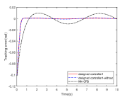
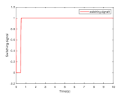
III-F Globally composite neural F-FxT controller with single learning parameter

To further diminish the updating weights, we define $L=\max\left\{{{{\left\|{{l_{i}}}\right\|}^{2}}}\right\},\left({i=1,2,\ldots,n}\right)$.

Then, the virtual control variables ${\alpha_{i}}$ and the control input $u={\alpha_{n}}$ are developed as follows (Method 7-single)

$${\alpha_{1}} =\frac{1}{{{g_{1}}}}\left[{-{k_{1}}{\zeta_{1}}-{k_{12}}\lambda_{1}^{r}+{{\dot{y}}_{r}}-{k_{11}}{\varphi_{1}}\left({{\lambda_{1}}}\right)-{{\hat{d}}_{1}}\tanh\left({\frac{{{\lambda_{1}}}}{{{\eta_{1d}}}}}\right)}\right]$$ (72)

$$-\frac{1}{{{g_{1}}}}\left[{\frac{{{w_{1}}{\lambda_{1}}}}{{2a_{1}^{2}}}{{\hat{L}}}\psi_{1}^{T}{\psi_{1}}+\left({1-{w_{1}}}\right){{\hat{\tau}}_{1}}{H_{1}}\tanh\left({\frac{{{H_{1}}{\lambda_{1}}}}{{{\eta_{1}}}}}\right)}\right]$$

$${\alpha_{i}} =\frac{1}{{{g_{i}}}}\left[{-{k_{i2}}\lambda_{i}^{r}+{{\dot{\rho}}_{i,c}}-{g_{i-1}}{\zeta_{i-1}}-{k_{i1}}{\varphi_{i}}\left({{\lambda_{i}}}\right)-{{\hat{d}}_{i}}\tanh\left({\frac{{{\lambda_{i}}}}{{{\eta_{id}}}}}\right)}\right]$$

$$-\frac{1}{{{g_{i}}}}\left[{k_{i}}{\zeta_{i}}+{\frac{{{w_{i}}{\lambda_{i}}}}{{2a_{i}^{2}}}{{\hat{L}}}\psi_{i}^{T}{\psi_{i}}+\left({1-{w_{i}}}\right){{\hat{\tau}}_{i}}{H_{i}}\tanh\left({\frac{{{H_{i}}{\lambda_{i}}}}{{{\eta_{i}}}}}\right)}\right]$$

where ${\hat{L}},{\hat{\tau}_{i}},{\hat{d}_{i}}$ are the estimation of ${L},{\tau_{i}},{d_{i}}$, respectively, which are as follows

$$\dot{\hat{L}}= {\beta_{h}}\sum\limits_{i=1}^{n}{\frac{{{w_{i}}}}{{2a_{i}^{2}}}\left({\lambda_{i}^{2}+{\beta_{zi}}z_{iN}^{2}}\right)\psi_{i}^{T}{\psi_{i}}}-{\beta_{1}}{\hat{L}^{r}}-{\beta_{2}}{\hat{L}^{m}}$$ (73)

$$-{\beta_{3}}{\hat{L}}$$

$${\dot{\hat{\tau}}_{i}}= {\delta_{i1}}\left({1-{w_{i}}}\right){H_{i}}{\lambda_{i}}\tanh\left({\frac{{{H_{i}}{\lambda_{i}}}}{{{\eta_{i}}}}}\right)-{\delta_{i2}}{{\hat{\tau}}_{i}}^{r}-{\delta_{i3}}\hat{\tau}_{i}^{m}$$

$$-{\delta_{i4}}\hat{\tau}_{i}$$

$${\dot{\hat{d}}_{i}}= {q_{i1}}{\lambda_{i}}\tanh\left({\frac{{{\lambda_{i}}}}{{{\eta_{id}}}}}\right)-{q_{i2}}{{\hat{d}}_{i}}^{r}-{q_{i3}}\hat{d}_{i}^{m}-{q_{i4}}\hat{d}_{i}$$

The prediction errors ${z_{iN}}={\rho_{i}}-{\hat{\rho}_{i}}$ are extracted from the following improved F-FxT SPEM (denote ${\rho_{n+1}}=u$):

$${\dot{\hat{\rho}}_{i}}= \frac{{{w_{i}}\left({{{\bar{\rho}}_{i}}}\right)}}{{2a_{i}^{2}}}{{\hat{L}}}{z_{iN}}\psi_{i}^{T}{\psi_{i}}+\left({1-{w_{i}}}\right){{\hat{\tau}}_{iN}}{H_{i}}\tanh\left({\frac{{{H_{i}}{z_{iN}}}}{{{\eta_{iN}}}}}\right)$$ (74)

$$+{g_{i}}{\rho_{i+1}}+{r_{i1}}z_{iN}^{r}+{r_{i2}}z_{iN}^{m}+{r_{i3}}z_{iN}+{{\hat{d}}_{iN}}\tanh\left({\frac{{{z_{iN}}}}{{{\eta_{idN}}}}}\right)$$

where

$${\dot{\hat{\tau}}_{iN}}= {\delta_{i1N}}\left({1-{w_{i}}}\right){H_{i}}{z_{iN}}\tanh\left({\frac{{{H_{i}}{z_{iN}}}}{{{\eta_{iN}}}}}\right)-{\delta_{i2N}}{{\hat{\tau}}_{iN}}^{r}$$ (75)

$$-{\delta_{i3N}}\hat{\tau}_{iN}^{m}-{\delta_{i4N}}\hat{\tau}_{iN}$$

$${\dot{\hat{d}}_{iN}}= {q_{i1N}}{z_{iN}}\tanh\left({\frac{{{z_{iN}}}}{{{\eta_{idN}}}}}\right)-{q_{i2N}}{{\hat{d}}_{iN}}^{r}-{q_{i3N}}\hat{d}_{iN}^{m}-{q_{i4N}}\hat{d}_{iN}$$

If we define $N=\max\left\{{\max\left\{{{{\bar{\varepsilon}}_{i}},\left\|{{l_{i}}}\right\|}\right\}}\right\},\left({i=1,2,\ldots,n}\right)$ (Method 8-single) or $N=\max\left\{{\left\|{{l_{i}}}\right\|}\right\},\left({i=1,2,\ldots,n}\right)$ (Method 9-single), then another virtual control variables ${\alpha_{i}}$ and the control input $u={\alpha_{n}}$ are constructed as follows

$${\alpha_{1}}=\frac{1}{{{g_{1}}}}\left[{-{k_{1}}{\zeta_{1}}-{k_{12}}\lambda_{1}^{r}+{{\dot{y}}_{r}}-{k_{11}}{\varphi_{1}}\left({{\lambda_{1}}}\right)-{{\hat{d}}_{1}}\tanh\left({\frac{{{\lambda_{1}}}}{{{\eta_{1d}}}}}\right)}\right]$$ (76)

$$-\frac{1}{{{g_{1}}}}\left[{{w_{1}}{{\hat{N}}}{\psi_{1h}}\tanh\left({\frac{{{\psi_{1h}}{\lambda_{1}}}}{{{\eta_{1\theta}}}}}\right)+\left({1-{w_{1}}}\right){{\hat{\tau}}_{1}}{H_{1}}\tanh\left({\frac{{{H_{1}}{\lambda_{1}}}}{{{\eta_{1}}}}}\right)}\right]$$

$${\alpha_{i}}=\frac{1}{{{g_{i}}}}\left[{-{k_{i2}}\lambda_{i}^{r}+{{\dot{\rho}}_{i,c}}-{g_{i-1}}{\zeta_{i-1}}-{k_{i1}}{\varphi_{i}}\left({{\lambda_{i}}}\right)-{{\hat{d}}_{i}}\tanh\left({\frac{{{\lambda_{i}}}}{{{\eta_{id}}}}}\right)}\right]$$

$$-\frac{1}{{{g_{i}}}}\left[{k_{i}}{\zeta_{i}}+{{w_{i}}{{\hat{N}}}{\psi_{ih}}\tanh\left({\frac{{{\psi_{ih}}{\lambda_{i}}}}{{{\eta_{i\theta}}}}}\right)+\left({1-{w_{i}}}\right){{\hat{\tau}}_{i}}{H_{i}}\tanh\left({\frac{{{H_{i}}{\lambda_{i}}}}{{{\eta_{i}}}}}\right)}\right]$$

where ${\hat{N}},{\hat{\tau}_{i}},{\hat{d}_{i}}$ are the estimation of ${N},{\tau_{i}},{d_{i}}$ respectively, which are as follows

$$\dot{\hat{N}}= {\beta_{h}}\sum\limits_{i=1}^{n}{{w_{i}}\left[{{\lambda_{i}}{\psi_{ih}}\tanh\left({\frac{{{\lambda_{i}}{\psi_{ih}}}}{{{\eta_{i\theta}}}}}\right)+{\beta_{zi}}{z_{iN}}{\psi_{ih}}\tanh\left({\frac{{{z_{iN}}{\psi_{ih}}}}{{{\eta_{i\theta N}}}}}\right)}\right]}$$ (77)

$$-{\beta_{1}}{\hat{N}^{r}}-{\beta_{2}}{\hat{N}^{m}}-{\beta_{3}}{\hat{N}}$$

$${\dot{\hat{\tau}}_{i}}= {\delta_{i1}}\left({1-{w_{i}}}\right){H_{i}}{\lambda_{i}}\tanh\left({\frac{{{H_{i}}{\lambda_{i}}}}{{{\eta_{i}}}}}\right)-{\delta_{i2}}{{\hat{\tau}}_{i}}^{r}-{\delta_{i3}}\hat{\tau}_{i}^{m}-{\delta_{i4}}\hat{\tau}_{i}$$

$${\dot{\hat{d}}_{i}}= {q_{i1}}{\lambda_{i}}\tanh\left({\frac{{{\lambda_{i}}}}{{{\eta_{id}}}}}\right)-{q_{i2}}{{\hat{d}}_{i}}^{r}-{q_{i3}}\hat{d}_{i}^{m}-{q_{i4}}\hat{d}_{i}$$

The prediction errors ${z_{iN}}={\rho_{i}}-{\hat{\rho}_{i}}$ are extracted from the following improved F-FxT SPEM (denote ${\rho_{n+1}}=u$):

$${\dot{\hat{\rho}}_{i}}= {w_{i}}{{\hat{N}}}{\psi_{ih}}\tanh\left({\frac{{{\psi_{ih}}{z_{iN}}}}{{{\eta_{i\theta N}}}}}\right)+\left({1-{w_{i}}}\right){{\hat{\tau}}_{iN}}{H_{i}}\tanh\left({\frac{{{H_{i}}{z_{iN}}}}{{{\eta_{iN}}}}}\right)$$ (78)

$$+{g_{i}}{\rho_{i+1}}+{r_{i1}}z_{iN}^{r}+{r_{i2}}z_{iN}^{m}+{r_{i3}}z_{iN}+{{\hat{d}}_{iN}}\tanh\left({\frac{{{z_{iN}}}}{{{\eta_{idN}}}}}\right)$$

where

$${\dot{\hat{\tau}}_{iN}}= {\delta_{i1N}}\left({1-{w_{i}}}\right){H_{i}}{z_{iN}}\tanh\left({\frac{{{H_{i}}{z_{iN}}}}{{{\eta_{iN}}}}}\right)-{\delta_{i2N}}{{\hat{\tau}}_{iN}}^{r}$$ (79)

$$-{\delta_{i3N}}\hat{\tau}_{iN}^{m}-{\delta_{i4N}}\hat{\tau}_{iN}$$

$${\dot{\hat{d}}_{iN}}= {q_{i1N}}{z_{iN}}\tanh\left({\frac{{{z_{iN}}}}{{{\eta_{idN}}}}}\right)-{q_{i2N}}{{\hat{d}}_{iN}}^{r}-{q_{i3N}}\hat{d}_{iN}^{m}-{q_{i4N}}\hat{d}_{iN}$$

Theorem 6

Considering the uncertain strict-feedback system (1), the compensation system (63), the prediction errors and modified F-FxT SPEM (74) or (78), the virtual control law and controller (72) or (76), the adaptive laws (73) or (77), all signals in the closed-loop system are globally F-FxT bounded, and the tracking error tends to an arbitrarily small domain near zero for fast fixed time.

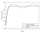
Remark 3

If we set ${H_{i}}\left({{{\bar{\rho}}_{i}}}\right)=1$, the control strategies we designed can be adopted to address the case where the boundaries of the uncertain terms are unknown.

IV Globally composite neural FnT/FxT controllers with input nonlinearities

IV-A Actuator magnitude and rate saturations with known parameters

This section takes Method 4 as an example to illustrate the controller design process under input magnitude and rate (IMR) saturations, which is also applicable to Methods 1 to 9 and Methods 1-single to 9-single.

The IMR saturations are described as $\underline{u}\leq u\leq\bar{u},\underline{\gamma}\leq\dot{u}\leq\bar{\gamma}$. Following [36], the IMR saturations are transformed into the following form

$${\Psi_{\min}}\leq u\leq{\Psi_{\max}}$$ (80)

where ${\Psi_{\min}}=\max\left\{{u\left({t-{T_{r}}}\right)+\underline{\gamma}{T_{r}},\underline{u}}\right\},{\Psi_{\max}}=\min\left\{{u\left({t-{T_{r}}}\right)+\bar{\gamma}{T_{r}},\bar{u}}\right\}$, and $T_{r}>0$ is the sample time.

Then, system (1) subject to IMR saturations is formulated as

$$\left\{\begin{aligned} &{{\dot{\rho}}_{i}}={h_{i}}\left({{{\bar{\rho}}_{i}}}\right)+{g_{i}}\left({{{\bar{\rho}}_{i}}}\right){\rho_{i+1}}+{d_{i}},i=1,2,\ldots,n-1\\ &{{\dot{\rho}}_{n}}={h_{n}}\left({{{\bar{\rho}}_{n}}}\right)+{g_{n}}\left({{{\bar{\rho}}_{n}}}\right)\Psi\left(u\right)+{d_{n}}\\ &y={\rho_{1}}\end{aligned}\right.$$ (81)

where

$$\Psi\left(u\right)=\left\{\begin{aligned} &{\Psi_{\min}},u\leq{\Psi_{\min}}\\ &u,{\Psi_{\min}}\leq u\leq{\Psi_{\max}}\\ &{\Psi_{\max}},u\geq{\Psi_{\max}}\end{aligned}\right.$$ (82)

To work out the known IMR saturations, a novel adaptive F-FxT auxiliary variable system is designed to effectively diminish saturation time, and further alleviate the impact of the auxiliary signal on the tracking error, which is expressed as follows

$$\dot{\Delta}=-{c_{1}}{P_{\Delta}}{\mathop{\rm sig}\nolimits}{\left(\Delta\right)^{{b_{1}}}}-{c_{2}}{P_{\Delta}}{\mathop{\rm sig}\nolimits}{\left(\Delta\right)^{{b_{2}}}}-{c_{3}}{P_{\Delta}}\Delta+{g_{n}}\left({\Psi\left(u\right)-u}\right)$$ (83)

where ${c_{1}}>0,{c_{2}}>0,{c_{3}}>0,0<{b_{1}}<1,{b_{2}}>1$, and ${P_{\Delta}}$ is the adaptive positive gain, which is expressed as

$${\dot{P}_{\Delta}}=\left\{\begin{aligned} &-{k_{p1}}P_{\Delta}^{{{\bar{b}}_{p1}}}-{k_{p2}}P_{\Delta}^{{{\bar{b}}_{p2}}}+{k_{p}}{P^{L}},&\Psi\left(u\right)\neq u\\ &{{\mathop{\rm Proj}\nolimits}_{{P_{\Delta}}}}\left({{k_{p3}}P_{\Delta}^{{b_{3}}}+{k_{p4}}P_{\Delta}^{-{b_{4}}}+{k_{p5}}{P_{\Delta}}+{c_{p}}}\right),&\Psi\left(u\right)=u\end{aligned}\right.$$ (84)

$${{\mathop{\rm Proj}\nolimits}_{{P_{\Delta}}}}\left(\cdot\right)=\left\{\begin{aligned} &0,\left({{P_{\Delta}}={P^{U}},\cdot\geq 0}\right),or\left({{P_{\Delta}}={P^{L}},\cdot\leq 0}\right)\\ &\cdot,otherwise\end{aligned}\right.$$

where ${k_{p}},{k_{p1}},{k_{p2}},{k_{p3}},{k_{p4}},{k_{p5}},{b_{3}},{b_{4}},{c_{p}}$ are positive design parameters, and ${\bar{b}_{p1}}=b_{p1}^{{\mathop{\rm sgn}}\left({{P_{\Delta}}-1}\right)},{\bar{b}_{p2}}=b_{p2}^{{\mathop{\rm sgn}}\left({1-{P_{\Delta}}}\right)},{b_{p1}}>1,0<{b_{p2}}<1$. ${P^{L}}$ and ${P^{U}}$ are the boundaries of ${P_{\Delta}}$

Remark 4

The $\Psi\left(u\right)$ can also be replaced by the smooth function in [36].

The compensation tracking errors are defined as below

$${\lambda_{i}}={\zeta_{i}}-{\sigma_{i}},{\lambda_{n}}={\zeta_{n}}-{\sigma_{n}}-\Delta,i=1,2,\ldots,n-1$$ (85)

Then, the virtual control variables ${\alpha_{i}}$ and the control input $u$ are developed as follows (Method 10)

$${\alpha_{1}} =\frac{1}{{{g_{1}}}}\left[{-{k_{12}}\lambda_{1}^{r}+{{\dot{y}}_{r}}-{k_{11}}{\varphi_{1}}\left({{\lambda_{1}}}\right)-{{\hat{d}}_{1}}\tanh\left({\frac{{{\lambda_{1}}}}{{{\eta_{1d}}}}}\right)}\right]$$ (86)

$$-\frac{1}{{{g_{1}}}}\left[{\frac{{{w_{1}}\left({{{\bar{\rho}}_{1}}}\right){\lambda_{1}}}}{{2a_{1}^{2}}}{{\hat{L}}_{1}}\psi_{1}^{T}{\psi_{1}}+\left({1-{w_{1}}}\right){{\hat{\tau}}_{1}}{H_{1}}\tanh\left({\frac{{{H_{1}}{\lambda_{1}}}}{{{\eta_{1}}}}}\right)}\right],$$

$${\alpha_{i}} =\frac{1}{{{g_{i}}}}\left[{-{k_{i2}}\lambda_{i}^{r}+{{\dot{\rho}}_{i,c}}-{g_{i-1}}{\zeta_{i-1}}-{k_{i1}}{\varphi_{i}}\left({{\lambda_{i}}}\right)-{{\hat{d}}_{i}}\tanh\left({\frac{{{\lambda_{i}}}}{{{\eta_{id}}}}}\right)}\right]$$

$$-\frac{1}{{{g_{i}}}}\left[{\frac{{{w_{i}}\left({{{\bar{\rho}}_{i}}}\right){\lambda_{i}}}}{{2a_{i}^{2}}}{{\hat{L}}_{i}}\psi_{i}^{T}{\psi_{i}}+\left({1-{w_{i}}}\right){{\hat{\tau}}_{i}}{H_{i}}\tanh\left({\frac{{{H_{i}}{\lambda_{i}}}}{{{\eta_{i}}}}}\right)}\right],(i=2,\ldots,n-2),$$

$${\alpha_{i}} =\frac{1}{{{g_{i}}}}\left[{-{k_{i2}}\lambda_{i}^{r}+{{\dot{\rho}}_{i,c}}-{g_{i-1}}{\zeta_{i-1}}-{k_{i1}}{\varphi_{i}}\left({{\lambda_{i}}}\right)-{{\hat{d}}_{i}}\tanh\left({\frac{{{\lambda_{i}}}}{{{\eta_{id}}}}}\right)}\right]$$

$$-\frac{1}{{{g_{i}}}}\left[{\frac{{{w_{i}}\left({{{\bar{\rho}}_{i}}}\right){\lambda_{i}}}}{{2a_{i}^{2}}}{{\hat{L}}_{i}}\psi_{i}^{T}{\psi_{i}}+\left({1-{w_{i}}}\right){{\hat{\tau}}_{i}}{H_{i}}\tanh\left({\frac{{{H_{i}}{\lambda_{i}}}}{{{\eta_{i}}}}}\right)}\right]-\Delta,(i=n-1),$$

$$u =\frac{1}{{{g_{n}}}}\left[{-{k_{n2}}\lambda_{n}^{r}+{{\dot{\rho}}_{n,c}}-{g_{n-1}}{\zeta_{n-1}}-{k_{n1}}{\varphi_{n}}\left({{\lambda_{n}}}\right)-{{\hat{d}}_{n}}\tanh\left({\frac{{{\lambda_{n}}}}{{{\eta_{nd}}}}}\right)}\right]$$

$$-\frac{1}{{{g_{n}}}}\left[{\frac{{{w_{n}}\left({{{\bar{\rho}}_{n}}}\right){\lambda_{n}}}}{{2a_{n}^{2}}}{{\hat{L}}_{n}}\psi_{n}^{T}{\psi_{n}}+\left({1-{w_{n}}}\right){{\hat{\tau}}_{n}}{H_{n}}\tanh\left({\frac{{{H_{n}}{\lambda_{n}}}}{{{\eta_{n}}}}}\right)}\right]$$

$$-\frac{1}{{{g_{n}}}}\left[{{c_{1}}{P_{\Delta}}{\mathop{\rm sig}\nolimits}{{\left(\Delta\right)}^{{b_{1}}}}+{c_{2}}{P_{\Delta}}{\mathop{\rm sig}\nolimits}{{\left(\Delta\right)}^{{b_{2}}}}+{c_{3}}{P_{\Delta}}\Delta}\right],$$

where ${\hat{L}_{i}},{\hat{\tau}_{i}},{\hat{d}_{i}}$ are as follows

$${\dot{\hat{L}}_{i}}={\beta_{hi}}{w_{i}}\left({\lambda_{i}^{2}+{\beta_{zi}}z_{iN}^{2}}\right)\psi_{i}^{T}{\psi_{i}}-{\beta_{i1}}{{\hat{L}}_{i}}^{r}-{\beta_{i2}}\hat{L}_{i}^{m}$$ (87)

$${\dot{\hat{\tau}}_{i}}={\delta_{i1}}\left({1-{w_{i}}}\right){H_{i}}{\lambda_{i}}\tanh\left({\frac{{{H_{i}}{\lambda_{i}}}}{{{\eta_{i}}}}}\right)-{\delta_{i2}}{{\hat{\tau}}_{i}}^{r}-{\delta_{i3}}\hat{\tau}_{i}^{m}$$

$${\dot{\hat{d}}_{i}}={q_{i1}}{\lambda_{i}}\tanh\left({\frac{{{\lambda_{i}}}}{{{\eta_{id}}}}}\right)-{q_{i2}}{{\hat{d}}_{i}}^{r}-{q_{i3}}\hat{d}_{i}^{m}$$

The prediction errors ${z_{iN}}={\rho_{i}}-{\hat{\rho}_{i}}$ are extracted from the following modified FxT SPEM (denote ${\rho_{n+1}}=\Psi\left(u\right)$):

$${\dot{\hat{\rho}}_{i}}= \frac{{{w_{i}}\left({{{\bar{\rho}}_{i}}}\right)}}{{2a_{i}^{2}}}{{\hat{L}}_{i}}{z_{iN}}\psi_{i}^{T}{\psi_{i}}+\left({1-{w_{i}}}\right){{\hat{\tau}}_{iN}}{H_{i}}\tanh\left({\frac{{{H_{i}}{z_{iN}}}}{{{\eta_{iN}}}}}\right)$$ (88)

$$+{g_{i}}{\rho_{i+1}}+{r_{i1}}z_{iN}^{r}+{r_{i2}}z_{iN}^{m}+{{\hat{d}}_{iN}}\tanh\left({\frac{{{z_{iN}}}}{{{\eta_{idN}}}}}\right)$$

where

$${\dot{\hat{\tau}}_{iN}}={\delta_{i1N}}\left({1-{w_{i}}}\right){H_{i}}{z_{iN}}\tanh\left({\frac{{{H_{i}}{z_{iN}}}}{{{\eta_{iN}}}}}\right)-{\delta_{i2N}}{{\hat{\tau}}_{iN}}^{r}-{\delta_{i3N}}\hat{\tau}_{iN}^{m}$$ (89)

$${\dot{\hat{d}}_{iN}}={q_{i1N}}{z_{iN}}\tanh\left({\frac{{{z_{iN}}}}{{{\eta_{idN}}}}}\right)-{q_{i2N}}{{\hat{d}}_{iN}}^{r}-{q_{i3N}}\hat{d}_{iN}^{m}$$

Theorem 7

Considering the system (81) under bounded $u$, the compensation system (39), the adaptive F-FxT auxiliary variable system (83), the prediction errors (88), and the virtual control law and controller (86), all signals in the closed-loop system are globally FxT bounded, and the tracking error tends to an arbitrarily small domain near zero for fixed time.

Remark 5

The developed Method 10 provides a framework for implementing global composite neural FnT/FxT control under IMR saturations, and the auxiliary signal compensators in [33, 34, 35, 36, 37] can also be applied to this.

IV-B Multiple input nonlinearities with unknown parameters

This section takes Method 4 and Method 4-single as examples to illuminate the controller design process under unknown input magnitude saturation, rate saturation and dead-zone simultaneously, which is also applicable to Methods 1 to 9 and Methods 1-single to 9-single.

By adopting (80), the input subject to unknown magnitude saturation, rate saturation and dead-zone is formulated as

$$\Psi\left(u\right)=\left\{\begin{aligned} &{\Psi_{\min}},u\leq{c_{s1}}\\ &{t_{s}}\left(u\right),{c_{s1}}\leq u\leq{c_{s2}}\\ &0,{c_{s2}}\leq u\leq{c_{r1}}\\ &{t_{r}}\left(u\right),{c_{r1}}\leq u\leq{c_{r2}}\\ &{\Psi_{\max}},u\geq{c_{r2}}\end{aligned}\right.$$ (90)

where the assumption of ${t_{s}}\left(u\right),{t_{r}}\left(u\right)$ is the same as [41], and ${c_{s1}}<{c_{s2}}<0,0<{c_{r1}}<{c_{r2}}$ are unknown parameters.

Enlightened by [41], by introducing a smooth function to model the non-smooth actuator nonlinearities, $\Psi\left(u\right)$ can be rewritten as

$$\Psi\left(u\right)={g_{u}}\cdot u+P\left(u\right)$$ (91)

with $0<b<{g_{u}}<\bar{b},\left|{P\left(u\right)}\right|\leq\bar{P}$.

Define tracking errors as follows

$${\zeta_{1}}={\rho_{1}}-{y_{r}}$$ (92)

$${\zeta_{i}}={\rho_{i}}-{\rho_{i,c}},\quad i=2,3,\ldots,n$$

where ${\rho_{i,c}}$ are obtained by the FxT command filter [47] with virtual control variables ${\alpha_{i-1}}$ being inputs.

To alleviate the impact of $\left({{\rho_{i,c}}-{\alpha_{i-1}}}\right)$, the following compensation system is designed

$${{\dot{\sigma}}_{1}}=-{k_{11}}\sigma_{1}^{m}-{k_{12}}\sigma_{1}^{r}+{g_{1}}\left({{\rho_{2,c}}-{\alpha_{1}}}\right)+{g_{1}}{\sigma_{2}}$$ (93)

$${{\dot{\sigma}}_{i}}=-{k_{i1}}\sigma_{i}^{m}-{k_{i2}}\sigma_{i}^{r}+{g_{i}}\left({{\rho_{\left({i+1}\right),c}}-{\alpha_{i}}}\right)-{g_{i-1}}{\sigma_{i-1}}+{g_{i}}{\sigma_{i+1}}$$

$${{\dot{\sigma}}_{n}}=0$$

Then, the virtual control variables ${\alpha_{i}}$ and the control input $u$ are established as (Method 11)

$${\alpha_{1}}=\frac{1}{{{g_{1}}}}\left[{-{k_{12}}\lambda_{1}^{r}+{{\dot{y}}_{r}}-{k_{11}}{\varphi_{1}}\left({{\lambda_{1}}}\right)-{{\hat{d}}_{1}}\tanh\left({\frac{{{\lambda_{1}}}}{{{\eta_{1d}}}}}\right)}\right]$$ (94)

$$-\frac{1}{{{g_{1}}}}\left[{\frac{{{w_{1}}\left({{{\bar{\rho}}_{1}}}\right){\lambda_{1}}}}{{2a_{1}^{2}}}{{\hat{L}}_{1}}\psi_{1}^{T}{\psi_{1}}+\left({1-{w_{1}}}\right){{\hat{\tau}}_{1}}{H_{1}}\tanh\left({\frac{{{H_{1}}{\lambda_{1}}}}{{{\eta_{1}}}}}\right)}\right],$$

$${\alpha_{i}}=\frac{1}{{{g_{i}}}}\left[{-{k_{i2}}\lambda_{i}^{r}+{{\dot{\rho}}_{i,c}}-{g_{i-1}}{\zeta_{i-1}}-{k_{i1}}{\varphi_{i}}\left({{\lambda_{i}}}\right)-{{\hat{d}}_{i}}\tanh\left({\frac{{{\lambda_{i}}}}{{{\eta_{id}}}}}\right)}\right]$$

$$-\frac{1}{{{g_{i}}}}\left[{\frac{{{w_{i}}\left({{{\bar{\rho}}_{i}}}\right){\lambda_{i}}}}{{2a_{i}^{2}}}{{\hat{L}}_{i}}\psi_{i}^{T}{\psi_{i}}+\left({1-{w_{i}}}\right){{\hat{\tau}}_{i}}{H_{i}}\tanh\left({\frac{{{H_{i}}{\lambda_{i}}}}{{{\eta_{i}}}}}\right)}\right],(i=2,\ldots,n-1),$$

$$u=\frac{1}{{{g_{n}}}}\left[{-{k_{n2}}\lambda_{n}^{r}-{k_{n1}}{\varphi_{n}}\left({{\lambda_{n}}}\right)-{{\hat{d}}_{n}}\tanh\left({\frac{{{\lambda_{n}}}}{{{\eta_{nd}}}}}\right)}\right]$$

$$-\frac{1}{{{g_{n}}}}\left[{\frac{{{w_{n}}\left({{{\bar{\rho}}_{n}}}\right){\lambda_{n}}}}{{2a_{n}^{2}}}{{\hat{L}}_{n}}\psi_{n}^{T}{\psi_{n}}+\left({1-{w_{n}}}\right){{\hat{\tau}}_{n}}\tanh\left({\frac{{{\lambda_{n}}}}{{{\eta_{n}}}}}\right)}\right],$$

where ${\hat{L}_{i}},{\hat{\tau}_{i}},{\hat{d}_{i}}$ are as follows

$${\dot{\hat{L}}_{i}}= {\beta_{hi}}{w_{i}}\left({\lambda_{i}^{2}+{\beta_{zi}}z_{iN}^{2}}\right)\psi_{i}^{T}{\psi_{i}}-{\beta_{i1}}{{\hat{L}}_{i}}^{r}$$ (95)

$$-{\beta_{i2}}\hat{L}_{i}^{m},(i=1,\ldots,n-1),$$

$${\dot{\hat{L}}_{n}}= {\beta_{hn}}{w_{u}}{\lambda_{n}^{2}}\psi_{n}^{T}{\psi_{n}}-{\beta_{n1}}{{\hat{L}}_{n}}^{r}-{\beta_{n2}}\hat{L}_{n}^{m},$$

$${\dot{\hat{\tau}}_{i}}= {\delta_{i1}}\left({1-{w_{i}}}\right){H_{i}}{\lambda_{i}}\tanh\left({\frac{{{H_{i}}{\lambda_{i}}}}{{{\eta_{i}}}}}\right)-{\delta_{i2}}{{\hat{\tau}}_{i}}^{r}$$

$$-{\delta_{i3}}\hat{\tau}_{i}^{m},(i=1,\ldots,n-1),$$

$${\dot{\hat{\tau}}_{n}}= {\delta_{n1}}\left({1-{w_{n}}}\right){\lambda_{n}}\tanh\left({\frac{{{\lambda_{n}}}}{{{\eta_{n}}}}}\right)-{\delta_{n2}}{{\hat{\tau}}_{n}}^{r}-{\delta_{n3}}\hat{\tau}_{n}^{m}$$

$${\dot{\hat{d}}_{i}}= {q_{i1}}{\lambda_{i}}\tanh\left({\frac{{{\lambda_{i}}}}{{{\eta_{id}}}}}\right)-{q_{i2}}{{\hat{d}}_{i}}^{r}-{q_{i3}}\hat{d}_{i}^{m}$$

The prediction errors ${z_{iN}}={\rho_{i}}-{\hat{\rho}_{i}},(i=1,\ldots,n-1)$ are extracted from the following modified FxT SPEM:

$${\dot{\hat{\rho}}_{i}}= \frac{{{w_{i}}\left({{{\bar{\rho}}_{i}}}\right)}}{{2a_{i}^{2}}}{{\hat{L}}_{i}}{z_{iN}}\psi_{i}^{T}{\psi_{i}}+\left({1-{w_{i}}}\right){{\hat{\tau}}_{iN}}{H_{i}}\tanh\left({\frac{{{H_{i}}{z_{iN}}}}{{{\eta_{iN}}}}}\right)$$ (96)

$$+{g_{i}}{\rho_{i+1}}+{r_{i1}}z_{iN}^{r}+{r_{i2}}z_{iN}^{m}+{{\hat{d}}_{iN}}\tanh\left({\frac{{{z_{iN}}}}{{{\eta_{idN}}}}}\right)$$

where

$${\dot{\hat{\tau}}_{iN}}={\delta_{i1N}}\left({1-{w_{i}}}\right){H_{i}}{z_{iN}}\tanh\left({\frac{{{H_{i}}{z_{iN}}}}{{{\eta_{iN}}}}}\right)-{\delta_{i2N}}{{\hat{\tau}}_{iN}}^{r}-{\delta_{i3N}}\hat{\tau}_{iN}^{m}$$ (97)

$${\dot{\hat{d}}_{iN}}={q_{i1N}}{z_{iN}}\tanh\left({\frac{{{z_{iN}}}}{{{\eta_{idN}}}}}\right)-{q_{i2N}}{{\hat{d}}_{iN}}^{r}-{q_{i3N}}\hat{d}_{iN}^{m}$$

To further decline the updating weights, we define $L=\max\left\{{{{\left\|{{l_{i}}}\right\|}^{2}}}\right\},\left({i=1,2,\ldots,n-1}\right)$.

Then, the virtual control variables ${\alpha_{i}}$ and the control input $u$ are developed as follows (Method 12)

$${\alpha_{1}}=\frac{1}{{{g_{1}}}}\left[{-{k_{12}}\lambda_{1}^{r}+{{\dot{y}}_{r}}-{k_{11}}{\varphi_{1}}\left({{\lambda_{1}}}\right)-{{\hat{d}}_{1}}\tanh\left({\frac{{{\lambda_{1}}}}{{{\eta_{1d}}}}}\right)}\right]$$ (98)

$$-\frac{1}{{{g_{1}}}}\left[{\frac{{{w_{1}}{\lambda_{1}}}}{{2a_{1}^{2}}}{{\hat{L}}}\psi_{1}^{T}{\psi_{1}}+\left({1-{w_{1}}}\right){{\hat{\tau}}_{1}}{H_{1}}\tanh\left({\frac{{{H_{1}}{\lambda_{1}}}}{{{\eta_{1}}}}}\right)}\right]$$

$${\alpha_{i}}=\frac{1}{{{g_{i}}}}\left[{-{k_{i2}}\lambda_{i}^{r}+{{\dot{\rho}}_{i,c}}-{g_{i-1}}{\zeta_{i-1}}-{k_{i1}}{\varphi_{i}}\left({{\lambda_{i}}}\right)-{{\hat{d}}_{i}}\tanh\left({\frac{{{\lambda_{i}}}}{{{\eta_{id}}}}}\right)}\right]$$

$$-\frac{1}{{{g_{i}}}}\left[{\frac{{{w_{i}}{\lambda_{i}}}}{{2a_{i}^{2}}}{{\hat{L}}}\psi_{i}^{T}{\psi_{i}}+\left({1-{w_{i}}}\right){{\hat{\tau}}_{i}}{H_{i}}\tanh\left({\frac{{{H_{i}}{\lambda_{i}}}}{{{\eta_{i}}}}}\right)}\right],(i=2,\ldots,n-1),$$

$$u=\frac{1}{{{g_{n}}}}\left[{-{k_{n2}}\lambda_{n}^{r}-{k_{n1}}{\varphi_{n}}\left({{\lambda_{n}}}\right)-{{\hat{d}}_{n}}\tanh\left({\frac{{{\lambda_{n}}}}{{{\eta_{nd}}}}}\right)}\right]$$

$$-\frac{1}{{{g_{n}}}}\left[{\frac{{{w_{n}}\left({{{\bar{\rho}}_{n}}}\right){\lambda_{n}}}}{{2a_{n}^{2}}}{{\hat{L}}_{u}}\psi_{n}^{T}{\psi_{n}}+\left({1-{w_{n}}}\right){{\hat{\tau}}_{n}}\tanh\left({\frac{{{\lambda_{n}}}}{{{\eta_{n}}}}}\right)}\right],$$

where ${\hat{L}},{\hat{\tau}_{i}},{\hat{d}_{i}}$ are as follows

$$\dot{\hat{L}}= {\beta_{h}}\sum\limits_{i=1}^{n-1}{\frac{{{w_{i}}}}{{2a_{i}^{2}}}\left({\lambda_{i}^{2}+{\beta_{zi}}z_{iN}^{2}}\right)\psi_{i}^{T}{\psi_{i}}}-{\beta_{1}}{\hat{L}^{r}}-{\beta_{2}}{\hat{L}^{m}}$$ (99)

$${\dot{\hat{L}}_{u}}= {\beta_{hn}}{w_{u}}{\lambda_{n}^{2}}\psi_{n}^{T}{\psi_{n}}-{\beta_{n1}}{{\hat{L}}_{u}}^{r}-{\beta_{n2}}\hat{L}_{u}^{m}$$

$${\dot{\hat{\tau}}_{i}}= {\delta_{i1}}\left({1-{w_{i}}}\right){H_{i}}{\lambda_{i}}\tanh\left({\frac{{{H_{i}}{\lambda_{i}}}}{{{\eta_{i}}}}}\right)-{\delta_{i2}}{{\hat{\tau}}_{i}}^{r}$$

$$-{\delta_{i3}}\hat{\tau}_{i}^{m},(i=1,\ldots,n-1),$$

$${\dot{\hat{\tau}}_{n}}= {\delta_{n1}}\left({1-{w_{n}}}\right){\lambda_{n}}\tanh\left({\frac{{{\lambda_{n}}}}{{{\eta_{n}}}}}\right)-{\delta_{n2}}{{\hat{\tau}}_{n}}^{r}-{\delta_{n3}}\hat{\tau}_{n}^{m}$$

$${\dot{\hat{d}}_{i}}= {q_{i1}}{\lambda_{i}}\tanh\left({\frac{{{\lambda_{i}}}}{{{\eta_{id}}}}}\right)-{q_{i2}}{{\hat{d}}_{i}}^{r}-{q_{i3}}\hat{d}_{i}^{m}$$

The prediction errors ${z_{iN}}={\rho_{i}}-{\hat{\rho}_{i}},(i=1,\ldots,n-1)$ are extracted from the following improved fixed-time SPEM:

$${\dot{\hat{\rho}}_{i}}= \frac{{{w_{i}}\left({{{\bar{\rho}}_{i}}}\right)}}{{2a_{i}^{2}}}{{\hat{L}}}{z_{iN}}\psi_{i}^{T}{\psi_{i}}+\left({1-{w_{i}}}\right){{\hat{\tau}}_{iN}}{H_{i}}\tanh\left({\frac{{{H_{i}}{z_{iN}}}}{{{\eta_{iN}}}}}\right)$$ (100)

$$+{g_{i}}{\rho_{i+1}}+{r_{i1}}z_{iN}^{r}+{r_{i2}}z_{iN}^{m}+{{\hat{d}}_{iN}}\tanh\left({\frac{{{z_{iN}}}}{{{\eta_{idN}}}}}\right)$$

where

$${\dot{\hat{\tau}}_{iN}}={\delta_{i1N}}\left({1-{w_{i}}}\right){H_{i}}{z_{iN}}\tanh\left({\frac{{{H_{i}}{z_{iN}}}}{{{\eta_{iN}}}}}\right)-{\delta_{i2N}}{{\hat{\tau}}_{iN}}^{r}-{\delta_{i3N}}\hat{\tau}_{iN}^{m}$$ (101)

$${\dot{\hat{d}}_{iN}}={q_{i1N}}{z_{iN}}\tanh\left({\frac{{{z_{iN}}}}{{{\eta_{idN}}}}}\right)-{q_{i2N}}{{\hat{d}}_{iN}}^{r}-{q_{i3N}}\hat{d}_{iN}^{m}$$

Theorem 8

Considering the system (81) subject to (90), the compensation system (93), the prediction errors (96) or (100), the virtual control law and controller (94) or (98), all signals in the closed-loop system are globally FxT bounded, and the tracking error tends to an arbitrarily small domain near zero for fixed time.

Remark 6

The established Method 11 and Method 12 can also be applied to achieve global composite neural FnT/FxT control under both input saturation and dead-zone, IMR saturations, or single input nonlinearity.

(a) Tracking errors

(b) Switching signal

Figure 1: Results of Method 1

(a) Tracking errors

(b) Switching signal

Figure 2: Results of Method 2

(a) Tracking errors

(b) Switching signal

Figure 3: Results of Method 3

(a) Tracking errors

(b) Switching signal

Figure 4: Results of Method 4

(a) Tracking errors

(b) Switching signal

Figure 5: Results of Method 5

(a) Tracking errors

(b) Switching signal

Figure 6: Results of Method 6

V Simulation Results

In this section, the following inverted pendulum model [49] is employed to evince validity of the designed control strategies:

$${{\dot{\rho}}_{1}}={\rho_{2}}$$ (102)

$${{\dot{\rho}}_{2}}=\frac{{{g_{e}}\sin{\rho_{1}}-\frac{{{m_{a}}{l_{a}}\rho_{2}^{2}\cos{\rho_{1}}\sin{\rho_{1}}}}{{{m_{c}}+{m_{a}}}}}}{{{l_{a}}\left({\frac{4}{3}-\frac{{{m_{a}}{{\cos}^{2}}{\rho_{1}}}}{{{m_{c}}+{m_{a}}}}}\right)}}+\frac{{\frac{{\cos{\rho_{1}}}}{{{m_{c}}+{m_{a}}}}}}{{{l_{a}}\left({\frac{4}{3}-\frac{{{m_{a}}{{\cos}^{2}}{\rho_{1}}}}{{{m_{c}}+{m_{a}}}}}\right)}}u+{d_{2}}$$

where $g_{e}=9.81\,{\rm{}}{{\rm{m}}\mathord{\left/{\vphantom{{\rm{m}}{{{\rm{s}}^{2}}}}}\right.\kern-1.2pt}{{{\rm{s}}^{2}}}}$, ${m_{c}}=1\,{\rm{kg}}$, ${m_{a}}=0.1\,{\rm{kg}}$, ${l_{a}}=0.5\,{\rm{m}}$, and ${\rho_{1}}\left(0\right)=-0.1\,{\rm{rad}}$. $y_{r}=0.2\sin(t)\,{\rm{rad}}$.

The parameters of designed FnT controllers are set as ${k_{1}}=2,{k_{2}}=4,m=0.6,{p_{1}}={p_{2}}=0.5,{\gamma_{1}}={\gamma_{2}}=1,{a_{2}}=1,{\beta_{h2}}=10,{\delta_{21}}={\delta_{21N}}=10$, and the parameters of designed FxT controllers are selected as ${k_{11}}={k_{21}}=2,{k_{12}}={k_{22}}=4,r=5/3,{a_{2}}=1,{\beta_{h2}}=10,{\delta_{21}}={\delta_{21N}}=10$. The RBFNN embodies 121 nodes with centers distributed evenly in $\left[{-0.25,0.25}\right]\times\left[{-0.25,0.25}\right]$ and widths are chosen as $2$. The designed controller without composite adaptive laws and the NN-based command-filtered backstepping algorithm [5] are adopted as the comparison approaches, labeled as designed controller-without and NN-CFB, respectively.

The simulation results displayed in Fig. 1-6 (a) manifest that the tracking performance is enhanced via the developed composite learning approaches, and the presented composite FnT/FxT controllers possess faster transient responses. Moreover, the switching signals depicted in Fig. 1-6 (b) reveal that the constructed robust control law has the capability to drive external transients back into the RBFNN’s valid domain to ensure the global stability of the designed control strategies.

VI Conclusion

In this article, globally composite adaptive law-based intelligent FnT/FxT control strategies have been developed to cope with the tracking control issue for a class of uncertain strict-feedback nonlinear systems. RBFNNs with novel composite updating weights are constructed to boost tracking performance and decline the NNs’ learning parameters simultaneously. By virtue of a newly designed switching mechanism, system states can be brought back when they transcend the neural working region. A modified FnT/FxT backstepping algorithm is established to steer output to track the reference signal. A novel adaptive F-FxT auxiliary variable system is designed to cope with the input issue under known magnitude and rate saturations. For the input subject to unknown magnitude saturation, rate saturation and dead-zone simultaneously, a smooth function is introduced to model the non-smooth actuator nonlinearities, and the unknown parameters are approximated by adopting the proposed global RBFNNs. Stability analysis illuminates that the tracking error tends to an arbitrarily small residual set for finite/fixed time, while all signals in the closed-loop system are globally FnT/FxT bounded. A simulation example elucidates the validity of theoretical results.

References

• [1] D. Swaroop, J. Hedrick, P. Yip, and J. Gerdes, “Dynamic surface control for a class of nonlinear systems,” IEEE Transactions on Automatic Control, vol. 45, no. 10, pp. 1893–1899, 2000.
• [2] J. A. Farrell, M. Polycarpou, M. Sharma, and W. Dong, “Command filtered backstepping,” IEEE Transactions on Automatic Control, vol. 54, no. 6, pp. 1391–1395, 2009.
• [3] W. Dong, J. A. Farrell, M. M. Polycarpou, V. Djapic, and M. Sharma, “Command filtered adaptive backstepping,” IEEE Transactions on Control Systems Technology, vol. 20, no. 3, pp. 566–580, 2012.
• [4] D. Wang and J. Huang, “Neural network-based adaptive dynamic surface control for a class of uncertain nonlinear systems in strict-feedback form,” IEEE Transactions on Neural Networks, vol. 16, no. 1, pp. 195–202, 2005.
• [5] C. Li and X. Yang, “Neural networks-based command filtering control for a table-mount experimental helicopter,” Journal of the Franklin Institute, vol. 358, no. 1, pp. 321–338, 2021.
• [6] D. Gao, Z. Sun, and T. Du, “Dynamic surface control for hypersonic aircraft using fuzzy logic system,” in 2007 IEEE International Conference on Automation and Logistics, pp. 2314–2319, 2007.
• [7] S. Tong and Y. Li, “Adaptive fuzzy output feedback tracking backstepping control of strict-feedback nonlinear systems with unknown dead zones,” IEEE Transactions on Fuzzy Systems, vol. 20, no. 1, pp. 168–180, 2012.
• [8] B. Xu, Z. Shi, C. Yang, and F. Sun, “Composite neural dynamic surface control of a class of uncertain nonlinear systems in strict-feedback form,” IEEE Transactions on Cybernetics, vol. 44, no. 12, pp. 2626–2634, 2014.
• [9] G. Zhang, S. Chu, X. Jin, and W. Zhang, “Composite neural learning fault-tolerant control for underactuated vehicles with event-triggered input,” IEEE Transactions on Cybernetics, vol. 51, no. 5, pp. 2327–2338, 2021.
• [10] Y. Cheng, B. Xu, Z. Lian, Z. Shi, and P. Shi, “Adaptive learning control of switched strict-feedback nonlinear systems with dead zone using NN and DOB,” IEEE Transactions on Neural Networks and Learning Systems, pp. 1–10, 2021.
• [11] J.-T. Huang, “Global tracking control of strict-feedback systems using neural networks,” IEEE Transactions on Neural Networks and Learning Systems, vol. 23, no. 11, pp. 1714–1725, 2012.
• [12] C. Yang, Y. Jiang, Z. Li, W. He, and C.-Y. Su, “Neural control of bimanual robots with guaranteed global stability and motion precision,” IEEE Transactions on Industrial Informatics, vol. 13, no. 3, pp. 1162–1171, 2017.
• [13] B. Xu, X. Wang, F. Sun, and Z. Shi, “Intelligent control of flexible hypersonic flight dynamics with input dead zone using singular perturbation decomposition,” IEEE Transactions on Neural Networks and Learning Systems, pp. 1–11, 2021.
• [14] B. Xu, X. Wang, W. Chen, and P. Shi, “Robust intelligent control of SISO nonlinear systems using switching mechanism,” IEEE Transactions on Cybernetics, vol. 51, no. 8, pp. 3975–3987, 2021.
• [15] H. Wang, Y. Tian, and H. Xu, “Neural adaptive command filtered control for cooperative path following of multiple underactuated autonomous underwater vehicles along one path,” IEEE Transactions on Systems, Man, and Cybernetics: Systems, vol. 52, no. 5, pp. 2966–2978, 2022.
• [16] Q. Wang, Z. Zhang, and X.-J. Xie, “Globally adaptive neural network tracking for uncertain output-feedback systems,” IEEE Transactions on Neural Networks and Learning Systems, vol. 34, no. 2, pp. 814–823, 2023.
• [17] J. Yu, P. Shi, and L. Zhao, “Finite-time command filtered backstepping control for a class of nonlinear systems,” Automatica, vol. 92, pp. 173–180, 2018.
• [18] Y.-X. Li, “Finite time command filtered adaptive fault tolerant control for a class of uncertain nonlinear systems,” Automatica, vol. 106, pp. 117–123, 2019.
• [19] L. Zhao, G. Liu, and J. Yu, “Finite-time adaptive fuzzy tracking control for a class of nonlinear systems with full-state constraints,” IEEE Transactions on Fuzzy Systems, vol. 29, no. 8, pp. 2246–2255, 2021.
• [20] L. Zhao, J. Yu, and Q.-G. Wang, “Finite-time tracking control for nonlinear systems via adaptive neural output feedback and command filtered backstepping,” IEEE Transactions on Neural Networks and Learning Systems, vol. 32, no. 4, pp. 1474–1485, 2021.
• [21] X. Wang and B. Xu, “Robust adaptive control of hypersonic flight vehicle with aero-servo-elastic effect,” IEEE Transactions on Aerospace and Electronic Systems, pp. 1–10, 2022.
• [22] X. Wang, Z. Li, X. Yu, and Z. He, “Adaptive smooth disturbance observer-based fast finite-time attitude tracking control of a small unmanned helicopter,” Journal of the Franklin Institute, vol. 359, no. 11, pp. 5322–5340, 2022.
• [23] J. Ni and P. Shi, “Adaptive neural network fixed-time leader-follower consensus for multiagent systems with constraints and disturbances,” IEEE Transactions on Cybernetics, vol. 51, no. 4, pp. 1835–1848, 2021.
• [24] X. Yuan, B. Chen, and C. Lin, “Neural adaptive fixed-time control for nonlinear systems with full-state constraints,” IEEE Transactions on Cybernetics, pp. 1–12, 2021.
• [25] G. Cui, W. Yang, J. Yu, Z. Li, and C. Tao, “Fixed-time prescribed performance adaptive trajectory tracking control for a QUAV,” IEEE Transactions on Circuits and Systems II: Express Briefs, vol. 69, no. 2, pp. 494–498, 2022.
• [26] L. Zhang, B. Chen, C. Lin, and Y. Shang, “Fuzzy adaptive fixed-time consensus tracking control of high-order multiagent systems,” IEEE Transactions on Fuzzy Systems, vol. 30, no. 2, pp. 567–578, 2022.
• [27] A. Polyakov, “Nonlinear feedback design for fixed-time stabilization of linear control systems,” IEEE Transactions on Automatic Control, vol. 57, no. 8, pp. 2106–2110, 2012.
• [28] F. Wang and G. Lai, “Fixed-time control design for nonlinear uncertain systems via adaptive method,” Systems & Control Letters, vol. 140, p. 104704, 2020.
• [29] B. Xin, S. Cheng, Q. Wang, J. Chen, and F. Deng, “Fixed-time prescribed performance consensus control for multi-agent systems with non-affine faults,” IEEE Transactions on Fuzzy Systems, pp. 1–14, 2023.
• [30] J. Sun, H. He, J. Yi, and Z. Pu, “Finite-time command-filtered composite adaptive neural control of uncertain nonlinear systems,” IEEE Transactions on Cybernetics, vol. 52, no. 7, pp. 6809–6821, 2022.
• [31] B. Xu, X. Wang, Y. Shou, P. Shi, and Z. Shi, “Finite-time robust intelligent control of strict-feedback nonlinear systems with flight dynamics application,” IEEE Transactions on Neural Networks and Learning Systems, vol. 33, no. 11, pp. 6173–6182, 2022.
• [32] Z. Wu, S. Zheng, Y. Zhao, B. Liu, and J. Ni, “Fixed-time composite neural learning control of state-constrained nonlinear uncertain systems,” Journal of the Franklin Institute, vol. 358, no. 16, pp. 8138–8168, 2021.
• [33] X. Bu, X. Wu, D. Wei, and J. Huang, “Neural-approximation-based robust adaptive control of flexible air-breathing hypersonic vehicles with parametric uncertainties and control input constraints,” Information Sciences, vol. 346, pp. 29–43, 2016.
• [34] W. Sun, S. Diao, S.-F. Su, and Z.-Y. Sun, “Fixed-time adaptive neural network control for nonlinear systems with input saturation,” IEEE Transactions on Neural Networks and Learning Systems, vol. 34, no. 4, pp. 1911–1920, 2023.
• [35] Y. Ding, X. Wang, Y. Bai, and N. Cui, “Novel anti-saturation robust controller for flexible air-breathing hypersonic vehicle with actuator constraints,” ISA transactions, vol. 99, pp. 95–109, 2020.
• [36] J. Sun, J. Yi, and Z. Pu, “Fixed-time adaptive fuzzy control for uncertain nonstrict-feedback systems with time-varying constraints and input saturations,” IEEE Transactions on Fuzzy Systems, vol. 30, no. 4, pp. 1114–1128, 2022.
• [37] Y. Ding, X. Yue, C. Liu, H. Dai, and G. Chen, “Finite-time controller design with adaptive fixed-time anti-saturation compensator for hypersonic vehicle,” ISA transactions, vol. 122, pp. 96–113, 2022.
• [38] Y. Li, S. Tong, and T. Li, “Composite adaptive fuzzy output feedback control design for uncertain nonlinear strict-feedback systems with input saturation,” IEEE Transactions on Cybernetics, vol. 45, DOI 10.1109/TCYB.2014.2370645, no. 10, pp. 2299–2308, 2015.
• [39] L. Zhang, W.-W. Che, S. Xu, and C. Deng, “Prescribed performance tracking control for 2-d plane vehicle platoons with actuator faults and saturations,” IEEE Transactions on Vehicular Technology, pp. 1–11, 2023.
• [40] X. Zhou, C. Gao, Z.-g. Li, X.-y. Ouyang, and L.-b. Wu, “Observer-based adaptive fuzzy finite-time prescribed performance tracking control for strict-feedback systems with input dead-zone and saturation,” Nonlinear Dynamics, vol. 103, pp. 1645–1661, 2021.
• [41] S. Kang, P. X. Liu, and H. Wang, “Fixed-time adaptive fuzzy command filtering control for a class of uncertain nonlinear systems with input saturation and dead zone,” Nonlinear Dynamics, vol. 110, no. 3, pp. 2401–2414, 2022.
• [42] M. M. Polycarpou and P. A. Ioannou, “A robust adaptive nonlinear control design,” Automatica, vol. 32, no. 3, pp. 423–427, 1996.
• [43] C. Qian and W. Lin, “A continuous feedback approach to global strong stabilization of nonlinear systems,” IEEE Transactions on Automatic Control, vol. 46, no. 7, pp. 1061–1079, 2001.
• [44] A. Abdurahman, H. Jiang, and C. Hu, “Improved fixed-time stability results and application to synchronization of discontinuous neural networks with state-dependent switching,” International Journal of Robust and Nonlinear Control, vol. 31, no. 12, pp. 5725–5744, 2021.
• [45] X. Wang and B. Shirinzadeh, “Rapid-convergent nonlinear differentiator,” Mechanical Systems and Signal Processing, vol. 28, pp. 414–431, 2012.
• [46] J. Park and I. Sandberg, “Universal approximation using radial-basis-function networks,” Neural Computation, vol. 3, no. 2, pp. 246–257, 2014.
• [47] E. Cruz Zavala, J. A. Moreno, and L. M. Fridman, “Uniform robust exact differentiator,” IEEE Transactions on Automatic Control, vol. 56, no. 11, pp. 2727–2733, 2011.
• [48] X. Wang, Z. Li, Z. He, and M. V. Basin, “Prescribed performance adaptive tracking control with small overshoot for a class of uncertain second-order nonlinear systems,” IEEE Transactions on Circuits and Systems II: Express Briefs, vol. 69, no. 9, pp. 3834–3838, 2022.
• [49] J.-X. Zhang and G.-H. Yang, “Prescribed performance fault-tolerant control of uncertain nonlinear systems with unknown control directions,” IEEE Transactions on Automatic Control, vol. 62, no. 12, pp. 6529–6535, 2017.