Searching for long faint astronomical high energy transients: a data driven approach

Abstract

HERMES (High Energy Rapid Modular Ensemble of Satellites) pathfinder is an in-orbit demonstration consisting of a constellation of six 3U nano-satellites hosting simple but innovative detectors for the monitoring of cosmic high-energy transients. The main objective of HERMES Pathfinder is to prove that accurate position of high-energy cosmic transients can be obtained using miniaturized hardware. The transient position is obtained by studying the delay time of arrival of the signal to different detectors hosted by nano-satellites on low Earth orbits. To this purpose, particular attention is placed on optimizing the time accuracy, with the goal of reaching an overall accuracy of a fraction of a micro-second. In this context, we need to develop novel tools to fully exploit the future scientific data output of HERMES Pathfinder. In this paper, we introduce a new framework to assess the background count rate of a space-born, high energy detector; a key step towards the identification of faint astrophysical transients. We employ a Neural Network (NN) to estimate the background lightcurves on different timescales. Subsequently, we employ a fast change-point and anomaly detection technique to isolate observation segments where statistically significant excesses in the observed count rate relative to the background estimate exist. We test the new software on archival data from the NASA Fermi Gamma-ray Burst Monitor (GBM), which has a collecting area and background level of the same order of magnitude to those of HERMES Pathfinder. The neural network performances are discussed and analyzed over period of both high and low solar activity. We were able to confirm events in the Fermi/GBM catalog, both Solar Flares and Gamma-Ray Bursts (GRBs), and found events, not present in Fermi/GBM database, that could be attributed to Solar Flares, Terrestrial Gamma-ray Flashes, GRBs, Galactic X-ray flash. Seven of these are selected and analyzed further, providing an estimate of localisation and a tentative classification.

1 Introduction

Gamma-Ray Bursts (GRBs) originate in extraordinarily energetic explosions taking place in distant galaxies. They appear as irregular pulses of X and $\gamma$-ray radiation in detectors of today work-horse satellites such as SWIFT, INTEGRAL, Fermi, and Agile. The typical distribution of GRBs duration is bimodal; ‘long bursts’, lasting longer than 2s, are associated with black hole formation in collapsars, while ‘short bursts’, lasting less than 2s, are associated to mergers of binary neutron stars Woosley (1993); Berger (2014).

Present instrumentation dedicated to GRBs and cosmic transients has been launched during the 2010s. There is no guarantee that it will continue to operate beyond the mid-2020s. For this reason, several proposals to NASA and ESA have been already submitted to select the successors of these instruments. The High Energy Rapid Modular Ensemble of Satellites (HERMES) concept is to develop a constellation of nano-satellites to study high-energy transients Fiore et al. (2020, 2021), thus providing a fast-track and affordable solution bridging the gap between current X-ray monitors and the next generation. A technological and scientific pathfinder (HERMES-TP, funded by ASI and HERMES-SP funded by the European Commission, HERMES pathfinder hereafter) is in preparation to prove the concept, that is the capability to detect and localize GRBs with miniaturized instrumentation hosted by nano-satellites. The first six HERMES Pathfinder spacecrafts are expected to be launched in low-Earth, near-equatorial orbit during 2024. A seventh payload unit identical to those hosted by HERMES Pathfinder is also hosted by the Australian SpiRIT satellite, to be launched during 2023. The HERMES Pathfinder and SpIRIT payload is a small yet innovative “siswich" detector providing broad-band energy coverage (few keV - $1$ MeV) and very good temporal resolution (a few hundreds ns) Fuschino et al. (2019); Evangelista et al. (2020); Fiore et al. (2022); Evangelista et al. (2022).

GRBs manifest as transient increases in the count rates of detectors. The activity of these phenomena appear as unexpected, and not explainable in terms of background or any other known sources. Any automated procedure for detecting GRBs is generally concerned with searching the time series of the observations for statistically significant excesses in photon counts, relative to a reference background estimate in the absence of $\gamma$/X-ray GRB related events. The on-orbit physical background observed by GRB monitor experiments is determined by factors inherent to the highly dynamical near-Earth radiation environment, to the spacecraft geographic position and attitude, as well as the spacecraft geometry, and the detector’s pointing, design and response. Given the difficulty intrinsic to a real-time modelling of the expected scientific background, algorithms dedicated to the ‘online’ search of GRBs often resort to extrapolate the background from recent observations. For example, the trigger algorithms running on-board NASA Fermi/GBM assess a background estimate from an average of the photon count rate observed over the previous $17$ s excluding the most recent $4$ s of observations Meegan et al. (2009); similar moving average approaches were used by Compton-BATSE Paciesas et al. (1999) and BeppoSAX-GRBM Feroci et al. (1997).

In ‘offline’ analysis, archival data are searched for GRB events that the online and on-board algorithms may have missed. Examples of this approach can be found in Kommers (1999), which uses the BATSE catalog, or in Kocevski et al. (2018) and Hui et al. (2017) where they search for faint, short GRBs at times compatible with known gravitational wave events. In Biltzinger et al. (2020) for example, an estimate is assessed starting from detailed models of the background expected for GBM, such as the detector response, the cosmic $\gamma$-ray background, the solar activity, the geomagnetic environment, the Earth albedo and the visibility of X and $\gamma$ point sources. The background description so achieved has been shown to reproduce very well the observations of Fermi/GBM and could potentially allow for the identification of otherwise hard to detect GRBs such as long-weak events with slow raising times. However, having been specifically tailored for the observations of Fermi/GBM, this technique is not immediately applicable to other experiments. In Sadeh (2019) a Recurrent Neural Network (RNN LeCun et al. (2015)) is used to predict the background and, on top of it, classify or detect anomalies in the observations of a count-rate detector. To recognize a GRB event, this RNN is trained onto existing catalogues of burst observations. We believe such an approach could inherit the detection biases of standard strategies for GRB detection, ultimately leading to missing events which already defied previous searches.

In Section 2 we introduce our approach to estimate the scientific background of a gamma-ray burst monitor experiment using a Neural Network (NN). In particular, we employ a Feed Forward Neural Network (Bishop et al. (1995)) to estimate the count-rates expected from background sources over the 12 NaI detectors of Fermi/GBM, in different energy bands and at regular time intervals. Our model is designed to learn the dynamics of the background over a timescale of months, enabling the detection of long-GRBs or even ultralong-GRBs Gendre et al. (2019), as shown in an example in Section A. Moreover, employing a robust loss function in the training phase, we are able to deal with outliers in count-rate observations, such as transients due to astronomical events or brief period of detector inactivity C. The choice of applying our framework to archival data from Fermi was motivated by the facts that (1) the HERMES Pathfinder spacecrafts are expected to be launched in a low inclination orbit with altitude $500-550$ km, an orbit where the background and its variations are expected to be smaller than those of Fermi/GBM Meegan et al. (2009); and (2) the Fermi/GBM and HERMES Pathfinder detectors both rely onto scintillators and have similar effective areas Bissaldi et al. (2009); Campana et al. (2020); Dilillo et al. (2022) resulting in background count-rates of the same order of magnitude. To estimate the background observed by Fermi/GBM, we leverage on a large ensemble of information, including features both intrinsic to the satellite and its orbital setting such as the satellite attitude and geographic location in time, the Sun visibility and so on. This idea is consistent with Fitzpatrick et al. (2012), which describes a method that estimates the background at the period of interest by using rates from adjacent days when the satellite has similar geographical footprint. To retrieve these information’s we use the Fermi/GBM Data Tools Goldstein et al. (2021) software package, an Application Programming Interface (API) allowing to download, analyse and visualise GBM data. Being completely data-driven, we believe our approach to be in principle applicable to any GRB monitor experiment for which a similar dataset is available.

The background estimates produced by the NN are compared with the observations by mean of an efficient change-point detection technique called FOCuS-Poisson Ward et al. (2022), aiming at the automatic identification of statistically significant astrophysical transients. We tested the combination of the NN background estimates and FOCuS-Poisson trigger on real Fermi/GBM data. We were able to confirm known events, but we also find events with no counterpart in the Fermi/GBM trigger catalog (Von Kienlin et al., 2020), yet with features resembling astronomical transients such as GRBs and solar flares and other galactic high-energy sources.

The paper is organised as follows. In Section 2 we present the background estimation in a supervised Machine Learning settings, the architecture of the NN and the FOCuS-Poisson change-point detection technique. In Section 3 we describe the data used and the pre-processing steps to build the dataset. In Section 4 we report the performance of the NN estimator and the result of the application of the trigger algorithm. A comparison between the background estimated in a period of solar maxima and in a solar minima is described in the Appendix C. In Section 5 we discuss the results of our search for undiscovered astrophysical transients. We identify 110 events with no counterpart in GBM trigger catalog over a period of about 9 months. We report on a subset of seven events providing lightcurves, localization and classification. Finally, in Section 6 we draw our conclusions and discuss future prospects.

2 Methodology

The background assessment problem is expressed as a supervised Machine Learning estimator, with the variables inherent to the satellite and its orbital position as inputs and the count-rate observed by each detector in three different energy bands as outputs. The background estimates so obtained are compared against the actual observations using FOCuS-Poisson. The significance of the excess in the count observations relative to the background model is quantified in units of standard deviations and recorded as a time series. Finally, these records are searched for intervals in the observation where the excess significance exceeds a threshold over one or more detector-energy band combinations.

2.1 Background estimation

We define $X$ as the input variables, see $col\_sat\_pos$ and $col\_det\_pos$ in Section 3, and $Y$ as the output variables, see $col\_range$ in Section 3. We suppose that a function $f(X)$ exists which predict $Y$ given $X$, that is the solution that minimize $L(f(x),Y)$ ($\text{argmin}_{f}L(f(x),Y)$) where $L$ is the loss function that quantify the error in the predictions. The model’s goal is to estimate a quantity $F(x)$ such that $f(x)\approx F(x)$ Hastie et al. (2009). Here we are dealing with a multi-output regression: $F:X\in\mathbb{R}^{k}\longrightarrow Y\in\mathbb{R}^{m}$, where $k$ is the number of features into the model and $m$ the number of outputs.
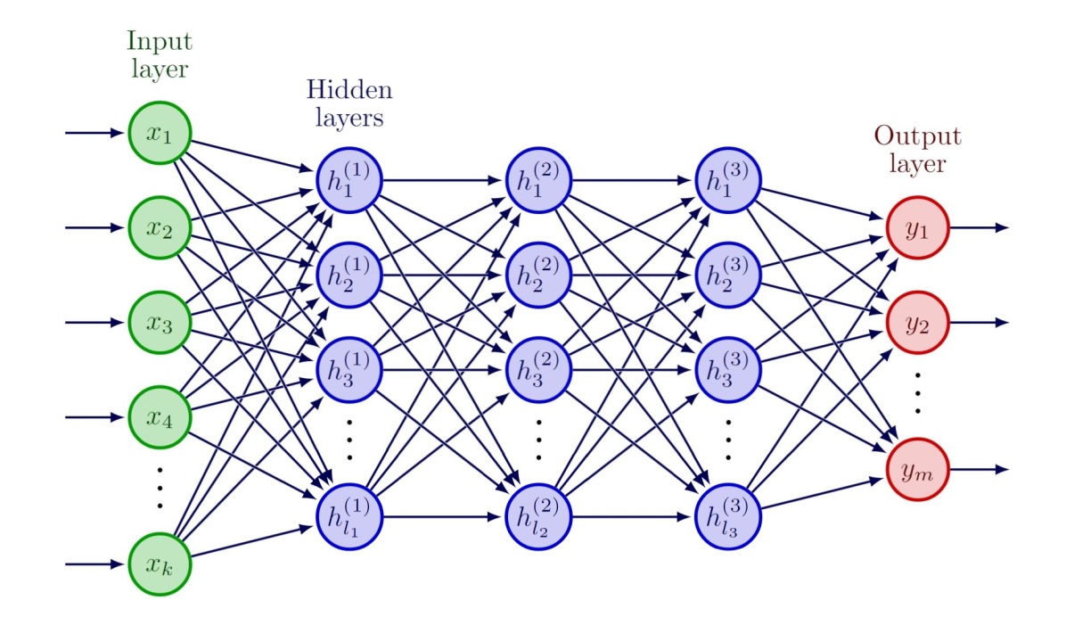
The model employed is a feed forward neural network with 3 hidden dense layers (Figure 1). Each hidden layer is followed by a batch normalization layer Ioffe and Szegedy (2015) and a dropout layer Srivastava et al. (2014). The NN is implemented in Tensorflow Abadi et al. (2015). The input layer has dimension $k=60$. Each of the first two hidden layers is composed of $2048$ neurons, while the third hidden layer hosts $1024$ neurons. The last (output) layer has $m=36$ neurons. Each of the output neurons is associated with a particular detector-energy combination. The probability parameter for the drouputs is $0.02$. The optimizer used is Nadam Ruder (2016) with learning rate $\eta$ varying accordingly to Equation 1, $\beta_{1}=0.9$, $\beta_{2}=0.99$ and $\epsilon=10^{-7}$.

$$\eta=\begin{cases}0.01&\text{if epoch $<4$}\\ 0.0016&\text{if $4\geq$ epoch $<12$}\\ 0.0004&\text{if epoch $\geq 12$}\end{cases}$$ (1)

We run the fitting for 64 epochs with a batch size of 2048.

Figure 1: The architecture of a feed forward neural network. The input has dimension 60. The first two hidden layer have 2048 neurons, the third 1024. The output layer has dimension 36.

In a pre-processing step, the input training dataset is standardised and filtered. Data filtering takes place in two steps in which the following data subsets are removed:

• data collected while Fermi is transiting through the high radiation environment of the South Atlantic Anomaly (SAA).

• data acquired at times in which an event of the Fermi/GBM trigger catalog occurred.

This latter choice isn’t strictly necessary, yet it is useful to better understand the neural network performances over known events. The splitting procedure divides the dataset in 75% train, 25% test; 30% of the training set is further kept as validation set. The resulting splitting is: 52% train, 23% validation and 25% test. The instances inside these sets are not sequential but rather taken randomly.

The purpose of our framework is to evaluate the effectiveness of our model on a known dataset, hence the choice of a loss function $L$ which is robust against outliers is critical. The Mean Square Error loss function (MSE) is:

$$\text{MSE}(x,y)=\frac{1}{n}\sum_{i=1}^{n}\left(y_{i}-x_{i}\right)^{2}.$$ (2)

MSE is very sensitive to the discrepancy between the prediction and the target value, thus it is a bad choice when outliers are present in the training dataset. We remark that the filtering of catalog events is not enough to guarantee the optimization of the background estimator when using MSE. Indeed, anomalous events, which are not present in the GBM catalog, may be over-fitted when minimizing MSE; these events are the actual targets of our search.

The Mean Absolute Error (MAE) loss function is less sensitive to residuals:

$$\text{MAE}(x,y)=\frac{1}{n}\sum_{i=1}^{n}\mid y_{i}-x_{i}\mid$$ (3)

In respect to MSE, MAE will result in better neural network performances when anomalous events are included in the training dataset. In the settings of multi-output regression, the overall loss $\mathcal{L}$ is define as the MAE average of the NN outputs:

$$\mathcal{L}=\frac{1}{m}\sum_{j=1}^{m}(\text{MAE}(F(X)_{j},Y_{j}))$$ (4)

2.2 Trigger algorithm

An efficient change-point and anomaly detection algorithm called FOCuS-Poisson (Functional Online CUSUM) Ward et al. (2022) is employed to find anomalous transients in Fermi CSPEC data relative to the NN estimates of the background.
The FOCuS-Poisson algorithm is executed sequentially over the time series of the observed count data and the background estimates, separately for each combination of detectors and energy range. For a given detector-energy range combination with label $i$ and a given time step $t$, FOCuS-Poisson outputs an estimate of the maximum significance in the observed count excess relative to the background, $m_{t}^{(i)}$. This value is computed over an optimal time interval ending at $t$ and starting at a past time-step $t-d$. Crucially, the interval length $d$ is not predetermined but rather assessed and optimized by the algorithm itself, conditionally on the observations. The significance values $m_{t}^{(i)}$ are recorded, in units of standard deviations, in a table with dimensions $M\times N$, where $M$ equals the length of the input time series and $N$ equals the number of detector-energy range combination. From these table, candidate transients are extrapolated in two steps. The first step is to identify vertical table slices (rows segments) where a trigger condition is verified. The second step is to cluster together segments whose start and end times are closer than a pre-defined value (nominally $600$ s).
The user controls the search’s output through three parameters. For the trigger condition to be verified it is required that the significance values exceed a threshold parameter $T$ over a minimum number detectors and energy ranges. Additionally, the user can limit the choice of the best interval to those whose length does not exceed a value $d_{\text{max}}$ or whose average intensity, given as a multiplicative factor of the observed counts in relation to the integral of background values, is greater than a minimum $\mu_{\text{min}}$.

3 Data

The Fermi/GBM daily CSPEC data products were used for both the testing and the training of the neural network and for searching astrophysical transient events with FOCuS-Poisson. These data are photon counts with duration $4.096$ s, binned over $128$ logarithmically spaced energy channels spanning from $\approx 8$ keV to $\approx 900$ keV Meegan et al. (2009). The time resolution provided by CSPEC data is high enough to investigate long and ultra-long GRBs, yet it is too low to reliably identify short GRBs and other transients with characteristic duration shorter than a few seconds. This is unfortunate, yet justified for our use-case. Indeed, the variability of background over time intervals of duration comparable to the duration of short GRBs is negligible, hence our method provides little benefits relative to simpler approaches such as moving average or exponential smoothing. On the other hand, an accurate description of the background become essential when searching for long, faint events, in particular events whose duration is comparable to that of the Fermi orbit. We consider data from all of the Fermi/GBM’s twelve NaI detectors. Each detector is identified according to the standard GBM nomenclature (ten detectors labelled with integers ranging from $0$ to $9$, two detectors are identified by the letters $a$ and $b)$. In our analysis we disregard the Fermi/GBM bismuth-germanate detectors. These instruments are in fact sensible to energies much greater than the energies typically involved with GRBs prompt emission and are mainly used for the detection and observation of phenomena different from GRBs, such as Terrestrial Gamma-Ray Flashes (TGF) Von Kienlin et al. (2020). To build the target variables $Y$, the input CSPEC data from each detector are binned anew, this time over three coarser energy ranges (28-50 keV, 50-300 keV and 300-500 keV, see Table 1). The resulting dataset is arranged in a table with $36$ columns, one for each of the $36$ detector-energy combinations.

Range	Energy range (keV)
r0	28-50
r1	50-300
r2	300-500

Table 1: Energy ranges table.

Beside the CSPEC data product, the neural network is trained using information on the satellite geographical location and the detectors pointing direction, as well as a number of auxiliary features such as the Earth occultation status and the visibility of the Sun for each detector at a given time. These informations are gathered from the Fermi/GBM POSHIST data products. A detail of the orbital and detectors features used in the training of the NN is given in Table 2 and Table 3. To access both the CSPEC and POSHIST data products we use the Fermi Data Tools package, a python software API to the HEASARC Fermi archival database. The resulting input datasets $X$ include a total of 60 different features, sampled with a step length of $4.096$ s.

Feature label	Description
$pos\_x$, $pos\_y$, $pos\_z$	position of Fermi in Earth inertial coordinates
$a$, $b$, $c$, $d$	Fermi attitude quaternions
$lat$	Fermi geographical latitude
$lon$	Fermi geographical longitude
$alt$	Fermi orbital altitude
$vx$, $vy$, $vz$	velocity of Fermi in Earth inertial coordinates
$w1$, $w2$, $w3$	Fermi angular velocity
$sun\_vis$	Sun’s visibility boolean flag.
$sun\_ra$	Sun’s right ascension
$sun\_dec$	Sun’s declination
$earth\_r$	Earth’s apparent radius
$earth\_ra$	Earth center right ascension
$earth\_dec$	Earth center declination
$saa$	SAA transit boolean flag
$l$	approximate McIlwain L value

Table 2: A table of the 24 orbital features used to form the NN’s input table. The features are obtained from the POSHIST files and processed by the library Fermi GBM Data Tools.

Features	Description
$ni\_ra$	$i$-labelled detector pointing right ascension
$ni\_dec$	$i$-labelled detector pointing declination
$ni\_vis$	$i$-labelled detector Earth occulation boolean flag

Table 3: A table of the 36 detector features used to form the NN’s input table. The features are obtained from the POSHIST files and processed by the library Fermi GBM Data Tools.

4 Results

In this section we present the results of the background estimator and the trigger algorithm application. The open source code implementation is available on github.com/rcrupi/DeepGRB.

4.1 Background estimator performance

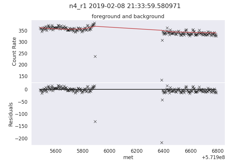
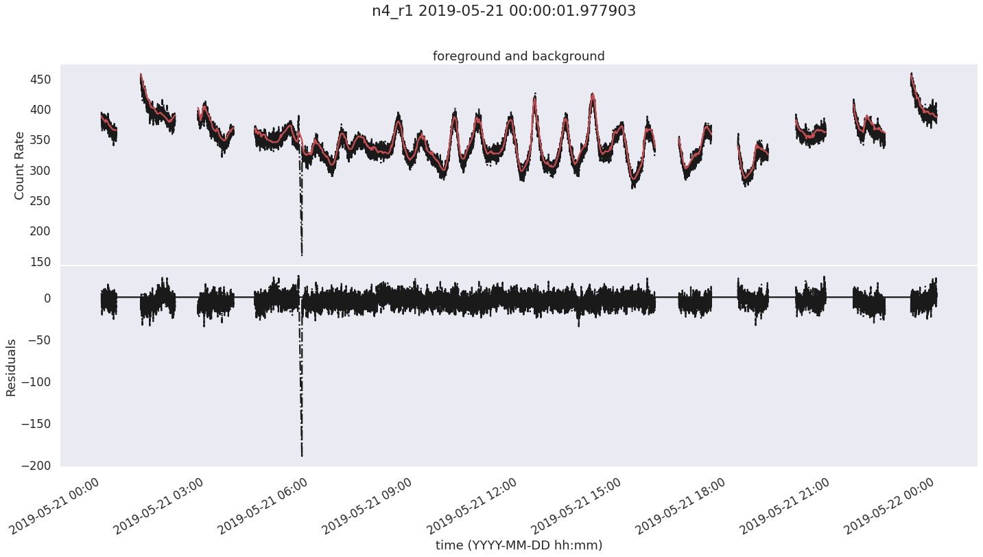
To show the effectiveness of this approach, a NN is trained over 7 months of data from January to July 2019. An excerpt of the resulting background estimation is presented in Figure 3 for one detector-range combination. The MAE values are reported in Table 4. The energy range bins are the same as those used in Section 3 and are defined in Table 1.

det range	MAE train	MAE test
r0	4.942 $\pm$ 0.331	4.953 $\pm$ 0.328
r1	6.088 $\pm$ 0.167	6.098 $\pm$ 0.163
r2	1.790 $\pm$ 0.044	1.792 $\pm$ 0.045
average	4.273	4.281

Table 4: The NN MAE loss function (within one standard deviation) per energy range, over the training and the testing datasets, averaged over the 12 Fermi’s GBM NaI detectors.

In Appendix A, the NN background prediction over a dataset comprising GRB091024 are compared to the results of an established physical Fermi/GBM background model Biltzinger et al. (2020).

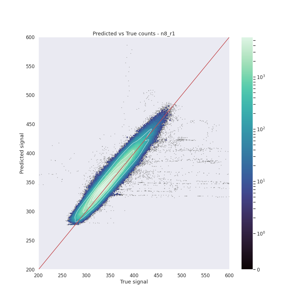
In Figure 4 we plot the NN predictions against the corresponding observed value, in particular we filtered out the data points 150 s before and after the SAA. Figure 4 depicts a light-curve with background counts greater than those observed, we discuss this phenomenon later in this Section 5.

Figure 2: Fermi/GBM NaI-4 detector photon count rates (crosses) in the energy range $50$ - $300$ keV versus the respective prediction from the Neural Network (red solid lines). The lower panel shows the residuals between the two quantities, with a black solid line denoting the reference of null residual. Data span $1400$ s and one SAA crossing. Three data events appear to be anomalously low, possibly due to lengthy instrument switch-on and switch-off procedures.

The events of interest for this research should be found when the observed count rates exceed the NN prediction, that are the points below the bisector (see Figure 4) for detectors-range combination. Transient, bright events such as GRBs may result in a temporary increase of the observed count rates and, taking place at random times and directions, are not predictable from features intrinsic to the Fermi spacecraft motion and attitude, which are the actual inputs of the NN.

Figure 3: The background estimation for the n4 detector, in the energy range 1, on one day orbit. The Fermi/GBM count rate observations are represented over time as a black line, whereas the neural network estimation is plotted as a red solid line. The lower panel shows the residuals between the two quantities, with a black solid line denoting the reference of null residual.

Figure 4: Fermi/GBM photons counts from NaI-8 detector in the energy range $50$ - $300$ keV versus the respective prediction from the NN over the same combination of detector and energy range. Data spans from 1 January 2019 to 1 July 2019.

The three time periods chosen for the application of the trigger algorithm spans 1 November 2010 to 19 February 2011, 1 January 2014 to 28 February 2014, 1 March 2019 to 9 July 2019. For the sake of brevity, we will refer to these epochs as the ‘2010’, the ‘2014’ and the ‘2019’ periods. These periods are chosen to test the framework under a variety of conditions, including solar activity intensities and potential detector degradation.

A separate NN is trained and tested for each of these periods to account for variations in background count rates over long time scales (years), which may be caused by factors such as the two previously mentioned. We report the performance metrics in Table 5.

NN performance metrics on test set
Period	Energy range	MAE	MeAE
2010	r0	7.730 $\pm$ 4.842	3.963 $\pm$ 0.232
2010	r1	6.469 $\pm$ 1.517	4.777 $\pm$ 0.100
2010	r2	1.864 $\pm$ 0.033	1.563 $\pm$ 0.028
2014	r0	19.79 $\pm$ 18.92	4.545 $\pm$ 0.409
2014	r1	13.29 $\pm$ 11.10	5.604 $\pm$ 0.196
2014	r2	1.949 $\pm$ 0.099	1.598 $\pm$ 0.082
2019	r0	4.831 $\pm$ 0.300	3.938 $\pm$ 0.245
2019	r1	5.640 $\pm$ 0.082	4.716 $\pm$ 0.070
2019	r2	1.804 $\pm$ 0.038	1.510 $\pm$ 0.032

Table 5: Mean Absolute Error (MAE) and Median Absolute Error (MeAE), on the test datasets, for each energy range and averaged for detectors within one standard deviation.

Additional details on the neural network’s performance during times of both high and low solar activity are provided in Appendix C.

4.2 Transients detection

With reference to the technique described in Section 2.2, the following detection parameters were used to obtain the results discussed in this section. The trigger condition was defined to resolve whenever at least one detector observed enough counts for the significance level to exceed a threshold $T=3\sigma$ over the range of energy spanning $50$ keV and $300$ keV.

To measure the consistency of the entire event it is computed the Standard Score $z$:

$$z=\frac{x-\mu}{\sigma}$$ (5)

where $\mu$ is the mean and $\sigma$ the standard deviation of the distribution $\mathcal{X}$. Since we are dealing with count rates that follows the Poisson distribution, with sufficiently high count rates we can consider $\mu\approx\sigma^{2}$. Then the Standard Score can be approximated to:

$$S=\frac{N-B}{\sqrt{B}}$$ (6)

where $N$ is the observed count rates integrated over an interval spanning the event’s start time and end time and over each triggered detectors. Analogously for $B$ but the total count rates comes from the background estimated by the NN. Standard Score is determined independently for each energy range $S_{r0}$, $S_{r1}$ and $S_{r2}$. The overall consistency for the event is defined as:

$$C=max(S_{r0},\;S_{r1},\;S_{r2}).$$ (7)

The FOCuS-Poisson algorithm was executed with the parameters $d_{\text{max}}$ and $\mu_{\text{min}}$ set to the values $120.4$ s and $1.2$ s, respectively. The choice of these parameters was driven by a trade-off between the need to find most astrophysical transients in our dataset both known and potentially unknown and the need to minimize the rate of false detection.
The transient search was performed over three distinct time periods, as defined in the previous section. In the period spanning March 2019 and July 2019 a total of 100 events were identified. Of these, 75 events match the trigger time of events already in the Fermi/GBM Trigger Catalog Von Kienlin et al. (2020), one event is due to artifacts in the dataset, while the nature of the remaining 24 events is uncertain. These results, along other from the remaining test periods, have been summarized in Table 6. Over the same period, the Fermi/GBM Burst Catalog Von Kienlin et al. (2020) reports on 96 known GRBs. Of these bursts, 15 are missing a counterpart in our dataset due to the clipping of data $150$ s before and after a SAA transit. Of the remaining 76 bursts, 68 have $T_{90}$ duration larger than the bin-length resolution of our dataset ($4.096$ s). We were able to correctly identify $60$ of these bursts ($88\%$). Finally, we detected 5 out of 13 ($34\%$) GRBs with $T_{90}$ duration inferior to the the bin-lenght resolution of our dataset. These results are summarized in Figure 5 and Table 7, the latter also reporting on results from other periods.

Transient detection statistics
Period	Total events	Known	Consistency median known	Unknown	Consistency median unknown	False Detections
2010	81	58	$>10$	15	8.83	8
2014	195	81	$>10$	71	$>10$	43
2019	100	75	$>10$	24	8.71	1

Table 6: Total number of transients identified, number of transients with counterparts in the Fermi/GBM Trigger Catalog and its median consistency; number of transients of uncertain origin with no counterparts in the Fermi/GBM Trigger Catalog and its median consistency; false detection. Each table row corresponds to a different time period.

Known GRBs detection statistic
Period	Total GRBs	Missing (no data)	$T_{90}>4.096$ s	$T_{90}<4.096$ s
2010	77	11	39/52 (75 %)	2/14 (14 %)
2014	36	8	17/18 (94 %)	4/10 (40 %)
2019	96	15	60/68 (88 %)	5/13 (34 %)

Table 7: Total number of Fermi/GRBs in the Fermi/GBM Burst Catalog, number of events with missing (no data) counterparts in our dataset due to SAA data clipping (see Section 4.2), fraction of detected bursts with duration greater than the bin-length time resolution of the tested dataset, fraction of detected bursts with duration smaller than the bin-length time resolution of the tested dataset. Each table row corresponds to a different time period.

Figure 5: GRB detection performances. Each dot represents a gamma-ray burst of the Fermi/GBM Burst Catalog discovered between March 1st and July 1st 2019 over the space spanned by the GRB’s duration $T_{90}$ and flux, the latter computed as the ratio between the catalog’s GRB fluence in band 10-1000 keV and $T_{90}$). Events in the shaded grey region have $T_{90}$ duration smaller than the bin-length time resolution of the dataset tested with the present framework ($4.096$ s, CSPEC data). Colors are used to identify the detection status within our search. In red the events unidentified with our method. Missing events (no data) are due to clipping of data 150 s before and after a SAA transit or portion of data that could not be preprocessed.

5 Discussion

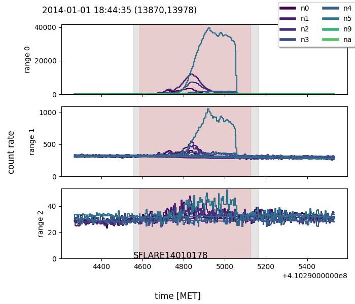
According to Tables 4 the test set and train set MAE values are similar up to $1\%$ indicating no over-fitting and strong generalization across energy range and detector. Table 5 shows that the neural network trained on data from the 2014 period has the highest (worst) MAE, which can be attributed to the presence of strong solar activity. This is understandable since, during an activity maximum, the background particle count rate is more unpredictable due to the influence of the Sun on the local radiation environment (see Figure 6(b)). Nonetheless, MeAE shows similar performance with the other two periods, thanks to its robustness against outliers. On the other hand, the 2019 period has the lowest MAE most likely due to low solar activity and low background variability. For more details on predictive robustness against high solar activity see Appendix C.

In Figure 4, most of the data points are distributed along the plot bisector $y=x$, indicating that most often the neural network estimate is in agreement with the actual observations. Above the bisector, more counts are expected than they are actually observed. From spot analysis of these datapoints it is apparent that overestimates in NN prediction often happen when Fermi enters or leaves the SAA, see for example Figure 2. A possible explanation of this behaviour can be rooted in the Fermi/GBM experimental apparatus. Fermi/GBM is composed of multiple photomultipliers. These instruments require high voltages to operate. A “ramp-up" of a photomultiplier to operational voltage takes place over a time span of several seconds. During this time, the photomultiplier amplification factor (the gain) is hindered resulting in lower than nominal count rates. The same effect takes place when “ramping-down" before turning a photomultiplier off. In the lower part of the bisector the observed counts rate exceed the counts estimated. The trigger algorithm’s goal is to determine whether this exceeding amount is part of an event or simply a random fluctuation.

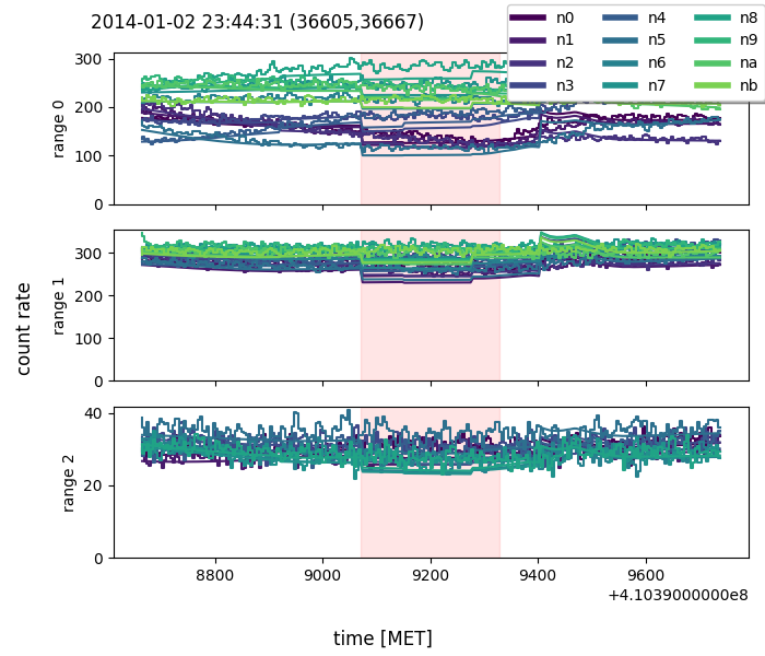
In periods of high solar activity, Fermi/GBM data include a large number of soft transient events of solar origin; thus, the soft ($25$ - $50$ keV) trigger conditions have been disabled on multiple occasions (e.g. see Table 4 in Bhat et al. (2016) for 2014). Likewise, we required that at least one detector must be over threshold in the energy band spanning $50$ and $300$ keV in order for the trigger condition to be satisfied. Still, Table 6 shows a higher number of total events for the 2014 period. The majority of these events are most likely associated to solar flares; indeed, 50 of the 81 events in the GBM trigger catalog for this period are solar flares, and the majority of the events we find with no counterpart in the Fermi/GBM trigger catalog are triggered over Sun facing detectors (n0, n1, n2, n3, n4, n5). False detections may be caused by artifacts in the background estimation. These are generally easy to identify; most of the time these artifacts take the form of sudden steps in the background estimate, simultaneously over all detector/range combination. One of these events is represented in Figure 6(a). This behaviour is less frequently present in the other two periods analyzed, indicating that noisy background impacts on performance (see MAE) and therefore more false positive are detected.

(a)

(b)

Figure 6: Photon counts from each triggered detector are plotted with step lines, across three energy bands spanning $28-50$ keV, $50-300$ keV and $300-500$ keV (Table 1), with a resolution of $4.096$ s. The neural network’s prediction of background count rates is represented by solid lines. Different detectors are identified using different colors. A red shaded area limits FOCuS-Poisson’s best guess of the transient duration. Times are expressed in units of seconds according to Fermi’s standard mission elapsed time (MET). (a) Example of False Detection in which all the detector are triggered over an imprecision of the Neural Network estimation. (b) Example of a solar flare in the Fermi/GBM catalog detected by our approach. The event start and end MET time, as reported in the Fermi/GBM trigger catalog, is represented by a grey shaded area.

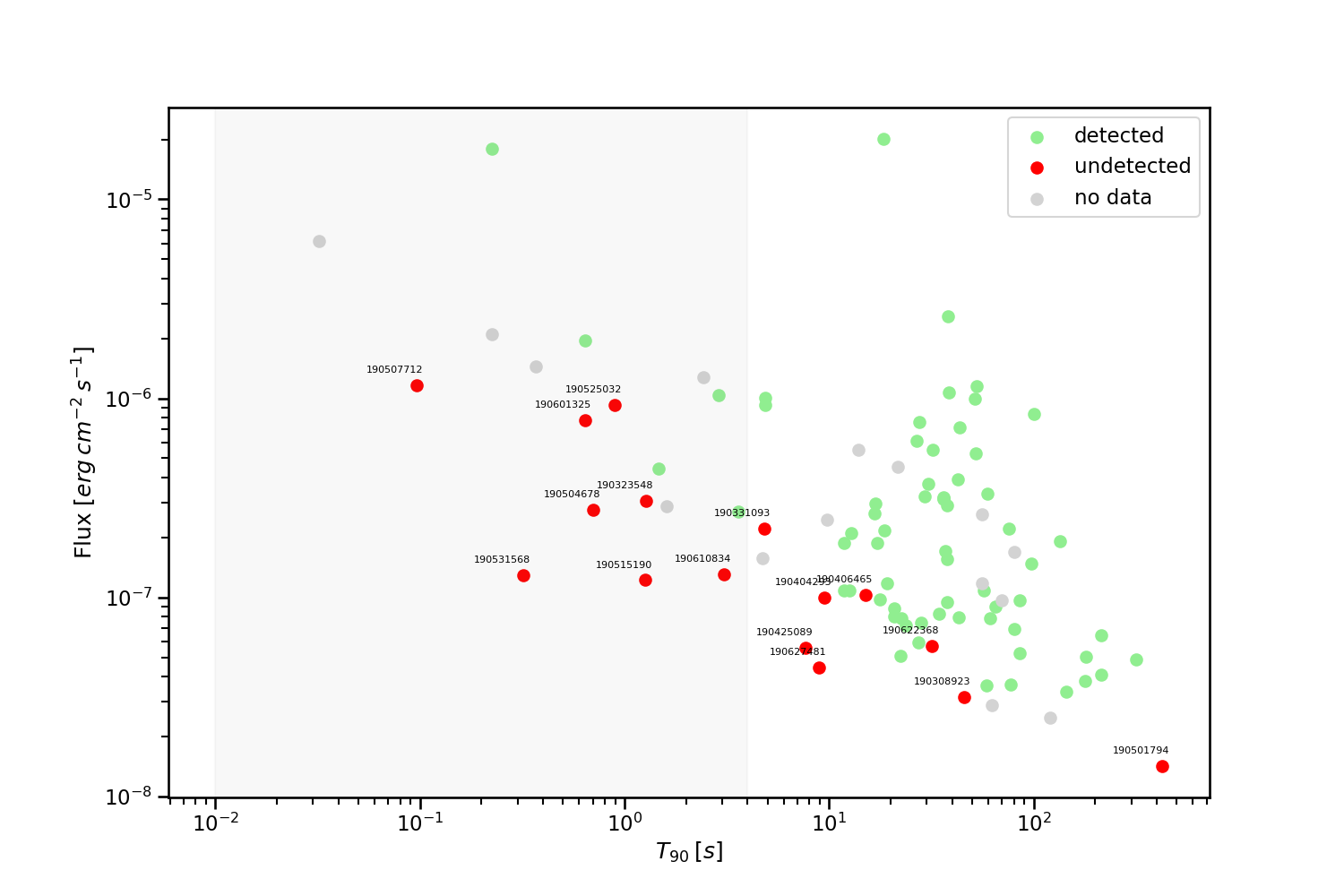
To further investigate the detected and undetected GRBs, we plot the flux (total fluence divided by T90) vs T90 for our triggered events in Figure 5. The red points are events reported in the Fermi/GBM catalog but undetected by our method. The Fermi/GBM events with a duration less than our time binning (4.096s) are often undetected in our analysis because of the too coarse binning. We also miss a few longer events with low count rates. Reducing the time binning by using data with higher time resolution, such as CTIME or TTE, could be beneficial to capture shorter and fainter events. Despite the unfavorable adopted time binning of 4.096s, we recovered $\geq 75\%$ of the GRBs with $T_{90}$ greater than 4.096s, see Table 7.

We also detect many events not present in the Fermi/GBM catalog, and we use the methodology outlined in Kommers (1999) to characterize these transients. More specifically, we classify events as:

• Solar flare (SF) when the majority of the counts are in the low-energy range and the Sun is in the field of view of the triggered detectors.

• Terrestrial Gamma-ray Flash (TGF) when most of the counts are in the high-energy range and the event’s source reaches the detector from the Earth’s horizon.

• Gamma-ray burst (GRB) when most of the counts are in the $50-300$keV energy range, and the source direction is not occulted by the Earth and is distant from both the Sun and the galactic plane.

• Galactic X-ray flash (GF) when the source direction is compatible with that of the galactic plane.

• Uncertain (UNC) in all other cases.

To determine the source direction, we employ a simple method based on the evaluation of the pointing and the relative photon count rate of the detectors. Further details can be found in Appendix B.

Two classes of transient events are discussed further in this section: events already classified as GRBs in the Fermi/GBM trigger catalog; events not present in the Fermi/GBM catalog but classified by us as candidate GRBs. We report In Table 8 six more events that have no catalog counterpart, suggesting one or more of the previously mentioned categories. All these events are a cherry pick selection of the unknown events in Table LABEL:tab:catalog_unk.

GRB 190320A

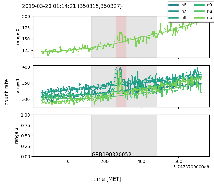
At 01:14:16 UTC on March 20, 2019, the long GRB 190320052 triggered the Fermi/GBM on board trigger algorithm across detectors n6 and n9. The estimated $T_{90}$ duration is $43$ s, with the highest emission component in the $50$-$300$ keV band. In our analysis, the detectors n6, n7, n8, n9 and na all exceeded a $3.0$ $\sigma$ significance threshold during the period event (Figure 7) with a resulting consistency greater than $10$ on energy range r1 and $5.74$ on r2. The background estimate is comparable to a second order polynomial fitting in the soft energy range and first order polynomial fitting in the $50$-$300$ keV energy range.

Figure 7: The Fermi/GBM catalog GRB190320, as detected by our method. Photon counts from each triggered detector are plotted with step lines, across three energy bands spanning $28-50$ keV, $50-300$ keV and $300-500$ keV (Table 1), with a resolution of $4.096$ s. The neural network’s prediction of background count rates is represented by solid lines. Different detectors are identified using different colors. The GRB start and end MET time, as reported in the Fermi/GBM burst catalog, is represented by a grey shaded area. A red shaded area limits FOCuS-Poisson’s best guess of the transient duration. Times are expressed in units of seconds according Fermi’s standard mission elapsed time (MET).

Event 190420939

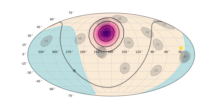
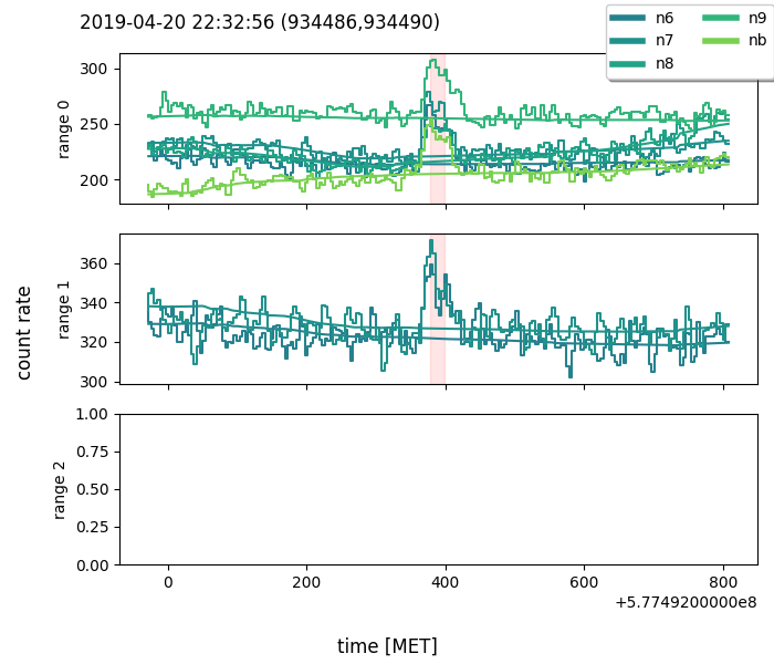
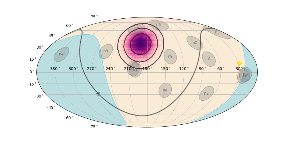
Figure 8 shows an event not present in the GBM trigger catalog, similar to GRB190320052 but with higher low-energy count rate. The event has been triggered by detectors n6, n7, n8, na and nb in the low energy band with a consistency greater than $10$. Two detectors provided a trigger in the $50$-$300$ keV energy band, with a consistency of $8.4$.

Figure 8: The 190420939 transient event with no direct counter part in the Fermi/GBM trigger catalog. The event was classified as a candidate gamma-ray burst, according to the discussion presented in Section 5. For the corresponding localization see Figure 9. Photon counts from each triggered detector are plotted with step lines, across three energy bands spanning $28-50$ keV, $50-300$ keV and $300-500$ keV (Table 1), with a resolution of $4.096$ s. The neural network’s prediction of background count rates is represented by solid lines. Different detectors are identified using different colors. A red shaded area limits FOCuS-Poisson’s best guess of the transient duration. Times are expressed in units of seconds according Fermi’s standard mission elapsed time (MET).

We can see from the localization estimate in Figure 9 that the event is far from the galactic plane, the Sun, and the Earth’s horizon. With all of this information, this event could be a long soft GRB. The localization algorithm used is described in detail in Section B.

Figure 9: Estimate of the candidate event’s source localization over the celestial sphere at 2019-04-20 22:32:56 UTC.

Interesting events

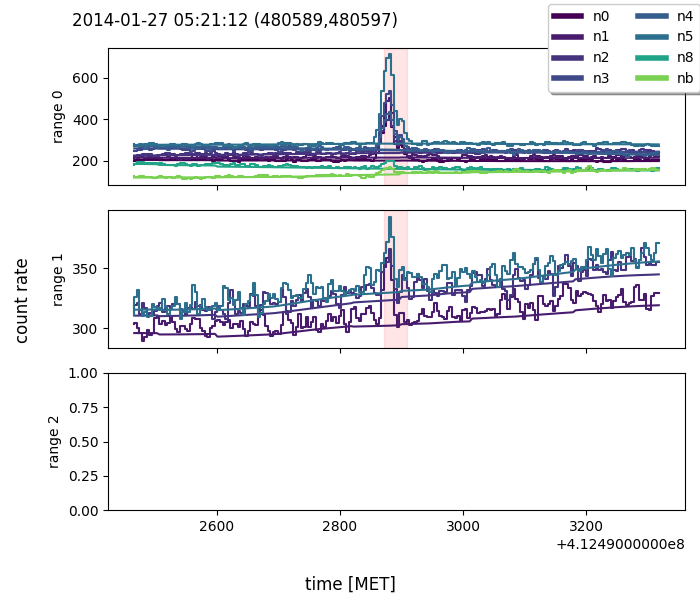
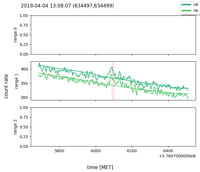
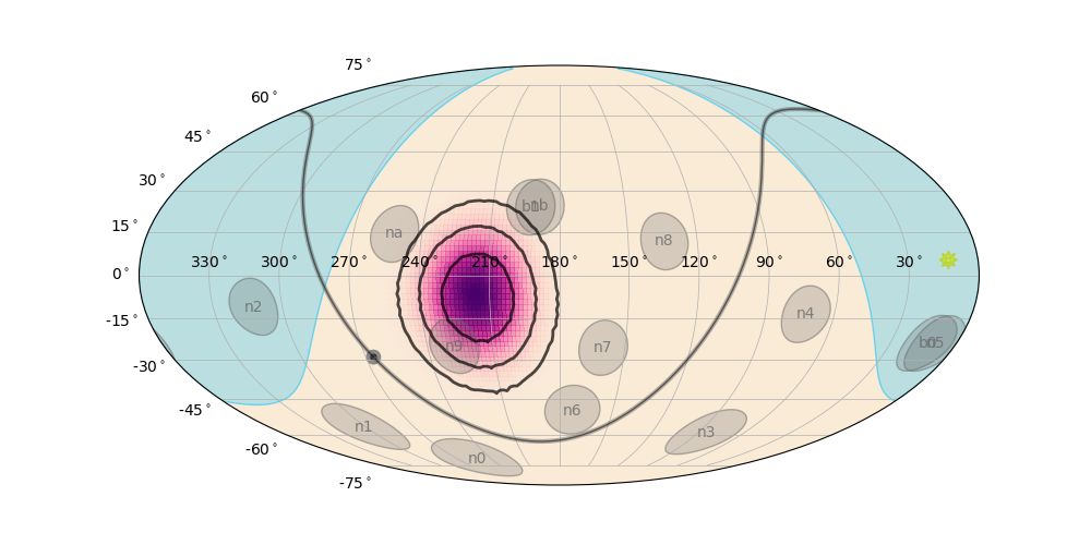
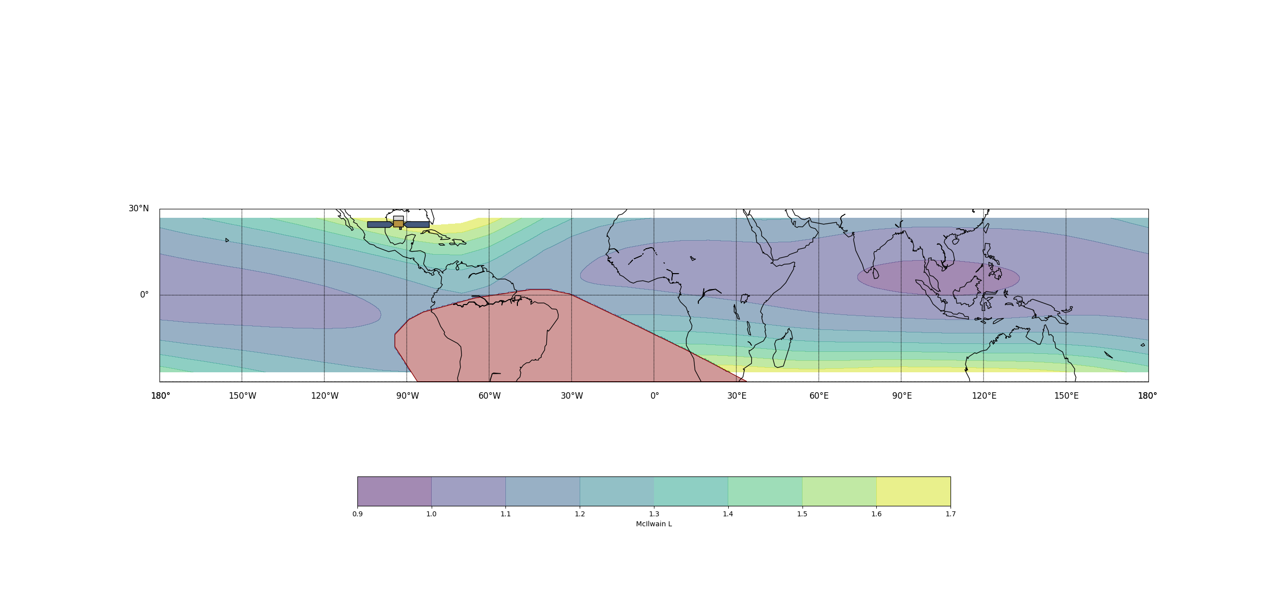
We list in Table 8 a selection of interesting events, including the one already discussed, which are not present in the GBM catalog and which deserve further analysis. Appendix D present plots associated to these events. Events 1 and 2 are classified as Solar Flares because their location is close to the Sun and the majority of the detectors triggered are in the energy range r0. Because event 3 is far from the Sun yet close to the galactic plane and the Earth’s horizon, it might be a Galactic X-ray flash or a Terrestrial Gamma-ray Flash. Event 4 and 6 are categorized as GRBs for the same reasons as event 5, however because they are near the galactic plane, event 6 might be a Galactic X-ray burst. Finally, in event 7, nine detectors with roughly equal intensities are triggered, suggesting that this event is likely due to Local Particles. This is further validated by the satellite’s position at high geomagnetic latitude (Figure 22), which is highly correlated with the localization of charged particle events Von Kienlin et al. (2020); as a result, the event is classified as uncertain.

It’s worth noting that GRB 190404B GCN Circular notice discovered by Monitor of all-sky X-ray image (MAXI) satellite has location $(\text{RA}=221^{\circ},\text{Dec}=-22^{\circ})$, which is similar to event 4, and trigger time 2019/04/04 13:14:34.00 UTC, which is six minutes after event 4.

The complete catalog of unknown and known events for the three time periods analyzed can be found in Appendix in Tables LABEL:tab:catalog_unk and LABEL:tab:catalog_kn, respectively. The events are reported with the trigger time, duration, the triggered detectors, the Standard Score for each energy range, and a significance classification. Unknown events were assigned tentative transient classes using the methodology described in this section.

ID	Trigger time	T (s)	Detectors triggered	RA (∘)	Dec (∘)	Transient class	C
1	2014-01-27 05:21:12	32.77	n0 n1 n2 n3 n4 n5 n8 nb	306	-22	SF	$>10$
2	2010-11-11 18:58:17	16.38	n2 n4 n5	230	-20	SF	$>10$
3	2014-01-12 13:59:58	102.40	n6 n7 n8 n9 na nb	105	10	GF/TGF	$>10$
4	2019-04-04 13:08:07	8.19	n9 na	220	-10	GRB	4.93
5	2019-04-20 22:32:56	16.38	n6 n7 n8 n9 nb	245	40	GRB	$>10$
6	2019-06-06 13:21:42	16.38	n7 n8 nb	250	25	GRB/GF	9.12
7	2011-02-15 15:59:02	118.79	n0 n1 n2 n5 n6 n7 n8 n9 nb	208	62	UNC	$>10$

Table 8: List of interesting events. We report the ID, the start time in MET and UTC, the end time in MET, the detectors triggered during the event, the localisation expressed in right ascension and declination, the proposed transient class and the consistency of the event

.

6 Conclusion

A novel method for high-energy, transient event detection is presented, integrating the precise estimation of a NN with an efficient trigger algorithm. The method has been designed to be applied to HERMES Pathfinder data, but it can be extended to analyze data from other space-based, high-energy missions and we have presented here an application using Fermi/GBM data. The first step is to estimate the background count rate with a NN using satellite data that may be used to build a physical background model. The accuracy of the background estimate is measured using Mean Absolute Error and Median Absolute Error. An experiment is carried out to assess the robustness of the background estimator during the periods of solar maxima (2014) and solar minima (2020), demonstrating that the background estimation is stable enough to have comparable performance in both periods. Because HERMES Pathfinder will be deployed near the next solar maximum, a scenario of expected count rates is provided in Appendix. The background is then used by FOCuS-Poisson, an evolution of the CUSUM algorithm, to efficiently detect the transient events. This method is tested using three periods of Fermi/GBM data binned in time for 4s. We provide statistics on known and unknown transients in the GBM catalog. We show that with our method we are able to recover known events longer than 4s, and to selected events not included in the Fermi/GBM catalog. Seven of the unknown events are discussed in details. Future work will aim to improve neural network prediction, such as employing a Recurrent Neural Network to provide a smoother signal or reducing time binning to detect shorter events. Also, provide explainability methods to allow the user to explain a specific prediction or debug the NN.

Appendix A Background estimate for GRB 091024

To demonstrate the potential of the background estimator in the presence of a long event, a background estimation is performed in a period containing the ultra-long GRB 091024 Gruber et al. [2011], for which a similar evaluation is provided in Biltzinger et al. [2020].

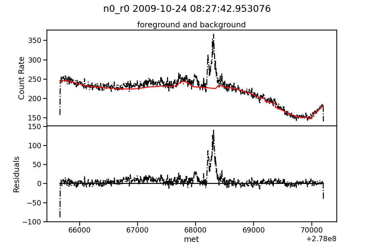
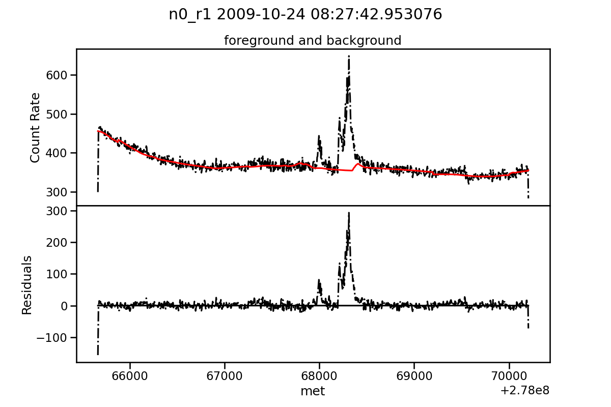
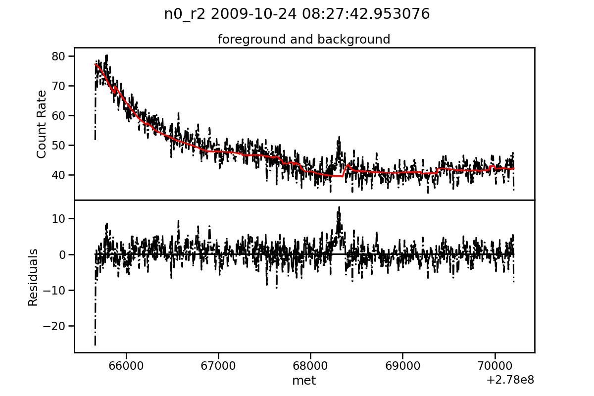
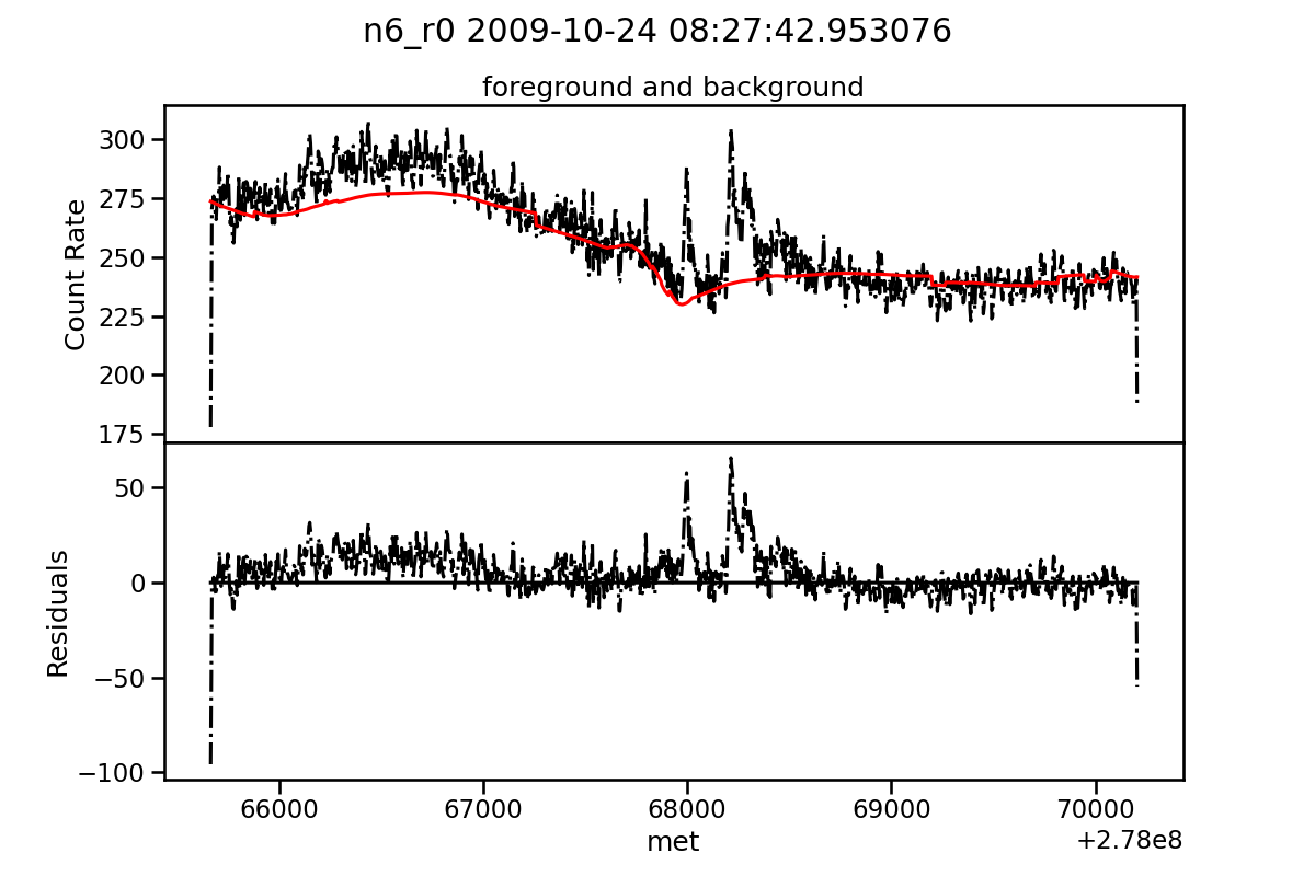
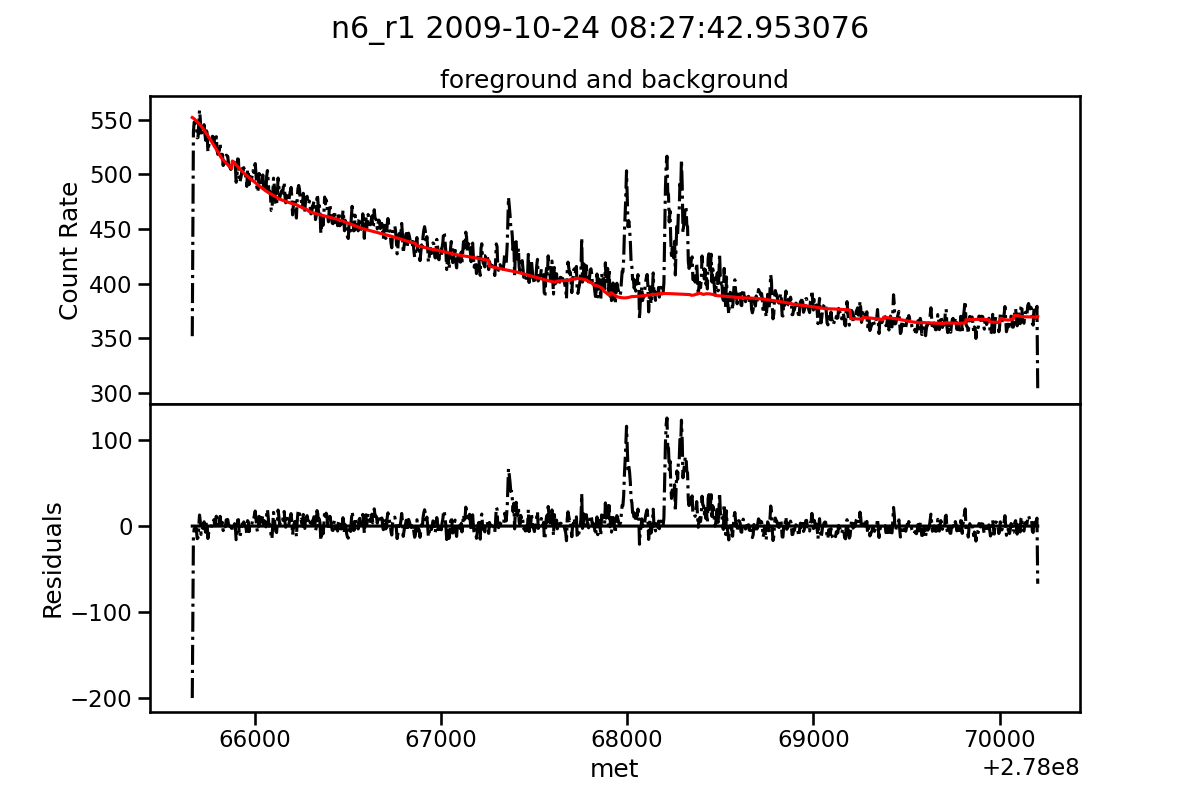
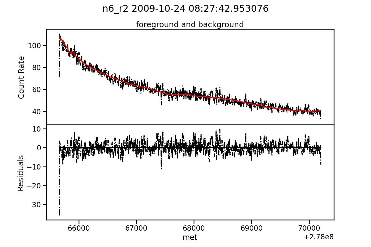
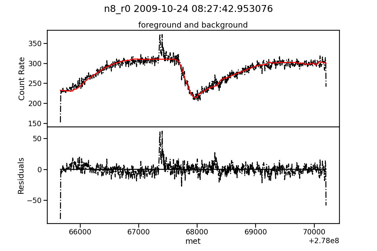
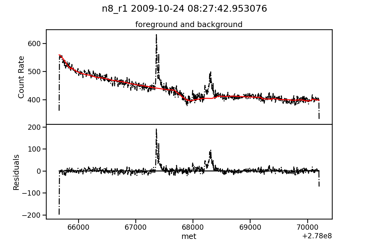
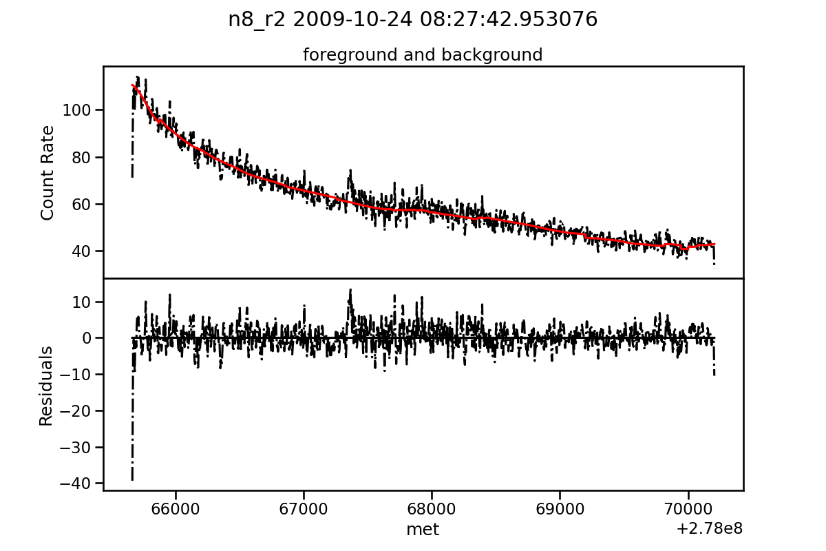
In Figure 10 are shown detectors n0, n6 and n8 in the three energy band specified in Table 1. The data and background estimation of a Neural Network trained and tested during a three-month period, from September 1 to November 30, 2009, are presented in black and red, respectively. The dataset consists of 1.63 million of samples and the hyperparameters are the same used in Section 2.1 except for the learning rate

$$\eta=\begin{cases}0.025&\text{if epoch $<4$}\\ 0.004&\text{if $4\geq$ epoch $<12$}\\ 0.001&\text{if epoch $\geq 12$}\end{cases}.$$

The event emerges clearly from the residuals of all the detectors in range r1 and r2, in detector n0 and range r2 it is still visible a peak probably belonging to the end of it. In detector n6 range r0, in the first part of the time series before the peaks of the event, the background estimation underestimates the foreground (data observed). This could be due to a too short period of training dataset, a non optimal parameter settings of the NN, a different event such as Local Particles or, more interestingly, the first part of the GRB, where photon counts were too low to be detected due to background variability.

Figure 10: Observed and background estimate count rates around the event GRB 091024. From left to right the plots refer respectively to range r0, r1, r2, from top to bottom the plots refer respectively to detectors n0, n6, n8. This figure can be compared with Figure 18 in Biltzinger et al. [2020].

Appendix B Localization

For the standard reference for the localization of events found by GBM, look Goldstein et al. [2020].
In this work the localization is done by a simple geometric reasoning, but in future we hope to use more sophisticated algorithm of localization. To optimise the function loss it is employed a particle swarm optimiser.

Consider two vectors in the equatorial coordinates $\psi_{d}=(ra_{d},dec_{d})$ and $\psi_{s}=(ra_{s},dec_{s})$, respectively the pointing of a detector and the localization of the event source. The incidence intensity is modeled as the cosine between the angle $cos(\psi_{d},\psi_{s})$ is:

$$cos(\psi_{d},\psi_{s}) =cos(\psi_{d,ra})cos(\psi_{d,dec})cos(\psi_{s,ra})cos(\psi_{s,dec})+$$

$$+sin(\psi_{d,ra})cos(\psi_{d,dec})sin(\psi_{s,ra})cos(\psi_{s,dec})+$$

$$+sin(\psi_{d,dec})sin(\psi_{s,dec})$$

If the angle of incidence is grater than $\pi/2$ than the incident intensity must be set to 0. Finally we have 8

$$\mathcal{I}(\psi_{d},\psi_{s})=max(cos(\psi_{d},\psi_{s}),0)$$ (8)

The loss to optimise in Equation 9, where $i$ is a particular detector in $D$ detectors (in our case 12). The energy range chosen is the one with the biggest residuals among detectors/energy ranges, then the count rates corresponding to the timestamp of the maximum value is given to the loss 9 and minimized.

$$\frac{\sum_{i=1}^{D}(counts_{s}(\mathcal{I}(\psi_{i},\psi_{s}))-counts_{i})^{2}}{D}$$ (9)

where $\psi_{s}$ and $counts_{s}$ are the unknown variables.

Appendix C Solar minima and maxima

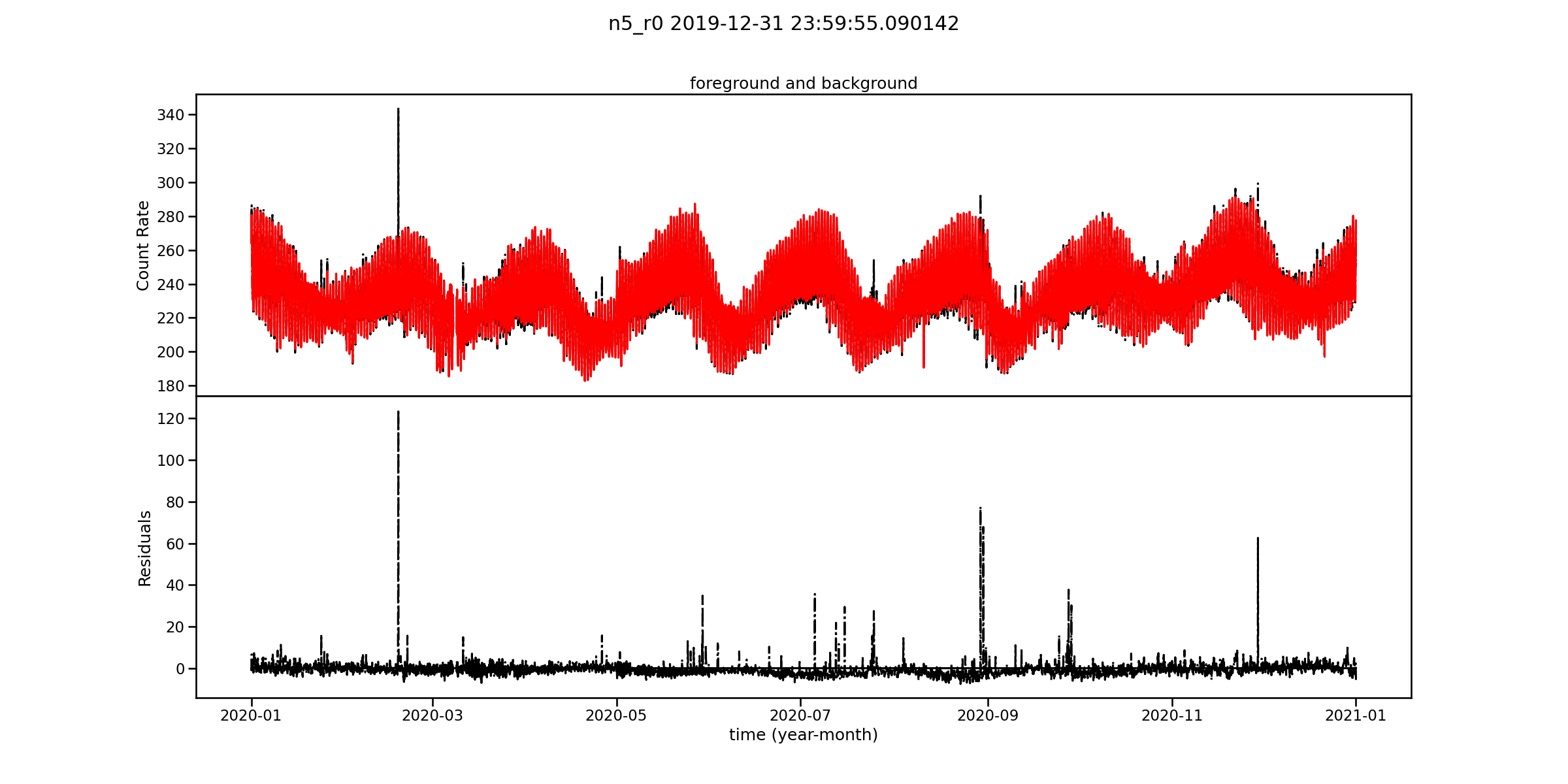
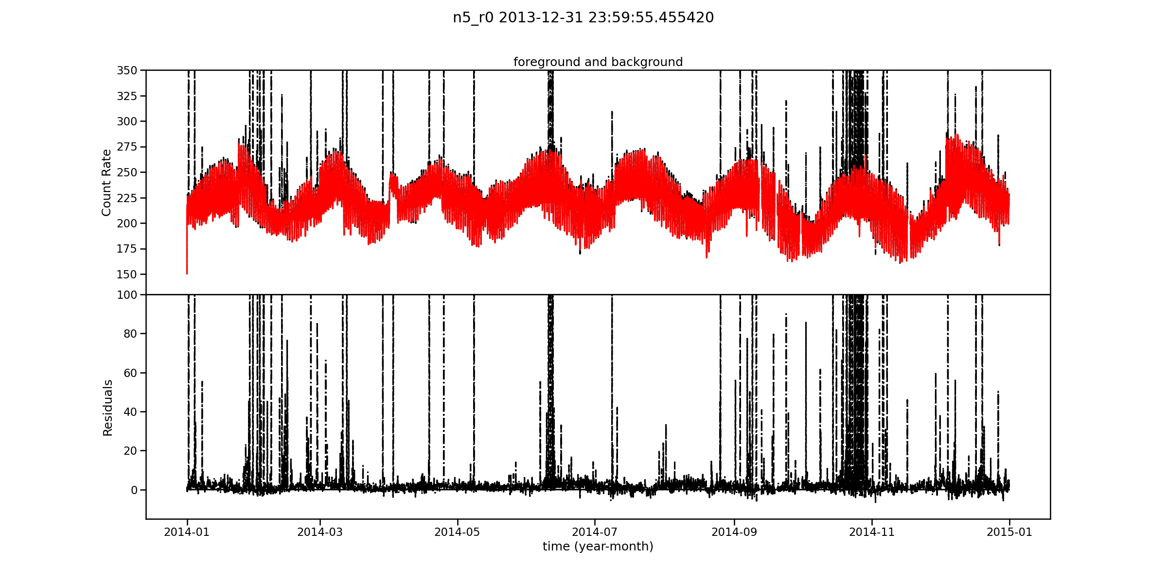
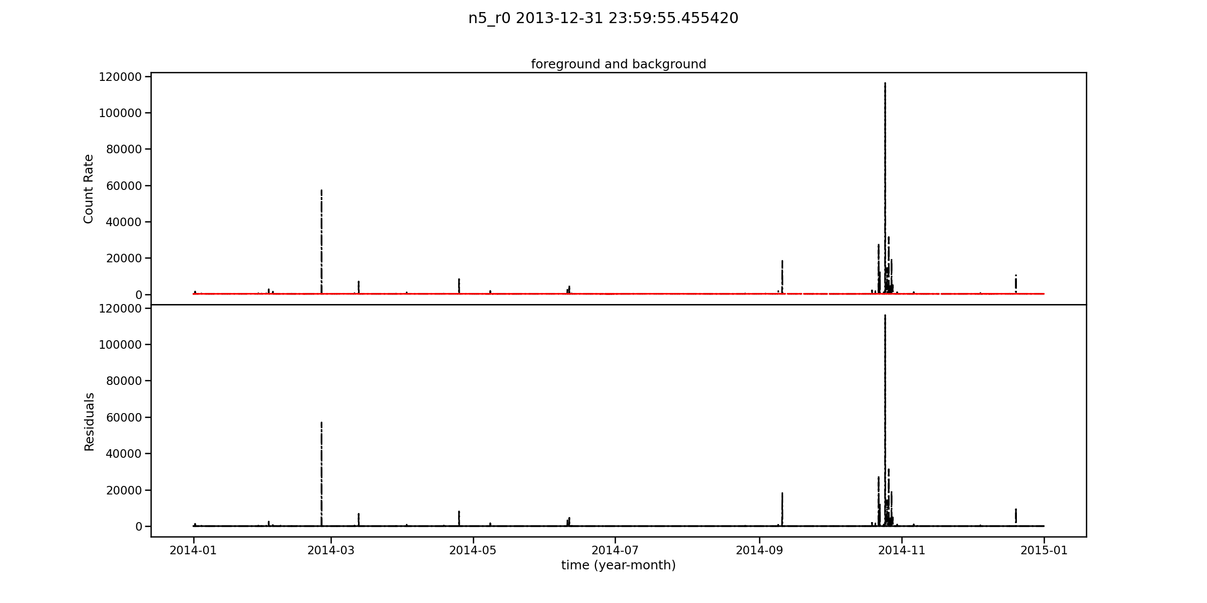
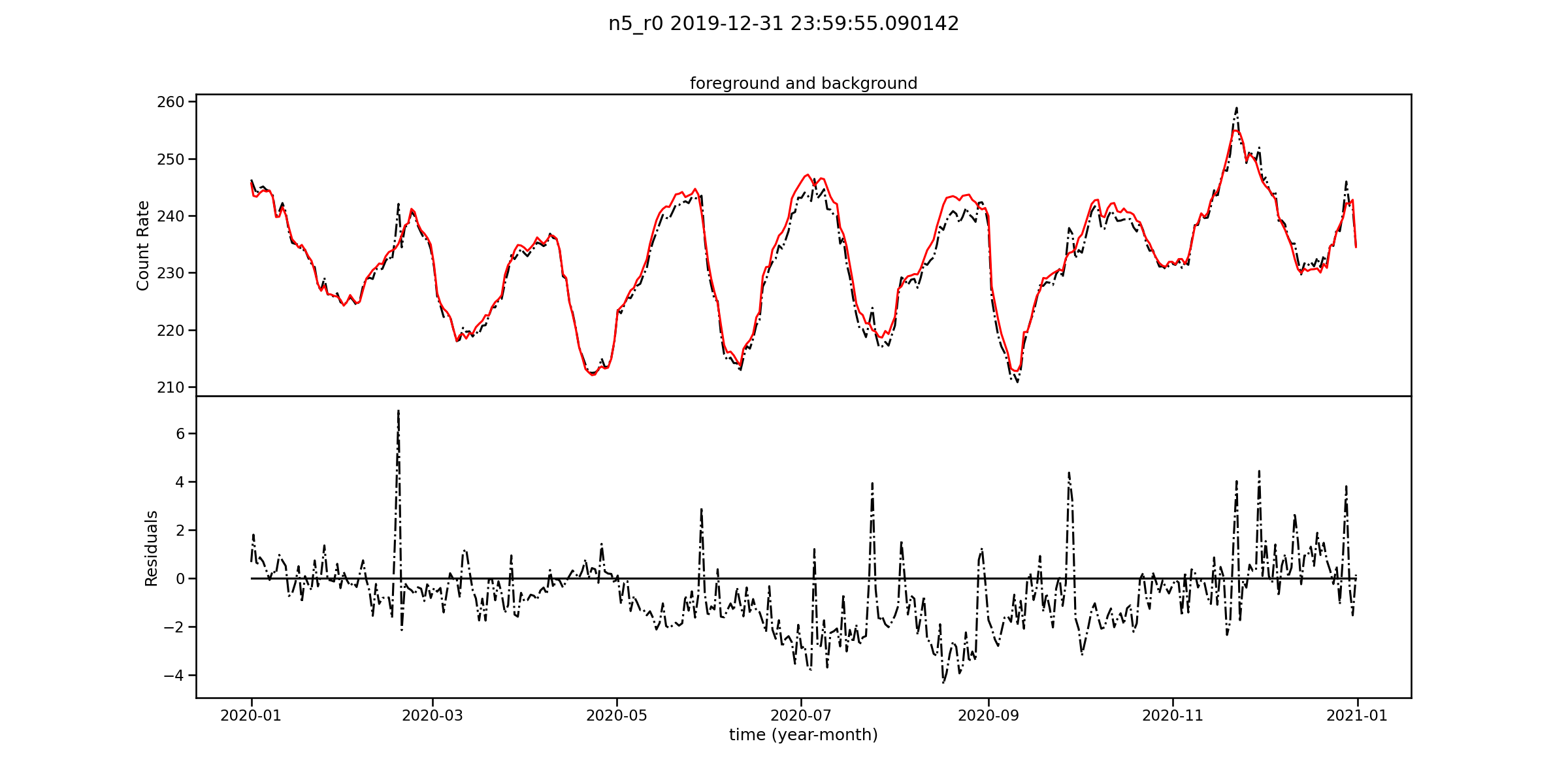
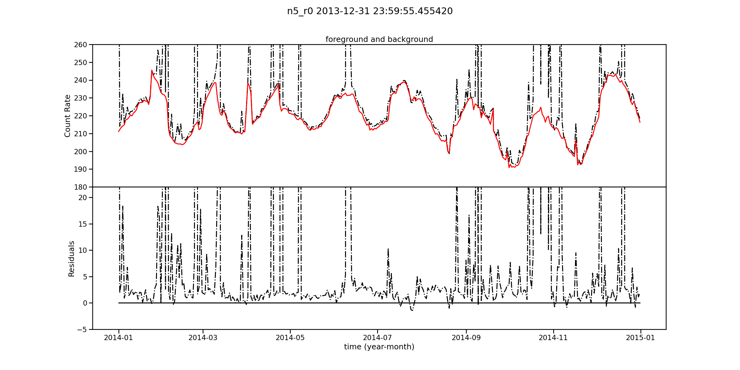
Hermes Pathfinder will be launched in 2024 that is near the next solar maximum forecast in 2025 Oceanic and Administration [2019], Biesecker and Upton [2019]. This analysis is interesting because reveals what background is expected and how the NN background estimation performs in the two periods. The most sensitive detector for the solar activity is the Sun-facing n5 Meegan et al. [2009]. In this analysis are considered background binned in a GBM period orbits (about 96m) and 16 GBM period orbits, for range 0, the most sensitive for solar flares, in the year of the last solar minima, 2014, and the local minima, 2020. The Figures 12, 13, 15 and 11, 14 are obtained considering respectively years 2014 and 2020, a NN per each year is trained. One orbit time binning for 2020 11 and 2014 13 are not comparable due to the high values of the latter but if we zoom the estimated background part we see a comparable counts rate value 12. The same reasoning applies for 16 orbits in 2020 14 and 2014 15. In Table 9 are presented the performance of the background estimation for the year 2014 and 2020. If we use a more robust metric than MAE, such MeAE, we can conclude that the estimations have comparable performance, so the the training procedure of the NN is not influenced by a huge solar activity.

Some reference for the solar cycle prediction can be found in Hathaway et al. [1994], Upton and Hathaway [2018], Bhowmik and Nandy [2018]. For evaluation purposes, the Median Absolute Error (MeAE)

$$\text{MeAE}(x,y)=\text{median}(\{\mid y_{i}-x_{i}\mid\})$$

is a robust metric against the outliers.

Figure 11: The background estimation in year 2020 for detector n5 (Sun-facing) in the energy range r0. The count rates with a time bin of 4.096s are the averaged over 1 period orbit (96m).

Figure 12: The background estimation in year 2014 for detector n5 (Sun-facing) in the energy range r0. The count rates with a time bin of 4.096s are the averaged over 1 period orbit (96m). A zoom-in is applied to avoid the outliers shown in Figure 13.

Figure 13: The background estimation in year 2014 for detector n5 (Sun-facing) in the energy range r0. The solar activity in this year is tremendously high. The count rates with a time bin of 4.096s are the averaged over 1 period orbit (96m).

Figure 14: The background estimation in year 2020 for detector n5 (Sun-facing) in the energy range r0. The count rates with a time bin of 4.096s are the averaged over 16 period orbits ($25.6$h).

Figure 15: The background estimation in year 2014 for detector n5 (Sun-facing) in the energy range r0. The count rates with a time bin of 4.096s are the averaged over 16 period orbits ($25.6$h).

year	MAE train	MAE test	MeAE train	MeAE test
2014	10.601	10.467	3.940	3.944
2020	4.897	4.914	3.901	3.909

Table 9: For each year are presented the metrics averaged per detector and range.

Appendix D Interesting events

Figure 16: Lightcurve and localization for id 1. The Sun is located under the purple spot. We classify this event as SF.

Figure 17: Lightcurve and localization for id 2. The Sun is located under the purple spot. We classify this event as SF.

Figure 18: Lightcurve and localization for id 3. Because of its location near the galactic plane and the Earth’s horizon, we could classify this event as TGF or GF.

Figure 19: Lightcurve and localization for id 4. We classify this event as a GRB.

Figure 20: Lightcurve and localization for id 5. We classify this event as a GRB.

Figure 21: Lightcurve and localization for id 6. We could classify this event as a GRB or, because of its proximity to the galactic plane, a GF.

Figure 22: In the first two figures, the lightcurve and localization for id 7 are shown. The third one shows where the GBM satellite is located on Earth. Local Particles events like LOCLPAR1905205 and LOCLPAR1904085 have occurred in this region. We classify this event as uncertain.

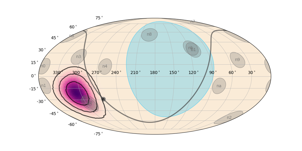
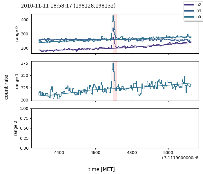
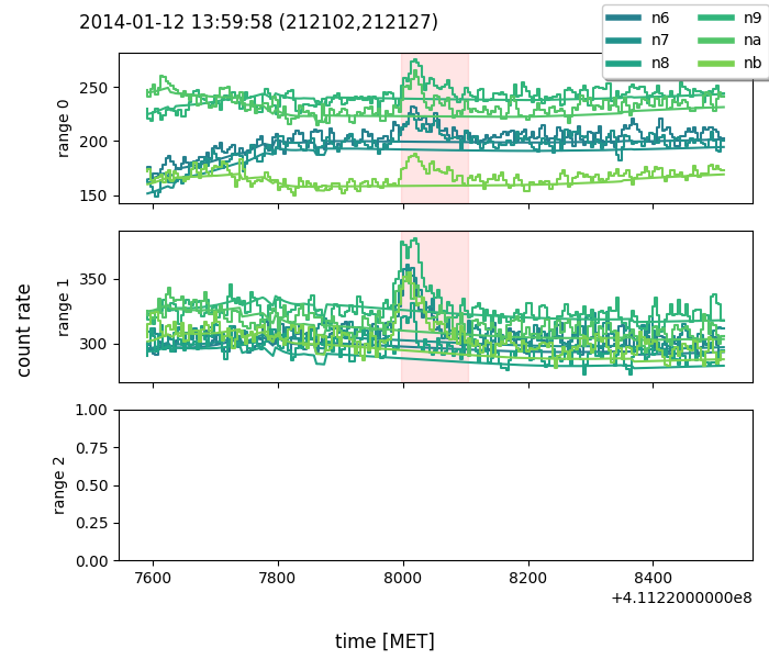
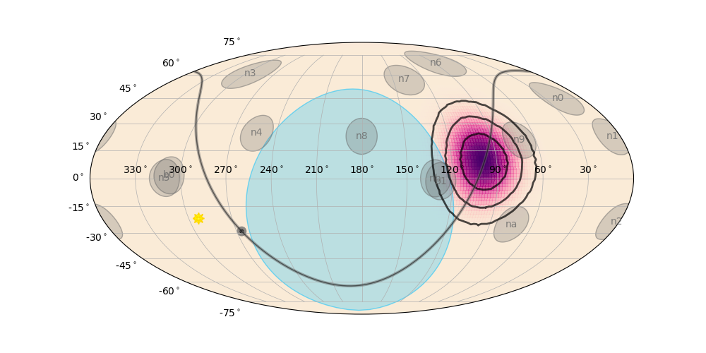
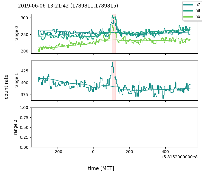
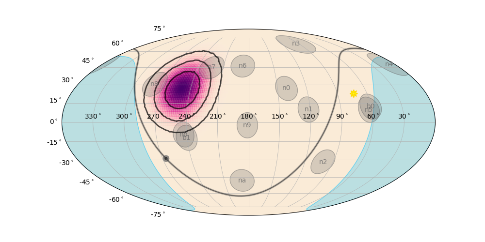
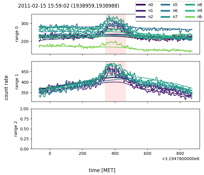
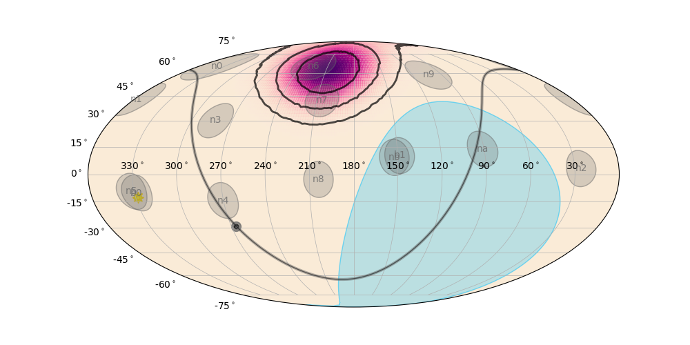
Appendix E Catalog tables

Table 10: Catalog of the unknown events for the three periods analysed. # is an incremental identifier for the events, ID is composed by the referring period and the identifier for its period (YYYY_ID). In catalog_triggers are reported “UNKNOWN: tentative transient class(es)”. $S_{r0}$, $S_{r1}$, $S_{r2}$, are the consistency of the signal for the energy range r0, r1 and r2, respectively. For the tentative transient classes are considered Gamma-Ray Bursts (GRB), Solar Flares (SF) — where the localisation of the event is near the Sun and the trigger time aligns with the GOES X-ray satellite data lightcurve peaks —, Galactic X-ray flash (GF) — where the localisation of the event is near the Galactic Plane —, Terrestial Gamma Flashes (TGF) — where the localisation of the event is near the Earth’s horizon —, Uncertain (UNC), Uncertain but resembling Local Particles (UNC(LP)). In the last column CE is reported the classification of the event, Robust (R) where more than 1 detector and more than 1 energy range is triggered, Solid (S) more than 1 detector but only 1 energy range is triggered, Probable (P) in all other cases. The events with a * in the ID are reported in table 8.

#	ID	Trigger time	T (s)	Detectors triggered	Catalog trigger name	S r0	S r1	S r2	CE
1	2010_1	2010-11-02 14:16:36	8.19	n2	UNKNOWN: GRB/GF	3.99	3.38	0	P
6	2010_6	2010-11-11 13:04:23	32.77	n2	UNKNOWN: GRB	4.29	5.81	0	P
7	2010_7*	2010-11-11 18:58:17	16.38	n2 n4 n5	UNKNOWN: SF	$>10$	4.57	0	R
10	2010_10	2010-11-12 23:46:52	19.73	n1	UNKNOWN: GRB/GF	0	9.18	5.31	P
14	2010_14	2010-11-22 13:23:34	8.19	n5 nb	UNKNOWN: UNC(LP)/GRB	0	7.45	5.41	R
33	2010_34	2010-12-28 18:22:27	106.50	na	UNKNOWN: TGF	0	8.08	0	P
38	2010_40	2011-01-16 11:40:21	20.48	n2 n5	UNKNOWN: GRB	0	5.36	0	S
44	2010_50	2011-01-31 15:52:43	8.19	n5 n6 nb	UNKNOWN: UNC(LP)	0	7.08	4.27	R
47	2010_53	2011-02-04 22:17:06	16.38	n6 n9	UNKNOWN: UNC(LP)	$>10$	7.85	0	R
48	2010_54	2011-02-04 23:07:13	102.40	n0 n3 n4 n5 n6 n7 n8	UNKNOWN: UNC(LP)	$>10$	$>10$	0	R
50	2010_56	2011-02-06 18:08:11	28.67	n8 nb	UNKNOWN: GRB	5.64	6.83	0	R
52	2010_59	2011-02-09 04:08:03	16.86	na	UNKNOWN: GRB/TGF	0	6.08	0	P
56	2010_63	2011-02-13 17:43:34	569.35	n0 n1 n2 n3 n4 n5	UNKNOWN: SF	$>10$	9.17	0	R
62	2010_70	2011-02-15 12:46:47	32.77	n0 n1 n3	UNKNOWN: GRB	0	8.48	0	S
63	2010_71*	2011-02-15 15:59:02	118.79	n0 n1 n2 n5 n6 n7 n8 n9 nb	UNKNOWN: UNC(LP)	$>10$	$>10$	0	R
67	2010_75	2011-02-16 17:31:41	233.48	n0 n1 n2 n6 n7 n8	UNKNOWN: UNC(LP)	0	$>10$	0	S
71	2010_79	2011-02-18 13:01:50	111.48	n0 n1 n2 n3 n4 n5 na	UNKNOWN: SF	$>10$	$>10$	3.63	R
72	2010_80	2011-02-18 14:07:48	8.19	n0 n1 n2 n3 n4 n5	UNKNOWN: SF	$>10$	3.78	0	R
73	2014_0	2014-01-01 03:21:00	147.46	n0 n1 n2 n3 n4 n5 n6 n7 n9 na nb	UNKNOWN: UNC(LP)	0	$>10$	$>10$	R
95	2014_26	2014-01-05 01:18:47	204.80	n0 n1 n2 n3 n5 n6 n7 n8 n9	UNKNOWN: UNC(LP)/GRB	$>10$	$>10$	0	R
97	2014_28	2014-01-05 16:04:17	73.73	n0 n1 n2 n3 n4 n5 n6 n7 n8 nb	UNKNOWN: UNC	0	$>10$	$>10$	R
98	2014_29	2014-01-06 00:53:53	593.93	n0 n1 n2 n3 n4 n5 n6 n7 n8 n9 na nb	UNKNOWN: UNC(LP)	$>10$	$>10$	$>10$	R
101	2014_34	2014-01-07 18:40:36	581.64	n0 n1 n2 n3 n4 n5	UNKNOWN: SF	$>10$	$>10$	$>10$	R
102	2014_35	2014-01-07 18:51:31	12.29	n0 n1 n3	UNKNOWN: SF	$>10$	6.96	0	R
107	2014_42	2014-01-08 19:27:13	16.38	n4	UNKNOWN: TGF	0	4.67	0	P
108	2014_51	2014-01-09 22:36:09	20.48	n7 nb	UNKNOWN: GRB/TGF	0	4.73	3.8	R
111	2014_54	2014-01-10 22:26:58	126.98	n0 n1 n2 n3 n4 n5 n6 n7 n8 n9 na nb	UNKNOWN: UNC(LP)	0	$>10$	$>10$	R
112	2014_55	2014-01-10 22:42:45	319.49	n0 n1 n2 n3 n4 n5 n6 n7 n8 n9 na	UNKNOWN: UNC(LP)	$>10$	$>10$	0	R
113	2014_56	2014-01-12 12:04:27	8.19	n4	UNKNOWN: GF/GRB	0	3.65	0	P
114	2014_57*	2014-01-12 13:59:58	102.40	n6 n7 n8 n9 na nb	UNKNOWN: GF/TGF	$>10$	$>10$	0	R
117	2014_61	2014-01-13 20:37:08	45.06	n3 n4 na	UNKNOWN: GRB/TGF	9.52	$>10$	0	R
118	2014_62	2014-01-14 20:08:58	143.36	n0 n2 n3 n4 n5 n6 n7 n8 n9 na nb	UNKNOWN: UNC(LP)	$>10$	$>10$	$>10$	R
120	2014_64	2014-01-16 08:34:49	16.38	n0 n1 n3 n4 n8 n9 nb	UNKNOWN: GF	$>10$	$>10$	6.71	R
122	2014_67	2014-01-18 17:51:57	8.19	n2 nb	UNKNOWN: GRB/TGF	0	5.52	4.39	R
123	2014_68	2014-01-18 23:59:49	16.38	n2 n5	UNKNOWN: GRB	7.44	7.78	0	R
124	2014_70	2014-01-19 08:53:20	12.29	n5 nb	UNKNOWN: TGF/GF/GRB	0	6.47	4.07	R
125	2014_71	2014-01-19 17:41:35	114.69	n0 n1 n2 n3 n4 n5 n6 n7 n8 n9 na nb	UNKNOWN: UNC(LP)	8.07	$>10$	$>10$	R
126	2014_72	2014-01-19 17:57:01	188.42	n2 n3 n4 n5 n6 n7 n8 n9 na nb	UNKNOWN: UNC(LP)	$>10$	$>10$	0	R
127	2014_73	2014-01-21 15:59:44	4.10	nb	UNKNOWN: GRB	0	3.06	0	P
130	2014_77	2014-01-24 15:14:16	176.13	n0 n1 n2 n3 n4 n5 n6 n7 n8 n9 na nb	UNKNOWN: UNC(LP)	0	$>10$	$>10$	R
131	2014_78	2014-01-25 18:55:46	8.19	n0 n3 n4	UNKNOWN: GRB/GF	4.91	6.04	0	R
134	2014_81*	2014-01-27 05:21:12	32.77	n0 n1 n2 n3 n4 n5 n8 nb	UNKNOWN: SF	$>10$	9.7	0	R
136	2014_83	2014-01-28 01:28:34	4.10	n4 n5	UNKNOWN: SF/GRB	8.96	4.51	0	R
140	2014_88	2014-01-28 12:43:39	12.29	n1 n2 n3 n4 n5	UNKNOWN: SF	$>10$	2.89	2.39	R
145	2014_93	2014-01-29 12:46:45	163.84	n0 n1 n2 n3 n4 n5 n6 n7 n8 n9 na nb	UNKNOWN: UNC(LP)	8.72	$>10$	$>10$	R
151	2014_99	2014-02-01 01:24:58	47.10	n0 n1 n2 n3 n4 n5 n8 nb	UNKNOWN: SF	$>10$	7.84	0	R
152	2014_101	2014-02-01 07:18:31	237.57	n0 n1 n2 n3 n4 n5	UNKNOWN: SF	$>10$	$>10$	0	R
155	2014_104	2014-02-13 01:37:19	368.65	n0 n1 n2 n3 n4 n5	UNKNOWN: SF	$>10$	$>10$	$>10$	R
160	2014_116	2014-02-14 02:54:08	139.27	n0 n1 n2 n3 n4 n5	UNKNOWN: SF	$>10$	$>10$	6.23	R
165	2014_121	2014-02-15 06:23:21	12.29	n6 n9	UNKNOWN: GF/GRB	4.7	4.48	0	R
166	2014_124	2014-02-16 00:23:41	888.85	n3 n4 n5 n6 n7 n8 nb	UNKNOWN: UNC(LP)	$>10$	$>10$	0	R
167	2014_125	2014-02-16 02:54:45	299.01	n0 n1 n2 n3 n4 n5 n6 n7 n8 n9 na nb	UNKNOWN: UNC(LP)	$>10$	$>10$	0	R
168	2014_126	2014-02-16 03:16:11	65.54	n1 n2 n3 n4 n5 n6 n9 na	UNKNOWN: GRB/UNC	0	$>10$	9.68	R
169	2014_127	2014-02-16 03:28:45	40.96	n0 n1 n7	UNKNOWN: GF	5.49	8.09	0	R
170	2014_128	2014-02-16 04:29:47	16.38	n0 n1 n2 n3 n4 n5 n6 n7 n8 n9 na nb	UNKNOWN: UNC(LP)	$>10$	$>10$	0	R
171	2014_129	2014-02-16 04:31:09	548.87	n0 n1 n2 n3 n4 n5 n6 n7 n8 n9 na nb	UNKNOWN: UNC(LP)	$>10$	$>10$	0	R
174	2014_132	2014-02-17 01:41:56	20.48	n0 n1 n2 n3 n5 n6 n7 n8 n9	UNKNOWN: GF/UNC(LP)	$>10$	$>10$	0	R
175	2014_133	2014-02-17 03:06:02	151.55	n0 n1 n2 n3 n4 n5 n6 n7 n8 n9 na nb	UNKNOWN: UNC(LP)	0	$>10$	$>10$	R
177	2014_138	2014-02-18 12:27:19	4.10	nb	UNKNOWN: GRB	0	3.05	0	P
178	2014_139	2014-02-18 23:06:28	172.04	n0 n1 n2 n5 n8 n9 na nb	UNKNOWN: UNC(LP)	$>10$	$>10$	$>10$	R
179	2014_140	2014-02-19 00:32:33	12.29	n0 n1 n2 n3 n4 n5	UNKNOWN: SF	$>10$	8.24	0	R
182	2014_144	2014-02-19 22:57:13	118.79	n0 n1 n3 n4 n5 n6 n7 n8 n9 na nb	UNKNOWN: UNC(LP)	$>10$	$>10$	0	R
183	2014_145	2014-02-19 23:49:23	90.11	n4	UNKNOWN: UNC(LP)/TGF	$>10$	9.12	0	P
184	2014_147	2014-02-20 12:25:01	12.29	n0 n1 n2 n3 n4 n5 n6 n7 n8 n9 na nb	UNKNOWN: UNC(LP)	$>10$	$>10$	0	R
185	2014_148	2014-02-20 22:48:09	126.98	n0 n1 n2 n3 n4 n5 n7 n8 n9 na nb	UNKNOWN: UNC(LP)	$>10$	$>10$	0	R
186	2014_149	2014-02-21 00:48:43	45.06	n2 n3 n5 n6 n8 n9 nb	UNKNOWN: GRB/GF	0	$>10$	9.67	R
187	2014_150	2014-02-21 01:03:36	270.34	n0 n1 n2 n3 n4 n5 n6 n7 n8 na	UNKNOWN: UNC(LP)	$>10$	$>10$	0	R
188	2014_151	2014-02-21 22:39:25	4.10	n9	UNKNOWN: GRB	0	3.28	0	P
189	2014_152	2014-02-22 00:37:51	155.65	n0 n1 n2 n3 n4 n5 n6 n7 n8 n9 na nb	UNKNOWN: UNC(LP)	0	$>10$	$>10$	R
190	2014_153	2014-02-23 06:02:32	401.42	n0 n1 n2 n3 n4 n5 n6 n7	UNKNOWN: SF	$>10$	$>10$	$>10$	R
192	2014_155	2014-02-23 18:14:59	503.82	n0 n1 n3 n4 n5 n8 n9	UNKNOWN: SF	$>10$	$>10$	9.67	R
193	2014_156	2014-02-23 19:49:32	589.83	n0 n1 n2 n3 n4 n5 n7 n8	UNKNOWN: UNC(LP)	$>10$	$>10$	0	R
194	2014_157	2014-02-23 20:38:16	77.83	n2 na	UNKNOWN: TGF/GRB	7.96	8.92	0	R
195	2014_158	2014-02-23 21:28:07	606.22	n0 n1 n3 n4 n5 n8	UNKNOWN: UNC(LP)	$>10$	$>10$	0	R
196	2014_159	2014-02-23 21:38:17	32.77	n3 n4 n5 n8	UNKNOWN: UNC(LP)	$>10$	$>10$	0	R
197	2014_160	2014-02-23 22:19:39	139.27	n0 n3 n4 n5 n6 n7 n8 n9 na nb	UNKNOWN: UNC(LP)	$>10$	$>10$	0	R
199	2014_163	2014-02-24 09:37:28	8.19	n0 n1 n2 n3 n4 n5	UNKNOWN: SF	$>10$	5.75	0	R
200	2014_164	2014-02-24 11:15:00	135.17	n2 n4 n5	UNKNOWN: SF	$>10$	$>10$	0	R
203	2014_167	2014-02-24 22:10:05	126.98	n0 n1 n2 n4 n5 n8 na nb	UNKNOWN: UNC(LP)	$>10$	$>10$	0	R
210	2014_176	2014-02-25 22:20:16	81.92	n2 n5 n6 n8 n9 na nb	UNKNOWN: UNC(LP)	0	$>10$	$>10$	R
211	2014_177	2014-02-25 22:33:47	131.07	n4 n5	UNKNOWN: GF/GRB	7.63	9.78	4.88	R
216	2014_184	2014-02-27 19:09:13	942.09	n0 n1 n2 n3 n4 n5 n6 n7 n8	UNKNOWN: SF	$>10$	$>10$	$>10$	R
217	2014_185	2014-02-27 19:58:42	204.80	n1 n2 n4 n7 n8 n9 na nb	UNKNOWN: GRB/TGF	$>10$	$>10$	0	R
218	2014_186	2014-02-27 20:48:00	131.07	n0 n1 n2 n3 n4 n5 n6	UNKNOWN: SF	$>10$	$>10$	8.03	R
219	2014_187	2014-02-27 20:50:23	593.93	n0 n1 n2 n3 n4 n5 n6 n7 n8	UNKNOWN: SF	$>10$	$>10$	$>10$	R
220	2014_189	2014-02-27 22:25:42	581.64	n0 n1 n2 n3 n4 n5 n6 n7 n8 n9	UNKNOWN: SF	$>10$	$>10$	9.82	R
221	2014_190	2014-02-27 23:15:57	499.72	n0 n1 n2 n3 n4 n5 n6 n7 n8 n9 na nb	UNKNOWN: UNC(LP)	$>10$	$>10$	$>10$	R
222	2014_191	2014-02-27 23:25:46	8.19	n0 n1 n2 n3 n4 n5 n8 na nb	UNKNOWN: UNC(LP)	$>10$	$>10$	7.14	R
224	2014_193	2014-02-28 20:25:58	4.10	n0	UNKNOWN: GRB	0	3.68	0	P
225	2019_0	2019-03-01 09:28:28	8.19	n6	UNKNOWN: UNC(LP)	0	3.63	0	P
228	2019_3	2019-03-06 06:45:30	77.83	n1 n4 n5 n6 n7 n8 n9 na nb	UNKNOWN: UNC(LP)	$>10$	$>10$	7.49	R
234	2019_9	2019-03-15 05:09:11	61.44	n6 n9	UNKNOWN: GRB	7.62	8.71	0	R
236	2019_11	2019-03-17 01:08:06	12.29	nb	UNKNOWN: GRB	3.97	3.84	0	P
246	2019_21	2019-03-27 06:36:04	8.19	n1	UNKNOWN: GRB	0	3.4	0	P
249	2019_24	2019-04-04 12:24:17	49.15	n0 n1 n2 n3 n5	UNKNOWN: SF/GRB	9.19	$>10$	0	R
250	2019_25*	2019-04-04 13:08:07	8.19	n9 na	UNKNOWN: GRB	0	4.93	0	S
251	2019_26	2019-04-04 13:45:40	102.40	n0 n1 n2 n3 n4 n5 n6 n7 n8 n9 na nb	UNKNOWN: UNC(LP)	$>10$	$>10$	0	R
261	2019_36	2019-04-20 15:08:24	69.63	n4 n8	UNKNOWN: GRB/GF	0	9.75	0	S
262	2019_37*	2019-04-20 22:32:56	16.38	n6 n7 n8 n9 nb	UNKNOWN: GRB	$>10$	8.4	0	R
266	2019_42	2019-04-28 00:16:26	61.44	n0 n1 n2 n3 n5 n6 n7 n8 n9 nb	UNKNOWN: UNC(LP)	$>10$	$>10$	0	R
275	2019_51	2019-05-07 17:15:13	7.42	na	UNKNOWN: TGF	0	4.85	0	P
282	2019_58	2019-05-14 07:38:41	8.19	na	UNKNOWN: TGF	0	3.09	0	P
283	2019_59	2019-05-14 10:31:29	196.61	n0 n2 n3 n4 n5 n6 n7 n8 n9 na nb	UNKNOWN: UNC(LP)	$>10$	$>10$	0	R
284	2019_60	2019-05-14 11:59:58	507.91	n0 n1 n2 n3 n4 n5 n6 n7 n8 n9 na nb	UNKNOWN: UNC(LP)	$>10$	$>10$	0	R
285	2019_61	2019-05-14 13:45:47	569.35	n0 n1 n2 n3 n4 n5 n6 n7 n8 n9 na nb	UNKNOWN: UNC(LP)	$>10$	$>10$	0	R
287	2019_63	2019-05-15 16:04:20	16.38	n4	UNKNOWN: GRB	4.9	4.03	0	P
290	2019_66	2019-05-20 05:34:01	20.48	n7 n9 na nb	UNKNOWN: GRB	5.61	8.58	0	R
292	2019_68	2019-05-24 11:15:53	24.58	n3 n7	UNKNOWN: GRB	0	6.04	0	S
293	2019_69	2019-05-28 23:32:56	16.38	n4	UNKNOWN: GRB/TGF	3.54	3.91	0	P
301	2019_77*	2019-06-06 13:21:42	16.38	n7 n8 nb	UNKNOWN: GRB/GF	9.12	6.4	0	R
304	2019_80	2019-06-08 20:22:43	8.19	n0 n1 n2 n3 n4 n6 n7 n8 n9 na nb	UNKNOWN: UNC(LP)	$>10$	$>10$	0	R
305	2019_81	2019-06-08 20:23:03	626.70	n0 n1 n2 n3 n4 n5 n6 n7 n8 n9 na nb	UNKNOWN: UNC(LP)	$>10$	$>10$	0	R
318	2019_94	2019-06-28 04:23:34	8.19	n8	UNKNOWN: GRB	0	3.4	0	P
320	2019_96	2019-07-02 15:52:26	8.19	n3	UNKNOWN: GRB	0	3.15	0	P

Table 11: Catalog of the known events for the three periods analysed. # is an incremental identifier for the events, ID is composed by the referring period and the identifier for its period (YYYY_ID). In catalog_triggers are reported the name of the event in the Fermi/GBM trigger catalog. $S_{r0}$, $S_{r1}$, $S_{r2}$, are the consistency of the signal for the energy range r0, r1 and r2, respectively. In the last column CE is reported the classification of the event, Robust (R) where more than 1 detector and more than 1 energy range is triggered, Solid (S) more than 1 detector but only 1 energy range is triggered, Probable (P) in all other cases.

#	ID	Trigger time	T (s)	Detectors triggered	Catalog trigger name	S r0	S r1	S r2	CE
0	2010_0	2010-11-01 21:34:05	34.81	n3 n4 n5	GRB101101899	5.54	8.51	0	R
2	2010_2	2010-11-02 20:10:09	41.47	n6 n7 n8 n9 nb	GRB101102840	5.9	$>10$	0	R
3	2010_3	2010-11-03 12:13:28	114.69	n0 n1 n2 n3 n4 n5 n9 na nb	SFLARE10110350	$>10$	$>10$	0	R
4	2010_4	2010-11-04 19:26:16	4.43	n2	GRB101104810	0	3.22	0	P
5	2010_5	2010-11-07 00:16:24	341.51	n0 n1 n3 n4 n5	GRB101107011	8.84	$>10$	0	R
8	2010_8	2010-11-12 22:10:31	17.92	n2 n5	GRB101112924	5.36	7.77	0	R
9	2010_9	2010-11-12 23:36:52	96.26	n3 n6 n7 n8	GRB101112984	$>10$	$>10$	0	R
11	2010_11	2010-11-13 11:35:33	202.24	n0 n1 n2 n6 n7 n8 n9 na nb	GRB101113483	$>10$	$>10$	0	R
12	2010_12	2010-11-14 17:53:19	229.38	n2 n4 n5 n6 n7 n9 na nb	TRANSNT1011147	$>10$	$>10$	0	R
13	2010_13	2010-11-17 11:54:42	108.54	n6 n7 n8 na nb	GRB101117496	$>10$	$>10$	4.04	R
15	2010_15	2010-11-23 22:52:10	204.80	n0 n1 n2 n5 n6 n7 n8 n9 na nb	GRB101123952	$>10$	$>10$	$>10$	R
16	2010_16	2010-11-26 04:44:26	112.13	n3 n4 n5 n6 n7 n8 n9 na nb	GRB101126198	$>10$	$>10$	7.12	R
17	2010_18	2010-11-27 02:27:34	45.06	n6 n7 n9 nb	GRB101127102	6.34	$>10$	0	R
18	2010_19	2010-12-01 10:01:49	108.03	n0 n1 n2 n4 n5 n7 n8 n9 na nb	GRB101201418	$>10$	$>10$	4.87	R
19	2010_20	2010-12-06 00:52:19	61.70	n0 n1 n2 n9 na	GRB101206036	7.17	$>10$	0	R
20	2010_21	2010-12-07 12:51:46	94.21	n0 n1 n2 n3 n4 n5 n6 n7	GRB101207536	$>10$	$>10$	0	R
21	2010_22	2010-12-13 20:22:28	12.58	n0 n1 n3 n5	GRB101213849	7.4	7.26	0	R
22	2010_23	2010-12-14 23:50:09	4.10	n4	GRB101214993	0	3.12	0	P
23	2010_24	2010-12-16 17:17:48	43.30	n0 n1 n2 n3 n4 n5	GRB101216721	$>10$	$>10$	0	R
24	2010_25	2010-12-19 16:28:12	30.21	n3 n4 n6 n7 n8	GRB101219686	$>10$	$>10$	0	R
25	2010_26	2010-12-20 13:50:02	106.50	n0 n1 n2 n3 n4 n5	GRB101220576	$>10$	$>10$	0	R
26	2010_27	2010-12-20 20:44:14	45.06	n3 n4 n5 n6 n7 n8	GRB101220864	$>10$	$>10$	0	R
27	2010_28	2010-12-23 20:00:17	30.21	n3 n4	GRB101223834	4.65	7.02	0	R
28	2010_29	2010-12-24 13:53:00	57.41	n0 n1 n2 n3 n5	GRB101224578	$>10$	$>10$	0	R
29	2010_30	2010-12-24 14:43:32	30.21	n2 n5	GRB101224614	7.59	6.51	0	R
30	2010_31	2010-12-25 09:04:12	106.50	n1 n2 n3 n4 n5 n6 n7 n8 n9 na nb	GRB101225377	$>10$	$>10$	0	R
31	2010_32	2010-12-27 09:45:08	168.07	n0 n1 n2 n3 n4 n5 n6 n7 n8 n9 na nb	GRB101227406	$>10$	$>10$	0	R
32	2010_33	2010-12-27 12:51:44	58.88	n6 n7 n8 n9 nb	GRB101227536	0	$>10$	0	S
34	2010_35	2010-12-31 01:36:48	108.03	n0 n1 n2 n6 n7 n8 n9 na nb	GRB101231067	$>10$	$>10$	0	R
35	2010_36	2011-01-05 21:02:32	134.15	n0 n1 n6 n7 n8 n9 na nb	GRB110105877	$>10$	$>10$	0	R
36	2010_37	2011-01-06 21:26:18	25.09	n9 na nb	GRB110106893	0	8.16	0	S
37	2010_39	2011-01-07 21:15:03	146.43	n0 n1 n2 n5	GRB110107886	$>10$	$>10$	0	R
39	2010_41	2011-01-17 15:01:25	46.59	n6 n7 n9 na nb	GRB110117626	0	$>10$	0	S
40	2010_42	2011-01-19 22:20:59	214.53	n0 n1 n2 n3 n4 n5 n6 n7 na	GRB110119931	$>10$	$>10$	0	R
41	2010_43	2011-01-20 15:59:35	211.14	n0 n1 n2 n4 n5 n6 n7 n8 n9 na nb	GRB110120666	7.87	$>10$	9.93	R
42	2010_46	2011-01-23 19:17:42	386.57	n0 n1 n2 n3 n4 n5 n6 n7 na	GRB110123804	$>10$	$>10$	$>10$	R
43	2010_49	2011-01-30 05:31:55	12.80	n7 n8 nb	GRB110130230	4.24	6.14	0	R
45	2010_51	2011-02-01 09:35:09	17.92	n4	GRB110201399	0	4.4	0	P
46	2010_52	2011-02-04 04:17:10	38.40	n0 n3 n4 n5	GRB110204179	7.9	$>10$	0	R
49	2010_55	2011-02-05 14:07:16	161.79	n5	GRB110205588	0	6.05	0	P
51	2010_57	2011-02-07 11:17:51	16.38	n3 n4	GRB110207470	0	5.23	0	S
53	2010_60	2011-02-10 06:56:19	225.28	n0 n1 n2 n3 n4 n5 n6 n7 n8 nb	SFLARE11021028	$>10$	$>10$	0	R
54	2010_61	2011-02-13 05:17:13	98.82	n1 n2 n3 n4 n5 n6 n7 n8 na nb	GRB110213220	$>10$	$>10$	0	R
55	2010_62	2011-02-13 17:33:04	584.52	n0 n1 n2 n3 n4 n5 n6 na	SFLARE11021373	$>10$	$>10$	$>10$	R
57	2010_64	2011-02-14 17:24:26	540.68	n0 n1 n2 n3 n4 n5 n6	SFLARE11021472	$>10$	$>10$	5.33	R
58	2010_65	2011-02-14 19:26:52	237.57	n0 n1 n2 n3 n4 n5 n6 n7 n8 n9 na nb	SFLARE11021481	$>10$	$>10$	0	R
59	2010_66	2011-02-15 01:48:19	447.50	n0 n1 n2 n3 n4 n5 n6 n7 n8 n9 na nb	SFLARE11021507	$>10$	$>10$	$>10$	R
60	2010_68	2011-02-15 03:09:16	61.44	n1 n2 n3 n4 n5 na nb	SFLARE11021513	$>10$	$>10$	0	R
61	2010_69	2011-02-15 07:57:42	106.50	n0 n1 n2 n3 n4 n5 n8	SFLARE11021533	$>10$	$>10$	0	R
64	2010_72	2011-02-16 01:36:25	114.69	n0 n1 n2 n3 n4 n5 n6 n7 n8 n9 na nb	SFLARE11021606	$>10$	$>10$	0	R
65	2010_73	2011-02-16 07:41:09	155.65	n2 n4 n5	SFLARE11021631	$>10$	5.46	0	R
66	2010_74	2011-02-16 14:23:21	164.00	n0 n1 n2 n3 n4 n5 n7 n8 n9 na nb	SFLARE11021660	$>10$	$>10$	2.48	R
68	2010_76	2011-02-17 12:35:08	40.96	n0 n1 n2 n3 n4 n5 n9 na nb	SFLARE11021752	$>10$	8.17	0	R
69	2010_77	2011-02-17 14:10:53	12.29	n1 na	GRB110217591	0	4.74	0	S
70	2010_78	2011-02-18 06:30:43	117.76	n0 n1 n2 n3 n4 n5 n9 na nb	SFLARE11021827	$>10$	$>10$	0	R
74	2014_1	2014-01-01 18:44:35	445.44	n0 n1 n2 n3 n4 n5 n9 na	SFLARE14010178	$>10$	$>10$	$>10$	R
75	2014_2	2014-01-01 23:10:59	20.48	n0 n1 n2 n3 n4 n5 n8	SFLARE14010196	$>10$	6.91	0	R
76	2014_3	2014-01-02 02:02:21	22.50	n0 n1 n2 n3 n4 n5	SFLARE14010208	$>10$	7.24	0	R
77	2014_4	2014-01-02 02:29:16	302.08	n0 n1 n2 n3 n4 n5 n7 n8 n9 nb	SFLARE14010210	$>10$	$>10$	0	R
78	2014_5	2014-01-02 05:44:45	113.66	n0 n1 n2 n3 n4 n5 n6 n7 n8 nb	SFLARE14010224	$>10$	$>10$	0	R
79	2014_6	2014-01-02 08:43:28	89.09	n0 n1 n2 n3 n4 n5 n8 nb	SFLARE14010236	$>10$	$>10$	0	R
80	2014_7	2014-01-02 21:17:34	108.51	n0 n1 n2 n3 n4 n5 n6 n7 n8 n9 na nb	GRB140102887	$>10$	$>10$	8.43	R
81	2014_8	2014-01-02 21:43:18	102.40	n0 n1 n2 n3 n4 n5 n7 n8	SFLARE14010290	$>10$	$>10$	0	R
82	2014_12	2014-01-03 02:25:57	45.06	n0 n1 n2 n3 n4 n5 n7 n8	SFLARE14010310	$>10$	9.01	0	R
83	2014_13	2014-01-03 03:58:56	102.40	n0 n1 n2 n3 n4 n5 n6 n7 n8 nb	SFLARE14010316	$>10$	$>10$	0	R
84	2014_14	2014-01-03 12:48:39	45.25	n2 n4 n5 n9 na	SFLARE14010353	$>10$	9.64	7.17	R
85	2014_15	2014-01-03 15:17:03	12.29	n1 n2 n3 n4 n5	SFLARE14010363	$>10$	7.59	0	R
86	2014_16	2014-01-03 20:06:11	108.03	n0 n1 n2 n3 n4 n5	SFLARE14010383	$>10$	$>10$	0	R
87	2014_17	2014-01-03 21:11:59	113.66	n0 n1 n2 n3 n4 n5 n8 na nb	SFLARE14010388	$>10$	$>10$	0	R
88	2014_18	2014-01-04 10:19:09	401.41	n0 n1 n2 n3 n4 n5 n6 n7 n8 nb	SFLARE14010443	$>10$	$>10$	$>10$	R
89	2014_20	2014-01-04 17:32:08	594.45	n2 n3 n5 n6 n7 n8 n9 na nb	GRB140104731	$>10$	$>10$	0	R
90	2014_21	2014-01-04 19:05:40	121.86	n0 n1 n2 n3 n4 n5	SFLARE14010479	$>10$	$>10$	0	R
91	2014_22	2014-01-04 19:08:02	1522.65	n0 n1 n2 n3 n4 n5 n9 na	SFLARE14010479	$>10$	$>10$	$>10$	R
92	2014_23	2014-01-04 19:33:37	593.93	n0 n1 n3 n5	SFLARE14010479	$>10$	$>10$	$>10$	R
93	2014_24	2014-01-04 19:45:42	393.22	n0 n1 n3 n4 n5	SFLARE14010479	$>10$	$>10$	0	R
94	2014_25	2014-01-04 19:57:31	208.90	n4 n5	SFLARE14010479	$>10$	9.54	0	R
96	2014_27	2014-01-05 01:33:03	8.30	n9	GRB140105065	0	3.49	0	P
99	2014_31	2014-01-06 08:16:45	28.93	n2 n5	GRB140106345	5.2	7.69	0	R
100	2014_32	2014-01-06 22:45:12	145.26	n0 n1 n2 n3 n4 n5 n6 n7 n8 n9 na nb	SFLARE14010694	$>10$	$>10$	7.23	R
103	2014_36	2014-01-07 22:18:30	45.06	n0 n1 n2 n3 n4 n5 n8 nb	SFLARE14010792	$>10$	9.58	0	R
104	2014_37	2014-01-08 03:06:45	86.02	n0 n1 n2 n3 n4 n5 n7 n8 na nb	SFLARE14010813	$>10$	$>10$	0	R
105	2014_38	2014-01-08 12:57:46	55.22	n1 n2 n3 n4 n5 n8	SFLARE14010854	$>10$	$>10$	5.97	R
106	2014_40	2014-01-08 17:18:45	184.58	n0 n1 n2 n3 n4 n5 n7 n8 n9 na nb	GRB140108721	$>10$	$>10$	7.65	R
109	2014_52	2014-01-10 06:18:34	63.10	n6 n7 n8 n9 na nb	GRB140110263	6.29	$>10$	7.6	R
110	2014_53	2014-01-10 19:31:26	72.71	n8	GRB140110814	7.09	8.55	0	P
115	2014_58	2014-01-13 04:23:54	22.02	n7 n9 nb	GRB140113183	6.92	5.79	0	R
116	2014_60	2014-01-13 15:04:12	40.96	n0 n1 n2 n3 n4 n5 n8	GRB140113624	$>10$	$>10$	0	R
119	2014_63	2014-01-15 20:43:17	71.17	n2 n3 n4 n5 n6 n7 n8	GRB140115863	9.5	$>10$	0	R
121	2014_65	2014-01-17 16:06:58	110.59	n0 n1 n2 n3 n4 n5 n8	SFLARE14011767	$>10$	$>10$	0	R
128	2014_74	2014-01-22 14:19:45	9.73	n8	GRB140122597	0	3.35	0	P
129	2014_76	2014-01-24 12:38:24	171.01	n0 n1 n2 n3 n4 n5 n6 n9	GRB140124527	$>10$	$>10$	9.56	R
132	2014_79	2014-01-26 19:32:48	130.05	n3 n4 n6 n7 n8	GRB140126815	$>10$	$>10$	0	R
133	2014_80	2014-01-27 02:04:16	129.02	n0 n1 n2 n3 n4 n5 n7 n8 n9 na nb	SFLARE14012708	$>10$	$>10$	0	R
135	2014_82	2014-01-28 00:34:02	13.82	n0 n1 n2 n3 n4 n5 n7 n8 nb	SFLARE14012802	$>10$	$>10$	0	R
137	2014_85	2014-01-28 05:27:05	112.13	n0 n1 n2 n3 n4 n5 n6 n7 n8 nb	SFLARE14012822	$>10$	$>10$	0	R
138	2014_86	2014-01-28 11:34:34	287.20	n0 n1 n2 n3 n4 n5 n6 n7 n8 n9 na nb	SFLARE14012848	$>10$	$>10$	4.64	R
139	2014_87	2014-01-28 11:45:17	20.48	n0 n1 n2 n3 n4 n5	SFLARE14012848	$>10$	7.08	0	R
141	2014_89	2014-01-28 12:57:05	69.63	n0 n2 n5 n7 n9 nb	SFLARE14012853	0	$>10$	9.72	R
142	2014_90	2014-01-28 22:15:33	557.07	n0 n1 n2 n3 n4 n5	SFLARE14012892	$>10$	$>10$	7.83	R
143	2014_91	2014-01-29 03:33:07	36.86	n0 n1 n2 n3 n4 n5 n7 n8 nb	SFLARE14012914	$>10$	$>10$	0	R
144	2014_92	2014-01-29 09:40:45	16.86	n0 n1 n2 n3 n4 n5 nb	SFLARE14012940	$>10$	7.25	0	R
146	2014_94	2014-01-30 06:16:33	13.82	n0 n1 n2 n3 n4 n5 na	SFLARE14013026	$>10$	7.88	0	R
147	2014_95	2014-01-30 06:35:48	499.72	n0 n1 n2 n3 n4 n5 n6 n7 n8 n9 na nb	SFLARE14013027	$>10$	$>10$	$>10$	R
148	2014_96	2014-01-30 06:51:07	41.28	n1 n2 n3 n4 n5	SFLARE14013028	$>10$	7.65	0	R
149	2014_97	2014-01-30 07:52:24	572.43	n0 n1 n2 n3 n4 n5 n7 n8 n9 na nb	SFLARE14013033	$>10$	$>10$	8.18	R
150	2014_98	2014-01-30 08:02:25	195.61	n0 n1 n2 n3 n4 n5 na	SFLARE14013033	$>10$	$>10$	7.42	R
153	2014_102	2014-02-01 10:45:09	32.77	n0 n1 n2 n3 n4 n5 n9 na nb	SFLARE14020144	$>10$	8.37	0	R
154	2014_103	2014-02-01 18:23:09	30.72	n1 n2 n3 n4 n5	SFLARE14020176	$>10$	$>10$	0	R
156	2014_105	2014-02-13 06:05:07	156.11	n0 n1 n2 n3 n4 n5 n6 n7 n8 n9 na nb	SFLARE14021325	$>10$	$>10$	7.81	R
157	2014_106	2014-02-13 15:54:50	187.40	n0 n1 n2 n3 n4 n5	SFLARE14021366	$>10$	$>10$	5.78	R
158	2014_107	2014-02-13 19:21:29	562.70	n0 n1 n2 n3 n4 n5 n6 n7 n8 n9 na nb	GRB140213807	$>10$	$>10$	$>10$	R
159	2014_109	2014-02-13 19:33:55	1326.10	n0 n1 n2 n3 n4 n5 n6 n7 n8 n9 na nb	SFLARE14021382	$>10$	$>10$	$>10$	R
161	2014_117	2014-02-14 03:04:13	221.36	n0 n1 n2 n3 n4 n5	SFLARE14021412	$>10$	$>10$	0	R
162	2014_118	2014-02-14 04:27:53	28.67	n0 n1 n2 n3 n4 n5 n9 na nb	SFLARE14021418	$>10$	7.06	0	R
163	2014_119	2014-02-14 12:33:52	537.64	n0 n1 n2 n3 n4 n5 n7 n8	SFLARE14021452	$>10$	$>10$	8.86	R
164	2014_120	2014-02-14 16:35:36	335.88	n0 n1 n2 n3 n4 n5	SFLARE14021469	$>10$	$>10$	0	R
172	2014_130	2014-02-16 13:50:59	111.10	n0 n1 n2 n3 n4 n5 n9 na nb	SFLARE14021657	$>10$	$>10$	0	R
173	2014_131	2014-02-17 01:01:44	28.80	n0 n1 n3 n6 n9	GRB140217043	$>10$	8.74	0	R
176	2014_136	2014-02-18 10:08:43	449.54	n2 n3 n4 n5 n6 n7 n8 n9 na nb	GRB140218427	$>10$	$>10$	$>10$	R
180	2014_142	2014-02-19 19:46:34	61.70	n8 nb	GRB140219824	7.55	8.7	0	R
181	2014_143	2014-02-19 22:22:20	41.05	n0 n1 n2 n3 n4 n5	SFLARE14021993	$>10$	$>10$	0	R
191	2014_154	2014-02-23 11:53:08	41.22	n5 n6 n7 n8 n9 nb	GRB140223495	0	$>10$	0	S
198	2014_162	2014-02-24 09:10:19	4.54	n2	GRB140224382	0	3.55	0	P
201	2014_165	2014-02-24 18:55:19	38.40	n3 n4 n6 n7 n8	GRB140224788	6.35	$>10$	0	R
202	2014_166	2014-02-24 21:35:34	116.74	n0 n1 n2 n3 n4 n5 n8 na	SFLARE14022490	$>10$	$>10$	0	R
204	2014_168	2014-02-25 00:41:27	1612.29	n0 n1 n2 n3 n4 n5 n6 n7 n8 n9 na nb	SFLARE14022502	$>10$	$>10$	$>10$	R
205	2014_169	2014-02-25 01:08:27	495.63	n0 n1 n2 n3 n4 n5 n9	SFLARE14022502	$>10$	$>10$	5.21	R
206	2014_170	2014-02-25 01:16:59	434.18	n0 n1 n3 n5	SFLARE14022502	$>10$	$>10$	$>10$	R
207	2014_171	2014-02-25 01:27:26	294.92	n0 n1 n2 n3 n4 n5	SFLARE14022502	$>10$	$>10$	6.64	R
208	2014_173	2014-02-25 06:18:56	32.77	n1 n2 n3 n4 n5	SFLARE14022526	$>10$	7.66	0	R
209	2014_175	2014-02-25 15:06:38	106.82	n0 n1 n2 n3 n4 n5 n8	SFLARE14022563	$>10$	$>10$	0	R
212	2014_180	2014-02-27 05:56:09	78.24	n0 n1 n2 n3 n4 n5	SFLARE14022724	$>10$	$>10$	0	R
213	2014_181	2014-02-27 09:04:25	83.46	n0 n1 n2 n3 n4 n5 na	SFLARE14022737	$>10$	$>10$	0	R
214	2014_182	2014-02-27 10:44:42	106.59	n0 n1 n2 n3 n4 n5	SFLARE14022744	$>10$	$>10$	0	R
215	2014_183	2014-02-27 17:43:06	13.82	n0 n3 n4 n5 na	GRB140227738	$>10$	4.99	0	R
223	2014_192	2014-02-28 00:47:28	108.03	n0 n1 n2 n3 n4 n5 n6 n7 n8 n9 na nb	SFL140228033	$>10$	$>10$	0	R
226	2019_1	2019-03-03 05:45:19	88.06	n0 n1 n2 n5	GRB190303240	8.96	$>10$	0	R
227	2019_2	2019-03-04 19:37:21	9.73	n4	GRB190304818	4.4	6.29	0	P
229	2019_4	2019-03-06 22:37:42	185.86	n0 n1 n6 n7 n8 n9 na nb	GRB190306943	$>10$	$>10$	0	R
230	2019_5	2019-03-07 03:37:19	152.06	n0 n1 n2 n3 n4 n5 n9 na nb	GRB190307151	$>10$	$>10$	0	R
231	2019_6	2019-03-10 09:32:35	152.07	n0 n1 n2 n3 n4 n5 n6 n7 n8 n9 na nb	GRB190310398	$>10$	$>10$	0	R
232	2019_7	2019-03-11 14:23:37	9.73	n8	GRB190311600	0	3.36	0	P
233	2019_8	2019-03-12 10:42:13	29.18	n0 n1 n3 n4	GRB190312446	$>10$	$>10$	0	R
235	2019_10	2019-03-15 12:17:44	106.75	n0 n1 n4 n5 n6 n7 n8 n9 na nb	GRB190315512	$>10$	$>10$	4.57	R
237	2019_12	2019-03-20 01:14:21	49.15	n6 n7 n8 n9 na nb	GRB190320052	5.74	$>10$	0	R
238	2019_13	2019-03-21 14:42:05	45.42	n2 n4 n5	SFLARE19032161	$>10$	7.83	0	R
239	2019_14	2019-03-23 07:16:50	108.03	n0 n1 n6 n7 n8 n9 na nb	GRB190323303	$>10$	$>10$	5.54	R
240	2019_15	2019-03-23 21:05:18	113.15	n0 n1 n2 n3 n4 n5 n6 n7 n8 n9 na nb	GRB190323879	$>10$	$>10$	$>10$	R
241	2019_16	2019-03-24 08:21:13	114.69	n0 n1 n2 n3 n4 n5 n6 n7 n8 n9 na nb	GRB190324348	$>10$	$>10$	8.23	R
242	2019_17	2019-03-24 22:44:17	106.50	n0 n2 n6 n7 n8 n9 na nb	GRB190324947	$>10$	$>10$	6	R
243	2019_18	2019-03-25 23:58:59	341.12	n0 n1 n2 n3 n4 n5 n9 na nb	GRB190325999	$>10$	$>10$	6.87	R
244	2019_19	2019-03-26 23:24:43	41.22	n0 n1 n6 n9 na	GRB190326975	3.98	$>10$	0	R
245	2019_20	2019-03-27 02:39:13	45.57	n1 n2 n3 n4 n6 n7 n8 n9 na	GRB190327111	0	$>10$	6.32	R
247	2019_22	2019-03-30 16:39:28	108.16	n0 n1 n2 n3 n4 n5 n6 n7 n8 n9 na nb	GRB190330694	$>10$	$>10$	8.91	R
248	2019_23	2019-04-01 03:20:19	108.03	n3 n4 n5 n6 n7 n8 n9 na nb	GRB190401139	$>10$	$>10$	0	R
252	2019_27	2019-04-06 10:47:22	4.61	n3 n4	GRB190406450	5.13	4.58	0	R
253	2019_28	2019-04-06 17:52:31	103.94	n0 n2 n3 n4 n5 n6 n7	GRB190406745	$>10$	$>10$	6.23	R
254	2019_29	2019-04-07 13:48:39	12.67	n3 n6 n9	GRB190407575	4.92	7.12	0	R
255	2019_30	2019-04-07 16:07:29	20.99	n6 n7 n9 na	GRB190407672	8	8.22	0	R
256	2019_31	2019-04-08 12:51:22	363.53	n0 n1 n2 n3 n4 n5 n6 n7 n8 n9 na nb	LOCLPAR1904085	$>10$	$>10$	0	R
257	2019_32	2019-04-11 09:45:46	22.02	n0 n1 n2 n6 n8 n9 na	GRB190411407	0	$>10$	$>10$	R
258	2019_33	2019-04-11 13:53:56	79.36	n0 n1 n2 n5	GRB190411579	8.76	$>10$	0	R
259	2019_34	2019-04-15 04:09:46	112.18	n0 n1 n2 n3 n4 n5 n6 n7 n8 n9 na nb	GRB190415173	$>10$	$>10$	$>10$	R
260	2019_35	2019-04-19 09:55:40	262.53	n0 n1 n2 n3 n4 n5 n6 n7 n8 n9 na nb	GRB190419414	$>10$	$>10$	6.32	R
263	2019_38	2019-04-20 23:32:27	8.38	n6	GRB190420981	0	3.62	0	P
264	2019_39	2019-04-22 16:05:09	20.48	na nb	GRB190422670	0	6.94	0	S
265	2019_41	2019-04-22 22:56:09	183.30	n6 n7 n8 nb	GRB190422957	8.83	$>10$	0	R
267	2019_43	2019-04-28 18:48:11	62.98	n0 n1 n2 n3 n4 n5 na nb	GRB190428783	$>10$	$>10$	0	R
268	2019_44	2019-04-29 17:49:54	20.48	n9 na nb	GRB190429743	0	6.94	0	S
269	2019_45	2019-05-02 04:01:32	24.64	n0 n3 n4 n6 n7	GRB190502168	9.77	9.94	0	R
270	2019_46	2019-05-04 09:57:36	20.99	n3	GRB190504415	0	4.44	0	P
271	2019_47	2019-05-06 05:07:05	176.13	n0 n1 n2 n3 n4 n5	SFLARE19050621	$>10$	$>10$	0	R
272	2019_48	2019-05-06 13:53:21	49.15	n0 n1 n2 n3 n4 n5	SFLARE19050657	$>10$	3	0	R
273	2019_49	2019-05-06 17:47:45	89.09	n1 n2 n3 n4 n5	SFLARE19050674	$>10$	$>10$	0	R
274	2019_50	2019-05-07 06:28:19	47.62	n1 n8 n9 na	GRB190507270	5.75	9.53	0	R
276	2019_52	2019-05-07 23:16:29	108.03	n0 n1 n6 n7 n8 n9 na nb	GRB190507970	$>10$	$>10$	0	R
277	2019_53	2019-05-08 19:22:49	79.36	n6 n7 n8 nb	GRB190508808	9.3	$>10$	0	R
278	2019_54	2019-05-09 05:44:02	299.01	n0 n1 n2 n3 n4 n5 n6 n7 n8 na nb	SFL190509239	$>10$	$>10$	0	R
279	2019_55	2019-05-10 10:12:57	393.22	n1 n4 na	GRB190510430	4.03	5.44	0	R
280	2019_56	2019-05-11 07:14:26	107.01	n0 n1 n2 n3 n4 n5 n6 n7 n8 n9 na nb	GRB190511302	$>10$	$>10$	0	R
281	2019_57	2019-05-12 14:40:04	20.48	n0 n3	GRB190512611	4.72	6.05	0	R
286	2019_62	2019-05-14 21:41:40	12.29	n9	TGF190514901	6.65	5.19	0	P
288	2019_64	2019-05-17 19:30:08	62.98	n0 n1 n7 n8 n9 na nb	GRB190517813	$>10$	$>10$	0	R
289	2019_65	2019-05-19 07:24:53	145.92	n0 n1 n2 n3 n4 n5 n7 n8 n9 na nb	GRB190519309	$>10$	$>10$	0	R
291	2019_67	2019-05-20 14:21:05	150.53	n0 n1 n2 n3 n4 n5 n6 n7 n8 n9 na nb	LOCLPAR1905205	$>10$	$>10$	0	R
294	2019_70	2019-05-30 10:19:05	116.99	n0 n1 n2 n3 n4 n5 n6 n7 n8 n9 na nb	GRB190530430	$>10$	$>10$	$>10$	R
295	2019_71	2019-05-31 07:29:10	87.55	n0 n1 n2 n3 n4 n5 n9	GRB190531312	$>10$	$>10$	0	R
296	2019_72	2019-05-31 20:10:02	126.98	n0 n1 n2 n3 n4 n5 n6 n7 n8 n9 na nb	GRB190531840	$>10$	$>10$	$>10$	R
297	2019_73	2019-06-03 19:04:31	12.29	n0 n3 n4 n5	GRB190603795	7.3	6.8	0	R
298	2019_74	2019-06-04 10:42:33	108.80	n0 n1 n2 n3 n4 n5 n6 n7 n8	GRB190604446	$>10$	$>10$	$>10$	R
299	2019_75	2019-06-05 23:22:29	16.58	n4 n7 n8	GRB190605974	0	6.33	0	S
300	2019_76	2019-06-06 01:55:04	46.98	n0 n1 n2 n3 n4 n5 n9 na	GRB190606080	6.96	$>10$	5.45	R
302	2019_78	2019-06-07 01:42:46	45.31	n6 n7 n9 na nb	GRB190607071	8.88	$>10$	0	R
303	2019_79	2019-06-08 00:12:20	106.75	n6 n7 n8 n9 na nb	GRB190608009	9.44	$>10$	0	R
306	2019_82	2019-06-08 20:35:08	400.39	n0 n1 n2 n3 n4 n5 n6 n7 n8 n9 na nb	LOCLPAR1906088	$>10$	$>10$	0	R
307	2019_83	2019-06-09 07:33:36	138.24	n3 n4 n5 n6 n7 n8 n9 na nb	GRB190609315	$>10$	$>10$	$>10$	R
308	2019_84	2019-06-10 18:00:05	102.40	n0 n1 n2 n5 n6 n7 n8 n9 na nb	GRB190610750	$>10$	$>10$	0	R
309	2019_85	2019-06-11 22:47:46	178.05	n0 n1 n2 n3 n4 n5 n9	GRB190611950	$>10$	$>10$	$>10$	R
310	2019_86	2019-06-12 03:57:24	22.02	n4 n8	GRB190612165	4.6	5.27	0	R
311	2019_87	2019-06-13 04:07:21	45.06	n0 n1 n3 n8	GRB190613172	$>10$	$>10$	0	R
312	2019_88	2019-06-13 10:46:58	38.40	n3 n4 n5 n6 n7 n8 n9 nb	GRB190613449	8.28	$>10$	0	R
313	2019_89	2019-06-15 15:16:26	79.36	n4 n6 n7 n8 n9 nb	GRB190615636	8.23	$>10$	0	R
314	2019_90	2019-06-19 00:24:24	154.63	n0 n1 n3 n6 n9	GRB190619018	$>10$	$>10$	0	R
315	2019_91	2019-06-19 14:15:55	146.43	n1 n2 n3 n4 n5 n6 n7 n8 n9 na nb	GRB190619595	$>10$	$>10$	5.83	R
316	2019_92	2019-06-20 12:10:10	116.23	n0 n1 n2 n3 n4 n5 n6 n7 n8 n9 na nb	GRB190620507	$>10$	$>10$	$>10$	R
317	2019_93	2019-06-26 06:06:24	4.61	n2	GRB190626254	3.18	3.12	0	P
319	2019_95	2019-06-28 12:30:54	26.11	na nb	GRB190628521	5.32	7.16	0	R
321	2019_97	2019-07-07 06:50:04	108.03	n0 n2 n3 n4 n5 n6 n7 n8 nb	GRB190707285	$>10$	$>10$	0	R
322	2019_98	2019-07-07 07:22:58	30.72	n3 n4	GRB190707308	6.24	7.25	0	R
323	2019_99	2019-07-08 08:45:14	16.89	n3 n4 n7 n8	GRB190708365	0	6.87	0	S

References

- Woosley [1993] Stan E Woosley. Gamma-ray bursts from stellar mass accretion disks around black holes. The Astrophysical Journal, 405:273–277, 1993.
- Berger [2014] Edo Berger. Short-duration gamma-ray bursts. Annual review of Astronomy and Astrophysics, 52:43–105, 2014.
- Fiore et al. [2020] Fabrizio Fiore, Luciano Burderi, Michelle Lavagna, Roberto Bertacin, Yuri Evangelista, Riccardo Campana, Fabio Fuschino, Paolo Lunghi, Angel Monge, Barbara Negri, et al. The hermes-technologic and scientific pathfinder. In Space Telescopes and Instrumentation 2020: Ultraviolet to Gamma Ray, volume 11444, pages 214–228. SPIE, 2020.
- Fiore et al. [2021] Fabrizio Fiore, Norbert Werner, and Ehud Behar. Distributed Architectures and Constellations for -ray Burst Science. Galaxies, 9(4):120, December 2021. doi:10.3390/galaxies9040120.
- Fuschino et al. [2019] Fabio Fuschino, RICCARDO Campana, CLAUDIO Labanti, Yuri Evangelista, MARCO Feroci, L Burderi, Fabrizio Fiore, Filippo Ambrosino, G Baldazzi, P Bellutti, et al. Hermes: An ultra-wide band x and gamma-ray transient monitor on board a nano-satellite constellation. Nuclear Instruments and Methods in Physics Research Section A: Accelerators, Spectrometers, Detectors and Associated Equipment, 936:199–203, 2019.
- Evangelista et al. [2020] Yuri Evangelista, Fabrizio Fiore, Fabio Fuschino, Riccardo Campana, Francesco Ceraudo, Evgeny Demenev, Alejandro Guzman, Claudio Labanti, Giovanni La Rosa, Mauro Fiorini, et al. The scientific payload on-board the hermes-tp and hermes-sp cubesat missions. In Space Telescopes and Instrumentation 2020: Ultraviolet to Gamma Ray, volume 11444, page 114441T. International Society for Optics and Photonics, 2020.
- Fiore et al. [2022] Fabrizio Fiore, Alejandro Guzman, Riccardo Campana, and Yuri Evangelista. HERMES-Pathfinder. arXiv e-prints, art. arXiv:2210.13842, October 2022. doi:10.48550/arXiv.2210.13842.
- Evangelista et al. [2022] Y. Evangelista, F. Fiore, R. Campana, F. Ceraudo, G. Della Casa, E. Demenev, G. Dilillo, M. Fiorini, M. Grassi, A. Guzman, P. Hedderman, E. J. Marchesini, G. Morgante, F. Mele, P. Nogara, A. Nuti, R. Piazzolla, S. Pliego Caballero, I. Rashevskaya, F. Russo, G. Sottile, C. Labanti, G. Baroni, P. Bellutti, G. Bertuccio, J. Cao, T. Chen, I. Dedolli, M. Feroci, F. Fuschino, M. Gandola, N. Gao, F. Ficorella, P. Malcovati, A. Picciotto, A. Rachevski, A. Santangelo, C. Tenzer, A. Vacchi, L. Wang, Y. Xu, G. Zampa, N. Zampa, and N. Zorzi. Design, integration, and test of the scientific payloads on-board the HERMES constellation and the SpIRIT mission. In Jan-Willem A. den Herder, Shouleh Nikzad, and Kazuhiro Nakazawa, editors, Space Telescopes and Instrumentation 2022: Ultraviolet to Gamma Ray, volume 12181 of Society of Photo-Optical Instrumentation Engineers (SPIE) Conference Series, page 121811G, August 2022. doi:10.1117/12.2628978.
- Meegan et al. [2009] Charles Meegan, Giselher Lichti, PN Bhat, Elisabetta Bissaldi, Michael S Briggs, Valerie Connaughton, Roland Diehl, Gerald Fishman, Jochen Greiner, Andrew S Hoover, et al. The fermi gamma-ray burst monitor. The Astrophysical Journal, 702(1):791, 2009.
- Paciesas et al. [1999] William S Paciesas, Charles A Meegan, Geoffrey N Pendleton, Michael S Briggs, Chryssa Kouveliotou, Thomas M Koshut, John Patrick Lestrade, Michael L McCollough, Jerome J Brainerd, Jon Hakkila, et al. The fourth batse gamma-ray burst catalog (revised). The Astrophysical Journal Supplement Series, 122(2):465, 1999.
- Feroci et al. [1997] Marco Feroci, Filippo Frontera, Enrico Costa, Daniele Dal Fiume, Lorenzo Amati, L Bruca, Maria Nerina Cinti, Alessandro Coletta, P Collina, C Guidorzi, et al. In-flight performances of the bepposax gamma-ray burst monitor. In EUV, X-Ray, and Gamma-Ray Instrumentation for Astronomy VIII, volume 3114, pages 186–197. SPIE, 1997.
- Kommers [1999] Jefferson Michael Kommers. Faint gamma-ray bursts and other high-energy transients detected with BATSE. PhD thesis, Massachusetts Institute of Technology, 1999.
- Kocevski et al. [2018] D Kocevski, E Burns, A Goldstein, T Dal Canton, MS Briggs, L Blackburn, P Veres, CM Hui, R Hamburg, OJ Roberts, et al. Analysis of sub-threshold short gamma-ray bursts in fermi gbm data. The Astrophysical Journal, 862(2):152, 2018.
- Hui et al. [2017] CM Hui, MS Briggs, P Veres, and R Hamburg. Finding untriggered gamma-ray transients in the fermi gbm data. In Proceedings of the 7th International Fermi Symposium, page 129, 2017.
- Biltzinger et al. [2020] Björn Biltzinger, Felix Kunzweiler, Jochen Greiner, Kilian Toelge, and J Michael Burgess. A physical background model for the fermi gamma-ray burst monitor. Astronomy & Astrophysics, 640:A8, 2020.
- Sadeh [2019] Iftach Sadeh. Deep learning detection of transients. arXiv preprint arXiv:1902.03620, 2019.
- LeCun et al. [2015] Yann LeCun, Yoshua Bengio, and Geoffrey Hinton. Deep learning. nature, 521(7553):436–444, 2015.
- Bishop et al. [1995] Christopher M Bishop et al. Neural networks for pattern recognition. Oxford university press, 1995.
- Gendre et al. [2019] B Gendre, QT Joyce, NB Orange, G Stratta, JL Atteia, and M Boër. Can we quickly flag ultra-long gamma-ray bursts? Monthly Notices of the Royal Astronomical Society, 486(2):2471–2476, 2019.
- Bissaldi et al. [2009] Elisabetta Bissaldi, Andreas von Kienlin, G Lichti, Helmut Steinle, P Narayana Bhat, Michael S Briggs, Gerald J Fishman, Andrew S Hoover, R Marc Kippen, Michael Krumrey, et al. Ground-based calibration and characterization of the fermi gamma-ray burst monitor detectors. Experimental Astronomy, 24(1-3):47–88, 2009.
- Campana et al. [2020] Riccardo Campana, Fabio Fuschino, Yuri Evangelista, Giuseppe Dilillo, and Fabrizio Fiore. The hermes-tp/sp background and response simulations. In Space Telescopes and Instrumentation 2020: Ultraviolet to Gamma Ray, volume 11444, pages 817–824. SPIE, 2020.
- Dilillo et al. [2022] Giuseppe Dilillo, Nicola Zampa, Riccardo Campana, Fabio Fuschino, Giovanni Pauletta, Irina Rashevskaya, Filippo Ambrosino, Marco Baruzzo, Diego Cauz, Daniela Cirrincione, et al. Space applications of gagg: Ce scintillators: a study of afterglow emission by proton irradiation. Nuclear Instruments and Methods in Physics Research Section B: Beam Interactions with Materials and Atoms, 513:33–43, 2022.
- Fitzpatrick et al. [2012] Gerard Fitzpatrick, Sheila McBreen, Valerie Connaughton, and Michael Briggs. Background estimation in a wide-field background-limited instrument such as fermi gbm. In Space Telescopes and Instrumentation 2012: Ultraviolet to Gamma Ray, volume 8443, pages 965–973. SPIE, 2012.
- Goldstein et al. [2021] Adam Goldstein, William H. Cleveland, and Daniel Kocevski. Fermi gbm data tools: v1.1.0, 2021. URL https://fermi.gsfc.nasa.gov/ssc/data/analysis/gbm.
- Ward et al. [2022] Kes Ward, Giuseppe Dilillo, Idris Eckley, and Paul Fearnhead. Poisson-focus: An efficient online method for detecting count bursts with application to gamma ray burst detection. arXiv preprint arXiv:2208.01494, 2022.
- Von Kienlin et al. [2020] A Von Kienlin, CA Meegan, WS Paciesas, PN Bhat, E Bissaldi, MS Briggs, E Burns, WH Cleveland, MH Gibby, MM Giles, et al. The fourth fermi-gbm gamma-ray burst catalog: A decade of data. The Astrophysical Journal, 893(1):46, 2020.
- Hastie et al. [2009] Trevor Hastie, Robert Tibshirani, Jerome H Friedman, and Jerome H Friedman. The elements of statistical learning: data mining, inference, and prediction, volume 2. Springer, 2009.
- Ioffe and Szegedy [2015] Sergey Ioffe and Christian Szegedy. Batch normalization: Accelerating deep network training by reducing internal covariate shift. In International conference on machine learning, pages 448–456. PMLR, 2015.
- Srivastava et al. [2014] Nitish Srivastava, Geoffrey Hinton, Alex Krizhevsky, Ilya Sutskever, and Ruslan Salakhutdinov. Dropout: A simple way to prevent neural networks from overfitting. Journal of Machine Learning Research, 15(56):1929–1958, 2014. URL http://jmlr.org/papers/v15/srivastava14a.html.
- Abadi et al. [2015] Martín Abadi, Ashish Agarwal, Paul Barham, Eugene Brevdo, Zhifeng Chen, Craig Citro, Greg S. Corrado, Andy Davis, Jeffrey Dean, Matthieu Devin, Sanjay Ghemawat, Ian Goodfellow, Andrew Harp, Geoffrey Irving, Michael Isard, Yangqing Jia, Rafal Jozefowicz, Lukasz Kaiser, Manjunath Kudlur, Josh Levenberg, Dandelion Mané, Rajat Monga, Sherry Moore, Derek Murray, Chris Olah, Mike Schuster, Jonathon Shlens, Benoit Steiner, Ilya Sutskever, Kunal Talwar, Paul Tucker, Vincent Vanhoucke, Vijay Vasudevan, Fernanda Viégas, Oriol Vinyals, Pete Warden, Martin Wattenberg, Martin Wicke, Yuan Yu, and Xiaoqiang Zheng. TensorFlow: Large-scale machine learning on heterogeneous systems, 2015. URL https://www.tensorflow.org/. Software available from tensorflow.org.
- Ruder [2016] Sebastian Ruder. An overview of gradient descent optimization algorithms. CoRR, abs/1609.04747, 2016. URL http://arxiv.org/abs/1609.04747.
- Bhat et al. [2016] P Narayana Bhat, Charles A Meegan, Andreas Von Kienlin, William S Paciesas, Michael S Briggs, J Michael Burgess, Eric Burns, Vandiver Chaplin, William H Cleveland, Andrew C Collazzi, et al. The third fermi gbm gamma-ray burst catalog: the first six years. The Astrophysical Journal Supplement Series, 223(2):28, 2016.
- Gruber et al. [2011] D Gruber, T Krühler, S Foley, M Nardini, D Burlon, A Rau, Elisabetta Bissaldi, A Von Kienlin, S McBreen, J Greiner, et al. Fermi/gbm observations of the ultra-long grb 091024-a burst with an optical flash. Astronomy & Astrophysics, 528:A15, 2011.
- Goldstein et al. [2020] Adam Goldstein, Corinne Fletcher, Peter Veres, Michael S Briggs, William H Cleveland, Melissa H Gibby, C Michelle Hui, Elisabetta Bissaldi, Eric Burns, Rachel Hamburg, et al. Evaluation of automated fermi gbm localizations of gamma-ray bursts. The Astrophysical Journal, 895(1):40, 2020.
- Oceanic and Administration [2019] Space Weather Prediction Center National Oceanic and Atmospheric Administration. Solar cycle 25 forecast update, 2019. URL https://www.swpc.noaa.gov/news/solar-cycle-25-forecast-update.
- Biesecker and Upton [2019] Douglas Alan Biesecker and Lisa Upton. Solar cycle 25 consensus prediction update. In AGU Fall Meeting Abstracts, volume 2019, pages SH13B–03, 2019.
- Hathaway et al. [1994] David H Hathaway, Robert M Wilson, and Edwin J Reichmann. The shape of the sunspot cycle. Solar Physics, 151(1):177–190, 1994.
- Upton and Hathaway [2018] Lisa A Upton and David H Hathaway. An updated solar cycle 25 prediction with aft: The modern minimum. Geophysical Research Letters, 45(16):8091–8095, 2018.
- Bhowmik and Nandy [2018] Prantika Bhowmik and Dibyendu Nandy. Prediction of the strength and timing of sunspot cycle 25 reveal decadal-scale space environmental conditions. Nature communications, 9(1):1–10, 2018.