Model-Predictive Control with New NUV Priors

Abstract

Normals with unknown variance (NUV) can represent many useful priors including $\text{L}_{p}$ norms and other sparsifying priors, and they blend well with linear-Gaussian models and Gaussian message passing algorithms. In this paper, we elaborate on recently proposed discretizing NUV priors, and we propose new NUV representations of half-space constraints and box constraints. We then demonstrate the use of such NUV representations with exemplary applications in model predictive control, with a variety of constraints on the input, the output, or the internal state of the controlled system. In such applications, the computations boil down to iterations of Kalman-type forward-backward recursions, with a complexity (per iteration) that is linear in the planning horizon. In consequence, this approach can handle long planning horizons, which distinguishes it from the prior art. For nonconvex constraints, this approach has no claim to optimality, but it is empirically very effective.

I Introduction

Normal priors with unknown variance (NUV priors) are a central idea of sparse Bayesian learning [1, 2, 3, 4] and closely related to variational representations of cost functions and iteratively reweighted least-squares methods [5, 6, 7]. The point of such priors is the computational compatibility with linear Gaussian models. The primary use of such priors has been to encourage sparsity, in applications including sparse input estimation [8, 9], localized event detection [10, 11, 12], outlier removal [13, 14], sparse least squares [7], control [15, 16], and imaging [17, 18].

A next step was made by the binarizing NUV prior recently proposed in [19, 20], which may be viewed as consisting of two internal NUV priors. Such composite NUV priors offer many additional possibilities, some of which are proposed and explored in this paper.

Specifically, in this paper, we propose and explore a new composite NUV prior to enforce half-plane constraints, and we generalize the mentioned binarizing NUV prior to $M$-level priors with $M>2$.

We then demonstrate the use of such NUV priors for a variety of constrained control problems. In such applications, the computations amount to iterating Kalman-type forward-backward recursions, with simple closed-form updates of the NUV parameters in between. The computational complexity of each such iteration is linear in “time” (i.e., in the planning horizon); in consequence, this approach can handle long planning horizons (with high temporal resolution), which distinguishes it from the prior art. For the Kalman-type recursions, we will use an extended version of the modified Bryson-Frazier (MBF) smoother with input estimation as in [15, 8], which does not require any matrix inversions and is numerically stable.

The related literature of constrained optimization is vast. Numerous methods have been developed in the broader field of constrained convex optimization with linear inequality constraints—most notably the projected Newton method [23, 24], the projected gradient method [25], the interior-point method [26], and the active set method [27]. Generally speaking, the computational complexity of these methods scales much faster than linearly with the number of constraints.

Adding discrete-level constraints generically results in NP-hard problems. Finding the optimal solution to such problems using exhaustive enumeration is thus limited to short planning horizons [28]. Another naive approach is to first solve the unconstrained problem and then project the solution to the feasible set; unfortunately, most often, the obtained solution is far from optimal. Tree-search algorithms with branch-and-bound methods such as sphere decoding [29, 30] may help, but their complexity is still exponential in the planning horizon. By contrast, the approach of this paper offers excellent empirical performance with linear complexity in the planning horizon.

The paper is structured as follows. In Section II, the proposed method is described in outline. In Section III, the proposed composite NUV priors are described in detail. Section IV describes how such NUV priors are combined with standard linear state space models. In Section IV-B, the proposed algorithm is described in detail. Section V demonstrates the application of the proposed method to a variety of exemplary constrained control problems including digital-to-analog conversion, bounded-error control, and minimal-time race track control. In a companion paper [31], the approach of this paper is successfully applied to a nontrivial real-world control problem.

The following notation is used: The set of strictly positive integers is denoted by $\mathbb{N}=\{1,2,3,\ldots\}$. The identity matrix of dimension $n$ is denoted by $I_{n}$, and the all-zero matrix of dimension $n\times m$ is denoted by $0_{n\times m}$. A Gaussian probability density function in $x$ with mean $m$ and covariance matrix $V$ is denoted by $\mathcal{N}\!\left({x;m,V}\right)$. Equality of functions up to a scale factor is denoted by $\propto$. A superscript in parentheses is used to denote the iteration index of an iterative algorithm; for example, $\theta^{(i)}$ denotes the parameter $\theta$ in iteration $i$. The $p$-norm of a vector $x=\begin{bmatrix}x_{1},\dots,x_{n}\end{bmatrix}^{\mathsf{T}}$ is denoted by $\|x\|_{p}=\left(\sum_{k=1}^{n}|x_{k}|^{p}\right)^{1/p}$.

II Exemplary Control Problems and Outline of the Proposed Approach

Consider a discrete-time linear dynamical system with input signal $u_{1},u_{2},\ldots\in\mathbb{R}$ and output signal $y_{1},y_{2},\ldots\in\mathbb{R}$. (The generalization to vector-valued inputs and outputs is straightforward.) For the sake of clarity, we assume that the initial state of the system is known (and can therefore here be ignored). Moreover, we assume that the system is causal and deterministic, i.e., $y_{1},\ldots,y_{k}$ is a (deterministic) function of $u_{1},\ldots,u_{k}$ for all $k$.

For a given planning horizon $K$ and a given target $\breve{y}=\begin{bmatrix}\breve{y}_{1},\ldots,\breve{y}_{K}\end{bmatrix}$, we wish to compute an input signal $u=\begin{bmatrix}u_{1},\ldots,u_{K}\end{bmatrix}$ (and a resulting output signal $y=\begin{bmatrix}y_{1},\ldots,y_{K}\end{bmatrix}$) that minimizes some cost function subject to some constraints, as illustrated by the following examples:

Figure 1: Factor graph of the statistical model with Gaussian inputs and Gaussian likelihoods with unknown parameters.

• Example 1. Classical linear-quadratic control problem:

  $$\hat{u}=\operatorname*{argmin}_{u}\|y-\breve{y}\|^{2}+\alpha\|u\|^{2}$$ (1)

  for some given $\alpha\in\mathbb{R},\alpha>0$.

• Example 2. Squared fitting error with sparse input (the LASSO problem [32]):

  $$\hat{u}=\operatorname*{argmin}_{u}\|y-\breve{y}\|^{2}+\alpha\|u\|_{1}$$ (2)

  for some given $\alpha\in\mathbb{R},\alpha>0$.

• Example 3. Squared fitting error with binary input:

  $$\hat{u} = \operatorname*{argmin}_{u}\|y-\breve{y}\|^{2}\quad\text{s.t.}$$ (3a)

  $$u_{k} \in \{0,1\}\quad\text{or}\quad u_{k}\in\{-1,+1\},\quad k\in\{1,\dots,K\}.$$ (3b)

• Example 4. $\text{L}_{1}$ fitting error and bounded input:

  $$\hat{u} = \operatorname*{argmin}_{u}\|y-\breve{y}\|_{1}\quad\text{s.t.}$$ (4a)

  $$u_{k} \in [a,b],\quad k\in\{1,\dots,K\}$$ (4b)

  for given $a,b\in\mathbb{R}$.

• Example 5. Bounded fitting error and sparse input level switches:

  $$\hat{u} = \operatorname*{argmin}_{u}\|\Delta u\|_{0}\quad\text{s.t.}$$ (5b)

  $$|y_{k}-\breve{y}_{k}|\leq b,\quad k\in\{1,\dots,K\}$$

  for some given $b\in\mathbb{R},b>0$, and $\Delta u\triangleq\begin{bmatrix}u_{2}\!-\!u_{1},\ldots,u_{K}\!-\!u_{K-1}\end{bmatrix}$.

Note that Example II is a classical control problem, which is well-known to be solvable by Kalman-type forward-backward recursions, with complexity linear in $K$ (cf. Section IV-B).

The essence of this paper is that all these problems (and many other combinations of constraints and cost functions) can be efficiently solved (exactly or approximately) by an iterative algorithm, where each iteration solves a statistical estimation problem that is essentially equivalent to (some variation of) Example II. This statistical model is obtained by assuming Gaussian inputs and Gaussian likelihoods, i.e.,

$$\mathchoice{\overarrow@\arrowfill@\relbar\relbar\smallrightarrow\displaystyle{p}}{\overarrow@\arrowfill@\relbar\relbar\smallrightarrow\textstyle{p}}{\overarrow@\arrowfill@\relbar\relbar\smallrightarrow\scriptstyle{p}}{\overarrow@\arrowfill@\relbar\relbar\smallrightarrow\scriptscriptstyle{p}}_{\mspace{-3.0mu}}(u_{k};\theta_{U_{k}}) \triangleq \mathcal{N}\!\left({u_{k};\mathchoice{\overarrow@\arrowfill@\relbar\relbar\smallrightarrow\displaystyle{m}}{\overarrow@\arrowfill@\relbar\relbar\smallrightarrow\textstyle{m}}{\overarrow@\arrowfill@\relbar\relbar\smallrightarrow\scriptstyle{m}}{\overarrow@\arrowfill@\relbar\relbar\smallrightarrow\scriptscriptstyle{m}}_{\mspace{-3.0mu}U_{k}},\mathchoice{\overarrow@\arrowfill@\relbar\relbar\smallrightarrow\displaystyle{V}}{\overarrow@\arrowfill@\relbar\relbar\smallrightarrow\textstyle{V}}{\overarrow@\arrowfill@\relbar\relbar\smallrightarrow\scriptstyle{V}}{\overarrow@\arrowfill@\relbar\relbar\smallrightarrow\scriptscriptstyle{V}}_{\mspace{-3.0mu}U_{k}}}\right),$$ θ_U_k ≜ (–m_U_k, –V_U_k), (6)

$$\mathchoice{\overarrow@\arrowfill@\smallleftarrow\relbar\relbar\displaystyle{p}}{\overarrow@\arrowfill@\smallleftarrow\relbar\relbar\textstyle{p}}{\overarrow@\arrowfill@\smallleftarrow\relbar\relbar\scriptstyle{p}}{\overarrow@\arrowfill@\smallleftarrow\relbar\relbar\scriptscriptstyle{p}}_{\mspace{-3.0mu}}(y_{k};\theta_{Y_{k}}) \triangleq \mathcal{N}\!\left({y_{k};\mathchoice{\overarrow@\arrowfill@\smallleftarrow\relbar\relbar\displaystyle{m}}{\overarrow@\arrowfill@\smallleftarrow\relbar\relbar\textstyle{m}}{\overarrow@\arrowfill@\smallleftarrow\relbar\relbar\scriptstyle{m}}{\overarrow@\arrowfill@\smallleftarrow\relbar\relbar\scriptscriptstyle{m}}_{\mspace{-3.0mu}Y_{k}},\mathchoice{\overarrow@\arrowfill@\smallleftarrow\relbar\relbar\displaystyle{V}}{\overarrow@\arrowfill@\smallleftarrow\relbar\relbar\textstyle{V}}{\overarrow@\arrowfill@\smallleftarrow\relbar\relbar\scriptstyle{V}}{\overarrow@\arrowfill@\smallleftarrow\relbar\relbar\scriptscriptstyle{V}}_{\mspace{-3.0mu}Y_{k}}}\right),$$ θ_Y_k ≜ (–m_Y_k, –V_Y_k), (7)

for $k\in\{1,\dots,K\}$, see Fig. 1. In Example II, the parameters ($\theta_{U_{k}}$ and $\theta_{Y_{k}}$) are known and fixed; in the other examples, these parameters are unknown and updated in each iteration.

Specifically, the algorithm iterates the following two steps until convergence:

1. For fixed NUV parameters $\theta_{U_{k}}$ and $\theta_{Y_{k}}$, compute the posterior means $m_{U_{k}}$ and $m_{Y_{k}}$ and (if necessary) the posterior variances $V_{U_{k}}$ and $V_{Y_{k}}$ for all inputs $U_{k}$ and outputs $Y_{k}$.

2. Update the NUV parameters $\theta_{U_{k}}$ and $\theta_{Y_{k}}$ using Tables I and II.

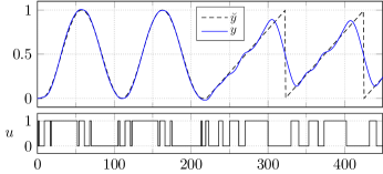
Note that Tables I and II give the required update rules for the NUV parameters of some generic scalar variable $X$, which are here applied to $X=U_{k}$ (with $\mathchoice{\overarrow@\arrowfill@\relbar\relbar\smallrightarrow\displaystyle{m}}{\overarrow@\arrowfill@\relbar\relbar\smallrightarrow\textstyle{m}}{\overarrow@\arrowfill@\relbar\relbar\smallrightarrow\scriptstyle{m}}{\overarrow@\arrowfill@\relbar\relbar\smallrightarrow\scriptscriptstyle{m}}_{\mspace{-3.0mu}X}=\mathchoice{\overarrow@\arrowfill@\relbar\relbar\smallrightarrow\displaystyle{m}}{\overarrow@\arrowfill@\relbar\relbar\smallrightarrow\textstyle{m}}{\overarrow@\arrowfill@\relbar\relbar\smallrightarrow\scriptstyle{m}}{\overarrow@\arrowfill@\relbar\relbar\smallrightarrow\scriptscriptstyle{m}}_{\mspace{-3.0mu}U_{k}}$ and $\mathchoice{\overarrow@\arrowfill@\relbar\relbar\smallrightarrow\displaystyle{V}}{\overarrow@\arrowfill@\relbar\relbar\smallrightarrow\textstyle{V}}{\overarrow@\arrowfill@\relbar\relbar\smallrightarrow\scriptstyle{V}}{\overarrow@\arrowfill@\relbar\relbar\smallrightarrow\scriptscriptstyle{V}}_{\mspace{-3.0mu}X}=\mathchoice{\overarrow@\arrowfill@\relbar\relbar\smallrightarrow\displaystyle{V}}{\overarrow@\arrowfill@\relbar\relbar\smallrightarrow\textstyle{V}}{\overarrow@\arrowfill@\relbar\relbar\smallrightarrow\scriptstyle{V}}{\overarrow@\arrowfill@\relbar\relbar\smallrightarrow\scriptscriptstyle{V}}_{\mspace{-3.0mu}U_{k}}$, respectively) and/or $X=Y_{k}$ (with $\mathchoice{\overarrow@\arrowfill@\relbar\relbar\smallrightarrow\displaystyle{m}}{\overarrow@\arrowfill@\relbar\relbar\smallrightarrow\textstyle{m}}{\overarrow@\arrowfill@\relbar\relbar\smallrightarrow\scriptstyle{m}}{\overarrow@\arrowfill@\relbar\relbar\smallrightarrow\scriptscriptstyle{m}}_{\mspace{-3.0mu}X}=\mathchoice{\overarrow@\arrowfill@\smallleftarrow\relbar\relbar\displaystyle{m}}{\overarrow@\arrowfill@\smallleftarrow\relbar\relbar\textstyle{m}}{\overarrow@\arrowfill@\smallleftarrow\relbar\relbar\scriptstyle{m}}{\overarrow@\arrowfill@\smallleftarrow\relbar\relbar\scriptscriptstyle{m}}_{\mspace{-3.0mu}Y_{k}}$ and $\mathchoice{\overarrow@\arrowfill@\relbar\relbar\smallrightarrow\displaystyle{V}}{\overarrow@\arrowfill@\relbar\relbar\smallrightarrow\textstyle{V}}{\overarrow@\arrowfill@\relbar\relbar\smallrightarrow\scriptstyle{V}}{\overarrow@\arrowfill@\relbar\relbar\smallrightarrow\scriptscriptstyle{V}}_{\mspace{-3.0mu}X}=\mathchoice{\overarrow@\arrowfill@\smallleftarrow\relbar\relbar\displaystyle{V}}{\overarrow@\arrowfill@\smallleftarrow\relbar\relbar\textstyle{V}}{\overarrow@\arrowfill@\smallleftarrow\relbar\relbar\scriptstyle{V}}{\overarrow@\arrowfill@\smallleftarrow\relbar\relbar\scriptscriptstyle{V}}_{\mspace{-3.0mu}Y_{k}}$, respectively), for $k\in\{1,\ldots,K\}$. More explanations will be given in Section IV. A preview of a first numerical example (a special case of Example II above) is shown in Fig. 2.

Figure 2: Binary-input control (or digital-to-analog conversion) as in Example II (cf. Section V-A), with target waveform $\breve{y}$ (dashed), binary control signal $u$ computed by the proposed algorithm (bottom), and resulting output signal y (solid blue).

The update rules in Table I are not new and stated here only for the sake of completeness. The derivations of the update rules in Table II will be given in Section III.

Prior	Use case	Update Rules
$\text{L}_{1}$ (Laplace) (see [5, 7])	sparsity	$\mathchoice{\overarrow@\arrowfill@\relbar\relbar\smallrightarrow\displaystyle{V}}{\overarrow@\arrowfill@\relbar\relbar\smallrightarrow\textstyle{V}}{\overarrow@\arrowfill@\relbar\relbar\smallrightarrow\scriptstyle{V}}{\overarrow@\arrowfill@\relbar\relbar\smallrightarrow\scriptscriptstyle{V}}_{\mspace{-3.0mu}X}=\gamma^{-1}|m_{X}|$
$\text{L}_{p}$ (see [5, 18])	various	$\displaystyle\mathchoice{\overarrow@\arrowfill@\relbar\relbar\smallrightarrow\displaystyle{V}}{\overarrow@\arrowfill@\relbar\relbar\smallrightarrow\textstyle{V}}{\overarrow@\arrowfill@\relbar\relbar\smallrightarrow\scriptstyle{V}}{\overarrow@\arrowfill@\relbar\relbar\smallrightarrow\scriptscriptstyle{V}}_{\mspace{-3.0mu}X}=\frac{|m_{X}|^{2-p}}{\gamma p}$
Smoothed $\text{L}_{1}$/Huber (see [7, 18])	outlier- insensitive fitting	$\displaystyle\mathchoice{\overarrow@\arrowfill@\relbar\relbar\smallrightarrow\displaystyle{V}}{\overarrow@\arrowfill@\relbar\relbar\smallrightarrow\textstyle{V}}{\overarrow@\arrowfill@\relbar\relbar\smallrightarrow\scriptstyle{V}}{\overarrow@\arrowfill@\relbar\relbar\smallrightarrow\scriptscriptstyle{V}}_{\mspace{-3.0mu}X}=\max\left\{r^{2},\frac{|m_{X}|}{\gamma}\right\}$
Plain NUV (see [8])	sparsity/jumps in a state space model	$\mathchoice{\overarrow@\arrowfill@\relbar\relbar\smallrightarrow\displaystyle{V}}{\overarrow@\arrowfill@\relbar\relbar\smallrightarrow\textstyle{V}}{\overarrow@\arrowfill@\relbar\relbar\smallrightarrow\scriptstyle{V}}{\overarrow@\arrowfill@\relbar\relbar\smallrightarrow\scriptscriptstyle{V}}_{\mspace{-3.0mu}X}=V_{X}+m_{X}^{2}$
Smoothed plain NUV (see [17, 18])	outlier- insensitive fitting	$\mathchoice{\overarrow@\arrowfill@\relbar\relbar\smallrightarrow\displaystyle{V}}{\overarrow@\arrowfill@\relbar\relbar\smallrightarrow\textstyle{V}}{\overarrow@\arrowfill@\relbar\relbar\smallrightarrow\scriptstyle{V}}{\overarrow@\arrowfill@\relbar\relbar\smallrightarrow\scriptscriptstyle{V}}_{\mspace{-3.0mu}X}=\max\left\{r^{2},m_{X}^{2}\right\}\quad$ or $\mathchoice{\overarrow@\arrowfill@\relbar\relbar\smallrightarrow\displaystyle{V}}{\overarrow@\arrowfill@\relbar\relbar\smallrightarrow\textstyle{V}}{\overarrow@\arrowfill@\relbar\relbar\smallrightarrow\scriptstyle{V}}{\overarrow@\arrowfill@\relbar\relbar\smallrightarrow\scriptscriptstyle{V}}_{\mspace{-3.0mu}X}=\max\left\{r^{2},V_{X}+m_{X}^{2}\right\}$

TABLE I: Update rules for the most useful basic NUV priors, with parameters $\gamma$ and $r^{2}$, cf. the cited references. (The mean $\mathchoice{\overarrow@\arrowfill@\relbar\relbar\smallrightarrow\displaystyle{m}}{\overarrow@\arrowfill@\relbar\relbar\smallrightarrow\textstyle{m}}{\overarrow@\arrowfill@\relbar\relbar\smallrightarrow\scriptstyle{m}}{\overarrow@\arrowfill@\relbar\relbar\smallrightarrow\scriptscriptstyle{m}}_{\mspace{-3.0mu}X}$ remains zero.)

Prior	Constraint	Update Rules
Half-space prior (Section III-B)	$x\geq a$	$\displaystyle\mathchoice{\overarrow@\arrowfill@\relbar\relbar\smallrightarrow\displaystyle{V}}{\overarrow@\arrowfill@\relbar\relbar\smallrightarrow\textstyle{V}}{\overarrow@\arrowfill@\relbar\relbar\smallrightarrow\scriptstyle{V}}{\overarrow@\arrowfill@\relbar\relbar\smallrightarrow\scriptscriptstyle{V}}_{\mspace{-3.0mu}X}=\frac{\left|m_{X}-a\right|}{\gamma}$ $\mathchoice{\overarrow@\arrowfill@\relbar\relbar\smallrightarrow\displaystyle{m}}{\overarrow@\arrowfill@\relbar\relbar\smallrightarrow\textstyle{m}}{\overarrow@\arrowfill@\relbar\relbar\smallrightarrow\scriptstyle{m}}{\overarrow@\arrowfill@\relbar\relbar\smallrightarrow\scriptscriptstyle{m}}_{\mspace{-3.0mu}X}=a+\left|m_{X}-a\right|$
	$x\leq a$	$\displaystyle\mathchoice{\overarrow@\arrowfill@\relbar\relbar\smallrightarrow\displaystyle{V}}{\overarrow@\arrowfill@\relbar\relbar\smallrightarrow\textstyle{V}}{\overarrow@\arrowfill@\relbar\relbar\smallrightarrow\scriptstyle{V}}{\overarrow@\arrowfill@\relbar\relbar\smallrightarrow\scriptscriptstyle{V}}_{\mspace{-3.0mu}X}=\frac{\left|m_{X}-a\right|}{\gamma}$ $\mathchoice{\overarrow@\arrowfill@\relbar\relbar\smallrightarrow\displaystyle{m}}{\overarrow@\arrowfill@\relbar\relbar\smallrightarrow\textstyle{m}}{\overarrow@\arrowfill@\relbar\relbar\smallrightarrow\scriptstyle{m}}{\overarrow@\arrowfill@\relbar\relbar\smallrightarrow\scriptscriptstyle{m}}_{\mspace{-3.0mu}X}=a-\left|m_{X}-a\right|$
Box prior (Section III-A)	$a\leq x\leq b$	$\displaystyle\mathchoice{\overarrow@\arrowfill@\relbar\relbar\smallrightarrow\displaystyle{V}}{\overarrow@\arrowfill@\relbar\relbar\smallrightarrow\textstyle{V}}{\overarrow@\arrowfill@\relbar\relbar\smallrightarrow\scriptstyle{V}}{\overarrow@\arrowfill@\relbar\relbar\smallrightarrow\scriptscriptstyle{V}}_{\mspace{-3.0mu}X}=\left(\frac{\gamma}{\left|m_{X}-a\right|}+\frac{\gamma}{\left|m_{X}-b\right|}\right)^{-1}$ $\displaystyle\mathchoice{\overarrow@\arrowfill@\relbar\relbar\smallrightarrow\displaystyle{m}}{\overarrow@\arrowfill@\relbar\relbar\smallrightarrow\textstyle{m}}{\overarrow@\arrowfill@\relbar\relbar\smallrightarrow\scriptstyle{m}}{\overarrow@\arrowfill@\relbar\relbar\smallrightarrow\scriptscriptstyle{m}}_{\mspace{-3.0mu}X}=\mathchoice{\overarrow@\arrowfill@\relbar\relbar\smallrightarrow\displaystyle{V}}{\overarrow@\arrowfill@\relbar\relbar\smallrightarrow\textstyle{V}}{\overarrow@\arrowfill@\relbar\relbar\smallrightarrow\scriptstyle{V}}{\overarrow@\arrowfill@\relbar\relbar\smallrightarrow\scriptscriptstyle{V}}_{\mspace{-3.0mu}X}\left(\frac{\gamma a}{\left|m_{X}-a\right|}+\frac{\gamma b}{\left|m_{X}-b\right|}\right)$
Binarizing prior ([19] and Section III-C)	$x\in\{a,b\}$	$\displaystyle\mathchoice{\overarrow@\arrowfill@\relbar\relbar\smallrightarrow\displaystyle{V}}{\overarrow@\arrowfill@\relbar\relbar\smallrightarrow\textstyle{V}}{\overarrow@\arrowfill@\relbar\relbar\smallrightarrow\scriptstyle{V}}{\overarrow@\arrowfill@\relbar\relbar\smallrightarrow\scriptscriptstyle{V}}_{\mspace{-3.0mu}X}=\left(\!\frac{1}{V_{X}\!+\!(m_{X}\!-\!a)^{2}}\!+\!\frac{1}{V_{X}\!+\!(m_{X}\!-\!b)^{2}}\!\right)^{\!-1}$ $\displaystyle\mathchoice{\overarrow@\arrowfill@\relbar\relbar\smallrightarrow\displaystyle{m}}{\overarrow@\arrowfill@\relbar\relbar\smallrightarrow\textstyle{m}}{\overarrow@\arrowfill@\relbar\relbar\smallrightarrow\scriptstyle{m}}{\overarrow@\arrowfill@\relbar\relbar\smallrightarrow\scriptscriptstyle{m}}_{\mspace{-3.0mu}X}=\mathchoice{\overarrow@\arrowfill@\relbar\relbar\smallrightarrow\displaystyle{V}}{\overarrow@\arrowfill@\relbar\relbar\smallrightarrow\textstyle{V}}{\overarrow@\arrowfill@\relbar\relbar\smallrightarrow\scriptstyle{V}}{\overarrow@\arrowfill@\relbar\relbar\smallrightarrow\scriptscriptstyle{V}}_{\mspace{-3.0mu}X}\!\left(\!\frac{a}{V_{X}\!+\!(m_{X}\!-\!a)^{2}}\!+\!\frac{b}{V_{X}\!+\!(m_{X}\!-\!b)^{2}}\!\right)$

TABLE II: Update rules for the composite NUV priors of Section III.

III Composite NUV Priors

In this section, we provide detailed derivations of the update rules stated in Table II.

We begin with a box prior, which constrains a model variable $x\in\mathbb{R}$ to be lower- and upper-bounded, i.e., $a\leq x\leq b$ with $a,b\in\mathbb{R}$. From the box prior, we derive a half-space prior, which constrains $x$ to be lower bounded or upper bounded, i.e., $x\geq a$ or $x\leq a$. Third, we describe a binarizing prior, which constrains $x$ to take values in a finite set with two elements, i.e, $x\in\{a,b\}$, with $a,b\in\mathbb{R}$. And finally, we discuss generalizations of the binarizing prior to $M>2$ levels.

In this section, we will describe and analyze these priors in a scalar setting; the sequence setting will be discussed in Section IV.

III-A Box Prior

III-A1 The Prior

The proposed NUV representation of the box constraint is obtained as an almost obvious combination of two ideas:

• The (well-known) NUV representation of the Laplace prior [5, 7].

• Adding two cost functions of the form $|x-a|$ and $|x-b|$ to create a cost function that is constant for $x\in[a,b]$, as illustrated in Fig. 3. (This idea is closely related to sum of absolute values (SOAV) optimization [33].)

Specifically, we will use the cost function

$$\kappa(x)\triangleq\gamma\big{(}|x-a|+|x-b|-|b-a|\big{)}$$ (8)

with sufficiently large $\gamma>0$ (as discussed in Section III-A2) and the associated prior

$$p(x)\triangleq\exp\!\big{(}-\kappa(x)\big{)}.$$ (9)

For the NUV representation, we first recall that the Laplace prior has the NUV representation

Figure 3: Cost function (8) (solid blue) for $a=-1,b=1$ and $\gamma=1$.

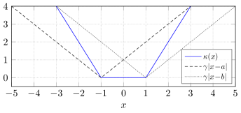
$$\exp\!\big{(}\!-\!\gamma|x|\big{)}=\max_{\sigma^{2}}\mathcal{N}\!\left({x;0,\sigma^{2}}\right)\tilde{\rho}(\sigma^{2}),$$ (10)

with $\gamma>0$ and with $\tilde{\rho}(\sigma^{2})\triangleq\sqrt{2\pi\sigma^{2}}e^{-\gamma^{2}\sigma^{2}/2}$ [7]. Furthermore, the maximizing variance in (10) is

$$\hat{\sigma}^{2}=\operatorname*{argmax}_{\sigma^{2}}\mathcal{N}\!\left({x;0,\sigma^{2}}\right)\tilde{\rho}(\sigma^{2})=\frac{|x|}{\gamma}.$$ (11)

The NUV representation of the prior (9) is then obtained as

$$p(x) = \exp\!\big{(}\!-\!\gamma|x-a|\big{)}\cdot\exp\!\big{(}\!-\!\gamma|x-b|\big{)}$$ (12)

$$= \max_{{\sigma_{a}^{2}}}\mathcal{N}\!\left({x;a,{\sigma_{a}^{2}}}\right)\tilde{\rho}({\sigma_{a}^{2}})\cdot\max_{{\sigma_{b}^{2}}}\mathcal{N}\!\left({x;b,{\sigma_{b}^{2}}}\right)\tilde{\rho}({\sigma_{b}^{2}}),$$ (13)

where we ignored the irrelevant constant term in (8). From (11), the maximizing variances in (13) are

$${{\hat{\sigma}_{a}}^{2}}=\frac{|x-a|}{\gamma}\quad\text{and}\quad{{\hat{\sigma}_{b}}^{2}}=\frac{|x-b|}{\gamma}.$$ (14)

We further note that (13) can be written as a (single) Gaussian probability density in $x$ and a scale factor that does not depend on $x$. Specifically, the prior can be written as

$$p(x) = \max_{\theta}p(x,\theta)=\max_{\theta}p(x\hskip 0.20004pt|\hskip 0.80002pt\theta)\rho(\theta)$$ (15)

with

$$p(x\hskip 0.20004pt|\hskip 0.80002pt\theta)=\mathcal{N}\!\left({x;{m_{\theta}},{\sigma_{\theta}^{2}}}\right)$$ (16)

and

$$\rho(\theta) = \mathcal{N}\!\left({a-b;0,{\sigma_{a}^{2}}+{\sigma_{b}^{2}}}\right)\tilde{\rho}({\sigma_{a}^{2}})\tilde{\rho}({\sigma_{b}^{2}}),$$ (17)

where $\theta\triangleq({\sigma_{a}^{2}},{\sigma_{b}^{2}})$,

$${\sigma_{\theta}^{2}}=\left(\frac{1}{{\sigma_{a}^{2}}}+\frac{1}{{\sigma_{b}^{2}}}\right)^{-1}\!\!\!\!,\;\;\text{and}\;\;{m_{\theta}}={\sigma_{\theta}^{2}}\left(\frac{a}{{\sigma_{a}^{2}}}+\frac{b}{{\sigma_{b}^{2}}}\right).$$ (18)

Note that $p(x,\theta)$ in (15) can be seen as a (improper) joint prior on $X$ and $\theta$. The derivation of (16)–(18) follows from standard properties of Gaussian probability densities, cf. [34, Section 1]. (The factor (17) will actually not be used below.)

Finally, plugging the maximizing variances (14) into (18) yields the closed-form update rules

$$\mathchoice{\overarrow@\arrowfill@\relbar\relbar\smallrightarrow\displaystyle{V}}{\overarrow@\arrowfill@\relbar\relbar\smallrightarrow\textstyle{V}}{\overarrow@\arrowfill@\relbar\relbar\smallrightarrow\scriptstyle{V}}{\overarrow@\arrowfill@\relbar\relbar\smallrightarrow\scriptscriptstyle{V}}_{\mspace{-3.0mu}X} = \left(\frac{\gamma}{\left|x-a\right|}+\frac{\gamma}{\left|x-b\right|}\right)^{-1}$$ (19)

$$\mathchoice{\overarrow@\arrowfill@\relbar\relbar\smallrightarrow\displaystyle{m}}{\overarrow@\arrowfill@\relbar\relbar\smallrightarrow\textstyle{m}}{\overarrow@\arrowfill@\relbar\relbar\smallrightarrow\scriptstyle{m}}{\overarrow@\arrowfill@\relbar\relbar\smallrightarrow\scriptscriptstyle{m}}_{\mspace{-3.0mu}X} = \mathchoice{\overarrow@\arrowfill@\relbar\relbar\smallrightarrow\displaystyle{V}}{\overarrow@\arrowfill@\relbar\relbar\smallrightarrow\textstyle{V}}{\overarrow@\arrowfill@\relbar\relbar\smallrightarrow\scriptstyle{V}}{\overarrow@\arrowfill@\relbar\relbar\smallrightarrow\scriptscriptstyle{V}}_{\mspace{-3.0mu}X}\left(\frac{\gamma a}{\left|x-a\right|}+\frac{\gamma b}{\left|x-b\right|}\right),$$ (20)

which are given in Table II (in slightly different notation). In summary, the NUV representation of the box constraint amounts to a Gaussian prior (up to a scale factor) with mean and variance given by (20) and (19), respectively.

III-A2 Analysis of the Scalar Case

In order to study the constraining effect of the proposed prior, we now assume that the joint prior $p(x,\theta)$ in (15) is used in some model with fixed observation(s) $\breve{y}$ and likelihood function $p(\breve{y}\hskip 0.20004pt|\hskip 0.80002ptx)$. Moreover, we assume $p(\breve{y}\hskip 0.20004pt|\hskip 0.80002ptx)$ to be Gaussian in $x$, with mean $\mu$ and variance $s^{2}$ depending on $\breve{y}$, i.e.,

$$p(\breve{y}\hskip 0.20004pt|\hskip 0.80002ptx)\triangleq\mathcal{N}\!\left({x;\mu,s^{2}}\right).$$ (21)

The resulting statistical model is

$$p(\breve{y}\hskip 0.20004pt|\hskip 0.80002ptx)p(x,\theta) = \mathcal{N}\!\left({x;\mu,s^{2}}\right)\cdot\mathcal{N}\!\left({x;a,{\sigma_{a}^{2}}}\right)\tilde{\rho}(\sigma_{a})$$ (22)

$$\cdot\mathcal{N}\!\left({x;b,{\sigma_{b}^{2}}}\right)\tilde{\rho}(\sigma_{b}),$$

which is illustrated as factor graph [35] in Fig. 4.

Figure 4: Factor graph representation of statistical model (22). The boxes labeled $\mathcal{N}\!\left({0,\sigma^{2}}\right)$ represent zero-mean normal probability density functions.

Assume now that $x$ and $\theta$ are determined by joint MAP estimation according to

$$\hat{x} = \operatorname*{argmax}_{x}\max_{\theta}p(\breve{y}\hskip 0.20004pt|\hskip 0.80002ptx)p(x,\theta),$$ (23)

with $p(x,\theta)$ as in (15). In the scalar setting of this section, the estimate (23) can certainly be computed numerically, but such a brute-force approach does not generalize to the sequence setting of Section IV. With that generalization in mind, we consider computing (23) by alternating maximization (AM) over $x$ and $\theta$. As mentioned, the maximization over $\theta$ in (23) can be carried out explicitly, and (23) can be solved by iteratively maximizing

$$\hat{x} = \operatorname*{argmax}_{x}p(\breve{y}\hskip 0.20004pt|\hskip 0.80002ptx)\mathcal{N}\!\left({x;\mathchoice{\overarrow@\arrowfill@\relbar\relbar\smallrightarrow\displaystyle{m}}{\overarrow@\arrowfill@\relbar\relbar\smallrightarrow\textstyle{m}}{\overarrow@\arrowfill@\relbar\relbar\smallrightarrow\scriptstyle{m}}{\overarrow@\arrowfill@\relbar\relbar\smallrightarrow\scriptscriptstyle{m}}_{\mspace{-3.0mu}X},\mathchoice{\overarrow@\arrowfill@\relbar\relbar\smallrightarrow\displaystyle{V}}{\overarrow@\arrowfill@\relbar\relbar\smallrightarrow\textstyle{V}}{\overarrow@\arrowfill@\relbar\relbar\smallrightarrow\scriptstyle{V}}{\overarrow@\arrowfill@\relbar\relbar\smallrightarrow\scriptscriptstyle{V}}_{\mspace{-3.0mu}X}}\right),$$ (24)

and updating $\mathchoice{\overarrow@\arrowfill@\relbar\relbar\smallrightarrow\displaystyle{m}}{\overarrow@\arrowfill@\relbar\relbar\smallrightarrow\textstyle{m}}{\overarrow@\arrowfill@\relbar\relbar\smallrightarrow\scriptstyle{m}}{\overarrow@\arrowfill@\relbar\relbar\smallrightarrow\scriptscriptstyle{m}}_{\mspace{-3.0mu}X}$ and $\mathchoice{\overarrow@\arrowfill@\relbar\relbar\smallrightarrow\displaystyle{V}}{\overarrow@\arrowfill@\relbar\relbar\smallrightarrow\textstyle{V}}{\overarrow@\arrowfill@\relbar\relbar\smallrightarrow\scriptstyle{V}}{\overarrow@\arrowfill@\relbar\relbar\smallrightarrow\scriptscriptstyle{V}}_{\mspace{-3.0mu}X}$ according to (20) and (19). More specifically, we alternate the following two steps in iterations $i=1,2,3,\ldots$:

1. For fixed $\mathchoice{\overarrow@\arrowfill@\relbar\relbar\smallrightarrow\displaystyle{m}}{\overarrow@\arrowfill@\relbar\relbar\smallrightarrow\textstyle{m}}{\overarrow@\arrowfill@\relbar\relbar\smallrightarrow\scriptstyle{m}}{\overarrow@\arrowfill@\relbar\relbar\smallrightarrow\scriptscriptstyle{m}}_{\mspace{-3.0mu}X}^{(i-1)}$ and $\mathchoice{\overarrow@\arrowfill@\relbar\relbar\smallrightarrow\displaystyle{V}}{\overarrow@\arrowfill@\relbar\relbar\smallrightarrow\textstyle{V}}{\overarrow@\arrowfill@\relbar\relbar\smallrightarrow\scriptstyle{V}}{\overarrow@\arrowfill@\relbar\relbar\smallrightarrow\scriptscriptstyle{V}}_{\mspace{-3.0mu}X}^{(i-1)}$, compute the MAP estimate

   $$\hat{x}^{(i)} = \operatorname*{argmax}_{x}p(\breve{y}\hskip 0.20004pt|\hskip 0.80002ptx)\mathcal{N}\!\left({x;\mathchoice{\overarrow@\arrowfill@\relbar\relbar\smallrightarrow\displaystyle{m}}{\overarrow@\arrowfill@\relbar\relbar\smallrightarrow\textstyle{m}}{\overarrow@\arrowfill@\relbar\relbar\smallrightarrow\scriptstyle{m}}{\overarrow@\arrowfill@\relbar\relbar\smallrightarrow\scriptscriptstyle{m}}_{\mspace{-3.0mu}X}^{(i-1)},\mathchoice{\overarrow@\arrowfill@\relbar\relbar\smallrightarrow\displaystyle{V}}{\overarrow@\arrowfill@\relbar\relbar\smallrightarrow\textstyle{V}}{\overarrow@\arrowfill@\relbar\relbar\smallrightarrow\scriptstyle{V}}{\overarrow@\arrowfill@\relbar\relbar\smallrightarrow\scriptscriptstyle{V}}_{\mspace{-3.0mu}X}^{(i-1)}}\right)$$ (25)

   $$= \left(\frac{1}{\mathchoice{\overarrow@\arrowfill@\relbar\relbar\smallrightarrow\displaystyle{V}}{\overarrow@\arrowfill@\relbar\relbar\smallrightarrow\textstyle{V}}{\overarrow@\arrowfill@\relbar\relbar\smallrightarrow\scriptstyle{V}}{\overarrow@\arrowfill@\relbar\relbar\smallrightarrow\scriptscriptstyle{V}}_{\mspace{-3.0mu}X}^{(i-1)}}+\frac{1}{s^{2}}\right)^{-1}\!\!\left(\frac{\mathchoice{\overarrow@\arrowfill@\relbar\relbar\smallrightarrow\displaystyle{m}}{\overarrow@\arrowfill@\relbar\relbar\smallrightarrow\textstyle{m}}{\overarrow@\arrowfill@\relbar\relbar\smallrightarrow\scriptstyle{m}}{\overarrow@\arrowfill@\relbar\relbar\smallrightarrow\scriptscriptstyle{m}}_{\mspace{-3.0mu}X}^{(i-1)}}{\mathchoice{\overarrow@\arrowfill@\relbar\relbar\smallrightarrow\displaystyle{V}}{\overarrow@\arrowfill@\relbar\relbar\smallrightarrow\textstyle{V}}{\overarrow@\arrowfill@\relbar\relbar\smallrightarrow\scriptstyle{V}}{\overarrow@\arrowfill@\relbar\relbar\smallrightarrow\scriptscriptstyle{V}}_{\mspace{-3.0mu}X}^{(i-1)}}+\frac{\mu}{s^{2}}\right)\!.$$ (26)

2. For fixed $x=\hat{x}^{(i)}$, compute $\mathchoice{\overarrow@\arrowfill@\relbar\relbar\smallrightarrow\displaystyle{m}}{\overarrow@\arrowfill@\relbar\relbar\smallrightarrow\textstyle{m}}{\overarrow@\arrowfill@\relbar\relbar\smallrightarrow\scriptstyle{m}}{\overarrow@\arrowfill@\relbar\relbar\smallrightarrow\scriptscriptstyle{m}}_{\mspace{-3.0mu}X}^{(i)}$ and $\mathchoice{\overarrow@\arrowfill@\relbar\relbar\smallrightarrow\displaystyle{V}}{\overarrow@\arrowfill@\relbar\relbar\smallrightarrow\textstyle{V}}{\overarrow@\arrowfill@\relbar\relbar\smallrightarrow\scriptstyle{V}}{\overarrow@\arrowfill@\relbar\relbar\smallrightarrow\scriptscriptstyle{V}}_{\mspace{-3.0mu}X}^{(i)}$ according to (20) and (19), respectively.

Note that this AM is guaranteed to converge to a local maximum or a saddle point, provided that the underlying objective function is smooth; in the present case, the estimate (25) is thus guaranteed to converge to (23).

Some numerical results with the estimate (23) are shown in Fig. 5.

Figure 5: Estimate (23) for $a=-1$, $b=1$, $\gamma=1$, and different values of $s^{2}$. The unknown parameters were initialized to $\mathchoice{\overarrow@\arrowfill@\relbar\relbar\smallrightarrow\displaystyle{m}}{\overarrow@\arrowfill@\relbar\relbar\smallrightarrow\textstyle{m}}{\overarrow@\arrowfill@\relbar\relbar\smallrightarrow\scriptstyle{m}}{\overarrow@\arrowfill@\relbar\relbar\smallrightarrow\scriptscriptstyle{m}}_{\mspace{-3.0mu}X}^{(0)}=0$ and $\mathchoice{\overarrow@\arrowfill@\relbar\relbar\smallrightarrow\displaystyle{V}}{\overarrow@\arrowfill@\relbar\relbar\smallrightarrow\textstyle{V}}{\overarrow@\arrowfill@\relbar\relbar\smallrightarrow\scriptstyle{V}}{\overarrow@\arrowfill@\relbar\relbar\smallrightarrow\scriptscriptstyle{V}}_{\mspace{-3.0mu}X}^{(0)}=1$.

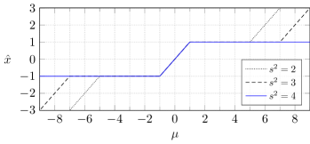
We observe that for given $\mu$ and $\gamma>0$, and sufficiently large $s^{2}$, the estimate (23) is indeed restricted to $a\leq\hat{x}\leq b$. Quantitatively, we have

• Theorem 1. The estimate (23) satisfies $a\leq\hat{x}\leq b$ if and only if

  $$s^{2}>\begin{cases}0&\text{if $a\leq\mu\leq b$},\\ \min\left\{\frac{|a-\mu|}{2\gamma},\frac{|b-\mu|}{2\gamma}\right\}&\text{otherwise}.\end{cases}$$ (27)

  $\Box$

Since $\gamma$ is a free design parameter, it can essentially always be chosen so that $a\leq\hat{x}\leq b$. The proof of Theorem III-A2 is given in Appendix A-A.

III-B Half-Space Prior

III-B1 The Prior

Taking the limit $b\rightarrow\infty$ in (8) yields

$$\kappa(x) = \begin{cases}2\gamma(a-x)&\text{if $x<a$},\\ 0&\text{otherwise},\end{cases}$$ (28)

and taking the limit $b\rightarrow-\infty$ in (8) yields

$$\kappa(x) = \begin{cases}0&\text{if $x<a$},\\ 2\gamma(x-a)&\text{otherwise}.\end{cases}$$ (29)

The cost function (28) is shown in Fig. 6.

By taking the limit $b\rightarrow\infty$ in (19) and (20), we further obtain

$$\mathchoice{\overarrow@\arrowfill@\relbar\relbar\smallrightarrow\displaystyle{V}}{\overarrow@\arrowfill@\relbar\relbar\smallrightarrow\textstyle{V}}{\overarrow@\arrowfill@\relbar\relbar\smallrightarrow\scriptstyle{V}}{\overarrow@\arrowfill@\relbar\relbar\smallrightarrow\scriptscriptstyle{V}}_{\mspace{-3.0mu}X} = \lim_{{b\rightarrow\infty}}\left(\frac{\gamma}{\left|x-a\right|}+\frac{\gamma}{\left|x-b\right|}\right)^{-1}=\frac{|x-a|}{\gamma}$$ (30)

$$\mathchoice{\overarrow@\arrowfill@\relbar\relbar\smallrightarrow\displaystyle{m}}{\overarrow@\arrowfill@\relbar\relbar\smallrightarrow\textstyle{m}}{\overarrow@\arrowfill@\relbar\relbar\smallrightarrow\scriptstyle{m}}{\overarrow@\arrowfill@\relbar\relbar\smallrightarrow\scriptscriptstyle{m}}_{\mspace{-3.0mu}X} = \lim_{{b\rightarrow\infty}}\mathchoice{\overarrow@\arrowfill@\relbar\relbar\smallrightarrow\displaystyle{V}}{\overarrow@\arrowfill@\relbar\relbar\smallrightarrow\textstyle{V}}{\overarrow@\arrowfill@\relbar\relbar\smallrightarrow\scriptstyle{V}}{\overarrow@\arrowfill@\relbar\relbar\smallrightarrow\scriptscriptstyle{V}}_{\mspace{-3.0mu}X}\left(\frac{\gamma a}{\left|x-a\right|}+\frac{\gamma b}{\left|x-b\right|}\right)=a+|x-a|$$ (31)

for the right-sided half-space prior, and by taking the limit $b\rightarrow-\infty$ in (19) and (20), we obtain

$$\mathchoice{\overarrow@\arrowfill@\relbar\relbar\smallrightarrow\displaystyle{V}}{\overarrow@\arrowfill@\relbar\relbar\smallrightarrow\textstyle{V}}{\overarrow@\arrowfill@\relbar\relbar\smallrightarrow\scriptstyle{V}}{\overarrow@\arrowfill@\relbar\relbar\smallrightarrow\scriptscriptstyle{V}}_{\mspace{-3.0mu}X} = \frac{|x-a|}{\gamma}$$ (32)

$$\mathchoice{\overarrow@\arrowfill@\relbar\relbar\smallrightarrow\displaystyle{m}}{\overarrow@\arrowfill@\relbar\relbar\smallrightarrow\textstyle{m}}{\overarrow@\arrowfill@\relbar\relbar\smallrightarrow\scriptstyle{m}}{\overarrow@\arrowfill@\relbar\relbar\smallrightarrow\scriptscriptstyle{m}}_{\mspace{-3.0mu}X} = a-|x-a|$$ (33)

for the left-sided half-space prior, which are the update rules in Table II (in slightly different notation).

Figure 6: Cost function (28) of a ride-sided half-space prior, for $a=0$ and different values of $\gamma$.

III-B2 Analysis of the Scalar Case

We proceed to examine the proposed prior in a model as in Section III-A2, with $p(\breve{y}\hskip 0.20004pt|\hskip 0.80002ptx)$ as in (21). Analogously, we compute the estimate

$$\hat{x} = \operatorname*{argmax}_{x}p(\breve{y}\hskip 0.20004pt|\hskip 0.80002ptx)\mathcal{N}\!\left({x;\mathchoice{\overarrow@\arrowfill@\relbar\relbar\smallrightarrow\displaystyle{m}}{\overarrow@\arrowfill@\relbar\relbar\smallrightarrow\textstyle{m}}{\overarrow@\arrowfill@\relbar\relbar\smallrightarrow\scriptstyle{m}}{\overarrow@\arrowfill@\relbar\relbar\smallrightarrow\scriptscriptstyle{m}}_{\mspace{-3.0mu}X},\mathchoice{\overarrow@\arrowfill@\relbar\relbar\smallrightarrow\displaystyle{V}}{\overarrow@\arrowfill@\relbar\relbar\smallrightarrow\textstyle{V}}{\overarrow@\arrowfill@\relbar\relbar\smallrightarrow\scriptstyle{V}}{\overarrow@\arrowfill@\relbar\relbar\smallrightarrow\scriptscriptstyle{V}}_{\mspace{-3.0mu}X}}\right)$$ (34)

by iterating the two steps outlined in Section III-A2, except that $\mathchoice{\overarrow@\arrowfill@\relbar\relbar\smallrightarrow\displaystyle{m}}{\overarrow@\arrowfill@\relbar\relbar\smallrightarrow\textstyle{m}}{\overarrow@\arrowfill@\relbar\relbar\smallrightarrow\scriptstyle{m}}{\overarrow@\arrowfill@\relbar\relbar\smallrightarrow\scriptscriptstyle{m}}_{\mspace{-3.0mu}X}$ and $\mathchoice{\overarrow@\arrowfill@\relbar\relbar\smallrightarrow\displaystyle{V}}{\overarrow@\arrowfill@\relbar\relbar\smallrightarrow\textstyle{V}}{\overarrow@\arrowfill@\relbar\relbar\smallrightarrow\scriptstyle{V}}{\overarrow@\arrowfill@\relbar\relbar\smallrightarrow\scriptscriptstyle{V}}_{\mspace{-3.0mu}X}$ are updated according to (31) and (30), or (33) and (32), respectively. More specifically, we alternate the following two steps in iterations $i=1,2,3,\ldots$:

1. For fixed $\mathchoice{\overarrow@\arrowfill@\relbar\relbar\smallrightarrow\displaystyle{m}}{\overarrow@\arrowfill@\relbar\relbar\smallrightarrow\textstyle{m}}{\overarrow@\arrowfill@\relbar\relbar\smallrightarrow\scriptstyle{m}}{\overarrow@\arrowfill@\relbar\relbar\smallrightarrow\scriptscriptstyle{m}}_{\mspace{-3.0mu}X}^{(i-1)}$ and $\mathchoice{\overarrow@\arrowfill@\relbar\relbar\smallrightarrow\displaystyle{V}}{\overarrow@\arrowfill@\relbar\relbar\smallrightarrow\textstyle{V}}{\overarrow@\arrowfill@\relbar\relbar\smallrightarrow\scriptstyle{V}}{\overarrow@\arrowfill@\relbar\relbar\smallrightarrow\scriptscriptstyle{V}}_{\mspace{-3.0mu}X}^{(i-1)}$, compute the MAP estimate

   $$\hat{x}^{(i)} = \operatorname*{argmax}_{x}p(\breve{y}\hskip 0.20004pt|\hskip 0.80002ptx)\mathcal{N}\!\left({x;\mathchoice{\overarrow@\arrowfill@\relbar\relbar\smallrightarrow\displaystyle{m}}{\overarrow@\arrowfill@\relbar\relbar\smallrightarrow\textstyle{m}}{\overarrow@\arrowfill@\relbar\relbar\smallrightarrow\scriptstyle{m}}{\overarrow@\arrowfill@\relbar\relbar\smallrightarrow\scriptscriptstyle{m}}_{\mspace{-3.0mu}X}^{(i-1)},\mathchoice{\overarrow@\arrowfill@\relbar\relbar\smallrightarrow\displaystyle{V}}{\overarrow@\arrowfill@\relbar\relbar\smallrightarrow\textstyle{V}}{\overarrow@\arrowfill@\relbar\relbar\smallrightarrow\scriptstyle{V}}{\overarrow@\arrowfill@\relbar\relbar\smallrightarrow\scriptscriptstyle{V}}_{\mspace{-3.0mu}X}^{(i-1)}}\right)$$ (35)

   $$= \left(\frac{1}{\mathchoice{\overarrow@\arrowfill@\relbar\relbar\smallrightarrow\displaystyle{V}}{\overarrow@\arrowfill@\relbar\relbar\smallrightarrow\textstyle{V}}{\overarrow@\arrowfill@\relbar\relbar\smallrightarrow\scriptstyle{V}}{\overarrow@\arrowfill@\relbar\relbar\smallrightarrow\scriptscriptstyle{V}}_{\mspace{-3.0mu}X}^{(i-1)}}+\frac{1}{s^{2}}\right)^{-1}\!\!\left(\frac{\mathchoice{\overarrow@\arrowfill@\relbar\relbar\smallrightarrow\displaystyle{m}}{\overarrow@\arrowfill@\relbar\relbar\smallrightarrow\textstyle{m}}{\overarrow@\arrowfill@\relbar\relbar\smallrightarrow\scriptstyle{m}}{\overarrow@\arrowfill@\relbar\relbar\smallrightarrow\scriptscriptstyle{m}}_{\mspace{-3.0mu}X}^{(i-1)}}{\mathchoice{\overarrow@\arrowfill@\relbar\relbar\smallrightarrow\displaystyle{V}}{\overarrow@\arrowfill@\relbar\relbar\smallrightarrow\textstyle{V}}{\overarrow@\arrowfill@\relbar\relbar\smallrightarrow\scriptstyle{V}}{\overarrow@\arrowfill@\relbar\relbar\smallrightarrow\scriptscriptstyle{V}}_{\mspace{-3.0mu}X}^{(i-1)}}+\frac{\mu}{s^{2}}\right)\!.$$ (36)

2. For fixed $x=\hat{x}^{(i)}$, compute $\mathchoice{\overarrow@\arrowfill@\relbar\relbar\smallrightarrow\displaystyle{m}}{\overarrow@\arrowfill@\relbar\relbar\smallrightarrow\textstyle{m}}{\overarrow@\arrowfill@\relbar\relbar\smallrightarrow\scriptstyle{m}}{\overarrow@\arrowfill@\relbar\relbar\smallrightarrow\scriptscriptstyle{m}}_{\mspace{-3.0mu}X}^{(i)}$ and $\mathchoice{\overarrow@\arrowfill@\relbar\relbar\smallrightarrow\displaystyle{V}}{\overarrow@\arrowfill@\relbar\relbar\smallrightarrow\textstyle{V}}{\overarrow@\arrowfill@\relbar\relbar\smallrightarrow\scriptstyle{V}}{\overarrow@\arrowfill@\relbar\relbar\smallrightarrow\scriptscriptstyle{V}}_{\mspace{-3.0mu}X}^{(i)}$ according to (31) and (30), or (33) and (32), respectively.

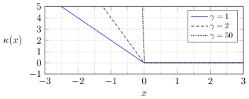
Some numerical results of the estimate (34) are shown in Fig. 7.

Figure 7: Estimate (34) for $a=0$, ${b\rightarrow\infty}$, $\gamma=1$, and different values for $s^{2}$. The unknown parameters were initialized to $\mathchoice{\overarrow@\arrowfill@\relbar\relbar\smallrightarrow\displaystyle{m}}{\overarrow@\arrowfill@\relbar\relbar\smallrightarrow\textstyle{m}}{\overarrow@\arrowfill@\relbar\relbar\smallrightarrow\scriptstyle{m}}{\overarrow@\arrowfill@\relbar\relbar\smallrightarrow\scriptscriptstyle{m}}_{\mspace{-3.0mu}X}^{(0)}=0$ and $\mathchoice{\overarrow@\arrowfill@\relbar\relbar\smallrightarrow\displaystyle{V}}{\overarrow@\arrowfill@\relbar\relbar\smallrightarrow\textstyle{V}}{\overarrow@\arrowfill@\relbar\relbar\smallrightarrow\scriptstyle{V}}{\overarrow@\arrowfill@\relbar\relbar\smallrightarrow\scriptscriptstyle{V}}_{\mspace{-3.0mu}X}^{(0)}=1$.

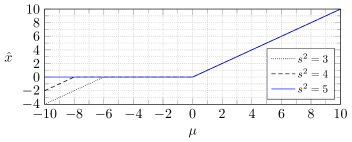
We observe that for any fixed $\mu$ and $\gamma$, and sufficiently large $s^{2}$, the estimate (34) indeed satisfies $\hat{x}\geq a$. Quantitatively, we have

• Theorem 2. For a right-sided constraint, the estimate (34) satisfies $\hat{x}\geq a$ if and only if

  $$s^{2}>\begin{cases}0&\text{if $\mu\geq a$},\\ \frac{|a-\mu|}{2\gamma}&\mathrm{otherwise}.\end{cases}$$ (37)

  Analogously, for a left-sided constraint, $\hat{x}\leq a$ if and only if

  $$s^{2}>\begin{cases}0&\text{if $\mu\leq a$},\\ \frac{|a-\mu|}{2\gamma}&\mathrm{otherwise}.\end{cases}$$ (38)

  $\Box$

Note that since $\gamma$ is a free design parameter, (37) (or (38), respectively) can essentially always be satisfied. The proof of Theorem III-B2 is easily obtained as a suitably simplified version of the proof of Theorem III-A2.

III-C Binarizing Prior

In this section, we discuss the composite NUV representation of a binarizing constraint (enforcing $x\in\{a,b\}$) that was proposed in [19].

III-C1 The Prior

Consider

$$p(x,\theta)\triangleq\mathcal{N}\!\left({x;a,{\sigma_{a}^{2}}}\right)\mathcal{N}\!\left({x;b,{\sigma_{b}^{2}}}\right),$$ (39)

where $\theta\triangleq({\sigma_{a}^{2}},{\sigma_{b}^{2}})$ is a shorthand for the two variances in (39). It turns out that this prior strongly prefers $X$ to lie in $\{a,b\}$. The detailed working of this binarizing effect depends on how the unknown variances $\theta$ are determined. Two different ways to estimate these variances are considered in Sections III-C4 and III-C5.

Before examining this binarizing effect, we first note that, for fixed variances $\theta$, $p(x,\theta)$ is a Gaussian probability density in $x$ (up to a scale factor). Specifically, $p(x,\theta)$ can be written as

$$p(x,\theta)=p(x\hskip 0.20004pt|\hskip 0.80002pt\theta)\rho(\theta)$$ (40)

with

$$p(x\hskip 0.20004pt|\hskip 0.80002pt\theta)=\mathcal{N}\!\left({x;{m_{\theta}},{\sigma_{\theta}^{2}}}\right),$$ (41)

and ${m_{\theta}}$ and ${\sigma_{\theta}^{2}}$ as in (18), and with

$$\rho(\theta)=\mathcal{N}\!\left({a-b;0,{\sigma_{a}^{2}}+{\sigma_{b}^{2}}}\right).$$ (42)

III-C2 Cost Function for MAP Estimation

Assume for now that the unknown variances $\theta$ are determined by

$$\hat{\theta}=\operatorname*{argmax}_{\theta}p(x,\theta).$$ (43)

(However, we will see that estimating $\theta$ as in Section III-C5 works much better.) We then obtain

$$\hat{\theta}=({{\hat{\sigma}_{a}}^{2}},{{\hat{\sigma}_{b}}^{2}})=\left((x-a)^{2},(x-b)^{2}\right),$$ (44)

cf. Appendix A-B. The effective prior is then obtained by plugging (44) into (39), resulting in

$$p(x)\triangleq p(x,\hat{\theta})\propto\frac{1}{|x-a|\cdot|x-b|}$$ (45)

with associated cost function

$$\kappa(x)=-\log p(x)=\log|x-a|+\log|x-b|+\operatorname{const.}$$ (46)

The cost function (46) is illustrated in Fig. 8. It is obvious that such a prior strongly favors $X$ to lie in $\{a,b\}$.

Figure 8: The cost function (46) for $a=0$ and $b=1$.

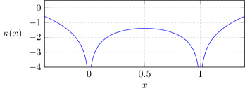
III-C3 Analysis of the Scalar Case

In order to further study the binarizing effect of the proposed prior, we now assume that (39) is used in a model as in Section III-A2, with $p(\breve{y}\hskip 0.20004pt|\hskip 0.80002ptx)$ as in (21). A factor graph of the resulting statistical model

$$p(\breve{y}\hskip 0.20004pt|\hskip 0.80002ptx)p(x,\theta)=\mathcal{N}\!\left({x;\mu,s^{2}}\right)\mathcal{N}\!\left({x;a,{\sigma_{a}^{2}}}\right)\mathcal{N}\!\left({x;b,{\sigma_{b}^{2}}}\right)$$ (47)

is shown in Fig. 9.

Figure 9: Factor graph of (47) for fixed $\breve{y}$, with parameters $\mu$ and $s^{2}$ depending on $\breve{y}$.

As mentioned, the detailed working of the binarizing effect of $p(x,\theta)$ depends on how the unknown variances $\theta$ are determined. Two different ways to estimate these variances are considered in Sections III-C4 and III-C5. Empirically, the method of Section III-C5 works much better than the method of Section III-C4, which confirms what has long been known for other NUV priors [36].

III-C4 Joint MAP Estimation

An obvious approach to estimate $x$ and $\theta$ is by joint MAP estimation, which results in

$$\hat{x} = \operatorname*{argmax}_{x}\max_{\theta}p(\breve{y}\hskip 0.20004pt|\hskip 0.80002ptx)p(x,\theta)$$ (48)

$$= \operatorname*{argmax}_{x}p(\breve{y}\hskip 0.20004pt|\hskip 0.80002ptx)p(x)$$ (49)

$$= \operatorname*{argmax}_{x}\frac{\mathcal{N}\!\left({x;\mu,s^{2}}\right)}{|x-a|\cdot|x-b|}.$$ (50)

In the scalar setting of this section, the estimate (48) can certainly be computed numerically for any $s^{2}$, but such a brute-force approach does not generalize to the sequence setting of Section IV. With that generalization in mind, we now consider computing (48) by AM over $x$ and $\theta$. As in Section III-A1, we precompute the maximization over $\theta$ by plugging the maximizing variances (44) into (18), resulting in the closed-form update rules

$$\mathchoice{\overarrow@\arrowfill@\relbar\relbar\smallrightarrow\displaystyle{V}}{\overarrow@\arrowfill@\relbar\relbar\smallrightarrow\textstyle{V}}{\overarrow@\arrowfill@\relbar\relbar\smallrightarrow\scriptstyle{V}}{\overarrow@\arrowfill@\relbar\relbar\smallrightarrow\scriptscriptstyle{V}}_{\mspace{-3.0mu}X} = \left(\frac{1}{(x-a)^{2}}+\frac{1}{(x-b)^{2}}\right)^{-1}$$ (51)

$$\mathchoice{\overarrow@\arrowfill@\relbar\relbar\smallrightarrow\displaystyle{m}}{\overarrow@\arrowfill@\relbar\relbar\smallrightarrow\textstyle{m}}{\overarrow@\arrowfill@\relbar\relbar\smallrightarrow\scriptstyle{m}}{\overarrow@\arrowfill@\relbar\relbar\smallrightarrow\scriptscriptstyle{m}}_{\mspace{-3.0mu}X} = \mathchoice{\overarrow@\arrowfill@\relbar\relbar\smallrightarrow\displaystyle{V}}{\overarrow@\arrowfill@\relbar\relbar\smallrightarrow\textstyle{V}}{\overarrow@\arrowfill@\relbar\relbar\smallrightarrow\scriptstyle{V}}{\overarrow@\arrowfill@\relbar\relbar\smallrightarrow\scriptscriptstyle{V}}_{\mspace{-3.0mu}X}\left(\frac{a}{(x-a)^{2}}+\frac{b}{(x-b)^{2}}\right).$$ (52)

Consequently, computing (48) by AM amounts to computing

$$\hat{x} = \operatorname*{argmax}_{x}p(\breve{y}\hskip 0.20004pt|\hskip 0.80002ptx)\mathcal{N}\!\left({x;\mathchoice{\overarrow@\arrowfill@\relbar\relbar\smallrightarrow\displaystyle{m}}{\overarrow@\arrowfill@\relbar\relbar\smallrightarrow\textstyle{m}}{\overarrow@\arrowfill@\relbar\relbar\smallrightarrow\scriptstyle{m}}{\overarrow@\arrowfill@\relbar\relbar\smallrightarrow\scriptscriptstyle{m}}_{\mspace{-3.0mu}X},\mathchoice{\overarrow@\arrowfill@\relbar\relbar\smallrightarrow\displaystyle{V}}{\overarrow@\arrowfill@\relbar\relbar\smallrightarrow\textstyle{V}}{\overarrow@\arrowfill@\relbar\relbar\smallrightarrow\scriptstyle{V}}{\overarrow@\arrowfill@\relbar\relbar\smallrightarrow\scriptscriptstyle{V}}_{\mspace{-3.0mu}X}}\right)$$ (53)

by iterating the two steps outlined in Section III-A2, except that $\mathchoice{\overarrow@\arrowfill@\relbar\relbar\smallrightarrow\displaystyle{m}}{\overarrow@\arrowfill@\relbar\relbar\smallrightarrow\textstyle{m}}{\overarrow@\arrowfill@\relbar\relbar\smallrightarrow\scriptstyle{m}}{\overarrow@\arrowfill@\relbar\relbar\smallrightarrow\scriptscriptstyle{m}}_{\mspace{-3.0mu}X}$ and $\mathchoice{\overarrow@\arrowfill@\relbar\relbar\smallrightarrow\displaystyle{V}}{\overarrow@\arrowfill@\relbar\relbar\smallrightarrow\textstyle{V}}{\overarrow@\arrowfill@\relbar\relbar\smallrightarrow\scriptstyle{V}}{\overarrow@\arrowfill@\relbar\relbar\smallrightarrow\scriptscriptstyle{V}}_{\mspace{-3.0mu}X}$ are updated according to (52) and (51). More specifically, we alternate the following two steps in iterations $i=1,2,3,\ldots$:

1. For fixed $\mathchoice{\overarrow@\arrowfill@\relbar\relbar\smallrightarrow\displaystyle{m}}{\overarrow@\arrowfill@\relbar\relbar\smallrightarrow\textstyle{m}}{\overarrow@\arrowfill@\relbar\relbar\smallrightarrow\scriptstyle{m}}{\overarrow@\arrowfill@\relbar\relbar\smallrightarrow\scriptscriptstyle{m}}_{\mspace{-3.0mu}X}^{(i-1)}$ and $\mathchoice{\overarrow@\arrowfill@\relbar\relbar\smallrightarrow\displaystyle{V}}{\overarrow@\arrowfill@\relbar\relbar\smallrightarrow\textstyle{V}}{\overarrow@\arrowfill@\relbar\relbar\smallrightarrow\scriptstyle{V}}{\overarrow@\arrowfill@\relbar\relbar\smallrightarrow\scriptscriptstyle{V}}_{\mspace{-3.0mu}X}^{(i-1)}$, compute the MAP estimate

   $$\hat{x}^{(i)} = \operatorname*{argmax}_{x}p(\breve{y}\hskip 0.20004pt|\hskip 0.80002ptx)\mathcal{N}\!\left({x;\mathchoice{\overarrow@\arrowfill@\relbar\relbar\smallrightarrow\displaystyle{m}}{\overarrow@\arrowfill@\relbar\relbar\smallrightarrow\textstyle{m}}{\overarrow@\arrowfill@\relbar\relbar\smallrightarrow\scriptstyle{m}}{\overarrow@\arrowfill@\relbar\relbar\smallrightarrow\scriptscriptstyle{m}}_{\mspace{-3.0mu}X}^{(i-1)},\mathchoice{\overarrow@\arrowfill@\relbar\relbar\smallrightarrow\displaystyle{V}}{\overarrow@\arrowfill@\relbar\relbar\smallrightarrow\textstyle{V}}{\overarrow@\arrowfill@\relbar\relbar\smallrightarrow\scriptstyle{V}}{\overarrow@\arrowfill@\relbar\relbar\smallrightarrow\scriptscriptstyle{V}}_{\mspace{-3.0mu}X}^{(i-1)}}\right)$$ (54)

   $$= \left(\frac{1}{\mathchoice{\overarrow@\arrowfill@\relbar\relbar\smallrightarrow\displaystyle{V}}{\overarrow@\arrowfill@\relbar\relbar\smallrightarrow\textstyle{V}}{\overarrow@\arrowfill@\relbar\relbar\smallrightarrow\scriptstyle{V}}{\overarrow@\arrowfill@\relbar\relbar\smallrightarrow\scriptscriptstyle{V}}_{\mspace{-3.0mu}X}^{(i-1)}}+\frac{1}{s^{2}}\right)^{-1}\!\!\left(\frac{\mathchoice{\overarrow@\arrowfill@\relbar\relbar\smallrightarrow\displaystyle{m}}{\overarrow@\arrowfill@\relbar\relbar\smallrightarrow\textstyle{m}}{\overarrow@\arrowfill@\relbar\relbar\smallrightarrow\scriptstyle{m}}{\overarrow@\arrowfill@\relbar\relbar\smallrightarrow\scriptscriptstyle{m}}_{\mspace{-3.0mu}X}^{(i-1)}}{\mathchoice{\overarrow@\arrowfill@\relbar\relbar\smallrightarrow\displaystyle{V}}{\overarrow@\arrowfill@\relbar\relbar\smallrightarrow\textstyle{V}}{\overarrow@\arrowfill@\relbar\relbar\smallrightarrow\scriptstyle{V}}{\overarrow@\arrowfill@\relbar\relbar\smallrightarrow\scriptscriptstyle{V}}_{\mspace{-3.0mu}X}^{(i-1)}}+\frac{\mu}{s^{2}}\right)\!.$$ (55)

2. For fixed $x=\hat{x}^{(i)}$, compute $\mathchoice{\overarrow@\arrowfill@\relbar\relbar\smallrightarrow\displaystyle{m}}{\overarrow@\arrowfill@\relbar\relbar\smallrightarrow\textstyle{m}}{\overarrow@\arrowfill@\relbar\relbar\smallrightarrow\scriptstyle{m}}{\overarrow@\arrowfill@\relbar\relbar\smallrightarrow\scriptscriptstyle{m}}_{\mspace{-3.0mu}X}^{(i)}$ and $\mathchoice{\overarrow@\arrowfill@\relbar\relbar\smallrightarrow\displaystyle{V}}{\overarrow@\arrowfill@\relbar\relbar\smallrightarrow\textstyle{V}}{\overarrow@\arrowfill@\relbar\relbar\smallrightarrow\scriptstyle{V}}{\overarrow@\arrowfill@\relbar\relbar\smallrightarrow\scriptscriptstyle{V}}_{\mspace{-3.0mu}X}^{(i)}$ according to (52) and (51).

Some numerical results of the estimate (53) are shown in Fig. 10.

Figure 10: The estimate (53) for $a=0$ and $b=1$, as a function of $\mu$. The unknown parameters were initialized to $\mathchoice{\overarrow@\arrowfill@\relbar\relbar\smallrightarrow\displaystyle{m}}{\overarrow@\arrowfill@\relbar\relbar\smallrightarrow\textstyle{m}}{\overarrow@\arrowfill@\relbar\relbar\smallrightarrow\scriptstyle{m}}{\overarrow@\arrowfill@\relbar\relbar\smallrightarrow\scriptscriptstyle{m}}_{\mspace{-3.0mu}X}^{(0)}=0$ and $\mathchoice{\overarrow@\arrowfill@\relbar\relbar\smallrightarrow\displaystyle{V}}{\overarrow@\arrowfill@\relbar\relbar\smallrightarrow\textstyle{V}}{\overarrow@\arrowfill@\relbar\relbar\smallrightarrow\scriptstyle{V}}{\overarrow@\arrowfill@\relbar\relbar\smallrightarrow\scriptscriptstyle{V}}_{\mspace{-3.0mu}X}^{(0)}=1$. For given $\mu$ and sufficiently large $s^{2}$, the estimate $\hat{x}$ discretizes to the two levels $a$ and $b$.

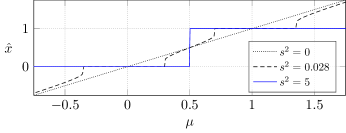
We observe that for given $\mu$ and a sufficiently large $s^{2}$, the estimate discretizes, i.e., $\hat{x}\in\{a,b\}$. For general $s^{2}$, however, (53) need not agree with (48) since the algorithm may converge to a local maximum (or a saddle point). This observation is summarized in the following theorem which guarantees that for sufficiently large $s^{2}$, the maximization in (48) is good-natured and (53) will converge to $a$ or $b$ (one of the solutions of  (48)), unless it is unluckily initialized to the (unavoidable) local minimum between $a$ and $b$.

• Theorem 3. The function

  $$x\mapsto\frac{\mathcal{N}\!\left({x;\mu,s^{2}}\right)}{|x-a|\cdot|x-b|}$$ (56)

  has no local maximum (other than the global maxima at $x=a$ and $x=b$) if and only if

  $$s^{2}>s^{2}_{\mathrm{AM}},$$ (57)

  where $s^{2}_{\mathrm{AM}}$ depends on $\mu,a$ and $b$. $\Box$

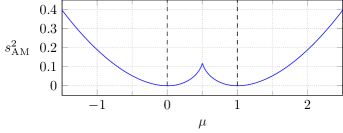
The proof of Theorem III-C4 (including the definition of $s^{2}_{\text{AM}}$) is lengthy and omitted here but can be found in [21]. Since $s^{2}_{\text{AM}}$ is the only real root of a cubic polynomial, a closed-form expression for $s^{2}_{\text{AM}}$ exists, but it is cumbersome. However, $s^{2}_{\text{AM}}$ is easily computed numerically. The value of $s^{2}_{\text{AM}}$ as a function of $\mu$ is plotted in Fig. 11. For example, $s_{\text{AM}}^{2}=0.028$ for $\mu=0.3$, $a=0$, and $b=1$ (cf. Fig. 10).

Figure 11: The value of $s^{2}_{\text{AM}}$ in (57) as a function of $\mu$, for $a=0$ and $b=1$.

III-C5 Type-II MAP Estimation

Another (and empirically much better) approach is to first form the MAP estimate

$$\hat{\theta} = \operatorname*{argmax}_{\theta}\int_{-\infty}^{\infty}p(\breve{y}\hskip 0.20004pt|\hskip 0.80002ptx)p(x,\theta)\,\mathop{}\!\mathrm{d}x,$$ (58)

after which we estimate $x$ by

$$\hat{x}=\operatorname*{argmax}_{x}p(\breve{y}\hskip 0.20004pt|\hskip 0.80002ptx)p(x,\hat{\theta}).$$ (59)

The difference to the joint MAP approach of Section III-C4 is the integration over $x$ in (58). Having in mind the generalization to the sequence setting of Section IV, we now consider computing (58) by expectation maximization (EM) [37] with hidden variable $X$, which operates by computing estimates $\hat{\theta}^{(1)},\hat{\theta}^{(2)},\,\ldots\,$ according to

$$\hat{\theta}^{(i)} = \operatorname*{argmax}_{\theta}\operatorname{\textnormal{$\mathbb{E}$}}\!\left[{\log\!\big{(}p(\breve{y}\hskip 0.20004pt|\hskip 0.80002ptX)p(X,\theta)\big{)}\rule{0.0pt}{8.61108pt}}\right]$$ (60)

$$= \operatorname*{argmax}_{\theta}\operatorname{\textnormal{$\mathbb{E}$}}\!\left[{\log p(X,\theta)\rule{0.0pt}{8.61108pt}}\right],$$ (61)

where the expectation is with respect to $p(x\hskip 0.20004pt|\hskip 0.80002pt\breve{y},\hat{\theta}^{(i-1)})$. The computation of (61) boils down to $\hat{\theta}^{(i)}=\left(\!\big{(}{{\hat{\sigma}_{a}}^{2}}\big{)}^{(i)},\big{(}{{\hat{\sigma}_{b}}^{2}}\big{)}^{(i)}\!\right)$ with

$$\big{(}{{\hat{\sigma}_{a}}^{2}}\big{)}^{(i)} = V_{X}^{(i)}+\big{(}\hat{x}^{(i)}-a\big{)}^{2}\quad\text{and}\quad$$ (62)

$$\big{(}{{\hat{\sigma}_{b}}^{2}}\big{)}^{(i)} = V_{X}^{(i)}+\big{(}\hat{x}^{(i)}-b\big{)}^{2}.$$ (63)

The derivation of (62) and (63) is detailed in Appendix A-C. Again, the maximizing variances (62) and (63) can be plugged into (18), resulting in

$$\mathchoice{\overarrow@\arrowfill@\relbar\relbar\smallrightarrow\displaystyle{V}}{\overarrow@\arrowfill@\relbar\relbar\smallrightarrow\textstyle{V}}{\overarrow@\arrowfill@\relbar\relbar\smallrightarrow\scriptstyle{V}}{\overarrow@\arrowfill@\relbar\relbar\smallrightarrow\scriptscriptstyle{V}}_{\mspace{-3.0mu}X} = \left(\frac{1}{V_{X}+(\hat{x}-a)^{2}}+\frac{1}{V_{X}+(\hat{x}-b)^{2}}\right)^{-1}$$ (64)

$$\mathchoice{\overarrow@\arrowfill@\relbar\relbar\smallrightarrow\displaystyle{m}}{\overarrow@\arrowfill@\relbar\relbar\smallrightarrow\textstyle{m}}{\overarrow@\arrowfill@\relbar\relbar\smallrightarrow\scriptstyle{m}}{\overarrow@\arrowfill@\relbar\relbar\smallrightarrow\scriptscriptstyle{m}}_{\mspace{-3.0mu}X} = \mathchoice{\overarrow@\arrowfill@\relbar\relbar\smallrightarrow\displaystyle{V}}{\overarrow@\arrowfill@\relbar\relbar\smallrightarrow\textstyle{V}}{\overarrow@\arrowfill@\relbar\relbar\smallrightarrow\scriptstyle{V}}{\overarrow@\arrowfill@\relbar\relbar\smallrightarrow\scriptscriptstyle{V}}_{\mspace{-3.0mu}X}\left(\frac{a}{V_{X}+(\hat{x}-a)^{2}}+\frac{b}{V_{X}+(\hat{x}-b)^{2}}\right),$$ (65)

where we have dropped the iteration index for readibility. The update rules (64) and (65) are given in Table II (in slightly different notation).

Computing (58) and afterwards (59) amounts to computing

$$\hat{x} = \operatorname*{argmax}_{x}p(\breve{y}\hskip 0.20004pt|\hskip 0.80002ptx)\mathcal{N}\!\left({x;\mathchoice{\overarrow@\arrowfill@\relbar\relbar\smallrightarrow\displaystyle{m}}{\overarrow@\arrowfill@\relbar\relbar\smallrightarrow\textstyle{m}}{\overarrow@\arrowfill@\relbar\relbar\smallrightarrow\scriptstyle{m}}{\overarrow@\arrowfill@\relbar\relbar\smallrightarrow\scriptscriptstyle{m}}_{\mspace{-3.0mu}X},\mathchoice{\overarrow@\arrowfill@\relbar\relbar\smallrightarrow\displaystyle{V}}{\overarrow@\arrowfill@\relbar\relbar\smallrightarrow\textstyle{V}}{\overarrow@\arrowfill@\relbar\relbar\smallrightarrow\scriptstyle{V}}{\overarrow@\arrowfill@\relbar\relbar\smallrightarrow\scriptscriptstyle{V}}_{\mspace{-3.0mu}X}}\right)$$ (66)

by iterating the two steps outlined in Section III-A2, except that $\mathchoice{\overarrow@\arrowfill@\relbar\relbar\smallrightarrow\displaystyle{m}}{\overarrow@\arrowfill@\relbar\relbar\smallrightarrow\textstyle{m}}{\overarrow@\arrowfill@\relbar\relbar\smallrightarrow\scriptstyle{m}}{\overarrow@\arrowfill@\relbar\relbar\smallrightarrow\scriptscriptstyle{m}}_{\mspace{-3.0mu}X}$ and $\mathchoice{\overarrow@\arrowfill@\relbar\relbar\smallrightarrow\displaystyle{V}}{\overarrow@\arrowfill@\relbar\relbar\smallrightarrow\textstyle{V}}{\overarrow@\arrowfill@\relbar\relbar\smallrightarrow\scriptstyle{V}}{\overarrow@\arrowfill@\relbar\relbar\smallrightarrow\scriptscriptstyle{V}}_{\mspace{-3.0mu}X}$ are updated according to (65) and (64), where the posterior variance is given by

$$V_{X}=\left(\frac{1}{\mathchoice{\overarrow@\arrowfill@\relbar\relbar\smallrightarrow\displaystyle{V}}{\overarrow@\arrowfill@\relbar\relbar\smallrightarrow\textstyle{V}}{\overarrow@\arrowfill@\relbar\relbar\smallrightarrow\scriptstyle{V}}{\overarrow@\arrowfill@\relbar\relbar\smallrightarrow\scriptscriptstyle{V}}_{\mspace{-3.0mu}X}}+\frac{1}{s^{2}}\right)^{-1}.$$ (67)

More specifically, we alternate the following two steps in iterations $i=1,2,3,\ldots$:

1. For fixed $\mathchoice{\overarrow@\arrowfill@\relbar\relbar\smallrightarrow\displaystyle{m}}{\overarrow@\arrowfill@\relbar\relbar\smallrightarrow\textstyle{m}}{\overarrow@\arrowfill@\relbar\relbar\smallrightarrow\scriptstyle{m}}{\overarrow@\arrowfill@\relbar\relbar\smallrightarrow\scriptscriptstyle{m}}_{\mspace{-3.0mu}X}^{(i-1)}$ and $\mathchoice{\overarrow@\arrowfill@\relbar\relbar\smallrightarrow\displaystyle{V}}{\overarrow@\arrowfill@\relbar\relbar\smallrightarrow\textstyle{V}}{\overarrow@\arrowfill@\relbar\relbar\smallrightarrow\scriptstyle{V}}{\overarrow@\arrowfill@\relbar\relbar\smallrightarrow\scriptscriptstyle{V}}_{\mspace{-3.0mu}X}^{(i-1)}$, compute the MAP estimate

   $$\hat{x}^{(i)} = \operatorname*{argmax}_{x}p(\breve{y}\hskip 0.20004pt|\hskip 0.80002ptx)\mathcal{N}\!\left({x;\mathchoice{\overarrow@\arrowfill@\relbar\relbar\smallrightarrow\displaystyle{m}}{\overarrow@\arrowfill@\relbar\relbar\smallrightarrow\textstyle{m}}{\overarrow@\arrowfill@\relbar\relbar\smallrightarrow\scriptstyle{m}}{\overarrow@\arrowfill@\relbar\relbar\smallrightarrow\scriptscriptstyle{m}}_{\mspace{-3.0mu}X}^{(i-1)},\mathchoice{\overarrow@\arrowfill@\relbar\relbar\smallrightarrow\displaystyle{V}}{\overarrow@\arrowfill@\relbar\relbar\smallrightarrow\textstyle{V}}{\overarrow@\arrowfill@\relbar\relbar\smallrightarrow\scriptstyle{V}}{\overarrow@\arrowfill@\relbar\relbar\smallrightarrow\scriptscriptstyle{V}}_{\mspace{-3.0mu}X}^{(i-1)}}\right)$$ (68)

   $$= \left(\frac{1}{\mathchoice{\overarrow@\arrowfill@\relbar\relbar\smallrightarrow\displaystyle{V}}{\overarrow@\arrowfill@\relbar\relbar\smallrightarrow\textstyle{V}}{\overarrow@\arrowfill@\relbar\relbar\smallrightarrow\scriptstyle{V}}{\overarrow@\arrowfill@\relbar\relbar\smallrightarrow\scriptscriptstyle{V}}_{\mspace{-3.0mu}X}^{(i-1)}}+\frac{1}{s^{2}}\right)^{-1}\!\!\left(\frac{\mathchoice{\overarrow@\arrowfill@\relbar\relbar\smallrightarrow\displaystyle{m}}{\overarrow@\arrowfill@\relbar\relbar\smallrightarrow\textstyle{m}}{\overarrow@\arrowfill@\relbar\relbar\smallrightarrow\scriptstyle{m}}{\overarrow@\arrowfill@\relbar\relbar\smallrightarrow\scriptscriptstyle{m}}_{\mspace{-3.0mu}X}^{(i-1)}}{\mathchoice{\overarrow@\arrowfill@\relbar\relbar\smallrightarrow\displaystyle{V}}{\overarrow@\arrowfill@\relbar\relbar\smallrightarrow\textstyle{V}}{\overarrow@\arrowfill@\relbar\relbar\smallrightarrow\scriptstyle{V}}{\overarrow@\arrowfill@\relbar\relbar\smallrightarrow\scriptscriptstyle{V}}_{\mspace{-3.0mu}X}^{(i-1)}}+\frac{\mu}{s^{2}}\right)\!.$$ (69)

2. For fixed $x=\hat{x}^{(i)}$, compute $\mathchoice{\overarrow@\arrowfill@\relbar\relbar\smallrightarrow\displaystyle{m}}{\overarrow@\arrowfill@\relbar\relbar\smallrightarrow\textstyle{m}}{\overarrow@\arrowfill@\relbar\relbar\smallrightarrow\scriptstyle{m}}{\overarrow@\arrowfill@\relbar\relbar\smallrightarrow\scriptscriptstyle{m}}_{\mspace{-3.0mu}X}^{(i)}$ and $\mathchoice{\overarrow@\arrowfill@\relbar\relbar\smallrightarrow\displaystyle{V}}{\overarrow@\arrowfill@\relbar\relbar\smallrightarrow\textstyle{V}}{\overarrow@\arrowfill@\relbar\relbar\smallrightarrow\scriptstyle{V}}{\overarrow@\arrowfill@\relbar\relbar\smallrightarrow\scriptscriptstyle{V}}_{\mspace{-3.0mu}X}^{(i)}$ according to (65) and (64).

Some numerical results of the estimate (66) are shown in Fig. 12.

Figure 12: The estimate (66) for $a=0$ and $b=1$, as a function of $\mu$. The unknown parameters were initialized to $\mathchoice{\overarrow@\arrowfill@\relbar\relbar\smallrightarrow\displaystyle{m}}{\overarrow@\arrowfill@\relbar\relbar\smallrightarrow\textstyle{m}}{\overarrow@\arrowfill@\relbar\relbar\smallrightarrow\scriptstyle{m}}{\overarrow@\arrowfill@\relbar\relbar\smallrightarrow\scriptscriptstyle{m}}_{\mspace{-3.0mu}X}^{(0)}=0$ and $\mathchoice{\overarrow@\arrowfill@\relbar\relbar\smallrightarrow\displaystyle{V}}{\overarrow@\arrowfill@\relbar\relbar\smallrightarrow\textstyle{V}}{\overarrow@\arrowfill@\relbar\relbar\smallrightarrow\scriptstyle{V}}{\overarrow@\arrowfill@\relbar\relbar\smallrightarrow\scriptscriptstyle{V}}_{\mspace{-3.0mu}X}^{(0)}=1$. For a given $\mu$ and sufficiently large $s^{2}$, the estimate $\hat{x}$ discretizes to the two levels $a$ and $b$.

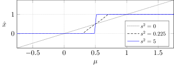
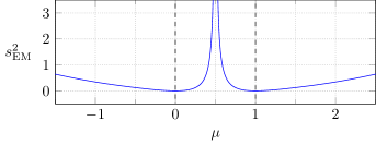
We observe that for a given $\mu$ and a sufficiently large $s^{2}$, the estimate discretizes, i.e., $\hat{x}\in\{a,b\}$. For general $s^{2}$ however, (66) need not agree with (59) since the algorithm may converge to a local maximum (or a saddle point). This observation is summarized in the following theorem which guarantees that for sufficiently large $s^{2}$, the maximization in (58) is good-natured and (59) returns $\hat{x}=a$ or $\hat{x}=b.$ Moreover (and in contrast to AM of Section III-C4), EM converges to $a$ if $\mu$ is closer to $a$ than to $b$, and to $b$ if $\mu$ is closer to $b$; this important property is probably the main reason for the empirical superiority of EM over AM.

• Theorem 4. Assume $a<b$. For $\mu<(a+b)/2$, the function

  $$\theta\mapsto\int_{-\infty}^{\infty}\mathcal{N}\!\left({x;\mu,s^{2}}\right)p(x,\theta)\mathop{}\!\mathrm{d}x$$ (70)

  has a maximum at ${\sigma_{a}^{2}}=0$ and ${\sigma_{b}^{2}}=(a-b)^{2}$ (resulting in $\hat{x}=a$) and no other extrema if and only if

  $$s^{2}>s_{\text{EM}}^{2},$$ (71)

  where

  $$s_{\text{EM}}^{2}\!=\!\left\{\begin{array}[]{ll}(3\!-\!\sqrt{8})(a\!-\!\mu)(b\!-\!\mu)&\text{if $\mu\!<\!a\!-\!\frac{|a\!-\!b|}{\sqrt{2}}$},\\ \frac{(a-\mu)^{2}|a-b|}{(a+b)-2\mu}&\text{if $a\!-\!\frac{|a\!-\!b|}{\sqrt{2}}\leq\mu\!<\!\frac{a\!+\!b}{2}$}.\end{array}\right.$$ (74)

  Likewise, for $\mu>(a+b)/2$, (70) has a maximum at ${\sigma_{b}^{2}}=0$ and ${\sigma_{a}^{2}}=(a-b)^{2}$ (resulting in $\hat{x}=b$) and no other extrema if and only if

  $$s^{2}>s_{\text{EM}}^{2},$$ (75)

  where

  $$s_{\text{EM}}^{2}\!=\!\left\{\begin{array}[]{ll}(3\!-\!\sqrt{8})(a\!-\!\mu)(b\!-\!\mu)&\text{if $\mu\!>\!b\!+\!\frac{|a\!-\!b|}{\sqrt{2}}$},\\ \frac{(b-\mu)^{2}|a-b|}{2\mu-(a+b)}&\text{if $\frac{a\!+\!b}{2}\!<\!\mu\leq b\!+\!\frac{|a\!-\!b|}{\sqrt{2}}$}.\end{array}\right.$$ (78)

  $\Box$

The proof is lengthy and omitted here but can be found in [21]. The value of $s_{\text{EM}}^{2}$ as a function of $\mu$ is plotted in Fig. 13. For example, $s_{\text{EM}}^{2}=0.225$ for $\mu=0.3$, $a=0$ and $b=1$ (cf. Fig. 12).

Figure 13: The value of $s_{\text{EM}}^{2}$ in (74) and (78) as a function of $\mu$ for $a=0$ and $b=1$.

III-D $M$-Level Prior

III-D1 A False Start

An obvious attempt to generalize (39) to more than two levels is

$$p(x,\theta)\triangleq\mathcal{N}\!\left({x;a,\sigma_{a}^{2}}\right)\mathcal{N}\!\left({x;b,\sigma_{b}^{2}}\right)\mathcal{N}\!\left({x;c,\sigma_{c}^{2}}\right)\cdots$$ (79)

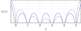
with $\theta\triangleq(\sigma_{a}^{2},\sigma_{b}^{2},\,\ldots)$. However, this turns out not to work very well since it introduces a bias towards the levels in the middle range. The effect is illustrated in Fig. 14, where the dashed line shows the generalization of (46) and Fig. 8 using $p(x,\theta)$ as in (79).

Figure 14: Generalization of (46) to $M=6$ equidistant levels. Solid blue: using (82) and (83). Dashed: using (79).

III-D2 Adding Binary Variables

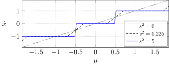
Good results are obtained with linear combinations of auxiliary binary (or binarized) variables. For example, constraining $X$ to three levels $\{-b,0,b\}$ can be achieved by writing

$$X=bX_{1}-bX_{2}$$ (80)

where both $X_{1}$ and $X_{2}$ are constrained to $\{0,1\}$ by means of independent priors (39), i.e.,

$$p(x_{1},x_{2},\theta_{1},\theta_{2}) = \mathcal{N}\!\left({x_{1};0,\sigma_{1,a}^{2}}\right)\mathcal{N}\!\left({x_{1};1,\sigma_{1,b}^{2}}\right)$$ (81)

$$\cdot\mathcal{N}\!\left({x_{2};0,\sigma_{2,a}^{2}}\right)\mathcal{N}\!\left({x_{2};1,\sigma_{2,b}^{2}}\right).$$

The corresponding generalization of Fig. 12 is shown as solid line in Fig. 15.

More generally, we can write $X$ as a linear combination

$$X=\sum_{j=1}^{J}\beta_{j}X_{j}+\beta_{0}$$ (82)

of independent binary (i.e., binarized to $\{0,1\}$) variables $X_{1},\,\ldots,X_{J}$. The choice of $J$ and of the coefficients $\beta_{0},\,\ldots,\beta_{J}$ is highly nonunique. Choosing $\beta_{j}=2^{j-1}$ for $j>0$ does not work well empirically. Good results are obtained with

$$\beta_{1}=\ldots=\beta_{J},$$ (83)

resulting in $M=J+1$ equidistant levels for $X$. (Related representations were used in [38].) The corresponding generalization of (46) is illustrated in Fig. 14 (solid blue line).

Figure 15: Generalization of Fig. 12 to three levels $\{-1,0,1\}$ using (80).

III-D3 Symmetry Breaking

In (82), $X_{1}=0$ and $X_{2}=1$ has the same effect on $X$ as $X_{1}=1$ and $X_{2}=0$. The estimation algorithm must somehow choose among such equivalent configurations. However, depending on the details of the implementation, the estimation algorithm may not, by itself, be able to break such symmetries. This problem can be solved by a slightly asymmetric initialization of the variances, e.g.,

$$\sigma_{1,a}^{2}=\sigma_{1,b}^{2}\neq\sigma_{2,a}^{2}=\sigma_{2,b}^{2},$$ (84)

where the inequality is almost an equality.

IV Linear State Space Models with NUV Priors

IV-A System Model

We will use the statistical system model (86), which is a generalization of the standard linear Gaussian state space model. We begin with the latter.

IV-A1 Standard Linear Gaussian Model

Recall the standard linear state space model (LSSM)

$$x_{k} = Ax_{k-1}+Bu_{k}$$ (85a)

$$y_{k} = Cx_{k}$$ (85b)

with time index $k\in\mathbb{N}$, initial state $x_{0}\in\mathbb{R}^{N}$, input $u_{k}\in\mathbb{R}^{L}$, state $x_{k}\in\mathbb{R}^{N}$, output $y_{k}\in\mathbb{R}^{H}$, input dimension $L\in\mathbb{N}$, state dimension $N\in\mathbb{N}$ and output dimension $H\in\mathbb{N}$. Further, we have the input matrix $B\in\mathbb{R}^{N\times L}$, the state transition matrix $A\in\mathbb{R}^{N\times N}$, and the observation matrix $C\in\mathbb{R}^{H\times N}$. For the sake of clarity, we here assume a time-invariant state space model; however, the proposed approach works also for time-varying state space models (with $A,B,C$ depending on $k$) and the pertinent generalizations are straightforward.

For the remainder of this paper, we assume a finite planning horizon $k\in\{1,\dots,K\}$.

The standard linear Gaussian model is obtained by turning the variables in (85a) into random variables (denoted by capitals) as follows. First, $U_{1},\dots,U_{K}$ are assumed to be independent Gaussian random variables; second, for $k\in\{1,\dots,K\}$ we observe $\breve{Y}_{k}=Y_{k}+Z_{k}$, where $Z_{1},\dots,Z_{K}$ are independent zero-mean Gaussian random variables that model the measurement noise. For fixed observations $\breve{Y}_{1}=\breve{y}_{1},\dots,\breve{Y}_{K}=\breve{y}_{K}$, the joint posterior probability density of all other variables can then be written as

$$p(u,x,y\hskip 0.20004pt|\hskip 0.80002pt\breve{y})\propto p(x_{0})\prod_{k=1}^{K}p(u_{k})p(\breve{y}_{k}\hskip 0.20004pt|\hskip 0.80002pty_{k})\bigg{\rvert}_{\text{(\ref{eqn:lssm:detLSSM})}}$$ (86)

with $u\triangleq\begin{bmatrix}u_{1},\dots,u_{K}\end{bmatrix}$, $x\triangleq\begin{bmatrix}x_{0},\dots,x_{K}\end{bmatrix}$, $y\triangleq\begin{bmatrix}y_{1},\dots,y_{K}\end{bmatrix}$, and $\breve{y}\triangleq\begin{bmatrix}\breve{y}_{1},\dots,\breve{y}_{K}\end{bmatrix}$.

IV-A2 Linear Gaussian Model with NUV Parameters

We will work with the generalization of (86) to

$$p(y,x,u;\theta)\!\propto\!\mathchoice{\overarrow@\arrowfill@\relbar\relbar\smallrightarrow\displaystyle{p}}{\overarrow@\arrowfill@\relbar\relbar\smallrightarrow\textstyle{p}}{\overarrow@\arrowfill@\relbar\relbar\smallrightarrow\scriptstyle{p}}{\overarrow@\arrowfill@\relbar\relbar\smallrightarrow\scriptscriptstyle{p}}_{\mspace{-3.0mu}}(x_{0})\!\left(\prod_{k=1}^{K}\mathchoice{\overarrow@\arrowfill@\relbar\relbar\smallrightarrow\displaystyle{p}}{\overarrow@\arrowfill@\relbar\relbar\smallrightarrow\textstyle{p}}{\overarrow@\arrowfill@\relbar\relbar\smallrightarrow\scriptstyle{p}}{\overarrow@\arrowfill@\relbar\relbar\smallrightarrow\scriptscriptstyle{p}}_{\mspace{-3.0mu}}(u_{k};\theta_{U_{k}})\mathchoice{\overarrow@\arrowfill@\smallleftarrow\relbar\relbar\displaystyle{p}}{\overarrow@\arrowfill@\smallleftarrow\relbar\relbar\textstyle{p}}{\overarrow@\arrowfill@\smallleftarrow\relbar\relbar\scriptstyle{p}}{\overarrow@\arrowfill@\smallleftarrow\relbar\relbar\scriptscriptstyle{p}}_{\mspace{-3.0mu}}(y_{k};\theta_{Y_{k}})\!\!\right)\mathchoice{\overarrow@\arrowfill@\smallleftarrow\relbar\relbar\displaystyle{p}}{\overarrow@\arrowfill@\smallleftarrow\relbar\relbar\textstyle{p}}{\overarrow@\arrowfill@\smallleftarrow\relbar\relbar\scriptstyle{p}}{\overarrow@\arrowfill@\smallleftarrow\relbar\relbar\scriptscriptstyle{p}}_{\mspace{-3.0mu}}(x_{K})\bigg{\rvert}_{\text{(\ref{eqn:lssm:detLSSM})}}$$

(as illustrated in Fig. 16), where $\mathchoice{\overarrow@\arrowfill@\relbar\relbar\smallrightarrow\displaystyle{p}}{\overarrow@\arrowfill@\relbar\relbar\smallrightarrow\textstyle{p}}{\overarrow@\arrowfill@\relbar\relbar\smallrightarrow\scriptstyle{p}}{\overarrow@\arrowfill@\relbar\relbar\smallrightarrow\scriptscriptstyle{p}}_{\mspace{-3.0mu}}(u_{k};\theta_{U_{k}})$ is Gaussian with parameters $\theta_{U_{k}}\triangleq(\mathchoice{\overarrow@\arrowfill@\relbar\relbar\smallrightarrow\displaystyle{m}}{\overarrow@\arrowfill@\relbar\relbar\smallrightarrow\textstyle{m}}{\overarrow@\arrowfill@\relbar\relbar\smallrightarrow\scriptstyle{m}}{\overarrow@\arrowfill@\relbar\relbar\smallrightarrow\scriptscriptstyle{m}}_{\mspace{-3.0mu}U_{k}},\mathchoice{\overarrow@\arrowfill@\relbar\relbar\smallrightarrow\displaystyle{V}}{\overarrow@\arrowfill@\relbar\relbar\smallrightarrow\textstyle{V}}{\overarrow@\arrowfill@\relbar\relbar\smallrightarrow\scriptstyle{V}}{\overarrow@\arrowfill@\relbar\relbar\smallrightarrow\scriptscriptstyle{V}}_{\mspace{-3.0mu}U_{k}})$, $\mathchoice{\overarrow@\arrowfill@\smallleftarrow\relbar\relbar\displaystyle{p}}{\overarrow@\arrowfill@\smallleftarrow\relbar\relbar\textstyle{p}}{\overarrow@\arrowfill@\smallleftarrow\relbar\relbar\scriptstyle{p}}{\overarrow@\arrowfill@\smallleftarrow\relbar\relbar\scriptscriptstyle{p}}_{\mspace{-3.0mu}}(y_{k};\theta_{Y_{k}})$ is Gaussian with parameters $\theta_{Y_{k}}\triangleq(\mathchoice{\overarrow@\arrowfill@\smallleftarrow\relbar\relbar\displaystyle{m}}{\overarrow@\arrowfill@\smallleftarrow\relbar\relbar\textstyle{m}}{\overarrow@\arrowfill@\smallleftarrow\relbar\relbar\scriptstyle{m}}{\overarrow@\arrowfill@\smallleftarrow\relbar\relbar\scriptscriptstyle{m}}_{\mspace{-3.0mu}Y_{k}},\mathchoice{\overarrow@\arrowfill@\smallleftarrow\relbar\relbar\displaystyle{V}}{\overarrow@\arrowfill@\smallleftarrow\relbar\relbar\textstyle{V}}{\overarrow@\arrowfill@\smallleftarrow\relbar\relbar\scriptstyle{V}}{\overarrow@\arrowfill@\smallleftarrow\relbar\relbar\scriptscriptstyle{V}}_{\mspace{-3.0mu}Y_{k}})$, and $\theta\triangleq(\theta_{U_{1}},\dots,\theta_{U_{K}},\theta_{Y_{1}}\dots,\theta_{Y_{K}})$. Note that the special case (86) is obtained with $\mathchoice{\overarrow@\arrowfill@\relbar\relbar\smallrightarrow\displaystyle{p}}{\overarrow@\arrowfill@\relbar\relbar\smallrightarrow\textstyle{p}}{\overarrow@\arrowfill@\relbar\relbar\smallrightarrow\scriptstyle{p}}{\overarrow@\arrowfill@\relbar\relbar\smallrightarrow\scriptscriptstyle{p}}_{\mspace{-3.0mu}}(x_{0})=p(x_{0})$, $\mathchoice{\overarrow@\arrowfill@\relbar\relbar\smallrightarrow\displaystyle{p}}{\overarrow@\arrowfill@\relbar\relbar\smallrightarrow\textstyle{p}}{\overarrow@\arrowfill@\relbar\relbar\smallrightarrow\scriptstyle{p}}{\overarrow@\arrowfill@\relbar\relbar\smallrightarrow\scriptscriptstyle{p}}_{\mspace{-3.0mu}}(u_{k};\theta_{U_{k}})=p(u_{k})$, $\mathchoice{\overarrow@\arrowfill@\smallleftarrow\relbar\relbar\displaystyle{p}}{\overarrow@\arrowfill@\smallleftarrow\relbar\relbar\textstyle{p}}{\overarrow@\arrowfill@\smallleftarrow\relbar\relbar\scriptstyle{p}}{\overarrow@\arrowfill@\smallleftarrow\relbar\relbar\scriptscriptstyle{p}}_{\mspace{-3.0mu}}(y_{k};\theta_{Y_{k}})=p(\breve{y}_{k}\hskip 0.20004pt|\hskip 0.80002pty_{k})$, where the observations $\breve{y}_{k}$ are subsumed in $\theta_{Y_{k}}$, and $\mathchoice{\overarrow@\arrowfill@\smallleftarrow\relbar\relbar\displaystyle{p}}{\overarrow@\arrowfill@\smallleftarrow\relbar\relbar\textstyle{p}}{\overarrow@\arrowfill@\smallleftarrow\relbar\relbar\scriptstyle{p}}{\overarrow@\arrowfill@\smallleftarrow\relbar\relbar\scriptscriptstyle{p}}_{\mspace{-3.0mu}}(x_{K})=1$.

If the inputs $U_{k}$ and the outputs $Y_{k}$ are scalars (i.e., $L=H=1$), every factor $\mathchoice{\overarrow@\arrowfill@\relbar\relbar\smallrightarrow\displaystyle{p}}{\overarrow@\arrowfill@\relbar\relbar\smallrightarrow\textstyle{p}}{\overarrow@\arrowfill@\relbar\relbar\smallrightarrow\scriptstyle{p}}{\overarrow@\arrowfill@\relbar\relbar\smallrightarrow\scriptscriptstyle{p}}_{\mspace{-3.0mu}}(u_{k};\theta_{U_{k}})$ and $\mathchoice{\overarrow@\arrowfill@\smallleftarrow\relbar\relbar\displaystyle{p}}{\overarrow@\arrowfill@\smallleftarrow\relbar\relbar\textstyle{p}}{\overarrow@\arrowfill@\smallleftarrow\relbar\relbar\scriptstyle{p}}{\overarrow@\arrowfill@\smallleftarrow\relbar\relbar\scriptscriptstyle{p}}_{\mspace{-3.0mu}}(y_{k};\theta_{Y_{k}})$ can be a NUV prior; in particular, these factors can be used to impose any of the constraints discussed in Section III on any input $U_{k}$ or any output $Y_{k}$. If $L>1$ or $H>1$, NUV priors on scalar components of $U_{k}$ and $Y_{k}$ can easily be included in $\mathchoice{\overarrow@\arrowfill@\relbar\relbar\smallrightarrow\displaystyle{p}}{\overarrow@\arrowfill@\relbar\relbar\smallrightarrow\textstyle{p}}{\overarrow@\arrowfill@\relbar\relbar\smallrightarrow\scriptstyle{p}}{\overarrow@\arrowfill@\relbar\relbar\smallrightarrow\scriptscriptstyle{p}}_{\mspace{-3.0mu}}(u_{k};\theta_{U_{k}})$ and $\mathchoice{\overarrow@\arrowfill@\smallleftarrow\relbar\relbar\displaystyle{p}}{\overarrow@\arrowfill@\smallleftarrow\relbar\relbar\textstyle{p}}{\overarrow@\arrowfill@\smallleftarrow\relbar\relbar\scriptstyle{p}}{\overarrow@\arrowfill@\smallleftarrow\relbar\relbar\scriptscriptstyle{p}}_{\mspace{-3.0mu}}(y_{k};\theta_{Y_{k}})$.

Concerning the initial state, we assume $\mathchoice{\overarrow@\arrowfill@\relbar\relbar\smallrightarrow\displaystyle{p}}{\overarrow@\arrowfill@\relbar\relbar\smallrightarrow\textstyle{p}}{\overarrow@\arrowfill@\relbar\relbar\smallrightarrow\scriptstyle{p}}{\overarrow@\arrowfill@\relbar\relbar\smallrightarrow\scriptscriptstyle{p}}_{\mspace{-3.0mu}}(x_{0})$ to be Gaussian with known mean $\mathchoice{\overarrow@\arrowfill@\relbar\relbar\smallrightarrow\displaystyle{m}}{\overarrow@\arrowfill@\relbar\relbar\smallrightarrow\textstyle{m}}{\overarrow@\arrowfill@\relbar\relbar\smallrightarrow\scriptstyle{m}}{\overarrow@\arrowfill@\relbar\relbar\smallrightarrow\scriptscriptstyle{m}}_{\mspace{-3.0mu}X_{0}}$ and covariance matrix $\mathchoice{\overarrow@\arrowfill@\relbar\relbar\smallrightarrow\displaystyle{V}}{\overarrow@\arrowfill@\relbar\relbar\smallrightarrow\textstyle{V}}{\overarrow@\arrowfill@\relbar\relbar\smallrightarrow\scriptstyle{V}}{\overarrow@\arrowfill@\relbar\relbar\smallrightarrow\scriptscriptstyle{V}}_{\mspace{-3.0mu}X_{0}}$. Concerning the terminal state, we assume either $\mathchoice{\overarrow@\arrowfill@\smallleftarrow\relbar\relbar\displaystyle{p}}{\overarrow@\arrowfill@\smallleftarrow\relbar\relbar\textstyle{p}}{\overarrow@\arrowfill@\smallleftarrow\relbar\relbar\scriptstyle{p}}{\overarrow@\arrowfill@\smallleftarrow\relbar\relbar\scriptscriptstyle{p}}_{\mspace{-3.0mu}}(x_{K})=1$ or else that $\mathchoice{\overarrow@\arrowfill@\smallleftarrow\relbar\relbar\displaystyle{p}}{\overarrow@\arrowfill@\smallleftarrow\relbar\relbar\textstyle{p}}{\overarrow@\arrowfill@\smallleftarrow\relbar\relbar\scriptstyle{p}}{\overarrow@\arrowfill@\smallleftarrow\relbar\relbar\scriptscriptstyle{p}}_{\mspace{-3.0mu}}(x_{K})$ is Gaussian with known mean $\mathchoice{\overarrow@\arrowfill@\smallleftarrow\relbar\relbar\displaystyle{m}}{\overarrow@\arrowfill@\smallleftarrow\relbar\relbar\textstyle{m}}{\overarrow@\arrowfill@\smallleftarrow\relbar\relbar\scriptstyle{m}}{\overarrow@\arrowfill@\smallleftarrow\relbar\relbar\scriptscriptstyle{m}}_{\mspace{-3.0mu}X_{K}}$ and covariance matrix $\mathchoice{\overarrow@\arrowfill@\smallleftarrow\relbar\relbar\displaystyle{V}}{\overarrow@\arrowfill@\smallleftarrow\relbar\relbar\textstyle{V}}{\overarrow@\arrowfill@\smallleftarrow\relbar\relbar\scriptstyle{V}}{\overarrow@\arrowfill@\smallleftarrow\relbar\relbar\scriptscriptstyle{V}}_{\mspace{-3.0mu}X_{K}}$.

Figure 16: Factor graph of the model (IV-A2).

IV-B Iterative Augmented Kalman Estimation (IAKE)

For fixed parameters $\theta$, the variables $U,X,Y$ in (IV-A2) are jointly Gaussian, and the MAP estimate of any subset of these variables coincides with their (posterior) mean. For the joint estimation of $U,Y$, and all NUV parameters in $\theta$, we will use the following algorithm. The final MAP estimate of $U$ (when the algorithm stops) is the desired control signal $\hat{u}=\begin{bmatrix}\hat{u}_{1},\dots,\hat{u}_{K}\end{bmatrix}$.

Starting from an initial guess $\hat{\theta}^{(0)}$, the algorithm repeats the following two steps for $i=1,2,3,\ldots,$ until convergence (or for a sufficiently large number of iterations):

1. For fixed $\theta=\hat{\theta}^{(i-1)}$, compute for $k\in\{1,\dots,K\}$

   1. the posterior means $m_{U_{k}}^{(i)}$ (and, if necessary, the posterior variances $V_{U_{k}}^{(i)}$) of $U_{k}$,

   2. the posterior means $m_{Y_{k}}^{(i)}$ (and, if necessary, the posterior variances $V_{Y_{k}}^{(i)}$) of $Y_{k}$.

2. From these means and variances, determine new parameters $\theta^{(i)}$ using Tables I and II.

These two steps are repeated until some convergence criterion is satisfied (e.g., some fixed number of iterations).

Note that Step i) operates with a standard linear Gaussian model. In consequence, the required means and variances can be computed by Kalman-type recursions or, equivalently, by forward-backward Gaussian message passing, with a complexity that is linear in $K$.

A preferred such algorithm is the MBF smoother [39] augmented with input signal estimation as in [15, 8]. This algorithm requires no matrix inversion and is numerically stable. For the convenience of readers unfamiliar with the setting of [8], the algorithm is concisely stated in Table III.

The algorithm consists of a forward recursion followed by a backward recursion. The former is a standard Kalman filter, but the latter is not quite standard. Initialize $\mathchoice{\overarrow@\arrowfill@\relbar\relbar\smallrightarrow\displaystyle{m}}{\overarrow@\arrowfill@\relbar\relbar\smallrightarrow\textstyle{m}}{\overarrow@\arrowfill@\relbar\relbar\smallrightarrow\scriptstyle{m}}{\overarrow@\arrowfill@\relbar\relbar\smallrightarrow\scriptscriptstyle{m}}_{\mspace{-3.0mu}X_{0}}$, $\mathchoice{\overarrow@\arrowfill@\relbar\relbar\smallrightarrow\displaystyle{V}}{\overarrow@\arrowfill@\relbar\relbar\smallrightarrow\textstyle{V}}{\overarrow@\arrowfill@\relbar\relbar\smallrightarrow\scriptstyle{V}}{\overarrow@\arrowfill@\relbar\relbar\smallrightarrow\scriptscriptstyle{V}}_{\mspace{-3.0mu}X_{0}}$, $\mathchoice{\overarrow@\arrowfill@\smallleftarrow\relbar\relbar\displaystyle{m}}{\overarrow@\arrowfill@\smallleftarrow\relbar\relbar\textstyle{m}}{\overarrow@\arrowfill@\smallleftarrow\relbar\relbar\scriptstyle{m}}{\overarrow@\arrowfill@\smallleftarrow\relbar\relbar\scriptscriptstyle{m}}_{\mspace{-3.0mu}X_{K}}$, $\mathchoice{\overarrow@\arrowfill@\smallleftarrow\relbar\relbar\displaystyle{V}}{\overarrow@\arrowfill@\smallleftarrow\relbar\relbar\textstyle{V}}{\overarrow@\arrowfill@\smallleftarrow\relbar\relbar\scriptstyle{V}}{\overarrow@\arrowfill@\smallleftarrow\relbar\relbar\scriptscriptstyle{V}}_{\mspace{-3.0mu}X_{K}}$ according to Section IV-A2. Forward recursion: For $k=1,2,\dots,K$, compute $\displaystyle\mathchoice{\overarrow@\arrowfill@\relbar\relbar\smallrightarrow\displaystyle{m}}{\overarrow@\arrowfill@\relbar\relbar\smallrightarrow\textstyle{m}}{\overarrow@\arrowfill@\relbar\relbar\smallrightarrow\scriptstyle{m}}{\overarrow@\arrowfill@\relbar\relbar\smallrightarrow\scriptscriptstyle{m}}_{\mspace{-3.0mu}X_{k}^{\prime}}$ $\displaystyle=$ $\displaystyle A\mathchoice{\overarrow@\arrowfill@\relbar\relbar\smallrightarrow\displaystyle{m}}{\overarrow@\arrowfill@\relbar\relbar\smallrightarrow\textstyle{m}}{\overarrow@\arrowfill@\relbar\relbar\smallrightarrow\scriptstyle{m}}{\overarrow@\arrowfill@\relbar\relbar\smallrightarrow\scriptscriptstyle{m}}_{\mspace{-3.0mu}X_{k-1}}+B\mathchoice{\overarrow@\arrowfill@\relbar\relbar\smallrightarrow\displaystyle{m}}{\overarrow@\arrowfill@\relbar\relbar\smallrightarrow\textstyle{m}}{\overarrow@\arrowfill@\relbar\relbar\smallrightarrow\scriptstyle{m}}{\overarrow@\arrowfill@\relbar\relbar\smallrightarrow\scriptscriptstyle{m}}_{\mspace{-3.0mu}U_{k}}$ (F.1) $\displaystyle\mathchoice{\overarrow@\arrowfill@\relbar\relbar\smallrightarrow\displaystyle{V}}{\overarrow@\arrowfill@\relbar\relbar\smallrightarrow\textstyle{V}}{\overarrow@\arrowfill@\relbar\relbar\smallrightarrow\scriptstyle{V}}{\overarrow@\arrowfill@\relbar\relbar\smallrightarrow\scriptscriptstyle{V}}_{\mspace{-3.0mu}X_{k}^{\prime}}$ $\displaystyle=$ $\displaystyle A\mathchoice{\overarrow@\arrowfill@\relbar\relbar\smallrightarrow\displaystyle{V}}{\overarrow@\arrowfill@\relbar\relbar\smallrightarrow\textstyle{V}}{\overarrow@\arrowfill@\relbar\relbar\smallrightarrow\scriptstyle{V}}{\overarrow@\arrowfill@\relbar\relbar\smallrightarrow\scriptscriptstyle{V}}_{\mspace{-3.0mu}X_{k-1}}A^{{\mathsf{T}}}+B\mathchoice{\overarrow@\arrowfill@\relbar\relbar\smallrightarrow\displaystyle{V}}{\overarrow@\arrowfill@\relbar\relbar\smallrightarrow\textstyle{V}}{\overarrow@\arrowfill@\relbar\relbar\smallrightarrow\scriptstyle{V}}{\overarrow@\arrowfill@\relbar\relbar\smallrightarrow\scriptscriptstyle{V}}_{\mspace{-3.0mu}U_{k}}B^{{\mathsf{T}}}$ (F.2) $\displaystyle\mathchoice{\overarrow@\arrowfill@\relbar\relbar\smallrightarrow\displaystyle{m}}{\overarrow@\arrowfill@\relbar\relbar\smallrightarrow\textstyle{m}}{\overarrow@\arrowfill@\relbar\relbar\smallrightarrow\scriptstyle{m}}{\overarrow@\arrowfill@\relbar\relbar\smallrightarrow\scriptscriptstyle{m}}_{\mspace{-3.0mu}X_{k}}$ $\displaystyle=$ $\displaystyle\mathchoice{\overarrow@\arrowfill@\relbar\relbar\smallrightarrow\displaystyle{m}}{\overarrow@\arrowfill@\relbar\relbar\smallrightarrow\textstyle{m}}{\overarrow@\arrowfill@\relbar\relbar\smallrightarrow\scriptstyle{m}}{\overarrow@\arrowfill@\relbar\relbar\smallrightarrow\scriptscriptstyle{m}}_{\mspace{-3.0mu}X_{k}^{\prime}}+\mathchoice{\overarrow@\arrowfill@\relbar\relbar\smallrightarrow\displaystyle{V}}{\overarrow@\arrowfill@\relbar\relbar\smallrightarrow\textstyle{V}}{\overarrow@\arrowfill@\relbar\relbar\smallrightarrow\scriptstyle{V}}{\overarrow@\arrowfill@\relbar\relbar\smallrightarrow\scriptscriptstyle{V}}_{\mspace{-3.0mu}X_{k}^{\prime}}E_{k}$ (F.3) $\displaystyle\mathchoice{\overarrow@\arrowfill@\relbar\relbar\smallrightarrow\displaystyle{V}}{\overarrow@\arrowfill@\relbar\relbar\smallrightarrow\textstyle{V}}{\overarrow@\arrowfill@\relbar\relbar\smallrightarrow\scriptstyle{V}}{\overarrow@\arrowfill@\relbar\relbar\smallrightarrow\scriptscriptstyle{V}}_{\mspace{-3.0mu}X_{k}}$ $\displaystyle=$ $\displaystyle F_{k}\mathchoice{\overarrow@\arrowfill@\relbar\relbar\smallrightarrow\displaystyle{V}}{\overarrow@\arrowfill@\relbar\relbar\smallrightarrow\textstyle{V}}{\overarrow@\arrowfill@\relbar\relbar\smallrightarrow\scriptstyle{V}}{\overarrow@\arrowfill@\relbar\relbar\smallrightarrow\scriptscriptstyle{V}}_{\mspace{-3.0mu}X_{k}^{\prime}}$ (F.4) $\displaystyle E_{k}$ $\displaystyle=$ $\displaystyle C^{{\mathsf{T}}}G_{k}(\mathchoice{\overarrow@\arrowfill@\smallleftarrow\relbar\relbar\displaystyle{m}}{\overarrow@\arrowfill@\smallleftarrow\relbar\relbar\textstyle{m}}{\overarrow@\arrowfill@\smallleftarrow\relbar\relbar\scriptstyle{m}}{\overarrow@\arrowfill@\smallleftarrow\relbar\relbar\scriptscriptstyle{m}}_{\mspace{-3.0mu}Y_{k}}-C\mathchoice{\overarrow@\arrowfill@\relbar\relbar\smallrightarrow\displaystyle{m}}{\overarrow@\arrowfill@\relbar\relbar\smallrightarrow\textstyle{m}}{\overarrow@\arrowfill@\relbar\relbar\smallrightarrow\scriptstyle{m}}{\overarrow@\arrowfill@\relbar\relbar\smallrightarrow\scriptscriptstyle{m}}_{\mspace{-3.0mu}X_{k}^{\prime}})$ (F.5) $\displaystyle F_{k}$ $\displaystyle=$ $\displaystyle I_{N}-\mathchoice{\overarrow@\arrowfill@\relbar\relbar\smallrightarrow\displaystyle{V}}{\overarrow@\arrowfill@\relbar\relbar\smallrightarrow\textstyle{V}}{\overarrow@\arrowfill@\relbar\relbar\smallrightarrow\scriptstyle{V}}{\overarrow@\arrowfill@\relbar\relbar\smallrightarrow\scriptscriptstyle{V}}_{\mspace{-3.0mu}X_{k}^{\prime}}C^{{\mathsf{T}}}G_{k}C$ (F.6) $\displaystyle G_{k}$ $\displaystyle=$ $\displaystyle(\mathchoice{\overarrow@\arrowfill@\smallleftarrow\relbar\relbar\displaystyle{V}}{\overarrow@\arrowfill@\smallleftarrow\relbar\relbar\textstyle{V}}{\overarrow@\arrowfill@\smallleftarrow\relbar\relbar\scriptstyle{V}}{\overarrow@\arrowfill@\smallleftarrow\relbar\relbar\scriptscriptstyle{V}}_{\mspace{-3.0mu}Y_{k}}+C\mathchoice{\overarrow@\arrowfill@\relbar\relbar\smallrightarrow\displaystyle{V}}{\overarrow@\arrowfill@\relbar\relbar\smallrightarrow\textstyle{V}}{\overarrow@\arrowfill@\relbar\relbar\smallrightarrow\scriptstyle{V}}{\overarrow@\arrowfill@\relbar\relbar\smallrightarrow\scriptscriptstyle{V}}_{\mspace{-3.0mu}X_{k}^{\prime}}C^{{\mathsf{T}}})^{-1}.$ (F.7) Backward recursion: Initialize with $\tilde{W}_{X_{K}}\!=0_{N\times N}$ and $\tilde{\xi}_{X_{K}}\!=0_{N}$ if $\mathchoice{\overarrow@\arrowfill@\smallleftarrow\relbar\relbar\displaystyle{p}}{\overarrow@\arrowfill@\smallleftarrow\relbar\relbar\textstyle{p}}{\overarrow@\arrowfill@\smallleftarrow\relbar\relbar\scriptstyle{p}}{\overarrow@\arrowfill@\smallleftarrow\relbar\relbar\scriptscriptstyle{p}}_{\mspace{-3.0mu}(X_{K})}=1$, else $\displaystyle\tilde{W}_{X_{K}}$ $\displaystyle=$ $\displaystyle(\mathchoice{\overarrow@\arrowfill@\relbar\relbar\smallrightarrow\displaystyle{V}}{\overarrow@\arrowfill@\relbar\relbar\smallrightarrow\textstyle{V}}{\overarrow@\arrowfill@\relbar\relbar\smallrightarrow\scriptstyle{V}}{\overarrow@\arrowfill@\relbar\relbar\smallrightarrow\scriptscriptstyle{V}}_{\mspace{-3.0mu}X_{K}}+\mathchoice{\overarrow@\arrowfill@\smallleftarrow\relbar\relbar\displaystyle{V}}{\overarrow@\arrowfill@\smallleftarrow\relbar\relbar\textstyle{V}}{\overarrow@\arrowfill@\smallleftarrow\relbar\relbar\scriptstyle{V}}{\overarrow@\arrowfill@\smallleftarrow\relbar\relbar\scriptscriptstyle{V}}_{\mspace{-3.0mu}X_{K}})^{-1}$ (B.1) $\displaystyle\tilde{\xi}_{X_{K}}$ $\displaystyle=$ $\displaystyle\tilde{W}_{X_{K}}(\mathchoice{\overarrow@\arrowfill@\relbar\relbar\smallrightarrow\displaystyle{m}}{\overarrow@\arrowfill@\relbar\relbar\smallrightarrow\textstyle{m}}{\overarrow@\arrowfill@\relbar\relbar\smallrightarrow\scriptstyle{m}}{\overarrow@\arrowfill@\relbar\relbar\smallrightarrow\scriptscriptstyle{m}}_{\mspace{-3.0mu}X_{K}}-\mathchoice{\overarrow@\arrowfill@\smallleftarrow\relbar\relbar\displaystyle{m}}{\overarrow@\arrowfill@\smallleftarrow\relbar\relbar\textstyle{m}}{\overarrow@\arrowfill@\smallleftarrow\relbar\relbar\scriptstyle{m}}{\overarrow@\arrowfill@\smallleftarrow\relbar\relbar\scriptscriptstyle{m}}_{\mspace{-3.0mu}X_{K}}).\hskip 13.00005pt$ (B.2) For $k=K,K-1,\dots,1$, compute $\displaystyle\tilde{\xi}_{X_{k}^{\prime}}$ $\displaystyle=$ $\displaystyle F_{k}^{{\mathsf{T}}}\tilde{\xi}_{X_{k}}-E_{k}$ (B.3) $\displaystyle\tilde{W}_{X_{k}^{\prime}}$ $\displaystyle=$ $\displaystyle F_{k}^{{\mathsf{T}}}\tilde{W}_{X_{k}}F_{k}+C^{{\mathsf{T}}}G_{k}C\hskip 20.00003pt$ (B.4) $\displaystyle\tilde{\xi}_{X_{k-1}}$ $\displaystyle=$ $\displaystyle A^{{\mathsf{T}}}\tilde{\xi}_{X_{k}^{\prime}}$ (B.5) $\displaystyle\tilde{W}_{X_{k-1}}$ $\displaystyle=$ $\displaystyle A^{{\mathsf{T}}}\tilde{W}_{X_{k}^{\prime}}A.$ (B.6) Posterior quantities: The posterior means and variances for $k\in\{1,\dots,K\}$ are given by $\displaystyle m_{U_{k}}$ $\displaystyle=$ $\displaystyle\mathchoice{\overarrow@\arrowfill@\relbar\relbar\smallrightarrow\displaystyle{m}}{\overarrow@\arrowfill@\relbar\relbar\smallrightarrow\textstyle{m}}{\overarrow@\arrowfill@\relbar\relbar\smallrightarrow\scriptstyle{m}}{\overarrow@\arrowfill@\relbar\relbar\smallrightarrow\scriptscriptstyle{m}}_{\mspace{-3.0mu}U_{k}}-\mathchoice{\overarrow@\arrowfill@\relbar\relbar\smallrightarrow\displaystyle{V}}{\overarrow@\arrowfill@\relbar\relbar\smallrightarrow\textstyle{V}}{\overarrow@\arrowfill@\relbar\relbar\smallrightarrow\scriptstyle{V}}{\overarrow@\arrowfill@\relbar\relbar\smallrightarrow\scriptscriptstyle{V}}_{\mspace{-3.0mu}U_{k}}B^{{\mathsf{T}}}\tilde{\xi}_{X_{k}^{\prime}}$ (P.1) $\displaystyle V_{U_{k}}$ $\displaystyle=$ $\displaystyle\mathchoice{\overarrow@\arrowfill@\relbar\relbar\smallrightarrow\displaystyle{V}}{\overarrow@\arrowfill@\relbar\relbar\smallrightarrow\textstyle{V}}{\overarrow@\arrowfill@\relbar\relbar\smallrightarrow\scriptstyle{V}}{\overarrow@\arrowfill@\relbar\relbar\smallrightarrow\scriptscriptstyle{V}}_{\mspace{-3.0mu}U_{k}}-\mathchoice{\overarrow@\arrowfill@\relbar\relbar\smallrightarrow\displaystyle{V}}{\overarrow@\arrowfill@\relbar\relbar\smallrightarrow\textstyle{V}}{\overarrow@\arrowfill@\relbar\relbar\smallrightarrow\scriptstyle{V}}{\overarrow@\arrowfill@\relbar\relbar\smallrightarrow\scriptscriptstyle{V}}_{\mspace{-3.0mu}U_{k}}B^{{\mathsf{T}}}\tilde{W}_{X_{k}^{\prime}}B\mathchoice{\overarrow@\arrowfill@\relbar\relbar\smallrightarrow\displaystyle{V}}{\overarrow@\arrowfill@\relbar\relbar\smallrightarrow\textstyle{V}}{\overarrow@\arrowfill@\relbar\relbar\smallrightarrow\scriptstyle{V}}{\overarrow@\arrowfill@\relbar\relbar\smallrightarrow\scriptscriptstyle{V}}_{\mspace{-3.0mu}U_{k}}$ (P.2) $\displaystyle m_{Y_{k}}$ $\displaystyle=$ $\displaystyle C\left(\mathchoice{\overarrow@\arrowfill@\relbar\relbar\smallrightarrow\displaystyle{m}}{\overarrow@\arrowfill@\relbar\relbar\smallrightarrow\textstyle{m}}{\overarrow@\arrowfill@\relbar\relbar\smallrightarrow\scriptstyle{m}}{\overarrow@\arrowfill@\relbar\relbar\smallrightarrow\scriptscriptstyle{m}}_{\mspace{-3.0mu}X_{k}}-\mathchoice{\overarrow@\arrowfill@\relbar\relbar\smallrightarrow\displaystyle{V}}{\overarrow@\arrowfill@\relbar\relbar\smallrightarrow\textstyle{V}}{\overarrow@\arrowfill@\relbar\relbar\smallrightarrow\scriptstyle{V}}{\overarrow@\arrowfill@\relbar\relbar\smallrightarrow\scriptscriptstyle{V}}_{\mspace{-3.0mu}X_{k}}\tilde{\xi}_{X_{k}}\right)$ (P.3) $\displaystyle V_{Y_{k}}$ $\displaystyle=$ $\displaystyle C\left(\mathchoice{\overarrow@\arrowfill@\relbar\relbar\smallrightarrow\displaystyle{V}}{\overarrow@\arrowfill@\relbar\relbar\smallrightarrow\textstyle{V}}{\overarrow@\arrowfill@\relbar\relbar\smallrightarrow\scriptstyle{V}}{\overarrow@\arrowfill@\relbar\relbar\smallrightarrow\scriptscriptstyle{V}}_{\mspace{-3.0mu}X_{k}}-\mathchoice{\overarrow@\arrowfill@\relbar\relbar\smallrightarrow\displaystyle{V}}{\overarrow@\arrowfill@\relbar\relbar\smallrightarrow\textstyle{V}}{\overarrow@\arrowfill@\relbar\relbar\smallrightarrow\scriptstyle{V}}{\overarrow@\arrowfill@\relbar\relbar\smallrightarrow\scriptscriptstyle{V}}_{\mspace{-3.0mu}X_{k}}\tilde{W}_{X_{k}}\mathchoice{\overarrow@\arrowfill@\relbar\relbar\smallrightarrow\displaystyle{V}}{\overarrow@\arrowfill@\relbar\relbar\smallrightarrow\textstyle{V}}{\overarrow@\arrowfill@\relbar\relbar\smallrightarrow\scriptstyle{V}}{\overarrow@\arrowfill@\relbar\relbar\smallrightarrow\scriptscriptstyle{V}}_{\mspace{-3.0mu}X_{k}}\right)C^{{\mathsf{T}}}.$ (P.4)

TABLE III: Step i) of IAKE implemented by MBF message passing with input estimation assembled from [8].

Concerning Step ii), we note that the derivations of the update rules in Section III are easily adapted to the system model (IV-A2); in particular, the estimation of all NUV parameters in (IV-A2) splits into separate individual estimates, each as in Tables I and II.

In practice, often only a subset of (P.1)–(P.4) needs to be computed, depending on the problem at hand and the relevant update rules in Tables I and II.

We also note that this algorithm is easily adapted to mildly nonlinear systems, cf. Section V-E.

V Application Examples

V-A Digital-To-Analog Conversion

We now describe Example II of Section II in detail. For the numerical experiments, the physical system is a simple analog low-pass filter with transfer function (i.e., the Laplace transform of the impulse response)

$$G(s)=\frac{35037.9}{s^{3}+71.9s^{2}+2324.8s+35037.9}.$$ (88)

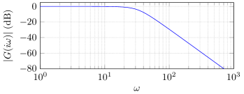
The amplitude response (i.e., the magnitude of the frequency response $G(i\omega)$) of this filter is shown in Fig. 17. (Such low-order filters cannot be good low-pass filters, but they are inexpensive by all relevant measures.)

Figure 17: Frequency response of (88).

The transfer function (88) is transformed into state-space form and discretized using a sampling interval of $T=0.003$ seconds, resulting in a discrete-time LSSM as in (85a) with state space dimension $N=3$ and matrices

$$A\! = \!\begin{bmatrix}0.7967&-6.3978&-94.2123\\ 0.0027&0.9902&-0.1467\\ 0&0.0030&0.9999\end{bmatrix},\;B\!=\!\begin{bmatrix}0.0027\\ 0\\ 0\end{bmatrix},$$ (89a)

and

$$C = \begin{bmatrix}0&0&35037.9\end{bmatrix}.$$ (90a)

Recall that we wish to compute a binary input signal $u$, such that the model output $y$ approximates a given target waveform $\breve{y}$. We reformulate the constrained optimization problem (3a) as a statistical estimation problem using a linear Gaussian model with NUV parameters (see Section IV-A2) as follows: The quadratic penalty (3a) is readily expressed by (7) with fixed parameters $\mathchoice{\overarrow@\arrowfill@\smallleftarrow\relbar\relbar\displaystyle{m}}{\overarrow@\arrowfill@\smallleftarrow\relbar\relbar\textstyle{m}}{\overarrow@\arrowfill@\smallleftarrow\relbar\relbar\scriptstyle{m}}{\overarrow@\arrowfill@\smallleftarrow\relbar\relbar\scriptscriptstyle{m}}_{\mspace{-3.0mu}Y_{k}}=\breve{y}_{k}$ and $\mathchoice{\overarrow@\arrowfill@\smallleftarrow\relbar\relbar\displaystyle{V}}{\overarrow@\arrowfill@\smallleftarrow\relbar\relbar\textstyle{V}}{\overarrow@\arrowfill@\smallleftarrow\relbar\relbar\scriptstyle{V}}{\overarrow@\arrowfill@\smallleftarrow\relbar\relbar\scriptscriptstyle{V}}_{\mspace{-3.0mu}Y_{k}}>0$. The binary input constraint (3b) is expressed by (6) with unknown parameters $\mathchoice{\overarrow@\arrowfill@\relbar\relbar\smallrightarrow\displaystyle{m}}{\overarrow@\arrowfill@\relbar\relbar\smallrightarrow\textstyle{m}}{\overarrow@\arrowfill@\relbar\relbar\smallrightarrow\scriptstyle{m}}{\overarrow@\arrowfill@\relbar\relbar\smallrightarrow\scriptscriptstyle{m}}_{\mspace{-3.0mu}U_{k}}$ and $\mathchoice{\overarrow@\arrowfill@\relbar\relbar\smallrightarrow\displaystyle{V}}{\overarrow@\arrowfill@\relbar\relbar\smallrightarrow\textstyle{V}}{\overarrow@\arrowfill@\relbar\relbar\smallrightarrow\scriptstyle{V}}{\overarrow@\arrowfill@\relbar\relbar\smallrightarrow\scriptscriptstyle{V}}_{\mspace{-3.0mu}U_{k}}$. The estimation problem is then solved using the IAKE algorithm proposed in Section IV-B:

In Step i) of the algorithm (Table III), we compute $m_{U_{k}}^{(i)}$ and $V_{U_{k}}^{(i)}$, for $k\in\{1,\dots,K\}$, using (P.1) and (P.2), where $i$ is the iteration index. In Step ii) of the algorithm, we determine the unknown parameters $\theta^{(i)}$ using Table II. Specifically, the parameters $\mathchoice{\overarrow@\arrowfill@\relbar\relbar\smallrightarrow\displaystyle{m}}{\overarrow@\arrowfill@\relbar\relbar\smallrightarrow\textstyle{m}}{\overarrow@\arrowfill@\relbar\relbar\smallrightarrow\scriptstyle{m}}{\overarrow@\arrowfill@\relbar\relbar\smallrightarrow\scriptscriptstyle{m}}_{\mspace{-3.0mu}U_{k}}^{(i)}$ and $\mathchoice{\overarrow@\arrowfill@\relbar\relbar\smallrightarrow\displaystyle{V}}{\overarrow@\arrowfill@\relbar\relbar\smallrightarrow\textstyle{V}}{\overarrow@\arrowfill@\relbar\relbar\smallrightarrow\scriptstyle{V}}{\overarrow@\arrowfill@\relbar\relbar\smallrightarrow\scriptscriptstyle{V}}_{\mspace{-3.0mu}U_{k}}^{(i)}$ are updated according to the last row of Table II, with $m_{X}=m_{U_{k}}^{(i)}$, $V_{X}=V_{U_{k}}^{(i)}$, $a=0$ and $b=1$. The final estimate of $U$ is

$$\hat{u}=\begin{bmatrix}m_{U_{1}}^{(i)},\ldots,m_{U_{K}}^{(i)}\end{bmatrix},$$ (91)

where $i$ is the final iteration.

The numerical results shown in Fig. 2 are obtained with $\mathchoice{\overarrow@\arrowfill@\smallleftarrow\relbar\relbar\displaystyle{V}}{\overarrow@\arrowfill@\smallleftarrow\relbar\relbar\textstyle{V}}{\overarrow@\arrowfill@\smallleftarrow\relbar\relbar\scriptstyle{V}}{\overarrow@\arrowfill@\smallleftarrow\relbar\relbar\scriptscriptstyle{V}}_{\mspace{-3.0mu}Y_{k}}=0.045$ and $K=450$. Note that $\mathchoice{\overarrow@\arrowfill@\smallleftarrow\relbar\relbar\displaystyle{V}}{\overarrow@\arrowfill@\smallleftarrow\relbar\relbar\textstyle{V}}{\overarrow@\arrowfill@\smallleftarrow\relbar\relbar\scriptstyle{V}}{\overarrow@\arrowfill@\smallleftarrow\relbar\relbar\scriptscriptstyle{V}}_{\mspace{-3.0mu}Y_{k}}$ controls the approximation quality as it scales the weight of the squared error between $y$ and $\breve{y}$. The first half of Fig. 2 shows the nominal operation of the digital-to-analog converter, where the target waveform can be well approximated. The second half of Fig. 2 illustrates what happens if the (unreasonable) target waveform falls outside the passband of the analog filter.

V-A1 Comparison With Other Methods

The global minimum of (3a) can, in principle, be determined by an exhaustive search. However, the complexity of such a search is exponential in the planning horizon $K$, which limits its practicability to small $K$. (Smart versions of tree search such as sphere decoding suffer from the same fundamental limitation.)

By contrast, the algorithm proposed in Section IV-B will normally converge to a local, rather than the global, maximum of (3a). However, in many applications, this deficiency is far outweighed by the ability to easily handle large $K$.

Figure 18: Comparing the proposed method (with planning horizon $K=200$) with an optimal (exhaustive search) controller with planning horizon $K=8$. The former yields a significantly better approximation ($y$ with $\text{MSE}=0.01972$) than the latter ($y^{*}$ with $\text{MSE}=0.04885$).

Figure 19: Comparing the proposed method with planning horizon $K=8$ with an optimal controller with the same planning horizon. The former yields almost as good a solution ($y$ with $\text{MSE}=0.04899$) as the latter ($y^{*}$ with $\text{MSE}=0.04885$).

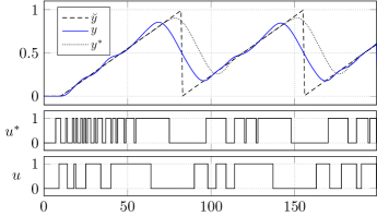
For example, Fig. 18 compares an “optimal” (exhaustive search) controller with planning horizon $K=8$ with the proposed algorithm. The analog system is the same (3rd-order low-pass) as in Section V-A. The results are obtained with $\mathchoice{\overarrow@\arrowfill@\smallleftarrow\relbar\relbar\displaystyle{V}}{\overarrow@\arrowfill@\smallleftarrow\relbar\relbar\textstyle{V}}{\overarrow@\arrowfill@\smallleftarrow\relbar\relbar\scriptstyle{V}}{\overarrow@\arrowfill@\smallleftarrow\relbar\relbar\scriptscriptstyle{V}}_{\mspace{-3.0mu}Y_{k}}=0.01$ and full-length $K$. It is obvious from Fig. 18 that the ability to look sufficiently far ahead is crucial for good performance.

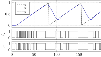
But how suboptimal is the proposed algorithm really? Fig. 19 shows the performance of the proposed algorithm in online mode with the same planning horizon $K=8$ as the exhaustive-search controller: it turns out, in this example, that the proposed algorithm is very nearly optimal.

V-B Corridor Control with Different Input Constraints

Assume we wish to keep the model output $y$ within a corridor around a target $\breve{y}$, i.e., we wish $y_{k}$ to satisfy

$$a_{k}\leq y_{k}-\breve{y}_{k}\leq b_{k},\quad k\in\{1,\dots,K\},$$ (92)

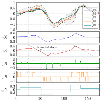
for fixed bounds $a_{k},b_{k}\in\mathbb{R}$. We can achieve this by $\mathchoice{\overarrow@\arrowfill@\smallleftarrow\relbar\relbar\displaystyle{p}}{\overarrow@\arrowfill@\smallleftarrow\relbar\relbar\textstyle{p}}{\overarrow@\arrowfill@\smallleftarrow\relbar\relbar\scriptstyle{p}}{\overarrow@\arrowfill@\smallleftarrow\relbar\relbar\scriptscriptstyle{p}}_{\mspace{-3.0mu}}(y_{k};\theta_{Y_{k}})$ implementing (the NUV realization of) a box constraint on $Y_{k}$ as in Section III-A, with bounds $a_{k}+\breve{y}_{k}$ and $b_{k}+\breve{y}_{k}$, and slope parameter $\gamma_{o}$. In the following, we consider five different version of this problem, with different constraints on the control signal $u$:

In version 1, the input $u$ is constrained by an $L_{2}$ penalty.

In version 2, the discrete derivative of the input $u$ is constrained to satisfy $\Delta u_{k}\geq-0.03$ (by a half-space prior as in Section III-B). Constraining the derivative instead of the input itself is easily handled by a small modification of (85a); the augmented model amounts to

$$\tilde{A}=\begin{bmatrix}1&0_{1\times N}\\ B&A\end{bmatrix},\;\tilde{B}=\begin{bmatrix}1\\ 0_{N\times 1}\end{bmatrix},\;\text{and}\;\;\tilde{C}=\begin{bmatrix}0&C\end{bmatrix}.$$ (93)

In version 3, the input $u$ is constrained to be sparse (by a sparsifying NUV prior [8], which empirically works better than standard $L_{1}$ regularization [32]).

In version 4, the input $u$ is constrained to be discrete-valued, i.e., to satisfy $u_{k}\in\{-1,0,1\}$ (by an $M$-level prior as in Section III-D2 using EM).

In version 5, the discrete derivative of the input $u$ is constrained to be sparse (by a sparsifying NUV prior [8]).

Note that version 3, 4 and 5 are nonconvex problems. A variation of version 3 was also discussed in [40].

The numerical results in Fig. 20 are obtained with the following state space model

$$A = \begin{bmatrix}1&0&0\\ 1&1&0\\ 1/2&1&1\end{bmatrix},\quad B=0.0015\begin{bmatrix}1\\ 1/2\\ 1/3\end{bmatrix},$$ (94a)

and

$$C=\begin{bmatrix}0&0&1\end{bmatrix}.$$ (95a)

Furthermore, we have $K=175$, $\lambda_{o}=10$ for the box prior on the output, $\mathchoice{\overarrow@\arrowfill@\relbar\relbar\smallrightarrow\displaystyle{m}}{\overarrow@\arrowfill@\relbar\relbar\smallrightarrow\textstyle{m}}{\overarrow@\arrowfill@\relbar\relbar\smallrightarrow\scriptstyle{m}}{\overarrow@\arrowfill@\relbar\relbar\smallrightarrow\scriptscriptstyle{m}}_{\mspace{-3.0mu}U_{k}}=0$ and $\mathchoice{\overarrow@\arrowfill@\relbar\relbar\smallrightarrow\displaystyle{V}}{\overarrow@\arrowfill@\relbar\relbar\smallrightarrow\textstyle{V}}{\overarrow@\arrowfill@\relbar\relbar\smallrightarrow\scriptstyle{V}}{\overarrow@\arrowfill@\relbar\relbar\smallrightarrow\scriptscriptstyle{V}}_{\mspace{-3.0mu}U_{k}}=10$ in version 1, and $a_{i}=-0.03$ and $\lambda_{i}=10$ for the half-space prior on the input in version 2. The corresponding inputs and outputs are illustrated using different colors. The bounds of the corridor are indicated by dashed lines in the first plot.

Figure 20: Corridor control with different constraints on the input. Top row: allowed corridor (dashed) and output signals. Second row: input $u$ with $L_{2}$ penalty. Third row: input $u$ with constraint on its derivative. Fourth row: input $u$ with sparsifying penalty. Fifth row: input $u$ constrained to three levels. Bottom row: input $u$ with sparsifying penalty on its derivative.

V-C Flappy Bird Control

The following control problem is a variation of the flappy bird computer game [41]. (This example improves on the related example in [19], which did not use box constraints.)

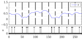
Consider a physical system consisting of a point mass $m$ moving forward (left to right in Fig. 21) with constant horizontal velocity and “falling” vertically with constant acceleration $g$. The $\{0,1\}$-valued control signal $u$ affects the system only if $u_{k}=1$, in which case a fixed value is added to the vertical momentum. We wish to steer the point mass such that it passes through a sequence of double slits, and hence, does not collide with the obstacles (black bars in Fig. 21).

For this example, we need a slight generalization of (85a) as follows. The state $x_{k}\in\mathbb{R}^{2}$ (comprising the vertical position and the vertical velocity) evolves according to

$$x_{k} = \begin{bmatrix}1&T\\ 0&1\end{bmatrix}x_{k-1}+\begin{bmatrix}0\\ 1/m\end{bmatrix}u_{k}+\begin{bmatrix}0\\ -Tg\end{bmatrix}.$$ (96)

Let $\mathcal{S}\subset\{1,\ldots,K\}$ be the positions of the double slits. For $k\in\mathcal{S}$, we have the augmented output

$$\tilde{y}_{k}=\begin{bmatrix}1&0\end{bmatrix}x_{k}+s_{k},$$ (97)

where $s_{k}\in\{0,d_{k}\}$ “selects” either the lower or the upper slit, and where ${d_{k}\in\mathbb{R}}$ specifies the vertical distance between them. The double-slit constraint (98) is achieved by a box constraint on $\tilde{Y}_{k}$ (with bounds $a_{k}$ and $b_{k}$) and a binarizing constraint on $S_{k}$. By doing so, the vertical position $y_{k}\triangleq\begin{bmatrix}1&0\end{bmatrix}x_{k}$ is constrained to satisfy

$$y_{k}\in[a_{k},b_{k}]\quad\text{or}\quad y_{k}\in[a_{k}-d_{k},b_{k}-d_{k}].$$ (98)

In addition, we use a binarizing prior on $U_{k}$ with levels $\{0,1\}$ for all $k$.

The numerical results in Fig. 21 are obtained with $K=300$, $m=1$, $T=0.1$, $g=0.2$, $\gamma=100$, and $a_{k},b_{k}$ and $d_{k}$ according to Fig. 21.

Figure 21: Double-slit flappy bird control with binary control signal $u$, and resulting trajectory $y$, which must not collide with the obstacles (black bars).

V-D Trajectory Planning with Obstacle Avoidance

Consider the following situation. An object is moving in a two-dimensional plane. Its position at time $k$ is $y_{k}=\begin{bmatrix}y_{k,1},y_{k,2}\end{bmatrix}^{\mathsf{T}}\in\mathbb{R}^{2}$, which is governed by the state space model (85a) with

$$A = \begin{bmatrix}1&0&0&0\\ T&1&0&0\\ 0&0&1&0\\ 0&0&T&1\end{bmatrix},\;B=\begin{bmatrix}T\\ 0\\ T\\ 0\end{bmatrix},\;\text{and}\;\;C=\begin{bmatrix}0\\ 1\\ 0\\ 1\end{bmatrix}^{\mathsf{T}}\!,$$ (99)

where $T$ is the discretization interval and $u_{k}=\begin{bmatrix}u_{k,1},u_{k,2}\end{bmatrix}^{\mathsf{T}}$ is the acceleration.

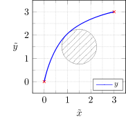
Assume we wish to plan a trajectory starting from $\begin{bmatrix}0,0\end{bmatrix}^{\mathsf{T}}$ (with zero velocity) and ending at $\begin{bmatrix}3,3\end{bmatrix}^{\mathsf{T}}$ (with zero velocity), while avoiding a spherical obstacle at $c=\begin{bmatrix}1.5,1.5\end{bmatrix}^{\mathsf{T}}$ with radius $r=0.75$ (see Fig. 23(a)). In addition, we wish to minimize the squared norm of the acceleration, i.e.,

$$\sum_{k=1}^{K}\|u_{k}\|^{2},$$ (100)

which is easily handled by a zero-mean Gaussian prior on $U_{k}$, for all $k$.

The obstacle can be avoided by a half-space constraint on the auxiliary variable

$$\tilde{z}_{k}\triangleq\|y_{k}-c\|=f(y_{k}),\quad k\in\{1,\dots,K\},$$ (101)

which is the distance from $y_{k}$ to the center $c$ of the obstacle. Specifically, we use a half-space NUV prior to enforce

$$\tilde{z}_{k}>r.$$ (102)

It remains to deal with the problem that (101) is a nonlinear function of $y_{k}$. We solve this problem in the most obvious way, by using the linearization

$$z_{k}=f(y_{k}^{*})+\nabla f(y_{k}^{*})(y_{k}-y_{k}^{*})\approx f(y_{k})$$ (103)

(as illustrated in Fig. 22), where $y_{k}^{*}\in\mathbb{R}^{2}$ is the previous estimate of $Y_{k}$ and $\nabla f(y_{k}^{*})$ is the gradient of $f$ at $y_{k}=y_{k}^{*}$.

Figure 22: Factor graph representation of the modified observation model with half-space prior $p(z_{k};\theta_{k})$.

The numerical results illustrated in Fig. 23(a) are obtained with $T=1$, $\gamma=5$, $\mathchoice{\overarrow@\arrowfill@\relbar\relbar\smallrightarrow\displaystyle{m}}{\overarrow@\arrowfill@\relbar\relbar\smallrightarrow\textstyle{m}}{\overarrow@\arrowfill@\relbar\relbar\smallrightarrow\scriptstyle{m}}{\overarrow@\arrowfill@\relbar\relbar\smallrightarrow\scriptscriptstyle{m}}_{\mspace{-3.0mu}U_{k}}=\begin{bmatrix}0,0\end{bmatrix}^{\mathsf{T}}$, $\mathchoice{\overarrow@\arrowfill@\relbar\relbar\smallrightarrow\displaystyle{V}}{\overarrow@\arrowfill@\relbar\relbar\smallrightarrow\textstyle{V}}{\overarrow@\arrowfill@\relbar\relbar\smallrightarrow\scriptstyle{V}}{\overarrow@\arrowfill@\relbar\relbar\smallrightarrow\scriptscriptstyle{V}}_{\mspace{-3.0mu}U_{k}}=\operatorname{diag}\left(0.1,0.1\right)$, and boundary conditions

$$\mathchoice{\overarrow@\arrowfill@\relbar\relbar\smallrightarrow\displaystyle{m}}{\overarrow@\arrowfill@\relbar\relbar\smallrightarrow\textstyle{m}}{\overarrow@\arrowfill@\relbar\relbar\smallrightarrow\scriptstyle{m}}{\overarrow@\arrowfill@\relbar\relbar\smallrightarrow\scriptscriptstyle{m}}_{\mspace{-3.0mu}X_{0}} = \begin{bmatrix}0,0,0,0\end{bmatrix}^{\mathsf{T}},$$ (104)

$$\mathchoice{\overarrow@\arrowfill@\smallleftarrow\relbar\relbar\displaystyle{m}}{\overarrow@\arrowfill@\smallleftarrow\relbar\relbar\textstyle{m}}{\overarrow@\arrowfill@\smallleftarrow\relbar\relbar\scriptstyle{m}}{\overarrow@\arrowfill@\smallleftarrow\relbar\relbar\scriptscriptstyle{m}}_{\mspace{-3.0mu}X_{K}} = \begin{bmatrix}0,3,0,3\end{bmatrix}^{\mathsf{T}},\quad\text{and}$$ (105)

$$\mathchoice{\overarrow@\arrowfill@\relbar\relbar\smallrightarrow\displaystyle{V}}{\overarrow@\arrowfill@\relbar\relbar\smallrightarrow\textstyle{V}}{\overarrow@\arrowfill@\relbar\relbar\smallrightarrow\scriptstyle{V}}{\overarrow@\arrowfill@\relbar\relbar\smallrightarrow\scriptscriptstyle{V}}_{\mspace{-3.0mu}X_{0}} = \mathchoice{\overarrow@\arrowfill@\smallleftarrow\relbar\relbar\displaystyle{V}}{\overarrow@\arrowfill@\smallleftarrow\relbar\relbar\textstyle{V}}{\overarrow@\arrowfill@\smallleftarrow\relbar\relbar\scriptstyle{V}}{\overarrow@\arrowfill@\smallleftarrow\relbar\relbar\scriptscriptstyle{V}}_{\mspace{-3.0mu}X_{K}}=0_{4\times 4}.$$ (106)

Note that the optimal solution of the given problem is not unique since the problem is geometrically symmetric. The obtained solution depends on the initial conditions.

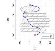
The method of this example is easily extended to multiple obstacles by concatenating multiple instances of the part shown in Fig. 22. The method is not limited to spherical obstacles as long as the nonlinearity of $f$ is good-natured. Ellipses, squares, rectangles, and linear transformations (e.g., scaling and rotations) thereof have been successfully implemented by choosing $f$ accordingly. An example with multiple obstacles of various shapes is given in Fig. 23(b), the details are omitted.

V-E Minimal-Time Race Track Control

Autonomous racing is a version of autonomous driving where the goal is to complete a given race track in the shortest time possible. The following challenges must be dealt with:

• Nonlinear vehicle dynamics.

• Physical limitations of the vehicle such as maximal steering angle and maximal motor torque.

• Collision avoidance with track boundaries.

Several methods to solve this control problem have been proposed in the literature [42, 43, 44]. We now show how this problem can be addressed with the approach of this paper. As recommended in the literature, we will use a curvilinear coordinate system [45, 46, 47, 48], which simplifies expressing the constraints imposed by the track boundaries.

(a)

(b)

Figure 23: (a) Trajectory planning with a single spherical obstacle at $\begin{bmatrix}1.5,1.5\end{bmatrix}^{\mathsf{T}}$. Note that the optimal trajectory $y$ is not unique. (b) Trajectory planning with obstacles of various shapes. The obtained trajectory $y$ is only locally optimal.

We begin by describing the vehicle dynamics using the standard Ackermann vehicle model [49] in Cartesian coordinates $\tilde{x}$ and $\tilde{y}$, from which the final state space model will be obtained in a series of transformations. The model consists of the differential equation

$$\frac{\mathop{}\!\mathrm{d}x}{\mathop{}\!\mathrm{d}t}=f(x(t),u(t))=\begin{bmatrix}v(t)\cos(\theta(t))\\ v(t)\sin(\theta(t))\\ v(t)\frac{\tan(\delta(t))}{\ell}\\ a(t)\\ \dot{a}(t)\\ \dot{\delta}(t)\end{bmatrix}$$ (107)

with state

$$x(t)=\begin{bmatrix}\tilde{x}(t),\tilde{y}(t),\theta(t),v(t),a(t),\delta(t)\end{bmatrix}^{\mathsf{T}}$$ (108)

and input

$$u(t)=\begin{bmatrix}\dot{\delta}(t)\\ \dot{a}(t)\end{bmatrix},$$ (109)

and with steering angle $\delta$ (front wheel, back wheel is fixed), vehicle length $\ell$, heading angle $\theta$, speed $v$, and acceleration $a$.

In a next step, we transform this state space model into a curvilinear coordinate system as illustrated in Fig. 24.

Figure 24: Curvilinear coordinate system, where $s$ is the progress on the center line, $z$ is the vehicle’s displacement perpendicular to the centerline, and $\theta$ is the heading angle relative to a tangent vector at $s$.

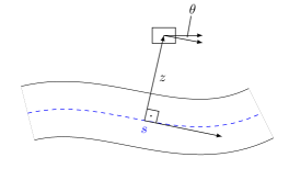
The first coordinate $s$ (of the curvilinear coordinate system) describes the progress along the center line of the race track, whereas the second coordinate $z$ describes the perpendicular deviation of the vehicle with respect to the center line at $s$. The angle $\theta$ instances the angle between the vehicle’s direction of travel and the tangent vector at $s$. Consequently, the state vector is

$$x(t)=\begin{bmatrix}s(t),z(t),\theta(t),v(t),a(t),\delta(t)\end{bmatrix}^{\mathsf{T}}.$$ (110)

The vehicle dynamics (107) in the curvilinear coordinates turn out to be

$$\frac{\mathop{}\!\mathrm{d}x}{\mathop{}\!\mathrm{d}t}=f_{t}(x(t),u(t))=\begin{bmatrix}v\frac{\cos(\theta)}{{1-\kappa(s)z}}\\ v\sin(\theta)\\ v\left(\frac{\tan(\delta)}{\ell}-\frac{\kappa(s)\cos(\theta)}{{1-\kappa(s)z}}\right)\\ a\\ \dot{a}\\ \dot{\delta}\end{bmatrix},$$ (111)

where $\kappa(s)$ is the curvature of the center line. Note that the right-hand side of (111) depends on the time $t$, which is omitted for readability.

In (111), the independent variable is time, and hence, formulating a minimal-time optimization problem is nontrivial. We therefore transform the state space model once more, into a form where $s$ is the independent variable. The transformed model follows directly from

$$\frac{\mathop{}\!\mathrm{d}x}{\mathop{}\!\mathrm{d}s} = \frac{\mathop{}\!\mathrm{d}x}{\mathop{}\!\mathrm{d}t}\frac{\mathop{}\!\mathrm{d}t}{\mathop{}\!\mathrm{d}s}=\left(\frac{\mathop{}\!\mathrm{d}s}{\mathop{}\!\mathrm{d}t}\right)^{-1}\frac{\mathop{}\!\mathrm{d}x}{\mathop{}\!\mathrm{d}t}$$ (112)

$$= \left(\frac{{1-\kappa(s)z}}{v\cos(\theta)}\right)f_{t}(x(s),u(s)).$$ (113)

Accordingly, the new state and input vectors are no longer functions of $t$, but functions of $s$, i.e., $x(s)$, and $u(s)$, respectively. Since $s$ is now the independent variable, we drop the first state and add time as an additional state, i.e.,

$$x(s)=\begin{bmatrix}z(s),\theta(s),v(s),a(s),\delta(s),t(s)\end{bmatrix}^{\mathsf{T}}.$$ (114)

The new model dynamics are

$$\frac{\mathop{}\!\mathrm{d}x}{\mathop{}\!\mathrm{d}s}\!=\!f_{s}(x(s),u(s))\!=\!\frac{1\!-\!\kappa(s)z}{v\cos(\theta)}\!\begin{bmatrix}v\sin(\theta)\\ v\!\left(\!\frac{\tan(\delta)}{\ell}\!-\!\frac{\cos(\theta)}{\kappa(s)^{-1}\!-\!z}\!\right)\!\!\\ a\\ \dot{a}\\ \dot{\delta}\\ 1\end{bmatrix}\!.$$ (115)

In order to impose suitable state constraints, we define

$$y(s)=f_{o}(x(s))=\begin{bmatrix}z\\ a\\ \delta\\ a^{2}+\psi\frac{v^{4}}{\ell^{2}}\tan(\delta)^{2}\end{bmatrix},$$ (116)

where the last component of (116) is the squared total acceleration $a_{\text{tot}}^{2}$, and where $\psi$ is a weighting factor to incorporate all unmodeled physical properties of the vehicle. Keeping the vehicle within the track boundaries is achieved by imposing a box constraint on the vehicle’s deviation from the center line $z$. Further box constraints on the longitudinal acceleration $a$ and the steering angle $\delta$ enforce physical limitations of the vehicle. Finally, a box constraint on the total acceleration $a_{\text{tot}}^{2}$ prevents the vehicle from slipping.

Figure 25: Minimal-time racing with constrained longitudinal acceleration $a$, steering angle $\delta$, and total acceleration $a_{\text{tot}}$. The color of the resulting trajectory is a function of the vehicle’s speed.

In a final step, we linearize the nonlinear model (115) and (116) around the linearization point $(x^{*},u^{*})$, yielding the model

$$\frac{\mathop{}\!\mathrm{d}x}{\mathop{}\!\mathrm{d}s} = \tilde{A}(x(s)-x^{*})+\tilde{B}(u(s)-u^{*})+f_{s}(x^{*},u^{*})$$ (117a)

$$y(s) = \tilde{C}(x(s)-x^{*})+f_{o}(x^{*}),$$ (117b)

with

$$\tilde{A} = \frac{\partial f_{s}(x^{*},u^{*})}{\partial x},\;\tilde{B}=\frac{\partial f_{s}(x^{*},u^{*})}{\partial u},\;\tilde{C}=\frac{\partial f_{o}(x^{*})}{\partial x}.$$ (118)

The linear model (117a) is then discretized using a first-order approximation (Euler method), resulting in

$$x_{k+1} = A(x_{k}\!-\!x_{k}^{*})+B(u_{k}\!-\!u_{k}^{*})+x_{k}^{*}+T_{s}f_{s}(x_{k}^{*},u_{k}^{*})$$ (119)

$$y_{k} = C(x_{k}\!-\!x_{k}^{*})+f_{o}(x_{k}^{*}),$$ (120)

with

$$A=1+T_{s}\tilde{A},\quad B=T_{s}\tilde{B},\quad\text{and}\quad C=\tilde{C},$$ (121)

and where $T_{s}$ is the spatial sampling interval. Finally, minimizing the track time is handled by imposing a zero-mean Gaussian penalty on the terminal state $X_{K,6}$, i.e., on the time at the (spatial) index $K$.

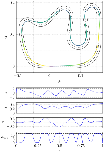
The example shown in Fig. 25 was obtained with the following numerical values: We use box priors on the corresponding model outputs to constrain the deviation from the centerline to $-0.006\leq z\leq 0.006$ with $\gamma_{z}=0.005$, the vehicle’s longitudinal acceleration to $-1\leq a\leq 1$ with $\gamma_{a}=0.001$, the steering angle to $-0.35\leq\delta\leq 0.35$ with $\gamma_{\delta}=0.001$, and the total acceleration to $0\leq a_{\text{tot}}^{2}\leq 150$ with $\gamma_{a_{\text{tot}}^{2}}=10^{-8}$, where $\psi=25$. The prior on the terminal state $X_{K,6}$ is zero-mean Gaussian with variance $\mathchoice{\overarrow@\arrowfill@\smallleftarrow\relbar\relbar\displaystyle{V}}{\overarrow@\arrowfill@\smallleftarrow\relbar\relbar\textstyle{V}}{\overarrow@\arrowfill@\smallleftarrow\relbar\relbar\scriptstyle{V}}{\overarrow@\arrowfill@\smallleftarrow\relbar\relbar\scriptscriptstyle{V}}_{\mspace{-3.0mu}X_{K,6}}=500$. The model inputs are unconstrained, which is approximated by a zero-mean Gaussian on every $U_{k}$ with large variance $\mathchoice{\overarrow@\arrowfill@\relbar\relbar\smallrightarrow\displaystyle{V}}{\overarrow@\arrowfill@\relbar\relbar\smallrightarrow\textstyle{V}}{\overarrow@\arrowfill@\relbar\relbar\smallrightarrow\scriptstyle{V}}{\overarrow@\arrowfill@\relbar\relbar\smallrightarrow\scriptscriptstyle{V}}_{\mspace{-3.0mu}U_{k}}=\operatorname{diag}\left(10^{8},10^{8}\right)$. Furthermore, $K=1000$ spatial samples are used.

The color of the resulting vehicle trajectory in Fig. 25 indicates the speed of the vehicle. Clearly, the vehicle needs to slow down before taking sharp turns in order to keep the total acceleration sufficiently low, i.e., to prevent slipping. The turning radius is further limited by the maximum steering angle of the vehicle.

VI Conclusion

NUV priors allow to incorporate non-Gaussian priors and constraints into linear Gaussian models without affecting their computational tractability. We proposed new NUV representations of half-space constraints, and we elaborated on recently proposed discretizing NUV priors. We then discussed the use of such NUV representations for model predictive control, with a variety of constraints on the input, the output, or the internal state of the controlled system. In such applications, the computations amount to iterations of Kalman-type forward-backward recursions, with a complexity (per iteration) that is linear in the planning horizon. In consequence, this approach can handle long planning horizons, which distinguishes it from the prior art. For nonconvex constraints, this approach has no claim to optimality, but it is empirically very effective.

The proposed approach was illustrated with a variety of exemplary control problems including flappy-bird control and minimal-time race track control. An application to a real-world industrial control problem is demonstrated in a companion paper [31].

Appendix A Proofs and Derivations

A-A Proof of Theorem III-A2

Assume, without loss of generality, that $a<b$. We first rewrite (23) as

$$\hat{x} = \operatorname*{argmax}_{x}\max_{\theta}p(\breve{y}\hskip 0.20004pt|\hskip 0.80002ptx)p(x,\theta)$$ (122)

$$= \operatorname*{argmax}_{x}p(\breve{y}\hskip 0.20004pt|\hskip 0.80002ptx)p(x)$$ (123)

$$= \operatorname*{argmin}_{x}-\log\!\left(p(\breve{y}\hskip 0.20004pt|\hskip 0.80002ptx)p(x)\right)$$ (124)

$$= \operatorname*{argmin}_{x}\frac{(x-\mu)^{2}}{2s^{2}}+\gamma|x-a|+\gamma|x-b|$$ (125)

$$\triangleq \operatorname*{argmin}_{x}\tilde{\kappa}(x).$$ (126)

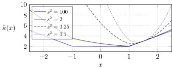
Maximizing (23) is thus equivalent to minimizing the cost function $\tilde{\kappa}(x)$, which is illustrated in Fig. 26, for different values of $s^{2}$.

Figure 26: Cost function $\tilde{\kappa}(x)$ in (126) for $a=-1,b=1,\mu=1.5,\gamma=1$, and different values for $s^{2}$. Condition (27) is satisfied for the solid lines, critically satisfied for the dashed line, and not satisfied for the dotted line.

Note that $\tilde{\kappa}(x)$ is a sum of convex functions and therefore also convex. Consequently, the estimate (122) is in the interval $[a,b]$ if and only if the global minimum of $\tilde{\kappa}(x)$ is in the interval $[a,b]$. This, in turn, is satisfied if and only if

$$\lim_{\tilde{x}\uparrow a}\left.\frac{\mathop{}\!\mathrm{d}\tilde{\kappa}(x)}{\mathop{}\!\mathrm{d}x}\right|_{x=\tilde{x}}<0\quad\text{and}\quad\lim_{\tilde{x}\downarrow b}\left.\frac{\mathop{}\!\mathrm{d}\tilde{\kappa}(x)}{\mathop{}\!\mathrm{d}x}\right|_{x=\tilde{x}}>0,$$ (127)

i.e.,

$$\frac{a-\mu}{s^{2}}-2\gamma<0\quad\text{and}\quad\frac{b-\mu}{s^{2}}+2\gamma>0,$$ (128)

which boils down to (27).

A-B Derivation of (44)

The derivation of ${{\hat{\sigma}_{a}}^{2}}$ in (44) is obtained by setting the derivative with respect to ${\sigma_{a}^{2}}$ of (43) to zero, i.e.,

$$\frac{\partial p(x,\theta)}{\partial{\sigma_{a}^{2}}} \stackrel{{\scriptstyle!}}{{=}} 0$$

$$\Leftrightarrow$$

$$({\sigma_{a}^{2}})^{-\frac{5}{2}}(x-a)^{2}-({\sigma_{a}^{2}})^{-\frac{3}{2}} \stackrel{{\scriptstyle!}}{{=}} 0$$ (130)

which yields the unique maximizer

$$({{\hat{\sigma}_{a}}^{2}})=\left(x-a\right)^{2}.$$ (131)

The maximizer ${{\hat{\sigma}_{b}}^{2}}$ in (44) is derived likewise.

A-C Derivation of (62) and (63)

The computation of $\big{(}{{\hat{\sigma}_{a}}^{2}}\big{)}^{(i)}$ follows from

$$\big{(}{{\hat{\sigma}_{a}}^{2}}\big{)}^{(i)} = \operatorname*{argmax}_{{\sigma_{a}^{2}}}\operatorname{\textnormal{$\mathbb{E}$}}\!\left[{\log\mathcal{N}\!\left({X;a,{\sigma_{a}^{2}}}\right)}\right]$$ (132)

$$= \operatorname*{argmin}_{{\sigma_{a}^{2}}}\left(\log({\sigma_{a}^{2}})+\frac{1}{{\sigma_{a}^{2}}}\operatorname{\textnormal{$\mathbb{E}$}}\!\left[{\left(X-a\right)^{2}}\right]\right)$$ (133)

$$= \operatorname{\textnormal{$\mathbb{E}$}}\!\left[{\left(X-a\right)^{2}}\right]$$ (134)

$$= \operatorname{\textnormal{$\mathbb{E}$}}\!\left[{X^{2}}\right]-\operatorname{\textnormal{$\mathbb{E}$}}\!\left[{X}\right]^{2}+\operatorname{\textnormal{$\mathbb{E}$}}\!\left[{X}\right]^{2}-2a\operatorname{\textnormal{$\mathbb{E}$}}\!\left[{X}\right]+a^{2}$$ (135)

$$= V_{X}^{(i)}+(\hat{x}^{(i)}-a)^{2},$$ (136)

where $\operatorname{\textnormal{$\mathbb{E}$}}\!\left[{X}\right]=\hat{x}^{(i)}$ was used. The step from (133) to (134) is obtained by setting the derivative with respect to ${\sigma_{a}^{2}}$ of (133) to zero. Likewise, we obtain

$$\big{(}{{\hat{\sigma}_{b}}^{2}}\big{)}^{(i)}=V_{X}^{(i)}+\big{(}\hat{x}^{(i)}-b\big{)}^{2}.$$ (137)

References

- [1] M. E. Tipping, “Sparse Bayesian learning and the relevance vector machine,” Journal of Machine Learning Research, vol. 1, pp. 211–244, 2001.
- [2] M. E. Tipping and A. C. Faul, “Fast marginal likelihood maximisation for sparse Bayesian models,” in Proc. of the Ninth International Workshop on Artificial Intelligence and Statistics, 2003, pp. 3–6.
- [3] D. P. Wipf and B. D. Rao, “Sparse Bayesian learning for basis selection,” IEEE Transactions on Signal Processing, vol. 52, no. 8, pp. 2153–2164, 2004.
- [4] D. P. Wipf and S. S. Nagarajan, “A new view of automatic relevance determination,” in Advances in Neural Information Processing Systems, 2008, pp. 1625–1632.
- [5] F. Bach, R. Jenatton, J. Mairal, and G. Obozinski, “Optimization with sparsity-inducing penalties,” Foundations and Trends in Machine Learning, vol. 4, no. 1, pp. 1–106, 2012.
- [6] I. Daubechies, R. DeVore, M. Fornasier, and C. S. Güntürk, “Iteratively reweighted least squares minimization for sparse recovery,” Communications on Pure and Applied Mathematics, vol. 63, no. 1, pp. 1–38, 2010.
- [7] H.-A. Loeliger, B. Ma, H. Malmberg, and F. Wadehn, “Factor graphs with NUV priors and iteratively reweighted descent for sparse least squares and more,” in Proc. Int. Symp. Turbo Codes & Iterative Inform. Process. (ISTC), 2018, pp. 1–5.
- [8] H.-A. Loeliger, L. Bruderer, H. Malmberg, F. Wadehn, and N. Zalmai, “On sparsity by NUV-EM, Gaussian message passing, and Kalman smoothing,” 2016, Information Theory and Applications Workshop (ITA), La Jolla, CA.
- [9] N. Zalmai, R. Keusch, H. Malmberg, and H.-A. Loeliger, “Unsupervised feature extraction, signal labeling, and blind signal separation in a state space world,” in Poc. 25th European Signal Processing Conference (EUSIPCO), 2017, pp. 838–842.
- [10] N. Zalmai, H. Malmberg, and H.-A. Loeliger, “Blind deconvolution of sparse but filtered pulses with linear state space models,” in Proc. IEEE Int. Conf. on Acoustics, Speech and Signal Processing (ICASSP), 2016, pp. 4194–4198.
- [11] N. Zalmai, “A State Space World for Detecting and Estimating Events and Learning Sparse Signal Decompositions,” Ph.D. dissertation, ETH Zurich, 2017.
- [12] F. Wadehn, T. Weber, D. J. Mack, T. Heldt, and H.-A. Loeliger, “Model-based separation, detection, and classification of eye movements,” IEEE Transactions on Biomedical Engineering, vol. 67, no. 2, pp. 588–600, Feb. 2020.
- [13] F. Wadehn, L. Bruderer, J. Dauwels, V. Sahdeva, H. Yu, and H.-A. Loeliger, “Outlier-insensitive Kalman smoothing and marginal message passing,” in Proc. 24th European Signal Processing Conference (EUSIPCO), Budapest, Hungary, Aug. 2016, pp. 1242–1246.
- [14] F. Wadehn, “State Space Methods With Applications in Biomedical Signal Processing,” Ph.D. dissertation, No. 25926, ETH Zurich, 2019.
- [15] L. Bruderer, “Input Estimation And Dynamical System Identification: New Algorithms and Results,” Ph.D. dissertation, No. 22575, ETH Zurich, 2015.
- [16] C. Hoffmann and P. Rostalski, “Linear optimal control on factor graphs – a message passing perspective,” in Proc. of the 20th IFAC World Congress, 2017.
- [17] B. Ma, J. Trisovic, and H.-A. Loeliger, “Multi-image blind deblurring using a smoothed NUV prior and iteratively reweighted coordinate descent,” in Proc. IEEE International Conference on Image Processing (ICIP), 2020, pp. 973–977.
- [18] B. Ma, N. Zalmai, and H.-A. Loeliger, “Smoothed-NUV priors for imaging,” IEEE Transactions on Image Processing, pp. 4663–4678, 2022.
- [19] R. Keusch, H. Malmberg, and H.-A. Loeliger, “Binary control and digital-to-analog conversion using composite NUV priors and iterative Gaussian message passing,” in Proc. IEEE Int. Conf. on Acoustics, Speech and Signal Processing (ICASSP), 2021, pp. 5330–5334.
- [20] G. Marti, R. Keusch, and H.-A. Loeliger, “Multiuser MIMO detection with composite NUV priors,” 2021, international Symposium on Topics in Coding (ISTC).
- [21] R. Keusch and H.-A. Loeliger, “A binarizing NUV prior and its use for M-level control and digital-to-analog conversion,” arXiv: 2105.02599, 2021.
- [22] ——, “Half-space and box constraints as NUV priors: First results,” 2021, arXiv: 2109.00036, 2021.
- [23] D. P. Bertsekas, “Projected Newton methods for optimization problems with simple constraints,” SIAM Journal on Control and Optimization, vol. 20, no. 2, pp. 221–246, 1982.
- [24] D. Kim, S. Sra, and I. S. Dhillon, “Tackling box-constrained optimization via a new projected quasi-Newton approach,” SIAM Journal on Scientific Computing, vol. 32, no. 6, pp. 3548–3563, 2010.
- [25] J. B. Rosen, “The gradient projection method for nonlinear programming. Part I. Linear constraints,” Journal of the Society for Industrial and Applied Mathematics, vol. 8, no. 1, pp. 181–217, 1960.
- [26] S. J. Wright, Primal-Dual Interior-Point Methods. Philadelphia: SIAM, 1997.
- [27] P. B. Stark and R. L. Parker, “Bounded-variable least-squares: an algorithm and applications,” Computational Statistics, vol. 10, pp. 129–129, 1995.
- [28] E. J. Fuentes, C. Silva, D. E. Quevedo, and E. I. Silva, “Predictive speed control of a synchronous permanent magnet motor,” Churchill, VIC, Australia, Feb. 2009.
- [29] B. Hassibi and H. Vikalo, “On the sphere-decoding algorithm: I. Expected complexity,” IEEE Transactions on Signal Processing, vol. 53, no. 8, pp. 2806–2818, 2005.
- [30] P. Karamanakos, T. Geyer, and R. Kennel, “Constrained long-horizon direct model predictive control for power electronics,” Milwaukee, WI, USA, Sep. 2016.
- [31] R. Keusch and H.-A. Loeliger, “Long-horizon direct model predictive control for power converters with state constraints,” submitted to IEEE Transactions on Control Systems Technology, September 2022.
- [32] R. Tibshirani, “Regression shrinkage and selection via the LASSO,” Journal of the Royal Statistical Society: Series B (Methodological), vol. 58, no. 1, pp. 267–288, 1996.
- [33] M. Nagahara, “Discrete signal reconstruction by sum of absolute values,” IEEE Signal Processing Letters, vol. 22, no. 10, pp. 1575–1579, 2015.
- [34] P. Bromiley, “Products and convolutions of Gaussian probability density functions,” Tina-Vision Memo, vol. 3, no. 4, p. 1, 2003.
- [35] H.-A. Loeliger, “An introduction to factor graphs,” IEEE Signal Processing Magazine, vol. 21, no. 1, pp. 28–41, 2004.
- [36] R. Giri and B. Rao, “Type I and type II Bayesian methods for sparse signal recovery using scale mixtures,” IEEE Transactions on Signal Processing, vol. 64, no. 13, pp. 3418–3428, 2016.
- [37] P. Stoica and Y. Selén, “Cyclic minimizers, majorization techniques, and the expectation-maximization algorithm: a refresher,” IEEE Signal Proc. Mag., vol. 21, no. 1, pp. 112–114, 2004.
- [38] M. Frey and H.-A. Loeliger, “On the static resolution of digitally-corrected analog-to-digital and digital-to-analog converters with low-precision components,” IEEE Trans. Circuits & Systems I, vol. 54, no. 1, pp. 229–237, 2007.
- [39] G. J. Bierman, Factorization Methods for Discrete Sequential Estimation. New York: Academic Press, 1977.
- [40] C. Hoffmann, A. Isler, and P. Rostalski, “A factor graph approach to parameter identification for affine LPV systems,” in American Control Conference (ACC), 2017, pp. 1910–1915.
- [41] “Flappy bird,” https://en.wikipedia.org/wiki/Flappy_Bird.
- [42] X. Qian, A. de La Fortelle, and F. Moutarde, “A hierarchical model predictive control framework for on-road formation control of autonomous vehicles,” in Proc. IEEE Intelligent Vehicles Symposium (IV), Jun. 2016, pp. 376–381.
- [43] X. Qian, “Model Predictive Control for Autonomous and Cooperative Driving,” Ph.D. dissertation, PSL Research University, 2016.
- [44] U. Rosolia and F. Borrelli, “Learning how to autonomously race a car: a predictive control approach,” arXiv: 1901.08184, 2019.
- [45] R. Lot and F. Biral, “A curvilinear abscissa approach for the lap time optimization of racing vehicles,” IFAC Proceedings Volumes, vol. 47, no. 3, pp. 7559–7565, Jan. 2014.
- [46] A. Micaelli and C. Samson, “Trajectory tracking for unicycle-type and two-steering-wheels mobile robots,” Research Report RR-2097, 1993.
- [47] R. Lenain, B. Thuilot, C. Cariou, and P. Martinet, “Adaptive and predictive path tracking control for off-road mobile robots,” European Journal of Control, vol. 13, pp. 419–439, Jul. 2007.
- [48] ——, “Advanced path tracking control for off-road mobile robots,” in Workshop on Modeling, Estimation, Path Planning and Control of All Terrain Mobile Robots, 2008, pp. 32–40.
- [49] R. Rajamani, Vehicle Dynamics and Ccontrol. Berlin/Heidelberg: Springer Science & Business Media, 2011.