Towards robust corrections for stellar contamination in JWST exoplanet transmission spectra

Abstract

Transmission spectroscopy is still the preferred characterization technique for exoplanet atmospheres, although it presents unique challenges which translate into characterization bottlenecks when robust mitigation strategies are missing. Stellar contamination is one of such challenges that can overpower the planetary signal by up to an order of magnitude, and thus not accounting for stellar contamination can lead to significant biases in the derived atmospheric properties. Yet, accounting for stellar contamination may not be straightforward, as important discrepancies exist between state-of-the-art stellar models and measured spectra and between models themselves. Here we explore the extent to which stellar models can be used to reliably correct for stellar contamination and yield a planet’s uncontaminated transmission spectrum. We find that (1) discrepancies between stellar models can dominate the noise budget of JWST transmission spectra of planets around stars with heterogeneous photospheres; (2) the true number of unique photospheric spectral components and their properties can only be accurately retrieved when the stellar models have a sufficient fidelity; and (3) under such optimistic circumstances the contribution of stellar contamination to the noise budget of a transmission spectrum is considerably below that of the photon noise for the standard transit observation setup. Therefore, we suggest (1) increased efforts towards development of model spectra of stars and their active regions in a data-driven manner; and (2) the development of empirical approaches for deriving spectra of photospheric components using the observatories with which the atmospheric explorations are carried out.

1 Introduction

Transmission spectroscopy, the multiwavelength study of the shadows cast by transiting exoplanets (e.g., Seager & Sasselov, 2000; Brown, 2001), provides a powerful tool for constraining the physical structure and chemical composition of exoplanet atmospheres, as recently demonstrated by the JWST Early Release Science observations of WASP-39b (JWST Transiting Exoplanet Community Early Release Science Team et al., 2023; Ahrer et al., 2023; Alderson et al., 2023; Feinstein et al., 2023; Rustamkulov et al., 2023). However, the transmission spectrum only contains information related to the wavelength-dependent opacity of a planet’s atmosphere alone when the stellar disk is limb darkened but otherwise featureless. For stars with notable coverage of photospheric heterogeneities like spots and faculae, the difference in the hemisphere-averaged emission spectrum of the star and the transit-chord-averaged one imprints features in the transmission spectrum (e.g., Sing et al., 2011; McCullough et al., 2014), a phenomenon dubbed the transit light source (TLS) effect (Rackham et al., 2018, 2019). Active FGK stars and nearly all M dwarfs are expected to produce detectable TLS, or “stellar contamination,” signals in precise transmission spectra (Rackham et al., 2018, 2019).

Given this context, recent work has sought to constrain and mitigate for the heterogeneity of the stellar disk at the time of transit by leveraging the stellar spectrum collected during the out-of-transit baseline. Specifically, the temperatures and filling factors of the different photospheric components are constrained to later correct for their contributions to the joint in-transit spectrum (e.g., Zhang et al., 2018; Wakeford et al., 2019; Garcia et al., 2022). Early on, these mitigation studies revealed two bottlenecks. First, fitting host-star spectra with the precisions afforded by space-based platforms is a challenge for current models, especially for late-M dwarfs such as TRAPPIST-1 (Gillon et al., 2016, 2017). Zhang et al. (2018) showed that the uncertainties on the HST/WFC3/G141 spectra of TRAPPIST-1 need to be inflated by factors of $\sim$23 to produce adequate fits with respect to stellar models. The subsequent studies of Wakeford et al. (2019) and (Garcia et al., 2022) yielded consistent challenges, which are expected to worsen in the JWST era following a substantial increase in precision (see recent review from Rackham et al., 2022). Second, with the current data quality and model fidelity, an ensemble of models may fit an out-of-transit spectrum equally well, leading to a range of corrected atmospheric spectra with a scatter many times larger than the photon noise (see, e.g., Fig. 6 from Wakeford et al. 2019 and Fig. 7 from Garcia et al. 2022).

As stellar contamination can overpower the planetary signal by up to an order of magnitude (Rackham et al., 2018), not accounting for it when performing atmospheric retrieval can lead to important biases in inferred planetary atmospheric parameters (Iyer & Line, 2020). A zeroth-order mitigation strategy to account for the imperfections of stellar models and avoid biases in the corrected planetary spectra is thus to inflate the uncertainties of the stellar spectra (e.g., Zhang et al., 2018), thereby decreasing the precision of planetary inferences. However, the optimal study of exoplanet atmospheres with current facilities demands refined mitigation approaches that can harness the precision of these observations to reduce biases and uncertainties as much as possible.

Here we explore the limits of using baseline out-of-transit observations to infer the photospheric properties of cool stars and mitigate for stellar contamination in transmission spectra, with a particular consideration for the fidelity of current stellar models. Our analysis complements that recently conducted for opacity models by Niraula et al. (2022, hereafter N22). Finally, we evaluate how the contribution of the stellar contamination to the noise budget scales with the ratio out- vs in-transit of observations. We first investigate the utility of out-of-transit JWST spectra for identifying a complex photosphere with multiple spectral components and whether inferences are limited by the data quality at hand or the fidelity of stellar spectral models. If the later, this means that new stellar models (theoretical or empirical) may help us move towards a photon-noise-dominated regime. Then, setting aside model fidelity, we assess whether this approach permits inferences of photospheric parameters that are accurate and precise enough to reduce biases in transmission spectra. Finally, we evaluate the contribution of stellar contamination to the total noise and how this scales with the ratio of the out-of-transit to in-transit observations. Note that we focus in this paper on configurations in which heterogeneities are present but not occulted by the transiting exoplanet. Mitigation strategies for occulted active regions can be found in other studies (e.g., Fu et al., 2022).

This paper is organized as follows. Section 2 presents our approach for generating the synthetic datasets for analysis. Section 3 details our retrieval approach for inferring constraints from simulated out-of-transit stellar spectra. Section 4 shares our results, and Section 5 summarizes our findings while placing them in the larger context of JWST observations.

2 Data synthesis

In order to explore the ability of current stellar models to support the reliable correction of stellar contamination in JWST exoplanet transmission spectra, we follow a sensitivity analysis similar to that introduced in N22 for opacity models. We explore two systems and five level of heterogeneities in our sensitivity analysis, which we describe in the following section.

2.1 Properties of the Synthetic Systems

We adopt synthetic systems similar to those introduced in N22 as representative examples of planets that would be high-priority targets for JWST. These correspond to an Earth-sized planet around a M-dwarf star and a Jupiter-sized planet around a K-dwarf star.

The warm Jupiter has a mass of $1\,M_{\mathrm{jup}}$, radius of $1\,R_{\mathrm{jup}}$, a reference temperature of 500 K, and a transit duration of 5.80 hr. The super Earth has a mass of $1\,M_{\mathrm{\earth}}$, radius of $1\,R_{\mathrm{\earth}}$, a reference temperature of 300 K, and a transit duration of 1.00 hr. The details of the atmospheric model of each planet, given in Table 2 of N22, are not important for this analysis, as we are interested instead in the impact of the host stars.

The K dwarf has an effective temperature of $T_{\mathrm{eff}}=5270$ K, a stellar mass of $M_{s}=0.88\,M_{\sun}$, and a stellar radius of $R_{s}=0.813\,R_{\sun}$, parameters which correspond to a K0 dwarf (Pecaut & Mamajek, 2013). For the M dwarf, $T_{\mathrm{eff}}=2810\,K$, $M_{s}=0.102\,M_{\sun}$, and $R_{s}=0.137\,R_{\sun}$, corresponding to an M6 dwarf (Pecaut & Mamajek, 2013). In both cases, we consider solar metallicity stars ($\mathrm{[Fe/H]}=0.0$). We also adopt a brightness of $J=11$ for both host stars, giving distances of 191 pc and 20.5 pc for the K0 and M6 stars, respectively.

2.2 Synthetic Cases of Photospheric Heterogeneity

For each host star, we consider five photospheric heterogeneity scenarios, detailed in Table 1. The first case, case 1, is a quiescent star, for which the quiescent-photosphere spectrum is the only spectral component present on the stellar disk. The next two cases, case 2l and case 2h, are for a star with two spectral components, those of the quiescent photosphere and a spot. The spot coverage is 1% in the low-activity case (case 2l) and 5% in the high-activity case (case 2h). The last two cases, case 3l and case 3h, are for a star with three spectral components, those of the quiescent photosphere, spots, and faculae. The coverages of the spots are the same as the previous low-activity and high-activity cases, and the coverages of the faculae are 10% and 30% for case 3l and case 3h, respectively.

1	no activity	0	0
2l	spots, low activity	1	0
2h	spots, high activity	5	0
3l	spots and faculae, low activity	1	10
3h	spots and faculae, high activity	5	30

Table 1: Parameters of the five heterogeneity cases.

For each star, we adopt the effective temperature as the temperature of the quiescent photosphere. For the K dwarf, we set the spot and facula temperatures to 3830 K and 5380 K, respectively, following Rackham et al. (2019). For the M dwarf, we set the spot temperature to 86% of the photospheric temperature (2420 K) and the facula temperature to 2910 K, following Afram & Berdyugina (2015) and Rackham et al. (2018), respectively.

We generate the model truth of the (out-of-transit) stellar spectrum as the linear combination of the constituent spectra weighted by their filling factors. We do not assume any specific position on the stellar disk for the spots and faculae besides that they are present outside of the transit chord and thus undetectable via crossing events (e.g., Fu et al., 2022). As a result, we take the component spectra to be representative of spots at all positions and neglect the impact of limb darkening.

2.3 Stellar Spectral Models

We perform what we call “direct” and “cross” retrievals to explore the impact of imperfections in the stellar spectral models on our inferences. In both cases, the synthetic data are generated using the PHOENIX stellar spectral model grid (Husser et al., 2013). Relevant to our purposes, the PHOENIX grid spans effective temperatures of $T_{\mathrm{eff}}\in[2300,7000]$ K in 100 K steps and surface gravities of $\log g\in[0.0,6.0]$ in steps of 0.5. For all spectral models, we linearly interpolate between grid points in terms of $T_{\mathrm{eff}}$, $\mathrm{[Fe/H]}$, and $\log g$ using the speclib package.

For the cross retrievals, we use other model grids to retrieve on the data. This allows us to examine potential limitations introduced by the models under the assumption that the differences between state-of-the-art models provide a proxy of the differences between the models and reality. At the sampling of our simulated datasets (see Section 2.4), these differences average ${\sim}10$ ppt for K0 stars and earlier types and ${\sim}200$ ppt for M6 stars—with local differences above 100% (Figure 1). Considering that planetary signals within reach of JWST’s precision can be of the order of a few hundred parts per million (e.g., Rustamkulov et al., 2023), it is crucial to explore how uncertainties stemming from model fidelity will challenge our retrievals that incorporate TLS signals.

Due to the different temperature regimes of the state-of-the-art model grids, we used different models for the K0 and M6 cross retrievals. For the K0 case, we used the MPS-ATLAS model grid (Witzke et al., 2021; Kostogryz et al., 2023). This grid spans effective temperatures of $T_{\mathrm{eff}}\in[3500,9000]$ K in 100 K steps and surface gravities of $\log g\in\{3.0,3.5,4.0,4.2,4.3,4.4,4.5,4.6,4.7,5.0\}$. For the M6 case, we used the SPHINX model grid (Iyer et al., 2023). This grid spans effective temperatures of $T_{\mathrm{eff}}\in[2000,4000]$ K in 100 K steps and surface gravities of $\log g\in[4.0,5.5]$ in steps of 0.25. As with the direct retrievals, we fixed the metallicity ([Fe/H] or [M/H]) of all spectra to 0. For the SPHINX model grid, we also fixed $\mathrm{C/O}=0.5$.

Figure 1: State-of-the-art model spectra of quiescent K0 and M6 dwarfs at the wavelengths and resolution of NIRSpec/PRISM. The left column shows spectra of a K0 dwarf drawn from the PHOENIX and MPS-ATLAS grids. The top panel shows the spectra, and the bottom panel shows the flux difference between them, normalized to the flux of the PHOENIX model. The right column shows the same for the PHOENIX and SPHINX spectra of the M6 dwarf used as an example in this work. Note that PHOENIX and MPS-ATLAS spectra span the full wavelength range of NIRSpec/PRISM, though SPHINX spectra have a long-wavelength limit of $3\,\micron$. See also Iyer et al. (2023, Fig. 1) for a comparison of M-dwarf spectra across many stellar models.

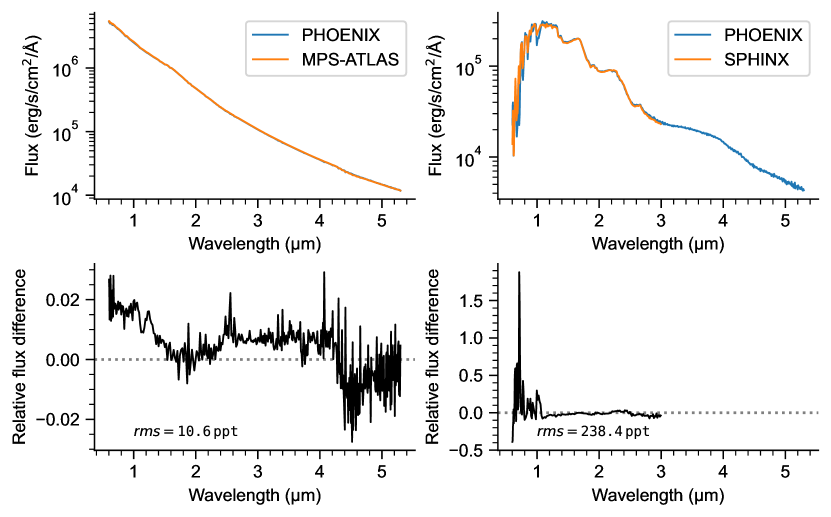
All three model grids—PHOENIX, MPS-ATLAS, and SPHINX—are calculated at higher spectral resolutions than provided by NIRSpec/PRISM ($R{\sim}100$), the instrument for our simulated observations (see Section 2.4), so we downsampled the spectra to match the wavelengths and resolution of the data. While the wavelength range of the PHOENIX and MPS-ATLAS models span the 0.6–5.3 $\micron$ range of NIRSpec/PRISM, we note that the SPHINX spectra have a long-wavelength limit of 3 $\micron$. We discuss the impact of this on our analysis in Section 3.4.

2.4 Simulated precisions

Table 2: Free parameters and their priors for the four retrieval models.

1-comp	$\mathcal{U}(2300,5500)$	…	…	…	$\mathcal{U}(0.08,1.00)$	$\mathcal{U}(-50,0)$
2-comp	$\mathcal{U}(2300,5500)$	$\mathcal{U}(1/2,1)$	…	…	$\mathcal{U}(0.08,1.00)$	$\mathcal{U}(-50,0)$
3-comp	$\mathcal{U}(2300,5500)$	$\mathcal{U}(1/3,1)$	$\mathcal{U}(1/2,1)$	…	$\mathcal{U}(0.08,1.00)$	$\mathcal{U}(-50,0)$
4-comp	$\mathcal{U}(2300,5500)$	$\mathcal{U}(1/4,1)$	$\mathcal{U}(1/3,1)$	$\mathcal{U}(1/2,1)$	$\mathcal{U}(0.08,1.00)$	$\mathcal{U}(-50,0)$

Note. — $\mathcal{U}(a,b)$ designates a uniform prior over the range $(a,b)$.

We simulated the precision of JWST observations of our synthetic targets using PandExo (Batalha et al., 2017). We focus on observations with the Near Infrared Spectrograph (NIRSpec) with the low-resolution ($R{\sim}100$) PRISM disperser, following the approach of the observations of WASP-39b (JWST Transiting Exoplanet Community Early Release Science Team et al., 2023; Rustamkulov et al., 2023) through the JWST Transiting Exoplanet Community Early Release Science Program (Bean et al., 2018). At higher resolutions, such as those available with NIRSpec’s gratings and NIRISS SOSS, we expect that both the impact of stellar contamination and the precision of the associated inferences will be increased owing to a higher information content. NIRSpec/PRISM thus provides a good case to explore our interest in the limitations of out-of-transit inferences for a common JWST transit observation mode.

We used NIRSpec in Bright Object Time Series mode with the $1\farcs 6\times 1\farcs 6$ fixed-slit aperture (s1600a1) and PRISM disperser. This setup provides spectra spanning 0.6–5.3 $\micron$ at a spectral resolving power of $R{\sim}100$. We also used the SUB512 subarray, five groups per integration, and the NRSRAPID read mode. We set the total observing time to three times the transit duration. We assumed a constant noise floor of 10 ppm, consistent with the $3\sigma$ upper limit of 14 ppm measured in lab time series (Rustamkulov et al., 2022) and the lack of significant systematic errors noted in the observations of WASP-39b (Rustamkulov et al., 2023). We note that our choice of $J{=}11$ apparent magnitudes for the host stars places them among the best targets that can be observed with NIRSpec/PRISM, making our simulated datasets among the best single-visit datasets possible with this observing mode. Combining the data from the full out-of-transit baseline, our simulated spectra have a typical per-pixel signal-to-noise ratio (SNR) of 16 000 (${\sim}$62 ppm error).

3 Retrievals

We retrieved on each of the 10 simulated out-of-transit stellar spectra (2 host stars $\times$ 5 activity levels) using four models, accounting for one, two, three, and four spectral components, respectively. We refer to these as the “1-comp,” “2-comp,” “3-comp”, and “4-comp” models hereafter. The rationale behind testing this range of model complexity is that it encompasses all of the true complexity of our input models and more, thereby allowing us to assess when biases emerge from our inability to robustly constrain the true complexity of the observed photosphere. The following section provides further details on the models and the retrieval procedure.

3.1 Model Definition

We model the flux at wavelength $\lambda$ received from each host star $F_{\lambda}$ as

$$F_{\lambda}=\sum_{i=1}^{N}f_{i}S_{i,\lambda}\left(\frac{R_{s}}{D_{s}}\right)^{2},$$ (1)

in which $f_{i}$ and $S_{i,\lambda}$ are the filling factors and emergent spectra of the $i$th spectral component present on the stellar disk, $N$ is the number of spectral components, $R_{s}$ is the stellar radius, and $D_{s}$ is the stellar distance. The units of our model and simulated data are erg s^-1 cm^-2 Å^-1.

The goal of the retrieval procedure is to identify the values that maximize the likelihood $\mathcal{L}$ of the model ($F_{\mathrm{model}}$) when compared to the data ($F_{\mathrm{data}}$). For the natural logarithm of the likelihood function, we adopt

$$\log\mathcal{L}=-\frac{1}{2}\sum\left(\frac{(F_{\mathrm{data,\lambda}}-F_{\mathrm{model,\lambda}})^{2}}{\sigma_{\lambda}^{2}}+\log\left(2\pi\sigma_{\lambda}^{2}\right)\right).$$ (2)

Following Foreman-Mackey et al. (2013, 2019), we model the $\sigma_{\lambda}$ as the quadrature sum of photon noise $\sigma_{\mathrm{phot,\lambda}}$, given by the simulations in Section 2.4, and an additional noise term $\sigma_{\mathrm{jitter,\lambda}}$, which encapsulates any additional noise present in the data. We parameterize the additional noise as a fractional underestimation of the variance following

$$\sigma_{\mathrm{jitter,\lambda}}=f_{\mathrm{var}}F_{\mathrm{model,\lambda}},$$ (3)

which means that the amplitude of $\sigma_{\mathrm{jitter,\lambda}}$ scales with the model flux. While we did not inject systematic noise into the simulations, this approach adds a level of realism to our retrievals, effectively inflating the data uncertainty to account for any shortcomings of our models in describing the data.

3.2 Priors

Table 2 summarizes the free parameters for our four models and their priors. We parameterize the spectral components by their temperatures ($T_{1}$, $T_{2}$ $T_{3}$, and $T_{4}$), and we place wide, uniform priors on all temperatures. To prevent degenerate solutions and automatically ensure the number order of the components corresponds to their prevalence on the stellar disk, we fit for their filling factors using a set of ratio parameters ($r_{1}$, $r_{2}$, and $r_{3}$) with specific priors. In brief, the ratio parameters describe the ratio of the stellar disk filled by the component of interest relative to less prevalent spectral components. Thus, a model with $N$ spectral components will include $N-1$ ratio parameters. For example, in the 1-comp model we do not need to fit for any filling factors ($f_{1}=1$, by definition), and so we do not fit for any ratio parameters. By contrast, in the 4-comp model we need to fit for four filling factors ($f_{1}$, $f_{2}$, $f_{3}$, and $f_{4}$), and so we do that using three ratio parameters ($r_{1}$, $r_{2}$, and $r_{3}$).

Mathematically, we define each $n$th ratio parameter as

$$r_{n}=\frac{f_{n}}{\sum_{i=n}^{N}f_{i}},$$ (4)

in which $N$ is again the total number of components. We place a uniform prior $\mathcal{U}_{n}(a,b)$ on each $n$th ratio parameter defined by $a=1/(N+1-n)$ and $b=1$. Importantly, the definitions of $r_{n}$ and $\mathcal{U}_{n}$ depend on $N$ and this differ between models. For example, as shown in Table 2, in the 3-comp model $r_{2}=f_{2}/(f_{2}+f_{3})$ and its prior is $\mathcal{U}_{2}(1/2,1)$, whereas in the 4-comp model $r_{2}=f_{2}/(f_{2}+f_{3}+f_{4})$ and its prior is $\mathcal{U}_{2}(1/3,1)$. In any case, for the models in which they are defined, the filling factors $f_{1}$ to $f_{4}$ can be calculated as

$$f_{1}=r_{1},$$ (5a)

$$f_{2}=(1-r_{1})r_{2},$$ (5b)

$$f_{3}=(1-r_{1})(1-r_{2})r_{3},$$ (5c)

and

$$f_{4}=(1-r_{1})(1-r_{2})(1-r_{3})r_{4},$$ (5d)

by setting $r_{i}=1$ for $i\geq N$.

The stellar radius and distance are fully degenerate parameters in our model (Equation 1). Rather than assuming errors to use for normal priors on these parameters, we fix $D_{s}$ to the adopted distance and fit for $R_{s}$ with a uniform prior. We also fix the stellar metallicity [Fe/H] to 0 and the surface gravity $\log g$ to the value given by the mass and radius of host star provided in Section 2.1.

The final free parameter in each model is the fractional underestimation of the variance $f_{\mathrm{var}}$, which accounts for additional noise in the data (Equation 3). To ensure it is always positive and to allow the sampling to explore a large dynamic range, we actually fit for $\log f_{\mathrm{var}}$ with a uniform prior of $(-50,0)$. We note that the median value of $\log(\sigma_{\mathrm{phot,\lambda}}/F_{\mathrm{data,\lambda}})$ is $-10$, and so the parameter space included in this prior spans scenarios in which systematic errors are many orders of magnitude below or above the photon noise.

In total, there are three, five, seven, and nine free parameters for the 1-comp, 2-comp, 3-comp, and 4-comp models, respectively.

3.3 Model Inference

We derive the posterior probability distributions of the model parameters with the nested sampling Monte Carlo algorithm MLFriends (Buchner, 2014, 2017) using the UltraNest Python package (Buchner, 2021). We use slice sampling to efficiently explore the parameter space, defining the number of steps as 10 times the number of parameters and setting the maximum number of improvement loops to 3 to limit computational runtimes without appreciably affecting the posterior inferences. At each sampling step, we use the speclib Python package to generate the component spectra included in the model. We use the SpectralGrid object within speclib to do this efficiently, loading a spectral grid into memory once with the fixed metallicity and surface gravity values and linearly interpolating between temperature grid points to produce the sample spectra. We note that linear interpolation is likely not the best approach in the high signal-to-noise regime in which we are operating here. We discuss this complication further in Section 5.

3.4 Model Selection

Our studied parameter space covers 10 simulated datasets (2 host stars $\times$ 5 activity levels). We retrieve on each using two spectral grids, the PHOENIX grid or another (MPS-ATLAS or SPHINX). For each dataset–grid pair, we would like to test our four model complexities (1-comp to 4-comp) and determine which model best describes the data.

We do this with UltraNest by computing the Bayesian evidence ($\log\mathcal{Z}$) of each model, which we use as the basis for model selection. We define the best model as the simplest model that produces a significantly better fit than other models. We adopt a Bayes factor of $\Delta\log\mathcal{Z}=5.0$ as the threshold for significance, corresponding to an odds ratio of ${\sim}150:1$ (Trotta, 2008) or a $3.6\sigma$ result (Benneke & Seager, 2013). In other words, we selected a more complex model over a simpler one only when it provides a marginal increase in the $\log\mathcal{Z}$ of 5.0 or more.

The SPHINX spectra have a long-wavelength end of $3\,\micron$. Thus, to fairly compare evidences, we perform retrievals of the M6 spectra with the PHOENIX and SPHINX grids using datasets truncated at $3\,\micron$. These are in addition to direct retrievals of the full datasets using the PHOENIX grid.

In total, the nested-sampling retrievals in this analysis cover 2 host stars, 5 activity levels, 2 spectral model grids, and 4 model complexities.

Figure 2: Bayesian evidences for model fits with different levels of complexity in the case of the direct retrievals. Here the same model grid was used to simulate and retrieve on the data. The top row gives results for the K0 star. The bottom row gives results for the M6 star. From left to right, the columns gives results for the 1, 2l, 2h, 3l, and 3h cases, respectively. In each panel, the marginal Bayesian evidence for the 1-, 2-, 3-, and 4-component models are shown. The marginal Bayesian evidence is defined relative to the selected model, with more positive values indicating a higher preference. Triangles point to evidences that fall below the limit of the y-axis, indicating that model is a relatively poor fit to the the data (${>}5\sigma$ preference against). The shaded regions highlight the appropriate complexity for a dataset; they are green if the inferred complexity is correct and red if not. In all but one case, the direct retrieval (i.e., model fidelity) identify the correct complexity.

4 Results

In analyzing the results of the retreivals, we focus on three topics: whether we can infer the correct level of complexity, whether we can retrieve the correct input parameters and thus reduce biases, and the impact of accounting for the heterogeneity on the uncertainty budget. We present each of these topics in turn in the following section.

4.1 Inferring the Correct Level of Complexity

Figure 3: Bayesian evidences for model fits with different levels of complexity in the case of the cross retrievals. The figure elements are the same as those of Figure 3. The top row gives results for the K0 star, simulated with PHOENIX and retrieved with MPS-ATLAS. The bottom row gives results for the M6 star, simulated with PHOENIX and retrieved with SPHINX. In most cases, the cross retrievals (i.e., no model fidelity) fail to identify the correct complexity.

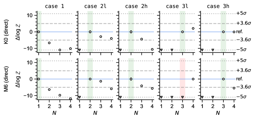
We start by reviewing the results for the direct-retrieval cases, which assume model fidelity. As detailed in Section 3.4, we analyzed 10 simulated spectra, trying to fit to each four models with varying levels of complexity. We find that the correct level of complexity was inferred in nine out of 10 cases (Figure 2). In other words, in nearly all cases the model with the appropriate number of components provided a large enough increase in $\log\mathcal{Z}$ to warrant its use and more complex models were not warranted. As a result, in nearly all cases, retrieving the right level of complexity enabled unbiased inferences on the heterogeneity properties and the optimal correction of the stellar contamination. In the full set of direct retrievals, the median standard deviations of the inferred temperatures and filling factors were 2 K and 0.6%, respectively.

The exception to this pattern was the M6 case 3l dataset. In this case, the 4-comp model gave a fit that improved the Bayesian evidence by $\Delta\log\mathcal{Z}=57.5$ with respect to the (appropriate) 3-comp model. This indicates a preference for the more complicated model that is much greater than our $3.6\sigma$ significance threshold or even the more rigorous threshold of $\Delta\log\mathcal{Z}=11$, corresponding to an odds ratio of $43000:1$ or a $5\sigma$ result (Benneke & Seager, 2013). Inspecting the results of the 3-comp and 4-comp retrievals shows that the inclusion of the fourth component gives the algorithm flexibility to compensate for the particular noise instance, allowing for a lower posterior constraint on $\log f_{\mathrm{var}}$ and thus a higher Bayesian evidence. We discuss the practical impact of this mislabeling of the M6 case 3l dataset in terms of the ultimate correction applied to the transmission spectrum in Section 4.2.

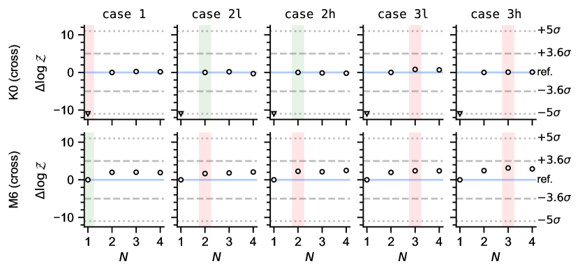
We now turn to the results of the cross-retrieval cases. Here the results are similar for all cases of a given host star (Figure 3). In each K0 case, the MPS-ATLAS retrievals indicate a preference for the 2-comp model when compared to other MPS-ATLAS models. Similarly, in each M6 case, the SPHINX retrievals find the 1-comp model to be best. As a result, the K0 and M6 retrievals infer the correct level of complexity in 2/5 and 1/5 cases, respectively. For the MPS-ATLAS cross retrievals, the median standard deviations of the inferred temperatures and filling factors were 39 K and 0.8%, respectively. For the SPHINX cross retrievals, the median standard deviations of the inferred temperatures was 21 K and the selected models had no filling factors to fit.

Nonetheless, whether the cross retrievals happened to identify the right level of complexity or not, they universally provide poor fits to the data in this high signal-to-noise regime. When compared to the results of the PHOENIX retrievals for the same case (and wavelength range, for the PHOENIX–SPHINX comparison), all cross-retrieval models are strongly disfavored at ${\gg}5\sigma$. Typical values of $\Delta\log\mathcal{Z}$ are ${\sim}10^{4}$ in favor of the PHOENIX models. In terms of reduced chi-square values, PHOENIX model fits have $\chi^{2}_{r}\sim 1$ before accounting for the inflated uncertainties, while the corresponding values for the cross-retrievals are $\chi^{2}_{r}\sim 10^{4}$ for the MPS-ATLAS models and $\chi^{2}_{r}\sim 10^{6}$ for the SPHINX models.

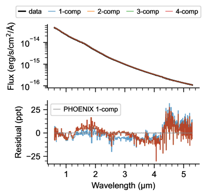
As an example, we highlight the K0 case 1 cross-retrieval with the MPS-ATLAS grid (Figure 4). Like our other simulated spectra, this spectrum has a typical per-pixel SNR of 16 000 (${\sim}$62 ppm error). At this precision, the differences between the PHOENIX spectra used to simulate the data and the MPS-ATLAS spectra used in the retrieval are readily apparent. The bottom panel of Figure 4 shows that the residuals for the all cross-retrieval models are many orders of magnitude higher than those of the correctly inferred direct-retrieval model. This example underscores that the fidelity of the model grid is crucially important for arriving at the appropriate inferences.

We caution that this does not mean one should simply select the model grid that provides the best fits when inferring photospheric properties from out-of-transit spectra. Instead, the results of this exercise raise concerns about model-based inferences of photospheric heterogeneity in general, assuming that the differences between modern model spectra provide a proxy for the differences between models and actual spectra of photospheric components. We return to this point in the discussion.

Figure 4: Best fits to the K0 case 1 spectrum for MPS-ATLAS models with one to four components. The top panel shows the simulated NIRSpec/PRISM spectrum in black, along with the four fits. Uncertainties for the data and posterior models are smaller than the line widths. Likewise, differences between the data, simulated with the PHOENIX grid, and the models, interpolated from the MPS-ATLAS grid, are too small to be apparent at this scale. The bottom panel shows the residuals for the fits, normalized to the data. In this view, residuals on the order of 10 ppt (1%) are evident. For comparison, the gray line shows the residuals for a direct retrieval with the best-fit one-component PHOENIX model. The relative scales of the residuals for the cross and direct retrievals gives a sense of the impact of uncertainties due to stellar models versus photon noise.

4.2 Inferring Corrections and Reducing Biases

Figure 5: Change in bias of transmission spectra after applying corrections implied by the direct retrievals. The top and bottom panels show results for the K0 and M6 star, respectively. From left to right, the columns correspond to cases 1, 2l, 2h, 3l, and 3h, respectively. In each panel the black lines give the true transmission spectra of the planet (warm Jupiter in the top row, super Earth in the bottom), and the blue and orange points show the observed, contaminated transmission spectrum and the corrected transmission spectrum, respectively. The rms of the residuals between the observed and corrected spectra are shown in blue and orange, respectively. Smaller rms values indicate spectra that are less biased with respect to the true transmission spectrum.

We now focus on the direct retrievals only. As noted in Section 4.1, these identified the correct level of complexity in all cases. We are now interested in whether this translates to a reduction in bias on the transmission spectrum.

We calculate the impact of the photospheric heterogeneity on the transmission spectrum as

$$\epsilon_{\lambda}=\frac{S_{1,\lambda}}{\sum_{i=1}^{N}f_{i}S_{i,\lambda}}$$ (6)

in which $S_{i}$ is the spectrum of the $i$th spectral component and $f_{i}$ is its filling factor. This expression is equivalent to those presented by Rackham et al. (2018, 2019) but terms are rearranged to clearly convey their origin. The numerator corresponds to the mean stellar spectrum illuminating the exoplanet atmosphere during the transit, whereas the denominator corresponds to the full-disk stellar spectrum observed outside of the transit. The observed transmission spectrum is then

$$D_{\mathrm{obs,\lambda}}=\epsilon_{\lambda}D_{\mathrm{true,\lambda}},$$ (7)

in which $D_{\mathrm{true,\lambda}}$ is the true planetary transmission spectrum, i.e., the square of the wavelength-dependent planet-to-star radius ratio $(R_{p,\lambda}/R_{s})^{2}$. When $N=1$, $\epsilon_{\lambda}=1$ and there is no contamination. The implicit assumption with Equation 6 is that the planet transits the dominant spectra component, whereas the other spectral components are present elsewhere on the stellar disk. This owes to our focus in this study on indirectly constraining heterogeneities whose presence cannot be inferred directly through occultations by the transiting exoplanet (e.g., Fu et al., 2022). In the case where multiple spectral components are present in the transit chord, the numerator of Equation 6 can be replaced with another summation using the filling factors of the components within the transit chord.

We calculated the posterior samples of $\epsilon_{\lambda}$ using the parameter values at each step in the sampling. We then calculated the inferred values of $D_{\mathrm{true,\lambda}}$ using Equation 7 and propagating the measurement uncertainties of $D_{\mathrm{obs,\lambda}}$ and $\epsilon_{\lambda}$ through the equation using a Monte Carlo approach. To distinguish our inferences from actual true values of the transmission spectra, which we know in this exercise, we refer to our inferences as $D_{\mathrm{cor,\lambda}}$ hereafter.

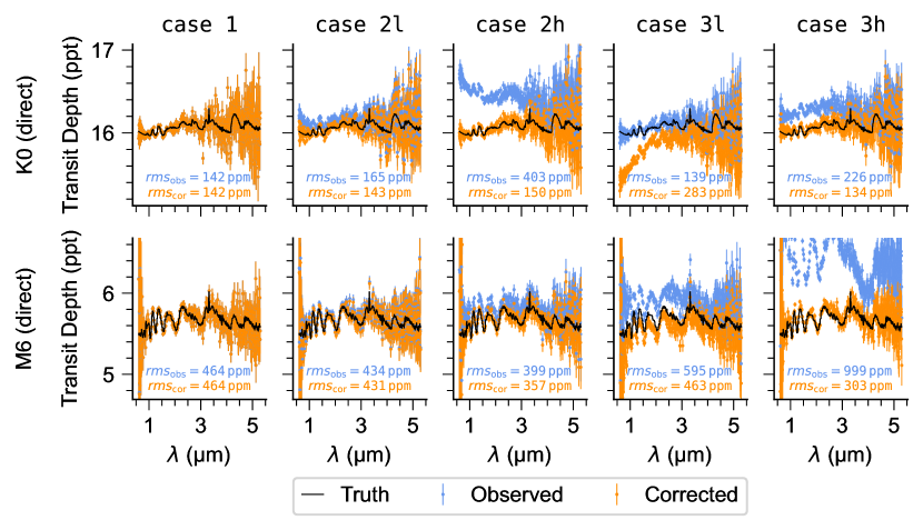
Figure 5 shows the observed and corrected transmission spectra from the direct retrievals using the model complexities identified in Section 4.1. To assess the change in bias, we calculated the root-mean-square (rms) residual between the data and the model truth for both $D_{\mathrm{obs,\lambda}}$ and $D_{\mathrm{cor,\lambda}}$. We find that the corrections reduce the bias in the transmission spectra in 7 of 8 spectra (no corrections are possible for another two spectra from case 1, for which stellar contamination is not an issue and $\epsilon_{\lambda}=1$ by definition). In these seven cases, the correction reduced the root-mean-squared (rms) residual between the data and the true planetary transmission spectrum by 177 ppm on average, with the smallest reduction being 3 ppm (M6 case 2l) and the largest being 696 ppm (M6 case 3h).

The case for which the correction procedure actually increased the bias in the transmission spectrum was the K0 3l case. As a reminder, the input parameters for the K0 simulations were $T_{\mathrm{phot}}=5270$ K, $T_{\mathrm{spot}}=3830$ K, and $T_{\mathrm{fac}}=5380$ K with $f_{\mathrm{spot}}$ and $f_{\mathrm{fac}}$ of 1% and 10% in case 3l. While the model comparison identified the correct level of complexity here, the algorithm identified another combination of three component spectra that satisfactorily describes the integrated spectrum, leading to an improper correction. This provides an interesting counterpoint to the example of the M6 case 3l spectrum, for which the 4-comp model was preferred (Section 4.1). In this case, the incorrectly identified 4-comp still lead to an rms bias reduction of 132 ppm, whereas the 3-comp model, which had the appropriate complexity but the wrong inferred parameters, would have led to an rms bias reduction of only 96 ppm, if selected. Relying on “perfect” spectral models but producing incorrect inferences, these results both underscore the limitations of this approach in general in this highly complicated parameter space, a point we return to in the discussion.

4.3 Impact on the Uncertainty Budget

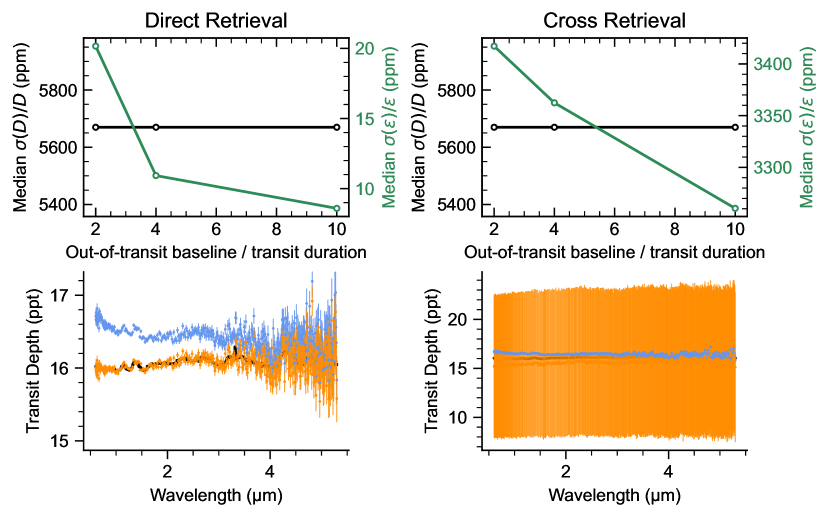
The final result that we consider here is the impact on the uncertainty budget. We are interested in the impact of applying the derived corrections from the selected models for the stellar photosphere and propagating their uncertainties on the final uncertainties of the transmission spectra. Figure 6 illustrates the most salient point in this context, which is that the ultimate uncertainty contribution of model-based corrections for stellar contamination depends strongly on how well the models are able to describe the true spectra behind the data (i.e., the “model fidelity”). Focusing on the M6 case 2h dataset, this figure shows that in the case of the direct retrieval the relative uncertainty on $\epsilon$ is vanishingly small compared to that on $D$, owing to the high degree of fidelity between the synthetic stellar spectrum and the PHOENIX-based retrieval, leading to a correction that imparts no notable additional uncertainty on the final transmission spectrum. In this case and all other direct-retrieval cases, the median per-point uncertainty of the transmission spectrum increased by no more than 1 ppm. On the other hand, in the cross-retrieval case the relative uncertainty on $\epsilon$ is two orders of magnitude larger, stemming from the need to inflate uncertainties to produce adequate fits, and thus the stellar-contamination correction dominates the final uncertainty of the transmission spectrum.

We also explored how these results depend on the duration of the out-of-transit baseline, repeating our entire retrieval analysis with simulated datasets that had two and five times longer out-of-transit baselines (four and ten times the transit duration, respectively). We find that the uncertainties on $\epsilon$ decreases with increasing baseline, as expected, but that the final uncertainties on the corrected transmission spectra remain high in the case of the cross retrievals, owing to the need to compensate for model differences with inflated uncertainties. Nonetheless, we note that in “real life” applications, the lack of model fidelity and other effects (such as stellar variability) may make the need for longer baselines more pressing.

Figure 6: Median uncertainties of the transmission spectrum ($D$) and the stellar contamination signal ($\epsilon$) for the K0 case 2h dataset. The left (right) column shows result for the direct (cross) retrieval of the dataset with the 2-comp model, which was the preferred model complexity in both cases. In the top row, the black points show the median fractional uncertainty on the transit depth as a function of the out-of-transit baseline, and the green points show the same for the stellar contamination signal. The fraction uncertainty of the stellar contamination signal is consistently smaller and decreases with increasing out-of-transit baseline, as expected. The bottom row shows the true (black), observed (blue), and corrected (orange) transmission spectra resulting from these retrievals. The results of the direct retrieval show that when the model fidelity is sufficient, the contribution of the stellar-contamination correction to the noise budget of the planetary spectrum is negligible. By contrast, the results of the cross retrieval show that while the uncertainty on the stellar contamination signal appears to be on the same order of magnitude as the transit depth uncertainties, the uncertainty inflation necessary to provide an adequate fit of the stellar spectrum actually leads the poorly constrained stellar contamination signal to dominate the final uncertainties of the transmission spectrum.

Figure 7: Flux changes due to temperature variations for the range of stellar models we consider. The left column shows PHOENIX models relevant to our K0 case, and the right shows PHOENIX models relevant to our M6 case. The top panels show the spectra in absolute flux units, while the bottom panels show each set normalized to the middle-temperature model in each set. The wavelengths and resolution of the spectra are relevant to NIRSpec/PRISM. Larger flux differences are evident for the set of models relevant to the M6 case, which lead to more successful inferences from the retrievals.

5 Conclusions & Future Work

We investigated the use of out-of-transit stellar spectra to enhance JWST’s scientific return while reducing biases in exoplanet transmission spectra, with a focus on the impact of stellar model fidelity. Our analysis produced two primary findings.

1. The fidelity of stellar models is crucially important for identifying the right complexity of a photosphere and deriving appropriate corrections for transmission spectra. The differences between existing model grids dominate by orders of magnitude the total noise budget. This translates into needing to inflate photon-noise errorbars by orders of magnitude (Figure 6), which prevents efforts from harnessing the full potential of JWST for transits of stars with heterogeneous photospheres. We note that even when accounting for this inflation, significant biases on the derived properties of the stellar photosphere are possible, leading to improper corrections. This finding is similar to earlier findings of de Wit et al. (2012) and N22, which have shown that an apparently good fit can hide a compensation for a model’s lack of fidelity via biases in the model parameters.

2. If the model fidelity is on par with the precision of the spectra, it is possible to reliably infer the correct model parameters (including the true number of components). This means that with sufficient model fidelity, one can expect to correct for stellar contamination to the maximum extent possible, given the information content of the data, and there is no model-driven bottleneck. In this context, we show that the uncertainty associated with the correction of the stellar contamination is marginal compared to the photon noise on the transmission spectrum, thereby allowing photon-limited science (i.e., harnessing the full potential of JWST).

These findings should motivate both further theoretical developments in modeling the spectra of stars and their heterogeneities, as well as new observation strategies to derive empirical constraints on stellar photospheric heterogeneity from highly precise JWST spectra. In fact, we suggest that observational strategies could be developed to acquire these empirical constraints with the observatories with which the planetary atmospheres will be explored to ensure a “fidelity” on par with the data driving the atmospheric characterization. We provide in the following a few additional considerations for future works.

5.1 Spectral Model Grids and Interpolation Schemes

Our posterior inferences on component temperatures are roughly 2 K, while the spacing of the temperature grids is 100 K for all three model grids used. This means that the sampling of the model grid is insufficient for the high-SNR data at hand. In addition, we use a linear interpolation scheme for simplicity, which could also contribute to reducing the fidelity of the models over the coarse grid available (see, e.g., Czekala et al., 2015). In order to support the reliable correction of stellar contamination in JWST exoplanet transmission spectra, we suggest it would be useful to generate model grids with spacings in each of their dimensions that are two orders of magnitude smaller than those currently available. We also recommend that future work explore the impact in this context of linear interpolation versus more complex approaches, such as bicubic interpolation or spectral emulation via principal component analysis (e.g., Czekala et al., 2015).

5.2 Heterogeneities Are Not Your Average Photosphere

Out-of-transit spectra are currently fitted using a combination of stellar spectra weighted by different filling factors. This approach thus assumes that spot and faculae spectra can be approximated by stellar spectra derived from 1D radiative–convective models. Although this assumption may be passable for spots (Rackham et al., 2022), it has been shown to be a poor assumption for facula spectra, which contain magnetically induced features that are not captured well by the simplified 1D models (Witzke et al., 2022). The increased differentiation of a component’s features, while more problematic because the components are more challenging to approximate with current models, will also make their contribution easier to disentangle in observations. While a new generation of calculations for the spectra of heterogeneities are underway (e.g., with MPS-ATLAS; Witzke et al., 2021), the prospect of supporting the benchmarking of said models with empirical constraints within reach with JWST is tantalizing.

5.3 When Worse Can Also Mean Better

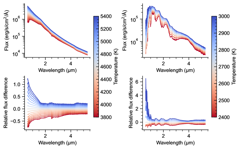
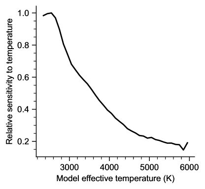
As with facula spectra, for which the challenge of fitting them is also a unexpected benefit, the challenge of constraining photospheric heterogeneity in cooler stars may be lessened by that same heterogeneity. In Section 4.2 we found that the correction derived from the direct retrieval of the K0 case 3l spectrum actually increased the bias in the transmission spectrum, owing to incorrect inferences derived from the out-of-transit stellar spectrum. Ultimately, these incorrect inferences deriving from high-SNR spectra simulated and fitted with the same spectral grid highlight the challenge of deriving constraints in this temperature regime. Figure 7 shows the sensitivity of stellar spectra to temperature variations over ranges covering the components of our K0 and M6 cases. It highlights that the sensitivity of the spectra relevant to a K0 and its photospheric components is smaller than for the M6 case (Figure 8), which relates to the expectation of a lower level of stellar contamination. Yet, the strength of temperature-sensitive features in the spectra actually support the detection and characterization of these heterogeneities, and thus the correction of stellar contamination. Thus, we note that the lack of significant differentiation in the K0 models can also lead to biased inferences when a particular noise realization permits another nearby, nearly blackbody model to fit the data, though working at higher resolving power with other JWST observational modes (e.g., NIRSpec/G395H, NIRISS SOSS) will likely help here.

Figure 8: The sensitivity of PHOENIX stellar models, sampled at the wavelength range and resolution NIRSpec/PRISM, to changes in stellar temperature. The relative change in stellar flux is shown as a function of the model effective temperature, normalized to the value for a model of 2500 K. The sensitivity to temperature decreases with increasing temperature, with models around 6000 K displaying roughly 20% of the sensitivity of the 2500 K model.

5.4 Empirical Heterogeneity Constraints

We have worked under the assumption that different stellar model grids are equally good. Another possibility is that advances, including among other things updated opacities for a wide range of sources (e.g., Tennyson et al., 2016, 2020; Gordon et al., 2017, 2022), have allowed more recent grids to more closely resemble reality. In this case, the differences between model grids then reflect the growth in our understanding rather than a remaining understanding gap to cross. To assess this possibility, we recommend that these techniques be applied to real JWST data, starting with an inactive star and advancing to more active stars to understand the limits of model-based inferences with real data—keeping in mind that a “good fit” does not automatically imply “model fidelity.” We also recommend the exploration of empirical approaches for deriving the unique spectral components of a photosphere and their filling factors, enabling corrections that are independent of spectral models.

References

- Afram & Berdyugina (2015) Afram, N., & Berdyugina, S. V. 2015, A&A, 576, A34, doi: 10.1051/0004-6361/201425314
- Ahrer et al. (2023) Ahrer, E.-M., Stevenson, K. B., Mansfield, M., et al. 2023, Nature, 614, 653, doi: 10.1038/s41586-022-05590-4
- Alderson et al. (2023) Alderson, L., Wakeford, H. R., Alam, M. K., et al. 2023, Nature, 614, 664, doi: 10.1038/s41586-022-05591-3
- Batalha et al. (2017) Batalha, N. E., Mandell, A., Pontoppidan, K., et al. 2017, PASP, 129, 064501, doi: 10.1088/1538-3873/aa65b0
- Bean et al. (2018) Bean, J. L., Stevenson, K. B., Batalha, N. M., et al. 2018, PASP, 130, 114402, doi: 10.1088/1538-3873/aadbf3
- Benneke & Seager (2013) Benneke, B., & Seager, S. 2013, ApJ, 778, 153, doi: 10.1088/0004-637X/778/2/153
- Brown (2001) Brown, T. M. 2001, ApJ, 553, 1006, doi: 10.1086/320950
- Buchner (2014) Buchner, J. 2014, arXiv e-prints, arXiv:1407.5459, doi: 10.48550/arXiv.1407.5459
- Buchner (2017) —. 2017, arXiv e-prints, arXiv:1707.04476, doi: 10.48550/arXiv.1707.04476
- Buchner (2021) —. 2021, The Journal of Open Source Software, 6, 3001, doi: 10.21105/joss.03001
- Czekala et al. (2015) Czekala, I., Andrews, S. M., Mandel, K. S., Hogg, D. W., & Green, G. M. 2015, ApJ, 812, 128, doi: 10.1088/0004-637X/812/2/128
- de Wit et al. (2012) de Wit, J., Gillon, M., Demory, B. O., & Seager, S. 2012, A&A, 548, A128, doi: 10.1051/0004-6361/201219060
- Feinstein et al. (2023) Feinstein, A. D., Radica, M., Welbanks, L., et al. 2023, Nature, 614, 670, doi: 10.1038/s41586-022-05674-1
- Foreman-Mackey et al. (2013) Foreman-Mackey, D., Hogg, D. W., Lang, D., & Goodman, J. 2013, PASP, 125, 306, doi: 10.1086/670067
- Foreman-Mackey et al. (2019) Foreman-Mackey, D., Farr, W., Sinha, M., et al. 2019, The Journal of Open Source Software, 4, 1864, doi: 10.21105/joss.01864
- Fu et al. (2022) Fu, G., Espinoza, N., Sing, D. K., et al. 2022, ApJ, 940, L35, doi: 10.3847/2041-8213/ac9977
- Garcia et al. (2022) Garcia, L. J., Moran, S. E., Rackham, B. V., et al. 2022, A&A, 665, A19, doi: 10.1051/0004-6361/202142603
- Gillon et al. (2016) Gillon, M., Jehin, E., Lederer, S. M., et al. 2016, Nature, 533, 221, doi: 10.1038/nature17448
- Gillon et al. (2017) Gillon, M., Triaud, A. H. M. J., Demory, B.-O., et al. 2017, Nature, 542, 456, doi: 10.1038/nature21360
- Gordon et al. (2017) Gordon, I. E., Rothman, L. S., Hill, C., et al. 2017, J. Quant. Spec. Radiat. Transf., 203, 3, doi: 10.1016/j.jqsrt.2017.06.038
- Gordon et al. (2022) Gordon, I. E., Rothman, L. S., Hargreaves, R. J., et al. 2022, J. Quant. Spec. Radiat. Transf., 277, 107949, doi: 10.1016/j.jqsrt.2021.107949
- Husser et al. (2013) Husser, T. O., Wende-von Berg, S., Dreizler, S., et al. 2013, A&A, 553, A6, doi: 10.1051/0004-6361/201219058
- Iyer & Line (2020) Iyer, A. R., & Line, M. R. 2020, ApJ, 889, 78, doi: 10.3847/1538-4357/ab612e
- Iyer et al. (2023) Iyer, A. R., Line, M. R., Muirhead, P. S., Fortney, J. J., & Gharib-Nezhad, E. 2023, ApJ, 944, 41, doi: 10.3847/1538-4357/acabc2
- JWST Transiting Exoplanet Community Early Release Science Team et al. (2023) JWST Transiting Exoplanet Community Early Release Science Team, Ahrer, E.-M., Alderson, L., et al. 2023, Nature, 614, 649, doi: 10.1038/s41586-022-05269-w
- Kostogryz et al. (2023) Kostogryz, N., Shapiro, A. I., Witzke, V., et al. 2023, Research Notes of the American Astronomical Society, 7, 39, doi: 10.3847/2515-5172/acc180
- McCullough et al. (2014) McCullough, P. R., Crouzet, N., Deming, D., & Madhusudhan, N. 2014, ApJ, 791, 55, doi: 10.1088/0004-637X/791/1/55
- Niraula et al. (2022) Niraula, P., de Wit, J., Gordon, I. E., et al. 2022, Nature Astronomy, doi: 10.1038/s41550-022-01773-1
- Pecaut & Mamajek (2013) Pecaut, M. J., & Mamajek, E. E. 2013, ApJS, 208, 9, doi: 10.1088/0067-0049/208/1/9
- Rackham et al. (2018) Rackham, B. V., Apai, D., & Giampapa, M. S. 2018, ApJ, 853, 122, doi: 10.3847/1538-4357/aaa08c
- Rackham et al. (2019) —. 2019, AJ, 157, 96, doi: 10.3847/1538-3881/aaf892
- Rackham et al. (2022) Rackham, B. V., Espinoza, N., Berdyugina, S. V., et al. 2022, arXiv e-prints, arXiv:2201.09905, doi: 10.48550/arXiv.2201.09905
- Rustamkulov et al. (2022) Rustamkulov, Z., Sing, D. K., Liu, R., & Wang, A. 2022, ApJ, 928, L7, doi: 10.3847/2041-8213/ac5b6f
- Rustamkulov et al. (2023) Rustamkulov, Z., Sing, D. K., Mukherjee, S., et al. 2023, Nature, 614, 659, doi: 10.1038/s41586-022-05677-y
- Seager & Sasselov (2000) Seager, S., & Sasselov, D. D. 2000, ApJ, 537, 916, doi: 10.1086/309088
- Sing et al. (2011) Sing, D. K., Pont, F., Aigrain, S., et al. 2011, MNRAS, 416, 1443, doi: 10.1111/j.1365-2966.2011.19142.x
- Tennyson et al. (2016) Tennyson, J., Yurchenko, S. N., Al-Refaie, A. F., et al. 2016, Journal of Molecular Spectroscopy, 327, 73, doi: 10.1016/j.jms.2016.05.002
- Tennyson et al. (2020) —. 2020, J. Quant. Spec. Radiat. Transf., 255, 107228, doi: 10.1016/j.jqsrt.2020.107228
- Trotta (2008) Trotta, R. 2008, Contemporary Physics, 49, 71, doi: 10.1080/00107510802066753
- Wakeford et al. (2019) Wakeford, H. R., Lewis, N. K., Fowler, J., et al. 2019, AJ, 157, 11, doi: 10.3847/1538-3881/aaf04d
- Witzke et al. (2022) Witzke, V., Shapiro, A. I., Kostogryz, N. M., et al. 2022, ApJ, 941, L35, doi: 10.3847/2041-8213/aca671
- Witzke et al. (2021) Witzke, V., Shapiro, A. I., Cernetic, M., et al. 2021, A&A, 653, A65, doi: 10.1051/0004-6361/202140275
- Zhang et al. (2018) Zhang, Z., Zhou, Y., Rackham, B. V., & Apai, D. 2018, AJ, 156, 178, doi: 10.3847/1538-3881/aade4f