NeUDF: Learning Unsigned Distance Fields from Multi-view Images for Reconstructing Non-watertight Models
Abstract
Volume rendering-based 3D reconstruction from multi-view images has gained popularity in recent years, largely due to the success of neural radiance fields (NeRF). A number of methods have been developed that build upon NeRF and use neural volume rendering to learn signed distance fields (SDFs) for reconstructing 3D models. However, SDF-based methods cannot represent non-watertight models and, therefore, cannot capture open boundaries. This paper proposes a new algorithm for learning an accurate unsigned distance field (UDF) from multi-view images, which is specifically designed for reconstructing non-watertight, textureless models. The proposed method, called NeUDF, addresses the limitations of existing UDF-based methods by introducing a simple and approximately unbiased and occlusion-aware density function. In addition, a smooth and differentiable UDF representation is presented to make the learning process easier and more efficient. Experiments on both texture-rich and textureless models demonstrate the robustness and effectiveness of the proposed approach, making it a promising solution for reconstructing challenging 3D models from multi-view images.
1 Introduction
 |
 |
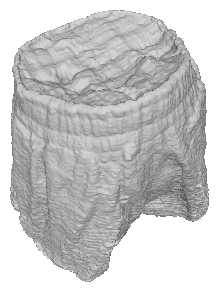 |
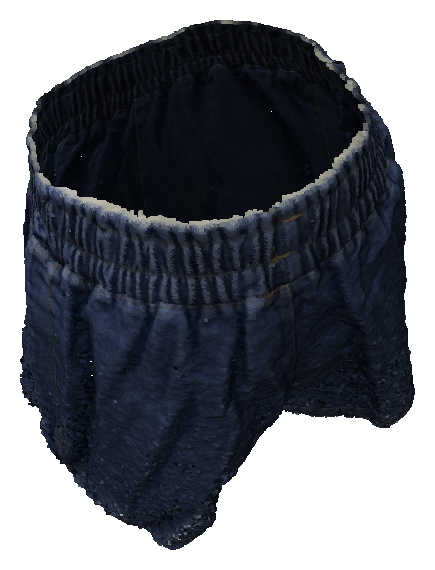
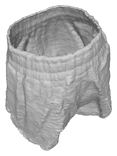
| Reference Image | Ours | NeuS [33] |
In recent years, volume rendering-based 3D model and scene reconstruction from multi-view images has gained popularity, largely due to the success of neural radiance fields (NeRF) [27]. A number of methods have been developed that build upon NeRF and use neural volume rendering to learn signed distance fields (SDFs) for reconstructing 3D models [37, 33, 35, 7]. While these SDF-based methods are effective in reconstructing watertight models, they cannot represent non-watertight models, as SDFs distinguish between the interior and exterior of a model, and therefore cannot capture open boundaries.
Recent research has attempted to address the limitation of signed distance fields in reconstructing non-watertight models by using unsigned distance fields (UDFs). For instance, NeuralUDF [22] extends NeuS [33] to learn UDFs for reconstructing open models. However, UDF-based methods have their own limitations. For example, as shown in Figure 1, NeuralUDF struggles to reconstruct textureless models or models with few distinguishable features, as it relies on texture information to improve the accuracy of reconstruction. Also, UDF is not differentiable at the zero level-set, making it difficult to learn. Reconstructing open, textureless models from multi-view images using volume rendering remains a challenging problem.
We propose a new algorithm for learning an accurate UDF from multi-view images, which we call NeUDF. Our method is specifically designed for reconstructing non-watertight, textureless models, which are particularly challenging to reconstruct using existing UDF-based methods. The key to learning an accurate UDF is to design an unbiased and occlusion-aware density function of the UDF. Since the inside and outside of the model are not distinguished, the S-shape density function used in SDF-based methods [33] is not appropriate for UDFs. Long et al. [22] proposed a piecewise density function adapted from NeuS [33], but this function is rather complicated and difficult to learn, limiting its applicability to texture-rich models.
To overcome these limitations, we propose a new UDF density function for learning UDFs, which can tolerate a small amount of bias to ease learning. Our density function is dense enough to be almost opaque, making it occlusion-aware and effective for reconstructing non-watertight models. Additionally, we present a smoothed UDF representation that makes the UDF differentiable at the zero level set, which is crucial for the learning process. We evaluate our proposed approach on both texture-rich and textureless models from the DeepFashion3D [41] and DTU [17] datasets. Our experiments demonstrate that our method is robust and can effectively learn UDFs for both types of inputs.
Our work makes the following contributions:
-
1.
We propose a method for reconstructing non-watertight models based on NeRF that is capable of reconstructing both texture-rich and challenging textureless models.
-
2.
We introduce a theoretically sound density function for UDFs and in practice adopt a variant that allows a small bias and is approximately occlusion-aware.
-
3.
We present a smooth and differentiable UDF representation that makes the learning process easier and more efficient.
-
4.
We present a simple yet effective method for extracting the target surface from the learned UDFs, which can reduce the bias.
2 Related Work
2.1 3D Reconstruction from Multi-View Images
Surface reconstruction from multi-view images has been a subject of study for several decades, and can generally be classified into two categories: voxel-based and point-based methods. Voxel-based methods [2, 3, 18, 19, 32] divide the 3D space into voxels and determine which ones belong to the object. These methods can be computationally expensive and may not be suitable for reconstructing complex surfaces. Point-based methods [12, 30, 36] use structure-from-motion [15] to calibrate the images and generate a dense point cloud using multi-view stereo [11]. Finally, surface reconstruction methods (e.g., [1, 20, 16]) are used to generate a mesh. Since multi-view stereo requires dense correspondences to generate a dense point cloud, which are often difficult to compute, its results often contain various types of artifacts, such as noise, holes and incomplete structures.
Neural network-based 3D surface reconstruction has received attention in recent years with the emergence of neural rendering [27]. Several methods have been proposed for volume rendering and surface reconstruction using neural networks. VolSDF [37] uses the cumulative distribution function of Laplacian distribution to evaluate the density function from SDF for volume rendering and surface reconstruction. NeuS [33] adopts an unbiased density function for SDFs for more accurate reconstruction. SparseNeuS [23] extends NeuS to use fewer images for reconstruction. HF-NeuS [35] improves NeuS by proposing a simplified and unbiased density function and using hierarchical MLPs for detail reconstruction. Geo-NeuS [9] incorporates structure-from-motion to add more constraints. NeuralWarp [7] improves the accuracy by optimizing consistency between warped views of different images. All of these methods learn SDFs, which can only reconstruct watertighjt models.
More recently, Long et al. proposed NeuralUDF [22] for learning UDF for reconstructing open models. It adapts the density function of NeuS to UDFs by introducing an indicator function. However, this method can only learn texture-rich models due to the complex density function used in training. In contrast, our proposed UDF learning method is capable of reconstructing both texture-rich and textureless models without the need for masks.
2.2 3D Reconstruction from Point Clouds
There has been recent interest in surface representation using signed distance fields (SDFs) and occupation fields. Several methods have been proposed for learning SDFs [28, 4, 31, 24, 34], while occupation fields have been used in methods such as [26, 5]. However, both SDFs and occupation fields can only represent watertight models.
3 Method
Our goal is to extract a set of surface points from a set of input images along with their corresponding known camera poses and intrinsic parameters. To achieve this, we first learn an implicit unsigned distance field, whose zero level set represents the 3D surface. Unlike signed distance fields, UDFs have positive distance values, making them suitable for representing non-watertight models. However, learning a UDF from multi-view images is a challenging task that requires a proper density function balancing occlusion-awareness, ease of learning, and unbiasedness. Another technical issue is that UDFs are not differentiable at the zero level-set, making it difficult to train. Our proposed method is designed to address the above challenges of learning UDFs from multi-view images.
In this section, we first review the key concepts of volume rendering and neural radiance fields. Next, we propose an unbiased density function and use its variant to balance the density properties for UDF learning. We then introduce a differentiable form of UDF that can be used for stable learning. Finally, we detail our loss function design.
3.1 Review of Volume Rendering
Volume rendering is a crucial component of neural radiance fields [27]. During volume rendering, a ray is cast from the camera position to each pixel of the virtual canvas. The direction of the ray is denoted by , and any point along the ray can be expressed as , where is the arc-length parameter. In the following, we refer to the point using the parameter if there is no confusion.
The color of the corresponding pixel is determined by the color of the ray, which is the weighted integral of all colors along the ray ,
The integral is often computed numerically using quadrature, which is a sum of color values at a set of sampled points on the ray, i.e.,
The weight of each color value is the product between the volume density and transparency [25] , which measures the accumulated transmittance and occlusion of the ray up to that point. The transparency , which is defined as is the probability that the ray travels from to without hitting any other particle. is a monotonic decreasing function with a starting value of .
In NeRF [27], the volume density is directly computed by a multi-layer perceptron (MLP), which takes the 3D coordinates of a point as input and outputs the corresponding density value. This allows for a flexible representation of the volume density field and enables the synthesis of novel views from arbitrary viewpoints. However, since the volume density field does not provide explicit information about the surface geometry, extracting a high-quality surface from it is difficult. Moreover, the density field may not correspond to a valid surface at all due to the ill-posed nature of the reconstruction problem [38].
To overcome this limitation, NeuS [33] utilizes signed distance functions to represent 3D geometry. Specifically, it uses a scalar function that maps each point in 3D space to the signed distance from that point to the surface, where the zero level set of the function represents the target surface. It then maps the signed distance function to an S-density function using a logistic density distribution , which assigns a normalized density value to each point in space based on its signed distance from the surface. The normalized S-density function is then used to define the weight function for volume rendering.
Wang et al. [33] proved that the weight function in NeuS is both unbiased and occlusion-aware. Being unbiased means that the weight function attains a locally maximal value at a surface intersection point, while an occlusion-aware weight function implies that when two points have the same SDF value, the point closer to the viewpoint has a larger contribution to the output color than the other point. This accounts for the occlusion effect, where points behind the surface are not visible and should not contribute to the output color.
3.2 Density Function
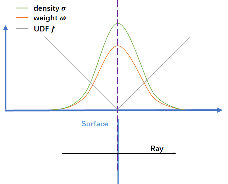
A core part of NeUDF is an unbiased and occlusion-aware weight function. Inspired by HF-NeuS [35], we propose a bell-shaped weight function that maps unsigned distance to density. Our weight function is unbiased in that the weights are maximum on the surface.

(a) (b)
Theorem 1.
A ray hits a planar object . Let be the angle between the UDF gradient and the ray direction . Define the bell-shaped density as
| (1) |
where is a learnable parameter. Then the weight function is unbiased.
Proof.
Let be the intersection point.
We first consider the transparency with , i.e., for any point along the ray up to . Since the point is in front of , we have and . The transparency , , is given by
Next we compute the weight function , which is proportional to
It is straightforward to verify that the sign of is the same as . Using the chain rule, we can show that the derivative is positive for , implying that the weight increases as the ray approaches from the front.
After the ray passes through , becomes positive and both and are monotonically decreasing for . Therefore, the product decreases as the ray leaves .
Since the weight is continuous, attains its maximum on the plane , implying that it is unbiased. ∎
The density function in Equation (1) is theoretically sound, satisfying the requirements of unbiased sampling. However, in practice, it may be too “transparent” to use (due to its bell-shaped geometry), leading to poor sampling efficiency. Moreover, the dependence of the bell-shaped function on the UDF gradients, as indicated by the term, can introduce instability and sensitivity to noise and oscillations, thereby posing challenges in learning the function.
To address these issues, we replace the term with a constant , resulting in a modified density function
This modification increases both numerical stability and opacity of the original density function .
However, unlike the original density , the modified density introduces bias in the weight function, since the maximum value of weight occurs at a point in front of , which has a distance value
| (2) |
While the modified density function is not theoretically unbiased, setting as a small constant can greatly reduce the bias in practice. Additionally, we expect to be approximately occlusion-aware. To further understand the numerical properties of , we consider the extreme case where the incident light ray is perpendicular to the planar surface . In this case, the unsigned distance function is for points in front of . As is symmetric for the two sides of , the surface transparency is the square of the transparency of the front side. Our computation shows
and to reduce transparency, we should choose a relatively large .
In our implementation, we set the constant based on the typical value of the learned parameter , which ranges between and given that the models are learned in a unit sphere to become unitless. This enables us to estimate the upper bound of the bias. For points in front of the surface, the incident angle between the ray and the surface normal is obtuse, so we restrict to the range of . By setting , the offset width between 0.00161 and 0.00566 is obtained relative to the true zero level set, indicating that the maximum relative bias is below 0.5%. This error level is acceptable for most application scenarios. Moreover, the surface transparency in the extreme case mentioned above is less than . When a ray has a larger incident angle, its transparency becomes even smaller, resulting in an almost opaque density . As a result, the weight function is approximately occlusion-aware. Thus, setting the constant offers a good balance between occlusion-awareness and unbiasedness.
It is worth mentioning that our modified density function is much simpler than the density function used in NeuralUDF [22]. Although both densities introduce biases, we can control the bias of our density function within a very small range. In contrast, it is unclear what the range of bias is for the density function used in NeuralUDF. Thanks to the simplicity, our density function is easier to learn, thereby our method can work for a wider range of models. This includes textureless models, which pose challenges for NeuralUDF.
3.3 Training
Differentiable UDFs. NeuS uses an MLP network to learn the signed distance function , which is a differentiable function. In contrast, UDF is not differentiable at the zero level set, making the network difficult to learn the values and gradients of the UDF close to the zero level set.
Another crucial requirement is to ensure non-negative values for the computed distances, which seems a trivial task as one may simply apply absolute value or normalization such as ReLU to the MLP output. However, applying the absolute value to the distance is not viable due to its non-differentiability at zero. Similarly, normalizing the output value using ReLU is not feasible as it is also non-differentiable at zero, and its gradient vanishes for negative inputs. This can be particularly problematic for learning UDFs, since when the MLP returns a negative distance value, the ReLU gradient vanishes, hindering the update of the distance to a positive value in the subsequent iterations.
We add a softplus function after the output layer of the MLP. The softplus function [8] is a smooth and differentiable approximation of the ReLU function that is defined as
Softplus has the same shape as ReLU, but it is continuous and differentiable at every point, and its gradients do not vanish anywhere. Using the softplus function allows us to ensure that the output of the MLP is non-negative and differentiable, making it suitable for learning the UDF. We set in our experiments.
Loss functions. Following NeuralUDF [22], we adopt an iso-surface regularizer to penalize the UDF values of the non-surface points from being zero, therefore encouraging smooth and clean UDFs. The regularization loss is defined as [22]
where is a constant scalar that scales the learned UDF values, is the total number of sampled rays per training iteration, and is the number of sampled points on a single ray.
The value of , which is learnable in our method, significantly affects the quality of the reconstruction. When is small, it introduces a larger bias and leads to a more blurred output. We observe that typically converges to a relatively large value between 1000 and 2000, leading to visually pleasing results. However, in rare cases when stops increasing during training, we apply a penalty to force it to increase. The penalty is defined as follows
where is the number of rays during a training epoch. This term aggregates the reciprocals of all values used for the point on ray . Intuitively speaking, it encourages a larger during the early stage of training. In our implementation, we make this term optional since generally increases with a decreasing rate during training, and the penalty term is only necessary in rare cases when stops at a relatively low value.
As in other SDF- and UDF-based methods [33, 35, 22], we adopt color loss and Eikonal loss in our approach. Specifically, the color loss is the loss between the predicted color and the ground truth color of a single pixel as used in [33]. The Eikonal loss is used to regularize the learned distance field to have a unit gradient [13]. Putting it all together, we define the combined loss function as a weighted sum
where , , and are hyperparameters that control the weight of each loss term. In our experiments, we empirically set , , and , although is occasionally set to , and is optional.
Adaptive hierarchical sampling. We propose an adaptive hierarchical sampling (AHS) strategy for efficiently finding sample points along each ray for color computation. Existing approaches, such as NeuS [33] and NeuralUDF [22], adopt a fixed set of pre-defined sampling rates for all models, regardless of their geometry differences. They first uniformly sample 64 points on the ray and then iteratively conduct importance sampling on top of the coarse probability estimation. The sampling rate is doubled after each iteration, resulting in a maximum 512 samples on each ray.
We argue that an effective sampling strategy should be self-adaptive to geometry, which is connected to the learnable parameter . Essentially, a larger value of leads to a narrower bell-shaped density function, resulting in higher weights given to points closer to the surface and more concentrated samples on the surface. Our density function depends on the learnable parameter , which usually ranges between 1000 and 2000. We use the learned to guide more precise sample selection. Specifically, in the -th iteration of sampling, we set to , where is the maximum number of sampling iterations, which we set as in our implementation. During the early stage of training, when is still relatively small, we use the sampling rates as in NeuS and NeuralUDF. As the training progresses and the value of consistently increases, our adaptive sampling strategy is activated. Our ablation study confirms that adaptive hierarchical sampling increases the accuracy of our approach by up to 25%. See Section 4.3.
3.4 Surface Extraction
After learning the UDF , extracting the object surface is essential. Instead of extracting the zero level set of the function , we locate the sample points with the maximum weights to construct the surface. The reason for doing so is that extracting the zero level set from UDFs is notoriously unstable [14], often leading to artifacts such as holes, flipped triangles, and self-intersections in the output meshes.
The main technical challenge in locating the samples with maximum weights is that they depend on the view direction, due to the term in Equation (2). However, since our method penalizes small values of and yields a relatively large , the term has little effect to the distance value .
In our implementation, we obtain a subset of rays for each input image by uniformly sampling rays every pixels in both horizontal and vertical directions. For each ray , we sample points along it to find the location with the maximum weight. We classify the ray as a foreground ray if the sum of weights for the samples along inside the region of interest (a unit sphere centered at origin) is greater than 0.5. Otherwise, we consider as a background ray that misses the target object.
After collecting all foreground rays from all input images, we use the sample with the maximum weight for each ray as a surface point. Computational results show that our strategy is effective in producing satisfactory results (see Section 4.3).
4 Experiments
Implementation Details. The MLP for the UDF network consists of 8 hidden layers, each with 256 elements. We also use skip connections after every 4 hidden layers. The output of the UDF network is a single value representing the predicted UDF and a 256-dimensional feature vector used in the color network.
For the color network, we use another MLP with 4 hidden layers, each having 256 elements. We use the coarse-to-fine strategy proposed by Park et al. [29] for position encoding, setting the maximum number of frequency bands to 16 for the UDF network and 6 for the color network. For background rendering, we use NeRF++ [38] for background prediction. During training, we use the Adam optimizer [21] with a global learning rate of 5e-4. We sample 512 rays per batch and train our model for 300,000 iterations.
Data Sets. To evaluate our method, we use two datasets: DeepFashion3D [41] and DTU [17]. The DeepFashion3D dataset consists of clothing models, which are open models with boundaries. As only 3D points are available, we render 72 images of resolution with a white background from different viewpoints for each model. The DTU dataset consists of models captured in a studio, and all the models are watertight. We use this dataset to validate that our method also works well for watertight models. These datasets have been widely used in previous works such as [37, 33, 35].
Baselines. Several methods have been proposed for learning signed distance functions (SDFs) from multi-view images, which generate watertight models. To validate the effectiveness of our proposed method, we compare with state-of-the-art methods, namely VolSDF [37], NeuS [33], and HF-NeuS[35].
To our knowledge, NeuralUDF [22] 111Since the source code of NeuralUDF is unavailable at the moment of submission, we cannot make quantitative comparison with it in the paper. is the only method designed for open model reconstruction, but it is limited to texture-rich models. Our method, on the other hand, can reconstruct both textureless and texture-rich models thanks to the new and simpler density function we propose in this paper.
 |
 |
 |
| Reference Image | Ours | HF-NeuS [35] |
| Reference Image | GT | Ours | VolSDF [37] | NeuS [33] | HF-NeuS [35] | |
|---|---|---|---|---|---|---|
| #1 | 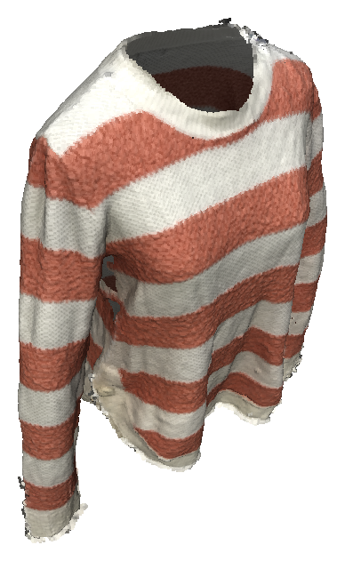 |
 |
 |
 |
 |
 |
| #5 | 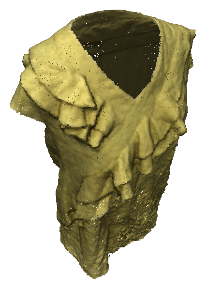 |
|
|
|
|
|
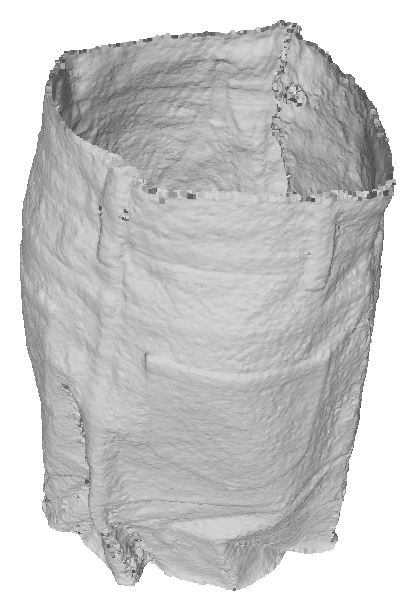
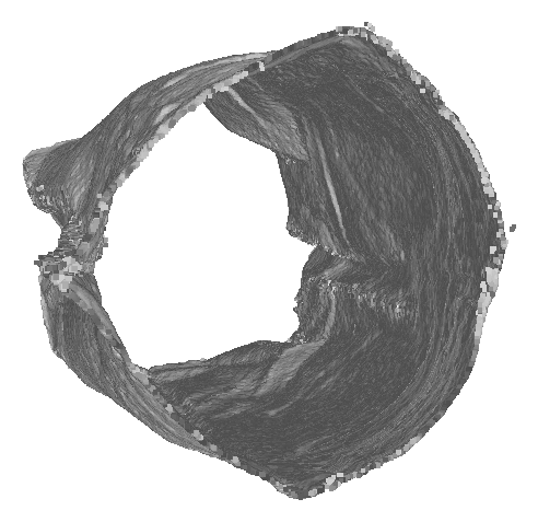
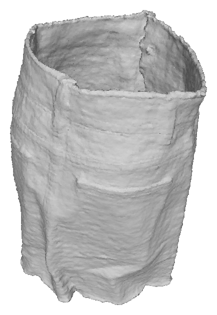
| #6 | 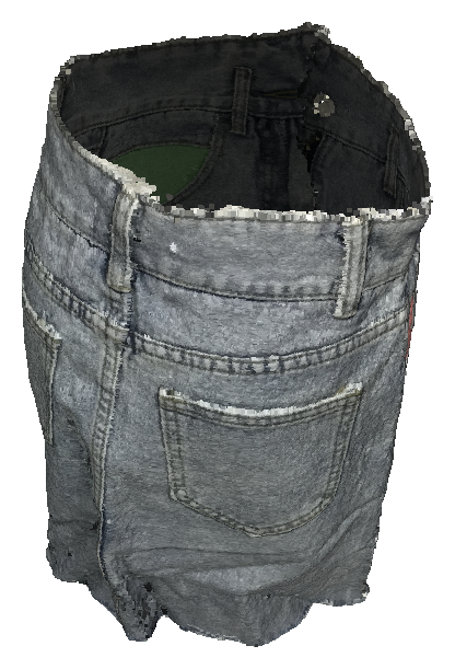 |
|
|
|
|
|
4.1 Comparisons on Open Models
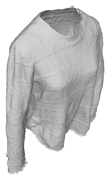
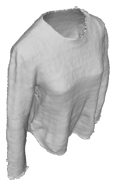
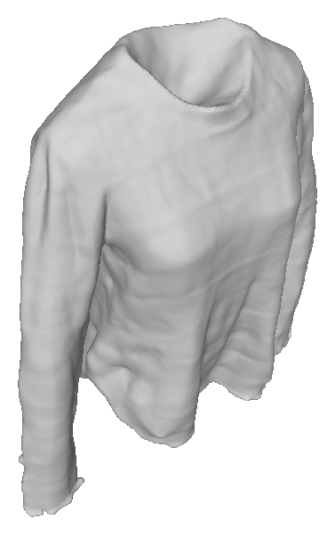
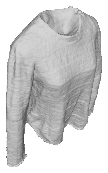
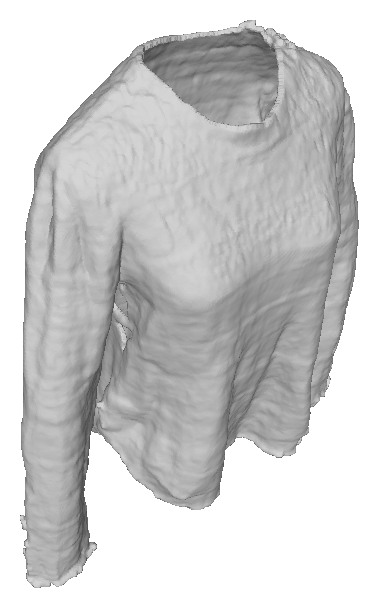
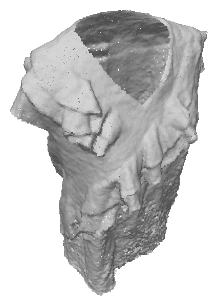
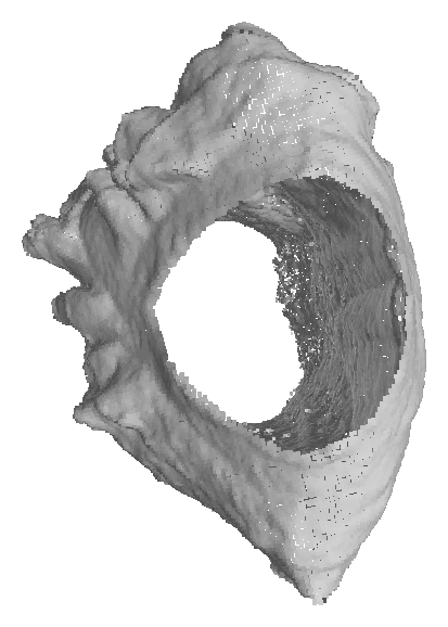
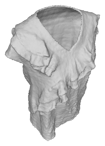
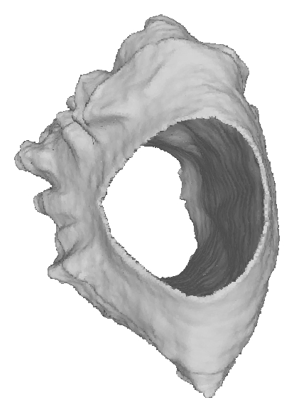
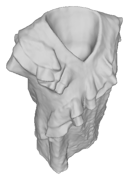
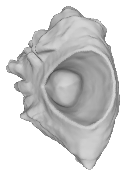
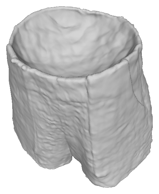
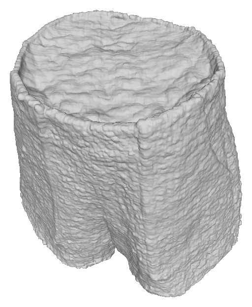
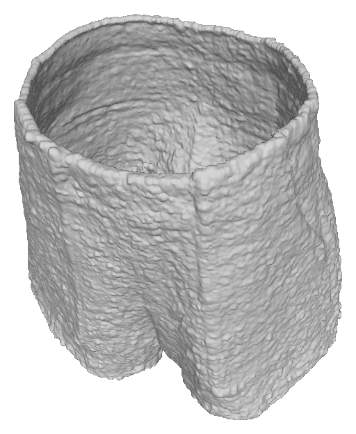
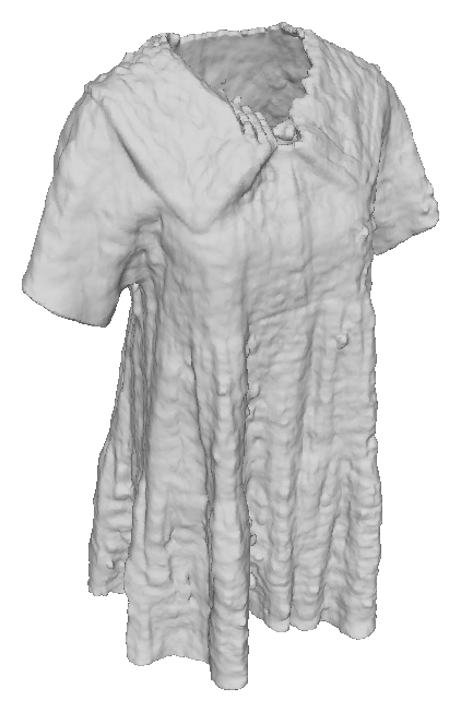
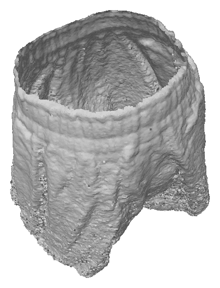
We evaluate our method and compare it with baselines using the clothes from DeepFashion3D, where the models have multiple open boundaries. VolSDF, NeuS, and HF-NeuS always close the boundaries since they learn SDFs. In contrast, our method learns UDFs, which can generate open models. Table 1 shows the point-to-point Chamfer distances of the results. Some of the Chamfer distances of the compared methods are large because the open holes are closed, resulting in significant errors.
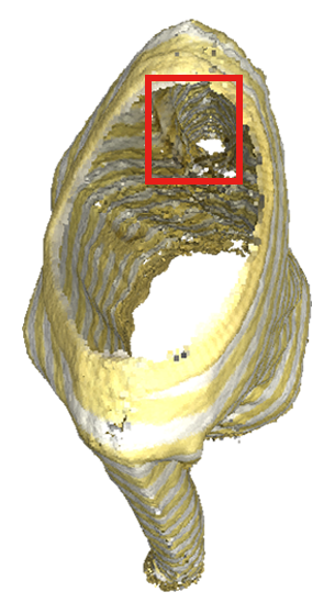
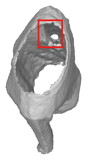
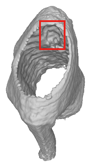
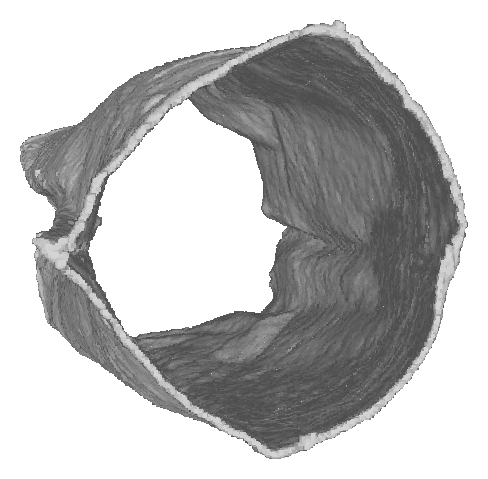
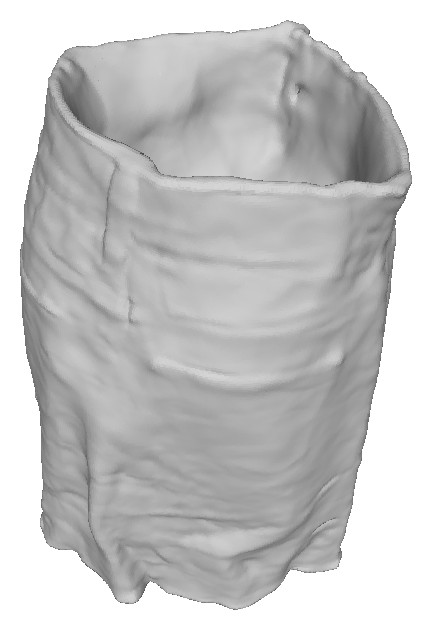
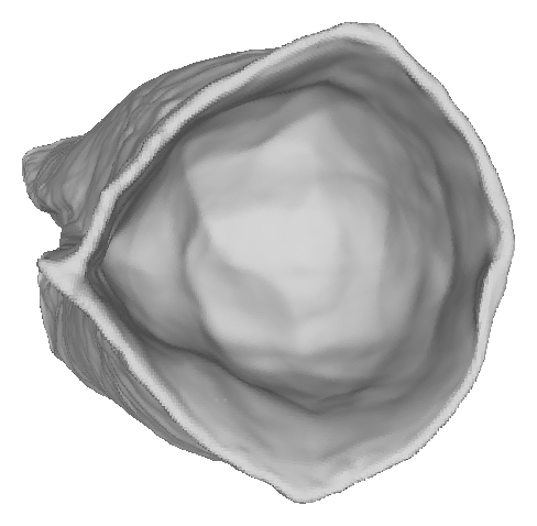
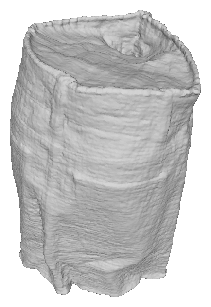
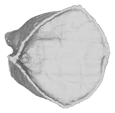
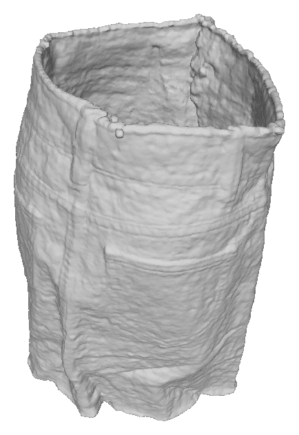
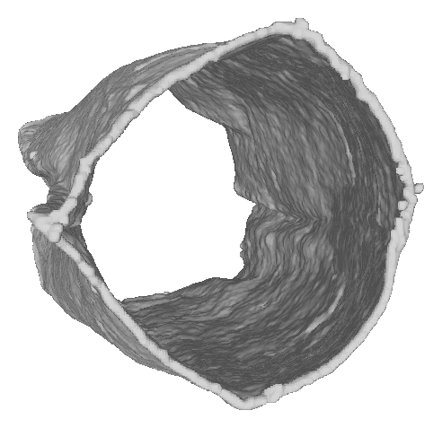
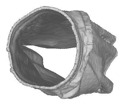
It is worth noting that HF-NeuS requires mask supervision to produce reasonable results on the DeepFashion3D dataset. With mask supervision, it is capable of producing double-covered surfaces that capture the geometric features well. However, these surfaces are still closed from a topological perspective, and their Chamfer distances are higher than those produced by our method. Additionally, the ability of HF-NeuS to generate valid results relies heavily on the mask; if the mask lacks boundary information, HF-NeuS may close the boundaries. For example, as shown in Figure 3, the sleeve structure is not labeled in the mask, resulting in a closed sleeve. In contrast, our method is able to properly reconstruct the open sleeve structure without relying on a mask.
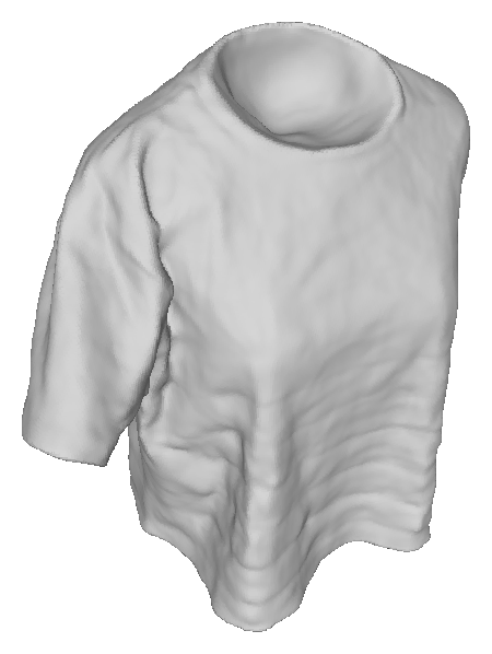
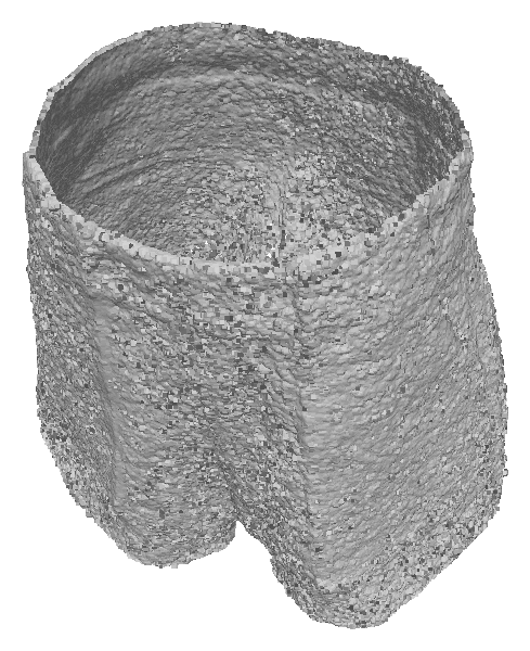
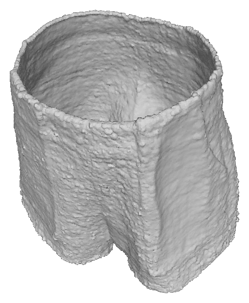
As demonstrated in Figure 4, we test various types of garments, some of which have rich textures, while others are nearly a single color. Learning UDFs for textureless models is more challenging since various regions of a model are ambiguous without clear color differences. However, our NeUDF generates satisfactory results even without masks. On the other hand, NeuralUDF [22] is unable to properly reconstruct textureless models, possibly due to their complex density function which is difficult to converge.
| Method | #1 | #2 | #3 | #4 | #5 | #6 | #7 | #8 | #9 | #10 | #11 | #12 | Mean |
|---|---|---|---|---|---|---|---|---|---|---|---|---|---|
| HF-NeuS [35] | 3.28 | 2.93 | 4.11 | 3.22 | 5.41 | 4.18 | 5.51 | 5.51 | 4.61 | 5.46 | 4.30 | 3.37 | 4.32 |
| VolSDF [37] | 6.22 | 5.75 | 9.45 | 8.33 | 8.99 | 16.37 | 17.01 | 5.95 | 12.88 | 9.08 | 17.39 | 11.54 | 10.75 |
| NeuS [33] | 6.75 | 4.60 | 4.35 | 7.95 | 13.52 | 10.74 | 14.54 | 6.23 | 16.69 | 17.07 | 13.21 | 5.13 | 10.07 |
| NeUDF w/ MeshUDF [14]) | 2.68 | 4.33 | 2.90 | 3.81 | 4.34 | 3.32 | 4.53 | 3.57 | 3.65 | 3.78 | 3.26 | 4.73 | 3.74 |
| NeUDF w/ max-weight | 2.09 | 1.77 | 1.75 | 2.00 | 2.34 | 2.16 | 3.54 | 2.60 | 2.81 | 3.63 | 2.64 | 2.61 | 2.50 |
4.2 Comparisons on Watertight Models
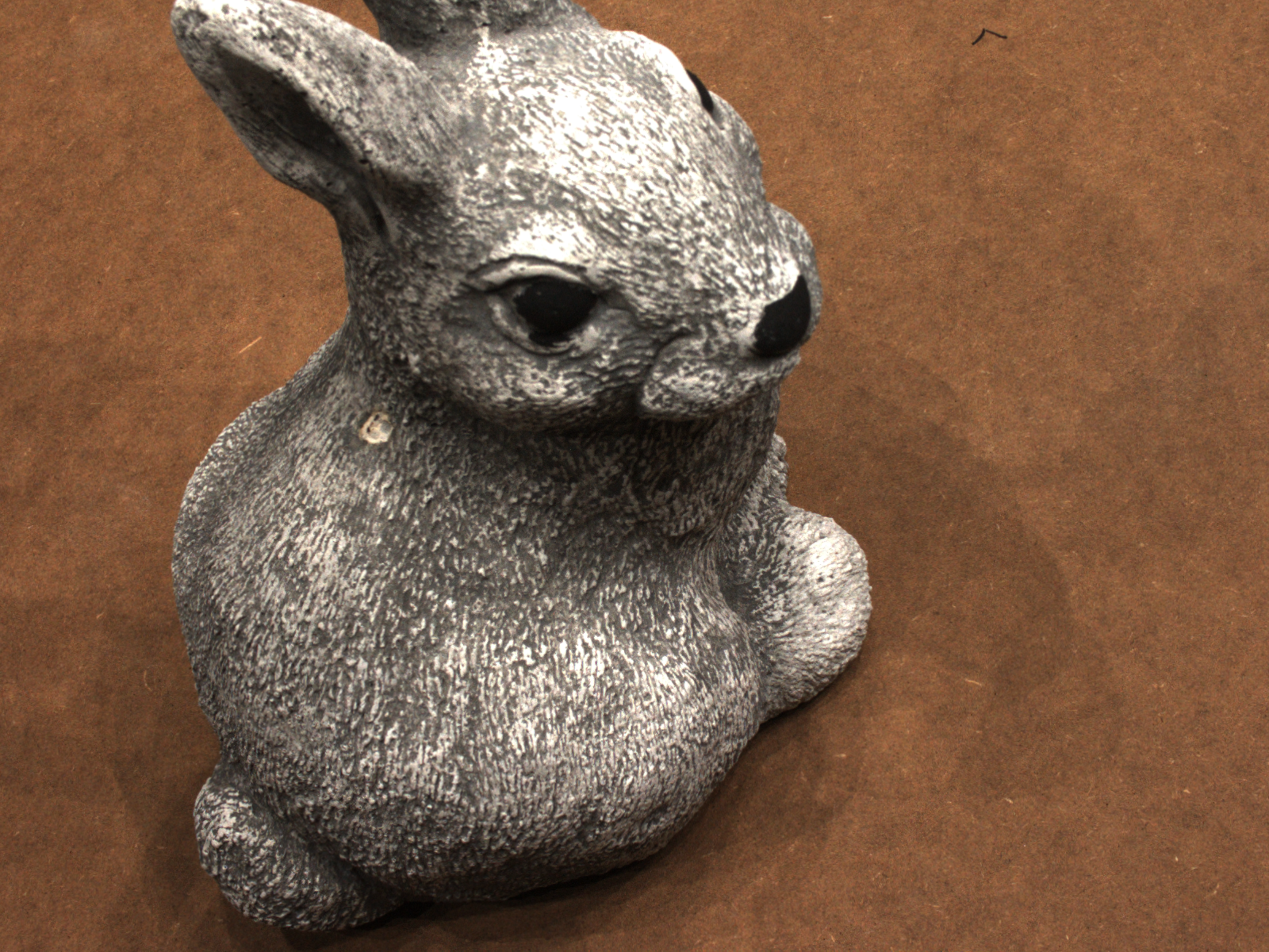
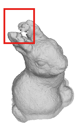
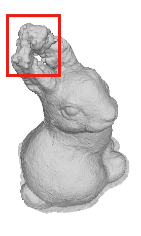
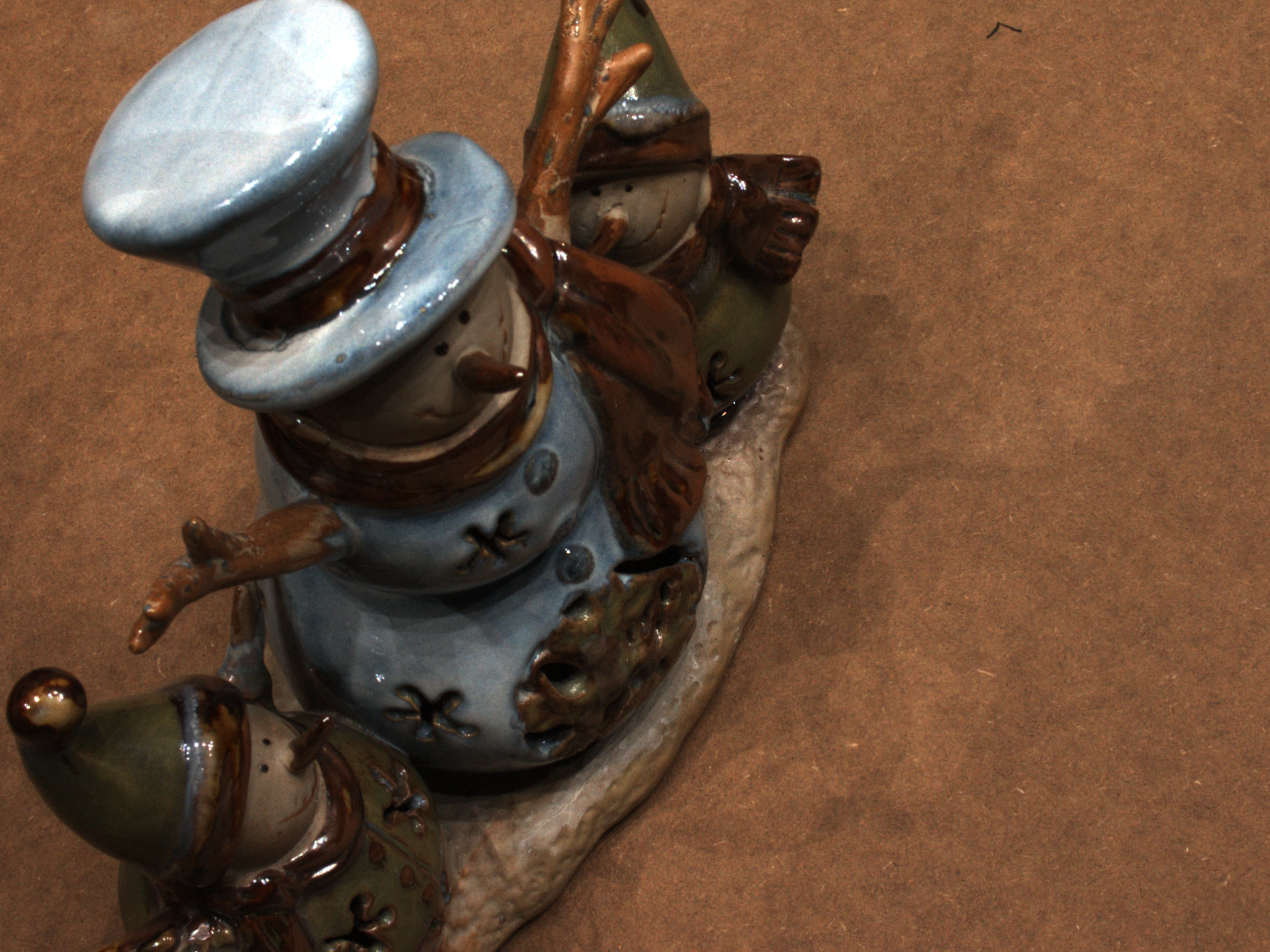
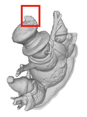
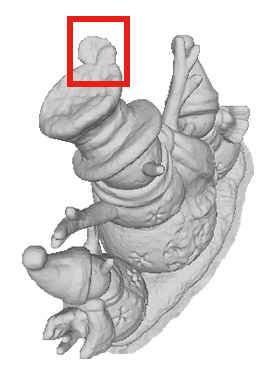
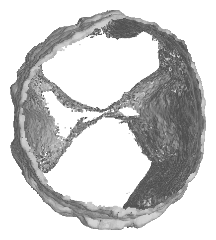
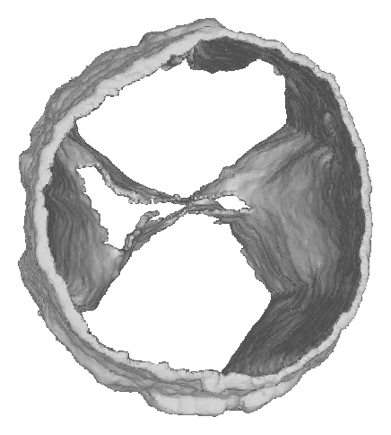
We compare the performance of NeUDF and HF-NeuS in reconstructing watertight models using the DTU dataset, which is known for its rich geometric details. The comparison focuses on the visual quality of the models’ output, specifically surface smoothness and the presence of artifacts. The DTU dataset poses challenges in 3D reconstruction due to the fact that many of the images only show a part of the object-of-interest. Despite this challenge, NeUDF is able to reconstruct watertight models with acceptable visual quality, especially in regions that are only visible in a few images. In comparison, HF-NeuS produces smoother surfaces than ours but introduces noticeable artifacts in regions with limited visibility. To illustrate the comparison, Figure 5 shows two examples of the output from both NeUDF and HF-NeuS on the DTU dataset.
| Reference Image | Ours | HF-NeuS |
|---|---|---|
 |
 |
 |
 |
 |
 |
4.3 Ablation Studies
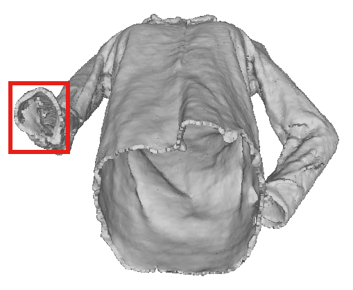
Regularization loss. The effectiveness of the iso-surface regularizer is verified through an ablation study. Figure 6 demonstrates that when trained with the regularization loss, the network successfully removes small and unwanted pieces, such as the parts covering the cuff of the sleeve in the reconstructed model. The iso-surface regularizer encourages clean and smooth UDFs, which reduces artifacts and produces a high-quality reconstructed model.
 |
 |
| w/ reg. | w/o reg. |
 |
 |
| w/ AHS | w/o AHS |
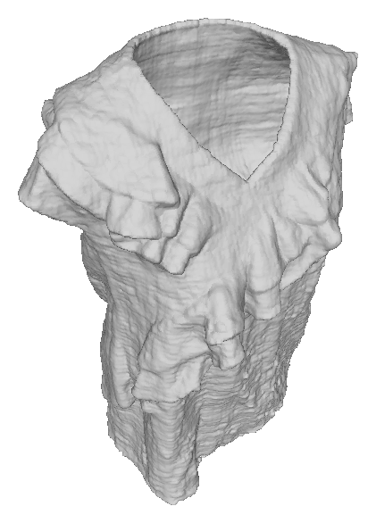
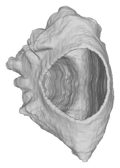
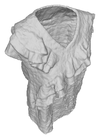
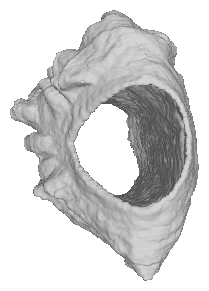
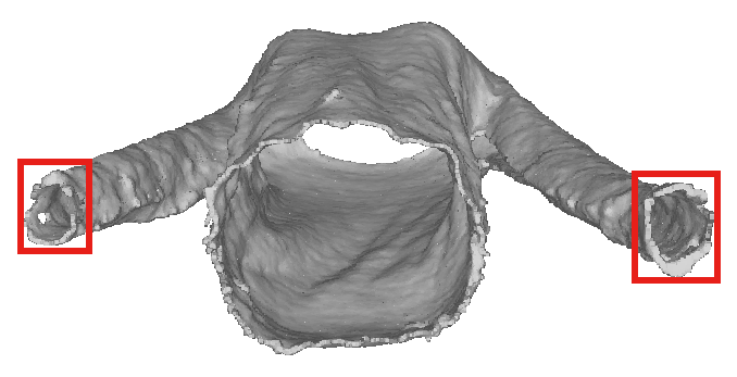
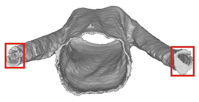
Adaptive hierarchical sampling. We train the model with and without AHS and compare their performance in terms of accuracy and visual quality. We found that using adaptive hierarchical upsampling helps to sample points more closely to the surface, especially for the parts close to boundaries, resulting in more accurate color computation in volume rendering. As shown in Figure 6, training with AHS produces better reconstruction on the sleeves.
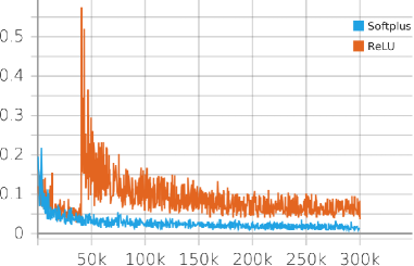
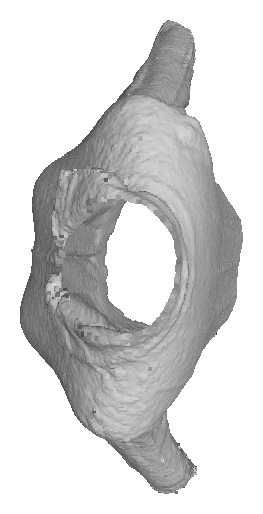
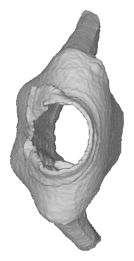
Non-negativity. Ensuring that the computed distances in the proposed method are non-negative is important, and can be achieved by applying either ReLU or softplus to the MLP output. However, ReLU is not differentiable at 0 and has vanishing gradients for negative inputs, which can make the network difficult to train. An ablation study confirms that training with ReLU only results in early progress, but fails to learn a valid UDF later on. See Figure 7 for details.
Extracting surface points. Instead of extracting the zero level-set from the learned UDFs, we construct the object surface by finding the points with the maximum weights. We compare our surface extraction method with MeshUDF [14], the state-of-the-art method for extracting the zero level-set from UDFs. Since our method is tailored to the proposed density function , it produces more accurate results than MeshUDF, which achieves the second best for most cases. See Table 1.
Limitations. Our method introduces a small bias during training, we can reduce the bias, but cannot eliminate it. Also, if the object has a very similar color to the background, our method has difficulty differentiating between the foreground object and the background, leading to incorrect result.
5 Conclusions
Overall, NeUDF offers a promising approach to the problem of reconstructing both open and watertight models from multi-view images. Its advantages over existing methods lie in the use of a simpler and more accurate density function, a smooth and differentiable UDF representation, and a simple yet effective surface reconstruction strategy tailored to the density function, which greatly improves the learning process. Results from our experiments on the DeepFashion3D and DTU datasets demonstrate the effectiveness of our method, particularly in reconstructing textureless models and regions with limited visibility. Moreover, our method does not rely on object masks, making it more practical in real-world applications.
In the future, we plan to investigate strictly unbiased and occlusion-aware density functions to fill the theoretical gap and further improve the accuracy of our method. We also aim to explore the use of sparse views for UDF learning.
References
- [1] Fausto Bernardini, Joshua Mittleman, Holly Rushmeier, Cláudio Silva, and Gabriel Taubin. The ball-pivoting algorithm for surface reconstruction. IEEE Transactions on Visualization and Computer Graphics, 5(4):349–359, oct 1999.
- [2] Jeremy S. De Bonet. Poxels: Probabilistic voxelized volume reconstruction. In Proc. Int. Conf. on Computer Vision (ICCV), 1999.
- [3] A. Broadhurst, T.W. Drummond, and R. Cipolla. A probabilistic framework for space carving. In Proceedings Eighth IEEE International Conference on Computer Vision. ICCV 2001, volume 1, pages 388–393 vol.1, 2001.
- [4] Rohan Chabra, Jan E. Lenssen, Eddy Ilg, Tanner Schmidt, Julian Straub, Steven Lovegrove, and Richard Newcombe. Deep local shapes: Learning local sdf priors for detailed 3d reconstruction. In Computer Vision – ECCV 2020: 16th European Conference, Glasgow, UK, August 23–28, 2020, Proceedings, Part XXIX, page 608–625, Berlin, Heidelberg, 2020. Springer-Verlag.
- [5] J. Chibane, T. Alldieck, and G. Pons-Moll. Implicit functions in feature space for 3d shape reconstruction and completion. In 2020 IEEE/CVF Conference on Computer Vision and Pattern Recognition (CVPR), pages 6968–6979, Los Alamitos, CA, USA, jun 2020. IEEE Computer Society.
- [6] Julian Chibane, Aymen Mir, and Gerard Pons-Moll. Neural unsigned distance fields for implicit function learning. In Proceedings of the 34th International Conference on Neural Information Processing Systems, NIPS’20, Red Hook, NY, USA, 2020. Curran Associates Inc.
- [7] François Darmon, Bénédicte Bascle, Jean-Clément Devaux, Pascal Monasse, and Mathieu Aubry. Improving neural implicit surfaces geometry with patch warping. In 2022 IEEE/CVF Conference on Computer Vision and Pattern Recognition (CVPR), pages 6250–6259, 2022.
- [8] Charles Dugas, Yoshua Bengio, François Bélisle, Claude Nadeau, and René Garcia. Incorporating second-order functional knowledge for better option pricing. In Proceedings of the 13th International Conference on Neural Information Processing Systems, NIPS’00, page 451–457, Cambridge, MA, USA, 2000. MIT Press.
- [9] Qiancheng Fu, Qingshan Xu, Yew-Soon Ong, and Wenbing Tao. Geo-neus: Geometry-consistent neural implicit surfaces learning for multi-view reconstruction. Advances in Neural Information Processing Systems (NeurIPS), 2022.
- [10] K Fukushima. Cognitron: a self-organizing multilayered neural network. Biological cybernetics, 20(3-4):121—136, November 1975.
- [11] Yasutaka Furukawa and Carlos Hernández. Multi-view stereo: A tutorial. Found. Trends. Comput. Graph. Vis., 9(1–2):1–148, jun 2015.
- [12] Silvano Galliani, Katrin Lasinger, and Konrad Schindler. Massively parallel multiview stereopsis by surface normal diffusion. In 2015 IEEE International Conference on Computer Vision (ICCV), pages 873–881, 2015.
- [13] Amos Gropp, Lior Yariv, Niv Haim, Matan Atzmon, and Yaron Lipman. Implicit geometric regularization for learning shapes. In ICML, volume 119, pages 3789–3799, 2020.
- [14] Benoit Guillard, Federico Stella, and Pascal Fua. Meshudf: Fast and differentiable meshing of unsigned distance field networks. In European Conference on Computer Vision, 2022.
- [15] Richard Hartley and Andrew Zisserman. Multiple View Geometry in Computer Vision. Cambridge University Press, 2 edition, 2004.
- [16] Fei Hou, Chiyu Wang, Wencheng Wang, Hong Qin, Chen Qian, and Ying He. Iterative poisson surface reconstruction (ipsr) for unoriented points. ACM Trans. Graph., 41(4), jul 2022.
- [17] Rasmus Jensen, Anders Dahl, George Vogiatzis, Engil Tola, and Henrik Aanæs. Large scale multi-view stereopsis evaluation. In 2014 IEEE Conference on Computer Vision and Pattern Recognition, pages 406–413, 2014.
- [18] Mengqi Ji, Jinzhi Zhang, Qionghai Dai, and Lu Fang. Surfacenet+: An end-to-end 3d neural network for very sparse multi-view stereopsis. IEEE Transactions on Pattern Analysis and Machine Intelligence, 43(11):4078–4093, 2021.
- [19] Abhishek Kar, Christian Häne, and Jitendra Malik. Learning a multi-view stereo machine. In Proceedings of the 31th International Conference on Neural Information Processing Systems, NIPS’17, page 364–375, Red Hook, NY, USA, 2017. Curran Associates Inc.
- [20] Michael Kazhdan and Hugues Hoppe. Screened poisson surface reconstruction. ACM Trans. Graph., 32(3), July 2013.
- [21] Diederik P. Kingma and Jimmy Ba. Adam: A method for stochastic optimization. In 3rd International Conference on Learning Representations, ICLR, San Diego, CA, USA, May 2015.
- [22] Xiaoxiao Long, Cheng Lin, Lingjie Liu, Yuan Liu, Peng Wang, Christian Theobalt, Taku Komura, and Wenping Wang. Neuraludf: Learning unsigned distance fields for multi-view reconstruction of surfaces with arbitrary topologies. ARXIV, 2022.
- [23] Xiaoxiao Long, Cheng Lin, Peng Wang, Taku Komura, and Wenping Wang. Sparseneus: Fast generalizable neural surface reconstruction from sparse views. In Computer Vision – ECCV 2022: 17th European Conference, Tel Aviv, Israel, October 23–27, 2022, Proceedings, Part XXXII, page 210–227, Berlin, Heidelberg, 2022. Springer-Verlag.
- [24] Baorui Ma, Zhizhong Han, Yu-Shen Liu, and Matthias Zwicker. Neural-pull: Learning signed distance function from point clouds by learning to pull space onto surface. In Marina Meila and Tong Zhang, editors, Proceedings of the 38th International Conference on Machine Learning, ICML 2021, 18-24 July 2021, Virtual Event, volume 139 of Proceedings of Machine Learning Research, pages 7246–7257. PMLR, 2021.
- [25] N. Max. Optical models for direct volume rendering. IEEE Transactions on Visualization and Computer Graphics, 1(2):99–108, 1995.
- [26] Lars Mescheder, Michael Oechsle, Michael Niemeyer, Sebastian Nowozin, and Andreas Geiger. Occupancy networks: Learning 3d reconstruction in function space. In 2019 IEEE/CVF Conference on Computer Vision and Pattern Recognition (CVPR), pages 4455–4465, 2019.
- [27] Ben Mildenhall, Pratul P. Srinivasan, Matthew Tancik, Jonathan T. Barron, Ravi Ramamoorthi, and Ren Ng. Nerf: Representing scenes as neural radiance fields for view synthesis. In European Conference on Computer Vision, 2020.
- [28] Jeong Joon Park, Peter R. Florence, Julian Straub, Richard A. Newcombe, and S. Lovegrove. Deepsdf: Learning continuous signed distance functions for shape representation. 2019 IEEE/CVF Conference on Computer Vision and Pattern Recognition (CVPR), pages 165–174, 2019.
- [29] Keunhong Park, Utkarsh Sinha, Jonathan T. Barron, Sofien Bouaziz, Dan B Goldman, Steven M. Seitz, and Ricardo Martin-Brualla. Nerfies: Deformable neural radiance fields. ICCV, 2021.
- [30] Johannes L. Schönberger, Enliang Zheng, Jan-Michael Frahm, and Marc Pollefeys. Pixelwise view selection for unstructured multi-view stereo. In Bastian Leibe, Jiri Matas, Nicu Sebe, and Max Welling, editors, Computer Vision – ECCV 2016, pages 501–518, Cham, 2016. Springer International Publishing.
- [31] Vincent Sitzmann, Julien N. P. Martel, Alexander W. Bergman, David B. Lindell, and Gordon Wetzstein. Implicit neural representations with periodic activation functions. In Proceedings of the 34th International Conference on Neural Information Processing Systems, NIPS’20, Red Hook, NY, USA, 2020. Curran Associates Inc.
- [32] J. Sun, Y. Xie, L. Chen, X. Zhou, and H. Bao. Neuralrecon: Real-time coherent 3d reconstruction from monocular video. In 2021 IEEE/CVF Conference on Computer Vision and Pattern Recognition (CVPR), pages 15593–15602, Los Alamitos, CA, USA, jun 2021. IEEE Computer Society.
- [33] Peng Wang, Lingjie Liu, Yuan Liu, Christian Theobalt, Taku Komura, and Wenping Wang. Neus: Learning neural implicit surfaces by volume rendering for multi-view reconstruction. In Advances in Neural Information Processing Systems 34: Annual Conference on Neural Information Processing Systems 2021, NeurIPS 2021, December 6-14, 2021, virtual, pages 27171–27183, 2021.
- [34] Yifan Wang, Lukas Rahmann, and Olga Sorkine-Hornung. Geometry-consistent neural shape representation with implicit displacement fields. In The Tenth International Conference on Learning Representations, ICLR 2022, Virtual Event, April 25-29, 2022. OpenReview.net, 2022.
- [35] Yiqun Wang, Ivan Skorokhodov, and Peter Wonka. Hf-neus: Improved surface reconstruction using high-frequency details. In Proceedings of the 36th International Conference on Neural Information Processing Systems, 2022.
- [36] Y. Yao, Z. Luo, S. Li, T. Shen, T. Fang, and L. Quan. Recurrent mvsnet for high-resolution multi-view stereo depth inference. In 2019 IEEE/CVF Conference on Computer Vision and Pattern Recognition (CVPR), pages 5520–5529, Los Alamitos, CA, USA, jun 2019. IEEE Computer Society.
- [37] Lior Yariv, Jiatao Gu, Yoni Kasten, and Yaron Lipman. Volume rendering of neural implicit surfaces. In Thirty-Fifth Conference on Neural Information Processing Systems, 2021.
- [38] Kai Zhang, Gernot Riegler, Noah Snavely, and Vladlen Koltun. Nerf++: Analyzing and improving neural radiance fields. arXiv:2010.07492, 2020.
- [39] F. Zhao, W. Wang, S. Liao, and L. Shao. Learning anchored unsigned distance functions with gradient direction alignment for single-view garment reconstruction. In 2021 IEEE/CVF International Conference on Computer Vision (ICCV), pages 12654–12663, Los Alamitos, CA, USA, oct 2021. IEEE Computer Society.
- [40] Junsheng Zhou, Baorui Ma, Liu Yu-Shen, Fang Yi, and Han Zhizhong. Learning consistency-aware unsigned distance functions progressively from raw point clouds. In Advances in Neural Information Processing Systems (NeurIPS), 2022.
- [41] Heming Zhu, Yu Cao, Hang Jin, Weikai Chen, Dong Du, Zhangye Wang, Shuguang Cui, and Xiaoguang Han. Deep fashion3d: A dataset and benchmark for 3d garment reconstruction from single images. In Andrea Vedaldi, Horst Bischof, Thomas Brox, and Jan-Michael Frahm, editors, Computer Vision – ECCV 2020, pages 512–530, Cham, 2020. Springer International Publishing.
6 Supplementary Material
6.1 More Results
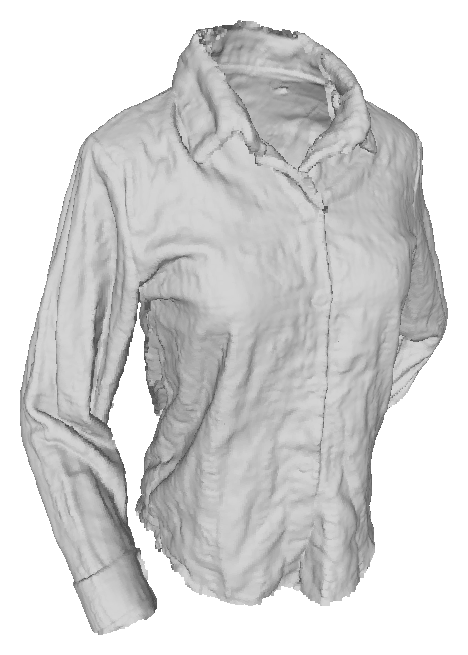
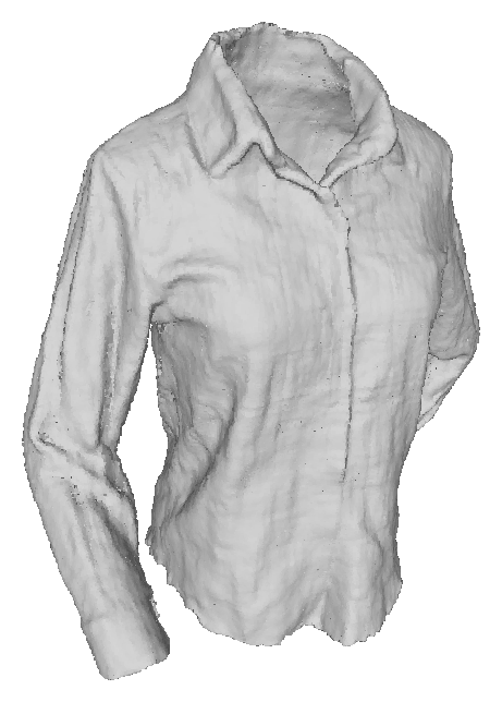
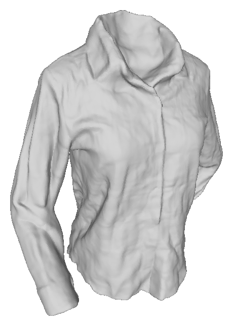
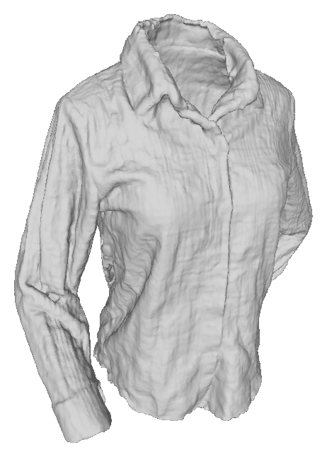
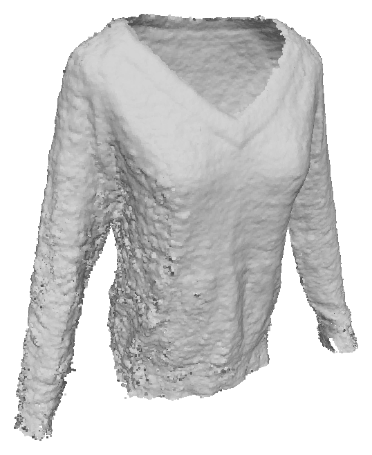
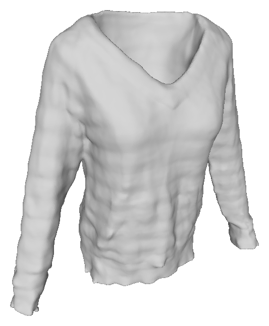
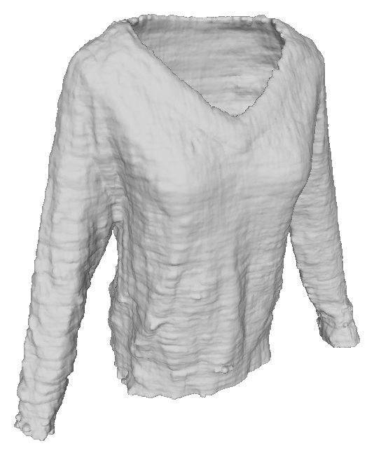
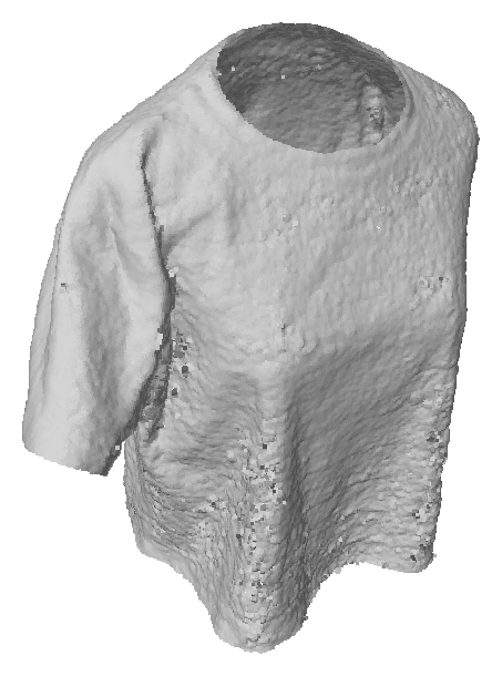
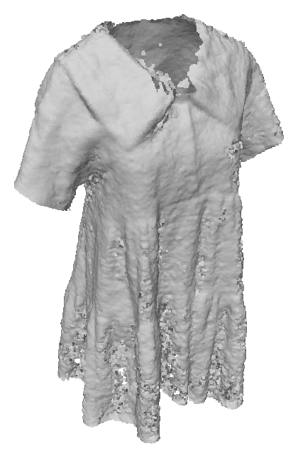
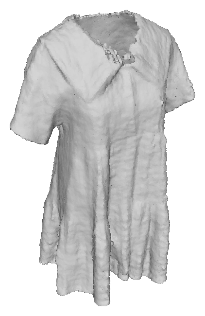
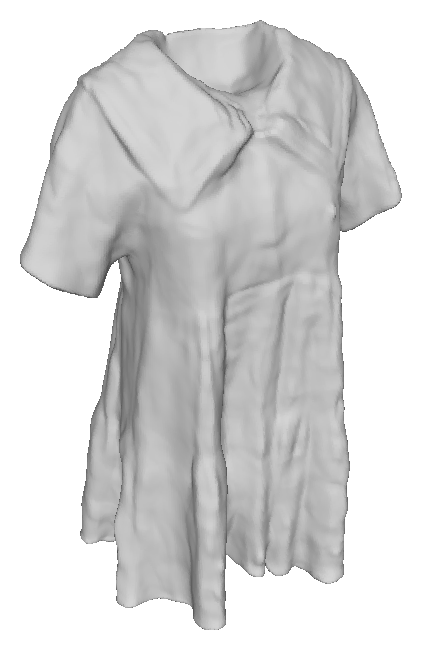
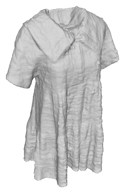
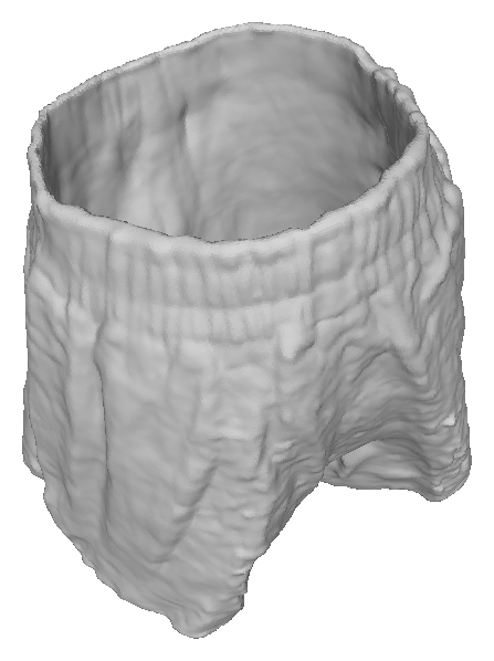
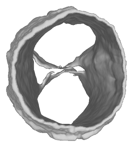
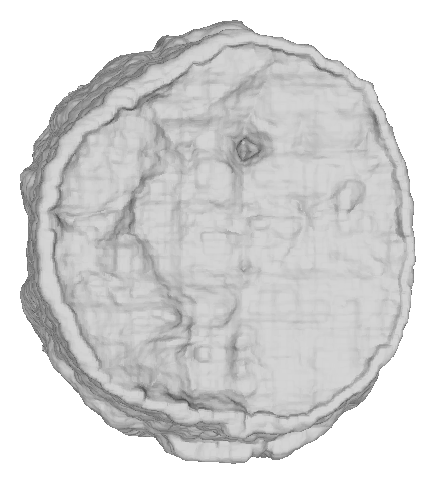
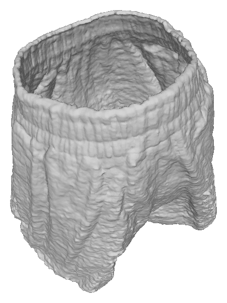
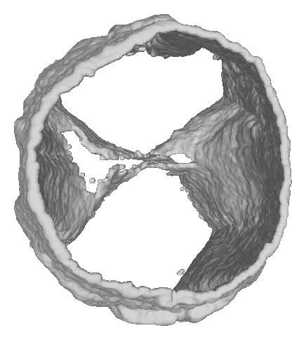
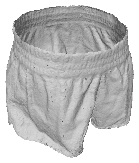
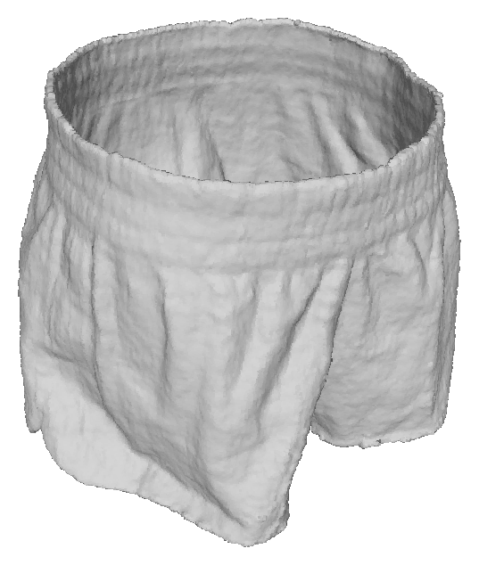
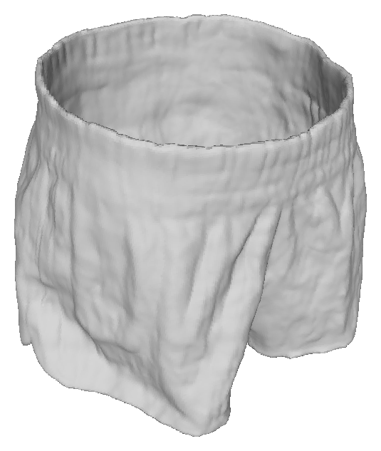
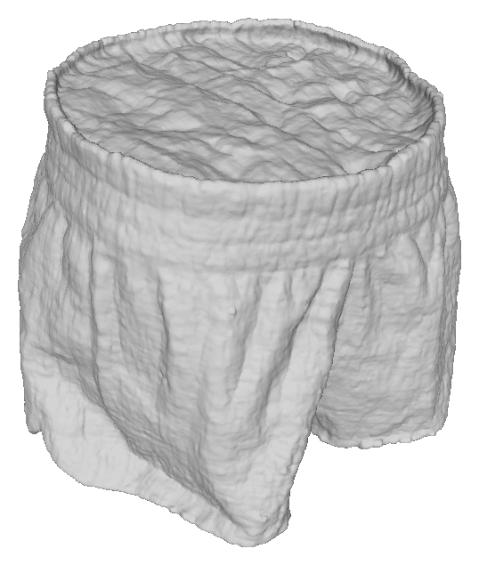
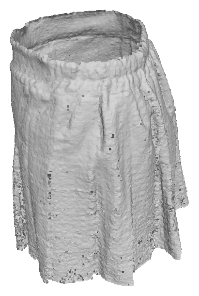
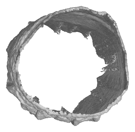
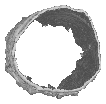
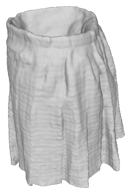
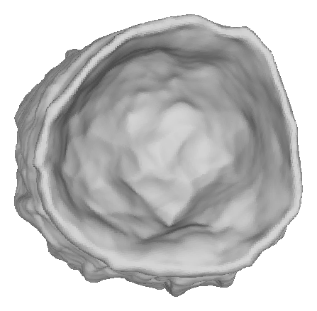
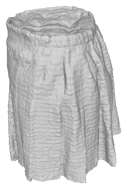
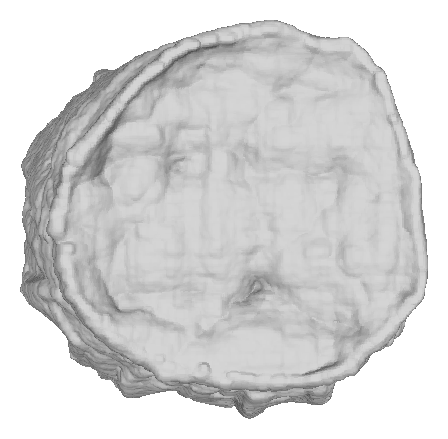
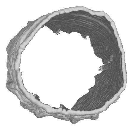
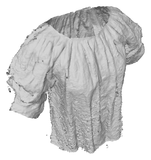
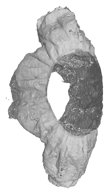
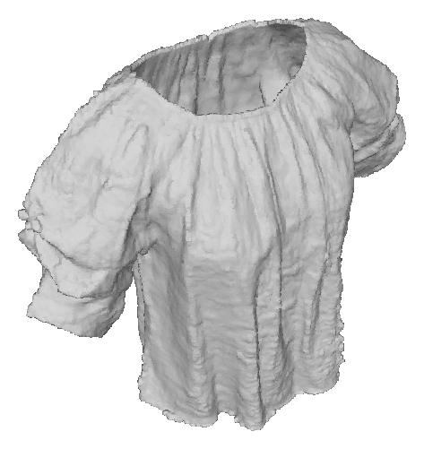
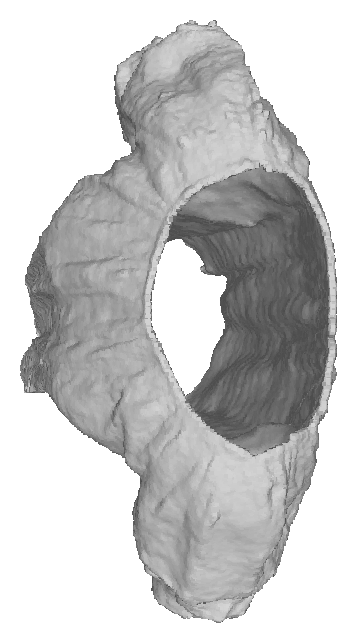
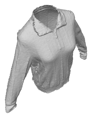
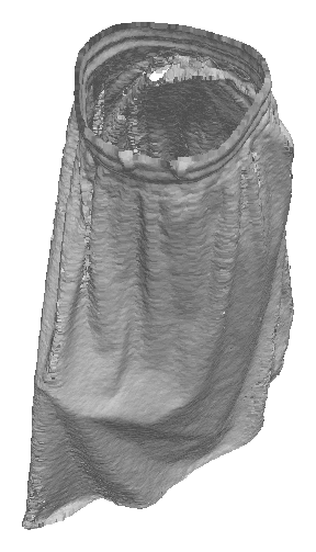
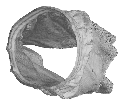
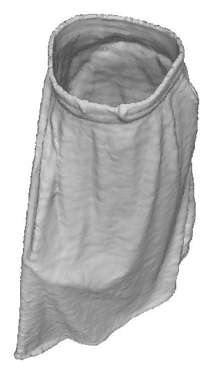
We present the remaining results on DeepFashion3D [41] dataset in Figure 8. They have various textures. We consider models having mostly pure color, or without highly contrasting colors to be textureless. Hence, #7, #8 and #9 are textureless, models #2 and #11 are with grid textures, models #3 and #4 are with stripe textures, and models #10 and #12 are with fancy textures.
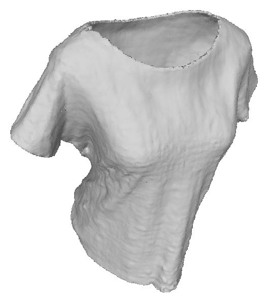
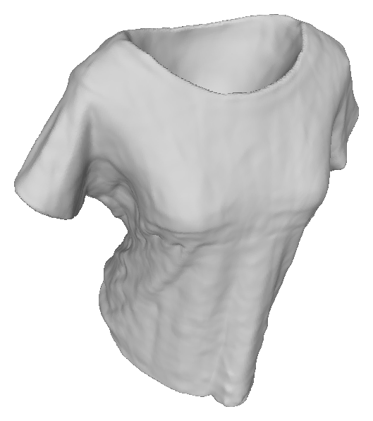
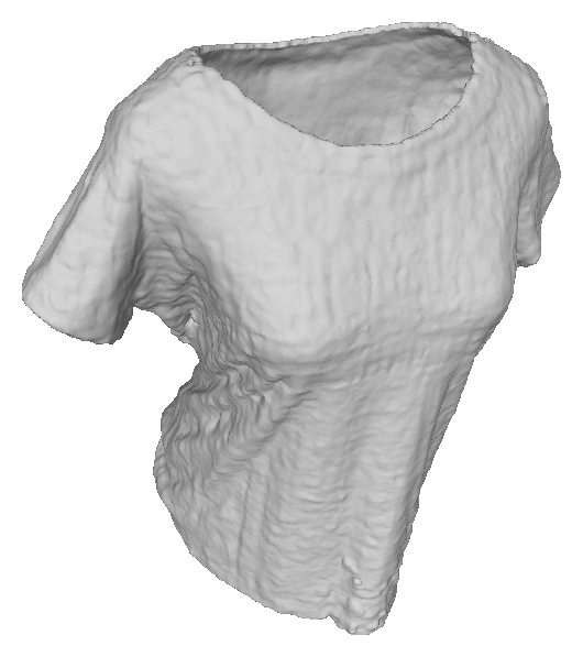
We also generate three more results of challenge textureless models, as shown in Figure 9.
| Reference Image | GT | Ours | VolSDF [37] | NeuS [33] | HF-NeuS [35] | |
|---|---|---|---|---|---|---|
| #2 | 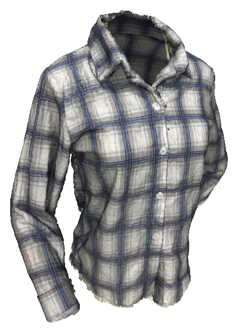 |
 |
 |
 |
 |
 |
| #3 | 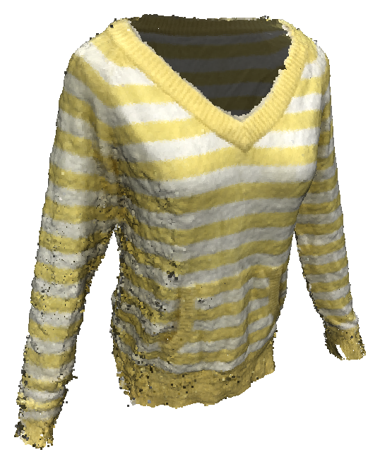 |
 |
 |
 |
 |
 |
| #4 | 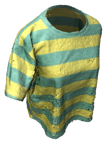 |
 |
 |
 |
 |
 |
| #7 | 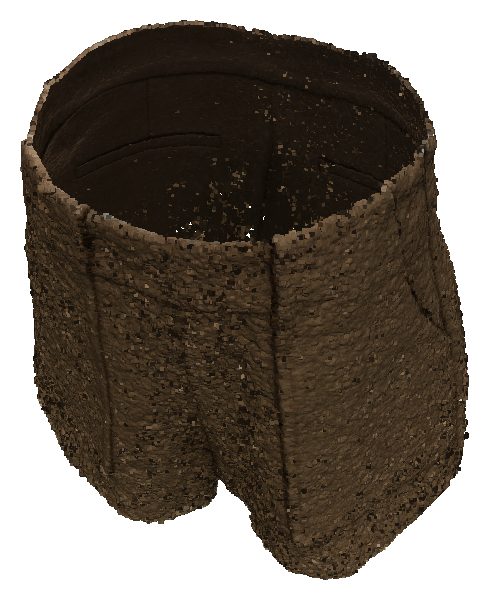 |
 |
 |
 |
 |
 |
| #8 | 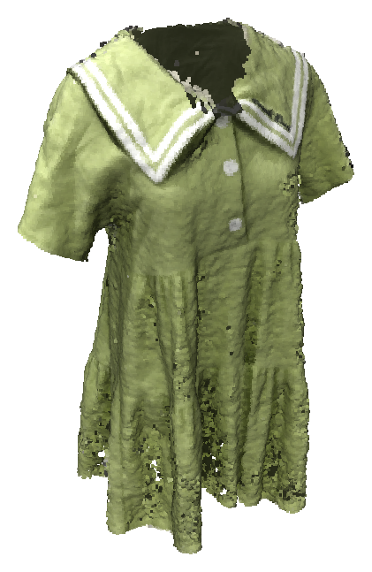 |
 |
 |
 |
 |
 |
| #9 |  |
|
|
|
|
|
| #10 | 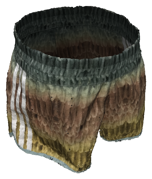 |
 |
 |
 |
 |
 |
| #11 | 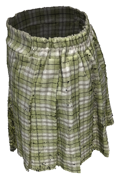 |
|
|
|
|
|
| #12 | 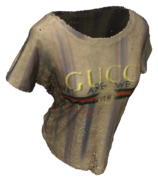 |
 |
 |
 |
 |
 |
| Reference Image | GT | Ours | |
| #13 | 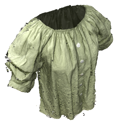 |
|
|
|---|---|---|---|
| CD | |||
| #14 | 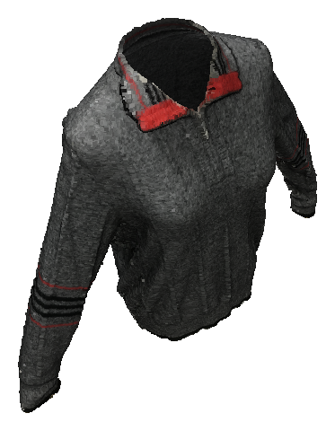 |
|
|
| CD | |||
| #15 | 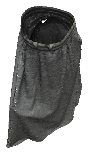 |
|
|
| CD |