Low-Complexity Memory AMP Detector for High-Mobility MIMO-OTFS SCMA Systems

Yao Ge1, Lei Liu2, Shunqi Huang2, David González G.3, Yong Liang Guan1, and Zhi Ding4 1Continental-NTU Corporate Lab, Nanyang Technological University, Singapore 2School of Information Science, Japan Institute of Science and Technology (JAIST), Nomi 923-1292, Japan 3Wireless Communications Technologies Group, Continental AG, Germany 4Department of Electrical and Computer Engineering, University of California at Davis, Davis, CA 95616 USA Emails: 1{yao.ge;eylguan}@ntu.edu.sg, 2{leiliu;shunqi.huang}@jaist.ac.jp, 3david.gonzalez.g@ieee.org, 4zding@ucdavis.edu
Abstract

Efficient signal detectors are rather important yet challenging to achieve satisfactory performance for large-scale communication systems. This paper considers a non-orthogonal sparse code multiple access (SCMA) configuration for multiple-input multiple-output (MIMO) systems with recently proposed orthogonal time frequency space (OTFS) modulation. We develop a novel low-complexity yet effective customized Memory approximate message passing (AMP) algorithm for channel equalization and multi-user detection. Specifically, the proposed Memory AMP detector enjoys the sparsity of the channel matrix and only applies matrix-vector multiplications in each iteration for low-complexity. To alleviate the performance degradation caused by positive reinforcement problem in the iterative process, all the preceding messages are utilized to guarantee the orthogonality principle in Memory AMP detector. Simulation results are finally provided to illustrate the superiority of our Memory AMP detector over the existing solutions.

Index Terms:
AMP, high-mobility communications, MIMO, OTFS, SCMA.

I Introduction

The orthogonal time frequency space (OTFS) modulation [1] has emerged as a promising and alternative modulation scheme to traditional orthogonal frequency-division multiplexing (OFDM) for high mobility communications. Unlike OFDM, OTFS multiplexes information symbols in the delay-Doppler domain and exploits the diversity coming from both the channel delays and Doppler shifts for better performance. Thanks to the sparsity of the channel in delay-Doppler domain, the required pilot and receiver complexity for channel estimation can be significantly reduced [2]. However, the equivalent transmission of OTFS in the delay-Doppler domain involves a sophisticated two-dimensional periodic convolution, leading to severe inter-symbol interference (ISI) [3]. Therefore, simple and effective signal detectors are rather important for OTFS systems to maintain the sufficient diversity of the wireless channel and achieve desired receiver performance.

In addition, multiple-input multiple-output (MIMO) can be combined with OTFS to further increase spectral efficiency and transmission reliability for high mobility scenarios [4, 5, 6]. Meanwhile, non-orthogonal multiple access (NOMA) has been integrated with OTFS to improve spectrum utilization and massive user connectivity [7, 8]. In OTFS-NOMA, multiple users are allowed to access the same delay-Doppler resources simultaneously, and distinguished by different power levels [7] or via sparse code multiple access (SCMA) [8]. However, a major challenge for MIMO-OTFS multi-user systems is the data detection at the receiver due to the substantial increase of system dimension and the additional inter-user interference, which requires complicated processing with high complexity.

The optimal maximum a posteriori (MAP) detector is impractical due to its complexity growing exponentially with the system dimension. The existing linear detectors such as zero-forcing (ZF) and linear minimum mean square error (LMMSE) [4] leading to severe performance loss. Recently, several studies [9, 5, 6] exploit the typical structure and characteristic of OTFS transmission matrix for interference cancellation and performance improvement. Unfortunately, the typical OTFS channel matrix structures do not always hold and the interference cancellation may cause error propagation. By leveraging the sparsity of OTFS channel matrix, the efficient Gaussian message passing (GMP) [10, 11] and expectation propagation (EP) [8, 12] detectors are developed with low-complexity. However, the GMP and EP detectors may suffer from performance loss if so many short girths (i.e., girth-4) exist in the factor graph. Alternatively, orthogonal/vector approximate message passing (OAMP/VAMP) [7] are proposed for OTFS systems with more robustness performance. However, the high computational cost caused by either matrix inverse or singular-value decomposition (SVD) of OAMP/VAMP limits their applications to large-scale systems.

Recently, a Bayesian inference technique denoted as Memory approximate message passing (AMP) [13] was proposed for sparse signal recovery with performance improvement. Inspired by [13], we develop an efficient customized Memory AMP detector for MIMO-OTFS SCMA systems, where the typical sparse channel matrix is applied to further reduce the complexity. Our Memory AMP detector only involves a low-complexity matched filter in each iteration, and applies finite terms of matrix Taylor series to approximate the matrix inverse. Based on the specific orthogonality principle and closed-form damping solution, our proposed Memory AMP detector outperforms the heuristic damping-based GMP and EP detectors, and achieves similar performance to that of OAMP/VAMP but with low-complexity.

II System Model

We consider an uplink MIMO-OTFS SCMA system with J𝐽J independent mobile users transmitting signals to the base station (BS) simultaneously. Without loss of generality, each user is equipped with one transmit antenna and the BS is equipped with U𝑈U receive antennas. At each transmit slot, every log2Qsubscript2𝑄{\log_{2}}Q information bits 𝐛jsubscript𝐛𝑗{{\bf{b}}_{j}} from the j𝑗j-th user are mapped into a K𝐾K-dimensional sparse codeword 𝐜j=[cj1,cj2,,cjK]Tsubscript𝐜𝑗superscriptsuperscriptsubscript𝑐𝑗1superscriptsubscript𝑐𝑗2superscriptsubscript𝑐𝑗𝐾𝑇{{\bf{c}}_{j}}={\left[{c_{j}^{1},c_{j}^{2},\cdots,c_{j}^{K}}\right]^{T}} selected from a user-specific SCMA codebook 𝔸jsubscript𝔸𝑗\mathbb{A}_{j} of size Q𝑄Q, where j={1,2,,J}𝑗12𝐽j=\{1,2,\cdots,J\} and J>K𝐽𝐾J>K typically, leading to an overloading factor ζ=JK>1𝜁𝐽𝐾1\zeta=\frac{J}{K}>1. We assume that each user employs only one SCMA layer and only D𝐷D (D<K𝐷𝐾D<K) non-zero entries among the K𝐾K-dimensional codeword 𝐜jsubscript𝐜𝑗{{\bf{c}}_{j}}. We then generate the information symbols in the delay-Doppler plane 𝐗jM×Nsubscript𝐗𝑗superscript𝑀𝑁{\bf{X}}_{j}\in{\mathbb{C}^{M\times N}} of the j𝑗j-th user by allocating MNK𝑀𝑁𝐾\frac{{MN}}{K} SCMA codewords 𝐜jsubscript𝐜𝑗{{\bf{c}}_{j}} either along the delay axis or along the Doppler axis without overlapping. Here, M𝑀M and N𝑁N are numbers of resource grids along the delay and Doppler dimensions, respectively.111For simplicity, we assume that M𝑀M and N𝑁N are integer multiples of K𝐾K, i.e., [M]K=[N]K=0subscriptdelimited-[]𝑀𝐾subscriptdelimited-[]𝑁𝐾0{[M]_{K}}={[N]_{K}}=0, where []ksubscriptdelimited-[]𝑘{\left[\cdot\right]_{k}} denotes mod-k𝑘k operation. The transmission scheme for each user is based on OTFS to combat the doubly-selective fading channels caused by channel delays and Doppler shifts.

Specifically, the transmitted time domain signal in OTFS can be obtained by first applying the inverse symplectic finite Fourier transform (ISFFT) on 𝐗jM×Nsubscript𝐗𝑗superscript𝑀𝑁{\bf{X}}_{j}\in{\mathbb{C}^{M\times N}} followed by Heisenberg transform. Assuming rectangular transmit pulse, the output of the Heisenberg transform can be given by

𝐒j=𝐅MH(𝐅M𝐗j𝐅NH)=𝐗j𝐅NH,subscript𝐒𝑗superscriptsubscript𝐅𝑀𝐻subscript𝐅𝑀subscript𝐗𝑗superscriptsubscript𝐅𝑁𝐻subscript𝐗𝑗superscriptsubscript𝐅𝑁𝐻\displaystyle{\bf{S}}_{j}={\bf{F}}_{M}^{H}({{\bf{F}}_{M}}{\bf{X}}_{j}{\bf{F}}_{N}^{H})={\bf{X}}_{j}{\bf{F}}_{N}^{H}, (1)

where 𝐅MM×Msubscript𝐅𝑀superscript𝑀𝑀{{\bf{F}}_{M}}\in{\mathbb{C}^{M\times M}} and 𝐅NN×Nsubscript𝐅𝑁superscript𝑁𝑁{{\bf{F}}_{N}}\in{\mathbb{C}^{N\times N}} represent normalized M𝑀M-point and N𝑁N-point fast Fourier transform (FFT) matrices, respectively. The transmitted time domain signal 𝐬jMN×1subscript𝐬𝑗superscript𝑀𝑁1{\bf{s}}_{j}\in{\mathbb{C}^{MN\times 1}} can be generated by column-wise vectorization of 𝐒jsubscript𝐒𝑗{\bf{S}}_{j}.

We then add a cyclic prefix (CP) in front of the generated time domain signal for each user. After passing through a transmit filter, the resulted time domain signal of each user is sent out simultaneously over the doubly-selective fading channels. Here, we characterize the impulse response channel between j𝑗j-th user and u𝑢u-th receive antenna as

huj[c,p]=subscript𝑢𝑗𝑐𝑝absent\displaystyle{h_{uj}}\left[{c,p}\right]= i=1Lujhuj,iej2πνuj,i(cTspTs)Prc(pTstjτuj,i),superscriptsubscript𝑖1subscript𝐿𝑢𝑗subscript𝑢𝑗𝑖superscript𝑒𝑗2𝜋subscript𝜈𝑢𝑗𝑖𝑐subscript𝑇𝑠𝑝subscript𝑇𝑠subscriptPrc𝑝subscript𝑇𝑠subscript𝑡𝑗subscript𝜏𝑢𝑗𝑖\displaystyle\sum\limits_{i=1}^{L_{uj}}{{h_{uj,i}}{e^{j2\pi{\nu_{uj,i}}\left({c{T_{s}}-p{T_{s}}}\right)}}{{\mathop{\rm P}\nolimits}_{\text{{rc}}}}(p{T_{s}}-{t_{j}}-{\tau_{uj,i}})},
c=0,,MN1;p=0,,Puj1,formulae-sequence𝑐0𝑀𝑁1𝑝0subscript𝑃𝑢𝑗1\displaystyle c=0,\cdots,MN-1;\;p=0,\cdots,P_{uj}-1, (2)

where Lujsubscript𝐿𝑢𝑗{L_{uj}} is the number of multipaths between the j𝑗j-th user and the u𝑢u-th receive antenna, and tjsubscript𝑡𝑗{t_{j}} denotes the timing offset experienced by the j𝑗j-th user; huj,isubscript𝑢𝑗𝑖h_{uj,i}, τuj,isubscript𝜏𝑢𝑗𝑖\tau_{uj,i} and νuj,isubscript𝜈𝑢𝑗𝑖\nu_{uj,i} represent the channel gain, delay and Doppler frequency shift associated with the i𝑖i-th path, respectively. The system sampling interval Ts=1/MΔfsubscript𝑇𝑠1/𝑀Δ𝑓{T_{s}}={1\mathord{\left/{\vphantom{1{M\Delta f}}}\right.\kern-1.2pt}{M\Delta f}}. The Doppler frequency shift νuj,isubscript𝜈𝑢𝑗𝑖\nu_{uj,i} can be further expressed as νuj,i=(kuj,i+βuj,i)/NTsubscript𝜈𝑢𝑗𝑖subscript𝑘𝑢𝑗𝑖subscript𝛽𝑢𝑗𝑖𝑁𝑇\nu_{uj,i}=({{k_{{uj,i}}}+{\beta_{{uj,i}}}})/NT, where integer kuj,isubscript𝑘𝑢𝑗𝑖{{k_{{uj,i}}}} and real βuj,i(0.5,0.5]subscript𝛽𝑢𝑗𝑖0.50.5{\beta_{{uj,i}}}\in\left({-0.5,0.5}\right] respectively stand for the index and fractional part of νuj,isubscript𝜈𝑢𝑗𝑖\nu_{uj,i}. T𝑇T (seconds) and Δf=1/TΔ𝑓1/𝑇\Delta f={1\mathord{\left/{\vphantom{1T}}\right.\kern-1.2pt}T} (Hz) are chosen to be larger than the maximal channel delay spread and maximum Doppler frequency shift, respectively.

In (II), Prc()subscriptPrc{{{\mathop{\rm P}\nolimits}_{\text{{rc}}}}(\cdot)} is an equivalent overall raised-cosine (RC) rolloff filter when the typical root raised-cosine (RRC) pulse shaping filters are applied at the transmitter and receiver. The maximal channel tap Pujsubscript𝑃𝑢𝑗P_{uj} is determined by the duration of the overall filter response and the maximum channel delay spread. To overcome the inter-frame interference, we append a CP which is sufficiently long to accommodate both the maximum timing offset and maximal channel delay spread of all users.

The received time domain signal first enters a received filter. After discarding the CP, we can express the received signal from the j𝑗j-th user at the u𝑢u-th receive antenna as

ruj[c]=p=0Puj1huj[c,p]sj[[cp]MN],c=0,,MN1.formulae-sequencesubscript𝑟𝑢𝑗delimited-[]𝑐superscriptsubscript𝑝0subscript𝑃𝑢𝑗1subscript𝑢𝑗𝑐𝑝subscript𝑠𝑗delimited-[]subscriptdelimited-[]𝑐𝑝𝑀𝑁𝑐0𝑀𝑁1\displaystyle r_{uj}[c]=\sum\limits_{p=0}^{P_{uj}-1}{h_{uj}[c,p]s_{j}\left[{{{\left[{c-p}\right]}_{MN}}}\right]},\;c=0,\cdots,MN-1.

The resulting signal 𝐫ujMN×1subscript𝐫𝑢𝑗superscript𝑀𝑁1{\bf{r}}_{uj}\in{\mathbb{C}^{MN\times 1}} is then devectorized into a matrix 𝐑ujM×Nsubscript𝐑𝑢𝑗superscript𝑀𝑁{\bf{R}}_{uj}\in{\mathbb{C}^{M\times N}}, followed by Wigner transform as well as the symplectic finite Fourier transform (SFFT), yielding

𝐘uj=𝐅MH(𝐅M𝐑uj)𝐅N=𝐑uj𝐅N.subscript𝐘𝑢𝑗superscriptsubscript𝐅𝑀𝐻subscript𝐅𝑀subscript𝐑𝑢𝑗subscript𝐅𝑁subscript𝐑𝑢𝑗subscript𝐅𝑁\displaystyle{\bf{Y}}_{uj}={\bf{F}}_{M}^{H}({{\bf{F}}_{M}}{\bf{R}}_{uj}){\bf{F}}_{N}={\bf{R}}_{uj}{\bf{F}}_{N}. (3)

Finally, the end-to-end delay-Doppler domain input-output model from j𝑗j-th user to u𝑢u-th receive antenna is given by [3]

Yuj[,k]=p=0Puj1i=1Lujq=0N1huj,iPrc(pTstjτuj,i)subscript𝑌𝑢𝑗𝑘superscriptsubscript𝑝0subscript𝑃𝑢𝑗1superscriptsubscript𝑖1subscript𝐿𝑢𝑗superscriptsubscript𝑞0𝑁1subscript𝑢𝑗𝑖subscriptPrc𝑝subscript𝑇𝑠subscript𝑡𝑗subscript𝜏𝑢𝑗𝑖\displaystyle Y_{uj}[\ell,k]=\sum\limits_{p=0}^{P_{uj}-1}{\sum\limits_{i=1}^{L_{uj}}{\sum\limits_{q=0}^{N-1}{{h_{uj,i}}{{\mathop{\rm P}\nolimits}_{\text{{rc}}}}(p{T_{s}}-{t_{j}}-{\tau_{uj,i}})}}}
×\displaystyle\times γ(k,,p,q,kuj,i,βuj,i)Xj[[p]M,[kkuj,i+q]N],𝛾𝑘𝑝𝑞subscript𝑘𝑢𝑗𝑖subscript𝛽𝑢𝑗𝑖subscript𝑋𝑗subscriptdelimited-[]𝑝𝑀subscriptdelimited-[]𝑘subscript𝑘𝑢𝑗𝑖𝑞𝑁\displaystyle\gamma(k,\ell,p,q,{k_{{uj,i}}},{\beta_{{uj,i}}})X_{j}[{{{[{\ell-p}]}_{M}},{{[{k-{k_{{uj,i}}}+q}]}_{N}}}], (4)

where

γ(k,,p,q,kuj,i,βuj,i)𝛾𝑘𝑝𝑞subscript𝑘𝑢𝑗𝑖subscript𝛽𝑢𝑗𝑖\displaystyle\gamma(k,\ell,p,q,{k_{{uj,i}}},{\beta_{{uj,i}}}) (5a)
={1Nξ(,p,kuj,i,βuj,i)θ(q,βuj,i),p<M,1Nξ(,p,kuj,i,βuj,i)θ(q,βuj,i)ϕ(k,q,kuj,i),0<p,absentcases1𝑁𝜉𝑝subscript𝑘𝑢𝑗𝑖subscript𝛽𝑢𝑗𝑖𝜃𝑞subscript𝛽𝑢𝑗𝑖𝑝𝑀1𝑁𝜉𝑝subscript𝑘𝑢𝑗𝑖subscript𝛽𝑢𝑗𝑖𝜃𝑞subscript𝛽𝑢𝑗𝑖italic-ϕ𝑘𝑞subscript𝑘𝑢𝑗𝑖0𝑝\displaystyle=\!\begin{cases}\frac{1}{N}\xi(\ell,p,{k_{{uj,i}}},{\beta_{{uj,i}}})\theta(q,{\beta_{{uj,i}}}),\!\!&p\!\leq\!\ell\!<\!M,\\ \frac{1}{N}\xi(\ell,p,{k_{{uj,i}}},{\beta_{{uj,i}}})\theta(q,{\beta_{{uj,i}}})\phi(k,q,{k_{{uj,i}}}),\!&0\!\leq\!\ell\!<\!p,\end{cases}
ξ(,p,kuj,i,βuj,i)=ej2π(pM)(kuj,i+βuj,iN),𝜉𝑝subscript𝑘𝑢𝑗𝑖subscript𝛽𝑢𝑗𝑖superscript𝑒𝑗2𝜋𝑝𝑀subscript𝑘𝑢𝑗𝑖subscript𝛽𝑢𝑗𝑖𝑁\displaystyle\xi(\ell,p,{k_{{uj,i}}},{\beta_{{uj,i}}})={e^{j2\pi\left({\frac{{\ell-p}}{M}}\right)\left({\frac{{{k_{{uj,i}}}+{\beta_{{uj,i}}}}}{N}}\right)}}, (5b)
θ(q,βuj,i)=ej2π(qβuj,i)1ej2πN(qβuj,i)1,𝜃𝑞subscript𝛽𝑢𝑗𝑖superscript𝑒𝑗2𝜋𝑞subscript𝛽𝑢𝑗𝑖1superscript𝑒𝑗2𝜋𝑁𝑞subscript𝛽𝑢𝑗𝑖1\displaystyle\theta(q,{\beta_{{uj,i}}})=\frac{{{e^{-j2\pi(-q-{\beta_{{uj,i}}})}}-1}}{{{e^{-j\frac{{2\pi}}{N}(-q-{\beta_{{uj,i}}})}}-1}}, (5c)
ϕ(k,q,kuj,i)=ej2π[kkuj,i+q]NN.italic-ϕ𝑘𝑞subscript𝑘𝑢𝑗𝑖superscript𝑒𝑗2𝜋subscriptdelimited-[]𝑘subscript𝑘𝑢𝑗𝑖𝑞𝑁𝑁\displaystyle\phi(k,q,{k_{{uj,i}}})={e^{-j2\pi\frac{{{{\left[{k-{k_{{uj,i}}}+q}\right]}_{N}}}}{N}}}. (5d)

The input-output model in (II) can be further expressed in vector form as 𝐲uj=𝐇uj𝐱~j,subscript𝐲𝑢𝑗subscript𝐇𝑢𝑗subscript~𝐱𝑗{{\bf{y}}_{uj}}={{\bf{H}}_{uj}}{{{\bf{\tilde{x}}}}_{j}}, where 𝐱~j,𝐲ujMN×1subscript~𝐱𝑗subscript𝐲𝑢𝑗superscript𝑀𝑁1{{{\bf{\tilde{x}}}}_{j}},{{\bf{y}}_{uj}}\in{\mathbb{C}^{MN\times 1}}, and 𝐇ujMN×MNsubscript𝐇𝑢𝑗superscript𝑀𝑁𝑀𝑁{{\bf{H}}_{uj}}\in{\mathbb{C}^{MN\times MN}} is a sparse matrix. Therefore, the received signal at the u𝑢u-th receive antenna is given by

𝐲¯u=j=1J𝐇uj𝐱~j+𝝎u=𝐇¯u𝐱¯+𝝎u,subscript¯𝐲𝑢superscriptsubscript𝑗1𝐽subscript𝐇𝑢𝑗subscript~𝐱𝑗subscript𝝎𝑢subscript¯𝐇𝑢¯𝐱subscript𝝎𝑢\displaystyle{{{\bf{\bar{y}}}}_{u}}=\sum\limits_{j=1}^{J}{{{\bf{H}}_{uj}}{{{\bf{\tilde{x}}}}_{j}}}+{{\bm{\omega}}_{u}}={{\bf{\bar{H}}}_{u}}{{\bf{\bar{x}}}}+{\bm{\omega}_{u}}, (6)

where u={1,2,,U}𝑢12𝑈u=\{1,2,\cdots,U\}, 𝐇¯u=[𝐇u1,𝐇u2,,𝐇uJ]MN×MNJsubscript¯𝐇𝑢subscript𝐇𝑢1subscript𝐇𝑢2subscript𝐇𝑢𝐽superscript𝑀𝑁𝑀𝑁𝐽{{{\bf{\bar{H}}}}_{u}}=\left[{{{\bf{H}}_{u1}},{{\bf{H}}_{u2}},\cdots,{{\bf{H}}_{uJ}}}\right]\in{\mathbb{C}^{MN\times MNJ}}, and 𝐱¯=[𝐱~1T,𝐱~2T,,𝐱~JT]TMNJ×1¯𝐱superscriptsuperscriptsubscript~𝐱1𝑇superscriptsubscript~𝐱2𝑇superscriptsubscript~𝐱𝐽𝑇𝑇superscript𝑀𝑁𝐽1{\bf{\bar{x}}}={\left[{{\bf{\tilde{x}}}_{1}^{T},{\bf{\tilde{x}}}_{2}^{T},\cdots,{\bf{\tilde{x}}}_{J}^{T}}\right]^{T}}\in{\mathbb{C}^{MNJ\times 1}}. 𝝎uMN×1𝒞𝒩(𝟎,σ2𝐈)subscript𝝎𝑢superscript𝑀𝑁1similar-to𝒞𝒩0superscript𝜎2𝐈{{\bm{\omega}}_{u}}\in{\mathbb{C}^{MN\times 1}}\sim\mathcal{CN}\left({{\bf{0}},{\sigma^{2}}{\bf{I}}}\right) is the complex additive white Gaussian noise (AWGN) at the u𝑢u-th receive antenna.

Note that 𝐱¯¯𝐱{{\bf{\bar{x}}}} is a sparse vector and the number of non-zero entries in 𝐱¯¯𝐱{{\bf{\bar{x}}}} is only MNJDK𝑀𝑁𝐽𝐷𝐾\frac{{MNJD}}{K}. Let 𝐱MNJDK×1𝐱superscript𝑀𝑁𝐽𝐷𝐾1{{\bf{x}}}\in{\mathbb{C}^{\frac{{MNJD}}{K}\times 1}} denotes the effective input after removing zeros and grouping every D𝐷D non-zeros elements from the same SCMA codeword in 𝐱¯¯𝐱{{\bf{\bar{x}}}}. We also apply similar operations for the corresponding columns in 𝐇¯usubscript¯𝐇𝑢{{{\bf{\bar{H}}}}_{u}} to obtain the effective matrix 𝐇uMN×MNJDKsubscript𝐇𝑢superscript𝑀𝑁𝑀𝑁𝐽𝐷𝐾{{{\bf{H}}}_{u}}\in{\mathbb{C}^{MN\times\frac{{MNJD}}{K}}}.

Thus, we can rewrite (6) as

𝐲¯u=𝐇u𝐱+𝝎u,u=1,2,,U,formulae-sequencesubscript¯𝐲𝑢subscript𝐇𝑢𝐱subscript𝝎𝑢𝑢12𝑈\displaystyle{{{\bf{\bar{y}}}}_{u}}={{{\bf{H}}}_{u}}{{\bf{x}}}+{\bm{\omega}_{u}},\;u=1,2,\cdots,U, (7)

where 𝐱=[𝐱1T,𝐱2T,,𝐱MNJ/KT]TMNJDK×1𝐱superscriptsuperscriptsubscript𝐱1𝑇superscriptsubscript𝐱2𝑇superscriptsubscript𝐱𝑀𝑁𝐽/𝐾𝑇𝑇superscript𝑀𝑁𝐽𝐷𝐾1{\bf{x}}={\left[{{\bf{x}}_{1}^{T},{\bf{x}}_{2}^{T},\cdots,{\bf{x}}_{{{MNJ}\mathord{\left/{\vphantom{{MNJ}K}}\right.\kern-1.2pt}K}}^{T}}\right]^{T}}\in{\mathbb{C}^{\frac{{MNJD}}{K}\times 1}}, 𝐱cD×1subscript𝐱𝑐superscript𝐷1{{\bf{x}}_{c}}\in{\mathbb{C}^{D\times 1}}, 𝐡d,cu1×Dsuperscriptsubscript𝐡𝑑𝑐𝑢superscript1𝐷{\bf{h}}_{d,c}^{u}\in{\mathbb{C}^{1\times D}} and

𝐇u=[𝐡1,1u𝐡1,2u𝐡1,MNJ/Ku𝐡2,1u𝐡2,2u𝐡2,MNJ/Ku𝐡MN,1u𝐡MN,2u𝐡MN,MNJ/Ku].subscript𝐇𝑢delimited-[]superscriptsubscript𝐡11𝑢superscriptsubscript𝐡12𝑢superscriptsubscript𝐡1𝑀𝑁𝐽/𝐾𝑢missing-subexpressionmissing-subexpressionmissing-subexpressionmissing-subexpressionmissing-subexpressionmissing-subexpressionmissing-subexpressionmissing-subexpressionmissing-subexpressionmissing-subexpressionmissing-subexpressionmissing-subexpressionmissing-subexpressionmissing-subexpressionmissing-subexpressionmissing-subexpressionsuperscriptsubscript𝐡21𝑢superscriptsubscript𝐡22𝑢superscriptsubscript𝐡2𝑀𝑁𝐽/𝐾𝑢missing-subexpressionmissing-subexpressionmissing-subexpressionmissing-subexpressionmissing-subexpressionmissing-subexpressionmissing-subexpressionmissing-subexpressionmissing-subexpressionmissing-subexpressionmissing-subexpressionmissing-subexpressionmissing-subexpressionmissing-subexpressionmissing-subexpressionmissing-subexpressionmissing-subexpressionmissing-subexpressionmissing-subexpressionmissing-subexpressionmissing-subexpressionmissing-subexpressionmissing-subexpressionmissing-subexpressionmissing-subexpressionmissing-subexpressionmissing-subexpressionmissing-subexpressionmissing-subexpressionmissing-subexpressionmissing-subexpressionmissing-subexpressionsuperscriptsubscript𝐡𝑀𝑁1𝑢superscriptsubscript𝐡𝑀𝑁2𝑢superscriptsubscript𝐡𝑀𝑁𝑀𝑁𝐽/𝐾𝑢missing-subexpressionmissing-subexpressionmissing-subexpressionmissing-subexpressionmissing-subexpressionmissing-subexpressionmissing-subexpressionmissing-subexpressionmissing-subexpressionmissing-subexpressionmissing-subexpressionmissing-subexpressionmissing-subexpressionmissing-subexpressionmissing-subexpressionmissing-subexpression{{\bf{H}}_{u}}=\left[{\begin{array}[]{*{20}{c}}{{\bf{h}}_{1,1}^{u}}&{{\bf{h}}_{1,2}^{u}}&\cdots&{{\bf{h}}_{1,{{MNJ}\mathord{\left/{\vphantom{{MNJ}K}}\right.\kern-1.2pt}K}}^{u}}\\ {{\bf{h}}_{2,1}^{u}}&{{\bf{h}}_{2,2}^{u}}&\cdots&{{\bf{h}}_{2,{{MNJ}\mathord{\left/{\vphantom{{MNJ}K}}\right.\kern-1.2pt}K}}^{u}}\\ \vdots&\vdots&\ddots&\vdots\\ {{\bf{h}}_{MN,1}^{u}}&{{\bf{h}}_{MN,2}^{u}}&\cdots&{{\bf{h}}_{MN,{{MNJ}\mathord{\left/{\vphantom{{MNJ}K}}\right.\kern-1.2pt}K}}^{u}}\end{array}}\right].

By stacking the received vectors in (7) as 𝐲=[𝐲¯1T,𝐲¯2T,,𝐲¯UT]TUMN×1𝐲superscriptsuperscriptsubscript¯𝐲1𝑇superscriptsubscript¯𝐲2𝑇superscriptsubscript¯𝐲𝑈𝑇𝑇superscript𝑈𝑀𝑁1{\bf{y}}={\left[{{\bf{\bar{y}}}_{1}^{T},{\bf{\bar{y}}}_{2}^{T},\cdots,{\bf{\bar{y}}}_{U}^{T}}\right]^{T}}\in{\mathbb{C}^{UMN\times 1}}, the input-output model of the MIMO-OTFS SCMA system is given by

𝐲=𝐇𝐱+𝝎,𝐲𝐇𝐱𝝎\displaystyle{\bf{y}}={\bf{Hx}}+\bm{\omega}, (8)

where 𝐇=[𝐇1T,𝐇2T,,𝐇UT]TUMN×MNJDK𝐇superscriptsuperscriptsubscript𝐇1𝑇superscriptsubscript𝐇2𝑇superscriptsubscript𝐇𝑈𝑇𝑇superscript𝑈𝑀𝑁𝑀𝑁𝐽𝐷𝐾{\bf{H}}={\left[{{\bf{H}}_{1}^{T},{\bf{H}}_{2}^{T},\cdots,{\bf{H}}_{U}^{T}}\right]^{T}}\in{\mathbb{C}^{UMN\times\frac{{MNJD}}{K}}} and 𝝎=[𝝎1T,𝝎2T,,𝝎UT]TUMN×1𝝎superscriptsuperscriptsubscript𝝎1𝑇superscriptsubscript𝝎2𝑇superscriptsubscript𝝎𝑈𝑇𝑇superscript𝑈𝑀𝑁1\bm{\omega}={\left[{{\bm{\omega}}_{1}^{T},{\bm{\omega}}_{2}^{T},\cdots,{\bm{\omega}}_{U}^{T}}\right]^{T}}\in{\mathbb{C}^{UMN\times 1}}. For convenience, we define 𝒩=MNJDK𝒩𝑀𝑁𝐽𝐷𝐾\mathcal{N}=\frac{{MNJD}}{K} and =UMN𝑈𝑀𝑁\mathcal{M}=UMN, respectively.

III Memory AMP Detector

III-A Memory AMP Detector

Here, we can use a factor graph to represent the system model of (8), where a factor node 𝐲𝐲{\bf{y}} is connected to multiple variable nodes 𝐱c,c=1,2,,MNJ/Kformulae-sequencesubscript𝐱𝑐𝑐12𝑀𝑁𝐽/𝐾{{\bf{x}}_{c}},c=1,2,\cdots,{{MNJ}\mathord{\left/{\vphantom{{MNJ}K}}\right.\kern-1.2pt}K}. We approximate the messages updated and passed between the factor node 𝐲𝐲{\bf{y}} and variable nodes 𝐱c,c=1,2,,MNJ/Kformulae-sequencesubscript𝐱𝑐𝑐12𝑀𝑁𝐽/𝐾{{\bf{x}}_{c}},c=1,2,\cdots,{{MNJ}\mathord{\left/{\vphantom{{MNJ}K}}\right.\kern-1.2pt}K} on the factor graph as Gaussian. A detailed implementation of the Memory AMP detector is summarized in Algorithm 1, and the steps of the t𝑡t-th iteration are described as below:

Algorithm 1 Memory AMP Detector
  Input: 𝐲𝐲{\bf{y}}, 𝐇𝐇{\bf{H}}, λminsubscript𝜆{{\lambda_{\min}}}, λmaxsubscript𝜆{{\lambda_{\max}}}, L𝐿L and 𝒯𝒯\mathcal{T}.
  Initialization: 𝝁(1)=𝐫¯(0)=𝟎superscript𝝁1superscript¯𝐫00{{\bm{\mu}}^{(1)}}={{{\bf{\bar{r}}}}^{(0)}}={\bf{0}}, λ+=(λmax+λmin)/2superscript𝜆subscript𝜆subscript𝜆/2{\lambda^{+}}={{\left({{\lambda_{\max}}+{\lambda_{\min}}}\right)}\mathord{\left/{\vphantom{{\left({{\lambda_{\max}}+{\lambda_{\min}}}\right)}2}}\right.\kern-1.2pt}2}, η1,1=(1𝒩𝐲H𝐲σ2𝒩)/a0subscript𝜂111𝒩superscript𝐲𝐻𝐲superscript𝜎2𝒩/subscript𝑎0{\eta_{1,1}}={{\left({\frac{1}{{\cal N}}{{\bf{y}}^{H}}{\bf{y}}-\frac{{{\cal M}{\sigma^{2}}}}{{\cal N}}}\right)}\mathord{\left/{\vphantom{{\left({\frac{1}{{\cal N}}{{\bf{y}}^{H}}{\bf{y}}-\frac{{{\cal M}{\sigma^{2}}}}{{\cal N}}}\right)}{{a_{0}}}}}\right.\kern-1.2pt}{{a_{0}}}} and iteration count t=1𝑡1t=1.
  repeat
     1)  Factor node 𝐲𝐲{\bf{y}} generates the extrinsic mean 𝐫c(t)superscriptsubscript𝐫𝑐𝑡{\bf{r}}_{c}^{(t)} from (12) and the extrinsic variance τt,t(ξt)subscript𝜏𝑡𝑡superscriptsubscript𝜉𝑡{{\tau_{t,t}}\left({\xi_{t}^{*}}\right)} from (14), then delivers them to the variable nodes 𝐱c,c=1,2,,MNJ/Kformulae-sequencesubscript𝐱𝑐𝑐12𝑀𝑁𝐽/𝐾{{\bf{x}}_{c}},c=1,2,\cdots,{{MNJ}\mathord{\left/{\vphantom{{MNJ}K}}\right.\kern-1.2pt}K};
     2)  The variable nodes 𝐱c,c=1,2,,MNJ/Kformulae-sequencesubscript𝐱𝑐𝑐12𝑀𝑁𝐽/𝐾{{\bf{x}}_{c}},c=1,2,\cdots,{{MNJ}\mathord{\left/{\vphantom{{MNJ}K}}\right.\kern-1.2pt}K} calculate the mean vector 𝝁(t+1)superscript𝝁𝑡1{{\bm{\mu}}^{(t+1)}} in (19) and the variances ηt+1,t,1tt+1subscript𝜂𝑡1superscript𝑡1superscript𝑡𝑡1{\eta_{t+1,t^{\prime}}},1\leq t^{\prime}\leq t+1 in (24), and passes them back to the factor node 𝐲𝐲{\bf{y}};
     3)  t:=t+1assign𝑡𝑡1t:=t+1;
  until desired convergence or t=𝒯𝑡𝒯t=\mathcal{T}.
  Output: The decisions of the information bits for each user.

1) From factor node 𝐲𝐲{\bf{y}} to variable nodes 𝐱c,c=1,2,,MNJ/Kformulae-sequencesubscript𝐱𝑐𝑐12𝑀𝑁𝐽/𝐾{{\bf{x}}_{c}},c=1,2,\cdots,{{MNJ}\mathord{\left/{\vphantom{{MNJ}K}}\right.\kern-1.2pt}K}: At the factor node 𝐲𝐲{\bf{y}}, we can apply the LMMSE criterion to obtain the a posteriori estimate of 𝐱𝐱{\bf{x}}, given by

𝐳¯(t)=𝝁(t)+𝐇H(ρt𝐈+𝐇𝐇H)1(𝐲𝐇𝝁(t)),superscript¯𝐳𝑡superscript𝝁𝑡superscript𝐇𝐻superscriptsubscript𝜌𝑡𝐈superscript𝐇𝐇𝐻1𝐲𝐇superscript𝝁𝑡\displaystyle{{{\bf{\bar{z}}}}^{(t)}}={{\bm{\mu}}^{(t)}}+{{\bf{H}}^{H}}{\left({{\rho_{t}}{\bf{I}}+{\bf{H}}{{\bf{H}}^{H}}}\right)^{-1}}\left({{\bf{y}}-{\bf{H}}{{\bm{\mu}}^{(t)}}}\right), (9)

where ρt=σ2/ηt,tsubscript𝜌𝑡superscript𝜎2/subscript𝜂𝑡𝑡{\rho_{t}}={{{\sigma^{2}}}\mathord{\left/{\vphantom{{{\sigma^{2}}}{{\eta_{t,t}}}}}\right.\kern-1.2pt}{{\eta_{t,t}}}}. 𝝁(t)MNJDK×1superscript𝝁𝑡superscript𝑀𝑁𝐽𝐷𝐾1{{\bm{\mu}}^{(t)}}\in{\mathbb{C}^{\frac{{MNJD}}{K}\times 1}} and ηt,tsubscript𝜂𝑡𝑡{{\eta_{t,t}}} are the mean vector and variance received from variable nodes in the (t1)𝑡1(t-1)-th iteration.

To avoid the large complexity of matrix inverse in (9), we introduce the following Lemmas for simplicity.

Lemma 1.

Assume that the matrix (𝐈𝐂)𝐈𝐂({\bf{I}}-{\bf{C}}) is invertible and the spectral radius of 𝐂𝐂{\bf{C}} satisfies ρ(𝐂)<1𝜌𝐂1\rho({\bf{C}})<1. Then, (𝐈𝐂)1=limti=0t𝐂isuperscript𝐈𝐂1subscript𝑡superscriptsubscript𝑖0𝑡superscript𝐂𝑖{\left({{\bf{I}}-{\bf{C}}}\right)^{-1}}=\mathop{\lim}\limits_{t\to\infty}\sum\limits_{i=0}^{t}{{{\bf{C}}^{i}}}.

Lemma 2.

Starting with t=1𝑡1t=1 and 𝐫(0)=𝟎superscript𝐫00{{\bf{r}}^{(0)}}={\bf{0}}, we can use the recursive process 𝐫(t)=𝐂𝐫(t1)+𝐱superscript𝐫𝑡superscript𝐂𝐫𝑡1𝐱{{\bf{r}}^{(t)}}={\bf{C}}{{\bf{r}}^{(t-1)}}+{\bf{x}} to approximate i=0t𝐂i𝐱t(𝐈𝐂)1𝐱superscriptsubscript𝑖0𝑡superscript𝐂𝑖𝐱superscript𝑡superscript𝐈𝐂1𝐱\sum\limits_{i=0}^{t}{{{\bf{C}}^{i}}}{\bf{x}}\mathop{\to}\limits^{t\to\infty}{\left({{\bf{I}}-{\bf{C}}}\right)^{-1}}{\bf{x}}.

Inspired by Lemma 1 and Lemma 2, we define

𝐫¯(t)=[𝐈θt(ρt𝐈+𝐇𝐇H)]𝐫¯(t1)+ξt(𝐲𝐇𝝁(t)),superscript¯𝐫𝑡delimited-[]𝐈subscript𝜃𝑡subscript𝜌𝑡𝐈superscript𝐇𝐇𝐻superscript¯𝐫𝑡1subscript𝜉𝑡𝐲𝐇superscript𝝁𝑡\displaystyle{{{\bf{\bar{r}}}}^{(t)}}=\left[{{\bf{I}}-{\theta_{t}}\left({{\rho_{t}}{\bf{I}}+{\bf{H}}{{\bf{H}}^{H}}}\right)}\right]{{{\bf{\bar{r}}}}^{(t-1)}}+{\xi_{t}}({{\bf{y}}-{\bf{H}}{{\bm{\mu}}^{(t)}}}), (10)

where θtsubscript𝜃𝑡{{\theta_{t}}} is a relaxation parameter to guarantee that the spectral radius of [𝐈θt(ρt𝐈+𝐇𝐇H)]delimited-[]𝐈subscript𝜃𝑡subscript𝜌𝑡𝐈superscript𝐇𝐇𝐻\left[{{\bf{I}}-{\theta_{t}}\left({{\rho_{t}}{\bf{I}}+{\bf{H}}{{\bf{H}}^{H}}}\right)}\right] is less than 1. It is verified that θt=(λ++ρt)1subscript𝜃𝑡superscriptsuperscript𝜆subscript𝜌𝑡1{\theta_{t}}={\left({{\lambda^{+}}+{\rho_{t}}}\right)^{-1}} with λ+=(λmax+λmin)/2superscript𝜆subscript𝜆subscript𝜆/2{\lambda^{+}}={{\left({{\lambda_{\max}}+{\lambda_{\min}}}\right)}\mathord{\left/{\vphantom{{\left({{\lambda_{\max}}+{\lambda_{\min}}}\right)}2}}\right.\kern-1.2pt}2} satisfies such condition, where λmaxsubscript𝜆{{\lambda_{\max}}} and λminsubscript𝜆{{\lambda_{\min}}} are the maximal and minimal eigenvalues of 𝐇𝐇Hsuperscript𝐇𝐇𝐻{{\bf{H}}{{\bf{H}}^{H}}}, respectively. In addition, the weight ξtsubscript𝜉𝑡{\xi_{t}} is chosen and optimized to accelerate the convergence of Memory AMP detector. For convenience, we define 𝐁=λ+𝐈𝐇𝐇H𝐁superscript𝜆𝐈superscript𝐇𝐇𝐻{\bf{B}}={\lambda^{+}}{\bf{I}}-{\bf{H}}{{\bf{H}}^{H}} and yield θt𝐁=𝐈θt(ρt𝐈+𝐇𝐇H)subscript𝜃𝑡𝐁𝐈subscript𝜃𝑡subscript𝜌𝑡𝐈superscript𝐇𝐇𝐻{\theta_{t}}{\bf{B}}={\bf{I}}-{\theta_{t}}\left({{\rho_{t}}{\bf{I}}+{\bf{H}}{{\bf{H}}^{H}}}\right).

Remark 1.

Note that the complexity of calculating λmaxsubscript𝜆{{\lambda_{\max}}} and λminsubscript𝜆{{\lambda_{\min}}} is as high as that of the matrix inverse. Fortunately, a simple bound approximations of maximum and minimum eigenvalues can be applied without performance loss [13].

Therefore, starting with t=1𝑡1t=1 and 𝝁(1)=𝐫¯(0)=𝟎superscript𝝁1superscript¯𝐫00{{\bm{\mu}}^{(1)}}={{{\bf{\bar{r}}}}^{(0)}}={\bf{0}}, we can approximately rewrite (9) as

𝐳(t)=𝝁(t)+𝐇H𝐫¯(t)superscript𝐳𝑡superscript𝝁𝑡superscript𝐇𝐻superscript¯𝐫𝑡\displaystyle{{\bf{z}}^{(t)}}={{\bm{\mu}}^{(t)}}+\,{{\bf{H}}^{H}}{{{\bf{\bar{r}}}}^{(t)}} (11a)
=i=1tϕt,i𝐇H𝐁ti𝐐t𝐲+i=1t(ϕt,i𝐀ti)𝐅t,i𝝁(i)+𝝁(t),absentsubscriptsuperscriptsubscript𝑖1𝑡subscriptitalic-ϕ𝑡𝑖superscript𝐇𝐻superscript𝐁𝑡𝑖subscript𝐐𝑡𝐲superscriptsubscript𝑖1𝑡subscriptsubscriptitalic-ϕ𝑡𝑖subscript𝐀𝑡𝑖subscript𝐅𝑡𝑖superscript𝝁𝑖superscript𝝁𝑡\displaystyle=\underbrace{\sum\limits_{i=1}^{t}{{\phi_{t,i}}{{\bf{H}}^{H}}{{\bf{B}}^{t-i}}}}_{{{\bf{Q}}_{t}}}{\bf{y}}+\sum\limits_{i=1}^{t}{\underbrace{\left({-{\phi_{t,i}}{{\bf{A}}_{t-i}}}\right)}_{{{\bf{F}}_{t,i}}}{{\bm{\mu}}^{(i)}}}+{{\bm{\mu}}^{(t)}}, (11b)

where (11b) follows the recursive process of (10), and we define 𝐀t=𝐇H𝐁t𝐇subscript𝐀𝑡superscript𝐇𝐻superscript𝐁𝑡𝐇{{\bf{A}}_{t}}={{\bf{H}}^{H}}{{\bf{B}}^{t}}{\bf{H}} and ϕt,i={ξt,i=tξij=i+1tθj,i<t.subscriptitalic-ϕ𝑡𝑖casessubscript𝜉𝑡𝑖𝑡subscript𝜉𝑖superscriptsubscriptproduct𝑗𝑖1𝑡subscript𝜃𝑗𝑖𝑡\begin{aligned} {{\phi_{t,i}}}=\begin{cases}{\xi_{t}},&i=t\\ {\xi_{i}}\prod\nolimits_{j=i+1}^{t}{{\theta_{j}}},&i<t\end{cases}.\end{aligned}

From (11b), we notice that all the preceding messages {𝝁(t)}superscript𝝁𝑡\left\{{{{\bm{\mu}}^{(t)}}}\right\} are utilized for estimation. Thus, the traditional orthogonality principle between the current input and output estimation errors in non-memory OAMP/VAMP [7] and EP [12] is not sufficient to guarantee the asymptotic independent identically distributed (IID) Gaussianity of estimation errors in Memory AMP. Alternatively, a stricter orthogonality is required, i.e., the current output estimation error is required to be orthogonal to all preceding input estimation errors. Following the orthogonalization rule [13], we then generate the extrinsic mean vector of the estimation, given by

𝐫(t)=1εt(𝐳(t)i=1tct,i𝝁(i)),superscript𝐫𝑡1subscript𝜀𝑡superscript𝐳𝑡superscriptsubscript𝑖1𝑡subscript𝑐𝑡𝑖superscript𝝁𝑖\displaystyle{{\bf{r}}^{(t)}}=\frac{1}{{{\varepsilon_{t}}}}\left({{{\bf{z}}^{(t)}}-\sum\limits_{i=1}^{t}{{{c}_{t,i}}{{\bm{\mu}}^{(i)}}}}\right), (12)

where εt=1i=1tct,isubscript𝜀𝑡1superscriptsubscript𝑖1𝑡subscript𝑐𝑡𝑖{\varepsilon_{t}}=1-\sum\limits_{i=1}^{t}{{{c}_{t,i}}}, at=1Ntr{𝐀t}subscript𝑎𝑡1𝑁trsubscript𝐀𝑡{a_{t}}=\frac{1}{N}\text{tr}\{{{\bf{A}}_{t}}\} and ct,i={1ϕt,ta0,i=tϕt,iati,i<t.subscript𝑐𝑡𝑖cases1subscriptitalic-ϕ𝑡𝑡subscript𝑎0𝑖𝑡subscriptitalic-ϕ𝑡𝑖subscript𝑎𝑡𝑖𝑖𝑡\begin{aligned} {{{c}_{t,i}}}=\begin{cases}1-{\phi_{t,t}}{a_{0}},&i=t\\ -{\phi_{t,i}}{a_{t-i}},&i<t\end{cases}.\end{aligned}

We can further denote the extrinsic mean vector 𝐫(t)superscript𝐫𝑡{{\bf{r}}^{(t)}} as 𝐫(t)=[(𝐫1(t))T,(𝐫2(t))T,,(𝐫MNJ/K(t))T]TMNJDK×1superscript𝐫𝑡superscriptsuperscriptsuperscriptsubscript𝐫1𝑡𝑇superscriptsuperscriptsubscript𝐫2𝑡𝑇superscriptsuperscriptsubscript𝐫𝑀𝑁𝐽/𝐾𝑡𝑇𝑇superscript𝑀𝑁𝐽𝐷𝐾1{{\bf{r}}^{(t)}}={\left[{{{\left({{\bf{r}}_{1}^{(t)}}\right)}^{T}},{{\left({{\bf{r}}_{2}^{(t)}}\right)}^{T}},\cdots,{{\left({{\bf{r}}_{{{MNJ}\mathord{\left/{\vphantom{{MNJ}K}}\right.\kern-1.2pt}K}}^{(t)}}\right)}^{T}}}\right]^{T}}\in{\mathbb{C}^{\frac{{MNJD}}{K}\times 1}}, where 𝐫c(t)D×1superscriptsubscript𝐫𝑐𝑡superscript𝐷1{\bf{r}}_{c}^{(t)}\in{\mathbb{C}^{D\times 1}}. Next, the extrinsic variance of the estimation can be approximately calculated by

τt,tsubscript𝜏𝑡𝑡\displaystyle{\tau_{t,t}} =1𝒩𝔼{𝐫(t)𝐱22}absent1𝒩𝔼superscriptsubscriptnormsuperscript𝐫𝑡𝐱22\displaystyle=\frac{1}{\mathcal{N}}\mathbb{E}\left\{{\left\|{{{\bf{r}}^{(t)}}-{\bf{x}}}\right\|_{2}^{2}}\right\} (13a)
=1𝒩𝔼{1εt(𝐐t𝝎+i=1t𝐄t,i𝐟(i))22},absent1𝒩𝔼superscriptsubscriptnorm1subscript𝜀𝑡subscript𝐐𝑡𝝎superscriptsubscript𝑖1𝑡subscript𝐄𝑡𝑖superscript𝐟𝑖22\displaystyle=\frac{1}{{\cal N}}\mathbb{E}\left\{{\left\|{\frac{1}{{{\varepsilon_{t}}}}\left({{{\bf{Q}}_{t}}{\bm{\omega}}+\sum\limits_{i=1}^{t}{{{\bf{E}}_{t,i}}{{\bf{f}}^{(i)}}}}\right)}\right\|_{2}^{2}}\right\}, (13b)

where 𝔼{}𝔼\mathbb{E}\{\cdot\} denotes the expectation operation and 𝐄t,i=ϕt,i(ati𝐈𝐀ti)subscript𝐄𝑡𝑖subscriptitalic-ϕ𝑡𝑖subscript𝑎𝑡𝑖𝐈subscript𝐀𝑡𝑖{{\bf{E}}_{t,i}}={\phi_{t,i}}\left({{a_{t-i}}{\bf{I}}-{{\bf{A}}_{t-i}}}\right). We also define the estimation error of 𝝁(i)superscript𝝁𝑖{{\bm{\mu}}^{(i)}} as 𝐟(i)=𝝁(i)𝐱superscript𝐟𝑖superscript𝝁𝑖𝐱{{\bf{f}}^{(i)}}={{\bm{\mu}}^{(i)}}-{\bf{x}}, where 𝔼{𝐟(j)(𝐟(i))H}=ηi,j𝐈𝔼superscript𝐟𝑗superscriptsuperscript𝐟𝑖𝐻subscript𝜂𝑖𝑗𝐈\mathbb{E}\left\{{{{\bf{f}}^{(j)}}{{\left({{{\bf{f}}^{(i)}}}\right)}^{H}}}\right\}={\eta_{i,j}}{\bf{I}}.

Assuming the noise vector 𝝎𝝎\bm{\omega} is independent with {𝐟(i)}superscript𝐟𝑖\left\{{{{\bf{f}}^{(i)}}}\right\}, we can further simplify (13) as

τt,tsubscript𝜏𝑡𝑡\displaystyle{\tau_{t,t}} =1εt2[σ21𝒩tr{𝐐tH𝐐t}+i=1tj=1tηi,j1𝒩tr{𝐄t,iH𝐄t,j}]absent1superscriptsubscript𝜀𝑡2delimited-[]superscript𝜎21𝒩trsuperscriptsubscript𝐐𝑡𝐻subscript𝐐𝑡superscriptsubscript𝑖1𝑡superscriptsubscript𝑗1𝑡subscript𝜂𝑖𝑗1𝒩trsuperscriptsubscript𝐄𝑡𝑖𝐻subscript𝐄𝑡𝑗\displaystyle=\frac{1}{{\varepsilon_{t}^{2}}}\left[{{\sigma^{2}}\frac{1}{{\cal N}}\text{tr}\left\{{{\bf{Q}}_{t}^{H}{{\bf{Q}}_{t}}}\right\}+\sum\limits_{i=1}^{t}{\sum\limits_{j=1}^{t}{{\eta_{i,j}}\frac{1}{{\cal N}}\text{tr}\left\{{{\bf{E}}_{t,i}^{H}{{\bf{E}}_{t,j}}}\right\}}}}\right]
=1εt2i=1tj=1tϕt,iϕt,j(σ2a2tij+ηi,ja¯ti,tj)absent1superscriptsubscript𝜀𝑡2superscriptsubscript𝑖1𝑡superscriptsubscript𝑗1𝑡subscriptitalic-ϕ𝑡𝑖subscriptitalic-ϕ𝑡𝑗superscript𝜎2subscript𝑎2𝑡𝑖𝑗subscript𝜂𝑖𝑗subscript¯𝑎𝑡𝑖𝑡𝑗\displaystyle=\frac{1}{{\varepsilon_{t}^{2}}}\sum\limits_{i=1}^{t}{\sum\limits_{j=1}^{t}{{\phi_{t,i}}{\phi_{t,j}}\left({{\sigma^{2}}{a_{2t-i-j}}+{\eta_{i,j}}{{\bar{a}}_{t-i,t-j}}}\right)}}
=ϖt,1ξt22ϖt,2ξt+ϖt,3a02(ϖt,0+ξt)2.absentsubscriptitalic-ϖ𝑡1superscriptsubscript𝜉𝑡22subscriptitalic-ϖ𝑡2subscript𝜉𝑡subscriptitalic-ϖ𝑡3superscriptsubscript𝑎02superscriptsubscriptitalic-ϖ𝑡0subscript𝜉𝑡2\displaystyle=\frac{{{\varpi_{t,1}}\xi_{t}^{2}-2{\varpi_{t,2}}{\xi_{t}}+{\varpi_{t,3}}}}{{a_{0}^{2}{{\left({{\varpi_{t,0}}+{\xi_{t}}}\right)}^{2}}}}. (14)

Here, we have used the following notations: a¯i,j=λ+ai+jai+j+1aiajsubscript¯𝑎𝑖𝑗superscript𝜆subscript𝑎𝑖𝑗subscript𝑎𝑖𝑗1subscript𝑎𝑖subscript𝑎𝑗{{\bar{a}}_{i,j}}={\lambda^{+}}{a_{i+j}}-{a_{i+j+1}}-{a_{i}}{a_{j}}, ϖt,0=i=1t1ct,i/a0subscriptitalic-ϖ𝑡0superscriptsubscript𝑖1𝑡1subscript𝑐𝑡𝑖/subscript𝑎0{\varpi_{t,0}}=-{{\sum\nolimits_{i=1}^{t-1}{{{c}_{t,i}}}}\mathord{\left/{\vphantom{{\sum\nolimits_{i=1}^{t-1}{{{c}_{t,i}}}}{{a_{0}}}}}\right.\kern-1.2pt}{{a_{0}}}}, ϖt,1=σ2a0+ηt,ta¯0,0subscriptitalic-ϖ𝑡1superscript𝜎2subscript𝑎0subscript𝜂𝑡𝑡subscript¯𝑎00{\varpi_{t,1}}={\sigma^{2}}{a_{0}}+{\eta_{t,t}}{{\bar{a}}_{0,0}}, ϖt,2=i=1t1ϕt,i(σ2ati+ηt,ia¯0,ti)subscriptitalic-ϖ𝑡2superscriptsubscript𝑖1𝑡1subscriptitalic-ϕ𝑡𝑖superscript𝜎2subscript𝑎𝑡𝑖subscript𝜂𝑡𝑖subscript¯𝑎0𝑡𝑖{\varpi_{t,2}}=-\sum\nolimits_{i=1}^{t-1}{{\phi_{t,i}}\left({{\sigma^{2}}{a_{t-i}}+{\eta_{t,i}}{{\bar{a}}_{0,t-i}}}\right)} and ϖt,3=i=1t1j=1t1ϕt,iϕt,j(σ2a2tij+ηi,ja¯ti,tj)subscriptitalic-ϖ𝑡3superscriptsubscript𝑖1𝑡1superscriptsubscript𝑗1𝑡1subscriptitalic-ϕ𝑡𝑖subscriptitalic-ϕ𝑡𝑗superscript𝜎2subscript𝑎2𝑡𝑖𝑗subscript𝜂𝑖𝑗subscript¯𝑎𝑡𝑖𝑡𝑗{\varpi_{t,3}}=\sum\nolimits_{i=1}^{t-1}{\sum\nolimits_{j=1}^{t-1}{{\phi_{t,i}}{\phi_{t,j}}\left({{\sigma^{2}}{a_{2t-i-j}}+{\eta_{i,j}}{{\bar{a}}_{t-i,t-j}}}\right)}}.

The optimal parameter ξtsubscript𝜉𝑡{{\xi_{t}}} is obtained by minimizing τt,tsubscript𝜏𝑡𝑡{\tau_{t,t}}. Since τt,t(ξt)subscript𝜏𝑡𝑡subscript𝜉𝑡{\tau_{t,t}}\left({{\xi_{t}}}\right) is differentiable with respect to ξtsubscript𝜉𝑡{{\xi_{t}}} except at the point ξt=ϖt,0subscript𝜉𝑡subscriptitalic-ϖ𝑡0{\xi_{t}}=-{\varpi_{t,0}}, but τt,t(ϖt,0)=+subscript𝜏𝑡𝑡subscriptitalic-ϖ𝑡0{\tau_{t,t}}\left({-{\varpi_{t,0}}}\right)=+\infty. Therefore, the optimal ξtsubscript𝜉𝑡{{\xi_{t}}} is either ±plus-or-minus\pm\infty or τt,t(ξt)/ξt=0subscript𝜏𝑡𝑡subscript𝜉𝑡/subscript𝜉𝑡0{{\partial{\tau_{t,t}}\left({{\xi_{t}}}\right)}\mathord{\left/{\vphantom{{\partial{\tau_{t,t}}\left({{\xi_{t}}}\right)}{\partial{\xi_{t}}}}}\right.\kern-1.2pt}{\partial{\xi_{t}}}}=0. As a result, we set the optimal solution ξ1=1superscriptsubscript𝜉11\xi_{1}^{*}=1 and for t2𝑡2t\geq 2,

ξt={ϖt,0ϖt,2+ϖt,3ϖt,0ϖt,1+ϖt,2,ϖt,0ϖt,1+ϖt,20+,otherwise.superscriptsubscript𝜉𝑡casessubscriptitalic-ϖ𝑡0subscriptitalic-ϖ𝑡2subscriptitalic-ϖ𝑡3subscriptitalic-ϖ𝑡0subscriptitalic-ϖ𝑡1subscriptitalic-ϖ𝑡2subscriptitalic-ϖ𝑡0subscriptitalic-ϖ𝑡1subscriptitalic-ϖ𝑡20otherwise\displaystyle\xi_{t}^{*}=\begin{cases}\frac{{{\varpi_{t,0}}{\varpi_{t,2}}+{\varpi_{t,3}}}}{{{\varpi_{t,0}}{\varpi_{t,1}}+{\varpi_{t,2}}}},&{\varpi_{t,0}}{\varpi_{t,1}}+{\varpi_{t,2}}\neq 0\\ +\infty,&\text{otherwise}\end{cases}. (15)

The extrinsic mean 𝐫c(t)superscriptsubscript𝐫𝑐𝑡{\bf{r}}_{c}^{(t)} and variance τt,t(ξt)subscript𝜏𝑡𝑡superscriptsubscript𝜉𝑡{{\tau_{t,t}}\left({\xi_{t}^{*}}\right)} are finally delivered to variable nodes 𝐱c,c=1,2,,MNJ/Kformulae-sequencesubscript𝐱𝑐𝑐12𝑀𝑁𝐽/𝐾{{\bf{x}}_{c}},c=1,2,\cdots,{{MNJ}\mathord{\left/{\vphantom{{MNJ}K}}\right.\kern-1.2pt}K}.

2) From variable nodes 𝐱c,c=1,2,,MNJ/Kformulae-sequencesubscript𝐱𝑐𝑐12𝑀𝑁𝐽/𝐾{{\bf{x}}_{c}},c=1,2,\cdots,{{MNJ}\mathord{\left/{\vphantom{{MNJ}K}}\right.\kern-1.2pt}K} to factor node 𝐲𝐲{\bf{y}}: At each variable node, we can express the a posteriori probability as

P¯(t)(𝐱c=𝝌j)PD(𝐱c=𝝌j)exp(𝝌j𝐫c(t)22τt,t(ξt)),proportional-tosuperscript¯𝑃𝑡subscript𝐱𝑐subscript𝝌𝑗subscript𝑃𝐷subscript𝐱𝑐subscript𝝌𝑗superscriptsubscriptnormsubscript𝝌𝑗superscriptsubscript𝐫𝑐𝑡22subscript𝜏𝑡𝑡superscriptsubscript𝜉𝑡\displaystyle{{\bar{P}}^{(t)}}({{{\bf{x}}_{c}}\!=\!{{\bm{\chi}}_{j}}})\!\propto\!{P_{D}}({{{\bf{x}}_{c}}\!=\!{{\bm{\chi}}_{j}}})\exp\left({-\frac{{\|{{{\bm{\chi}}_{j}}-{\bf{r}}_{c}^{(t)}}\|_{2}^{2}}}{{{\tau_{t,t}}\left({\xi_{t}^{*}}\right)}}}\right), (16)

where 𝝌j𝔸¯jfor-allsubscript𝝌𝑗subscript¯𝔸𝑗\forall{{\bm{\chi}}_{j}}\in{{\bar{\mathbb{A}}}_{j}}, j=cKMN𝑗𝑐𝐾𝑀𝑁j=\left\lceil{\frac{{cK}}{{MN}}}\right\rceil and \left\lceil\cdot\right\rceil denotes the round up operation. 𝔸¯jsubscript¯𝔸𝑗{{\bar{\mathbb{A}}}_{j}} is a set contains the non-zero elements of 𝔸jsubscript𝔸𝑗\mathbb{A}_{j}, and 𝝌jsubscript𝝌𝑗{{\bm{\chi}}_{j}} is a D𝐷D-dimensional codeword from 𝔸¯jsubscript¯𝔸𝑗{{\bar{\mathbb{A}}}_{j}}. PD(𝐱c=𝝌j)subscript𝑃𝐷subscript𝐱𝑐subscript𝝌𝑗{P_{D}}\left({{{\bf{x}}_{c}}={{\bm{\chi}}_{j}}}\right) denotes the a priori probability and is assumed to be equiprobable symbols if no prior information observed. The a posteriori probability is then projected into Gaussian distributions 𝒞𝒩(gc(t)[i],δc(t)[i]),i=1,2,,Dformulae-sequence𝒞𝒩superscriptsubscript𝑔𝑐𝑡delimited-[]𝑖superscriptsubscript𝛿𝑐𝑡delimited-[]𝑖𝑖12𝐷{\cal C}{\cal N}\left({g_{c}^{(t)}[i],\delta_{c}^{(t)}[i]}\right),i=1,2,\cdots,D, with

gc(t)[i]=𝝌j𝔸¯jP¯(t)(𝐱c=𝝌j)χj[i],superscriptsubscript𝑔𝑐𝑡delimited-[]𝑖subscriptsubscript𝝌𝑗subscript¯𝔸𝑗superscript¯𝑃𝑡subscript𝐱𝑐subscript𝝌𝑗subscript𝜒𝑗delimited-[]𝑖\displaystyle g_{c}^{(t)}[i]=\sum\limits_{{{\bm{\chi}}_{j}}\in{{\bar{\mathbb{A}}}_{j}}}{{{\bar{P}}^{(t)}}\left({{{\bf{x}}_{c}}={{\bm{\chi}}_{j}}}\right){\chi_{j}}[i]}, (17a)
δc(t)[i]=𝝌j𝔸¯jP¯(t)(𝐱c=𝝌j)|χj[i]|2|gc(t)[i]|2.superscriptsubscript𝛿𝑐𝑡delimited-[]𝑖subscriptsubscript𝝌𝑗subscript¯𝔸𝑗superscript¯𝑃𝑡subscript𝐱𝑐subscript𝝌𝑗superscriptsubscript𝜒𝑗delimited-[]𝑖2superscriptsuperscriptsubscript𝑔𝑐𝑡delimited-[]𝑖2\displaystyle\delta_{c}^{(t)}[i]=\sum\limits_{{{\bm{\chi}}_{j}}\in{{\bar{\mathbb{A}}}_{j}}}{{{\bar{P}}^{(t)}}\left({{{\bf{x}}_{c}}={{\bm{\chi}}_{j}}}\right){{\left|{{\chi_{j}}[i]}\right|}^{2}}-{{\left|{g_{c}^{(t)}[i]}\right|}^{2}}}. (17b)

For simplicity, we further do the sample average of the variance, i.e., δ=1𝒩c=1MNJ/Ki=1Dδc(t)[i]𝛿1𝒩superscriptsubscript𝑐1𝑀𝑁𝐽/𝐾superscriptsubscript𝑖1𝐷superscriptsubscript𝛿𝑐𝑡delimited-[]𝑖\delta=\frac{1}{{\cal N}}\sum\limits_{c=1}^{{{MNJ}\mathord{\left/{\vphantom{{MNJ}K}}\right.\kern-1.2pt}K}}{\sum\limits_{i=1}^{D}{\delta_{c}^{(t)}[i]}}. Following the Gaussian message combing rule [7], we then update the extrinsic variance and mean, given by

η¯t+1,t+1=[(δ)1(τt,t(ξt))1]1,subscript¯𝜂𝑡1𝑡1superscriptdelimited-[]superscript𝛿1superscriptsubscript𝜏𝑡𝑡superscriptsubscript𝜉𝑡11\displaystyle{{\bar{\eta}}_{t+1,t+1}}={\left[{{{\left(\delta\right)}^{-1}}-{{\left({{\tau_{t,t}}\left({\xi_{t}^{*}}\right)}\right)}^{-1}}}\right]^{-1}}, (18a)
μ¯c(t+1)[i]=η¯t+1,t+1[gc(t)[i]δrc(t)[i]τt,t(ξt)].superscriptsubscript¯𝜇𝑐𝑡1delimited-[]𝑖subscript¯𝜂𝑡1𝑡1delimited-[]superscriptsubscript𝑔𝑐𝑡delimited-[]𝑖𝛿superscriptsubscript𝑟𝑐𝑡delimited-[]𝑖subscript𝜏𝑡𝑡superscriptsubscript𝜉𝑡\displaystyle\bar{\mu}_{c}^{(t+1)}[i]={{\bar{\eta}}_{t+1,t+1}}\left[{\frac{{g_{c}^{(t)}[i]}}{\delta}-\frac{{r_{c}^{(t)}[i]}}{{{\tau_{t,t}}\left({\xi_{t}^{*}}\right)}}}\right]. (18b)

As a result, 𝝁¯(t+1)=[(𝝁¯1(t+1))T,(𝝁¯2(t+1))T,,{{{\bm{\bar{\mu}}}}^{(t+1)}}=\left[{{{\left({{\bm{\bar{\mu}}}_{1}^{(t+1)}}\right)}^{T}},{{\left({{\bm{\bar{\mu}}}_{2}^{(t+1)}}\right)}^{T}},\cdots,}\right. (𝝁¯MNJ/K(t+1))T]TMNJDK×1{\left.{{{\left({{\bm{\bar{\mu}}}_{{{MNJ}\mathord{\left/{\vphantom{{MNJ}K}}\right.\kern-1.2pt}K}}^{(t+1)}}\right)}^{T}}}\right]^{T}}\in{\mathbb{C}^{\frac{{MNJD}}{K}\times 1}}.

To guarantee the convergence and improve the performance of the detector algorithm, we apply a damping vector 𝚲t+1=[Λt+1,1,Λt+1,2,,Λt+1,t+1]Tsubscript𝚲𝑡1superscriptsubscriptΛ𝑡11subscriptΛ𝑡12subscriptΛ𝑡1𝑡1𝑇{{\bf{\Lambda}}_{t+1}}={\left[{{\Lambda_{t+1,1}},{\Lambda_{t+1,2}},\cdots,{\Lambda_{t+1,t+1}}}\right]^{T}} under the constraint of i=1t+1Λt+1,i=1superscriptsubscript𝑖1𝑡1subscriptΛ𝑡1𝑖1\sum\limits_{i=1}^{t+1}{{\Lambda_{t+1,i}}}=1. Therefore, the variable nodes further update the mean vector 𝝁(t+1)superscript𝝁𝑡1{{\bm{\mu}}^{(t+1)}} as

𝝁(t+1)=[𝝁(1),𝝁(2),,𝝁(t),𝝁¯(t+1)]𝚲t+1.superscript𝝁𝑡1superscript𝝁1superscript𝝁2superscript𝝁𝑡superscriptbold-¯𝝁𝑡1subscript𝚲𝑡1\displaystyle{{\bm{\mu}}^{(t+1)}}=\left[{{{\bm{\mu}}^{(1)}},{{\bm{\mu}}^{(2)}},\cdots,{{\bm{\mu}}^{(t)}},{{{\bm{\bar{\mu}}}}^{(t+1)}}}\right]\cdot{{\bf{\Lambda}}_{t+1}}. (19)

Next, the extrinsic variance can be approximately updated by

ηt+1,t+1=1𝒩𝔼{𝝁(t+1)𝐱22}=𝚲t+1H𝐕¯t+1𝚲t+1,subscript𝜂𝑡1𝑡11𝒩𝔼superscriptsubscriptnormsuperscript𝝁𝑡1𝐱22superscriptsubscript𝚲𝑡1𝐻subscript¯𝐕𝑡1subscript𝚲𝑡1\displaystyle{\eta_{t+1,t+1}}=\frac{1}{{\cal N}}\mathbb{E}\left\{{\|{{{\bm{\mu}}^{(t+1)}}-{\bf{x}}}\|_{2}^{2}}\right\}={\bf{\Lambda}}_{t+1}^{H}{{{\bf{\bar{V}}}}_{t+1}}{{\bf{\Lambda}}_{t+1}}, (20)

where 𝐕¯t+1=[𝐕tη¯1,t+1η¯t+1,1η¯t+1,t+1](t+1)×(t+1)subscript¯𝐕𝑡1subscriptdelimited-[]subscript𝐕𝑡subscript¯𝜂1𝑡1missing-subexpressionmissing-subexpressionmissing-subexpressionmissing-subexpressionmissing-subexpressionmissing-subexpressionmissing-subexpressionmissing-subexpressionmissing-subexpressionmissing-subexpressionmissing-subexpressionmissing-subexpressionmissing-subexpressionmissing-subexpressionmissing-subexpressionmissing-subexpressionmissing-subexpressionmissing-subexpressionmissing-subexpressionmissing-subexpressionmissing-subexpressionmissing-subexpressionmissing-subexpressionmissing-subexpressionmissing-subexpressionmissing-subexpressionmissing-subexpressionmissing-subexpressionmissing-subexpressionmissing-subexpressionmissing-subexpressionmissing-subexpressionmissing-subexpressionmissing-subexpressionmissing-subexpressionmissing-subexpressionmissing-subexpressionmissing-subexpressionmissing-subexpressionmissing-subexpressionmissing-subexpressionmissing-subexpressionmissing-subexpressionmissing-subexpressionmissing-subexpressionmissing-subexpressionmissing-subexpressionmissing-subexpressionmissing-subexpressionmissing-subexpressionmissing-subexpressionmissing-subexpressionmissing-subexpressionmissing-subexpressionmissing-subexpressionmissing-subexpressionsubscript¯𝜂𝑡11missing-subexpressionmissing-subexpressionmissing-subexpressionmissing-subexpressionmissing-subexpressionmissing-subexpressionmissing-subexpressionmissing-subexpressionmissing-subexpressionmissing-subexpressionmissing-subexpressionmissing-subexpressionmissing-subexpressionmissing-subexpressionmissing-subexpressionmissing-subexpressionmissing-subexpressionmissing-subexpressionsubscript¯𝜂𝑡1𝑡1missing-subexpressionmissing-subexpressionmissing-subexpressionmissing-subexpressionmissing-subexpressionmissing-subexpressionmissing-subexpressionmissing-subexpressionmissing-subexpressionmissing-subexpressionmissing-subexpressionmissing-subexpressionmissing-subexpressionmissing-subexpressionmissing-subexpressionmissing-subexpressionmissing-subexpressionmissing-subexpression𝑡1𝑡1{{{\bf{\bar{V}}}}_{t+1}}={\left[{\begin{array}[]{*{20}{c}}{{{\bf{V}}_{t}}}&{\begin{array}[]{*{20}{c}}{{{\bar{\eta}}_{1,t+1}}}\\ \vdots\end{array}}\\ {\begin{array}[]{*{20}{c}}{{{\bar{\eta}}_{t+1,1}}}&\cdots\end{array}}&{{{\bar{\eta}}_{t+1,t+1}}}\end{array}}\right]_{(t+1)\times(t+1)}} with 𝐕t=[ηi,j]t×t,1ijtformulae-sequencesubscript𝐕𝑡subscriptdelimited-[]subscript𝜂𝑖𝑗𝑡𝑡1𝑖𝑗𝑡{{\bf{V}}_{t}}={\left[{{\eta_{i,j}}}\right]_{t\times t}},1\leq i\leq j\leq t. For 1tt1superscript𝑡𝑡1\leq t^{\prime}\leq t, we can calculate [13]

η¯t+1,t=1𝒩𝔼{[𝝁¯(t+1)𝐱]H𝐟(t)}subscript¯𝜂𝑡1superscript𝑡1𝒩𝔼superscriptdelimited-[]superscriptbold-¯𝝁𝑡1𝐱𝐻superscript𝐟superscript𝑡\displaystyle{{\bar{\eta}}_{t+1,t^{\prime}}}=\frac{1}{{\cal N}}\mathbb{E}\left\{{{{\left[{{{{\bm{\bar{\mu}}}}^{(t+1)}}-{\bf{x}}}\right]}^{H}}{{\bf{f}}^{(t^{\prime})}}}\right\}
lim𝒩[1𝒩(𝐲𝐇𝝁¯(t+1))H(𝐲𝐇𝝁(t))σ2𝒩]/a0,absentsubscript𝒩delimited-[]1𝒩superscript𝐲𝐇superscriptbold-¯𝝁𝑡1𝐻𝐲𝐇superscript𝝁superscript𝑡superscript𝜎2𝒩/subscript𝑎0\displaystyle\!\approx\!\mathop{\lim}\limits_{{\cal N}\to\infty}{{\left[{\frac{1}{{\cal N}}{{\left({{\bf{y}}\!-\!{\bf{H}}{{{\bm{\bar{\mu}}}}^{(t+1)}}}\right)}^{H}}\left({{\bf{y}}\!-\!{\bf{H}}{{\bm{\mu}}^{(t^{\prime})}}}\right)\!-\!\frac{{\mathcal{M}{\sigma^{2}}}}{{\cal N}}}\right]}\mathord{\left/{\vphantom{{\left[{\frac{1}{{\cal N}}{{\left({{\bf{y}}-{\bf{H}}{{{\bm{\bar{\mu}}}}^{(t+1)}}}\right)}^{H}}\left({{\bf{y}}-{\bf{H}}{{\bm{\mu}}^{(t^{\prime})}}}\right)-\frac{{\mathcal{M}{\sigma^{2}}}}{{\cal N}}}\right]}{{a_{0}}}}}\right.\kern-1.2pt}{{a_{0}}}}, (21)

where η¯t,t+1subscript¯𝜂superscript𝑡𝑡1{{\bar{\eta}}_{t^{\prime},t+1}} is equal to the conjugate of η¯t+1,tsubscript¯𝜂𝑡1superscript𝑡{{\bar{\eta}}_{t+1,t^{\prime}}}.

Different from the heuristic damping method in the literature [10, 11, 12], here, we solve the following optimization problem based on (20) to obtain the solution of damping vector 𝚲t+1subscript𝚲𝑡1{{\bf{\Lambda}}_{t+1}},

min𝚲t+1subscriptsubscript𝚲𝑡1\displaystyle\mathop{\min}\limits_{{{\bf{\Lambda}}_{t+1}}}\quad missingmissing12𝚲t+1H𝐕¯t+1𝚲t+1missingmissing12superscriptsubscript𝚲𝑡1𝐻subscript¯𝐕𝑡1subscript𝚲𝑡1\displaystyle\mathop{\frac{missing}{missing}}{1}{2}{\bf{\Lambda}}_{t+1}^{H}{{{\bf{\bar{V}}}}_{t+1}}{{\bf{\Lambda}}_{t+1}} (22a)
s.t. 𝟏T𝚲t+1=1superscript1𝑇subscript𝚲𝑡11\displaystyle{{\bf{1}}^{T}}{{\bf{\Lambda}}_{t+1}}=1 (22b)

where 𝟏1{\bf{1}} is an all one vector. As 𝐕¯t+1subscript¯𝐕𝑡1{{{\bf{\bar{V}}}}_{t+1}} is a positive semi-definite matrix in general, problem (22) is a convex optimization problem and can be easily solved. It is verified that the optimal solution is given by

𝚲t+1={(𝐕¯t+1)1𝟏𝟏T(𝐕¯t+1)1𝟏,if𝐕¯t+1is invertible[0,0,,1,0]T,otherwise.superscriptsubscript𝚲𝑡1casessuperscriptsubscript¯𝐕𝑡111superscript1𝑇superscriptsubscript¯𝐕𝑡111ifsubscript¯𝐕𝑡1is invertiblesuperscript0010𝑇otherwise\displaystyle{\bf{\Lambda}}_{t+1}^{*}=\begin{cases}\frac{{{{\left({{{{\bf{\bar{V}}}}_{t+1}}}\right)}^{-1}}{\bf{1}}}}{{{{\bf{1}}^{T}}{{\left({{{{\bf{\bar{V}}}}_{t+1}}}\right)}^{-1}}{\bf{1}}}},&\text{if}\;{{{{\bf{\bar{V}}}}_{t+1}}}\;\text{is invertible}\\ {\left[{0,0,\cdots,1,0}\right]^{T}},&\text{otherwise}\end{cases}. (23)

Following (23), we can update the variance straightforwardly as following

ηt,t+1=subscript𝜂superscript𝑡𝑡1absent\displaystyle{\eta_{t^{\prime},t+1}}= ηt+1,t=ηt+1,t+1subscript𝜂𝑡1superscript𝑡subscript𝜂𝑡1𝑡1\displaystyle{\eta_{t+1,t^{\prime}}}={\eta_{t+1,t+1}} (24)
={1𝟏T(𝐕¯t+1)1𝟏,if𝐕¯t+1is invertibleηt,t,otherwiseabsentcases1superscript1𝑇superscriptsubscript¯𝐕𝑡111ifsubscript¯𝐕𝑡1is invertiblesubscript𝜂𝑡𝑡otherwise\displaystyle=\begin{cases}\frac{1}{{{{\bf{1}}^{T}}{{\left({{{{\bf{\bar{V}}}}_{t+1}}}\right)}^{-1}}{\bf{1}}}},&\text{if}\;{{{{\bf{\bar{V}}}}_{t+1}}}\;\text{is invertible}\\ {\eta_{t,t}},&\text{otherwise}\end{cases}

for 1tt1superscript𝑡𝑡1\leq t^{\prime}\leq t.

Finally, 𝝁(t+1)superscript𝝁𝑡1{{\bm{\mu}}^{(t+1)}} and ηt+1,t,1tt+1subscript𝜂𝑡1superscript𝑡1superscript𝑡𝑡1{\eta_{t+1,t^{\prime}}},1\leq t^{\prime}\leq t+1 are passed back to the factor node.

Remark 2.

In general, we consider a maximum damping length L𝐿L (i.e., the number of non-zero entries in 𝚲t+1subscript𝚲𝑡1{{\bf{\Lambda}}_{t+1}}) instead of full damping, where L=3𝐿3L=3 or 222 is sufficient for desired performance.

3) Stopping Criterion: The Memory AMP detector stops until the desired convergence or the maximum iteration number 𝒯𝒯\mathcal{T} is reached.

Finally, we make decisions of the transmitted symbols and apply the SCMA demapping to recover the transmitted information bits of each user.

III-B Complexity Analysis

As we can see, the equivalent channel matrix 𝐇𝐇{\bf{H}} is a sparse matrix and only matrix-vector multiplications are involved in the Memory AMP detector. Thus, our proposed Memory AMP detector has a relatively low complexity. Specifically, the complexity of Memory AMP in each iteration is mainly dominated by (10), (11a), (16), (17), (18) and (21), which require a complexity order 𝒪(UMN(S𝐁+S𝐇))𝒪𝑈𝑀𝑁subscript𝑆𝐁subscript𝑆𝐇\mathcal{O}\left({UMN({S_{\bf{B}}}+{S_{\bf{H}}})}\right), 𝒪(UMNS𝐇)𝒪𝑈𝑀𝑁subscript𝑆𝐇\mathcal{O}\left({UMN{S_{\bf{H}}}}\right), 𝒪(MNJDQK)𝒪𝑀𝑁𝐽𝐷𝑄𝐾\mathcal{O}\left({\frac{{MNJDQ}}{K}}\right), 𝒪(2MNJDQK)𝒪2𝑀𝑁𝐽𝐷𝑄𝐾\mathcal{O}\left({\frac{{2MNJDQ}}{K}}\right), 𝒪(2MNJDK)𝒪2𝑀𝑁𝐽𝐷𝐾\mathcal{O}\left({\frac{{2MNJD}}{K}}\right) and 𝒪(UMN(S𝐇+1))𝒪𝑈𝑀𝑁subscript𝑆𝐇1\mathcal{O}\left({UMN({S_{\bf{H}}}+1)}\right), respectively. Here, we use S𝐁subscript𝑆𝐁{{S_{\bf{B}}}} and S𝐇subscript𝑆𝐇{{S_{\bf{H}}}} represent the average number of non-zero entries in each row of 𝐁𝐁{\bf{B}} and 𝐇𝐇{\bf{H}}, respectively. Therefore, the overall computational complexity of Memory AMP is 𝒪((UMN(S𝐁+3S𝐇+1)+MNJD(2+3Q)K)𝒯)𝒪𝑈𝑀𝑁subscript𝑆𝐁3subscript𝑆𝐇1𝑀𝑁𝐽𝐷23𝑄𝐾𝒯\mathcal{O}\left({\left({UMN({S_{\bf{B}}}+3{S_{\bf{H}}}+1)+\frac{{MNJD(2+3Q)}}{K}}\right)\mathcal{T}}\right). To summarize, a detailed complexity comparison of GMP [10, 11], EP [8, 12], OAMP/VAMP [7] and our Memory AMP is illustrated in TABLE I. It is obvious that our proposed Memory AMP can achieve comparable complexity with GMP and EP, and has relatively low complexity than OAMP/VAMP.

TABLE I: Complexity comparison between different detectors.
Detectors Computational Complexity
Memory AMP 𝒪((UMN(S𝐁+3S𝐇+1)+MNJD(2+3Q)K)𝒯)𝒪𝑈𝑀𝑁subscript𝑆𝐁3subscript𝑆𝐇1𝑀𝑁𝐽𝐷23𝑄𝐾𝒯\mathcal{O}\left({\left({UMN({S_{\bf{B}}}+3{S_{\bf{H}}}+1)+\frac{{MNJD(2+3Q)}}{K}}\right)\mathcal{T}}\right)
EP 𝒪((UMN(6S𝐇D+S𝐇DQ)+2MNJDQK)𝒯)𝒪𝑈𝑀𝑁6subscript𝑆𝐇𝐷subscript𝑆𝐇𝐷𝑄2𝑀𝑁𝐽𝐷𝑄𝐾𝒯\mathcal{O}\left({\left({UMN(6{S_{\bf{H}}}D+{S_{\bf{H}}}DQ)+\frac{{2MNJDQ}}{K}}\right)\mathcal{T}}\right)
GMP 𝒪((UMN(3S𝐇DQ+2S𝐇))𝒯)𝒪𝑈𝑀𝑁3subscript𝑆𝐇𝐷𝑄2subscript𝑆𝐇𝒯\mathcal{O}\left({\left({UMN(3{S_{\bf{H}}}DQ+2{S_{\bf{H}}})}\right)\mathcal{T}}\right)
OAMP VAMP 𝒪(((MNJDK)3+(MNJDK)2{\cal O}\left({\left({{{\left({\frac{{MNJD}}{K}}\right)}^{3}}+{{\left({\frac{{MNJD}}{K}}\right)}^{2}}}\right.}\right. +UMN(6S𝐇D+S𝐇DQ+S𝐇)+2MNJDQK)𝒯)\left.{\left.{+UMN(6{S_{\bf{H}}}D+{S_{\bf{H}}}DQ+{S_{\bf{H}}})+\frac{{2MNJDQ}}{K}}\right){\cal T}}\right)

IV Simulation Results

In this section, we test the performance of the Memory AMP detector for MIMO-OTFS SCMA systems. We consider the carrier frequency is centered at 444 GHz and subcarrier spacing Δf=15Δ𝑓15\Delta f=15 kHz. The RRC rolloff factor is set to 0.40.40.4 for both the transmitter and receiver. Unless otherwise stated, the delay-Doppler plane consists of M=32𝑀32M=32 and N=16𝑁16N=16. We assume that J=6𝐽6J=6 users are sharing K=4𝐾4K=4 orthogonal resources at the same time with U=4𝑈4U=4 receive antennas at the BS. We apply the SCMA codebooks according to [14] with size Q=4𝑄4Q=4 and D=2𝐷2D=2 non-zero entries in each codeword. A typical urban channel model [15] is adopted with exponential power delay profile. The velocity of each user is set to 300300300 km/h, resulting in a maximum Doppler frequency shift νmax=1111subscript𝜈max1111\nu_{\text{max}}=1111 Hz. We further generate the channel Doppler shift by using the Jakes formulation [10, 3], i.e., νuj,i=νmaxcos(ϱuj,i),u,j,isubscript𝜈𝑢𝑗𝑖subscript𝜈maxsubscriptitalic-ϱ𝑢𝑗𝑖for-all𝑢𝑗𝑖\nu_{uj,i}=\nu_{\text{max}}\cos\left({{\varrho_{uj,i}}}\right),\forall u,j,i, where ϱuj,isubscriptitalic-ϱ𝑢𝑗𝑖{{\varrho_{uj,i}}} is uniformly distributed over [π,π]𝜋𝜋\left[{-\pi,\pi}\right].

Refer to caption
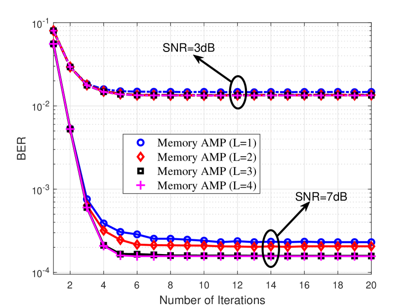
(a) Convergence analysis of Memory AMP with different damping length.
Refer to caption
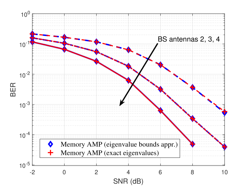
(b) BER performance test of the eigenvalue bounds approximation for different number of BS antennas.
Refer to caption
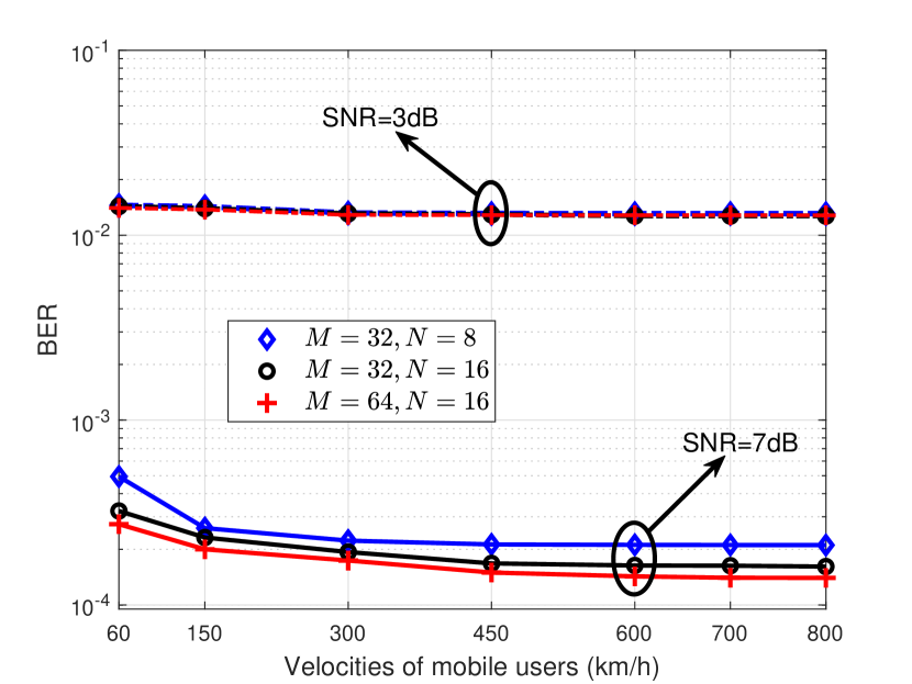
(c) BER performance of Memory AMP for different user velocities and system settings.
Figure 1: Performance test of Memory AMP detector for MIMO-OTFS SCMA systems.

We first investigate the convergence and the effects of damping length on Memory AMP receiver performance. Fig. 1(a) illustrates the bit error rate (BER) performance of Memory AMP versus the number of iterations with different damping length. It can be observed that the BER decreases monotonically and converges within a certain number of iterations. We also notice that no obvious performance improvement after the damping length L>3𝐿3L>3. In the rest of our simulations, we shall use L=3𝐿3L=3 and 𝒯=6𝒯6\mathcal{T}=6 for simplicity.

Fig. 1(b) further tests the effects of the eigenvalue bounds approximation on Memory AMP receiver under different number of BS antennas. It is obvious that the Memory AMP with approximate eigenvalue bounds [13] can achieve similar performance as that of exact eigenvalues. This strongly support the effectiveness of such approximation in Memory AMP. We also note that BER performance improves as the number of BS antennas increases due to the additional spatial diversity.

Fig. 1(c) shows the BER performance of the Memory AMP with different user velocities under various settings of M𝑀M and N𝑁N. As the user velocities increase, the BER performance first improves slightly and then saturates after the velocity beyond 300300300 km/h, particularly for high SNR. This is due to the fact that OTFS modulation can resolve a larger number of distinct paths in Doppler domain for higher velocity, leading to performance benefits. We also observe that the BER performance degrades as M𝑀M and N𝑁N decrease, especially for the higher SNR. This is attributed to the diversity loss caused by the lower resolution of OTFS delay-Doppler grid.

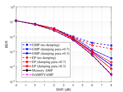
Fig. 2 compares the BER performance of the MIMO-OTFS SCMA systems with different detector algorithms. To highlight the superiority of the proposed Memory AMP algorithm, we also provide the performance of traditional GMP [10, 11], EP [8, 12] and OAMP/VAMP [7] as benchmarks in Fig. 2. The results reveal that the performance of traditional GMP and EP detectors are very sensitive to the damping parameters. Unfortunately, there is no efficient damping solution for GMP and EP detectors currently. However, our developed Memory AMP with closed-form damping solution achieves similar performance to that of OAMP/VAMP even if a low-complexity matched filter is used, and outperforms both the GMP and EP detectors. Based on these analysis, we demonstrate that our Memory AMP detector can yield practical implementation advantage with low complexity and desired performance.
Refer to caption
Figure 2: BER performance comparison for different detector algorithms.

V Conclusion

In this paper, we developed a low-complexity yet effective customized Memory AMP detector, which is suitable for large-scale MIMO-OTFS SCMA system with inherent channel sparsity. In particular, the large-scale matrix inverse is replaced by a finite terms of matrix Taylor series with low-complexity. We applied the specific orthogonality principle and derived an optimal damping solution in Memory AMP detector for better performance. We also analyzed and compared the computational complexity of the Memory AMP with other benchmark detectors. Our results demonstrated that the proposed Memory AMP detector can yield practical implementation advantage with low complexity and desired performance, and outperforms the existing solutions.

Acknowledgment

This study is supported under the RIE2020 Industry Alignment Fund—Industry Collaboration Projects (IAF-ICP) Funding Initiative, as well as cash and in-kind contribution from the industry partner(s).

References

  • [1] R. Hadani et al., “Orthogonal time frequency space modulation,” in Proc. IEEE Wireless Commun. Netw. Conf. (WCNC), San Francisco, CA, USA, Mar. 2017, pp. 1–6.
  • [2] M. Li, S. Zhang, Y. Ge, F. Gao, and P. Fan, “Joint channel estimation and data detection for hybrid RIS aided millimeter wave OTFS systems,” IEEE Trans. Commun., vol. 70, no. 10, pp. 6832–6848, Oct. 2022.
  • [3] Y. Ge, Q. Deng, P. Ching, and Z. Ding, “Receiver design for OTFS with a fractionally spaced sampling approach,” IEEE Trans. Wireless Commun., vol. 20, no. 7, pp. 4072–4086, Jul. 2021.
  • [4] P. Singh, S. Tiwari, and R. Budhiraja, “Low-complexity LMMSE receiver design for practical-pulse-shaped MIMO-OTFS systems,” IEEE Trans. Commun., 2022.
  • [5] H. Qu, G. Liu, M. A. Imran, S. Wen, and L. Zhang, “Efficient channel equalization and symbol detection for MIMO OTFS systems,” IEEE Trans. Wireless Commun., vol. 21, no. 8, pp. 6672–6686, Aug. 2022.
  • [6] T. Thaj and E. Viterbo, “Low-complexity linear diversity-combining detector for MIMO-OTFS,” IEEE Wireless Commun. Lett., vol. 11, no. 2, pp. 288–292, Feb. 2022.
  • [7] Y. Ge, Q. Deng, P. Ching, and Z. Ding, “OTFS signaling for uplink NOMA of heterogeneous mobility users,” IEEE Trans. Commun., vol. 69, no. 5, pp. 3147–3161, May 2021.
  • [8] Y. Ge, Q. Deng, D. González, Y. L. Guan, and Z. Ding, “OTFS signaling for SCMA with coordinated multi-point vehicle communications,” IEEE Trans. Veh. Tech., 2023, doi: 10.1109/TVT.2023.3248119.
  • [9] H. Shao, H. Zhang, H. Zhou, J. Wang, N. Wang, and A. Nallanathan, “A complexity-reduced QRD-SIC detector for interleaved OTFS,” IEEE Trans. Wireless Commun., 2022.
  • [10] P. Raviteja, K. T. Phan, Y. Hong, and E. Viterbo, “Interference cancellation and iterative detection for orthogonal time frequency space modulation,” IEEE Trans. Wireless Commun., vol. 17, no. 10, pp. 6501–6515, Oct. 2018.
  • [11] L. Xiang et al., “Gaussian approximate message passing detection of orthogonal time frequency space modulation,” IEEE Trans. Veh. Tech., vol. 70, no. 10, pp. 10 999–11 004, Oct. 2021.
  • [12] Y. Shan, F. Wang, and Y. Hao, “Orthogonal time frequency space detection via low-complexity expectation propagation,” IEEE Trans. Wireless Commun., 2022.
  • [13] L. Liu, S. Huang, and B. M. Kurkoski, “Memory AMP,” IEEE Trans. Inf. Theory, 2022.
  • [14] K. Xiao et al., “On capacity-based codebook design and advanced decoding for sparse code multiple access systems,” IEEE Trans. Wireless Commun., vol. 17, no. 6, pp. 3834–3849, Jun. 2018.
  • [15] Study on Channel Model for Frequencies From 0.5 to 100 GHz.   Standard 3GPP TR 38.901, 2017.