Translating predictive distributions into informative priors
Abstract
When complex Bayesian models exhibit implausible behaviour, one solution is to assemble available information into an informative prior. Challenges arise as prior information is often only available for the observable quantity, or some model-derived marginal quantity, rather than directly pertaining to the natural parameters in our model. We propose a method for translating available prior information, in the form of an elicited distribution for the observable or model-derived marginal quantity, into an informative joint prior. Our approach proceeds given a parametric class of prior distributions with as yet undetermined hyperparameters, and minimises the difference between the supplied elicited distribution and corresponding prior predictive distribution. We employ a global, multi-stage Bayesian optimisation procedure to locate optimal values for the hyperparameters. Three examples illustrate our approach: a cure-fraction survival model, where censoring implies that the observable quantity is a priori a mixed discrete/continuous quantity; a setting in which prior information pertains to – a model-derived quantity; and a nonlinear regression model.
1 Introduction
A key asset to the Bayesian paradigm is the conceptual ease with which prior information is incorporated into models. For complex, nonlinear, overparameterised, or otherwise partially identified (Gustafson, 2015) models, including such prior information is essential to exclude model behaviours that conflict with reality, and/or known qualities of the phenomena being modelled. Prior information can also improve computation of estimates of the posterior, making otherwise unusable models suitable for inference. However, it is for precisely the models for which prior information is so important that setting appropriate priors for parameters is hardest.
We consider in this paper the task of forming such appropriate informative priors. We distinguish two tasks: predictive elicitation; and the subsequent translation into a prior for a given model. Predictive elicitation is an approach in which elicitation (O’Hagan et al., 2006; Falconer et al., 2021; Low Choy, 2012) proceeds via predictive distributions, often for observable quantities, and is thought to be the most reliable and available form of information (Kadane and Wolfson, 1998). Predictive elicitation is also model-agnostic, meaning the complex, time-consuming process of elicitation does not need to be repeated for each variant of a model. A recent, comprehensive review of elicitation is undertaken by Mikkola et al. (2021).
Translation is the process of using information from predictive elicitation to set the corresponding informative prior for a model. Translation, as a distinct step in the prior specification process, has received less attention than elicitation. A simple predictive approach is to directly model the elicited, observable quantity. This direct approach requires no translation. For example, the Bayesian quantile-parameterised likelihood (Hadlock, 2017; Keelin and Powley, 2011) approach of Perepolkin et al. (2021) involves updating directly elicited information in light of observations. Such direct approaches are currently only feasible for simple models with no latent structure. For models with simple latent structure, it is sometimes possible to elicit information about an invertible function of the parameters (e.g. Chaloner et al., 1993). In these cases it is possible to analytically translate the elicited information into a prior for the parameters. Translation is also clear for conjugate models (Percy, 2002), as if we specify the target prior predictive distribution using the conjugate distribution, then the prior predictive distribution determines the values for the hyperparameters of the prior (related to the idea of “reverse Bayes” in Held et al., 2022). Translation, however, is unclear in general for nonconjugate models (Gribok et al., 2004), although techniques for specific models with specific latent structure are numerous, and include linear regression (Ibrahim, 1997), logistic regression (Bedrick et al., 1997; Chen et al., 1999), Cox models (Chaloner et al., 1993), contingency table analyses (Good, 1967), hierarchical models (Hem, 2021, noting that the space of possible hierarchical models is vast), and autoregressive time-series models (Jarociński and Marcet, 2019). Nevertheless, a model-agnostic approach with a corresponding generic implementation would be preferable, as noted by Gelman et al. (2017) and Mikkola et al. (2021).
Our approach to translation builds on the idea of predictive checks Gabry et al., 2019; Gelman et al., 2017; Box, 1980; Winkler, 1967, the “hypothetical future samples” of; van Zundert et al., 2022, which are an often recommended (Gelman et al., 2020; van Zundert et al., 2022) tool in assessing the concordance of the prior predictive distribution and the elicited predictive information or elicited data distribution. If concordance between these two distributions is low, then the Bayesian workflow (Gelman et al., 2020) proceeds by adjusting the prior to better match the prior predictive distribution to the elicited information. However, for many classes of models, manually adjusting the prior in this manner is infeasible; the complexity required to describe the phenomena of interest muddies the relationship between the prior and the distribution of the observables, and so a more automated method is required. Wang et al. (2018) and Thomas et al. (2020) have proposed approaches in which either regions of observable space or specific realisations are labelled as plausible or implausible by experts, and then an suitable prior formed that accounts for this information, via history matching and a “human in the loop” processes driven by a Gaussian process model respectively. Albert et al. (2012) propose a supra-Bayesian approach intended for multiple experts, in which a Bayesian model is formed for quantiles or probabilities elicited from the experts. Another approach, and the closest in motivation and methodology to ours, is Hartmann et al. 2020; da Silva et al., 2019, which is partly inspired by, which employs a Dirichlet likelihood for elicited predictive quantiles to handle both elicitation and translation.
In this paper we develop a method, and software package, for translation: that is, for constructing an informative prior distribution for model parameters that results in a desired target prior predictive distribution. Using as the starting point for our method a target prior predictive distribution means that our approach is applicable regardless of how the target is elicited, and means that uncertainty is directly and intuitively represented as a distribution. We define a suitable loss function between the prior predictive distribution, given specific values for the hyperparameters of the prior, and this target distribution. The loss function is intentionally generic and permits data that are discrete, continuous, or a mixture thereof. We minimise this loss via a generic, simulation-based, global optimisation process to locate optimal hyperparameters. We highlight throughout that solutions to this optimisation problem are rarely unique, so to regularise the problem we adopt a multiple objective approach. The global optimisation approach is also selected with generality in mind, rendering our method applicable to models where derivative information is unavailable. We make our method available in an R package pbbo333The release used in this paper is available at https://doi.org/10.5281/zenodo.7736707. (R Core Team, 2022). Our method is illustrated in three challenging, moderate dimension problems; a nonlinear regression model, a model using predictive information on a model-derived quantity – a situation not explicitly covered by prior predictive elicitation; and a cure fraction survival model.
2 Translating elicited prior predictive distributions
In this section we propose a set of desirable properties for any translation method, and our mathematical framework and optimisation strategy that together constitute our methodology. We aim to minimise the difference between the prior predictive distribution and our elicited target distribution, whilst also promoting the marginal variance of the model’s parameters. Satisfying the first of these goals produces priors faithful to the supplied information; the second promotes uniqueness and replicability – we elaborate on the precise meaning of these properties momentarily. We adopt a multi-objective optimisation approach to locate priors satisfying these requirements.
2.1 Desiderata
We postulate three key properties that we would like a translation method to satisfy: faithfulness, uniqueness, and replicability.
Faithfulness We consider a prior faithful if it accurately encodes the target data distribution provided by the elicitation subject. Faithfulness is a property of both the model, as it must be possible for the model to represent the information, and the procedure employed to obtain the prior. Especially with simple models and prior structures, not all target prior predictive distributions can be encoded.
Uniqueness In a complex model there may be many prior distributions that imply the same prior predictive distribution. These prior distributions will all be equally faithful. Should uniqueness be desired – and it seems a reasonable enough desiderata most of the time – we must distinguish between priors based on other properties. In Section 2.4 we propose to distinguish priors based on their marginal standard deviations, but other properties could be easily incorporated into our approach.
Replicability We call a procedure/method consistent if it obtains the same, or very similar, prior across independent replications, given the same target. This property is particularly important to assess for methods, like ours, that make use of simulation-based or otherwise stochastic estimates. Global, gradient-free optimisers, when applied to noisy loss functions, offer no guarantee of finding the global minimum in finite time (Liberti, 2008; Mullen, 2014). We assess replicability empirically in all our examples.
These properties are partly inspired by other works in the prior elicitation and specification literature. Faithfulness is closely related to Johnson et al. (2010a)’s definition of validity (see also Johnson et al., 2010b) and O’Hagan et al. (2006)’s use of faithful in Chapter 8 (and throughout the book). However, their concerns are specific to the elicitation process – do the quantities elicited represent what the experts believe? – and not to the subsequent translational step. Our conception of uniqueness and the need for regularisation is noted by da Silva et al. (2019) and Stefan et al. (2022), and is similar to the notion of model sloppiness of Gutenkunst et al. (2007).
We have introduced our desiderata in what we believe to be their order of importance. Firstly, without faithfulness the procedure has not achieved the main aim of translating our knowledge into the prior distribution. Subsequently, given a suite of faithful priors, regularising the problem until it is unique allows us to select one in a clear and replicable way. Such uniqueness inducing regularisation schemes often improve a procedure’s replicability. Replicability ultimately also relies on the empirical behaviour of the procedure when applied to the model of interest. We note that the desiderata are not binary, and at times we may wish to sacrifice some amount of the latter properties for improved faithfulness. We also envisage settings where sacrificing some model flexibility, and thus faithfulness, for a marked increase in replicability increases the usefulness or persuasiveness of a model.
2.2 The target predictive distribution
Our methodology assumes a target predictive distribution (a cumulative distribution function, CDF) for the observable quantity, , has been chosen. The target distribution can be chosen in any manner, but we recommend using predictive elicitation (Kadane and Wolfson, 1998). In brief, such an elicitation proceeds by querying experts about the observable quantity at a small number quantiles, then fitting an appropriate parametric distribution to the elicited values (see Chapter 6 of O’Hagan et al., 2006). We assume a (mixture of) standard distributions can describe the target predictive distribution function , and that we can draw samples from this distribution.
We often wish to elicit information about the observable quantity conditional on some known values of a covariate. For example, when using the linear model we may elicit information about at a fixed set of values for . Further suppose is an experimental design specified before collecting observations of , or comprises observational covariates whose values are known prior to model construction. In such settings we can elicit conditional target distributions .
We elect to describe our methodology in this covariate-specific setting, as it readily reduces to the covariate-independent case.
2.3 Total predictive discrepancy (primary objective)
Consider a joint model for observables and parameters , given hyperparameters and covariates . This joint model has CDF and prior predictive CDF for . Choosing the CDF as the basis for our methodology enables us to be agnostic to whether the observable is continuous, discrete, or a mixture thereof. We will use distribution to refer to the CDF of a stochastic quantity, and density to refer to the corresponding probability density function (where it exists).
Further suppose the target CDF has been elicited at values of the covariate vector denoted , which we stack in the covariate matrix . We assume that each target has identical support to . Lastly, it will be convenient to denote , with and defined analogously.
We quantify the difference between the prior predictive and target by the covariate-specific predictive discrepancy, which we define to be
| (1) |
for some discrepancy function . The Riemann-Stieltjes integral in Equation 1 means this definition applies when is continuous, discrete, or a mixture thereof. Minimising Equation (1) admits the optimal hyperparameter . The covariate-independent equivalent is obtained by setting and ignoring all conditioning on in Equation (1).
The discrepancy function takes two CDFs as its arguments. Inspired by the Cramér-von Mises (von Mises, 1947) and Anderson-Darling (Anderson and Darling, 1952) distributional tests we define, for arbitrary CDFs and , two options for the discrepancy function,
| (2) |
Both discrepancies are proper scoring rules (Gneiting and Raftery, 2007) as they are minimised iff for all . Supposing is flexible enough to exactly match for some , then both discrepancies will yield the same . Differences arise when is insufficiently flexible, in which case Anderson-Darling discrepancy places more emphasis on matching the tails of two CDFs under consideration. Furthermore, we will have to resort to a finite-sample approximation to Equation (1) (which we detail momentarily), and the Anderson-Darling discrepancy is more challenging to accurately compute.
2.4 Regularising estimates of by promoting the marginal standard deviation (secondary objective)
The optimisation problem of minimising Equation (1) is often underspecified. Specifically, there are many optimal values that yield values of that are practically indistinguishable (noted by da Silva et al., 2019) but with immensly differing prior distributions and corresponding marginals for components of . In terms of our desiderata, there are many equally faithful priors (which immediately implies a lack of uniqueness), thus we have an optimisation problem with solutions that are difficult to replicate due to nonuniqueness. This is not surprising because we are providing information only on , which is typically of lower dimension than . A particularly challenging case for uniqueness is in models with additive noise forms (such as Equation (17)). In this case it is challenging to avoid attributing all the variability to the noise term if the prior for the noise is to be specified; in this case it will generally be necessary to fix a prior for the variance using knowledge of the measurement process.
To handle more general cases of lack of uniqueness, we seek to encode the following principle into our methodology: given two estimates of which have equivalent values of , we prefer the one with the larger variance for . This preference induces less of a restriction on the possible values of in the posterior.
We make use of this principle by adopting a multi-objective approach to prior construction and, therefore, now derive a suitable mathematical quantity measuring the variability of . There are numerous suitable functions measuring such variability, and our methodology is agnostic to the particular functional form. Most generally, we define the secondary objective as comprising any such suitable function with
| (3) |
In this paper we consider only one form for , and so hereafter the second objective, which we also seek to minimise, is always
| (4) |
where is the standard deviation of under distribution . This quantity is the mean of the marginal log standard deviations of each of the components of , which we negate so as to promote marginal variability when performing minimisation. We work with the standard deviation (instead of the variance) and take the logarithm thereof to minimise the contribution of any particularly extreme marginal (i.e. marginal with relatively low or high variance). Equations (3) and (4) make explicit the dependence on , and thus , for clarity. We often have analytic expressions for , but precise estimates are also simple to obtain using Monte Carlo. Note that Equation (4) assumes exists, and is nonzero and finite for all and . Should this not be true, for example if one of the marginals of is a Cauchy distribution, we can instead employ alternative, robust estimators of scale (Kravchuk and Pollett, 2012; Rousseeuw and Croux, 1993).
2.5 Post optimisation decision step
We jointly minimise Equations (1) and (4) using a multi-objective optimisation algorithm, which we will cover in Section 2.6. By adopting a multiple objective approach to the translation problem, we obtain a set of possible values which comprise the Pareto frontier , the set of all “non-dominated” choices for , meaning that no point in is preferable in both objectives to any of the remaining points in (for an introduction to multi-objective optimisation problems see Chapter 2 of Deb, 2001). For each in we compute the loss
| (5) |
where the value of expresses our relative belief in the importance of the secondary objective. We take the log of to be on a similar scale to our definition of in Equation (4), but stress that this not necessary should there be a more appropriate scale on which to define . The optimal value is then chosen such that .
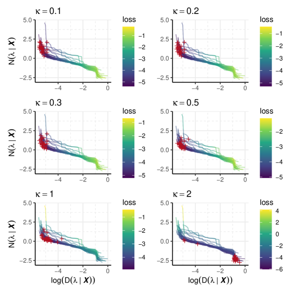
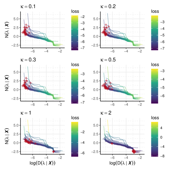
This optimum is clearly sensitive to the choice of . If the relative belief between the two objectives were known, could be set directly, but this will not usually be straightforward to assess. However, the multi-objective optimisation approach makes it computationally inexpensive to test many values of (the set of which we denote with ), and thus plot the Pareto frontier coloured by loss, with the minimum loss point indicated. These can guide our choice of : we can seek a value of with the minimum loss point not on the extreme of the Pareto frontier, since we would like to balance the two objectives. This approach is particularly useful in settings where the scales of the two optima differ markedly, which we further discuss in Appendix C. Where it is feasible to replicate the optimisation procedure, we can additionally seek a choice of that leads to Pareto frontiers with minimal variability across replicates, since this suggests the optimal solution can be estimated reliably.
2.6 Optimisation strategy
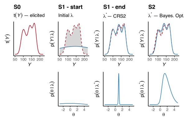
With the mathematical framework defined, we now turn to discuss the many practicalities of optimisation. We use a two-stage global optimisation process to construct a prior with the desiderata listed in Section 2.1. The first stage focuses entirely on faithfulness by minimising only , using the variant of controlled random search 2 (CRS2, Price, 1983) proposed by Kaelo and Ali (2006). Stage one output is then used to initialise stage two, which additionally focuses on uniqueness and replicability by employing multi-objective Bayesian optimisation (Frazier, 2018; Zaefferer et al., 2012) to jointly minimise and . We focus on faithfulness, and thus , as a separate stage because minimising is considerably more challenging than minimising . By initialising stage two with faithful estimates for we can, in the second stage, spend more computational resources on finding points along the Pareto frontier. The resulting optimal prior should suitably encode the information in the target predictive distribution, without being overly confident for model parameters. An idealised form of this process is illustrated in Figure 1.
Note that almost all global optimisation methods require, in the absence of other constraints, to be compact subset of . We require that the practitioner specify the upper/lower limits for each dimension of .
2.6.1 Evaluating the objectives
As noted previously, evaluating for models where analytic results or simple Monte Carlo estimates are available is straightforward, and we denote the corresponding estimate (or, if available, the analytic form) of with . However, there are two immediate challenges to evaluating :
-
1.
the prior predictive CDF is often analytically unavailable;
-
2.
the integral in Equation (1) is almost always intractable.
We address the former with a Monte Carlo based empirical CDF (ECDF), and the latter with importance sampling. Specifically, given a particular value of and , we draw samples with to form the ECDF . To apply importance sampling we rewrite the integral in Equation (1) with respect to importance distribution and Radon-Nikodym derivative , such that
| (6) |
When is discrete or of mixed type, is instead a probability mass function or an appropriate mixture of discrete and continuous densities. Supposing we draw importance samples , we denote the importance sampling approximation to with such that
| (7) |
Note that we write , to make clear that the importance distribution could be covariate-specific, but in straightforward settings a common importance distribution for all covariate values will be appropriate.
We select using information about the support , and samples from and . For more details see Appendix A. Finally, for numerical stability we evaluate on the log scale, with details available in Appendix B. This process is summarised in Algorithm 1.
2.6.2 Optimisation, stage 1
In this stage we focus solely on faithfulness by minimising . We do so using CRS2 (Price, 1983) with local mutation (Kaelo and Ali, 2006), which we run for iterations. We make use of the final optimum value , as well as all of the trial points to obtain a design for the next stage. The design comprises values of , and their corresponding values of . A (small) number of padding points are added to for numerical robustness in stage 2. The result is the design , whose construction is detailed in Algorithm 3 in Appendix D.
Whilst CRS2 was not designed to minimise noisy functions, it appears empirically robust to small quantities of noise. We can make the noise in arbitrarily small (by increasing and ), but doing so usually incurs an enormous computational cost. Carefully balancing the noise in the objective, and thus the quality of the stage one solution, against the cost of evaluation yields a faithful optimum and useful design in an acceptable amount of time.
2.6.3 Optimisation, stage 2
Stage two accounts for the secondary objective in addition to the primary objective. We adjust our optimisation technique to affect this change in emphasis, and use multi-objective Bayesian optimisation, via MSPOT (Zaefferer et al., 2012), to jointly minimise and . MSPOT uses a separate Gaussian process (GP) approximation to each of the objectives, and evaluates these approximations at many points from Latin hypercube designs (Stein, 1987). In each of the iterations, the best points under the current GP approximations are evaluated using the actual objectives. These evaluations accumulate and thus iteratively improve the GP approximations. After iterations, the evaluated points are reduced to their Pareto frontier (Kung et al., 1975). Algorithm 4 in Appendix D describes in detail the MSPOT algorithm as applied to two objectives.
The noisy and computationally expensive nature of our objectives, particularly , necessitates an approach such as MSPOT. Employing approximate GP models for the objectives allows us to screen potential values of inexpensively, and avoid evaluating the actual objectives at values of far from optimal. Moreover, the GP is a flexible yet data efficient model to use as an approximation and can, through appropriate choice of kernel, capture correlation or other complex relationships between components of and the objective.
We use an optional batching technique in stage two because the computational cost of evaluating the GP growing cubically in the number of points used in its construction. Batching avoids this problem by subsampling to remove similar, or otherwise uninformative, points from the collection used to form the surrogate GP model. Specifically, we run MSPOT for a fixed number of iterations, then select a subsample of the points evaluated in the completed batch as initialisation points for the following batch. In our experience this approach can produce equivalent or better priors in less time than a single batch of many iterations. The exact subsampling strategy is detailed in Algorithm 5 in Appendix D.
2.7 Benchmarking and other empirical considerations
We will show results for both the multi-objective approach and the single-objective approach, which does not regularise via the second objective (the optimisation process is identical except stage 2 considers only ).
Having selected we compute the optimal by minimising . Given , we will empirically assess the performance of our method against the desiderata (Section 2.1). Faithfulness is straightforward to assess empirically by comparing the target distribution and the estimated optimal prior predictive distribution . Replicability and uniqueness are more challenging to disentangle empirically: in the absense of replicability, we are not able to conclude whether uniqueness holds or not. We will first assess replicability by examining the stability of the components of the loss in Equation 5 across independent replications of the optimisation procedure. When the loss is stable across replicates, we will assess uniqueness by examining whether the optimal prior predictive distribution and prior are stable across replicates; the stability of both provides good evidence that of uniqueness.
2.8 Summary
Our method for specifying a prior given predictive information requires:
-
1.
a method for sampling ;
-
2.
upper and lower limits that render a compact subset of ;
-
3.
a target CDF which, for numerical stability, must be implemented on the log-scale;
-
4.
a method for generating samples from , as the importance sampler depends on information contained in such samples;
-
5.
a choice of (and we will present a diagnostic plot–see e.g. Figure 10–which assists in making this decision).
Algorithm 2 describes, in pseudocode, our proposed methodology.
2.9 The pbbo R package
We implement our methodology in an R package (R Core Team, 2022) called pbbo, available from https://github.com/hhau/pbbo. pbbo444The release associated with this paper is available at https://doi.org/10.5281/zenodo.6817350. builds on top of mlrMBO (Bischl et al., 2018) for multi-objective Bayesian optimisation, nlopt and nloptr (Ypma et al., 2022; Johnson, 2014) for global optimisation using CRS2 (Kaelo and Ali, 2006), and other packages for internal functionality and logging (Wickham et al., 2019; Rowe, 2016; Maechler et al., 2021). The code implementing the examples we consider in Sections 3 to 5, which further illustrate pbbo, can be found at https://gitlab.com/andrew-manderson/pbbo-paper.
3 Calibrating a cure fraction survival model
Cure models (Peng and Taylor, 2014; Amico and Van Keilegom, 2018) for survival data are useful when a cure mechanism is physically plausible a priori, and when individuals are followed up for long enough to be certain all censored individuals in our data are “cured”. Such lengthy follow ups are not always possible, but a cure model remains plausible when a large fraction of the censored observations occur after the last observed event time. However, we cannot distinguish in the right tail of the survival time distribution between censored uncured individuals and genuinely cured individuals.
We suppose here that we possess prior knowledge on the fraction of individuals likely to be cured, and the distribution of event times amongst the uncured, and seek to translate this information into a reasonable prior for the parameters in a cure model. Consider individuals with event times and censoring times , such that . We suppose censoring times are distributed such that . We simulate data for individuals, each with correlated covariates. We sample a single correlation matrix (Lewandowski et al., 2009) and subsequently covariates . This results in marginally-standardised yet correlated covariates.
There are several properties of this model that make it an interesting subject for prior specification methodology. The observed quantity, and thus the target distribution, is of mixed discrete/continuous type due to censoring. Additionally, we specify a model with a nontrivial correlation structure, about which we wish to specify an informative prior. Eliciting informative priors for correlation structures is known to be challenging. Finally, identifiability is known to be challenging in cure models (Peng and Taylor, 2014), and so the model is a demanding test of our regularisation procedure.
3.1 Target survival time distribution and covariate generation
Suppose that individuals are followed up for an average (but arbitrary) of 21 units of time, with those who experience the event doing so a long time before the end of follow up. Furthermore, suppose we believe that, a priori, of the patients will be cured, with of events censored due to insufficient follow up.
A target distribution that is consistent with our beliefs comprises a point mass of at , and a lognormal distribution with location and scale for . This choice of lognormal has of its mass residing below 21, and thus produces event times that are “well separated” from the censoring time, as required by a cure fraction model. Denoting the lognormal CDF with , we define the target CDF
| (8) |
where is the required normalising constant. This individual-specific construction of implies that the number of covariates , since the censoring time functions as a covariate.
We simulate data for this example with individuals, each with correlated covariates. In line with our target distribution, simulated censoring times are distributed such that . We sample a single correlation matrix (Lewandowski et al., 2009) and subsequently covariates . This results in marginally-standardised yet correlated covariates.
3.2 Model
A cure model for survival data, expressed in terms of its survival function, is
| (9) |
where a proportion of the population are cured and never experience the event of interest. The survival times for the remaining proportion of the population are distributed according to the uncured survival function . We use the tilde in and to denote quantities specific to the uncured survival distribution, and denote to align with our general notation.
Right censoring results in . The censoring indicator is 0 for right censored events, and is 1 otherwise. We denote with the th row of the covariate matrix . Our model supposes that the uncured event times are distributed according to a Weibull regression model, with survival function and hazard such that
| (10) |
with . The likelihood for the th individual is
| (11) | ||||
To align the notation in this example with that introduced in Section 2 we denote and . Note that we are using to represent all information that must be conditioned on, including the censoring times. This is necessary because, in our more general notation, the support of is truncated to an interval that depends on , making the censoring times necessary to fully-specify .
We will seek to identify optimal values of the hyperparamers , where:
| (12) |
The upper and lower limits that define are specified in Table 2 in Appendix E. Our use of the multivariate skew-normal prior has two motivations. The skewness is necessary to incorporate the nonlinear relationship between the hazard and the effect of the covariates, and a covariance structure is used to account for fact that not all the elements of can be large simultaneously. We assume that is marginally (column-wise) standardised, and can thus decompose where is the scale of the prior marginals of . The standardisation allows us to use only one instead of one per covariate. We elect to parameterise using the elements that uniquely determine its Cholesky factor, which we denote . These elements are transformed into using the partial correlation method of Lewandowski et al. (2009), also employed by the Stan math library (Stan Development Team, 2022). The -vector controls, but is not equal to, the marginal skewness for each element of using the multivariate skew-normal definition of Azzalini and Valle (1996), as implemented in the sn package (Azzalini, 2022).
3.3 Tuning parameters and further details
In this example we again employ the multi-objective approach with as defined in Equation 4. We also run single-objective optimisation to facilitate assessing uniqueness. Total predictive discrepancy is computed using both the Anderson-Darling and Cramér-von Mises discrepancy functions.
We use CRS2 iterations, followed by batches of multi-objective Bayesian optimisation using iterations per batch, carrying forward points between batches. The predictive discrepancy function, , is estimated using samples from the prior predictive, and evaluated using importance samples from an appropriate mixed discrete/continuous importance density.
3.4 Results
3.4.1 Choosing for the multi-objective approach
We inspect the Pareto frontiers and compute the minimum loss points for 6 values of . These are displayed, for the Anderson-Darling discrepancy, in Figure 2, and Appendix E.2 Figure 17 for the Cramér-von Mises discrepancy. To reiterate, the assumption is that nearby points on the Pareto frontier are “similar” priors for .
The maximum and minimum values for yield a number of minimum loss points on the extremes of the Pareto frontier. For the maximum, , these points correspond to unsuitable values for due to a lack of faithfulness, which we will demonstrate momentarily. The remaining options for result in similar minimum loss points, illustrating that the minimum loss point is constant, or very similar, across a range of values. Such insensitivity is ideal as we can obtain sensible solutions for a wide variety of values. We select as this simultaneously minimises the variability in loss and both objective functions.
3.4.2 Replicability of loss at the optima
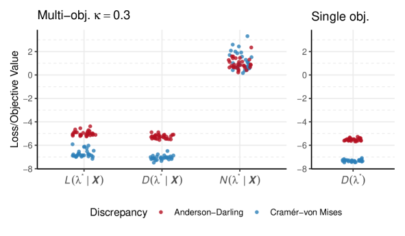
Figure 3 displays , or in the single objective setting, , and at the replicate optima , using in the multi-objective setting. We observe a tight distribution of objective values, particularly for and , suggesting our results are replicable in this example.
3.4.3 Faithfulness
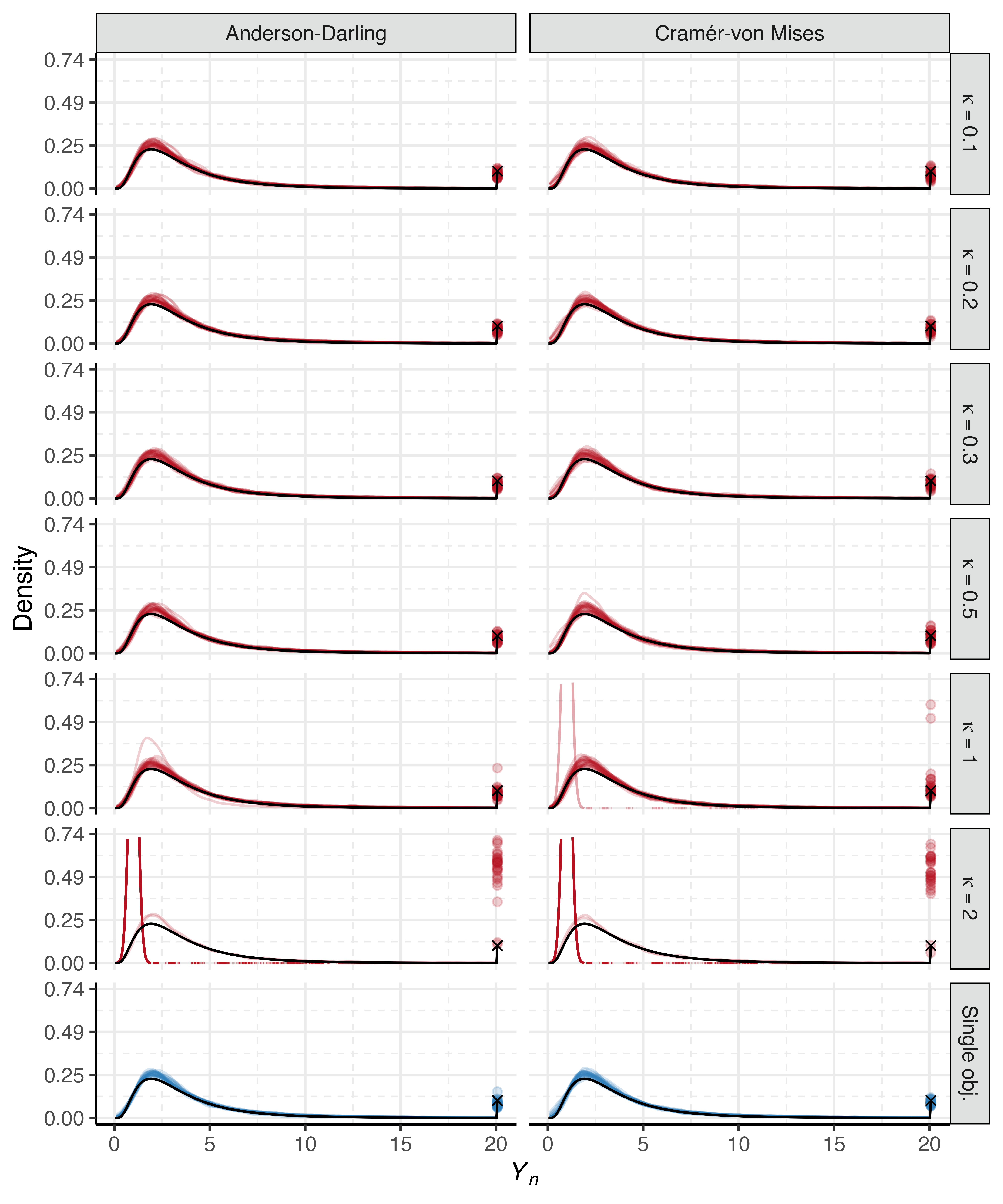
We assess faithfulness by inspecting Figure 4, which displays the prior predictive distributions at the optima and target for the randomly selected individual in our simulated population (other individuals are not visually distinguishable). In addition to the possible values of , the optimal prior predictive distributions are also displayed using the single objective approach for reference. Across all replicates and different , the estimated optimal prior predictive distribution is highly faithful to the target. The multi-objective results are close to those obtained using the single objective approach, except for the two largest values of . By overly valuing the secondary objective, the negative mean log standard deviation, a fraction of the maximum fits are considerably worse. The poor fits correspond to the minimum loss points in the bottom-right corner of the panel in Figure 2.
3.4.4 Uniqueness
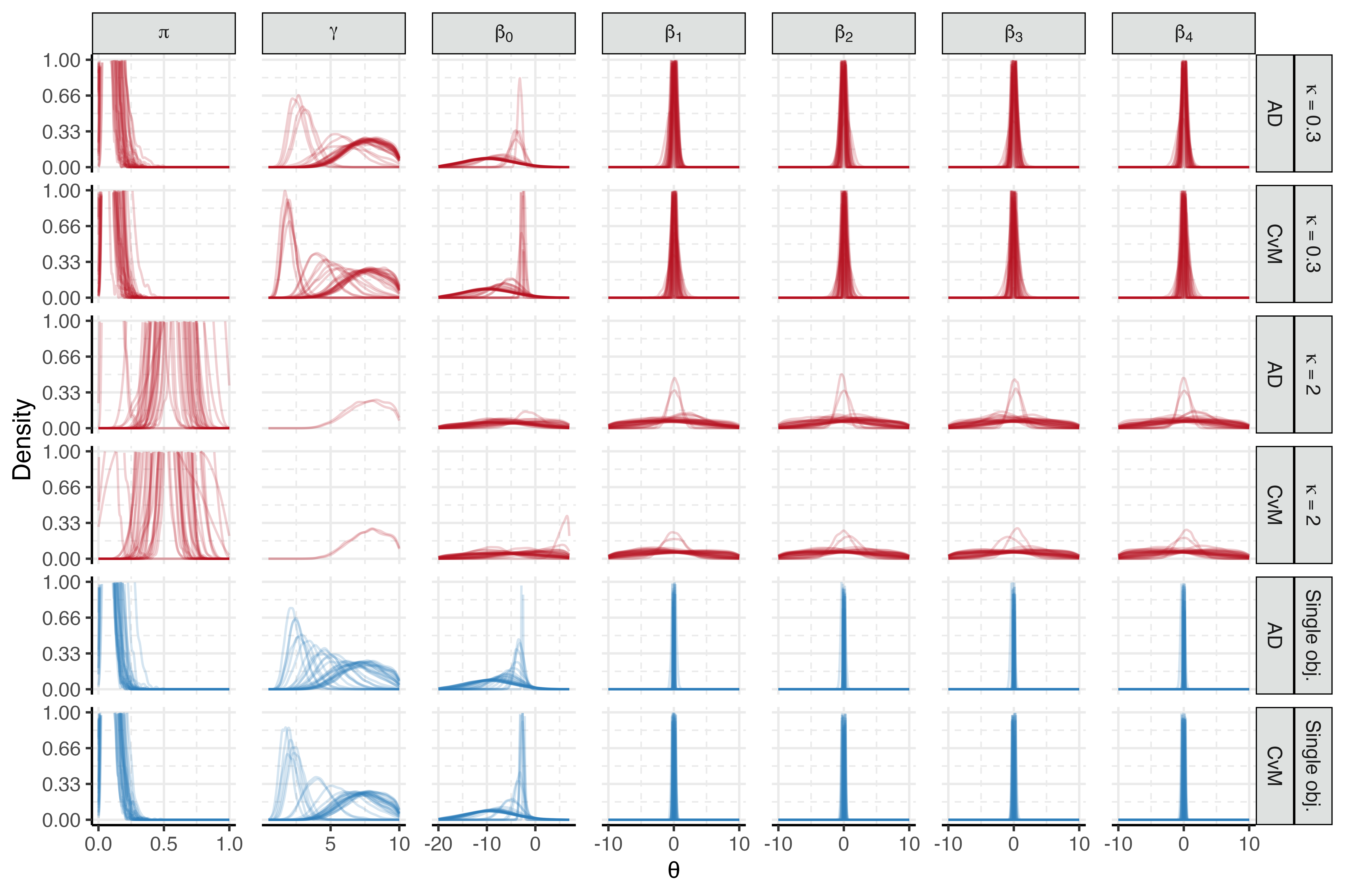
We now evaluate the uniqueness of the optimisation problem. Figure 5 displays the marginals of under both the multi-objective () and the single objective approach, for each independent replicate.
The single objective approach consistently locates the degenerate, non-unique solution where all the variation in the uncensored event times is attributed to the baseline hazard shape and the intercept : i.e. all the mass for (the regression coefficients) is close to 0. The combination of and is evidently poorly identified, and further calculation reveals that only the derived product is uniquely determined. Given the inter-replicate consistency previously observed in Figure 3 we infer that the optimisation process is locating equally good, in terms of predictive discrepancy, optima that correspond to different , which is precisely our definition of nonuniquness. Furthermore, the concentration around means these priors are unlikely to be efficient for inferring the (possible) relationship between covariates and outcome – a very strong signal in the data would be needed to overcome this prior.
Our multi-objective approach produces a more reasonable and disperse prior, but still does not admit a unique optimal prior. The typical marginal prior for has been widened, and for there is a preference for the optima surrounding ; an improvement in uniqueness over the single objective approach, but imperfect. When the process regularly produces a marginal prior for the cure fraction that gives considerable mass to values of , which is incongruent with our target. This is also visible in the censored portions of the prior predictive estimates displayed in Figure 4.
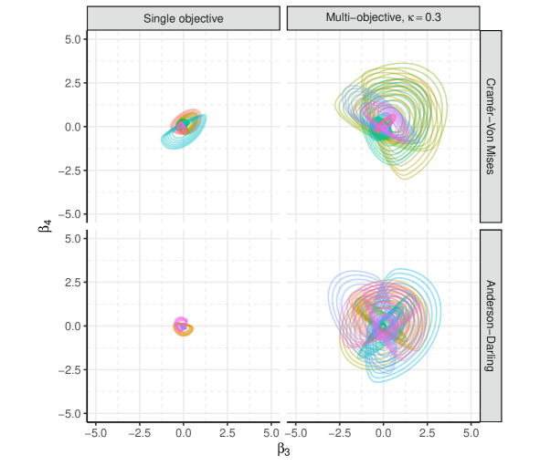
Eliciting covariance structures is challenging, and in this example we included a covariance matrix in the hyperparameters for our model. In Figure 6 we display the bivariate prior marginal densities for two elements of , specifically and , for both the multi-objective approach with and the single objective approach. Nonuniqueness is visible in both sets of estimates. There are marginal densities of both positive and negative marginal skewness, and pairwise correlation. The wider typical marginal for obtained using the multi-objective approach is again visible in the right panel of Figure 6. Lastly, there is a visible difference between the discrepancy functions in the single objective approach, with the Cramer-von Mises discrepancy typically producing a slightly wider marginal.
3.5 Example summary
Our procedure estimates priors that faithfully represent provided information about the survival distribution. Replicability is reasonable in this case, particularly for the loss, although the noise in Figure 2 would, ideally, be smaller. Several priors appear to be consistent with the target distribution we specify, and so the prior our procedure selects is not unique. The multi-objective approach induces more concentration than the single objective approach in the choice of prior for , but it is still not unique. A particular challenge for uniqueness is the covariance structure for the vector of covariate coefficients.
In the information we supply via , we are completely certain of the fraction of cured patients a priori. Such certainty is unlikely to be uncovered when eliciting information from experts. A more elaborate construction of , or elaborate methodology, may be able to represent such uncertainty, but the example remains challenging without this additional complication.
4 Priors from model-derived quantities
Consider the linear model for design matrix and -vector of coefficients indexed by , and where the noise has zero mean and variance . Suppose information about the fraction of variance explained by the model is available – from previous similar experiments, or from knowledge of the measurement process – in the form of a plausible distribution for the coefficient of determination, , which for this model can be computed as
| (13) |
assuming that the columns of have been centred. Our aim is to use our knowledge of to set suitable priors for the regression coefficients . This idea was the inspiration for a class of shrinkage priors (Zhang and Bondell, 2018; Zhang et al., 2022), but we would like to make this idea applicable to a wider selection of prior structures.
To illustrate the effect of including knowledge of on increasingly complicated priors, we investigate the selection of appropriate hyperparameters for three priors for the regression coefficients: two shrinkage priors, and a simple Gaussian prior. We simultaneously vary the covariate-independent target distribution to assess:
-
•
each prior’s ability to faithfully encode the information present across a wide variety of target distributions;
-
•
uniqueness of the optimisation problem, and replicability of the single-objective variant of our optimisation algorithm, for each prior/target pair.
Note that we assume throughout that the noise is distributed according to a Gaussian distribution with zero mean and variance , with an prior on . To demonstrate the challenge that this poses for uniqueness, we will seek to select suitable and using our methodology.
Gaussian prior
The Gaussian prior has only one hyperparameter , which controls the ratio of prior variability due to to that of , and is
| (14) |
Hence, we denote parameters , and seek optimum values for hyperparameters .
Dirichlet-Laplace prior (Dir. Lap.)
Bhattacharya et al. (2015) introduce the Dirichlet-Laplace shrinkage prior, which is defined for the th coefficient such that
| (15) |
There is a single hyperparameter , with smaller values of yielding more sparsity in . Thus we denote and .
Regularised horseshoe prior (Reg. Horse.)
The regularised horseshoe of Piironen and Vehtari (2017) is the most complex of the priors. With more intermediary stochastic quantities between the hyperparameters and , as well as less linearity in the relationship between the aforementioned, it is the most flexible of the priors. These properties make finding optimal values of the hyperparameters more challenging. The prior is
| (16) |
where denotes the Cauchy distribution truncated to . Equation 16 leaves us free to choose three prior-specific hyperparameters, . Thus and . Whilst the regularised horseshoe is carefully designed to make interpretable and easy to choose, here we aim to see if values of these hyperparameters can be chosen to match an informative prior for .
4.1 Target predictive distributions
We consider sixteen different distributions as our target , with and chosen to be four exponentially-spaced values between and including and (i.e. equally-spaced between and ). These values represent a variety of potential forms of the supplied target predictive distribution for .
4.2 Evaluation setup and tuning parameters
We fix and with entries in drawn from a standard Gaussian distribution, and assess replicability using 10 independent runs for each prior and target. The support for the hyperparameters is defined in Table 3 in Appendix F. We run pbbo with samples from the prior predictive distribution, use both and as discrepancy functions, and evaluate the log predictive discrepancy using samples from a importance distribution. We run the first stage of the optimiser for iterations, and subsequently perform both single and multi-objective Bayesian optimisation for batch of iterations, using points from the first stage. The single objective approach illustrates that differences in flexibility between priors also induce differences in uniqueness, and highlights issues in choosing a prior for the additive noise parameter . Choosing is challenging in the multi-objective approach, as its value should depend on the target, the discrepancy function, and the prior. These dependencies result in 96 possible choices of , which is and infeasible number of choices to make in this example. Instead we fix for all multi-objective settings. Lastly, we compute the secondary objective using the marginal standard deviation for all elements in as in Equation (4), except for those quantities where, for some , the standard deviation is undefined. In such cases we use the robust scale estimator from Rousseeuw and Croux (1993).
4.3 Results
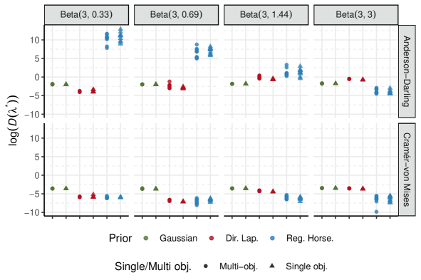
We first assess the replicability of the discrepancy by plotting the value of the objective at the optima across replications. In Figure 7 each value of is the mean of 10 evaluations of at each to minimise residual noise in the objective. Generally, it appears that the discrepancy is replicable for the both Gaussian and Dirichlet-Laplace, for both Anderson-Darling and Cramér-von Mises discrepancies. In contrast, the results for the Regularised Horseshoe prior appear to replicate poorly under the Anderson-Darling discrepancy, but reasonably under the Cramér-von Mises discrepancy.
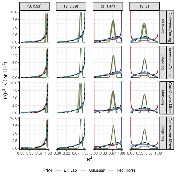
We evaluate the faithfulness of the resulting prior distributions by inspecting the densities and for the various targets (all distributions in this example have corresponding densities). A selected subset of the pairs of values are displayed in Figure 8 (complete results are in Appendix F Figure 21). The faithfulness of the Gaussian prior is universally poor, which we investigate further in Appendix F. Both shrinkage priors perform better in cases where one of or is less than 1, with the regularised horseshoe performing better for the cases. Interestingly, the results are not symmetric in and ; the Dirichlet-Laplace prior is able to match the target well, with many of regularised horseshoe replicates performing poorly; whilst the relative performance is reversed for (see Figure 21). There is also perceptibly more variability in the regularised horseshoe replicates, which suggests the optimisation problem is more challenging and the predictive discrepancy objective is noisier. The multi-objective generally produces more variable sets of optima, which is expected, as it is a more difficult optimisation problem but we do not allow it additional computational resources. There is little visible difference between the two discrepancy functions. Finally, as the values of and increase, the faithfulness of the shrinkage priors generally decreases. Across the full set of simulations, the regularised horseshoe is evidently the most flexible (Appendix F Figure 21).
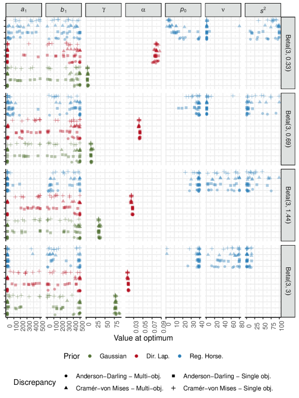
To assess uniqueness, we consider estimated optimal hyperparameter values in each replicate. Figure 9 displays the estimates for and , which corresponds to the targets in Figure 8. The estimates for and , for the Gaussian and Dirichlet-Laplace priors respectively, are consistent across replicates, which suggests the optima may be unique. This remains true even for targets where the prior is not faithful to the target, e.g. the target. There is more variability in the hyperparameters of the regularised horseshoe prior. There does appear to be unique solution for for the and targets, whereas and are highly variable across replicates, which may reflect nonuniqueness or may be due to the lack of replicability (discussed above) of this optimisation for the regularised horseshoe.
The hyperparameters for the additive noise variance are highly variable across replications for almost all prior/target combinations. This reflects the anticipated lack of uniqueness when incorporating such hyperparameters. It is particularly striking for the Dirichlet-Laplace prior when , where we observe consistent and excellent fits/faithfulness to the target, but these do not correspond to replicable estimates for . These settings are also interesting as the choice of single or multi-objective approach greatly impacts the optimum values of and . Faithfulness of the multi-objective optima, illustrated in Figure 8, are not appreciably worse than the single objective approach, but the inclusion of into the secondary objective has resulted in optimal values of and that maximise the dispersion of the marginal prior (i.e. small and large ). Asymptotic results are also known for the Gaussian prior, and in Appendix F we further assess replicability by benchmarking our optimisation process against suitable ‘true’ (asymptotically) values.
4.4 Comparison of discrepancy functions
Our optimisation procedure has minimised using both the Anderson-Darling and Cramér-von Mises discrepancy functions. The former places extra emphasis on matching the tails of the target, and thus the Regularised Horseshoe values in the top row of Figure 7 differ from our expectations given the results in the bottom row of Figure 8. Take, for example, the case. It is plainly evident from Figure 8 that the regularised horseshoe prior provides a better fit to the target distribution at , and yet the corresponding values in the top row of Figure 7 suggest that it is considerably worse that the Gaussian prior at . To reconcile this apparent contradiction, we inspect at the optima computed using the Cramér-Von Mises discrepancy function. These values are displayed in the bottom row of Figure 7, whose values closely match our expectations given Figure 8. Given the range of behaviours of for all the optima, we can conclude that the Anderson-Darling more heavily penalises over-estimation of the tails of than under-estimation. This does not discount it as an optimisation objective, but does complicate comparisons between competing priors.
4.5 Example summary
This example illustrates the use of a model-derived, nonobservable quantity about which we have prior information as the basis for an informative prior. The most flexible shrinkage model (the regularised horseshoe prior) was clearly the most faithful to the supplied information in almost all cases. Conversely, the Gaussian prior is the most replicable and unique, but the lack of faithfulness means it is unsuitable to use as a prior when seeking to use a Beta prior on . The example also illustrates the difficulty of learning about the prior for the additive noise term. Attempts to ameliorate this difficulty by adopting the multi-objective approach merely hide the issue; for the Gaussian and Dirichlet-Laplace priors, where replicability is evident, we always select the inverse gamma prior that maximises the standard deviation of by being on the boundary of . Such a prior for is unlikely to prove appropriate nor represent our prior knowledge.
5 A human-aware prior for a human growth model
We now consider a nonlinear regression model for human growth. There are a number of properties of this example that make it an interesting test for our methodology. First, we find it difficult to specify priors congruent with desired prior predictive distributions for such models; both the nonlinearity and the obvious dependence of height on age complicate prior specification. Data for human growth are also readily available, so we can assess the impact of the prior on many distinct data and posteriors. Second, the model we consider is also poorly behaved under the flat prior, so some prior information is required to stabilise and/or regularise the estimate of the posterior. Finally, this example is also considered by Hartmann et al. (2020), and so there is a suitable comparator for our results.
Suppose an individual has their height measured at age (in years) for , with corresponding measurement (in centimetres). The first Preece-Baines model (Preece and Baines, 1978) for human height is,
| (17) | ||||
| (18) |
with . Some constraints are required to identify this model and ensure its physical plausibility: specifically, we require and . A parameterisation that respects these constraints and is easier to work with uses instead of , and in place of . All of thus have the same positivity constraint. Finally, we also constrain such that . However, these constraints are not sufficient to make the model plausible for all permissible parameter values – the denominator of the fraction can be very small, yielding negative heights.
To align with the notation introduced in Section 2 we denote the parameters by . As in Hartmann et al. (2020), we choose for each of the elements of an independent prior. We will seek to identify the optimal values of . Table 5 in Appendix 5 lists the upper and lower limits we choose for each component of .
We do not consider the measurement error variance as part of . Doing so introduces a degenerate solution for , where all variability in is singularly attributable to and thus . Such a prior seems undesirable, so instead we fix the prior for to reflect the measurement process for human height; measurement errors are unlikely to be more than one or two centimetres, so values of seem reasonable. Thus we set .
5.1 Target predictive distributions
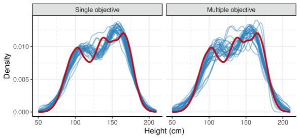
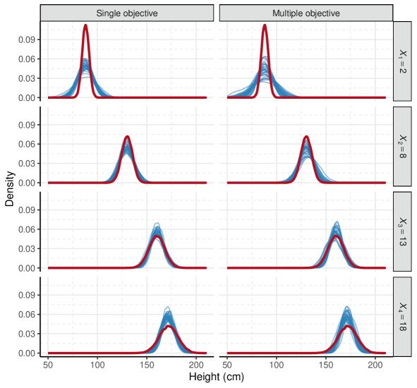
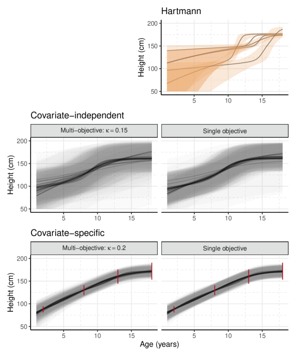
Our data are assumed to originate from a sample of adolescent humans, uniformly distributed between ages 2 and 18, and evenly split between sexes. We consider two different target prior predictive distributions. We first consider a covariate-independent prior predictive density with corresponding CDF for human heights across the entire age-range, derived by summarising external data. This target (Figure 12) is a mixture of 3 gamma densities specified to approximate the external data, which is multimodal due to the fact that humans grow in spurts. We also consider a covariate-specific in which we specify the target predictive distribution of human heights at ages with . Each is normal (see Figure 13, and Appendix G.1 for details).
5.2 Tuning parameters and comparison with Hartmann et. al.
For both targets we obtain using both the single objective and multi-objective optimisation processes (see Sections 2.6 and 2.7). We use only the Cramér-Von Mises discrepancy in this example, because we were not able to reliably compute the Anderson-Darling discrepancy due to numerical instabilities. We run pbbo using samples from and likewise samples from for each of the 4 values of . We use and importance samples, with CRS2 iterations, Bayesian optimisation batches each of iterations, and carry forward points per batch. We assess replicability using 30 independent runs of each objective/target pair.
For this example, we also assess the stability of the posterior: our prior ideally admits a posterior amenable to sampling (i.e. removes spurious modes and eliminates computational difficulties present when using a noninformative prior). It also seems desirable that similar priors should yield similar posteriors. We assess stability by exploit the robust sampling diagnostics in Stan. Should any diagnostic flag an issue with the sampling of the posterior we can be confident that something is amiss with the model, although the converse is not immediately true; a lack of warnings does not imply the model is behaving appropriately.
We compare the priors and posteriors produced by our methodology with the posteriors produced using a flat, improper prior as a benchmark. We consider, separately, each of the 93 individuals in the growth data (Tuddenham and Snyder, 1954) provided by the fda package (Ramsay et al., 2022) in R (R Core Team, 2022). This is a form of prior sensitivity analysis, but distinct from the ideas of Roos et al. (2015) which consider only one particular realisation of the data. By considering each individual in the growth data separately, as opposed to jointly in a hierarchical model, we heighten the importance of including appropriate prior information. We sample each posterior using Stan (Stan Development Team, 2021), setting adapt_delta = 0.95 and max_treedepth = 12 to minimise false positive warning messages.
Hartmann et al. (2020) also considered this example, so we compare also to these results. However, there are key differences between our approaches that must be kept in mind when comparing results. Hartmann et al. (2020) elicit 6 predictive quantiles at ages , as opposed to entire predictive distributions at ages which underpin the covariate-specific version of our method. We use different ages because the model of Preece and Baines (1978) is stated to be accurate and robust for ages greater than 2. Hartmann et al. (2020) include a noise parameter in their definition of . The exact interpretation of this parameter is complicated by their choice of Weibull likelihood, rendering the distribution of the measurement errors sensitive to conditional mean of the model (this is still the case despite their choice of Weibull parameterisation). Finally, Hartmann et al. (2020) elicit quantiles from 5 different users and report an estimated for each user. These estimates (reproduced in Appendix G.3) allow us to compare optimal the selected priors . They do not report whether each user’s estimate is consistent over repeated runs of their optimisation algorithm, and do not discuss the issue of estimate replicability.
5.3 Results
5.3.1 Choosing
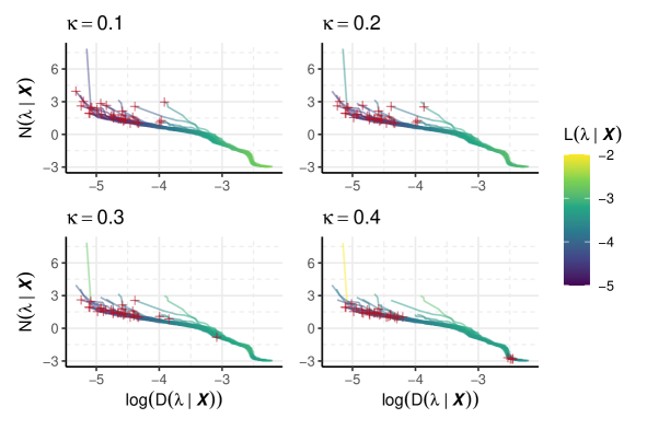
The optimal choice of is target specific, and so we separately choose an appropriate for the covariate-independent and covariate-specific targets. As a heuristic, we choose the value of that yields the minimum variability of for amongst the replicates, though this heuristic is unsuitable if, as we expect to be more commonly the case, only one run of the optimiser is made. In such settings we recommend plotting the Pareto frontiers as in Figure 10 and visually checking that the minimum loss point is not at either extrema of the frontier.
Figure 10 displays Pareto frontiers for a selection of values , and the associated minimum loss points. There is notable inter-replicate variability, with the Pareto frontier for some replicates being totally dominated by other replicates. This is due to the stochastic properties of the global optimisers we employ.
We select for the covariate-specific target given our minimum variability heuristic. Visible in most replicates is an inflection point at values of (the Y-axis in Figure 10) around which the minimum loss points cluster, suggesting any of these points likely admits a reasonable value for . The results for the covariate-independent target are similar (See Appendix G Figure 22) and there we select .
5.3.2 Replicability of discrepancy
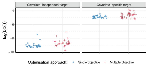
Figure ~11 indicates that, across replicates, the optimisation procedure identifies optimal values with reasonably, but not entirely, consistent predictive discrepancies.
5.3.3 Faithfulness
Figure 12 displays the target and prior predictive density estimates in the covariate-independent case. In the covariate-independent target case, we see that introducing the secondary objective (right panel) produces estimates of that are congruent with estimates from the single objective case, though the estimates are more variable. Both single and multi-objective approaches result in reasonably, but not entirely, faithful densities for . However, most optimum priors seem to accumulates additional probability surrounding , resulting in individual trajectories attaining their adult height for younger than expected ages (which we will later confirm in Figure 14).
For the covariate-specific target, displayed in Figure 13, the secondary objective introduces in some replicates outlying estimates for , most clearly visible for and . Both the single and multi-objective approaches struggle to match the prior predictive distribution at all ages, with consistently poorer faithfulness for . Empirically, it does not seem possible to match all four supplied target prior predictive distributions simultaneously, given the mathematical structure of the model. Lastly, because is substantially narrower than the other targets, it is optimal, under the Cramér-Von Mises discrepancy, to select wider priors better matching the older age target distributions.
5.3.4 Mean prior growth trajectories
We now explore whether the priors we estimate produce reasonable and appropriately uncertain mean growth trajectories a priori. This is similar to our requirement that priors are faithful to the supplied information, but is more general as it considers all possible values of . Figure 14 suggests that both the covariate-independent and covariate-specific targets yield plausible mean growth trajectories. However, the covariate-independent priors are significantly more uncertain, resulting in implausible heights having a priori support. This contrasts with the covariate-specific priors, which interpolate between the supplied targets with an acceptable degree of uncertainty. It is interesting to note that the covariate-specific target has similar levels of uncertainty across all ages, further suggesting that the model may not be flexible enough to simultaneously match all the targets when they have varying variance, as here. All 5 of the priors from Hartmann et al. (2020), for a narrower uncertainty interval, are implausible in both shape and width when viewed on this scale. It also seems unlikely that these priors accurately reflect the information provided by the experts in Hartmann et al. (2020), but this information is not reported.
5.3.5 Posterior stability
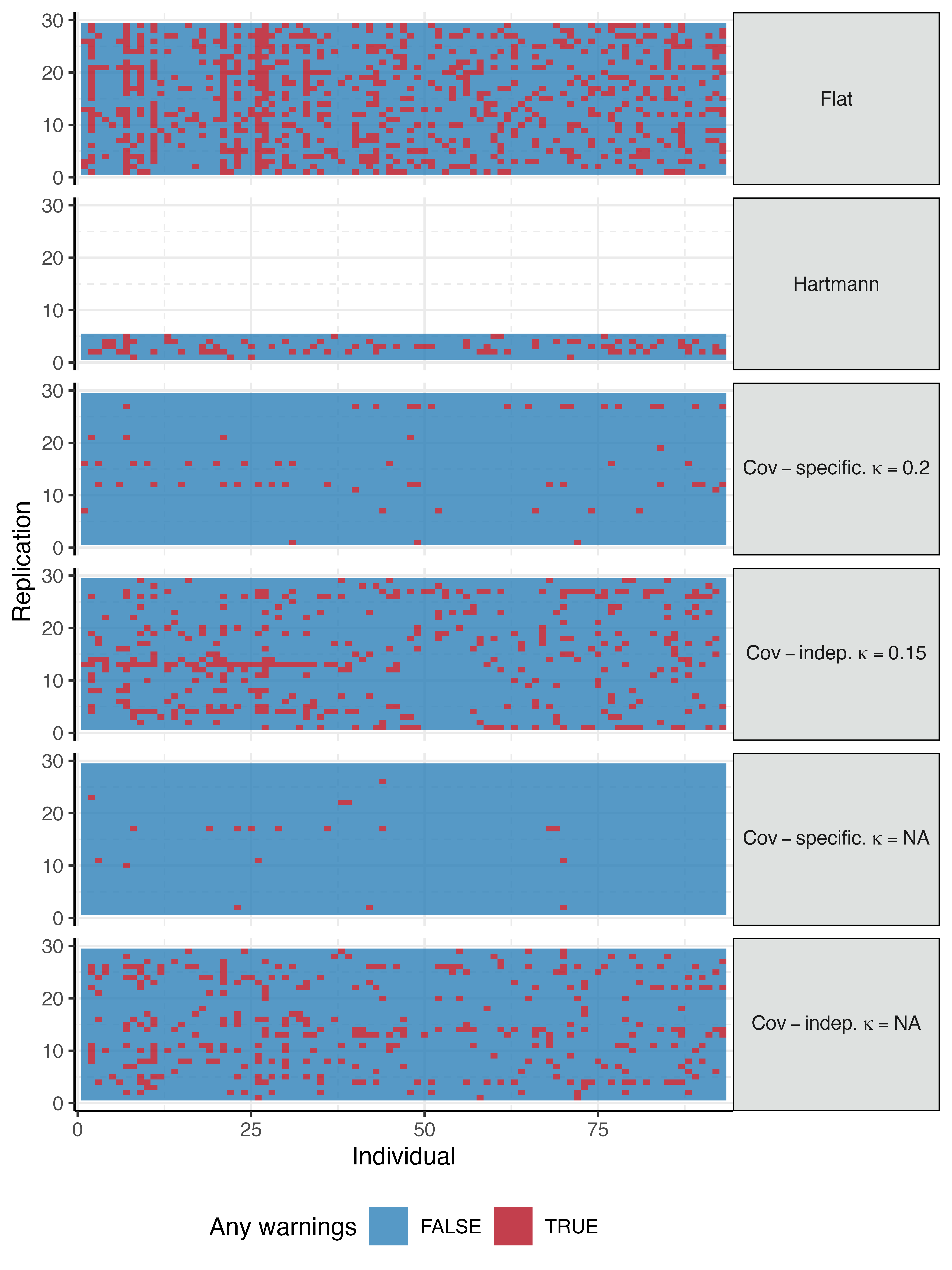
Figure 15 displays for each of the 93 individuals in the growth data whether Stan emits a warning message when estimating the posterior. The flat prior consistently produces posteriors that emit warnings, with some individuals particularly prone to warning messages (i.e. warnings are very correlated within individual columns), suggesting that their data are less informative than other individuals. Warnings are correlated within rows for the Hartmann et. al. priors, indicating that some of the priors are more suitable (replications 1 and 5) for the individuals in the growth data. Amongst our results we note that the covariate-specific approach produces fewer warnings than the covariate-independent approach in both the single- or multi-objective cases. This reflects the additional information available in the covariate-specific setting, and that this information results in more plausible priors. Warnings are particularly correlated within specific priors (i.e. across rows) for the covariate-independent approach, suggesting that these priors are inappropriate for many individuals. The multi-objective approach (third row of Figure 15) produces a small number of additional warnings above the equivalent single-objective approach (fifth row of Figure 15), illustrating the trade-off between single-objective priors that are as informative as possible, and multiple-objective priors that are slightly less informative and thus perform less well in settings where strong prior information is required.
5.3.6 Uniqueness of marginal priors and posteriors
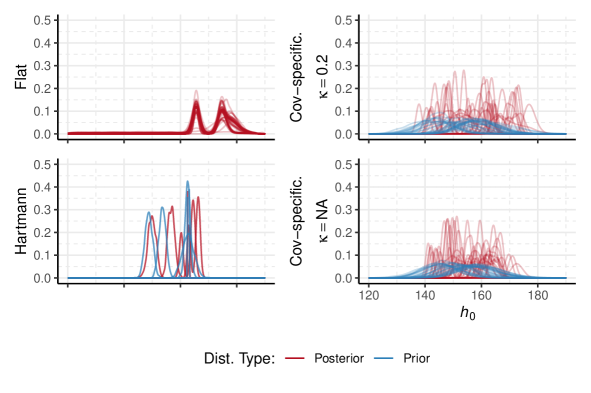
Figure 16 shows the priors for for 30 replicates with the covariate-specific target. The priors for our covariate-specific target exhibit substantial variability. There appear to be two distinct unimodal priors for with similar loss, suggesting that does not provided enough information to uniquely determine a prior distribution. However both priors are significantly broader than the Hartmann et. al. priors. The marginal priors are slightly more consistent for but variability persists.
Figure 16 also shows the posteriors for these parameters when using the (uninformative and thus challenging) data from individual . The flat prior produces a multimodal posterior555We run Stan with the default 4 chains to detect convergence warnings for Figure 15, but in Figure 16 we plot only one chain per replicate to better highlight multi-modal posteriors. for our parameters of interest, demonstrating the lack of stability when computing the posterior and the need for some prior information. As a result, the posteriors are under all methods strongly depend on the prior distribution used, which as noted is not stable under any method here. However, all the possibility of a posterior for with significant mass above 2 is removed by both of our priors, as is desirable, because such solutions correspond to extremely fast growth spurts that are physiologically implausible and are unsupported by the data from individual .
The priors and posteriors for the complete set of parameters are displayed in Appendix G [Figures 23 and 24].
5.4 Example summary
The priors estimated by our procedure in this example are broadly faithful to the supplied information, but appear to be constrained by the model’s inflexibility that makes it difficult to simultaneously match the and targets in the covariate-specific case. They regularise the posterior sufficiently enabling accurate posterior sampling (model inadequacy notwithstanding), with the covariate-specific, multi-objective method proving most useful, but are arguably over concentrated and occasionally prevent the model from fitting the data well. Uniqueness is improved by our secondary objective, but perfect uniqueness across all replicates remains illusive and may not be possible with only the information provided in . We observe a small improvement in uniqueness attributable to the secondary objective (see Appendix G [Figures 23 and 24]); some of the variability may be a result of lack of perfect replicability of the optimisation rather than non-uniqueness.
6 Conclusion
In this paper we develop methodology, and software, for specifying priors given predictive information about an observable or model-derived quantity. We employ a CDF-based, multi-objective global optimisation approach to this translation problem to make our approach widely applicable. Adopting a global optimisation approach allows any kind of model to be specified and optimised, not just those for which we can compute reparameterisation gradients. The global optimisation approach also allows us to provide our functionality directly in R, with which we envisage the majority of the users of our method will be familiar. Our CDF-based predictive discrepancy is also generic as it permits continuous, discrete, and mixed observable types. We apply our methodology in three challenging example models, each of which we interrogate for faithfulness, identifiability, and uniqueness. Each example is of moderate dimension (3–17), with each representing a difficult structural elicitation problem. Finally, our delineation between elicitation and translation, with our emphasis on the latter, is a contribution to an under-explored area of prior specification.
Our inspiration, for both methodology and examples, arises from applications and models we have encountered in applied work. The Preece-Baines model is a typical complex, nonlinear regression model for an intuitive and well understood observable quantity, but for which the model parameters are not easily understood. Setting a prior for models congruent with our knowledge is difficult without a method for translation such as we have proposed. We previously considered a survival model similar to the cure fraction model, where we knew a priori the fraction of cured/censored observations and a distribution of likely survival times, in our earlier work (Manderson and Goudie, 2022). Setting an appropriate prior for this model proved challenging, and would have benefited greatly from the translation methodology introduced in this paper. Finally, prior knowledge on has proved a valuable mathematical basis for the R2-D2 shrinkage prior (Zhang et al., 2022), and more generally there are numerous model-derived quantities about which practitioners possess prior information. Methods for translation are valuable in this setting, as information about such model-derived quantities is often difficult to express. An envisaged future example of this type considers clustering models. In that setting we elicit an informative prior for number of clusters, or the typical size of a cluster, which are derived from the clustering model. Such quantities are readily reasoned about by experts, as opposed to the parameters governing each cluster. Including this type of information in complex models seems critical for stable and reliable Bayesian inference.
One limitation of the current work is that we only partly address non-uniqueness for flexible models and uninformative target distributions. In these settings we emphases that our methodology remains valuable as a means to assess the implications of a particular target distribution on a specific model. For specific model-target pairs where uniqueness remains challenging, our methodology can still provide useful insight into consequences of certain . We can delineate between components of that are well identified and thus consistently estimated, and those that are not. Furthermore, we can directly inspect different significantly from , and consider if such differences are attributable to model inflexibility or implausible targets. Finally, we are compelled to assess our choice of which components should make up , and whether we have other information that we could employ to fix certain components within (e.g. the fixed prior for the noise in the human height example). Another limitation that should be noted is that global optimisation methods lack guarantees of finding the global optimum in finite time, so the the performance of this optimisation process to other problems is unclear.
Acknowledgments and data availability
We thank Daniela De Angelis and Mevin Hooten for their feedback on an earlier version of this manuscript.
This work was supported by The Alan Turing Institute under the UK Engineering and Physical Sciences Research Council (EPSRC) [EP/N510129/1] and the UK Medical Research Council [programme codes MC_UU_00002/2 and MC_UU_00002/20]. No original data were generated as part of this study, the growth data used in Section 5 are available as part of the fda package for R (Ramsay et al., 2022) available on CRAN (https://cran.r-project.org/). For the purpose of open access, the author has applied a Creative Commons Attribution (CC BY) licence to any Author Accepted Manuscript version arising.
Appendices
A Importance sampling
Appropriate importance distributions are crucial to obtaining an accurate and low variance estimate of . For values of far from optimal, can differ considerably from . Given a specific we require an importance distribution that places substantial mass in the high probability regions of both and , as it is in these regions that is largest. But we cannot exert too much effort on finding these densities as they are specific to each value of , and must be found anew for each .
We use three quantities to guide our choice of , these being the support , the samples , and the samples . Of primary concern is the support. If then we use a mixture of Student- distributions; for we employ a mixture of gamma distributions; and for with known , we opt for a mixture of Beta distributions with a discrete component at . The parameters of the mixture components are estimated using the method of moments. Specifically, denoting the empirical mean of as and the empirical variance by , with and defined correspondingly for , Table 1 details our method of moments estimators for the mixture components.
In this paper we limit ourselves to one dimensional , where importance sampling is mostly well behaved or can be tamed using a reasonable amount of computation. This covers many models, and with the covariate-specific target it includes regression models. It is harder to elicit for higher dimensional data spaces, and the difficulties with higher dimensional importance sampling are well known.
| Parameter estimates | Mixture weights | Notes | ||
|---|---|---|---|---|
| defaults to | ||||
|
,
defaults to |
||||
|
,
defaults to |
B Evaluating
For both numerical stability and optimisation performance (Eriksson and Poloczek, 2021; Snoek et al., 2014) we evaluate on the log scale. This is because far from optimal values of have corresponding many orders of magnitude larger than near optimal values of . Furthermore, the Gaussian process approximation that underlies Bayesian optimisation assumes constant variance, necessitating a log or log-like transformation.
Suppose again that we sample , from which we form the ECDF . We also select an appropriate importance distribution and density using Appendix A, and sample importance points . Define the intermediary quantity as
| (19) |
and then rewrite Equation (7) to read
| (20) |
All terms are computed using the numerically stable form (Blanchard et al., 2021).
Accurately evaluating in Equation (19) involves managing the discrete nature of the ECDF (that it returns exactly zero or one for some inputs), and using specialised functions for each discrepancy to avoid issues with floating point arithmetic. We compute using
| (21) |
where . The log-CDF (LCDF) is often more numerically accurate for improbable values of , and so our methodology assumes that it is this LCDF form in which the target distribution is supplied. However, because the ECDF can return exact zero/one values there is no way to perform this computation on the log scale. We thus employ high precision floating point numbers when exponentiating the LCDF values, using Rmpfr (Maechler et al., 2021), to avoid evaluating .
For , additional care must be taken as the denominator of in Equation (2) tends to underflow to zero. Thus we evaluate it using
| (22) |
where is implemented by the Rmpfr package (Maechler, 2012). Such precision is necessary for improbably large values of under T, as the CDF/LCDF often rounds to 1/0 (respectively). It is not always feasible to evaluate Equation (22) with sufficient accuracy to avoid under/over-flow issues – it requires a high-precision implementation of for extreme and many additional bits of precision for both and the result. In these settings we revert to .
C Further notes on choosing
Advantages of multi-objective optimisation are most immediately apparent when the scales of our objectives differ markedly. Consider the equivalent linearised approach, where we select before optimisation and directly optimise . It is generally not possible to know the range of the values of and before optimisation. Selecting an appropriate without this knowledge is prohibitively difficult, leaving only the computationally expensive trial-and-error approach – where we re-run the optimiser for each new possible value of – as a plausible strategy for choosing . In contrast, given it is computationally trivial to recompute for many possible values of after optimisation (e.g. each panel of Figure 10 is trivial to compute). We can thus select in a problem-specific manner for practically no additional computational cost to that of the multi-objective optimiser. Note that the multi-objective optimisation approach is more expensive that the linearised approach, but this additional cost is dwarfed by the number of re-runs of the latter typically required to select .
D Algorithmic descriptions of the optimisation process
D.1 CRS2 as an initialiser for Bayesian optimisation
Algorithm 3 describes our use of CRS2 (Kaelo and Ali, 2006) to obtain a suitable design to initialise the Bayesian multi-objective optimisation approach in step 2.
D.2 MSPOT
Algorithm 4 describes, in our notation, the MSPOT (Zaefferer et al., 2012) algorithm for two objectives. Note that within the algorithm we suppress each objective’s dependence on for brevity.
D.3 Inter batch resampling
Algorithm 5 describes our inter-batch resampling algorithm that we occasionally adopt in stage two of our optimisation process.
E Additional information for the cure fraction survival example
E.1 Hyperparameter support
See Table 2
| Hyperparameter | Lower | Upper | # Elements |
|---|---|---|---|
| 20 | 1 | ||
| 20 | 1 | ||
| -10 | 10 | 1 | |
| 10 | 1 | ||
| 10 | 1 | ||
| -1 + | 1 - | 6 | |
| -5 | 5 | 4 | |
| 1 | 50 | 1 | |
| 1 | 50 | 1 |
E.2 Pareto Frontiers for Cramér-von Mises discrepancy
See Figure 17.
F Additional information for the example
F.1 Hyperparameter support – faithfulness experiment
See Table 3. Note that for the Dirichlet-Laplace prior, Zhang and Bondell (2018) suggest bounding . In our experiments we regularly encountered optimal values of on the lower boundary, so we use instead as a lower bound.
| Prior | Hyperparameter | Lower | Upper |
|---|---|---|---|
| Gaussian | 2 | 500 | |
| Gaussian | 0.2 | 500 | |
| Gaussian | 1 | 500 | |
| Dir. Lap. | 2 | 500 | |
| Dir. Lap. | 0.2 | 500 | |
| Dir. Lap. | |||
| Reg. Horse. | 2 | 500 | |
| Reg. Horse. | 0.2 | 500 | |
| Reg. Horse. | 1 | ||
| Reg. Horse. | 1 | 80 | |
| Reg. Horse. | 100 |
F.2 A comparison to an asymptotic result
The poor fit for the Gaussian prior observed in Figure 8 could be attributed to issues in the optimisation process, or to the lack of flexibility in the prior. To investigate, we compare the results for to Theorem 5 of Zhang and Bondell (2018), which is an asymptotic result regarding the optimal value of for a target density for . We compare pairs of for , noting that assumption (A4) of Zhang and Bondell requires that as (for strictly increasing sequences and ). Thus we consider values of such that with and with and , both for . Each pair is replicated 20 times, and for each replicate we generate a different matrix with standard normal entries. As the target density we choose – a “more Gaussian” target than previously considered and thus, we speculate, possibly more amenable to translation with a Gaussian prior for . We also use this example as an opportunity to assess if there are notable differences between the Cramér-Von Mises discrepancy and the Anderson-Darling discrepancy as defined in Equation (2). The support for differs slightly from the example in the main text, and is defined in Table 4, as matching our target with larger design matrices requires considerably larger values of .
The computation of becomes increasingly expensive as and increase, which limits the value of some of our method’s tuning parameters. The approximate discrepancy function uses samples from the prior predictive and is evaluated using importance samples. We run CRS2 for iterations, using in the initial design for the subsequent single batch of Bayesian optimisation, which uses iterations.
| Prior | Hyperparameter | Lower | Upper |
|---|---|---|---|
| Gaussian | 50 | ||
| Gaussian | 0.2 | 50 | |
| Gaussian | 1 | 5000 |
Results
Figure 18 displays the results in terms of the normalised difference between the we estimate , and the asymptotic result of Zhang and Bondell . Our typical finite sample estimate is slightly larger than the asymptotic result, and the difference increases with and . The variability of the normalised difference remains roughly constant, and thus reduces on an absolute scale, though extrema seem to occur more frequently for larger and . These simulations suggest that the asymptotic regime has not been reached even at the largest and values we assessed.
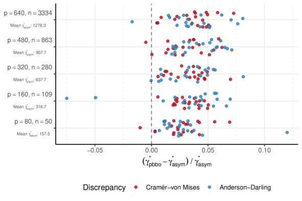
The estimates of are not themselves particularly illuminating: we should instead look for differences in the distribution of at the optima, which is to say on the “data” scale. Figure 19 displays the target distribution and the prior predictive distribution at the optima . The fit is increasingly poor as and increase, and there is little difference both between the two discrepancies and with each discrepancies replications. The lack of difference implies that the optimisation process is consistently locating the same minima for . We conclude that either 1) the ability of the model to match the target depends on there being additional structure in , or 2) it is not possible to encode the information in a prior for into the Gaussian prior.
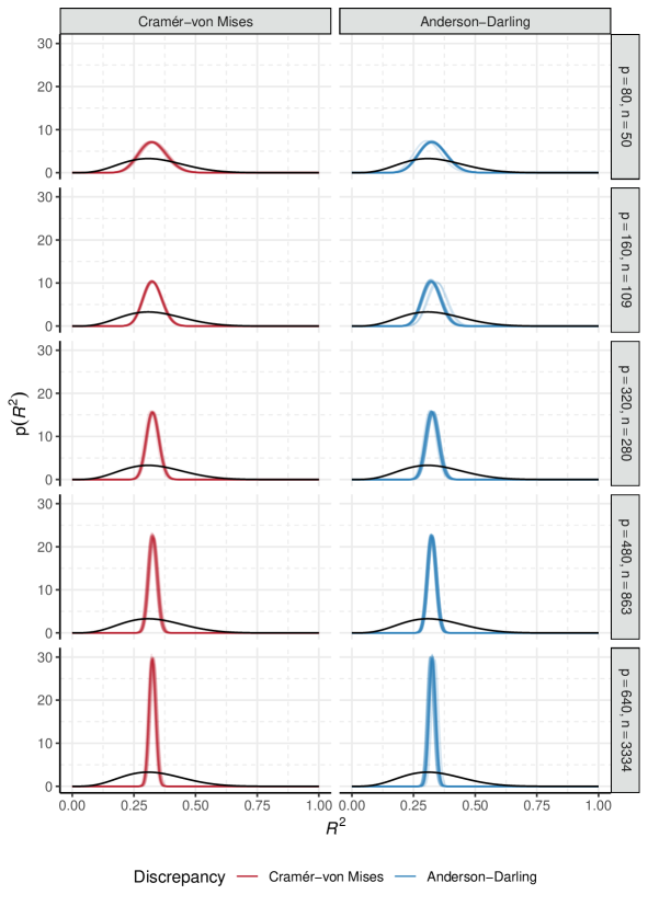
This example also further illustrates the difficulties inherent in acquiring a prior for additive noise terms. Specifically, in this example it is difficult to learn , despite the fact that the contribution of to Equation (13) is not purely additive. However, as we see in Figure 20, estimates are uniformly distributed across the permissible space, except for bunching at the upper and lower bounds of . Note that for numerical and computational stability, we constrain and in this example. This contrasts with similarity between replicates visible in Figure 19, and is thus evidence that have no apparent effect on the value of . We should instead set the prior for based on external knowledge of the measurement process for .
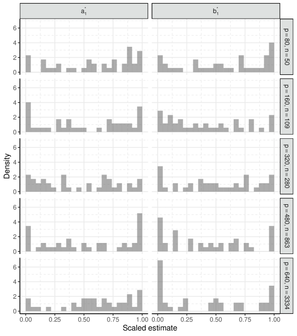
The regularisation method we employ in the two other examples in the main text is unlikely to assist in estimating . Promoting a larger mean log marginal standard deviation, with the knowledge is insensitive to the value of , would simply pick the largest possible value for , which occurs when is at its minimum allowable value and its corresponding maximum.
F.3 Full faithfulness results
The complete results from the faithfulness experiment are displayed in Figure 21.
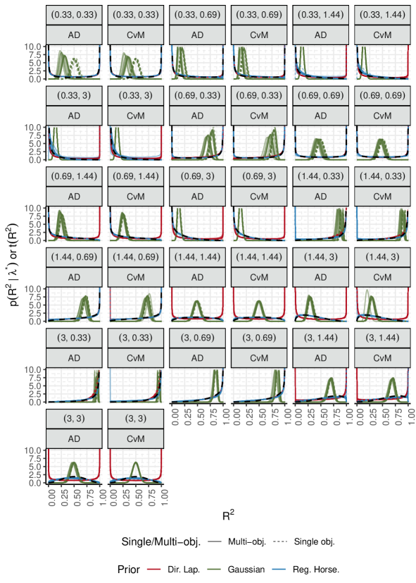
G Additional information for the Preece-Baines example
G.1 Details for and
Denote with the CDF of the gamma distribution with shape parameter and rate ; and the CDF of the normal distribution with mean and standard deviation . We define the covariate-independent target
| (23) |
and the covariate-specific target
| (24) |
G.2 Hyperparameter support
Table 5 contains the upper and lower limits for each hyperparameter, thus defining the feasible region .
| Parameter () | – Lower | – Upper | – Lower | – Upper |
|---|---|---|---|---|
| 130 | 185 | 30 | ||
| 30 | 2 | |||
| 0.2 | 0.1 | |||
| 1.5 | 0.2 | |||
| 9 | 15 | 1 |
G.3 Hartmann et al. (2020) priors
Table 6 contains the priors elicited by Hartmann et al. (2020) (extracted from the supplementary material of that paper) for the parameters in the Preece-Baines example. To generate the prior predictive samples displayed in Figure 14 we draw, for each user, from the corresponding lognormal distribution then compute using Equation (18) (without the error term) and 250 values of spaced evenly between ages and .
| User | Parameter | Expectation | Variance | Lognormal | Lognormal |
|---|---|---|---|---|---|
| 1 | 162.80 | 4.20 | 5.09 | 0.01 | |
| 1 | 174.50 | 0.80 | 5.16 | 0.01 | |
| 1 | 0.10 | 0.10 | -3.50 | 1.55 | |
| 1 | 3.30 | 0.21 | 1.18 | 0.14 | |
| 1 | 13.40 | 0.01 | 2.60 | 0.01 | |
| 2 | 153.73 | 1.60 | 5.04 | 0.01 | |
| 2 | 191.74 | 4.32 | 5.26 | 0.01 | |
| 2 | 0.04 | 0.01 | -4.21 | 1.41 | |
| 2 | 2.00 | 4.30 | 0.33 | 0.85 | |
| 2 | 15.90 | 0.70 | 2.76 | 0.05 | |
| 3 | 148.80 | 1.86 | 5.00 | 0.01 | |
| 3 | 177.14 | 3.68 | 5.18 | 0.01 | |
| 3 | 0.07 | 0.00 | -2.75 | 0.43 | |
| 3 | 4.54 | 37.83 | 0.99 | 1.02 | |
| 3 | 11.31 | 0.21 | 2.42 | 0.04 | |
| 4 | 162.80 | 0.02 | 5.09 | 0.00 | |
| 4 | 174.50 | 0.01 | 5.16 | 0.00 | |
| 4 | 0.10 | 0.01 | -2.65 | 0.83 | |
| 4 | 1.60 | 1.70 | 0.22 | 0.71 | |
| 4 | 14.70 | 0.90 | 2.69 | 0.06 | |
| 5 | 162.60 | 0.85 | 5.09 | 0.01 | |
| 5 | 174.40 | 0.90 | 5.16 | 0.01 | |
| 5 | 0.10 | 0.01 | -2.65 | 0.83 | |
| 5 | 3.40 | 0.01 | 1.22 | 0.03 | |
| 5 | 14.60 | 0.02 | 2.68 | 0.01 |
G.4 Pareto frontiers for the covariate-independent target
The Pareto frontier for the covariate-independent target and all values of is displayed in Figure 22.
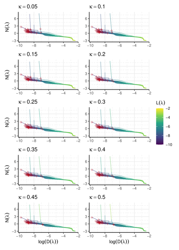
G.5 Full marginal prior and posterior comparison plots
Figures 23 and 24 are extended versions of Figure 16, and display the prior and posterior estimates for all the parameters in . Consistency and uniqueness remain, evidently, challenging and as yet unobtainable.
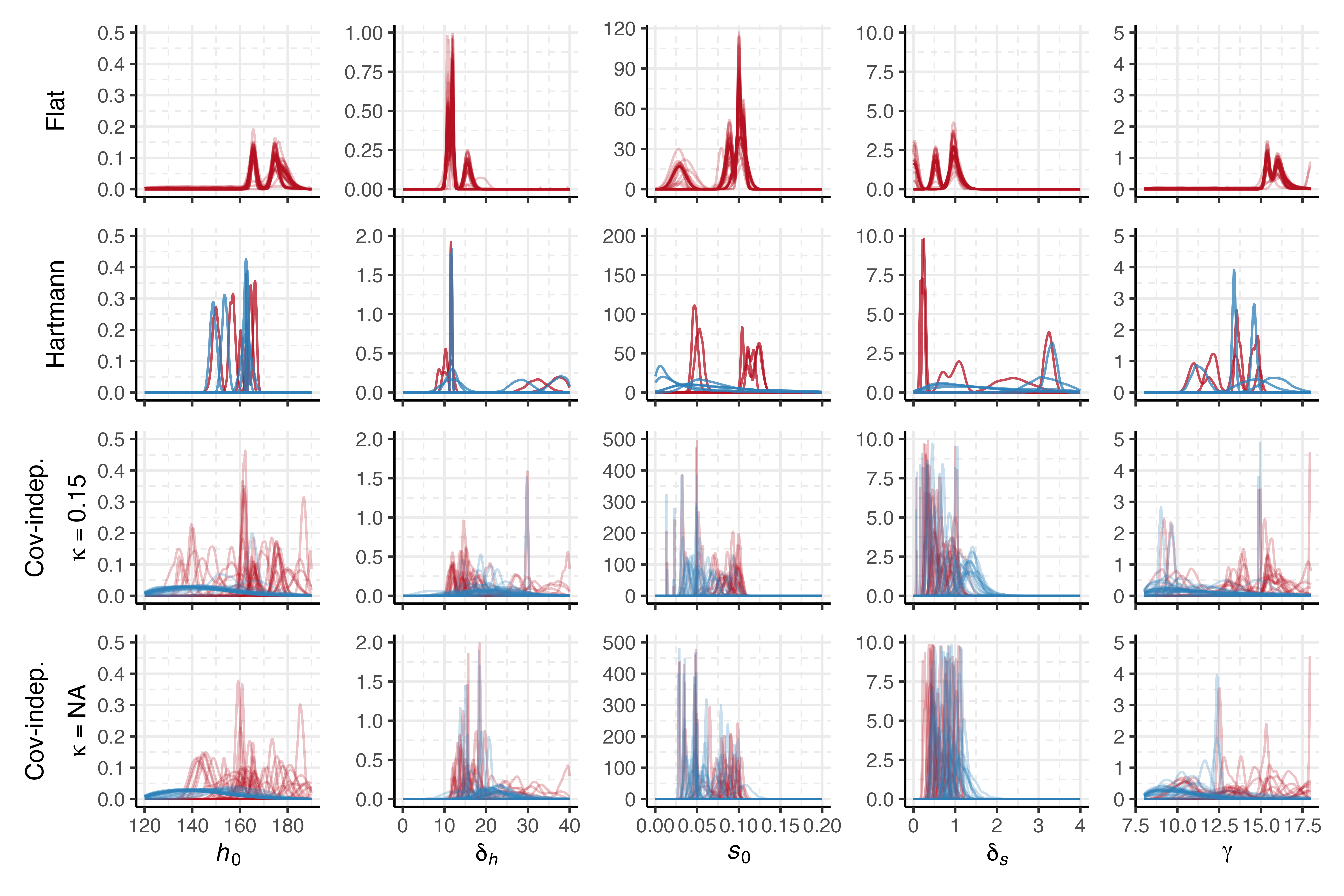
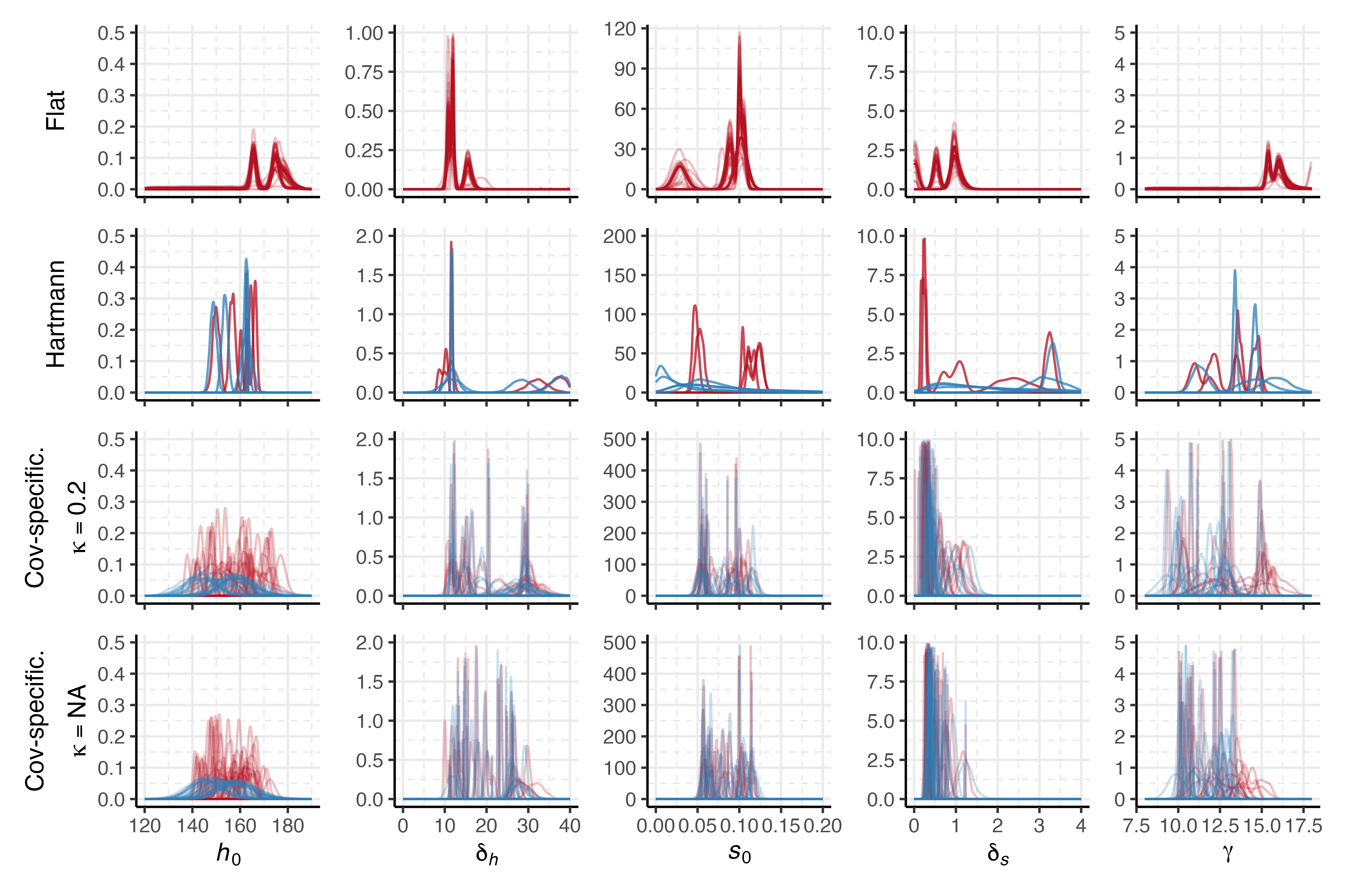
References
- Albert et al. (2012) Albert, I., Donnet, S., Guihenneuc-Jouyaux, C., Low-Choy, S., Mengersen, K., and Rousseau, J. (2012). “Combining expert opinions in prior elicitation,” Bayesian Analysis 7(3), 503–532, doi: 10.1214/12-BA717.
- Amico and Van Keilegom (2018) Amico, M., and Van Keilegom, I. (2018). “Cure Models in Survival Analysis,” Annual Review of Statistics and Its Application 5(1), 311–342, doi: 10.1146/annurev-statistics-031017-100101.
- Anderson and Darling (1952) Anderson, T. W., and Darling, D. A. (1952). “Asymptotic theory of certain "goodness of fit" criteria based on stochastic processes,” The Annals of Mathematical Statistics 23(2), 193–212, doi: 10.1214/aoms/1177729437.
- Azzalini (2022) Azzalini, A. (2022). “sn: The skew-normal and related distributions such as the skew-t and the SUN” .
- Azzalini and Valle (1996) Azzalini, A., and Valle, A. D. (1996). “The multivariate skew-normal distribution,” Biometrika 83(4), 715–726, doi: 10.1093/biomet/83.4.715.
- Bedrick et al. (1997) Bedrick, E. J., Christensen, R., and Johnson, W. (1997). “Bayesian binomial regression: Predicting survival at a trauma center,” The American Statistician 51(3), 211–218, doi: 10.2307/2684890.
- Beume et al. (2009) Beume, N., Fonseca, C. M., Lopez-Ibanez, M., Paquete, L., and Vahrenhold, J. (2009). “On the complexity of computing the hypervolume indicator,” IEEE Transactions on Evolutionary Computation 13(5), 1075–1082, doi: 10.1109/TEVC.2009.2015575.
- Beume et al. (2007) Beume, N., Naujoks, B., and Emmerich, M. (2007). “SMS-EMOA: Multiobjective selection based on dominated hypervolume,” European Journal of Operational Research 181(3), 1653–1669, doi: 10.1016/j.ejor.2006.08.008.
- Bhattacharya et al. (2015) Bhattacharya, A., Pati, D., Pillai, N. S., and Dunson, D. B. (2015). “Dirichlet–laplace priors for optimal shrinkage,” Journal of the American Statistical Association 110(512), 1479–1490, doi: 10.1080/01621459.2014.960967.
- Bischl et al. (2018) Bischl, B., Richter, J., Bossek, J., Horn, D., Thomas, J., and Lang, M. (2018). “mlrMBO: A modular framework for model-based optimization of expensive black-box functions,” arXiv:1703.03373 [stat] .
- Blanchard et al. (2021) Blanchard, P., Higham, D. J., and Nicholas J Higham (2021). “Accurately computing the log-sum-exp and softmax functions,” IMA Journal of Numerical Analysis 41(4), 2311–2330, doi: 10.1093/imanum/draa038.
- Box (1980) Box, G. E. P. (1980). “Sampling and Bayes’ inference in scientific modelling and robustness,” Journal of the Royal Statistical Society: Series A (General) 143(4), 383–404, doi: 10.2307/2982063.
- Chaloner et al. (1993) Chaloner, K., Church, T., Louis, T. A., and Matts, J. P. (1993). “Graphical elicitation of a prior distribution for a clinical trial,” Journal of the Royal Statistical Society. Series D (The Statistician) 42(4), 341–353, doi: 10.2307/2348469.
- Chen et al. (1999) Chen, M.-H., Ibrahim, J. G., and Yiannoutsos, C. (1999). “Prior elicitation, variable selection and Bayesian computation for logistic regression models,” Journal of the Royal Statistical Society. Series B (Statistical Methodology) 61(1), 223–242.
- da Silva et al. (2019) da Silva, E. d. S., Kuśmierczyk, T., Hartmann, M., and Klami, A. (2019). “Prior specification via prior predictive matching: Poisson matrix factorization and beyond,” arXiv:1910.12263 [cs, stat] .
- Deb (2001) Deb, K. (2001). Multi-Objective Optimization Using Evolutionary Algorithms, 1st ed ed. (John Wiley & Sons, Chichester; New York).
- Deb et al. (2002) Deb, K., Pratap, A., Agarwal, S., and Meyarivan, T. (2002). “A fast and elitist multiobjective genetic algorithm: NSGA-II,” IEEE Transactions on Evolutionary Computation 6(2), 182–197, doi: 10.1109/4235.996017.
- Eriksson and Poloczek (2021) Eriksson, D., and Poloczek, M. (2021). “Scalable constrained Bayesian optimization,” in Proceedings of The 24th International Conference on Artificial Intelligence and Statistics, PMLR, pp. 730–738.
- Falconer et al. (2021) Falconer, J. R., Frank, E., Polaschek, D. L. L., and Joshi, C. (2021). “Methods for eliciting informative prior distributions,” arXiv:2112.07090 [stat] .
- Frazier (2018) Frazier, P. I. (2018). “A tutorial on Bayesian optimization,” arXiv:1807.02811 [cs, math, stat] .
- Gabry et al. (2019) Gabry, J., Simpson, D., Vehtari, A., Betancourt, M., and Gelman, A. (2019). “Visualization in Bayesian workflow,” Journal of the Royal Statistical Society: Series A (Statistics in Society) 182(2), 389–402, doi: 10.1111/rssa.12378.
- Gelman et al. (2017) Gelman, A., Simpson, D., and Betancourt, M. (2017). “The prior can often only be understood in the context of the likelihood,” Entropy 19(10), 555, doi: 10.3390/e19100555.
- Gelman et al. (2020) Gelman, A., Vehtari, A., Simpson, D., Margossian, C. C., Carpenter, B., Yao, Y., Kennedy, L., Gabry, J., Bürkner, P.-C., and Modrák, M. (2020). “Bayesian workflow,” arXiv:2011.01808 [stat] .
- Gneiting and Raftery (2007) Gneiting, T., and Raftery, A. E. (2007). “Strictly proper scoring rules, prediction, and estimation,” Journal of the American Statistical Association 102(477), 359–378, doi: 10.1198/016214506000001437.
- Good (1967) Good, I. J. (1967). “A Bayesian significance test for multinomial distributions,” Journal of the Royal Statistical Society: Series B (Methodological) 29(3), 399–418, doi: 10.1111/j.2517-6161.1967.tb00705.x.
- Gribok et al. (2004) Gribok, A. V., Urmanov, A. M., Wesley Hines, J., and Uhrig, R. E. (2004). “Backward specification of prior in Bayesian inference as an inverse problem,” Inverse Problems in Science and Engineering 12(3), 263–278, doi: 10.1080/10682760310001598689.
- Gustafson (2015) Gustafson, P. (2015). Bayesian Inference for Partially Identified Models: Exploring the Limits of Limited Data (CRC Press, Taylor & Francis Group).
- Gutenkunst et al. (2007) Gutenkunst, R. N., Waterfall, J. J., Casey, F. P., Brown, K. S., Myers, C. R., and Sethna, J. P. (2007). “Universally sloppy parameter sensitivities in systems biology models,” PLoS computational biology 3(10), 1871–1878, doi: 10.1371/journal.pcbi.0030189.
- Hadlock (2017) Hadlock, C. C. (2017). “Quantile-parameterized methods for quantifying uncertainty in decision analysis,” Thesis, doi: 10.15781/T2F18SX41.
- Hartmann et al. (2020) Hartmann, M., Agiashvili, G., Bürkner, P., and Klami, A. (2020). “Flexible prior elicitation via the prior predictive distribution,” in Proceedings of the 36th Conference on Uncertainty in Artificial Intelligence (UAI), PMLR, pp. 1129–1138.
- Held et al. (2022) Held, L., Matthews, R., Ott, M., and Pawel, S. (2022). “Reverse-Bayes methods for evidence assessment and research synthesis,” Research Synthesis Methods 13(3), 295–314, doi: 10.1002/jrsm.1538.
- Hem (2021) Hem, I. G. (2021). “Robustifying Bayesian hierarchical models using intuitive prior elicitation,” Ph.D. thesis, Norwegian University of Science and Technology.
- Ibrahim (1997) Ibrahim, J. G. (1997). “On properties of predictive priors in linear models,” The American Statistician 51(4), 333–337, doi: 10.1080/00031305.1997.10474408.
- Jarociński and Marcet (2019) Jarociński, M., and Marcet, A. (2019). “Priors about observables in vector autoregressions,” Journal of Econometrics 209(2), 238–255, doi: 10.1016/j.jeconom.2018.12.023.
- Johnson (2014) Johnson, S. G. (2014). “The NLopt nonlinear-optimization package” .
- Johnson et al. (2010a) Johnson, S. R., Tomlinson, G. A., Hawker, G. A., Granton, J. T., and Feldman, B. M. (2010a). “Methods to elicit beliefs for Bayesian priors: A systematic review,” Journal of Clinical Epidemiology 63(4), 355–369, doi: 10.1016/j.jclinepi.2009.06.003.
- Johnson et al. (2010b) Johnson, S. R., Tomlinson, G. A., Hawker, G. A., Granton, J. T., Grosbein, H. A., and Feldman, B. M. (2010b). “A valid and reliable belief elicitation method for Bayesian priors,” Journal of Clinical Epidemiology 63(4), 370–383, doi: 10.1016/j.jclinepi.2009.08.005.
- Kadane and Wolfson (1998) Kadane, J., and Wolfson, L. J. (1998). “Experiences in elicitation,” Journal of the Royal Statistical Society: Series D (The Statistician) 47(1), 3–19, doi: 10.1111/1467-9884.00113.
- Kaelo and Ali (2006) Kaelo, P., and Ali, M. M. (2006). “Some variants of the controlled random search algorithm for global optimization,” Journal of Optimization Theory and Applications 130(2), 253–264, doi: 10.1007/s10957-006-9101-0.
- Keelin and Powley (2011) Keelin, T. W., and Powley, B. W. (2011). “Quantile-parameterized distributions,” Decision Analysis 8(3), 206–219, doi: 10.1287/deca.1110.0213.
- Kravchuk and Pollett (2012) Kravchuk, O. Y., and Pollett, P. K. (2012). “Hodges-Lehmann scale estimator for Cauchy distribution,” Communications in Statistics - Theory and Methods 41(20), 3621–3632, doi: 10.1080/03610926.2011.563016.
- Kung et al. (1975) Kung, H. T., Luccio, F., and Preparata, F. P. (1975). “On finding the maxima of a set of vectors,” Journal of the ACM 22(4), 469–476, doi: 10.1145/321906.321910.
- Lewandowski et al. (2009) Lewandowski, D., Kurowicka, D., and Joe, H. (2009). “Generating random correlation matrices based on vines and extended onion method,” Journal of Multivariate Analysis 100(9), 1989–2001, doi: 10.1016/j.jmva.2009.04.008.
- Liberti (2008) Liberti, L. (2008). “Introduction to global optimization,” 43.
- Low Choy (2012) Low Choy, S. (2012). “Priors: Silent or active partners of Bayesian inference?,” in Case Studies in Bayesian Statistical Modelling and Analysis, edited by C. L. Alston, K. L. Mengersen, and A. N. Pettitt (John Wiley & Sons, Ltd), Chap. 3, pp. 30–65, doi: 10.1002/9781118394472.ch3.
- Maechler (2012) Maechler, M. (2012). “Accurately computing log(1 - exp(-|a|)) assessed by the Rmpfr package,” 9.
- Maechler et al. (2021) Maechler, M., Heiberger, R. M., Nash, J. C., and Borchers, H. W. (2021). “Rmpfr: R MPFR - multiple precision floating-point reliable” .
- Manderson and Goudie (2022) Manderson, A. A., and Goudie, R. J. B. (2022). “Combining chains of Bayesian models with Markov melding,” Bayesian Analysis -1(-1), 1–34, doi: 10.1214/22-BA1327.
- Mikkola et al. (2021) Mikkola, P., Martin, O. A., Chandramouli, S., Hartmann, M., Pla, O. A., Thomas, O., Pesonen, H., Corander, J., Vehtari, A., Kaski, S., Bürkner, P.-C., and Klami, A. (2021). “Prior knowledge elicitation: The past, present, and future,” arXiv:2112.01380 [stat] .
- Mullen (2014) Mullen, K. M. (2014). “Continuous global optimization in R,” Journal of Statistical Software 60, 1–45, doi: 10.18637/jss.v060.i06.
- O’Hagan et al. (2006) O’Hagan, A., Buck, C., Daneshkhah, A., Eiser, J., Garthwaite, P., Jenkinson, D., Oakley, J., and Rakow, T. (2006). Uncertain Judgements: Eliciting Experts’ Probabilities (Wiley).
- Peng and Taylor (2014) Peng, Y., and Taylor, J. M. G. (2014). “Cure Models,” in Handbook of Survival Analysis, edited by J. P. Klein, H. C. van Houwelingen, J. G. Ibrahim, and T. H. Scheike, Handbooks of Modern Statistical Methods (Routledge Handbooks Online), doi: 10.1201/b16248-8.
- Percy (2002) Percy, D. F. (2002). “Bayesian enhanced strategic decision making for reliability,” European Journal of Operational Research 139(1), 133–145, doi: 10.1016/S0377-2217(01)00177-1.
- Perepolkin et al. (2021) Perepolkin, D., Goodrich, B., and Sahlin, U. (2021). “Hybrid elicitation and indirect Bayesian inference with quantile-parametrized likelihood” doi: 10.31219/osf.io/paby6.
- Piironen and Vehtari (2017) Piironen, J., and Vehtari, A. (2017). “Sparsity information and regularization in the horseshoe and other shrinkage priors,” Electronic Journal of Statistics 11(2), 5018–5051, doi: 10.1214/17-EJS1337SI.
- Preece and Baines (1978) Preece, M., and Baines, M. (1978). “A new family of mathematical models describing the human growth curve,” Annals of Human Biology 5(1), 1–24, doi: 10.1080/03014467800002601.
- Price (1983) Price, W. L. (1983). “Global optimization by controlled random search,” Journal of Optimization Theory and Applications 40(3), 333–348, doi: 10.1007/BF00933504.
- R Core Team (2022) R Core Team (2022). “r: A language and environment for statistical computing” R Foundation for Statistical Computing.
- Ramsay et al. (2022) Ramsay, J. O., Graves, S., and Hooker, G. (2022). “fda: Functional data analysis” .
- Roos et al. (2015) Roos, M., Martins, T. G., Held, L., and Rue, H. (2015). “Sensitivity analysis for Bayesian hierarchical models,” Bayesian Analysis 10(2), 321–349, doi: 10.1214/14-BA909.
- Rousseeuw and Croux (1993) Rousseeuw, P. J., and Croux, C. (1993). “Alternatives to the median absolute deviation,” Journal of the American Statistical Association 88(424), 1273–1283, doi: 10.2307/2291267.
- Rowe (2016) Rowe, B. L. Y. (2016). “futile.logger: A Logging Utility for R” .
- Snoek et al. (2014) Snoek, J., Swersky, K., Zemel, R., and Adams, R. (2014). “Input warping for Bayesian optimization of non-stationary functions,” in Proceedings of the 31st International Conference on Machine Learning, PMLR, pp. 1674–1682.
- Stan Development Team (2021) Stan Development Team (2021). “rstan: The R interface to Stan” .
- Stan Development Team (2022) Stan Development Team (2022). “Stan modeling language: User’s guide and reference manual” .
- Stefan et al. (2022) Stefan, A. M., Evans, N. J., and Wagenmakers, E.-J. (2022). “Practical challenges and methodological flexibility in prior elicitation,” Psychological Methods 27(2), 177–197, doi: 10.1037/met0000354.
- Stein (1987) Stein, M. (1987). “Large sample properties of simulations using Latin hypercube sampling,” Technometrics 29(2), 143–151, doi: 10.2307/1269769.
- Thomas et al. (2020) Thomas, O., Pesonen, H., and Corander, J. (2020). “Probabilistic elicitation of expert knowledge through assessment of computer simulations,” arXiv:2002.10902 [stat] .
- Tuddenham and Snyder (1954) Tuddenham, R. D., and Snyder, M. M. (1954). “Physical growth of California boys and girls from birth to eighteen years,” Publications in Child Development. University of California, Berkeley 1(2), 183–364.
- van Zundert et al. (2022) van Zundert, C., Somer, E., and Miočević, M. (2022). “Prior predictive checks for the method of covariances in Bayesian mediation analysis,” Structural Equation Modeling: A Multidisciplinary Journal 29(3), 428–437, doi: 10.1080/10705511.2021.1977648.
- von Mises (1947) von Mises, R. (1947). “On the asymptotic distribution of differentiable statistical functions,” The Annals of Mathematical Statistics 18(3), 309–348, doi: 10.1214/aoms/1177730385.
- Wang et al. (2018) Wang, X., Nott, D. J., Drovandi, C. C., Mengersen, K., and Evans, M. (2018). “Using history matching for prior choice,” Technometrics 60(4), 445–460, doi: 10.1080/00401706.2017.1421587.
- Wickham et al. (2019) Wickham, H., Averick, M., Bryan, J., Chang, W., McGowan, L., François, R., Grolemund, G., Hayes, A., Henry, L., Hester, J., Kuhn, M., Pedersen, T., Miller, E., Bache, S., Müller, K., Ooms, J., Robinson, D., Seidel, D., Spinu, V., Takahashi, K., Vaughan, D., Wilke, C., Woo, K., and Yutani, H. (2019). “Welcome to the Tidyverse,” Journal of Open Source Software 4(43), 1686, doi: 10.21105/joss.01686.
- Winkler (1967) Winkler, R. L. (1967). “The assessment of prior distributions in Bayesian analysis,” Journal of the American Statistical Association 62(319), 776–800, doi: 10.1080/01621459.1967.10500894.
- Ypma et al. (2022) Ypma, J., Johnson, S. G., Borchers, H. W., Eddelbuettel, D., Ripley, B., Hornik, K., Chiquet, J., Adler, A., Dai, X., Stamm, A., and Ooms, J. (2022). “nloptr: R interface to NLopt” .
- Zaefferer et al. (2012) Zaefferer, M., Bartz-Beielstein, T., Friese, M., Naujoks, B., and Flasch, O. (2012). “mspot: Multi-criteria sequential parameter optimization” .
- Zhang and Bondell (2018) Zhang, Y., and Bondell, H. D. (2018). “Variable selection via penalized credible regions with Dirichlet–Laplace global-local shrinkage priors,” Bayesian Analysis 13(3), doi: 10.1214/17-BA1076.
- Zhang et al. (2022) Zhang, Y. D., Naughton, B. P., Bondell, H. D., and Reich, B. J. (2022). “Bayesian regression using a prior on the model fit: The R2-D2 shrinkage prior,” Journal of the American Statistical Association 117(538), 862–874, doi: 10.1080/01621459.2020.1825449.