Errata to Stochastic explosion and non-uniqueness for -Riccati equation
Abstract
An error occurs in a part of the statement and proof of Proposition 2.2 in the paper “Stochastic explosion and non-uniqueness for -Riccati equation”, Jour. Math. Anal. and Appl., 476, (2019), 53-85 that is corrected in this errata. The revised result reveals a new and unexpected critical phenomena, having further implications for non-uniqueness of solutions to a nonlinear differential equation of the Riccati type.
1 Introduction
The Proposition 2.2 in [alphariccati] applies to the -Riccati model, but the proof is only valid for . The error is in the second displayed equation following (2.12) on p. 61 of [alphariccati]. The estimates prior to this line are valid and are used in this correction.
Let us first recall some notations introduced in [alphariccati]. The set of -leaves on a binary tree is defined as
The shortest path and the longest path of the -Riccati cascade are defined as
The -Riccati cascade is said to be exploding if a.s. and hyper-exploding if a.s. The value is where the transition between non-explosion and explosion occurs [alphariccati]. Specifically, a.s. if and a.s. if . The correction provided below reveals a critical region of branching rates that further classifies the explosion phenomenon. Specifically, for , the hyperexplosion is weak enough that the set of -leaves is infinite with a positive probability for every . For , the hyperexplosion is strong enough that the set of -leaves is a.s. finite for every . As a consequence, we obtain the non-uniqueness of solutions to the -Riccati equation with initial data in the case .
To confirm the theoretical results, we present in Section 3 some numerical simulations111The computations took advantage of the HPC cluster at Oregon State University. with different values of to depict the tail behavior in the distributions of the number of -leaves and the probability of having finitely many -leaves.
2 Corrected Statement and Proof of Proposition 2.2
The modified proof requires an observation that for all , is integrable on so that . This integrability property had previously been proven in [athreya] for the case .
The proofs of results in Section 4 that refer to the original Proposition 2.2 are mitigated by a revised statement of Proposition 4.1. This revision leaves the main Theorems 4.2 and 4.3 of [alphariccati] intact as stated and proven.
Proposition 2.1 (Proposition 2.2 Revised).
Let and consider the event
Then, for any ,
Proof.
That for is correctly asserted and proven in [alphariccati]. In particular, for , the assertion follows from Part 1 of Theorem 2.1 of [alphariccati]. For , is integrable and by [athreya]. By letting in (2.12) of [alphariccati], one obtains
from which follows for . Hence, by continuity.
For the proof that for , we proceed as follows. One has and
where denotes the event that there is a path crossing the horizon at the generation or greater. In particular, . Note also that the sequence of events is decreasing to . Let
Then . The sequence is a decreasing sequence and . For , by conditioning on , one has
| (2.1) |
We now show that is integrable on . By the inheritance property of the event , satisfies (2.10) of [alphariccati], and therefore upon integrating and a change of variables,
| (2.2) | |||||
Suppose by contradiction that . Since for all sufficiently large , say , it follows that the right-hand side of the inequality (2.2), denoted RHS(2.2), satisfies
This contradicts the fact that the left-hand side of (2.2) satisfies as . Therefore, . Next, suppose for purpose of contradiction that for all . Then, as for each . Since , one has by Lebesgue Dominated Convergence Theorem. From (2.1), one has
Thus, There exists such that
In particular, for any ,
Taking the -norm on both sides yields
| (2.3) |
Thus, is an increasing sequence for , contradicting the fact that . Hence, is not identically zero. To see that for all , suppose by contradiction that for some . Then
By the continuity of , one has for . In particular, . Repeating this argument with replaced by yields for , and so on. Thus, on , which is a contradiction. ∎
In view of Proposition 2.2 Revised, Proposition 4.1 in [alphariccati] is valid as stated for . Theorem 4.2 only involves and therefore remains valid as stated and proven. Theorem 4.1 is also valid as stated in view of the following revised statement of Proposition 4.1.
Proposition 2.2 (Proposition 4.1 Revised).
Let .
-
(i)
If then Proposition 4.1 is valid as stated.
-
(ii)
If then one has the following statements.
-
(a)
If in iteration (4.1), then .
-
(b)
If in iteration (4.1), then . Moreover, if , while is a solution of (2.2) if .
-
(a)
The validity of this revised statement of Proposition 4.1 holds because it does not require the limit in the comment following Remark 4.1.
Remark 2.1.
As noted at the outset, the revised Proposition 4.1, i.e. Proposition 2.2, implies that in the case that , the probability defines a solution to the -Riccati equation corresponding to the initial data that is distinct from both , and , with for all .
3 Numerical Results
In this section, two sets of graphical illustrations are provided to depict behavior consistent with the newly revealed phenomena.
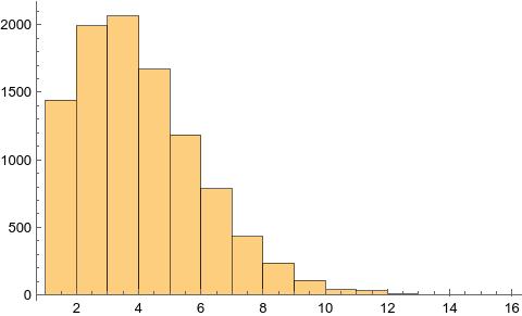
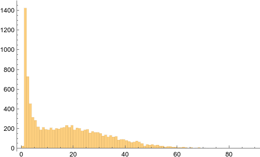
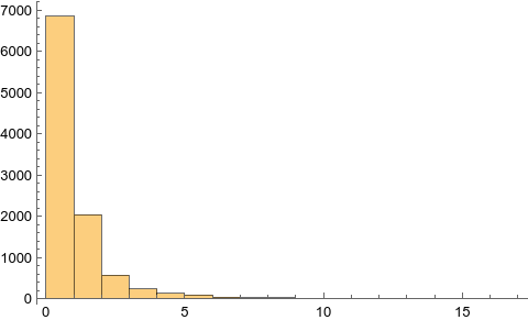
For , the total number of leaves is infinite with a positive probability. Consequently, for each . It is conceivable that the histogram of should also have a heavy tail. The hyperexplosive nature of the tree makes direct simulations of challenging. To mitigate this, a truncation of is simulated. Let be the subset of vertices of heights less than or equal to , and . Then by conditioning on , one may easily see that
and as . Here, is a mean-one exponential random variable, and and are two i.i.d. copies of . Figures 1a, 2a, 3a show the histograms of with 10000 experiments in the cases , , and , respectively. The heavy tail in the case is consistent with the “weak” hyperexplosive behavior of the random tree, i.e. .
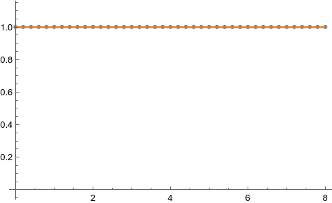
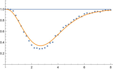
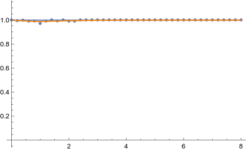
In the second set of figures, we simulate the function , which is the probability of getting finitely many -leaves. This function solves the -Riccati equation with the initial data . According to (2.1), is the pointwise limit of and
One can interpret this recursion probabilistically as where
| (3.1) |
and . To get (approximately) , observe that it is the maximal solution to the equation
and thus is the limit of the sequence , where
| (3.2) |
and . Now for the simulation of , we discretize the time interval and simulate the approximation at each grid point via a Monte Carlo algorithm using (3.1), where the initial process is approximated by , obtained analytically from (3.2). Figures 1b, 2b, 3b illustrate in the cases , , and , respectively. The dots are the numerical results obtained by Monte Carlo simulation. The orange curves are the Bézier curves fitting the data.
Various numerical solutions to the equation were computed by Nick Hale and André Weideman at Stellenbosch University, South Africa, using a different numerical method than that presented here (personal communication). In the range , one of their curves has a similar profile as that for in Figure 2b. Not all of these numerical solutions are explained by the current theory.
References
