m o \IfNoValueTF#2 p(#1)p(#1 — #2)
The stress-free state of human erythrocytes: data driven inference of a transferable RBC model
Abstract
The stress-free state (SFS) of red blood cells (RBCs) is a fundamental reference configuration for the calibration of computational models, yet it remains unknown. Current experimental methods cannot measure the SFS of cells without affecting their mechanical properties while computational postulates are the subject of controversial discussions. Here, we introduce data driven estimates of the SFS shape and the visco-elastic properties of RBCs. We employ data from single-cell experiments that include measurements of the equilibrium shape, of stretched cells, and relaxation times of initially stretched RBCs. A hierarchical Bayesian model accounts for these experimental and data heterogeneities. We quantify, for the first time, the SFS of RBCs and use it to introduce a transferable RBC (t-RBC) model. The effectiveness of the proposed model is shown on predictions of unseen experimental conditions during the inference, including the critical stress of transitions between tumbling and tank-treading cells in shear flow. Our findings demonstrate that the proposed t-RBC model provides predictions of blood flows with unprecedented accuracy and quantified uncertainties.
Introduction
RBC are vital elements of blood as they are responsible for the delivery of oxygen to the entire human body. As they traverse the microcirculature red blood cells undergo highly non-linear deformations, that are accommodated by their visco-elastic properties [2]. These properties are mainly controlled by the structure of their membrane, composed of a lipid bilayer anchored on a network of proteins (cytoskeleton), and enclosing a viscous solvent (hemoglobin). The RBC membrane and the hemoglobin are both considered incompressible. The cytoskeleton and the lipid bilayer of the membrane provide elastic resistance against local shearing, stretching, and bending. Over the last two decades numerous mathematical models for the RBC membrane have been proposed, aiming to explain complex phenomena, and complement experimental studies through parametric exploration and system optimization [3].
State-of-the-art models of RBCs account for shear deformation of the membrane with respect to a state at which the membrane has zero in-plane elastic energy, namely the stress free state (SFS) [4, 5, 6, 7, 8, 9]. The existence of a non-spherical SFS was demonstrated by the experimental results of Fischer [10], who showed that the RBC membrane exhibits shape memory, and of Dupire et al. [11], who suggested that shape memory can explain certain dynamical transitions of cells in shear flow. Švelc and Svetina [12] suggested an analysis to compare the deformation of the cytoskeleton in a micropipette for a given SFS shape to that measured by experiments [13], but did not infer the SFS from the experimental data. Furthermore, current experimental methods do not allow to directly measure the SFS of cells without affecting their mechanical properties (see section 2.3.3 of Lim H. W. et al. [4] and references therein). For these reasons, previous works have performed parametric studies using a predefined SFS. Such calibrations affect the dynamics of RBCs, and in turn are key factors when comparing computational and experimental data [14, 6, 7, 15, 4]. An ever increasing amount of evidence from both experiments and simulations have shown that the SFS of the membrane skeleton is neither the biconcave resting shape, nor a spherical shell [6, 7, 15]. The consensus on the SFS is an oblate-like shell, with the same surface area and a larger volume than the RBC, though the exact SFS remains elusive [14, 6, 7].
Several computational studies have performed parametric investigations to quantify the effect of the SFS on the response of RBCs, under static and dynamic conditions [16, 4, 15, 6, 7, 17]. The SFS calibration shape was shown to significantly affect predictions of the RBC dynamics in simple shear flow. In particular, computational findings [6, 7] demonstrated that the SFS alters not only the critical shear rate separating tumbling and tank-treading RBC dynamics, but also the motion of the RBC membrane at the critical shear rate. Peng et al. [7] searched for a family of SFSs, which could reproduce at the same time the biconcave resting shape and the dynamics of single erythrocytes in simple shear flow. Their findings show that a SFS closer to a sphere, rather than to a biconcave disk, approaches not only the experimental critical shear stress, but also preserves the experimentally observed biconcave shape during tank-treading [11]. This finding was in contrast to previous computational studies. As a result, Peng et al. [7] envisioned that RBC dynamics at low shear rates might enable the quantification of the SFS.
We complement the aforementioned studies, by performing a data-driven inference of the SFS and its potential variability in the population of healthy RBCs. We use hierarchical Bayesian inference to integrate data from multiple experimental sources and conditions, and generate a data-informed probabilistic RBC model that incorporates modeling and experimental uncertainties in its predictions [1]. The structure of the model incorporates the variability [18] of RBCs elastic properties. In contrast to the recent study by Economides et al. [1], where the RBC model was considered a “black-box” with an arbitrary, predefined SFS, here we perform a global sensitivity analysis for each quantity of interest. Inert factors are excluded during the inference process, to reduce the computational cost and avoid numerical artifacts while sampling the posterior distribution [19]. The high computational cost associated with the Bayesian inference is mitigated by the use of neural networks as emulators of the RBC model output. This approach enables the simultaneous inference of all material properties in the employed RBC model. In particular, the SFS (parameterized by its reduced volume), shear (both linear and non-linear components), and bending moduli are inferred from experimental data of RBCs in equilibrium [20], and under stretching [21, 22]. In turn, the membrane viscosity is inferred from experiments of RBC relaxation after elongation [23].
Predictions of the fully-calibrated model are validated against experimental data coming from complex flow conditions that were not part of the inference. Specifically, the calibrated model captures the velocity and elongation of RBCs flowing in a microtube [24], the tank treading frequency (TTF) and inclination angle of RBCs in simple shear flows [25], and, most importantly, the critical shear stress between the tumbling and tank-treading motion of RBCs in shear flow [26]. Our findings demonstrate, for the first time, the transferability of the inferred model, without problem specific tuning, and its capability to predict complex flow configurations that were not part of the inference.
Methods
Red Blood Cell model
We model the RBC membrane as a surface whose dynamics evolve according to bending resistance of the lipid-bilayer, shear and dilation elasticity of the cytoskeleton and membrane viscosity. The shear and dilation elasticity are minimal at the SFS of the RBC, a state that is not known. The resistance to bending is described by the energy
| (1) |
where the integral is taken over the membrane, is the bending modulus and is the mean curvature of the membrane. The in-plane elastic energy accounts for the shear and dilation elasticity of the cytoskeleton,
| (2) |
where the integral is taken over the SFS surface, and are the local dilation and shear strain invariants of the membrane, respectively, is the dilation elastic modulus, is the shear elastic modulus and the coefficients , , and are parameters that control the non-linearity of the membrane elasticity for large deformations [4].
The membrane is discretized into a triangle mesh composed of vertices with positions , velocities and mass , , evolving according to Newton’s law of motion. The bending energy described by eq. 1 is discretized following Jülicher [27], Bian et al. [28] and the in-plane energy is computed as described in Lim H. W. et al. [4]. The forces arising from these energy terms are formed by the negative gradient of the energy with respect to the particle positions. The membrane viscosity is modeled through pairwise forces between particles sharing an edge in the triangle mesh. The viscous force exerted by particle to particle is given by [29]
| (3) |
where is the friction coefficient, and is the unit vector between to . The membrane viscosity depends linearly on the friction coefficient, . Finally, the constraints of preserving the area of the membrane and the volume of the cytosol are enforced through energy penalization terms,
where and are the area and volume of the cell at rest and and are the area and volume of the cell, respectively. The coefficients and are chosen empirically with values that are large enough to enforce the conservation of the membrane area and volume of the RBC. More details on the discretization of the energies are presented in the supplementary material.
The SFS of the RBC is parameterized by its reduced volume , i.e., the volume of the SFS relative to that of a sphere with same area as the SFS. Following Lim H. W. et al. [4], the SFS is obtained by minimizing the energy of a membrane with bending resistance, shear and dilation elastic energy with a sphere as reference state. The area of the SFS is constrained to that of a healthy RBC and the volume is parameterized by the reduced volume (ratio of the volume with respect to that of a sphere with the same area). With ranging from 0.65 to unity, this procedure results in biconcave shapes, oblates and spheroids at low, intermediate and high reduced volume, respectively (fig. 1). We note that the value of this reduced volume is chosen arbitrarily in RBC models and accordingly affects their dynamics.

The parameters governing the RBC mechanics comprise the reduced volume of the SFS , the shear modulus , the shear-hardening coefficient , the bending modulus and the membrane viscosity . These parameters are calibrated from experimental data sets that we introduce in the next sections. The remaining parameters of the model are chosen as follows: the dilation elastic modulus is set to ; the non-linear coefficients in the shear energy formulation are set to , and [4]; the area and volume of the cells are fixed to and , respectively [20].
Heterogeneous data and a probabilistic model for the RBC: t-RBC
We link seven experimental data sets measured from three experimental conditions with the computational model using a hierarchical statistical framework. The first data set corresponds to the measurements of the diameter , maximal thickness and minimal thickness of single cells at equilibrium, as reported by Evans and Fung [20]. The second and third data sets are measurements of the two principal diameters of RBCs stretched by two micro-beads. The micro-beads are attached to the membrane at two opposite sides of the cell’s rim and are pulled by forces of magnitude in opposite directions. The two largest principal diameters of the cells, and , are reported by Mills et al. [21] and Suresh et al. [22] against the stretching force magnitude . The remaining data sets were collected by Hochmuth et al. [23] from initially stretched RBCs relaxing to their equilibrium shape. The data sets consist in the ratio of the two principal diameters of the cells, measured at constant time intervals.
We assume that each data set is one realization of the random variable (called observable), where denotes the experimental conditions (equilibrium, stretching or relaxation) and is the index of the data set (we drop the indices in the remaining of this section to lighten the notations). The t-RBC model relates the computational model and its parameters to the probability distribution of the observable. The structure of the t-RBC model, represented as a directed acyclic graph (DAG), is shown on fig. 2. We distinguish the parameters of the computational model, , from those of the error model (explained below) such as the standard deviation . In addition, we introduce the hyper-parameter that is further discussed below.
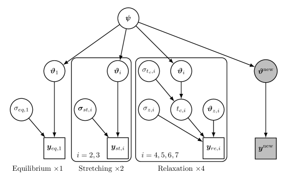
The hierarchical structure of the t-RBC model represents two levels of uncertainty. First, the computational parameters for each data set is drawn from a distribution parameterized by the hyper parameter , , representing the variability of the cells properties. This variability is due to the origin of the cells (from different donors), the age of the cells and the different experimental conditions. Second, for each data set, the observable is assumed to be normally distributed around the output of the computational model. This second level of uncertainty reflects the measurement errors and the inaccuracy of the computational model. The measurements errors are modeled separately for each experimental conditions, with parameters as shown in fig. 2. We note that in the case of the relaxation experiment, we introduced an intermediate variable, , which is the relaxation time of the cell. This addition simplifies the inference procedure as the initial shape of the RBC in experiments is unknown. Instead, we assume that depends on the RBC parameters only and is independent on the initial shape of the cell. This assumption allows to estimate from the computational model with an arbitrary initial stretched shape. The data is then modeled as an exponential decay with rate and additional parameters contained in . The exact dependencies between the random variables are detailed in the supplementary material.
Offline surrogate of the computational model
The evaluation of the computational model for each experimental condition (cell equilibration, stretching and relaxation), while relatively fast thanks to the high-performance implementation in Mirheo [30], remains computationally costly for performing Bayesian inference of the t-RBC model presented above. Instead, we replace the computational model during the Bayesian inference with an offline surrogate.

The surrogate is formed by three NNs, one for each experimental condition, that takes as input the computational parameters (and the stretching force magnitude for the stretching case) and outputs the observable of the computational model ( for the equilibration case, for the stretching case and for the relaxation case). Each NN is composed of three hidden layers of 32 neurons and hyperbolic tangent activation gates. The training data was generated for 50’000 samples uniformly distributed in the input space of the surrogate. The corresponding observable values were then computed with the procedure described in fig. 3 using the computational model. The NN parameters were then trained on these samples (split into 80% and 20% training and validation sets, respectively) to minimize the mean squared error between the NNs and the computational model. The training was performed with the Adam optimizer and we used early stopping to avoid over-fitting. The prediction accuracy of the surrogate is shown in the supplementary material.
Results and Discussion
Bayesian Inference
We infer the parameters of the RBC model from the combined experimental data sets using hierarchical Bayesian inference. The posterior distribution of the parameters is sampled using Bayesian annealed sequential important sampling (BASIS) [31], an unbiased version of transitional Markov chain Monte-Carlo (TMCMC) [32]. This sampling method does not rely on the gradient of the model with respect to the parameters. In this situation, regions of constant likelihood lead to poor sampling [33]. In turn, we eliminate the parameters that are inert for the respective experimental condition. We performed a sensitivity analysis of the model output with respect to the parameters in the supplementary material. The results indicate that the combination of the three experimental cases chosen in this study are complementary for the inference of the cell parameters: the equilibrium shape is sensitive to and (where is the Föppl-von Kármánn number), the stretched cell diameters vary mainly with and (and and at low stretching forces) and the relaxation characteristic time is sensitive to and .
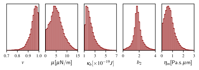
The parameters of the t-RBC model are sampled as described in the supplementary material using the Korali framework [34]. The resulting posterior distribution of the RBC parameters, , is shown on fig. 4, with corresponding mean, median, maximum likelihood (ML) and maximum a posteriori (MAP) values reported in table 1. All distributions have a clear peak with relatively high uncertainties around the MAP, due to the heterogeneity of the data sets.
The inferred shear modulus has a mean at , which is within the range of values used in previous studies: [35, 36], [37], [38]. Similarly, the inferred bending modulus is consistent with the values used in previous works ( [35], [36], [37], [38]). In addition, the inferred membrane viscosity is close to that found in Wälchli et al. [39] () and in Hochmuth et al. [23] (). The parameter is found higher than in Lim H. W. et al. [4] (). However, the cell deformations were most likely smaller in the latter study than in the cell-stretching experiments that were used for the inference.
The inferred reduced volume of the SFS has a mean around , which suggests that the SFS is more likely an oblate than the biconcave shape, based on these experimental data sets. This value is close to those used in previous studies ( [5], [9], [7, 8], [6]). Furthermore, the range of values obtained from the Bayesian inference agrees with the conclusions of Lim H. W. et al. [4], who showed that to reproduce the stomatocyte-discocyte-echinocyte (SDE) sequence observed when changing the bending properties of the lipid-bilayer of the membrane. Similarly, Geekiyanage et al. [40] concluded that the reduced volume of the SFS is around to obtain the SDE sequence. We note that the result of Lim H. W. et al. [4] was obtained with predefined values of the mechanical properties of the membranes, while in the current work the mechanical properties of the membranes are inferred together with the SFS reduced volume. Furthermore, the studies that inferred the SFS reduced volume based on the SDE sequence did not consider the dynamics of the RBCs in dynamic flow conditions [4, 40],
| mean | median | ML | MAP | standard deviation | |
|---|---|---|---|---|---|
| 0.94 | 0.95 | 0.96 | 0.96 | 0.04 | |
| 4.99 | 4.68 | 4.60 | 4.60 | 2.24 | |
| 2.10 | 1.85 | 1.46 | 1.46 | 0.93 | |
| 1.84 | 1.73 | 1.69 | 1.69 | 0.82 | |
| 0.69 | 0.62 | 0.66 | 0.66 | 0.46 |
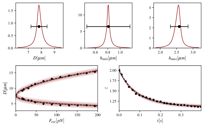
The inferred parameters are then tested against the experimental data sets used for the inference. Figure 5 shows the predictions of the t-RBC model for one data set for each experimental condition. The parameters used for the predictions are sampled from the probability distribution , where contains the seven data sets used for the inference. In all cases, the experimental data lie inside the credible intervals given by the t-RBC model.
Model generalization
Contrary to the one-at-a-time approach, a commonly used practice for validating RBC models [41, 42, 35], we test the predictive accuracy of the calibrated RBC model in configurations that were not seen during the inference. The posterior distribution of the parameters was inferred using simple experimental conditions where only one or two parameters had a significant effect on the output in each case. Here the calibrated model is validated in complex dynamic situations, where multiple parameters affect the output, as shown in parametric studies found in the literature (details below). In particular, we test the model prediction on five quantities: the TTF, inclination angle, and threshold shear stress for tumbling-to-tank-treading transition of RBCs in simple shear flow, the elongation of RBCs flowing through a microtube and their respective velocity against the applied pressure gradient. The TTF and inclination angle are known to be significantly affected by the membrane viscosity [43]. The threshold shear stress for tumbling-to-tank-treading transition depends on the SFS [6, 7], and the length of flowing RBCs in microtubes depends on the bending stiffness of the membrane [44]. We emphasize that it is crucial to estimate the prediction capabilities of the model on data coming from conditions not seen during the inference phase to test the transferability of the model.
The following cases are substantially more expensive in terms of computations than those used to calibrate the model (each evaluation takes at least 24 hours on a single P100 graphics processing unit). Therefore, instead of propagating the posterior distribution of the parameters through the computational model, we evaluate each quantity of interest with the mean estimates of the posterior distribution.
RBC in a circular microtube
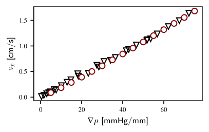
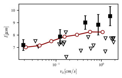
Single RBCs flowing in straight microtubes adopt a steady parachute-like shape. The cell length and velocity depend on the flow rate and the radius of the tube. A pressure difference between the ends of the tube causes the solvent and the cell to flow. The tube has a length large enough so that the cells reach an equilibrium shape before the measurements. The length and velocity of the cells, and , were recorded for different pressure gradients experimentally for [24] and [45]. Simulations of this system are performed with the current calibrated model (using the mean of the posterior distributions) for (see supplementary material for details). The simulations show a good agreement with the experimental data (fig. 6). The variability of the cell lengths in the experiments could be attributed to the variability in the mechanical properties of the cells, but also to that of the cell sizes.
RBC in a linear shear flow
Single RBCs suspended in a linear shear flow exhibit rich dynamics. At low shear rates, the cells tumble (rotate in a rigid-like motion). Increasing the shear rate above a threshold value causes the cell membrane to tank tread: the cell adopts an elongated shape forming an angle with the flow direction, while the membrane rotates around the cell with a frequency (the TTF). Below we present predictions of the t-RBC model for the inclination angle, the TTF and the critical shear stress for tumbling to tank-treading transition. These predictions were obtained for a fixed cytosol viscosity (see supplementary material). However, we remark that this quantity is known to depend on the hemoglobin concentration, which varies notably with the age of the cells, and it may be of importance to model this variation in further research [46].
Inclination angle.

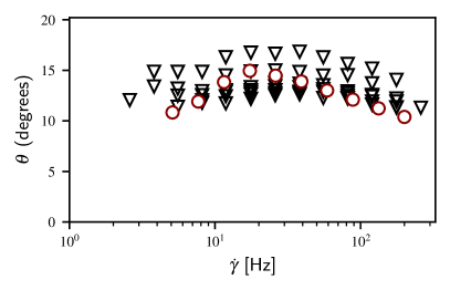
Measurements of inclination angles of tank-treading RBCs in simple shear flows have been reported by Fischer and Korzeniewski [25]. The inclination angle obtained with the calibrated RBC model (with the mean estimate of the parameters) is shown against the shear rate on fig. 7. The model predictions are within the values observed experimentally. In particular, for a solvent viscosity , the model captures the trend of the experimental data, i.e. an increase of with followed by a decrease of above a critical shear rate. This trend is less pronounced at the lower solvent viscosity , both experimentally and in the simulations.
Tank treading frequency.
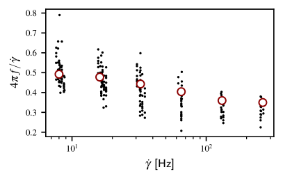
Figure 8 shows the dimensionless TTF, , of a tank-treading RBC suspended in a linear shear flow (with solvent viscosity ) for various shear rates . The t-RBC model predictions are performed with the mean estimate of the parameters. Despite the complex dependency of the TTF on the computational parameters, the t-RBC model shows a good agreement with the TTF experimental data reported by Fischer [47]. Furthermore, the biconcave shape of the cell is preserved in the tank-treading simulations, as observed experimentally [11] (see fig. S2). However, we note that the biconcavity of the cell during tank treading is only reported qualitatively in experiments, and quantitative experimental data could help improving further the calibration of the model.
Tumbling to tank-treading transitions in linear shear flow.
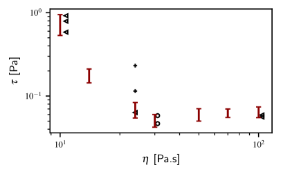
RBC in a linear shear flow undergo different regimes depending on the shear rate and solvent viscosity [49]. At large shear rates, the cell orientation oscillates around a steady angle while the membrane rolls, or “tank-treads” around the cell. In contrast, RBCs rotate as a rigid object, or “tumble”, when the shear rate is below a critical value. The critical shear stress has been measured experimentally by Abkarian et al. [48] and Fischer and Korzeniewski [26] for different solvent viscosity . We performed numerical simulations with the calibrated model at different shear rates for several viscosity values . For a given solvent viscosity, the flow regime of the cell (tumbling or tank-treading) was reported for several shear rates. The highest and lowest shear rates at which the RBC tumbles and tank-treads, respectively, are reported on fig. 8. The model predictions are in good agreement with experimental data. As in the experimental data, the critical shear stress decreases sharply for solvent viscosity below and reaches a plateau above that viscosity. Note that we show only the transitions for the discocytes in the data from Fischer and Korzeniewski [26]. The data points marked with crosses at are from cells that previously underwent shape transitions, possibly modifying their mechanical properties. This observation probably explains the deviations between the shear stress obtained from experiments and that obtained from the simulations at this particular viscosity.
Limitations
To minimize the computational cost of inference, we have fixed several parameters to specific values. Specifically, the membrane model assumes zero spontaneous curvature (eq. 1), which typically results from differences in monolayer compositions found in-vivo. However, discocytes, as shown in Figure 2.45 of Lim H. W. et al. [4], have been found to exhibit a spontaneous curvature close to zero and we therefore ignored the spontaneous curvature in the current work. Similarly, the area and volume of the RBCs exhibit a distribution that reflects the variability and aging of the cells. While it is possible to include these variations in the statistical model, doing so would increase the complexity of the model and the computational cost for inference. For similar reasons, we fixed the ratio as in Economides et al. [1]. While this choice is arbitrary, the current model predicts accurately various flow conditions. The value of these parameters should ideally be inferred from additional experimental data and can be the subject of future research.
Conclusion
We introduce a transferable RBC model (t-RBC) that quantifies the visco-elastic membrane parameters and the SFS of healthy RBCs through Bayesian inference. The t-RBC model takes into account the cell heterogeneity, the measurement errors and the computational model inaccuracies. The model parameters were calibrated on 7 data sets comprising measurements of RBC dimensions at equilibrium, RBC elongation under stretching forces and RBC relaxation time. The posterior distribution of the parameters have a relatively large standard deviation that possibly reflects the variability of mechanical properties among RBCs. The reduced volume of the SFS takes values that suggest that the cytoskeleton of RBCs, in its unstressed state, has an oblate shape. The calibrated shear modulus, bending modulus and viscosity of the membrane were found to be in good agreement with previous studies, and we provide uncertainty on these parameters.
The calibrated model predicts accurately complex, single-cell dynamics, and agrees well with experimental data that were not used during the inference phase. In particular, the calibrated model predicts accurately the velocity and length of cells flowing in narrow tubes, the inclination angle and TTF of tank-treading cells in linear shear flows, and the critical shear stress of the tumbling to tank-treading motion of RBCs in linear shear flows. We emphasize that the aforementioned quantities highly depend on the visco-elastic properties of the RBC model, as demonstrated in numerous parametric studies in the literature. The transferability of the proposed t-RBC model makes it a candidate of choice for predicting the dynamics of RBCs in previously unseen flow configurations that involve large deformations and/or complex dynamics. In addition, the variability of the inferred parameters can be used to provide a more realistic description of blood flows with many cells, each cell having parameters drawn from the posterior density. This approach would model the heterogeneity of the cells in blood. The samples from the posterior density of the parameters are available online, together with the code used to produce the results of this study [50].
Author Contributions
AE, LA, PK designed the research. LA, AE ran the RBC simulations. LA, AE, GA performed the Bayesian inference. LA built the surrogate model. LA, AE, PK interpreted the results. LA, AE, GA, PK wrote the article.
Acknowledgments
We would like to thank Xin Bian and Sergey Litvinov for their invaluable insights on RBC modeling and simulations. We acknowledge support by the The European High Performance Computing Joint Undertaking (EuroHPC) Grant DComEX (956201-H2020-JTI-EuroHPC-2019-1), and computational resources granted by the Swiss National Supercomputing Center (CSCS) under the project ID “s929”.
Declaration of Interest
The authors declare no competing interests.
References
- Economides et al. [2021] Economides, A., G. Arampatzis, D. Alexeev, S. Litvinov, L. Amoudruz, L. Kulakova, C. Papadimitriou, and P. Koumoutsakos, 2021. Hierarchical Bayesian Uncertainty Quantification for a Model of the Red Blood Cell. Physical Review Applied 15:034062.
- Caro et al. [2011] Caro, C. G., T. J. Pedley, R. C. Schroter, W. A. Seed, and K. H. Parker, 2011. The mechanics of the circulation. Cambridge University Press, Cambridge, second edition.
- Freund [2014] Freund, J. B., 2014. Numerical Simulation of Flowing Blood Cells. Annual Review of Fluid Mechanics 46:67–95.
- Lim H. W. et al. [2008] Lim H. W., G., M. Wortis, and R. Mukhopadhyay, 2008. Red Blood Cell Shapes and Shape Transformations: Newtonian Mechanics of a Composite Membrane. Soft Matter 4.
- Khairy et al. [2008] Khairy, K., J. Foo, and J. Howard, 2008. Shapes of red blood cells: comparison of 3D confocal images with the bilayer-couple model. Cellular and molecular bioengineering 1:173–181.
- Cordasco et al. [2014] Cordasco, D., A. Yazdani, and P. Bagchi, 2014. Comparison of erythrocyte dynamics in shear flow under different stress-free configurations. Physics of Fluids 26.
- Peng et al. [2014] Peng, Z., A. Mashayekh, and Q. Zhu, 2014. Erythrocyte responses in low-shear-rate flows: Effects of non-biconcave stress-free state in the cytoskeleton. Journal of Fluid Mechanics 742:96–118.
- Peng et al. [2015] Peng, Z., S. Salehyar, and Q. Zhu, 2015. Stability of the tank treading modes of erythrocytes and its dependence on cytoskeleton reference states. Journal of Fluid Mechanics 771:449–467.
- Mauer et al. [2018] Mauer, J., S. Mendez, L. Lanotte, F. Nicoud, M. Abkarian, G. Gompper, and D. A. Fedosov, 2018. Flow-Induced Transitions of Red Blood Cell Shapes under Shear. Phys. Rev. Lett. 121:118103–1–6.
- Fischer [2004] Fischer, T. M., 2004. Shape Memory of Human Red Blood Cells. Biophysical Journal 86:3304–3313.
- Dupire et al. [2012] Dupire, J., M. Socol, and A. Viallat, 2012. Full dynamics of a red blood cell in shear flow. Proceedings of the National Academy of Sciences of the United States of America 109:20808.
- Švelc and Svetina [2012] Švelc, T., and S. Svetina, 2012. Stress-free state of the red blood cell membrane and the deformation of its skeleton. Cellular and Molecular Biology Letters 17:217–227.
- Lee et al. [1999] Lee, J. C., D. T. Wong, and D. E. Discher, 1999. Direct measures of large, anisotropic strains in deformation of the erythrocyte cytoskeleton. Biophysical journal 77:853–864.
- Levant and Steinberg [2016] Levant, M., and V. Steinberg, 2016. Intermediate regime and a phase diagram of red blood cell dynamics in a linear flow. Physical Review E 94:1–14.
- Tsubota et al. [2014] Tsubota, K. I., S. Wada, and H. Liu, 2014. Elastic behavior of a red blood cell with the membrane’s nonuniform natural state: Equilibrium shape, motion transition under shear flow, and elongation during tank-treading motion. Biomechanics and Modeling in Mechanobiology 13:735–746.
- Li et al. [2005] Li, J., M. Dao, C. Lim, and S. Suresh, 2005. Spectrin-level modeling of the cytoskeleton and optical tweezers stretching of the erythrocyte. Biophysical journal 88:3707–3719.
- Cordasco and Bagchi [2017] Cordasco, D., and P. Bagchi, 2017. On the shape memory of red blood cells. Physics of Fluids 29:1–18.
- Reichel et al. [2019] Reichel, F., J. Mauer, A. A. Nawaz, G. Gompper, J. Guck, and D. A. Fedosov, 2019. High-throughput microfluidic characterization of erythrocyte shapes and mechanical variability. Biophysical journal 117:14–24.
- Arampatzis et al. [2018] Arampatzis, G., D. Walchli, P. Angelikopoulos, S. Wu, P. Hadjidoukas, and P. Koumoutsakos, 2018. Langevin diffusion for population based sampling with an application in Bayesian inference for pharmacodynamics. SIAM Journal on Scientific Computing 40:B788–B811.
- Evans and Fung [1972] Evans, E., and Y. C. Fung, 1972. Improved measurements of the erythrocyte geometry. Microvascular Research 4:335–347.
- Mills et al. [2004] Mills, J. P., L. Qie, M. Dao, C. T. Lim, S. Suresh, and Others, 2004. Nonlinear elastic and viscoelastic deformation of the human red blood cell with optical tweezers. MCB-TECH SCIENCE PRESS- 1:169–180.
- Suresh et al. [2005] Suresh, S., J. Spatz, J. P. Mills, A. Micoulet, M. Dao, C. T. Lim, M. Beil, and T. Seufferlein, 2005. Connections between single-cell biomechanics and human disease states: Gastrointestinal cancer and malaria. Acta Biomaterialia 1:15–30.
- Hochmuth et al. [1979] Hochmuth, R. M., P. R. Worthy, and E. A. Evans, 1979. Red cell extensional recovery and the determination of membrane viscosity. Biophysical Journal 26:101–114.
- Tomaiuolo et al. [2009] Tomaiuolo, G., M. Simeone, V. Martinelli, B. Rotoli, and S. Guido, 2009. Red blood cell deformation in microconfined flow. Soft Matter 5:3736–3740.
- Fischer and Korzeniewski [2015] Fischer, T. M., and R. Korzeniewski, 2015. Angle of inclination of tank-treading red cells: Dependence on shear rate and suspending medium. Biophysical Journal 108:1352–1360.
- Fischer and Korzeniewski [2013] Fischer, T. M., and R. Korzeniewski, 2013. Threshold shear stress for the transition between tumbling and tank-treading of red blood cells in shear flow: dependence on the viscosity of the suspending medium. Journal of fluid mechanics 736:351–365.
- Jülicher [1996] Jülicher, F., 1996. The morphology of vesicles of higher topological genus: conformal degeneracy and conformal modes. Journal de Physique II 6:1797–1824.
- Bian et al. [2020] Bian, X., S. Litvinov, and P. Koumoutsakos, 2020. Bending models of lipid bilayer membranes: Spontaneous curvature and area-difference elasticity. Comput. Method. Appl. M. 359:112758.
- Fedosov [2010] Fedosov, D. A., 2010. Multiscale modeling of blood flow and soft matter. Ph.D. thesis, Citeseer.
- Alexeev et al. [2020] Alexeev, D., L. Amoudruz, S. Litvinov, and P. Koumoutsakos, 2020. Mirheo: High-performance mesoscale simulations for microfluidics. Comput. Phys. Commun. 107298.
- Wu et al. [2017] Wu, S., P. Angelikopoulos, C. Papadimitriou, and P. Koumoutsakos, 2017. Bayesian Annealed Sequential Importance Sampling (BASIS): an unbiased version of Transitional Markov Chain Monte Carlo. ASCE-ASME J. Risk Uncertain. Eng. Sys. B .
- Ching and Chen [2007] Ching, J., and Y.-C. Chen, 2007. Transitional Markov chain Monte Carlo method for Bayesian model updating, model class selection, and model averaging. Journal of engineering mechanics 133:816–832.
- Raue et al. [2013] Raue, A., C. Kreutz, F. J. Theis, and J. Timmer, 2013. Joining forces of Bayesian and frequentist methodology: a study for inference in the presence of non-identifiability. Philosophical Transactions of the Royal Society A: Mathematical, Physical and Engineering Sciences 371:20110544.
- Martin et al. [2021] Martin, S. M., D. Wälchli, G. Arampatzis, A. E. Economides, P. Karnakov, and P. Koumoutsakos, 2021. Korali: Efficient and scalable software framework for Bayesian uncertainty quantification and stochastic optimization. Comput. Method. Appl. M. 114264.
- Fedosov et al. [2010a] Fedosov, D. A., B. Caswell, and G. E. Karniadakis, 2010. Systematic coarse-graining of spectrin-level red blood cell models. Computer Methods in Applied Mechanics and Engineering 199:1937–1948.
- Fedosov et al. [2010b] Fedosov, D. A., B. Caswell, and G. E. Karniadakis, 2010. A multiscale red blood cell model with accurate mechanics, rheology, and dynamics. Biophysical journal 98:2215–2225.
- Turlier et al. [2016] Turlier, H., D. A. Fedosov, B. Audoly, T. Auth, N. S. Gov, C. Sykes, J.-F. Joanny, G. Gompper, and T. Betz, 2016. Equilibrium physics breakdown reveals the active nature of red blood cell flickering. Nature physics 12:513–519.
- Yazdani and Karniadakis [2016] Yazdani, A., and G. E. Karniadakis, 2016. Sub-cellular modeling of platelet transport in blood flow through microchannels with constriction. Soft Matter 12:4339–4351.
- Wälchli et al. [2020] Wälchli, D., S. M. Martin, A. Economides, L. Amoudruz, G. Arampatzis, X. Bian, and P. Koumoutsakos, 2020. Load Balancing in Large Scale Bayesian Inference. In Proceedings of the Platform for Advanced Scientific Computing Conference – PASC '20. ACM.
- Geekiyanage et al. [2019] Geekiyanage, N. M., M. A. Balanant, E. Sauret, S. Saha, R. Flower, C. T. Lim, and Y. Gu, 2019. A coarse-grained red blood cell membrane model to study stomatocyte-discocyte-echinocyte morphologies. PLoS One 14:e0215447.
- Kotsalos et al. [2019] Kotsalos, C., J. Latt, and B. Chopard, 2019. Bridging the computational gap between mesoscopic and continuum modeling of red blood cells for fully resolved blood flow. Journal of Computational Physics 398:108905.
- Dupin et al. [2007] Dupin, M. M., I. Halliday, C. M. Care, L. Alboul, and L. L. Munn, 2007. Modeling the flow of dense suspensions of deformable particles in three dimensions. Physical Review E - Statistical, Nonlinear, and Soft Matter Physics 75:1–17.
- Yazdani and Bagchi [2013] Yazdani, A., and P. Bagchi, 2013. Influence of membrane viscosity on capsule dynamics in shear flow. Journal of Fluid Mechanics 718:569–595.
- Noguchi and Gompper [2005] Noguchi, H., and G. Gompper, 2005. Shape transitions of fluid vesicles and red blood cells in capillary flows. Proceedings of the National Academy of Sciences 102:14159–14164.
- Hochmuth et al. [1970] Hochmuth, R., R. Marple, and S. Sutera, 1970. Capillary blood flow: I. Erythrocyte deformation in glass capillaries. Microvascular research 2:409–419.
- Chien et al. [1970] Chien, S., S. Usami, J. F. Bertles, et al., 1970. Abnormal rheology of oxygenated blood in sickle cell anemia. The Journal of clinical investigation 49:623–634.
- Fischer [2007] Fischer, T. M., 2007. Tank-Tread Frequency of the Red Cell Membrane : Dependence on the Viscosity of the Suspending Medium. Biophysical Journal 93:2553–2561.
- Abkarian et al. [2007] Abkarian, M., M. Faivre, and A. Viallat, 2007. Swinging of red blood cells under shear flow. Physical Review Letters 98:2–5.
- Yazdani and Bagchi [2011] Yazdani, A. Z., and P. Bagchi, 2011. Phase diagram and breathing dynamics of a single red blood cell and a biconcave capsule in dilute shear flow. Physical Review E 84:026314.
- Amoudruz [2022] Amoudruz, L., 2022. cselab/tRBC-UQ: v1.0.0. https://doi.org/10.5281/zenodo.7320187.