Data-driven Modified Nodal Analysis Circuit Solver

Abstract

This work introduces a novel data-driven modified nodal analysis (MNA) circuit solver. The solver is capable of handling circuit problems featuring elements for which solely measurement data are available. Rather than utilizing hard-coded phenomenological model representations, the data-driven MNA solver reformulates the circuit problem such that the solution is found by minimizing the distance between circuit states that fulfill Kirchhoff’s laws, to states belonging to the measurement data. In this way, the previously inevitable demand for model representations is abolished, thus avoiding the introduction of related modeling errors and uncertainties. The proposed solver is applied to linear and nonlinear RC-circuits and to a half-wave rectifier.

I Introduction

Circuit simulations play a key role in the design and optimization process of electrical devices. To solve circuit problems, two types of equations are necessary. On the one hand, there are Kirchhoff’s laws, which are derived from first principles and are accepted as exactly known [21]. On the other hand, there are model descriptions that represent the actual element behavior, which are essential in classical circuit solvers. These models are mostly empirically known, thus introducing errors and epistemic (model-form) uncertainties arising from the modeling process [28]. Very commonly, these models are obtained via data-fitting techniques, e.g., based on physically motivated approaches [26, 20] or sophisticated machine learning regression methods [15, 7, 19], to name a few options.

Nowadays, the availability of data increases steadily. For many circuit elements, the amount of behavioral data is unprecedentedly high, raising the opportunity for novel data-driven modeling and simulation methods. Under this light, data-driven computation has emerged as and grown into a research area of its own in recent years. A model-free data-driven approach was first proposed in [16, 17] for elasticity-related problems. Since then, the so-called data-driven computing framework has been extended to several problem classes as well [4, 18, 3, 11], including the authors’ contributions in the field of magnetic field simulation [8, 9, 10].

A common aspect in all aforementioned works is that the data-driven computing framework abolishes the previously inevitable need for model representations, e.g., regarding constitutive (material) laws. Instead, a double minimization problem is introduced to obtain the solution. Therein, the sought solution must simultaneously conform to the first-principle equations and be as close as possible to the provided measurement data. In this way, the simulation workflow is substantially reduced, as the problem at hand can be solved directly using the available measurement data, rather than investing effort in the development of model representations, which, even if considered to be adequate, remain empirical and inexact. Contrarily, using the data-driven computing framework, the modeling process and the associated errors and uncertainties are bypassed altogether.

This paper extends data-driven computation to the case of circuit solvers. In particular, a novel data-driven modified nodal analysis (MNA) [14] solver is introduced, which is able to resolve circuit problems where only data are available for certain circuit elements. Therein, some circuit elements are assumed to be exactly known, while only measurement data are available for the remaining elements. The MNA is then reformulated along the lines of the data-driven computing framework, such that a double minimization solver yields the states that conform to Kirchhoff’s laws, while also being as close as possible to the measurements. Three numerical experiments validate the data-driven MNA method, which is able to recover reference solutions obtained with standard MNA solvers. As would be expected, the solutions of the data-driven MNA solver become increasingly more accurate as the number of available measurements increases.

Note that the suggested data-driven MNA solver is completely different than other approaches that appear in the literature and which are also labeled as “data-driven” [1, 2, 5, 6, 12, 13, 22, 23, 29]. Specifically, the data-driven MNA solver does not rely on machine learning regression for computing circuit element models, which can then be used within standard circuit simulation tools. Instead, the suggested data-driven MNA solution method incorporates the measurement data directly into the solver and bypasses the element modeling step altogether.

The remaining of the paper is structured as follows. In Section II, we introduce the data-driven computing formulations in the MNA framework and derive the data-driven MNA circuit solver. Several numerical investigations are presented and discussed in Section III, namely for a linear RC-circuit, a nonlinear RC-circuit with a voltage-dependent capacitor, and a nonlinear half-wave rectifier. A discussion on the computational cost of the data-driven MNA solver is provided in Section IV. The paper is concluded with Section V, where we summarize our findings.

II Methodology

In this work we consider circuits that contain passive elements, i.e., resistors (G), capacitors (C) and inductors (L), voltage sources (V) and current sources (I). Let $\mathbf{A}_{X}\in\mathbb{R}^{(n-1)\times n_{\mathrm{X}}}$ denote the reduced incidence matrices of an arbitrary circuit, where $n$ denotes the number of nodes and $X\in\{\mathrm{G},\mathrm{C},\mathrm{L},\mathrm{V},\mathrm{I}\}$. Then, employing the MNA, Kirchhoff’s laws can be formulated as

$$\mathbf{A}_{\mathrm{G}}\mathbf{i}_{\mathrm{G}}(t)+\mathbf{A}_{\mathrm{C}}\dot{\mathbf{q}}_{\mathrm{C}}(t)+\mathbf{A}_{\mathrm{L}}\mathbf{i}_{\mathrm{L}}(t)+\mathbf{A}_{\mathrm{V}}\mathbf{i}_{\mathrm{V}}(t) =\mathbf{A}_{\mathrm{I}}\mathbf{i}_{\mathrm{src}}(t),$$ (1a)

$$\mathbf{A}_{\mathrm{G}}^{\top}\bm{\Phi}(t)-\mathbf{v}_{\mathrm{G}}(t) =0,$$ (1b)

$$\mathbf{A}_{\mathrm{C}}^{\top}\bm{\Phi}(t)-\mathbf{v}_{\mathrm{C}}(t) =0,$$ (1c)

$$\mathbf{A}_{\mathrm{L}}^{\top}\bm{\Phi}(t)-\dot{\bm{\Psi}}_{\mathrm{L}}(t) =0,$$ (1d)

$$\mathbf{A}_{\mathrm{V}}^{\top}\bm{\Phi}(t)-\mathbf{v}_{\mathrm{src}}(t) =0.$$ (1e)

Here, $\bm{\Phi}\in\mathbb{R}^{n-1}$ denotes the potential difference between the nodes and the mass node and $\mathbf{i}_{\mathrm{G}}\in\mathbb{R}^{n_{\mathrm{G}}},\,\mathbf{i}_{\mathrm{L}}\in\mathbb{R}^{n_{\mathrm{L}}},\,\mathbf{i}_{\mathrm{V}}\in\mathbb{R}^{n_{\mathrm{V}}},\,\mathbf{i}_{\mathrm{src}}\in\mathbb{R}^{n_{\mathrm{src}}}$ are the currents in branches with resistors, inductors, voltage sources, and current sources, respectively. The changes in charges and fluxes are denoted as $\dot{\mathbf{q}}_{\mathrm{C}}\in\mathbb{R}^{n_{\mathrm{C}}}$ and $\dot{\bm{\Psi}}_{\mathrm{L}}\in\mathbb{R}^{n_{\mathrm{L}}}$ respectively.

Applying a time-discretization scheme, e.g., the backward Euler method, the time-discrete counterpart of (1) reads

$$\mathbf{A}_{\mathrm{G}}\mathbf{i}^{n+1}_{\mathrm{G}}+h^{-1}\mathbf{A}_{\mathrm{C}}\mathbf{q}^{n+1}_{\mathrm{C}}$$

$$+\mathbf{A}_{\mathrm{L}}\mathbf{i}^{n+1}_{\mathrm{L}}+\mathbf{A}_{\mathrm{V}}\mathbf{i}^{n+1}_{\mathrm{V}} =\mathbf{A}_{\mathrm{I}}\mathbf{i}^{n+1}_{\mathrm{src}}+h^{-1}\mathbf{A}_{\mathrm{C}}\mathbf{q}_{\mathrm{C}}^{n},$$ (2a)

$$\mathbf{A}_{\mathrm{G}}^{\top}\bm{\Phi}^{n+1}-\mathbf{v}_{\mathrm{G}}^{n+1} =0,$$ (2b)

$$\mathbf{A}_{\mathrm{C}}^{\top}\bm{\Phi}^{n+1}-\mathbf{v}_{\mathrm{C}}^{n+1} =0,$$ (2c)

$$\mathbf{A}_{\mathrm{L}}^{\top}\bm{\Phi}^{n+1}-h^{-1}\bm{\Psi}^{n+1}_{\mathrm{L}} =h^{-1}\bm{\Psi}_{\mathrm{L}}^{n},$$ (2d)

$$\mathbf{A}_{\mathrm{V}}^{\top}\bm{\Phi}^{n+1}-\mathbf{v}_{\mathrm{src}}^{n+1} =0,$$ (2e)

where $h$ denotes the time step and $f^{n+1}=f(t+h)$, respectively, $f^{n}=f(t)$. To ease notation, we omit the superscript ⁿ⁺¹ in the following. All states that conform to Kirchhoff’s laws are collected in the set $\mathcal{K}=\{\bm{\zeta}:\bm{\zeta}=(\bm{\Phi},\mathbf{i}_{\mathrm{G}},\mathbf{q}_{\mathrm{C}},\bm{\Psi},\mathbf{i}_{\mathrm{L}},\mathbf{i}_{\mathrm{V}})\in\mathcal{Z}:\eqref{eq:KCL_time_discrete}\}$, where $\mathcal{Z}$ denotes the set of all possible states. For a traditional circuit solver, models for the circuits elements are needed to solve (2). The models’ responses can be collected in a set $\tilde{\mathcal{D}}$, which we define as

$$\tilde{\mathcal{D}} =\left\{\bigtimes_{e}\{i=G_{e}(v)v\}\right\}\times\left\{\bigtimes_{e}\{q=C_{e}(v)v\}\right\}$$ (3)

$$\times\left\{\bigtimes_{e}\{\Psi=L_{e}(i)i\}\right\},$$

where $e$ refers to the branch that contains the considered element. The traditional solution is then determined by

$$\bm{\zeta}=\mathcal{K}\cap\tilde{\mathcal{D}}.$$ (4)

The need for model representations is abolished when employing the data-driven MNA solver, within which the information on some or all circuit elements is solely available through measurement data. The per element measurement data are collected in the sets

$$\mathcal{D}_{\mathrm{G},e} =\left\{\left(v^{\dagger}_{\mathrm{G}},i^{\dagger}_{\mathrm{G}}\right)_{n}\right\}_{n=1}^{N_{\mathrm{G},e}},$$ (5a)

$$\mathcal{D}_{\mathrm{C},e} =\left\{\left(v^{\dagger}_{\mathrm{C}},q^{\dagger}_{\mathrm{C}}\right)_{n}\right\}_{n=1}^{N_{\mathrm{C},e}},$$ (5b)

$$\mathcal{D}_{\mathrm{L},e} =\left\{\left(\Psi^{\dagger}_{\mathrm{L}},i^{\dagger}_{\mathrm{L}}\right)_{n}\right\}_{n=1}^{N_{\mathrm{L},e}}.$$ (5c)

which define the global measurement set

$$\mathcal{D}=\{\bigtimes_{e}\mathcal{D}_{X,e}\}_{X=\{\mathrm{G},\mathrm{C},\mathrm{L}\}},$$ (6)

where the cardinality of $\mathcal{D}$, i.e., the total number of used measurement data points, is given by $N=\sum_{e}N_{\mathrm{G},e}+\sum_{e}N_{\mathrm{C},e}+\sum_{e}N_{\mathrm{L},e}$. However, searching for a solution similar to (4) yields $\bm{\zeta}=\mathcal{K}\cap{\mathcal{D}}=\emptyset$, since only a finite number of measurement data points are available. Therefore, the data-driven framework relaxes the condition (4) by accepting a solution that minimizes the distance between states that conform to Kirchhoff’s laws and states belonging to the measurement set $\mathcal{D}$. We define the distance function at each element as

$$f_{\mathrm{G},e}\left((v_{\mathrm{G}},i_{\mathrm{G}}),\mathcal{D}_{\mathrm{G},e}\right) =\min_{\begin{subarray}{c}\phantom{A}\\ (v^{\dagger}_{\mathrm{G}},i^{\dagger}_{\mathrm{G}})\in\mathcal{D}_{\mathrm{G},e}\end{subarray}}\left\|(v_{\mathrm{G}},i_{\mathrm{G}})-(v^{\dagger}_{\mathrm{G}},i^{\dagger}_{\mathrm{G}})\right\|^{2}_{\tilde{G}},$$ (7a)

$$f_{\mathrm{C},e}\left((v_{\mathrm{C}},q_{\mathrm{C}}),\mathcal{D}_{\mathrm{C},e}\right) =\min_{\begin{subarray}{c}\phantom{a}\\ (v^{\dagger}_{\mathrm{C}},q^{\dagger}_{\mathrm{C}})\in\mathcal{D}_{\mathrm{C},e}\end{subarray}}\left\|(v_{\mathrm{C}},q_{\mathrm{C}})-(v^{\dagger}_{\mathrm{C}},q^{\dagger}_{\mathrm{C}})\right\|^{2}_{\tilde{C}},$$ (7b)

$$f_{\mathrm{L},e}\left((\Psi_{\mathrm{L}},i_{\mathrm{L}}),\mathcal{D}_{\mathrm{L},e}\right) =\min_{\begin{subarray}{c}\phantom{a}\\ (\Psi^{\dagger}_{\mathrm{L}},i^{\dagger}_{\mathrm{L}})\in\mathcal{D}_{\mathrm{L},e}\end{subarray}}\left\|(\Psi_{\mathrm{L}},i_{\mathrm{L}})-(\Psi^{\dagger}_{\mathrm{L}},i^{\dagger}_{\mathrm{L}})\right\|^{2}_{\tilde{L}},$$ (7c)

with the weighted Euclidean distance $\|(\mathbf{p},\mathbf{q})\|^{2}_{\tilde{\mathbf{X}}}=\sum_{i=1}^{M}(1/2\tilde{X_{i}}^{-1}p_{i}^{2}+1/2\tilde{X_{i}}q_{i}^{2})$, for $\mathbf{p},\mathbf{q},\tilde{\mathbf{X}}\in\mathbb{R}^{M}$. Note that the weighting factors $\tilde{G},\,\tilde{C},\,\tilde{L}$ are only of computational nature and do not represent the underlying model of the elements [16, 9]. For now, we only demand for constants that are bounded such that $0<\tilde{X}<\infty$. The global distance function is then defined as

$$F(\bm{\zeta},\mathcal{D})=F_{\mathrm{G}}\left(\mathbf{v}_{\mathrm{G}},\mathbf{i}_{\mathrm{G}}\right)+F_{\mathrm{C}}(\mathbf{v}_{\mathrm{C}},\mathbf{q}_{\mathrm{C}})+F_{\mathrm{L}}(\mathbf{i}_{\mathrm{L}},\bm{\Psi}_{\mathrm{L}}),$$ (8)

where the per element distance functions sum over all elements, i.e., $F_{\mathrm{X}}=\sum_{e}f_{X,e}$ for $X\in\{\mathrm{G},\mathrm{C},\mathrm{L}\}$. For a given state $\bm{\zeta}$, the distance function (8) returns the minimum distance of that state to the available measurement data. To obtain a solution that fulfills Kirchhoff’s laws, the minimization of (8) simply needs to be constrained by (2), thus resulting in the constrained minimization problem

$$\min_{\bm{\zeta}}F(\bm{\zeta},\mathcal{D})$$ (9)

$$\mathrm{subject~{}to~{}\eqref{eq:KCL_time_discrete}},$$

which is known as the data-driven formulation. The data-driven minimization problem (9) is essentially a double-minimization problem, which can be formulated as

$$\bm{\zeta}=\operatorname*{\arg\!\min}_{\bm{\zeta}^{\circ}\in\mathcal{K}}\left\{\min_{\bm{\zeta}^{\times}\in\mathcal{D}}\left\{\left\|\bm{\zeta}^{\circ}-\bm{\zeta}^{\times}\right\|^{2}_{\tilde{G},\tilde{C},\tilde{L}}\right\}\right\},$$ (10)

where $\|\bm{\zeta}\|^{2}_{\tilde{G},\tilde{C},\tilde{L}}=\|(\mathbf{v}_{\mathrm{G}},\mathbf{i}_{\mathrm{G}})\|^{2}_{\tilde{G}}+\|(\mathbf{v}_{\mathrm{C}},\mathbf{q}_{\mathrm{C}})\|^{2}_{\tilde{C}}+\|(\bm{\Psi}_{\mathrm{L}},\mathbf{i}_{\mathrm{L}})\|^{2}_{\tilde{L}}$.

To solve (10), we split the double minimization problem into two separate minimization problems, as follows:

1. Projection on circuit state: Given a state $\bm{\zeta}^{\times}\in\mathcal{D}$, a new state $\bm{\zeta}^{\circ}\in\mathcal{K}$ which is compatible with Kirchhoff’s laws and closest to a measurement state is found by solving

   $$\bm{\zeta}^{\circ}=\operatorname*{\arg\!\min}_{\bm{\zeta}^{\circ}\in\mathcal{K}}\left\|\bm{\zeta}^{\circ}-\bm{\zeta}^{\times}\right\|^{2}_{\tilde{G},\tilde{C},\tilde{L}},$$ (11)

   $$\mathrm{subject~{}to~{}\eqref{eq:KCL_time_discrete}}.$$

   The constrained minimization problem can be solved with the help of Lagrange multipliers and by replacing the unknown voltages by potentials, which yields

   $$\mathcal{L}= \left\|\left(\mathbf{A}_{\mathrm{G}}^{\top}\bm{\Phi},\mathbf{i}_{\mathrm{G}}\right)-\left(\mathbf{v}_{\mathrm{G}}^{\times},\mathbf{i}_{\mathrm{G}}^{\times}\right)\right\|_{\tilde{G}}^{2}+$$ (12)

   $$\left\|\left(\mathbf{A}_{\mathrm{C}}^{\top}\bm{\Phi},\mathbf{q}_{\mathrm{C}}\right)-\left(\mathbf{v}_{\mathrm{C}}^{\times},\mathbf{q}_{\mathrm{C}}^{\times}\right)\right\|_{\tilde{C}}^{2}+$$

   $$\left\|\left(\bm{\Psi}_{\mathrm{L}},\mathbf{i}_{\mathrm{L}}\right)-\left(\bm{\Psi}_{\mathrm{L}}^{\times},\mathbf{i}_{\mathrm{L}}^{\times}\right)\right\|_{\tilde{L}}^{2}-$$

   $$\bm{\upeta}^{\top}\left(\mathbf{A}_{\mathrm{G}}\mathbf{i}_{\mathrm{G}}+\mathbf{A}_{\mathrm{C}}\frac{\mathbf{q}_{\mathrm{C}}-\mathbf{q}_{\mathrm{C}}^{n}}{h}\right)-$$

   $$\bm{\upeta}^{\top}\left(\mathbf{A}_{\mathrm{L}}\mathbf{i}_{\mathrm{L}}+\mathbf{A}_{\mathrm{V}}\mathbf{i}_{\mathrm{V}}+\mathbf{A}_{\mathrm{I}}\mathbf{i}_{\mathrm{src}}\right)-$$

   $$\bm{\uplambda}_{\mathrm{L}}^{\top}\left(\mathbf{A}_{\mathrm{L}}^{\top}\bm{\Phi}-\frac{\bm{\Psi}_{\mathrm{L}}-\bm{\Psi}_{\mathrm{L}}^{n}}{h}\right)-$$

   $$\bm{\uplambda}_{\mathrm{V}}^{\top}\left(\mathbf{A}_{\mathrm{V}}^{\top}\bm{\Phi}-\mathbf{v}_{\mathrm{src}}\right).$$

   The minimum of (12) with respect to $\bm{\Phi},\mathbf{i}_{\mathrm{G}},\mathbf{q}_{\mathrm{C}},\bm{\Psi},\mathbf{i}_{\mathrm{L}},\mathbf{i}_{\mathrm{V}}$ is found by taking the derivatives with respect to the unknowns, which results in a linear system of the form $\mathbf{M}\bm{\zeta}=\mathbf{b}$. The system matrix $\mathbf{M}$ is given by

   $$\begin{bmatrix}\mathbf{A}_{\mathrm{G}}\tilde{\mathbf{G}}\mathbf{A}_{\mathrm{G}}^{\top}\\ +\mathbf{A}_{\mathrm{C}}\tilde{\mathbf{C}}\mathbf{A}_{\mathrm{C}}^{\top}&0&0&0&0&0&0&-\mathbf{A}_{\mathrm{L}}&-\mathbf{A}_{\mathrm{V}}\\ 0&\tilde{\mathbf{R}}&0&0&0&0&-\mathbf{A}_{\mathrm{G}}^{\top}&0&0\\ 0&0&\tilde{\mathbf{K}}&0&0&0&-h^{-1}\mathbf{A}_{\mathrm{C}}^{\top}&0&0\\ 0&0&0&\tilde{\mathbf{L}}&0&0&-\mathbf{A}_{\mathrm{L}}^{\top}&0&0\\ 0&0&0&0&\tilde{\mathbf{M}}&0&0&h^{-1}&0\\ 0&0&0&0&0&0&-\mathbf{A}_{\mathrm{V}}^{\top}&0&0\\ 0&\mathbf{A}_{\mathrm{G}}&h^{-1}\mathbf{A}_{\mathrm{C}}&\mathbf{A}_{\mathrm{L}}&0&\mathbf{A}_{\mathrm{V}}&0&0&0\\ \mathbf{A}_{\mathrm{L}}^{\top}&0&0&0&-h^{-1}&0&0&0&0\\ \mathbf{A}_{\mathrm{V}}^{\top}&0&0&0&0&0&0&0&0\\ \end{bmatrix}$$ (13)

   and the right hand side reads

   $$\mathbf{b}=\begin{bmatrix}\mathbf{A}_{\mathrm{G}}\tilde{\mathbf{G}}\mathbf{v}_{\mathrm{G}}^{\times}+\mathbf{A}_{\mathrm{C}}\tilde{\mathbf{C}}\mathbf{v}_{\mathrm{C}}^{\times}\\ \tilde{\mathbf{R}}\mathbf{i}_{\mathrm{G}}^{\times}\\ \tilde{\mathbf{K}}\mathbf{q}_{\mathrm{C}}^{\times}\\ \tilde{\mathbf{L}}\mathbf{i}_{\mathrm{L}}^{\times}\\ \tilde{\mathbf{M}}\bm{\Psi}_{\mathrm{L}}^{\times}\\ 0\\ h^{-1}\mathbf{A}_{\mathrm{C}}\mathbf{q}_{\mathrm{C}}^{n}-\mathbf{A}_{\mathrm{I}}\mathbf{i}_{\mathrm{src}}\\ -h^{-1}\bm{\Psi}_{\mathrm{L}}^{n}\\ \mathbf{v}_{\mathrm{src}}\end{bmatrix}.$$ (14)

   Thus, a state $\bm{\zeta}^{\circ}\in\mathcal{K}$ that is closest to a given state $\bm{\zeta}^{\times}\in\mathcal{D}$ is obtained with

   $$\bm{\zeta}^{\circ}=\mathcal{P}_{\mathcal{K}}(\bm{\zeta}^{\times}),$$ (15)

   where $\mathcal{P}_{\mathcal{K}}$ denotes the closest point projection of a state $\bm{\zeta}^{\times}\in\mathcal{D}$ to $\mathcal{K}$.

2. Projection on measurement state: Given a state $\bm{\zeta}^{\circ}\in\mathcal{K}$, a new state $\bm{\zeta}^{\times}\in\mathcal{D}$ which belongs to the measurement set and is closest to $\bm{\zeta}^{\circ}$ is found by solving

   $$\bm{\zeta}^{\times}=\operatorname*{\arg\!\min}_{\bm{\zeta}^{\times}\in\mathcal{D}}\left\|\bm{\zeta}^{\circ}-\bm{\zeta}^{\times}\right\|^{2}_{\tilde{G},\tilde{C},\tilde{L}}.$$ (16)

   Problem (16) is essentially a nearest neighbor problem, which can be solved with brute-force methods or kd-tree methods, to name but a few options [27]. Note that the minimization problem (16) is solved independently for each element. Introducing the operator $\mathcal{P}_{\mathcal{D}}$ that denotes the closest point projection of a state $\bm{\zeta}^{\circ}\in\mathcal{K}$ to $\mathcal{D}$, a new state $\bm{\zeta}^{\times}\in\mathcal{D}$ is obtained through

   $$\bm{\zeta}^{\times}=\mathcal{P}_{\mathcal{D}}(\bm{\zeta}^{\circ}).$$ (17)

Thus for each solver iteration, the two minimization problems (11) and (16) must be solved. Depending on the initial value, the iteration scheme can be defined as

$$\bm{\zeta}^{\circ}_{p+1}=\left(\mathcal{P}_{\mathcal{M}}\circ\mathcal{P}_{\mathcal{D}}\right)(\bm{\zeta}^{\circ}_{p}),$$ (18)

respectively

$$\bm{\zeta}^{\times}_{p+1}=\left(\mathcal{P}_{\mathcal{D}}\circ\mathcal{P}_{\mathcal{M}}\right)(\bm{\zeta}^{\times}_{p}),$$ (19)

which can be seen as a fix-point iteration, as visually illustrated in Figure 1.

Figure 1: Illustration of the fix-point iteration.

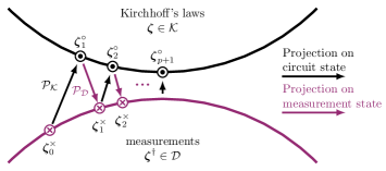
This minimization procedure is carried out until either $\bm{\zeta}^{\circ}_{p}$ and $\bm{\zeta}^{\times}_{p}$ do not change after two consecutive iterations or until a desired accuracy is reached. The accuracy at iteration $p$ can be measured in terms of the energy mismatch $\epsilon_{\mathrm{em},p}$, which is defined as

$$\epsilon_{\mathrm{em},p}^{2}=\left\|\bm{\zeta}^{\circ}_{p}-\bm{\zeta}^{\times}_{p}\right\|^{2}_{\tilde{G},\tilde{C},\tilde{L}},$$ (20)

which is essentially the weighted distance between the two states. Convergence is then achieved if the change in energy mismatch (20) between two consecutive iterations is below a user-defined tolerance. Once the data-driven solver has converged, we carry on with the next time step. The most recent data-driven solution is employed as starting point in the new time step.

It is customary that most of the elements in a circuit are well-known and model representations are available. In this case, various approaches combining exactly known models with data-driven computing have been proposed by the authors in [8]. We consider the least intrusive approach, where the minimization (16) is now performed to the known model representation. In addition, the weighting factors in (13) and (14) are chosen according to the known model coefficients. Furthermore, it has been shown by the authors that, for elements featuring a strongly nonlinear response and where only data-starved or unevenly filled measurement sets are available, constant weighting factors hinder the convergence rate of the data-driven solver [9]. Therefore, we follow the approach developed in [9] and choose the weighting factors to be the local tangent of the current state with respect to the surrounding states in the measurement set.

III Numerical Experiments

In the following, we consider different circuit configurations. To validate the data-driven solver, we generate artificial measurement data of increasing cardinality, for each of which the circuit is solved. At every time step $t_{k},\,k=1,\dots,K$, and at a specific element $X\in\{\mathrm{G},\mathrm{C},\mathrm{L}\}$, we calculate the energy mismatch with respect to an analytic reference solution, e.g., obtained with a traditional MNA solver utilizing the “true” circuit elements. The energy mismatch error is defined as

$$\epsilon_{\mathrm{EM},\tilde{X}}^{2}(t)=\left.\left\|(p_{\mathrm{ref}},q_{\mathrm{ref}})-(p,q)\right\|^{2}_{\tilde{X}}\right|_{t}.$$ (21)

Furthermore, we define the root mean square (RMS) error over the entire time interval as

$$\epsilon_{\mathrm{RMS},\tilde{X}} =\left(\frac{\int_{t_{0}}^{T}\epsilon_{\mathrm{EM},\tilde{X}}^{2}(t)\,\mathrm{d}t}{\int_{t_{0}}^{T}(\|(p_{\mathrm{ref}},q_{\mathrm{ref}})\|^{2}_{\tilde{X}}\,\mathrm{d}t}\right)^{\frac{1}{2}}$$ (22)

$$\approx\left(\frac{\sum_{k=0}^{K}\epsilon_{\mathrm{EM},\tilde{X}}^{2}(t_{k})}{\sum_{k=0}^{K}(\|(p_{\mathrm{ref}},q_{\mathrm{ref}})\|^{2}_{\tilde{X}})|_{t_{k}}}\right)^{\frac{1}{2}},$$

The weighting factors in (21) and (22) correspond to the actual model parameters which are used for the reference solution.

III-A Linear RC-circuit

For a first test, we consider an RC-circuit, with R and C in series. The circuit is excited by a constant voltage source. Furthermore, in order to use the analytical solution as a reference, we consider only linear elements. We employ a data-driven solver based on the backward Euler scheme and on the trapezoidal rule, where the resistor and the capacitor are assumed to be unknown and only measurement data is available for these elements. Additionally, solutions for different time step values, equivalently, numbers of time steps, are computed.

Figure 2: Linear RC-circuit: RMS error at the capacitor C over number of measurements. The horizontal lines mark the time-discretization errors for a traditional MNA circuit solver.

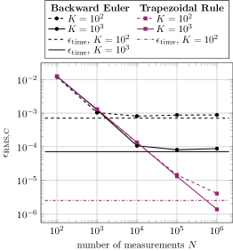
Figure 2 shows the RMS error for solutions obtained with the backward Euler method and the trapezoidal rule for different numbers of time steps. Furthermore, the RMS error for a traditional MNA solver is shown. The results show that the accuracy of the data-driven solution improves as more measurement data are employed. However, for certain combinations of employed measurement data and number of time steps, the convergence stagnates. To analyse this behavior, we consider the overall error of a state $(p,q)$ to the reference solution. The error is given as

$$\epsilon =\left\|(p_{\mathrm{ref}},q_{\mathrm{ref}})-(p,q)\right\|^{2}_{\tilde{X}}$$ (23)

$$=\left\|(p_{\mathrm{ref}}-p_{\mathrm{trad}},q_{\mathrm{ref}}-q_{\mathrm{trad}})-(p-p_{\mathrm{trad}},q-q_{\mathrm{trad}})\right\|^{2}_{\tilde{X}}$$

$$\leq\underbrace{\left\|(p_{\mathrm{ref}},q_{\mathrm{ref}})-(p_{\mathrm{trad}},q_{\mathrm{trad}})\right\|^{2}_{\tilde{X}}}_{\epsilon_{\mathrm{time}}}$$

$$+\underbrace{\left\|(p,q)-(p_{\mathrm{trad}},q_{\mathrm{trad}})\right\|^{2}_{\tilde{X}}}_{\epsilon_{\mathrm{data}}},$$

where $(p_{\mathrm{trad}},q_{\mathrm{trad}})$ is a state computed with a traditional MNA solver. Hence, the overall error can be decomposed into an error stemming from the time discretization scheme and an error attributed to the finite measurement data. This decomposition can be clearly observed in Figure 2. The figure shows several cases where extending the measurement set does not lead to an improvement in the accuracy. In those cases, the time-discretization error $\epsilon_{\mathrm{time}}$, is dominant and the accuracy of the data-driven solver stagnates at the accuracy level of the traditional solver. Hence, to avoid unnecessary computational costs, the time discretization scheme and the number of employed measurement data points should preferably be chosen according to one another. In cases where the time discretization error $\epsilon_{\mathrm{time}}$ is negligible, e.g., for $K=1000$ and the trapezoidal rule, the data-driven solver achieves a linear convergence rate with respect to the employed measurement data.

Figure 3: Linear RC-circuit: Voltage $v_{\mathrm{C}}$ at the capacitor over time. The plot shows the analytical reference solution, as well as data-driven solutions for an increasing number of measurement data.

Figure 4: Linear RC-circuit: Energy mismatch at the capacitor C over time. The error is shown for an increasing number of measurement data $N\in\left\{10^{2},10^{3},10^{4},10^{5},10^{6}\right\}$. The dashed line shows the voltage $v_{\mathrm{C}}$.

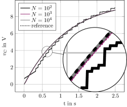
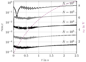
Next, we focus on the error attributed to the limited measurement data. Therefore, the circuit is simulated using the the trapezoidal rule and $K=1000$ time steps. The reference solution $v_{\mathrm{C}}$ as well as data-driven solutions for measurement data sets of increasing size are depicted in Figure 3. We can already qualitatively observe that, if the measurement data set is not sufficiently large, e.g., for $N=10^{2}$, the solution of the data-driven solver captures the behavior of the circuit, albeit a large error to the analytic solution remains. Furthermore, the figure shows that due to the discrete data, the solution is not continuous and exhibits jumps at certain time steps. More precisely, due to the finite data, the solver might select the same measurement state in consecutive time steps. However, as more data become available, these discontinuities are reduced. Figure 4 shows the energy mismatch to the reference solution over time for measurement sets of increasing cardinality. The figure clearly shows that the solution accuracy increases with the number of measurement data points.

III-B Nonlinear RC-circuit

We revisit the RC-circuit, yet this time we consider a voltage-dependent capacitor $C(v_{\mathrm{C}}(t))$. The response of the capacitor as well as the charge over the applied voltage is shown in Figure 5. This nonlinear response is the typical behavior of multi-layer ceramic capacitors, for which the capacitance drops rapidly for moderate voltages to a nearly constant value [25, 30].

Figure 5: Nonlinear RC-circuit: Voltage-dependent capacitor $C(v_{\mathrm{C}})$ and charge $q_{\mathrm{C}}(v_{\mathrm{C}})$ over applied voltage $v_{\mathrm{C}}$.

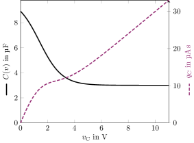
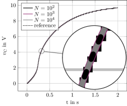
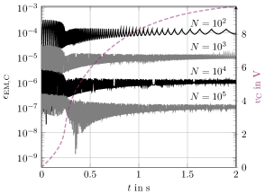
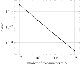
The data-driven solver treats the resistor as a known element. Contrarily, only measurement data is available for the voltage-dependent capacitor. To validate the results obtained with the data-driven solver, we generate measurement data sets of increasing cardinality. Both the reference solver and the data-driven solver employ the trapezoidal rule for time discretization. Figure 6 shows the capacitor voltage over time. Similar to the linear case, the data-driven solution shows large jumps between the time steps if the number of measurement data points is not sufficiently large. As the number of measurements increases, the data-driven solution becomes increasingly smoother and eventually identical to the conventional MNA solution. This is also evident by the results shown in Figure 8 regarding the RMS error over time for an increasing number of measurement data points. Similar to the linear RC circuit, a linear convergence rate with respect to the number of measurement points is observed. The energy mismatch over time and for measurement sets of increasing cardinality is shown in Figure 7. Again, the figure clearly shows that the solution accuracy increases with the number of measurement data points. We also observe that the error in time is slightly larger in the strongly nonlinear region, that is, for $t<$0.5\text{\,}\mathrm{s}$$, respectively for $v_{\mathrm{C}}<$4\text{\,}\mathrm{V}$$.

Figure 6: Nonlinear RC-circuit: voltage $v_{\mathrm{C}}$ at the capacitor over time. The plot shows the analytical reference solution, as well as data-driven solutions for a increasing number of measurement data $N\in\left\{10^{2},10^{3},10^{4}\right\}$.

Figure 7: Nonlinear RC-circuit: Energy mismatch at the capacitor C over time. The error is shown for an increasing number of measurement data $N\in\left\{10^{2},10^{3},10^{4},10^{5}\right\}$. The dashed line shows the voltage $v_{\mathrm{C}}$.

Figure 8: Nonlinear RC-circuit: RMS error at the capacitor C over number of measurements.

III-C Half-wave rectifier

Figure 9: Half-wave rectifier circuit.

The next test case considers the well-known half-wave rectifier circuit, depicted in Figure 9. The circuit elements are $R_{\mathrm{C}}=$1\text{\,}\mathrm{k\SIUnitSymbolOhm}$$, $R_{\mathrm{D}}=$10\text{\,}\mathrm{m\SIUnitSymbolOhm}$$, $C=$100\text{\,}\mathrm{\SIUnitSymbolMicro F}$$ and $v_{\mathrm{src}}=$5\text{\,}\mathrm{V}$\sin(\omega t)$, where $\omega=2\pi f$ and $f=$100\text{\,}\mathrm{Hz}$$. The diode is modeled using the Shockley diode model [26], such that

$$i(t)=i_{\mathrm{s}}\left(\mathrm{e}^{\frac{v_{\mathrm{D}}(t)}{nv_{\mathrm{T}}}}-1\right),$$ (24)

where $v_{\mathrm{D}}$ is the voltage at the diode, $i_{\mathrm{s}}=$2.52\text{\,}\mathrm{nA}$$ is the saturation current, $v_{\mathrm{T}}=$25.85\text{\,}\mathrm{mV}$$ is the thermal voltage, here for $T=$300\text{\,}\mathrm{K}$$, and $n=1.752$ is the ideality factor.

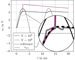
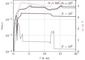
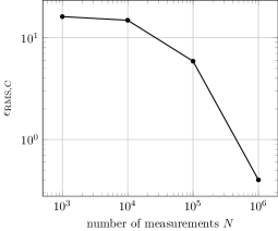
We assume that the resistors and the capacitor are known elements, whereas the diode is only known by measurement data. The parasitic resistor $R_{\mathrm{D}}$ is part of the circuit model in the ngspice simulation [24]. Hence, the measurement data is generated from the diode model including the parasitic resistor $R_{\mathrm{D}}$. The data-driven solutions are compared to a reference solution obtained with ngspice. For both the reference and the data-driven solutions, $K=400$ time steps are used. The data-driven solver is based on the trapezoidal rule. Figure 10 shows the output voltage $v_{\mathrm{C}}$ of the half-wave rectifier. The figure clearly shows that the data-driven solution becomes more accurate if more measurement data is employed. However, we also observe that a rather large number of measurement data is needed to achieve an adequately accurate solution. This behavior can also be seen in Figure 11, which shows the energy mismatch over time, as well as in Figure 12, which shows the RMS error at the capacitor. The reduced convergence rate can be explained by the switching behavior of the diode. That is, the distance-minimizing data-driven solver faces problems in the regime where the current of the diode remains almost constant, i.e., for $v_{\mathrm{D}}\ll v_{\mathrm{fv}}$, where $v_{\mathrm{fv}}$ is the forward threshold voltage.

Figure 10: Half-wave rectifier: Voltage $v_{\mathrm{C}}$ at the capacitor over time. The plot shows the reference solution obtained with ngspice and data-driven solutions for an increasing number of measurement data $N\in\left\{10^{5},10^{6}\right\}$.

Figure 11: Half-wave rectifier: Energy mismatch at the capacitor C over time. The error is shown for an increasing number of measurement data $N\in\left\{10^{3},10^{4},10^{5},10^{6}\right\}$. The dashed line shows the output voltage $v_{\mathrm{C}}$.

Figure 12: Half-wave rectifier: RMS error at the capacitor C over number of measurements.

IV Computational cost

In the following, we briefly discuss the computational cost of the data-driven MNA solver. For a more detailed discussion on the computational complexity of data-driven solvers, the reader is referred to [9, 10].

In each data-driven iteration, we have to solve a linear system of size $2n-2+n_{\mathrm{G}}+n_{\mathrm{C}}+3n_{\mathrm{L}}+2n_{\mathrm{V}}$. The number of data-driven iterations is strongly connected to the number of employed measurement data. Furthermore, strongly nonlinear element responses also demand for more data-driven iterations. In the case of the linear RC-circuit, the number of data-driven iterations per time step vary from $5$ (for $N=10^{2}$) to $45$ (for $N=10^{6}$). For the nonlinear RC-circuit, the number of iterations depends on the current operation point in the $(u_{\mathrm{C}},q_{\mathrm{C}})$ phase-space. In the region where the relation is almost linear, the number of data-driven iterations is similar to the ones of the linear RC-circuit. If the operation point is in the strongly nonlinear regions, the iterations range from $20$ (for $N=10^{2}$) to $140$ (for $N=10^{6}$). In comparison, the traditional solver must solve the nonlinear problem at each time step, which resulted in $12$ iterations on average in the case of the nonlinear RC circuit.

Hence, the data-driven MNA solver in its current implementation still needs up to ten times more simulation time. This is the price to pay for the benefit of not requiring models for the circuit elements. It is expected that progress in data-processing will further decrease the gap between traditional and data-driven MNA solvers.

Last, we note that the aforementioned remarks on the computational cost of the traditional and the data-driven MNA solvers only take into account the aspect of computational complexity in terms of linear system size, system solutions, and solver iterations. That is, this discussion does not include the effort that is usually needed to identify and construct model representations to be used within traditional MNA solvers. While this element modeling effort is difficult to assess, it must be underlined that the modeling step is bypassed altogether when the data-driven solver is employed.

V Conclusion

This paper proposes a data-driven MNA circuit solver, which relies on Kirchhoff’s laws and on measurement data for the elements instead of traditional element models. The solver was first applied to a linear RC-circuit, where an investigation on the different approximation errors concluded that the available measurement data and the time step employed in the time integration method should match one another in order to avoid unnecessary computational costs. The solver was additionally applied to a nonlinear RC-circuit with a voltage-dependent capacitor and to a half-wave rectifier with a data-driven diode. In the former case, the solver achieves a linear convergence rate with respect to the number of measurement data points. This convergence rate is not observed in the latter case, where the switching behavior of the diode model, in particular the regime before the threshold voltage, hinders solver convergence and demands for comparatively large data sets.

The numerical results have shown that the data-driven MNA solver developed in this work constitutes a viable alternative for standard MNA circuit simulation, in particular for cases featuring elements with an unknown model representation, but for which measurement data are available instead. Due to the identified limitations of the data-drive MNA solver in handling circuits with a switching behavior, such as the half-wave rectifier unit shown in Section III-C, future research efforts shall concentrate on a more in-depth investigation of these specific cases. Additional topics for future research include data-driven circuit simulation incorporating noisy measurement data, as well as the handling of elements that cannot be described through the classical two-port network model.

References

- [1] K. Aadithya et al. “Data-driven Compact Models for Circuit Design and Analysis” In Proceedings of The First Mathematical and Scientific Machine Learning Conference 107, Proceedings of Machine Learning Research PMLR, 2020, pp. 555–569
- [2] Miona V Andrejević and Vančo B Litovski “Electronic circuits modeling using artificial neural networks” In Journal of Automatic Control 13.1, 2003, pp. 31–37
- [3] Xiaowei Bai et al. “A data-driven approach for instability analysis of thin composite structures” In Computers & Structures 273, 2022 DOI: https://doi.org/10.1016/j.compstruc.2022.106898
- [4] P. Carrara, L. De Lorenzis, L. Stainier and M. Ortiz “Data-driven fracture mechanics” In Computer Methods in Applied Mechanics and Engineering 372, 2020, pp. 113390 DOI: https://doi.org/10.1016/j.cma.2020.113390
- [5] Xi Chen et al. “Application of neural networks for integrated circuit modeling” In Advances in Neural Networks-ISNN 2006: Third International Symposium on Neural Networks, Chengdu, China, May 28-June 1, 2006, Proceedings, Part III 3, 2006, pp. 1304–1312 Springer
- [6] Zaichen Chen, Maxim Raginsky and Elyse Rosenbaum “Verilog-A compatible recurrent neural network model for transient circuit simulation” In 2017 IEEE 26th Conference on Electrical Performance of Electronic Packaging and Systems (EPEPS), 2017, pp. 1–3 IEEE
- [7] Tomislav Ćirić et al. “Neural based lumped element model of capacitive RF MEMS switches” In Frequenz 72.11-12 De Gruyter, 2018, pp. 539–546
- [8] H. De Gersem et al. “Magnetic Field Simulation with Data-Driven Material Modeling” In IEEE Transactions on Magnetics 56.8, 2020, pp. 1–6 DOI: 10.1109/TMAG.2020.3002092
- [9] Armin Galetzka, Dimitrios Loukrezis and Herbert De Gersem “Data-driven solvers for strongly nonlinear material response” In International Journal for Numerical Methods in Engineering 122.6, 2021, pp. 1538–1562 DOI: https://doi.org/10.1002/nme.6589
- [10] Armin Galetzka, Dimitrios Loukrezis and Herbert De Gersem “Three-dimensional data-driven magnetostatic field computation using real-world measurement data” In COMPEL - The international journal for computation and mathematics in electrical and electronic engineering, 2021 DOI: https://doi.org/10.1108/COMPEL-06-2021-0219
- [11] Paul-William Gerbaud, David Néron and Pierre Ladevèze “Data-driven elasto-(visco)-plasticity involving hidden state variables” In Computer Methods in Applied Mechanics and Engineering 402, 2022, pp. 115394 DOI: https://doi.org/10.1016/j.cma.2022.115394
- [12] Dirk Gorissen, Luciano De Tommasi, Karel Crombecq and Tom Dhaene “Sequential modeling of a low noise amplifier with neural networks and active learning” In Neural Computing and Applications 18 Springer, 2009, pp. 485–494
- [13] Hanene Ben Hammouda, Mongia Mhiri, Zièd Gafsi and Kamel Besbes “Neural-based models of semiconductor devices for SPICE simulator” In American Journal of Applied Sciences 5.4, 2008, pp. 385–391
- [14] Chung-Wen Ho, A. Ruehli and P. Brennan “The modified nodal approach to network analysis” In IEEE Transactions on Circuits and Systems 22.6, 1975, pp. 504–509 DOI: 10.1109/TCS.1975.1084079
- [15] Humayun Kabir et al. “Smart Modeling of Microwave Devices” In IEEE Microwave Magazine 11.3, 2010, pp. 105–118 DOI: 10.1109/MMM.2010.936079
- [16] T. Kirchdoerfer and M. Ortiz “Data-driven computational mechanics” In Computer Methods in Applied Mechanics and Engineering 304, 2016, pp. 81 –101 DOI: https://doi.org/10.1016/j.cma.2016.02.001
- [17] T. Kirchdoerfer and M. Ortiz “Data Driven Computing with noisy material data sets” In Computer Methods in Applied Mechanics and Engineering 326, 2017, pp. 622 –641 DOI: https://doi.org/10.1016/j.cma.2017.07.039
- [18] Trenton Kirchdoerfer and Michael Ortiz “Data-driven computing in dynamics” In International Journal for Numerical Methods in Engineering 113.11 Wiley Online Library, 2018, pp. 1697–1710
- [19] Dominik K. Klein, Rogelio Ortigosa, Jesús Martínez-Frutos and Oliver Weeger “Finite electro-elasticity with physics-augmented neural networks” In Computer Methods in Applied Mechanics and Engineering 400, 2022, pp. 115501 DOI: https://doi.org/10.1016/j.cma.2022.115501
- [20] Nikhil M. Kriplani, Stephen Bowyer, Jennifer Huckaby and Michael B. Steer “Modelling of an Esaki Tunnel Diode in a Circuit Simulator” In Active and Passive Electronic Components 2011 Hindawi Publishing Corporation, 2011 DOI: 10.1155/2011/830182
- [21] Stefan Kurz et al. “Hybrid modeling: towards the next level of scientific computing in engineering” In Journal of Mathematics in Industry 12.1, 2022, pp. 8 DOI: 10.1186/s13362-022-00123-0
- [22] Mingda Li, Ozan İrsoy, Claire Cardie and Huili Grace Xing “Physics-inspired neural networks for efficient device compact modeling” In IEEE Journal on Exploratory Solid-State Computational Devices and Circuits 2 IEEE, 2016, pp. 44–49
- [23] Vančo B Litovski, Željko Mrčarica and Tihomir Ilić “Simulation of non-linear magnetic circuits modelled using artificial neural network” In Simulation Practice and Theory 5.6 Elsevier, 1997, pp. 553–570
- [24] Paolo Nenzi and Holger Vogt “Ngspice Users Manual Version 23” June, 2011
- [25] Stanislav Scheier and Stephan Frei “Characterization and modeling of ESD-behavior of multi layer ceramic capacitors” In 2013 International Symposium on Electromagnetic Compatibility, 2013, pp. 1028–1033
- [26] W. Shockley “The theory of p-n junctions in semiconductors and p-n junction transistors” In The Bell System Technical Journal 28.3, 1949, pp. 435–489 DOI: 10.1002/j.1538-7305.1949.tb03645.x
- [27] Kashvi Taunk, Sanjukta De, Srishti Verma and Aleena Swetapadma “A brief review of nearest neighbor algorithm for learning and classification” In 2019 International Conference on Intelligent Computing and Control Systems (ICCS), 2019, pp. 1255–1260 IEEE
- [28] Ernst Wit, Edwin van den Heuvel and Jan-Willem Romeijn “‘All models are wrong…’: an introduction to model uncertainty” In Statistica Neerlandica 66.3 Wiley Online Library, 2012, pp. 217–236
- [29] A Hafid Zaabab, Qi-Jun Zhang and Michel Nakhla “A neural network modeling approach to circuit optimization and statistical design” In IEEE Transactions on Microwave Theory and Techniques 43.6 IEEE, 1995, pp. 1349–1358
- [30] Ilya Zeltser and Shmuel Ben-Yaakov “On SPICE Simulation of Voltage-Dependent Capacitors” In IEEE Transactions on Power Electronics 33.5, 2018, pp. 3703–3710 DOI: 10.1109/TPEL.2017.2766025